Embed Size (px)
Citation preview
Biosignal filtering and artifact rejection, Part II
Biosignal processing, 521273SAutumn 2017
Example: eye blinks interfere with EEG
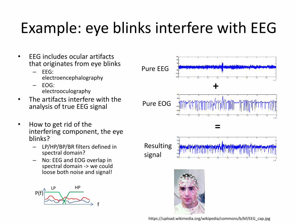
• EEG includes ocular artifacts that originates from eye blinks– EEG:
electroencephalography– EOG:
electrooculography
• The artifacts interfere with the analysis of true EEG signal
• How to get rid of the interfering component, the eye blinks?– LP/HP/BP/BR filters defined in
spectral domain?– No: EEG and EOG overlap in
spectral domain -> we could loose both noise and signal!
Pure EEG
Pure EOG
Resultingsignal
+
=
f
P(f)LP HP
https://upload.wikimedia.org/wikipedia/commons/b/bf/EEG_cap.jpg
Example: eye blinks interfere with EEG
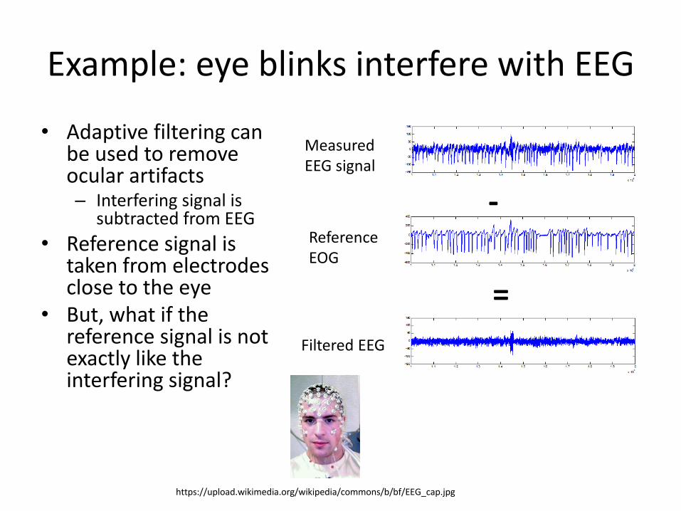
• Adaptive filtering can be used to remove ocular artifacts– Interfering signal is
subtracted from EEG
• Reference signal is taken from electrodes close to the eye
• But, what if the reference signal is not exactly like the interfering signal?
Filtered EEG
ReferenceEOG
MeasuredEEG signal
-
=
https://upload.wikimedia.org/wikipedia/commons/b/bf/EEG_cap.jpg
LMS adaptive filtering (Least Mean Square)
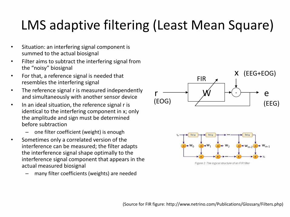
• Situation: an interfering signal component is summed to the actual biosignal
• Filter aims to subtract the interfering signal from the “noisy” biosignal
• For that, a reference signal is needed that resembles the interfering signal
• The reference signal r is measured independently and simultaneously with another sensor device
• In an ideal situation, the reference signal r is identical to the interfering component in x; only the amplitude and sign must be determined before subtraction– one filter coefficient (weight) is enough
• Sometimes only a correlated version of the interference can be measured; the filter adapts the interference signal shape optimally to the interference signal component that appears in the actual measured biosignal– many filter coefficients (weights) are needed
-Wr e
x (EEG+EOG)
(EEG)(EOG)
FIR
(Source for FIR figure: http://www.netrino.com/Publications/Glossary/Filters.php)
w0 w1 w2 wm-1wm-2
LMS adaptive filtering (Least Mean Square)
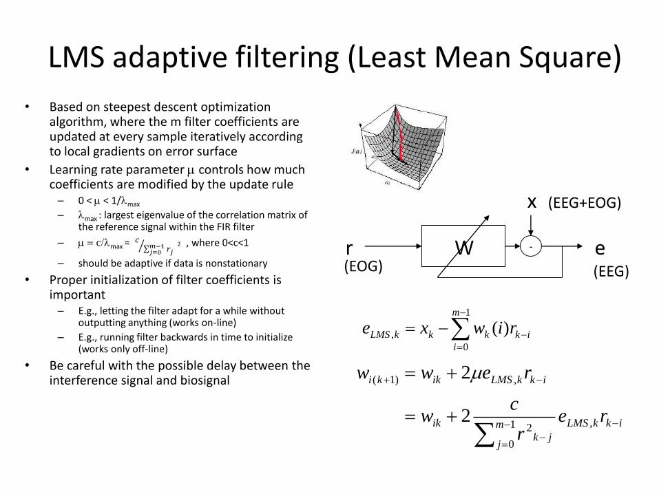
• Based on steepest descent optimization algorithm, where the m filter coefficients are updated at every sample iteratively according to local gradients on error surface
• Learning rate parameter m controls how much coefficients are modified by the update rule – 0 < m < 1/lmax
– lmax : largest eigenvalue of the correlation matrix of the reference signal within the FIR filter
– m = c/lmax = 𝑐 𝑗=0𝑚−1 𝑟𝑗
2 , where 0<c<1
– should be adaptive if data is nonstationary
• Proper initialization of filter coefficients is important– E.g., letting the filter adapt for a while without
outputting anything (works on-line)
– E.g., running filter backwards in time to initialize (works only off-line)
• Be careful with the possible delay between the interference signal and biosignal
=
=1
0
, )(m
i
ikkkkLMS riwxe
ikkLMSm
jjk
ik
ikkLMSikki
rer
cw
reww
=
=
=
,1
0
2
,)1(
2
2m
-Wr e
x (EEG+EOG)
(EEG)(EOG)
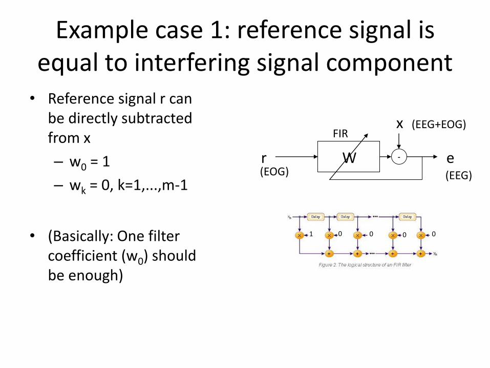
Example case 1: reference signal is equal to interfering signal component• Reference signal r can
be directly subtracted from x
– w0 = 1
– wk = 0, k=1,...,m-1
• (Basically: One filter coefficient (w0) should be enough)
-Wr e
x (EEG+EOG)
(EEG)(EOG)
FIR
1 0 0 00
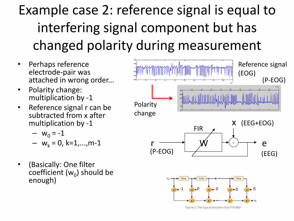
Example case 2: reference signal is equal to interfering signal component but has
changed polarity during measurement• Perhaps reference
electrode-pair was attached in wrong order...
• Polarity change: multiplication by -1
• Reference signal r can be subtracted from x after multiplication by -1– w0 = -1– wk = 0, k=1,...,m-1
• (Basically: One filter coefficient (w0) should be enough)
-Wr e
x (EEG+EOG)
(EEG)(P-EOG)
FIR
-1 0 0 00
Reference signal(EOG)
Polaritychange
(P-EOG)
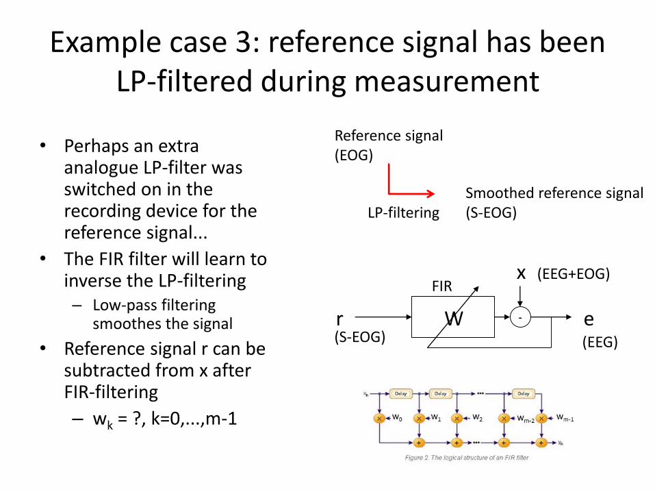
Example case 3: reference signal has been LP-filtered during measurement
• Perhaps an extra analogue LP-filter was switched on in the recording device for the reference signal...
• The FIR filter will learn to inverse the LP-filtering– Low-pass filtering
smoothes the signal
• Reference signal r can be subtracted from x after FIR-filtering
– wk = ?, k=0,...,m-1
-Wr e
x (EEG+EOG)
(EEG)(S-EOG)
FIR
Reference signal(EOG)
Smoothed reference signal(S-EOG)LP-filtering
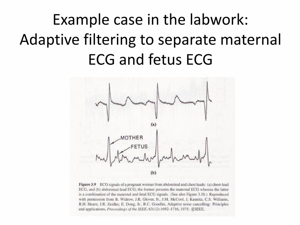
Example case in the labwork:Adaptive filtering to separate maternal
ECG and fetus ECG
Selected references
Course text book: Section 3.6 (2002) / Section 3.9 (2015), Adaptive filters for removal of interference
Case study: Removing respiration component from heart rate signal using LMS adaptive filtering
Source: Tiinanen S, Tulppo MP, Seppänen T. Reducing the Effect of Respiration in Baroreflex Sensitivity Estimation with Adaptive Filtering. IEEE Transactions on Biomedical Engineering 2008;55(1):51-59.
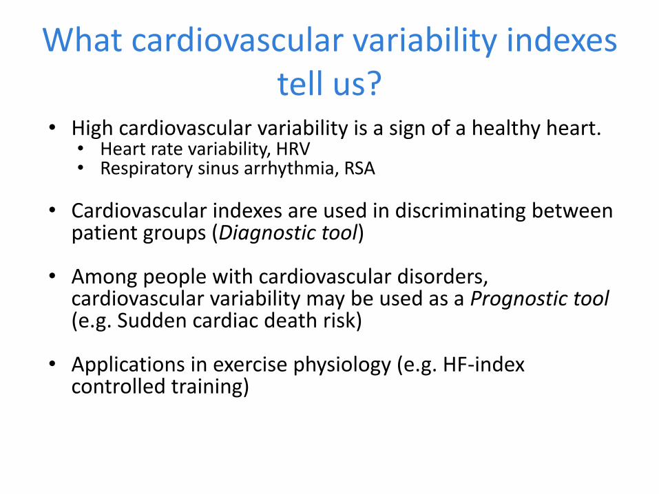
What cardiovascular variability indexes tell us?
• High cardiovascular variability is a sign of a healthy heart.• Heart rate variability, HRV• Respiratory sinus arrhythmia, RSA
• Cardiovascular indexes are used in discriminating between patient groups (Diagnostic tool)
• Among people with cardiovascular disorders, cardiovascular variability may be used as a Prognostic tool (e.g. Sudden cardiac death risk)
• Applications in exercise physiology (e.g. HF-index controlled training)
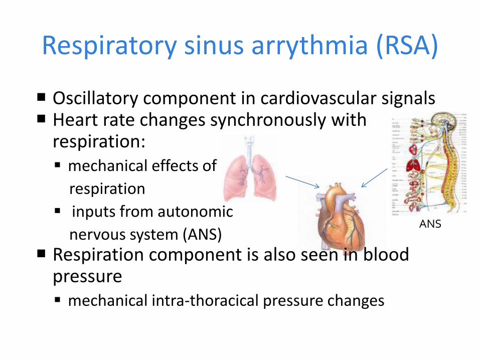
Respiratory sinus arrythmia (RSA)
Oscillatory component in cardiovascular signals Heart rate changes synchronously with
respiration: mechanical effects of
respiration
inputs from autonomic
nervous system (ANS) Respiration component is also seen in blood
pressure mechanical intra-thoracical pressure changes
ANS
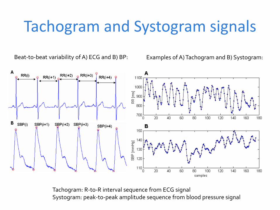
Tachogram and Systogram signals
Beat-to-beat variability of A) ECG and B) BP: Examples of A) Tachogram and B) Systogram:
Tachogram: R-to-R interval sequence from ECG signalSystogram: peak-to-peak amplitude sequence from blood pressure signal
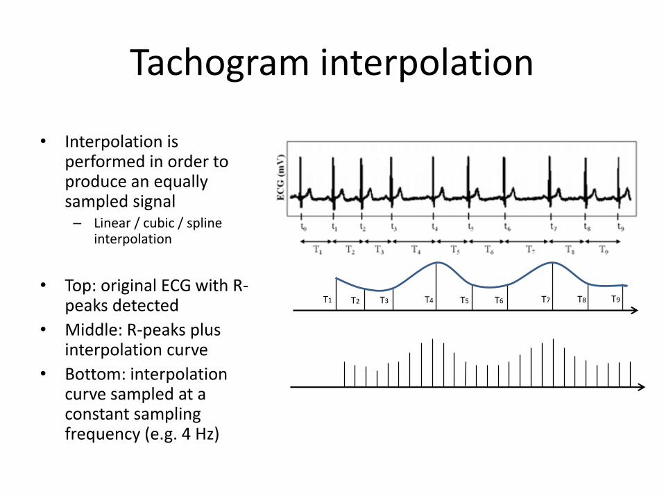
Tachogram interpolation
• Interpolation is performed in order to produce an equally sampled signal– Linear / cubic / spline
interpolation
• Top: original ECG with R-peaks detected
• Middle: R-peaks plus interpolation curve
• Bottom: interpolation curve sampled at a constant sampling frequency (e.g. 4 Hz)
T1 T2 T3 T4 T5 T6 T7 T8 T9
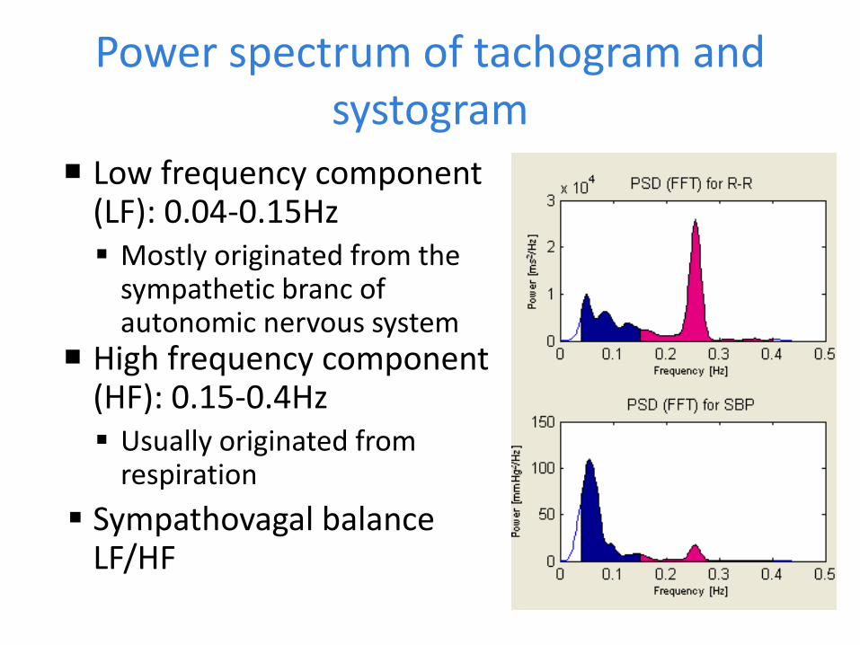
Power spectrum of tachogram and systogram
Low frequency component (LF): 0.04-0.15Hz Mostly originated from the
sympathetic branc of autonomic nervous system
High frequency component (HF): 0.15-0.4Hz Usually originated from
respiration
Sympathovagal balance LF/HF
Motivation
Why RSA extraction?• If respiration rate is low, RSA overlaps the low
frequency (LF) range - > Biased cardiovascular indices!
• The extracted RSA component itself is also a useful index of cardiovascular system.
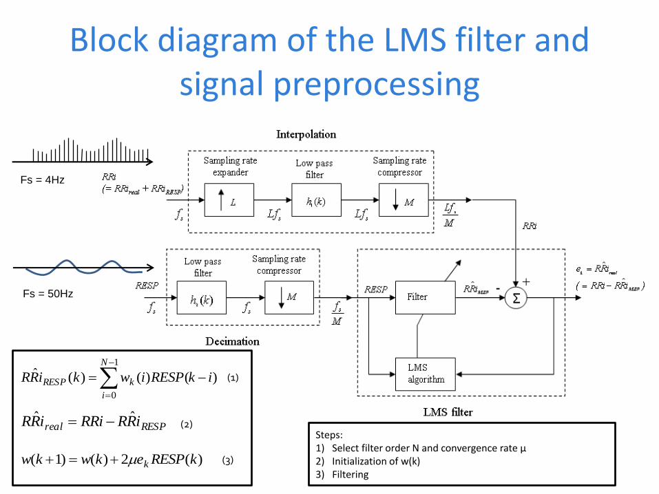
Block diagram of the LMS filter and signal preprocessing
)()()(ˆ1
0
ikRESPiwkiRR
N
i
kRESP =
=
RESPreal iRRRRiiRR ˆˆ =
)(2)()1( kRESPekwkw km=
(1)
(2)
(3)
Steps:1) Select filter order N and convergence rate µ2) Initialization of w(k)3) Filtering
Fs = 4Hz
Fs = 50Hz
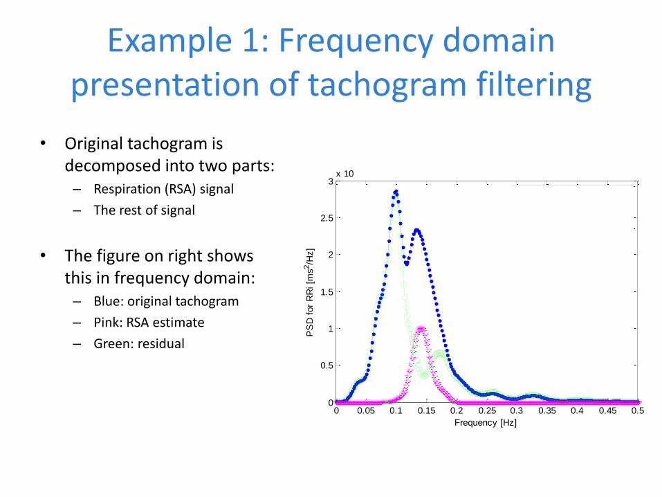
Example 1: Frequency domain presentation of tachogram filtering
• Original tachogram is decomposed into two parts:– Respiration (RSA) signal
– The rest of signal
• The figure on right shows this in frequency domain:– Blue: original tachogram
– Pink: RSA estimate
– Green: residual
0 0.05 0.1 0.15 0.2 0.25 0.3 0.35 0.4 0.45 0.50
0.5
1
1.5
2
2.5
3x 10
4
Frequency [Hz]
PS
D f
or
RR
i [m
s2/H
z]
RRi(blue)
RRi estimate(green)
RSA estimate(pink)
0 0.05 0.1 0.15 0.2 0.25 0.3 0.35 0.4 0.45 0.50
0.5
1
1.5
2
2.5
3x 10
4
Frequency [Hz]
PS
D f
or
RR
i [m
s2/H
z]
RRi(blue)
RRi estimate(green)
RSA estimate(pink)
0 0.05 0.1 0.15 0.2 0.25 0.3 0.35 0.4 0.45 0.50
20
40
60
80
100
120
140
Frequency [Hz]
PS
D f
or
SB
P [
mm
Hg
2/H
z]
SBP(blue)
SBP estimate(green)
RSA estimate(pink)
0 0.05 0.1 0.15 0.2 0.25 0.3 0.35 0.4 0.45 0.50
20
40
60
80
100
120
140
Frequency [Hz]
PS
D f
or
SB
P [
mm
Hg
2/H
z]
SBP(blue)
SBP estimate(green)
RSA estimate(pink)
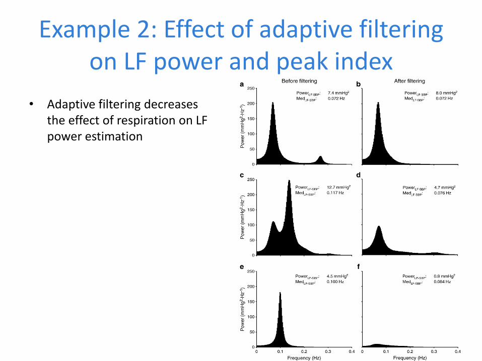
Example 2: Effect of adaptive filtering on LF power and peak index
• Adaptive filtering decreases the effect of respiration on LF power estimation
Summary of the case study
• LF powers and their derivative indexes (HRV) are less biased if respiratory component is removed from LF range.
• LF peak index (the frequency at maximum power) is distorded by low respiration rate-> Adaptive filtering corrects the distortion