Biorthogonal partners and applications - Signal Processing ... · Biorthogonal Partners and Applications P. P. Vaidyanathan, Fellow, IEEE, and Bojan Vrcelj, Student Member, IEEE Abstract—

IEEE TRANSACTIONS ON SIGNAL PROCESSING, VOL. 49, NO. 5, MAY 2001 1013

Biorthogonal Partners and ApplicationsP. P. Vaidyanathan, Fellow, IEEE,and Bojan Vrcelj, Student Member, IEEE

Abstract—Two digital filters ( ) and ( ) are said to bebiorthogonal partners of each other if their cascade ( ) ( )satisfies the Nyquist or zero-crossing property. Biorthogonal part-ners arise in many different contexts such as filterbank theory,exact and least squares digital interpolation, and multiresolutiontheory. They also play a central role in the theory of equaliza-tion, especially, fractionally spaced equalizers in digital commu-nications. In this paper, we first develop several theoretical prop-erties of biorthogonal partners. We also develop conditions for theexistence of biorthogonal partners and FIR biorthogonal pairs andestablish the connections to the Riesz basis property. We then ex-plain how these results play a role in many of the above-mentionedapplications.

I. INTRODUCTION

T WO DIGITAL filters and are said to bebiorthogonal partners of each other if their cascade

satisfies the Nyquist or zero-crossing property.Biorthogonal partners1 arise in many different contexts such asfilterbank theory [1], [23], [27], exact and least-squares digitalinterpolation [20], sampling theory [22], and multiresolutiontheory [10]. They also play a central role in the theory ofequalization, especially fractionally spaced equalizers in digitalcommunications [17]. In this paper, we first develop severaltheoretical properties of biorthogonal partners. We then explainthe above-mentioned applications that use this concept directlyor indirectly.

A. Outline and Relation to Past Work

The paper contains several new results and new proofs ofwell-known results. One main contribution here is to glue to-gether certain widely known ideas in a unified manner underone cover. In Section II, we introduce the precise definition ofbiorthogonal partners. We derive a general closed-form expres-sion for a filter to be a biorthogonal partner of . Wealso develop a set of necessary and sufficient conditions on anFIR or IIR transfer function such that there exists an FIRbiorthogonal partner . This section also provides a deeperdiscussion on the existence of biorthogonal partners. In Sec-tion III, we study the application of these ideas in digital interpo-lation. This application also reveals the conditions on thatallow the existence of a biorthogonal partner. It also places in

Manuscript received April 21, 2000; revised January 29, 2001. Thiswork was supported in part by the Office of Naval Research under GrantN00014-99-1-1002 and by Microsoft Research, Redmond, WA. The associateeditor coordinating the review of this paper and approving it for publicationwas Prof. Hideaki Sakai.

The authors are with the Department of Electrical Engineering, CaliforniaInstitute of Technology, Pasadena, CA 91125 USA (e-mail: [email protected]).

Publisher Item Identifier S 1053-587X(01)03347-5.

1The term “biorthogonal partner” has not been used in the past. We use it herebecause of the frequent need for a descriptive term.

evidence the connection to linear independence and Riesz basisproperty of the shifted impulse responses of .This work is closely related to the concept of oblique projectionsstudied extensively by Aldroubiet al.and Cohenet al. [2]–[5].

Section V reviews the role of biorthogonal partners in theleast squares approximation of signals using interpolationmodels. Although this idea originated in the context of splineinterpolation [7], its efficient implementation became pos-sible because of the work by Unseret al. [20], [21], whodeveloped fundamental digital filter structures for efficientimplementation of the same. Applications of biorthogonalpartners in the interpolation of signals based on continuoustime models (e.g., spline models [13], [19]) is also discussed inSection VI. We also show that an all-FIR spline interpolation issometimes possible, unlike the more well-known methods ofUnseret al., which use an IIR/FIR combination [19]. The roleof biorthogonal partners in multiresolution theory is describedin Section VI-C. We show in particular that an FIR methodfor the computation of multiresolution coefficients is possible,without resorting to the traditional high degree of oversampling.Finally, in Section VII, we review applications in the theory offractionally spaced equalizers for digital communications [12],[17].

B. Notations

Unless mentioned otherwise, all notations are as in [23]. Weuse the notations and to denote the deci-mated version and its -transform. The expanded ver-sion

mul of

otherwise

is similary denoted by , and its -transform isdenoted by . Notice that

so that

The tilde notation is defined by so thaton the unit circle, . Thus, evaluatedon the unit circle is the magnitude square function. In situationswhere the -transform does not exist in the conventional sense(e.g., ideal filters), the notationstands for so that isthe frequency response .

II. BIORTHOGONAL PARTNERS: DEFINITION AND PROPERTIES

Two transfer functions and are said to form abiorthogonal pairwith respect to an integer if

(1)

1053–587X/01$10.00 © 2001 IEEE

1014 IEEE TRANSACTIONS ON SIGNAL PROCESSING, VOL. 49, NO. 5, MAY 2001

Fig. 1. Nyquist(M ) property ofP (z) demonstrated forM = 3.

(a)

(b)

Fig. 2. Interpretation of biorthogonal partnersH(z); F (z) in terms of signalflowgraphs.

We say that is abiorthogonal partner(or just partner) of. Notice that if is changed, the two filters may not re-

main partners. The term “with respect to” is usually under-stood from the context and is never mentioned unless there isa possible confusion. Evidently, and can be inter-changed without altering this property. Equation (1) is equiv-alent to the statement that the impulse response of theproduct filter satisfies theNyquist(M)con-dition

That is, the -fold decimation of yields the impulse(Fig. 1). We can regard and as any pair that definesa factorizationof a Nyquist( ) filter .

Notice that every pair of filters in an-channel perfect reconstruction (PR or biorthogonal) filter-

bank satisfies this condition. This is also the reason for thephrase “biorthogonal pair.” Recall that the “multirate” systemshown in Fig. 2(a) is just an LTI (single rate) system withtransfer function (see “polyphase identity”[23]). Thus, the implication of (1) is that the system shown inFig. 2(a) is an identity system. That is, the decimation filter[ followed by ] is diagrammatically the right inverseof the interpolation filter [ followed by ] [Fig. 2(b)].

Given a transfer function and the integer , does abiorthogonal partner always exist? When is it unique? If

is FIR, then under what conditions does there exist an FIRbiorthogonal partner ? For rational , can we get FIRpartners? In this section, we answer these questions.

A. General Expression

We first derive a general expression for interms of . In the following theorem, note that thenotation stands for , where

.

(a)

(b)

Fig. 3. Pertaining to the proof of Theorem 1.

Theorem 1—General Form of Biorthogonal Partner:Thetransfer function satisfies if and onlyif it can be expressed in the form

(2)

for some transfer function .Proof: Given a transfer function of the above form,

we have

which proves the “if part.” Conversely, suppose is suchthat . Consider the interpolation schemeshown in Fig. 3(a), where is an arbitrary input andthe output of . If we cascade and the decimator

as shown in the figure, then the output is because. The important point is that this also means

that the signal input to the system of Fig. 3(b) comes outas . This is because by definition is the output of theleft half in Fig. 3(a) driven by . Thus

which indeed can be rewritten as (2).Notice in the proof that since is arbi-

trary, it can be chosen so that the denominator of (2) is nonzerofor all . In general, a biorthogonal partner may or maynot exist, and when it exists, it may not be unique. It followsfrom Theorem 1 that a stable biorthogonal partner can be foundif and only if there exists a such that isnonzero for all . We will return to a more insightful discussionof existence issues in Section IV. Here are some special situa-tions of interest.

1) If for all , then istheoretically stable (though not necessarily causal). Thisis conceptually the simplest biorthogonal partner.

2) If hasunit circle zeros, then is nota stable filter. However, we can often get other solutions.For example, suppose the decimated version [23]

VAIDYANATHAN AND VRCELJ: BIORTHOGONAL PARTNERS AND APPLICATIONS 1015

(a)

(b)

(c)

(d)

Fig. 4. Block diagram interpretation of the proof of Theorem 2. (a) Cascade of interpolator and decimator. (b) Redrawing in polyphase form. (c) Basic multirateidentity. (d) Simplification of part (b) using the identity.

is nonzero for all . Then, we can set in (2) toobtain the stable biorthogonal partner

3) The preceding examples show that the biorthogonalpartner in general isnot unique. To get yet anothersolution, consider the filter

Since , we haveso that on the unit circle. Thepreceding solution is a special case of (2) with

and works as long as is nonzerofor all . This is a “popular solution” in some sense andis described in greater detail in Section V in the contextof least squares approximations.

4) If and are biorthogonal partners of ,then so is the convex combination

.5) Suppose is nonzero only in a set of measure

in [e.g., ideal lowpass with totalpassband width ]. Then, has thesame property so that

cannot fill the region completely. Theredoesnot exista biorthogonal partner for this .

6) If we replace with in (2), then thepart merely cancels and leaves unchanged. There-fore, is not unique for a given pair. If

and are two possible choices, then we canverify that for some [to seethis, just divide one representation of by the other].

B. Rational and FIR Cases

In practice the situation of most interest is the case whereis rational, that is, where andare polynomials in . In this case the trivial choice

gives a rational biorthogonal partner. Thisis stable (though possibly noncausal) as long as has nounit circle zeros. If is FIR, then the trivial choice

yields an allpole IIR filter. A question of significantinterest is this: if is FIR, can we obtain an FIR solution

? The answer is provided below. This is key to some of theapplications described in the next several sections. In fact, thistheorem is applicable in nearly the same form in the theory offractionally spaced equalizers [15]–[17].

Theorem 2—Existence of FIR Partner:Supposeis FIR. Express it in the polyphase form

. Then, there exists an FIR filtersuch that if and only if the greatestcommon divisor (gcd) of the polyphase components


is trivial, i.e., has the form for someconstant and integer .

Example 1: Thus, the gcd should be no more sophisticatedthan a delay. Given an arbitrary FIR transfer function , thisgcd condition is nearly always satisfied. For example, let

and . We can write , whichshows that and . These twopolynomials have no common factors other than delays and con-stant so that the conditions of the theorem are satisfied. Indeed,we can readily verify that the FIR filter isan FIR biorthogonal partner of .

Proof of Theorem 2:If the polyphase componentshave gcd equal to unity, then there exist FIR filterssuch that . These can be

constructed using a generalization of Euclid’s algorithm [23].If the gcd is , then the same is true because the constant

and can be absorbed into anyway. Now, defineto be the FIR filter

Then, has the form , where. Thus,

which shows that is an FIR biorthogonal partner.Conversely, suppose there exists an FIR biorthogonalpartner . Defining its polyphase components as

[i.e., ], we have. If the gcd

of is , then this can be written as

where and are FIR. The preceding equa-tion says that the product of two FIR filters and

is unity. This is not possible unlesshas the form .

A block diagram interpretation of this proof is insightful. Re-call that is equivalent to the statement thatFig. 4(a) is an identity system. The polyphase representation ofthis is shown in Fig. 4(b). We now use the identity shown inFig. 4(c) (see polyphase identity [23]) to simplify Fig. 4(b) toFig. 4(d). Thus, is completely equivalentto the statement that the parallel connection shown in Fig. 4(d)must be identity. If are FIR with no overall commonfactor, then we can indeed find FIR filters so that thisis an identity system.

Corollary 1—FIR Partner for IIR Filter: Suppose, which is the most general rational IIR form. As-

(a)

(b)

(c)

Fig. 5. (a) Signal model. (b) Computation of the coefficientsc(n) in the modelfor x(n). (c) Complete system looking like a subband channel in anM -bandfilterbank.

sume that the numerator has an FIR biorthogonal partnerso that

(3)

Then, is an FIR partner for the IIRfilter . This is because so that

from (3).

III. D ISCRETE-TIME SIGNAL MODELS

Consider a discrete-time signal that can be modeled asthe output of a digital interpolation filter, as shown in Fig. 5(a).In this model, is a fixed digital filter.We assume and are sequences (finite-energy se-quences). By appropriately choosing , we can generate awhole class of signals like this. This class forms a sub-space of . Since

this is the subspace spanned by the set of sequences. Note that with real-time di-

mensions, the samples of are spaced apart more closely2

than those of .Given a signal in the subspace , how do we compute

the coefficients [i.e., the correct driving signal in Fig. 5(a)]?Assuming that a biorthogonal partner exists for , all wehave to do is to filter through and decimate theoutput, as shown in Fig. 5(b). To see this, simply note that theoutput of the decimator is

because . As seen in Section II-A, thebiorthogonal partner is not unique, but any suchwill do. Fig. 5(c) shows the decimation system for generating

and the interpolation system for generating cascadedtogether. It is clear that can be regarded as one subbandsignal of an -band biorthogonal filterbank with input .

2In general,c(n) is not a subsampled or decimated version ofx(n). However,the model allows us to recoverx(n) from itsM -fold decimated versionx(Mn)under mild conditions [25], [26].


Fig. 6. Pertaining to Lemma 1.

If is FIR with an FIR biorthogonal partner , allcomputations are FIR based.

Lemma 1: Consider the interconnection of Fig. 6, and as-sume is rational (FIR or IIR). If is such that for anyinput [i.e., any with ], thefinal output is exactly equal to , then is neces-sarily a biorthogonal partner of . The assertion isnot truewhen nonrational (e.g., ideal brickwall filter) is allowed.

Proof: The filter in the Lemma is such that if aninput of the form is applied at the leftin Fig. 6, then the output of is also . That is, thefollowing equation holds:

Using standard multirate identities, we can factor outfrom the left side and write this as

If this holds for all such that , we can cancelfrom both sides. Since is rational, it can be can-

celled as well, proving that , that is,is a biorthogonal partner of .

If is allowed to be nonrational, the cancellation step isnot valid. In fact, we can produce a counterexample showingthat the same assertion is not true. Let be lowpass asin Fig. 7(a). For any , the support of isrestricted to so that is zero for

, as demonstrated in Fig. 7(b). The filtertherefore has no biorthogonal partner for . How-

ever, the choice is such that ifis applied to in Fig. 6, the output of is indeed

. This is because, even though , we havein this example, so that

indeed.

IV. EXISTENCE OFBIORTHOGONAL PARTNERS

From Theorem 1, we know that has a stable biorthog-onal partner if there exists such that has nounit circle zeros. It is insightful to look at the existence issue indifferent ways, as we will do in this section.

Lemma 2: Suppose has a biorthogonal partner sothat . Then, the signals

(4)

are linearly independent.Proof: If are linearly dependent, then there exists a

sequence that is not zero for all , such that

(a)

(b)

Fig. 7. (a) Filter F (e ) in the model and (b)[H(e )F (e )] forH(e ) = 2F (e ).

. In -transform notation, this means. Thus

because . This shows that , contra-dicting the assumption that is not the zero sequence.

Corollary 2: In Fig. 6, suppose that is such that anyinput produces the output . In general,this does not mean that is a biorthogonal partner becausesuch a partner may not even exist (Lemma 1). However, ifdoes have a biorthogonal partner, then is such a partner.

Proof: Choose . Then,as well so that

Thus, , where .If there exists a biorthogonal partner for , then by the linearindependence asseted by Lemma 2, it follows that, that is, . In other words, is

a biorthogonal partner of .Lemma 3: Suppose is stable [i.e., ]

and is such that the set of sequences defined in (4)is linearly independent in the sense thatcannot be arbitrarily small for any with fixed nonzero en-ergy. More precisely, suppose there exists such that3

(5)

Then, has a biorthogonal partner .Proof: We will show that (5) implies thatfor all . Then, the filter

is a biorthogonal partner [set in Theorem1]. To show that , assume the contrary, thatis, for some . That is

3Note that this is one of the two conditions forff(n� kM)g to be a Rieszbasis [6], [24].


(a)

(b)

(c)

Fig. 8. Pertaining to the proof of Lemma 3. (a) Interpolation filter. (b)Narrowband unit-energy input. (c) FilterF (e ) and its inputC(e ).

Since each term in the above summation is non-negative, thisimplies for each . That is

where . Now, consider the interpolation schemein Fig. 8(a). Choose such that is the pulse shownin Fig. 8(b), with energy concentrated around. Note that theenergy for any . Theoutput of the expander, which is , evidently has thesame energy, but it is distributed around the frequencies

. If we make arbitrarily small, the energy of ,namely

is concentrated increasingly more around the zeros of .Since , the response is a continuousfunction, and so is . Therefore, the energy of canbe made arbitrarily small, although the energy of remainsunity. This means there cannot exist satisfying (5). Sum-marizing, if (5) is satisfied, then for all

.Connection to Riesz Basis:The condition that be

stable in Lemma 3 implies, in particular, thatfor some . Therefore,

. Since, this implies, by Parseval’s

relation, that

Thus, under the conditions of Lemma 3, both the preceding in-equality and (5) are true, that is

where and . This is precisely the definitionof a Riesz basis. That is, under the conditions of Lemma 3,

is a Riesz basis for the subspacedefined atthe beginning of Section III.

The main points of the preceding two lemmas can be usefullysummarized as follows. A digital filter has a biorthogonalpartner (with respect to integer ) if and only if

are linearly independent. From the technique of the proofof Lemma 3, we readily obtain the following.

Theorem 3—Existence of Biorthogonal Partners:The filterhas a biorthogonal partner if and only if

for all . Thus, if there is a biorthogonal partner, then, in par-ticular, the choice willwork. Moreover, define the new filters

Then, is a biorthogonal partner of , and more-over, the set of signals forms anor-thonormal basisfor the space spanned by .

Proof: If , then we can define, and this is a biorthog-

onal partner. Conversely, if has a biorthogonal partner,then the signals are linearly independent(Lemma 2). This means cannot be zero forany (otherwise, we can create an annihilating input as inthe proof of Lemma 3 violating linear independence). Thebiorthogonality of and follows readily. Moreover,

, that is, is Nyquist( ). In thetime domain, this means , whichis equivalent to the orthonormality of .

For rational filters, we can replacein the denominator of with a spectral factor of

to obtain an orthonormal basis. We thenset as in any orthonormal filterbank. No-tice that the orthogonalized filter can be written as

, where is a spectral factor of. Thus

That is, ; therefore, the coeffi-cients of expansion in the new basis are .

Corollary 3—FIR Case:For FIR , there exists abiorthogonal partner if and only if is free from factors ofthe form . These factors represent a set ofzeros spaced uniformly on the unit circle.


Fig. 9. Interpolation-filter model defining a class of signalsy(n).

Proof: If has the factor , thenfor some FIR

. This vanishes at , violating .Conversely, if is violated, there existssuch that for all (see proof of Lemma3). That is, has the factor

which can be rewritten as for . Thus,the condition in Theorem 3 is equivalent tothe nonexistence of factors of the form .

Oblique Projections:Some of the results in this section canalso be found in the mathematics literature, in the more generalsetting of oblique projections [2]–[5]. The article by Aldroubiand Unser [3] is especially insightful for the discrete-time case.See [3, Ths. 1 and 2] to see the connection to this section. Thepapers by Cohenet al. [4], [5] address many deep issues in thecontinuous-time case.

V. APPLICATION IN LEAST SQUARESINTERPOLATION

Consider the class of discrete time signals that canbe modeled as the output of a fixed interpolation filter , asshown in Fig. 9. We will refer to this as theinterpolation-filtermodel. One situation where this model arises is in samplingtheory. We can reconstruct from the decimated version

under some mild conditions [25], [26]. Given an arbi-trary signal , suppose we wish to approximate it by themodel signal . This can be done by proper choice ofthe lower rate signal . Let us say we want to be chosensuch that

is minimized. This least squares solution is nothing but theorthogonal projectionof onto . This problem is related toa number of things in filterbank theory, as we will see. In partic-ular, it arises in the context of least squaresplineapproximationof continuous time signals as shown by Unseret al. [20]. Italso arises in the optimal subband coder problem as shown byStrintzis; see, for example, [14].

Theorem 4: Given the filter , assume, and define a new filter

(6)

If we pass the given signal through and decimate itby , we get the optimal [see Fig. 10(a)]. This canbe used to find the least squares approximation . The com-plete system is shown in Fig. 10(b). The filter (6) is called the

(a)

(b)

Fig. 10. Generating the best approximationy(n) of the given signalx(n). (a)Computing the driving signalc(n). (b) Complete system.

(orthogonal)projection prefiltercorresponding to the interpola-tion filter .

Proof: The assumption ensures thatthe denominator of does not have unit circle zeros. Thesquared error can be rewritten in the frequency domain as fol-lows:

The aim is to choose optimally to minimize this. Noticethat appearing in the integrand has period andcan be chosen independently only in the range .Therefore, let us rewrite

For each in , we can choose in-dependently such that the non-negative integrand is min-imized. Note that is independent of the summationindex . Define the vectors

...

...

The problem is that of minimizing


By using the familiar trick of “completion of squares,” this canbe rewritten as

This shows that the best unique choice of is. To rewrite this in

terms of filters and multirate building blocks, recall that [23]. Thus

The optimal is therefore. That is

That is, can be generated by filtering through ,and decimating by [see Fig. 10(b)].

Theorem 5—Uniqueness of Prefilter:For fixed and, the least squares approximation is unique,

and so is the generating signal . Next, suppose the prefilteris such that the output of is the least squares

approximation of for any choice of the input inFig. 10(b). Then, is unique and is therefore given by theprojection prefilter (6).

Proof: The uniqueness of and follows from theproof of Theorem 4. Next, let and be two prefilters,and let them both be optimal for all . Since the optimal

is unique as seen from the proof of Theorem 4, we see that

for all . Choosing , this implies that the thpolyphase component of is zero [23]. Since thisis true for all , we conclude . Therefore, theprefilter is unique. Although this argument is elegant, the resultof Theorem 5 also follows from the uniqueness of the orthogonalprojection operator onto a closed subspace [3].

Remarks:

1) Partner Property: Note that given by (6) is abiorthogonal partner of , that is,

. This follows from Theorem 1 by setting. The assumption

in Theorem 4 is equivalent to the statement that abiorthogonal partner exists (Theorem 3). Even thoughthe optimal prefilter generating is a biorthog-onal partner of , we see from Theorem 5 that anarbitrary biorthogonal partnerof will not work inthe least squares problem. This is unlike in Section III,where the signal could be produced from usingany biorthogonal partner .

2) Orthonormal Case: If , that is,is Nyquist( ), then the solution for

becomes , that is, , whichis time-reversed conjugation, as in matched filtering.Recall that this condition arises in each subband of anorthonormal filterbank. Indeed, the interpolated subbandoutputs in any orthonormal filterbank represent projec-tions of the input onto subspaces spanned by thesynthesis filter functions .

Example 2: We now present an example demonstrating var-ious aspects of the least squares interpolation model. Let, and assume is the first-order FIR filter

for some real . Then, , and Theorem 4yields

Suppose we wish to approximate a finite-duration signalwith -transform . Then, the optimal isgiven by

To demonstrate that arbitrary biorthogonal partners may not beoptimal, consider the biorthogonal partner of given by

. The decimated subbandsignal is and is notthe optimal . Consider next a transfer function of the form

, where is an arbitrary integer. Wehave

which shows that if is replaced with, then the output of in Fig. 10(b) is still the least

squares approximation . This shows that the optimum pre-filter is not unique; in fact, is not even a biorthogonalpartner. These instances occur if the goal is to make the prefilterwork for only some specific choices of . If the prefilter hasto work for all , then (6) is the only choice.


Summary of This Section:Here is the summary of what wehave shown under the mild assumption that .The least squares approximation is unique, and so is thedriving signal . If the prefilter has to generate theoptimal for all , then is the unique filtercalled the projection prefilter and is given by (6). This prefilteralso happens to be a biorthogonal partner of .

VI. CONTINUOUS-TIME INTERPOLATION MODELS

We now show how the results of earlier sections find appli-cation in interpolation based on continuous-time models. As afirst step, we review a well-known linear interpolation modeland its efficient implementation developed in the fundamentalwork by Unseret al. [19]. An excellent review of sampling inthis context was recently given by Unser [22].

A. Review

Given a discrete time signal and an arbitrary function, we can almost always assume that can be written in

the form

(7)

for appropriate choice of . This is because the equation isequivalent to in the frequency do-main, where is the discrete-time FT of the sampledsequence (the need for a second subscript “1” will be clearsoon). Thus, we can calculate from by inverse dig-ital filtering, that is, The onlytheoretical condition is that be nonzero for all sothat represents a stable filter. As we will see, thestability condition can readily be satisfied in practice.

The preceding observation shows that we can regardas samples of a continuous-time signal , which admits thespecific model

(8)

where the sample spacing is . While true for almost any, this is especially useful for certain choices of . For ex-

ample, if has smoothness properties such as a certain degreeof differentiability everywhere, then we can use this to generatea good interpolated version of . A image can bedisplayed as a image in this way (interpolation bytwo). Smoothness of usually ensures that the interpolatedresult is visually pleasing (see example below). To see how themodel can be used for interpolation, notice that the samples of

at a finer spacing are given by

(9)

Fig. 11. Interpolation of a signalx(n) with digital filters. The signal isassumed to have a continuous-time modelx(t) = c(k)�(t� k).

where is the filter obtained by samplingat afiner spacing of . In summary, we can reconstruct

the finer samples from , as shown in Fig. 11. Wefirst pass through the digital prefilter

(10)

This gives . Then, we use the -fold upsampleror expander [23], followed by the interpolation filter

. We see that the interpola-tion from to can be done entirely digitally. Thefunction is often chosen as aspline function, where theuse of cubic splines is especially common. For the rest of thesection, we will frequently use the following notations:

In many practical systems, the function is of finite dura-tion. This makes FIR, which means that

is IIR. In general, this IIR filter may not have allpoles inside the unit circle (this problem arises when is a

-spline [19]). An th order -spline is nothing but the con-volution of the pulse function

otherwise

with itself times so that the Fourier transform of theth-order -spline is4

It can be verified [13] that the corresponding time domain ex-pression is

where is the unit step function. The beauty of anth-orderspline is that it iscontinuously differentiable times every-where [i.e., the th derivative exists and is continuous].Moreover, the th derivative is a piecewise constant. The dif-ferentiability is true even at the end points for finite-durationsplines such as the-spline, which has duration . In fact,

th-order splines arepolynomialsof degree between inte-gers. These polynomial pieces are glued together such that theyare sufficiently differentiable even at the integers.

For example, assume that is the third-order -spline (orcubic spline), which is popularly used in image interpolation[19]. In this case, it can be shown that the sampled version

4Note that the�(j!) decays as1=! . In some papers, this decay rate(N + 1) is regarded as the spline order.


Fig. 12. A128� 128 region of the Eve image.

Fig. 13. A256� 256 interpolated version of the Eve image of Fig. 12, usingthe structure of Fig. 11, where�(t) is the cubic spline.

has a -transform , which isFIR. Therefore, the prefilter is the allpole filter given by

The denominator is a symmetric polynomial, which showsthat at least one pole has magnitude. Indeed, the polesare and . This shows that there is nocausalstable implementation. Efficient noncausal implementationsthat make the spline interpolation very practical are describedin [19]. The spline interpolation filter for isgiven by

Fig. 12 shows a portion of the Eve image, and Fig. 13shows the two-fold interpolated version ( ) obtained byusing the above filters and in Fig. 11.

Fig. 14. Interpretingx(n=2) as the output of an interpolation filter� (z),where� (n) = �(n=2).

B. All-FIR Interpolation

Consider again the signal model, but assume that we are given the samples at the finer spacing

. That is, we are given theoversampledversion

In this case, we can often find the interpolated samplesfor any using only FIR filters. To see this, let

as usual, and rewrite the preceding as. This shows that

is the output of a digital interpolation filter, as shown in Fig. 14.If is FIR and satisfies the conditions of Theorem 2(with ), then it has an FIR biorthogonal partnerto recover from . Once we have , we cancompute for any , for example, we can compute it at thefiner spacing by observing that

Thus, we get the interpolation scheme shown in Fig. 15, whereand are both FIR.

Summary: Suppose a discrete-time signal can be mod-eled as , where is a continuous-time signalmodeled as . That is, is anoversampled version of with an oversampling factor oftwo. Then, we can recover the samples at finer spacings such as

by using the multirate system shown in Fig. 15. Ifhas finite duration, then is FIR. If the two polyphasecomponents of do not have common zeros, then thefilter can be chosen to be FIR as well. Finally, we wouldlike to point out that it is possible to compute using FIR fil-ters even without oversampling of any kind. The trick is to usenonuniform sampling, as shown in [8].

Generalization: If, then we can represent it as in Fig. 16(a),

where is a digital filter with impulse response

. This is an FIR filter if has finiteduration. If there is no common zero shared by all thepolyphase components of , then according to The-orem 2, there exists an FIR filter such that can berecovered from , as shown in Fig. 16(b). Thus, we canobtain interpolated versions for any usingthe structure of Fig. 16(b). In fact, we can even take ,which yields fractional decimation by .


Fig. 15. Interpolation of a signalx(n=2) with digital filters. The signal is assumed to have a continuous time modelx(t) = c(k)�(t� k). It is possible tomakeH(z) FIR for finite-duration�(t).

(a)

(b)

Fig. 16. (a) Model forx(n=M), and (b) further interpolation ofx(n=M)withdigital filters. The underlying continuous time model isx(t) = c(k)�(t�k). It is possible to makeH(z) FIR for finite-duration�(t).

Example 3: For example, assume again that is the cubicspline. In this case

This can be written in the polyphase form, where

These polynomials are coprime. This can be verified either byrunning Euclid’s algorithm or by explicit computation of theirzeros [the finite zeros of are and , whereasthose of are and , showing thatthese are coprime]. Therefore, there exist FIR filters and

such that . Indeed, thepair

yields . The FIR filter inFig. 15 is therefore

To demonstrate, we consider the oversampled imageof Eve shown in Fig. 13. Then, we can model it satisfactorilyas , where is the cubicspline. Suppose we want to interpolate this into aimage. Then, we can do it using the scheme of Fig. 15, where

and are FIR filters. The result of interpolation isshown in Fig. 17. For comparison, Fig. 18 shows the result ofdirect four-fold interpolation of the section using thestandard noncausal IIR filter method [19].

Fig. 17. FIR based two-fold cubic-spline interpolation of the256� 256 Eveimage shown in Fig. 13.

Fig. 18. Direct four-fold cubic-spline interpolation of the128 � 128 regionof Eve image using traditional IIR method [19].

C. Application in Multiresolution Theory

For signals of the form , whereis a fixed finite duration function, if we only have the

samples , then we need the IIR filter to com-pute . We also just showed that if the oversampled version


is available, then we can compute using only FIRfilters. This is an attractive alternative to what is conventionallydone in multiresolution analysis5 to compute from a highlyoversampled version. To appreciate the difference between theabove FIR construction and the conventional construction, wenow give a brief review of the latter. Assuming is inand , the set of functionsforms a subspace . This subspace is spanned by the in-teger-shifted versions [see Fig. 19(a)].

Now, consider the squeezed version and its shifted ver-sions sketched in Fig. 19(b). This set

also spans a subspace . In multires-olution theory, is chosen such that . In particular,

is a linear combination of , that is

(11)

This is the familiardilation equation[6], [10] and translatesin the Fourier domain to . Byrepeating this idea, we see that belongs to the spacespanned by for any integer , that is

(12)

The multiresolution coefficients at scale reduce to theusual for . The constant merely ensures thatthe scaled basis functions have the sameenergy for all . Fig. 19(c) shows and several shiftedversions . We will now argue that the samples

are approximately proportional to . Since, the sequence

is the output of the digital filter in response to the input. Thus, except for a constant multiplier, is

the output of the inverse filter in response to the input. If is large enough, then is nearly constant

in the region where is significant. Thus, the outputis also slowly varying and is nearly proportional to the input,that is, . If the oversampling factor islarge enough, this estimate of is very good. The beautyof the dilation equation is that it allows us to compute themultiresolution coefficients at lower scales

successively from and thereby identify .A brief justification of this well-known result is given next forcompleteness.

Proof: Substituting the dilation equation (11) into thescale- representation (12), we get

5See Mallat’s book [10] for an excellent treatment of multiresolution theory.

(a)

(b)

(c)

Fig. 19. (a) Function�(t) and its integer shifted versions. (b) Squeezedfunction �(2t) and its shifted versions�(2t � k). (c) Several shifted andweighted versionsc (k)2 �(2 t � k) for 2 = 8, shown along withx(t) = c (k)2 �(2 t � k).

That is, , which shows thatwe can go from scale multiresolution coefficients tothe scale coefficients by using an interpolationfilter as shown in Fig. 20(a), where . If

has abiorthogonal partner , we can also gofrom scale to by using the decimation filter of Fig. 20(b)(see Section II). This shows that we can compute the coeffi-cients for all lower scales using themultistage decimationsystem shown in Fig. 20(c).

If is FIR with coprime polyphase componentsand [where ], then we canfind an FIR filter to implement Fig. 20(c). Finally, noticethat if is an orthonormal set, then

works in the preceding scheme (see Section II).In order for the above oversampling strategy to yield good re-sults, we have to make the oversampling factor large so that theapproximation of is good. Compare this with the methodof Section VI-B, which yields exact results and requires over-sampling only by a factor of two, and the method in [8], whichyields exact results with no oversampling at all (but uses nonuni-form sampling).

VII. FRACTIONALLY SPACED EQUALIZERS

Consider the digital communication system shown in Fig. 21.Here, represents a sequence of symbols with spacingseconds orsymbol rate Hz. To be specific, assume thatcan have possible amplitudes as in -ary pulse amplitudemodulation (PAM) [12]. The transmitting filter with impulseresponse generates the continuous-time baseband signal

, which is then sent through thechannel [subscript is used for continuous-time quantities, e.g.,

, etc.]. The modulation step that imposes a carrieris ignored, as it does not affect our discussions. Assume thatthe channel can be modeled as a continuous-time LTI systemwith frequency response , followed by an additive noisesource as shown in the figure. The received signal is then


(a)

(b)

(c)

Fig. 20. Details of conventional multiresolution computation. (a) Representation ofc (n). (b) Computation ofc (n) from c (n), wherep2H(z) is a

biorthogonal partner ofp2F (z). (c) Multistage decimation circuit for computation of the coefficientsc (n) for all lower-level scales up toc (n) = c(n).

Fig. 21. Digital communication channel.

(a)

(b)

Fig. 22. (a) All-digital equivalent of the digital communication channel. (b) Further simplification whereF (z) = [G(z)C(z)] .

passed through a receiver filter and sampled at the symbolrate . The resulting sequence is input to the detector.Define

The purpose of the receiver filter or equalizer is tomake sure that has the Nyquist( ) property(zero crossings at integer multiples of) so that intersymbolinterference (ISI) is avoided. In practice, the filter can beimplemented digitally before D/A conversion into the channeland the filter implemented digitally after A/D conversionat the receiver. Assuming that the sampling at the receiver isdone at the symbol rate , we obtain a digital equivalentof the entire system, as shown in Fig. 22(a). Here, is an

-fold interpolation filter [ is a large enough integer sothat the pulse shape is represented well by ]. Thefilter represents the discrete time equivalent ofsampled at times the symbol rate , and is thedigital filter representing the equalizer. Using the polyphaseidentity [23], this digital equivalent can be simplified as shownin Fig. 22(b), where . We say thatis the symbol-spacedequalizer (SSE) because it operates atthe symbol rate . The discrete-time equivalent of the noisesource can readily be identified and is not the main point of thediscussion here. The filter is often represented well with

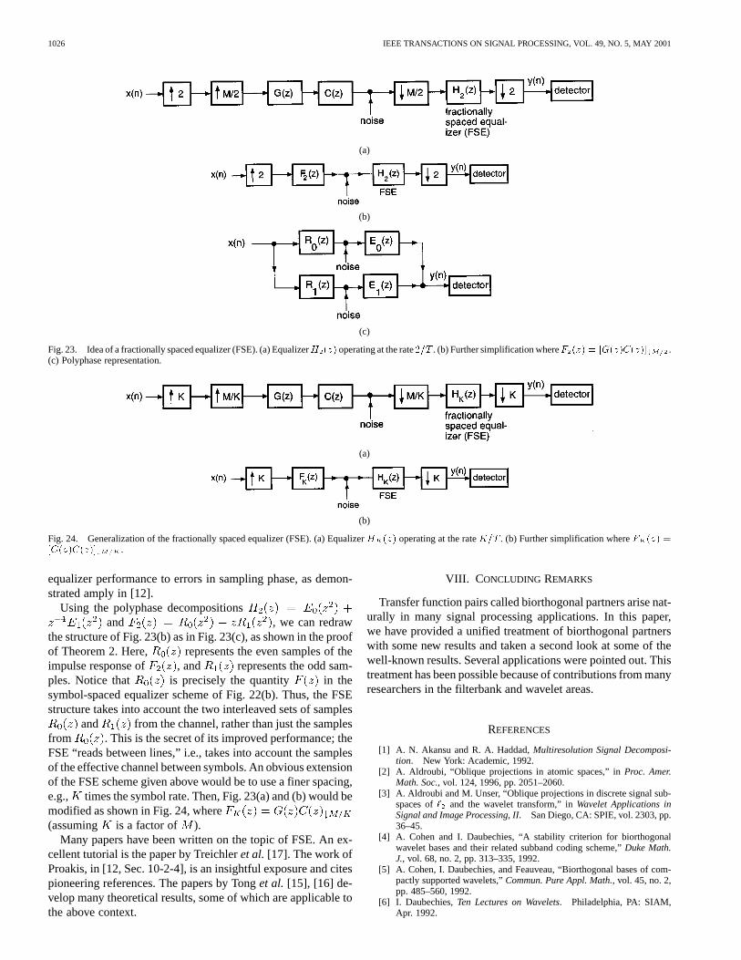
an FIR approximation. An ideal equalizer (or a zero-forcingequalizer [12]) has the form , which is IIR andtypically of high order. In real-time implementations, the idealequalizer is replaced with a practical FIR adaptive filter. It canbe shown that the ISI suppression achieved by this filter is quitesensitive to the phase of sampling at the receiver [12]. The useof a so-calledfractionally spacedequalizer (FSE) significantlyreduces this problem and, moreover, allows FIR solutions [17].

To explain what an FSE is, consider again Fig. 21. Supposethe received signal is sampled at twice the symbol rate. Wethen use an equalizer and downsample its output by 2before sending it to the detector. The system can then be rep-resented in discrete time multirate notation by Fig. 23(a) (as-suming is even). This can be simplified into the form shownin Fig. 23(b), where . (Again, thenoise source can be adjusted accordingly). We see that the ef-fective transfer function between the transmitted symbolsand received symbols is now . This can be madeunity by designing to be abiorthogonal partnerof .The filter is the fractionally spaced equalizer. It operatesat twice the symbol rate. Typically, represents an FIR ap-proximation of . Thus, according to Theorem 2,it is almost always possible to find anFIR equalizer , theonly mild condition being that the two polyphase componentsof be coprime. The FSE technique not only offers an FIRsolution, but it also reduces significantly the sensitivity of the


(a)

(b)

(c)

Fig. 23. Idea of a fractionally spaced equalizer (FSE). (a) EqualizerH (z) operating at the rate2=T . (b) Further simplification whereF (z) = [G(z)C(z)] .(c) Polyphase representation.

(a)

(b)

Fig. 24. Generalization of the fractionally spaced equalizer (FSE). (a) EqualizerH (z) operating at the rateK=T . (b) Further simplification whereF (z) =[G(z)C(z)] .

equalizer performance to errors in sampling phase, as demon-strated amply in [12].

Using the polyphase decompositionsand , we can redraw

the structure of Fig. 23(b) as in Fig. 23(c), as shown in the proofof Theorem 2. Here, represents the even samples of theimpulse response of , and represents the odd sam-ples. Notice that is precisely the quantity in thesymbol-spaced equalizer scheme of Fig. 22(b). Thus, the FSEstructure takes into account the two interleaved sets of samples

and from the channel, rather than just the samplesfrom . This is the secret of its improved performance; theFSE “reads between lines,” i.e., takes into account the samplesof the effective channel between symbols. An obvious extensionof the FSE scheme given above would be to use a finer spacing,e.g., times the symbol rate. Then, Fig. 23(a) and (b) would bemodified as shown in Fig. 24, where(assuming is a factor of ).

Many papers have been written on the topic of FSE. An ex-cellent tutorial is the paper by Treichleret al. [17]. The work ofProakis, in [12, Sec. 10-2-4], is an insightful exposure and citespioneering references. The papers by Tonget al. [15], [16] de-velop many theoretical results, some of which are applicable tothe above context.

VIII. C ONCLUDING REMARKS

Transfer function pairs called biorthogonal partners arise nat-urally in many signal processing applications. In this paper,we have provided a unified treatment of biorthogonal partnerswith some new results and taken a second look at some of thewell-known results. Several applications were pointed out. Thistreatment has been possible because of contributions from manyresearchers in the filterbank and wavelet areas.

REFERENCES

[1] A. N. Akansu and R. A. Haddad,Multiresolution Signal Decomposi-tion. New York: Academic, 1992.

[2] A. Aldroubi, “Oblique projections in atomic spaces,” inProc. Amer.Math. Soc., vol. 124, 1996, pp. 2051–2060.

[3] A. Aldroubi and M. Unser, “Oblique projections in discrete signal sub-spaces of and the wavelet transform,” inWavelet Applications inSignal and Image Processing, II. San Diego, CA: SPIE, vol. 2303, pp.36–45.

[4] A. Cohen and I. Daubechies, “A stability criterion for biorthogonalwavelet bases and their related subband coding scheme,”Duke Math.J., vol. 68, no. 2, pp. 313–335, 1992.

[5] A. Cohen, I. Daubechies, and Feauveau, “Biorthogonal bases of com-pactly supported wavelets,”Commun. Pure Appl. Math., vol. 45, no. 2,pp. 485–560, 1992.

[6] I. Daubechies,Ten Lectures on Wavelets. Philadelphia, PA: SIAM,Apr. 1992.


[7] C. de Boor,A Practical Guide to Splines. New York: Springer-Verlag,1978.

[8] I. Djokovic and P. P. Vaidyanathan, “Generalized sampling theorems inmultiresolution subspaces,”IEEE Trans. Signal Processing, vol. 45, pp.583–599, Mar. 1997.

[9] S. Mallat, “A theory for multiresolution signal decomposition: thewavelet representation,”IEEE Trans. Pattern Anal. Machine Intell.,vol. 11, pp. 674–693, July 1989.

[10] , A Wavelet Tour of Signal Processing. New York: Academic,1998.

[11] A. V. Oppenheim, A. S. Willsky, and I. T. Young,Signals and Sys-tems. Englewood Cliffs, NJ: Prentice-Hall, 1983.

[12] J. G. Proakis,Digital Communications. New York: McGraw-Hill,1995.

[13] I. J. Schoenberg,Cardinal Spline Interpolation. Philadelphia, PA:SIAM, 1973.

[14] M. G. Strintzis, “Optimal pyramidal and subband decompositions forhierarchical coding of noisy and quantized images,”IEEE Trans. ImageProcessing, vol. 7, pp. 155–166, Feb. 1998.

[15] L. Tong, G. Xu, and T. Kailath, “Blind identification and equalizationbased on second order statistics: A time domain approach,”IEEE Trans.Inform. Theory, vol. 40, pp. 340–349, Mar. 1994.

[16] , “Blind identification and equalization based on second order sta-tistics: A frequency domain approach,”IEEE Trans. Inform. Theory, vol.41, pp. 329–334, Jan. 1995.

[17] J. R. Treichler, I. Fijalkow, and C. R. Johnson, Jr., “Fractionally spacedequalizers: How long should they really be?,”IEEE Signal ProcessingMag., pp. 65–81, May 1996.

[18] M. Unser and A. Aldroubi, “Polynomial splines and wavelets,” inWavelets, A Tutorial in Theory and Applications, C. K. Chui, Ed. NewYork: Academic, 1992.

[19] M. Unser, A. Aldroubi, and M. Eden, “Fast B-spline transforms for con-tinuous image representation and interpolation,”IEEE Trans. PatternAnal. Machine Intell., vol. 10, pp. 277–285, Mar. 1991.

[20] , “B-spline signal processing–Part I: Theory,”IEEE Trans. SignalProcessing, vol. 41, pp. 821–833, Feb. 1993.

[21] , “B-spline signal processing–Part II: Efficient design and applica-tions,” IEEE Trans. Signal Processing, vol. 41, pp. 834–848, Feb. 1993.

[22] M. Unser, “Sampling—50 years after Shannon,”Proc. IEEE, vol. 88,pp. 569–587, Apr. 2000.

[23] P. P. Vaidyanathan,Multirate Systems and Filter Banks. EnglewoodCliffs, NJ: Prentice-Hall, 1993.

[24] P. P. Vaidyanathan and I. Djokovic, “Wavelet transforms,” inThe Cir-cuits and Filters Handbook, W. K. Chen, Ed. Boca Raton, FL: CRC,1995, pp. 134–219.

[25] P. P. Vaidyanathan and S.-M. Phoong, “Reconstruction of sequencesfrom nonuniform samples,” inProc. IEEE Int. Symp. Circuits Syst.,Seattle, WA, Apr.–May 1995.

[26] , “Discrete time signals which can be recovered from samples,” inProc. IEEE Int. Conf. Acoust. Speech, Signal Process., Detroit, MI, May1995.

[27] M. Vetterli and J. Kovacevic, Wavelets and SubbandCoding. Englewood Cliffs, NJ: Prentice-Hall, 1995.

[28] G. G. Walter, “A sampling theorem for wavelet subspaces,”IEEE Trans.Inform. Theory, vol. 38, pp. 881–884, Mar. 1992.

P. P. Vaidyanathan(S’80–M’83–SM’88–F’91) wasborn in Calcutta, India, on October 16, 1954. Hereceived the B.Sc. (Hons.) degree in physics and theB.Tech. and M.Tech. degrees in radiophysics andelectronics, all from the University of Calcutta, in1974, 1977, and 1979, respectively, and the Ph.D.degree in electrical and computer engineering fromthe University of California, Santa Barbara (UCSB),in 1982.

He was a Post Doctoral Fellow at UCSB fromSeptember 1982 to March 1983. In March 1983,

he joined the Electrical Engineering Department, California Institute ofTechnology (Caltech), Pasadena, as an Assistant Professor, and since 1993, hehas been Professor of Electrical Engineering. His main research interests arein digital signal processing, multirate systems, wavelet transforms, and signalprocessing for digital communications.

Dr. Vaidyanathan served as Vice Chairman of the Technical Program Com-mittee for the 1983 IEEE International Symposium on Circuits and Systemsand as the Technical Program Chairman for the 1992 IEEE International Sym-posium on Circuits and Systems. He was an Associate Editor for the IEEETRANSACTIONS ONCIRCUITS AND SYSTEMSfrom 1985 to 1987 and is currentlyan Associate Editor for the IEEE SIGNAL PROCESSINGLETTERS and a Con-sulting Editor for the journalApplied and Computational Harmonic Analysis.He was a Guest Editor in 1998 for special issues of the IEEE TRANSACTIONS ON

SIGNAL PROCESSINGand the IEEE TRANSACTIONS ONCIRCUITS AND SYSTEMS

II, on the topics of filterbanks, wavelets, and subband coders. He has authoreda number of papers in IEEE journals and is the author of the bookMultirateSystems and Filter Banks(Englewood Cliffs, NJ: Prentice-Hall, 1993). He haswritten several chapters for various signal processing handbooks. He was a re-cipient of the Award for Excellence in Teaching at the Caltech in 1983–1984,1992–1993, and 1993–1994. He received the National Science Foundation Pres-idential Young Investigator award in 1986. In 1989, he received the IEEE ASSPSenior Award for his paper on multirate perfect-reconstruction filter banks. In1990, he was recipient of the S. K. Mitra Memorial Award from the Instituteof Electronics and Telecommunications Engineers, India, for his joint paper inthe IETE journal. He was also the coauthor of a paper on linear-phase perfectreconstruction filter banks in the IEEE TRANSACTIONS ONSIGNAL PROCESSING,for which the first author (T. Nguyen) received the Young Outstanding Au-thor award in 1993. He received the 1995 F. E. Terman Award of the Amer-ican Society for Engineering Education, sponsored by Hewlett Packard Co., forhis contributions to engineering education, especially the bookMultirate Sys-tems and Filter Banks. He has given several plenary talks at the Eusipco’98,Asimolar’88, and SPCOM’95 conferences on signal processing. He has beenchosen a Distinguished Lecturer for the IEEE Signal Processing Society for theyear 1996–1997. In 1999, he was chosen to receive the IEEE Circuits and Sys-tems Society’s Golden Jubilee Medal.

Bojan Vrcelj (S’99) was born in Belgrade, Yu-goslavia, in 1974. He received the B.S. degree fromthe University of Belgrade in 1998 and the M.S.degree from the California Institute of Technology(Caltech), Pasadena, in 1999, both in electricalengineering. In 1998, he received the GraduateDivision Fellowship from Caltech. He is currentlypursuing the Ph.D. degree in the field of digitalsignal processing at Caltech.

His research interests include multirate systems,wavelets and their applications in digital communi-

cations, as well as image processing and interpolation.

Documents

Biorthogonal partners and applications - Signal Processing ... · Biorthogonal Partners and Applications P. P. Vaidyanathan, Fellow, IEEE, and Bojan Vrcelj, Student Member, IEEE Abstract—