Biophysical Techniques (BPHS 4090/PHYS 5800)

York University Winter 2017 Lec.8

Instructors: Prof. Christopher Bergevin (cberge@yorku.ca)

Schedule: MWF 1:30-2:30 (CB 122)

Website: http://www.yorku.ca/cberge/4090W2017.html

Note(readdi+onalusefulref.)h4p://www.robots.ox.ac.uk/~az/lectures/ia/lect2.pdf

GoalDevelopknowledgeandintui+ondealingw/2DFouriertransforms

2-Dcase(e.g.,image)

0 1 2 3 4 5 6 7 8−1

−0.8

−0.6

−0.4

−0.2

0

0.2

0.4

0.6

0.8

1

Time [s]

Pres

sure

[arb

]

time waveform

‘+mewaveform’recordedfrommic

Recall:1-Dcase

2-DFourieranalysis

Note:Independentvariables(xandyhere)canrepresentanyphysicalquan+ty,butfor2-Dwetypicallyuseposi+oninCartesianplane(ratherthan+me)

Fouriertransform

InverseFouriertransform

Hobbie&Roth

2-D

1-D

Othernota+onreFourieranalysis

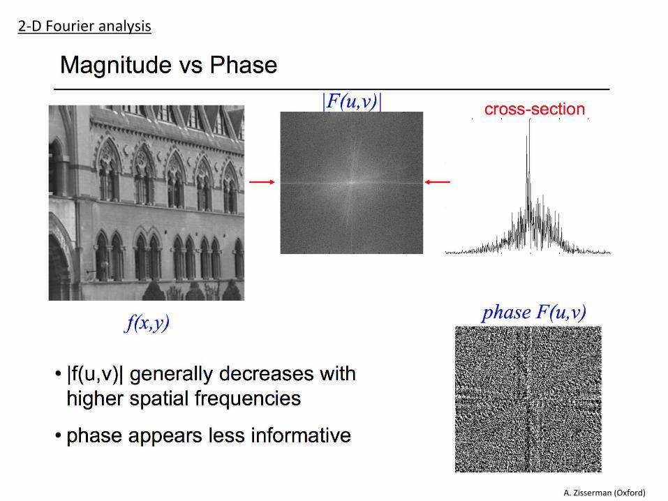
A.Zisserman(Oxford)

2-DFourieranalysis

EX2DfourierGra+ng.m% ### EX2DfourierGrating.m ### 2013.09.15 CB (updated 2017.01.20)! !clear!% ==========================================================!type= 0; % boolean to switch between sine (0) and boxcar (1) gratings!imSize = 400; % image size: n X n {200}!lamda = 15; % wavelength (number of pixels per cycle) {20}!theta = -45; % grating orientation [deg] {-140}!phase = 0; % offset phase [cycles] {0}!mScale= 1; % boolean re linear (0) or log (1) axes for the magnitude {1}!% ==========================================================! !% ---!% make the grating!X = 1:imSize; % X is a vector from 1 to imageSize!X0 = (X / imSize) - .5; % rescale X -> -.5 to .5!sinX = sin(X0 * 2*pi); % convert to radians and do sine!freq = imSize/lamda; % compute frequency from wavelength!Xf = X0 * freq * 2*pi; % convert X to radians: 0 -> ( 2*pi * frequency)!sinX = sin(Xf) ; % make new sinewave!phaseRad = (phase * 2* pi); % convert to radians: 0 -> 2*pi!sinX = sin( Xf + phaseRad) ; % make phase-shifted sinewave!% now put the basic grating together![Xm Ym] = meshgrid(X0, X0); % 2D matrices!Xf = Xm * freq * 2*pi;!grating = sin( Xf + phaseRad); % make 2D sinewave!% ---!% deal w/ rotation!thetaRad = (theta / 360) * 2*pi; % convert theta (orientation) to radians!Xt = Xm * cos(thetaRad); % compute proportion of Xm for given orientation!Yt = Ym * sin(thetaRad); % compute proportion of Ym for given orientation!XYt = [ Xt + Yt ]; % sum X and Y components!XYf = XYt * freq * 2*pi; % convert to radians and scale by frequency!grating = sin( XYf + phaseRad); % make 2D sinewave!% ---!% convert to boxcar (i.e., everything is rounded to 0 or 1) if specified!if (type==1), grating= round((grating+1)/2); end!imageA= grating;!% ---!fftA = fft2((imageA)); % compute FFT!% places zero-frequency position in center?!if (1==1), FA= fftshift(fftA); else FA= fftA; end!

% ---!figure(1); clf;!subplot(221); imagesc(imageA); title('Image A'); colorbar;!if mScale==0! subplot(223); imagesc(abs(FA),[0 100000]); colormap gray; title('Mag.'); colorbar; % linear axes!else! subplot(223); imagesc(db(FA)); colormap gray; title('Mag.'); colorbar; % log axes!end!subplot(224); imagesc(angle(FA),[-pi pi]); colormap gray; title('Phase'); colorbar;!xlabel('Freq. scale incorrect')! !% ---!% make another plot ignoring redundant info; separating that info is!% handled here in a bit of a kludge way!specU= fftshift(fftA,1); %use fftshift to better line up relevant bit!specU= specU(:,1:ceil(end/2)); % ignore redundant info!specU= rot90(specU); specU= fliplr(specU); % rotate/flip to correctly(?) line things up!figure(2); clf;!specU= padarray(specU,[5 5],'both'); % pad some zeros around so to better see on-axis values!subplot(211); imagesc(dB(specU)); colormap jet; colorbar; title('Magnitude'); !xlabel('y'); ylabel('x (axis label is wrongly flipped)'); title('Coords rotated 90 deg'); !subplot(212); imagesc(angle(specU)); colormap jet; colorbar; title('Phase'); !xlabel('y (freq. scale incorrect)'); ylabel('x');!

EX2DfourierGra+ng.mlamda = 15; % wavelength (number of pixels per cycle)!theta = -45; % grating orientation [deg]!

EX2DfourierGra+ng.m

colormap jet!

EX2DfourierGra+ng.mlamda = 5; % wavelength (number of pixels per cycle)!theta = 45; % grating orientation [deg]!

EX2DfourierGra+ng.mlamda = 25; % wavelength (number of pixels per cycle)!theta = 0; % grating orientation [deg]!

A.Zisserman(Oxford)

Note:Only½oftheinforma+onisbeingshownforthespectraldomain(i.e.,justthemagnitude)

2-DFourieranalysis

Hobbie&Roth

Spectraldomain Spa+aldomain

Note:Only½oftheinforma+onisbeingshownforthespectraldomain(i.e.,justthemagnitude)

2-DFourieranalysis

Reminder:Hobbie&Rothsome+mesexpressviathesine&cosinetransforms

Hobbie&Roth

Reminder:Hobbie&Rothsome+mesexpressviathesine&cosinetransforms....

...butcomplexexponen+alsworkfine(be4er?)too

Othernota+onreFourieranalysis

EX2Dfourier1.m% ### EX2Dfourier1.m ### 2015.09.15 CB (updated 2017.01.20)! !% Read in an image and compute the 2D FFT, plotting both mag and phase; can!% also rotate the image 90! !% Notes!% o Caution: axes for FFT are not (presently) properly labeled! !% Source:basic syntax borrowed from "How to Do a 2-D Fourier Transform in Matlab"!% http://matlabgeeks.com/tips-tutorials/how-to-do-a-2-d-fourier-tr...! !clear!% =================================!fileA= './Images/moustacheB'; % [no need for extension]!mScale= 1; % boolean re linear (0) or log (1) axes for the magnitude!rotateI= 0; % boolean to rotate image CCW 90 deg {0}!flipI= 0; % boolean to flip image about vertical {0}!% =================================!% ---!imageA = imread(fileA,'jpg'); % load in an image!% ---!% various possible manipulations!if (size(imageA,3)>1), imageA= rgb2gray(imageA); end % if color, convert to B&W!if (rotateI==1), imageA= rot90(imageA); end % rotate!if (flipI==1), imageA= fliplr(imageA); end % flip!% ---!fftA = fft2((imageA)); % compute FFT!% ---!% places zero-frequency position in center?!if (1==1), FA= fftshift(fftA); else FA= fftA; end!% ---!% plot!figure(1); clf;!subplot(221); imagesc(imageA); title('Image'); colorbar; xlabel('Pixel # (x)'); ylabel('Pixel # (y)');!if mScale==0! subplot(223); imagesc(abs(FA),[0 100000]); colormap gray; title('Mag.'); colorbar; % linear axes!else! subplot(223); imagesc(dB(FA)); colormap gray; title('Mag.'); colorbar; % log axes!end!subplot(224); imagesc(angle(FA),[-pi pi]); colormap gray; title('Phase'); colorbar;!xlabel('Freq. scale incorrect’)!

EX2Dfourier1.m

EX2Dfourier1.m

A.Zisserman(Oxford)

àDidwegetthesameresult?

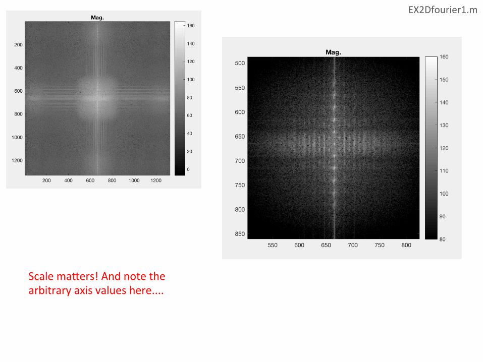
EX2Dfourier1.m

Scalema4ers!Andnotethearbitraryaxisvalueshere....

EX2Dfourier2.m% ### EX2Dfourier2.m ### 2017.01.20 CB! !% Variation on EX2Dfourier1.m to draw attention to role that fftshift.m plays!% and the redundant information that is displayed (due to symmetry, given!% that the image is real-valued)! !clear!% =================================!fileA= './Images/moustacheB'; % [no need for extension]!mScale= 1; % boolean re linear (0) or log (1) axes for the magnitude!rotateI= 0; % boolean to rotate image CCW 90 deg {0}!flipI= 0; % boolean to flip image about vertical {0}!% =================================!% ---!imageA = imread(fileA,'jpg'); % load in an image!% ---!% various possible manipulations!if (size(imageA,3)>1), imageA= rgb2gray(imageA); end % if color, convert to B&W!if (rotateI==1), imageA= rot90(imageA); end % rotate!if (flipI==1), imageA= fliplr(imageA); end % flip!% ---!fftA = fft2((imageA)); % compute FFT!% ---!fftB= fftshift(fftA); % places zero-frequency position in center?!% ---!% plot!fig1= figure(1); clf;!subplot(221); imagesc(imageA); title('Image'); colorbar; xlabel('Pixel # (x)'); ylabel('Pixel # (y)');!subplot(223); imagesc(dB(fftA)); colormap gray; title('Mag. (No shift)'); colorbar; % log axes!subplot(224); imagesc(dB(fftB)); colormap gray; title('Mag. (Shifted)'); colorbar; % log axes!xlabel('Freq. scale incorrect')!% ---!% make another plot ignoring redundant info; separating that info is!% handled here in a bit of a kludge way!specU= fftshift(fftA,1); %use fftshift to better line up relevant bit!specU= specU(:,1:ceil(end/2)); % ignore redundant info!specU= rot90(specU); specU= fliplr(specU); % rotate/flip to correctly(?) line things up!figure(2); clf;!subplot(211); imagesc(dB(specU)); colormap(jet); colorbar; title('Magnitude');!subplot(212); imagesc(angle(specU)); colormap(jet); colorbar; title('Phase'); xlabel('Freq. scale incorrect')!% ---!% print some info to screen!if 1==0! disp(['For the "shifted" version (via fftshift.m),','the zero frequncy appears in the center.'])! disp(['For the non-shifted version, positive','frequncies start at 0 in the bottom left'])! disp(['corner and increase as you move','right (x) and up (y). Note that half the info']);! disp(['here is redundant though.']);!end!

EX2Dfourier2.m

EX2Dfourier2.m

àMosteffec+vewaytogetridofredundantinfo?

Connec+onPoint:X-rayCrystallography

Candes et al (2015)

Ø  Verycommonmethodologyusedtodeterminemolecularstructure

Ø  Diffrac+onpa4ernistheFouriertransform

Ø  However,onlymagnitudeinforma+onispreserved(!)

àWe’llreturntothislaterinthesemester....

A.Zisserman(Oxford)

2-DFourieranalysis

A.Zisserman(Oxford)

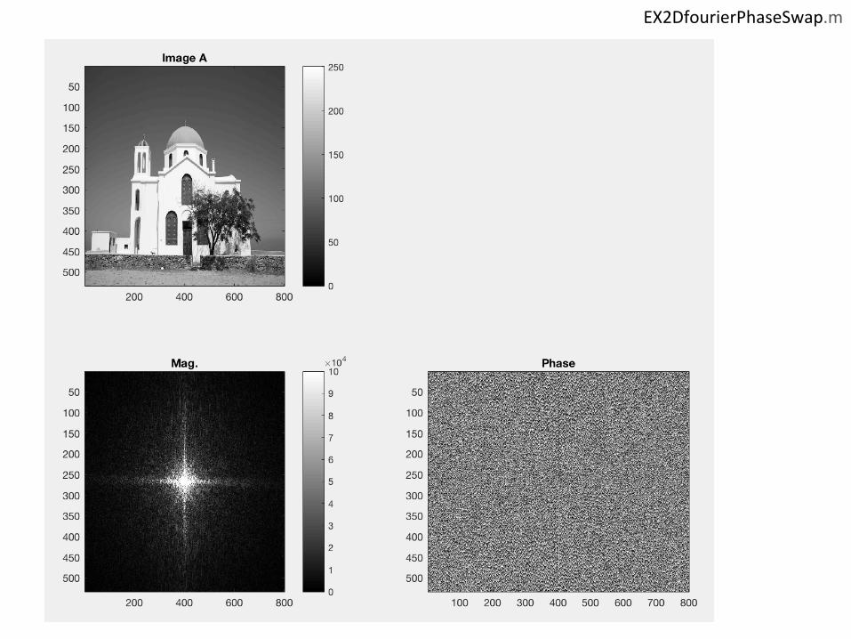
Swapphases,theninversetransformtogettheimageback

2-DFourieranalysis

EX2DfourierPhaseSwap.m% ### EX2DfourierPhaseSwap.m ### 2015.09.11 CB (updated 2017.01.20)! !clear!% ==========================================================!fileA= './Images/GreekChurch'; % [no need for extension]!fileB= './Images/moustacheB';!mScale= 0; % boolean re linear (0) or log (1) axes for the magnitude!% ==========================================================!% ---!% load in images!imageA = imread(fileA,'jpg'); % load in an image!imageB = imread(fileB,'jpg'); !% ---!% if color, convert to B&W!if size(imageA,3)>1! imageA= rgb2gray(imageA);! imageB= rgb2gray(imageB);!end!% ---!% compute FFT!fftA = fft2((imageA));!fftB = fft2((imageB));!% places zero-frequency position in center?!if (1==1), FA= fftshift(fftA); FB= fftshift(fftB); else FA= fftA; FB= fftB; end!% ---!% plot originals + 2D FFT!figure(1); clf;!subplot(221); imagesc(imageA); title('Image A'); colorbar;!if mScale==0! subplot(223); imagesc(abs(FA),[0 100000]); colormap gray; title('Mag.'); colorbar; % linear axes!else! subplot(223); imagesc(db(FA)); colormap gray; title('Mag.'); colorbar; % log axes!end!subplot(224); imagesc(angle(FA),[-pi pi]); colormap gray; title('Phase')!figure(2); clf;!subplot(221); imagesc(imageB); title('Image B'); colorbar;!if mScale==0! subplot(223); imagesc(abs(FB),[0 100000]); colormap gray; title('Mag.'); colorbar; % linear axes!else! subplot(223); imagesc(db(FB)); colormap gray; title('Mag.'); colorbar; % log axes!end!subplot(224); imagesc(angle(FB),[-pi pi]); colormap gray; title('Phase')!xlabel('Freq. scale incorrect')!% ---!% swap mag and phases from both images!fftC = abs(fftA).*exp(i*angle(fftB));!fftD = abs(fftB).*exp(i*angle(fftA));!imageC = ifft2(fftC);!imageD = ifft2(fftD);!cmin = min(min(abs(imageC))); cmax = max(max(abs(imageC)));!dmin = min(min(abs(imageD))); dmax = max(max(abs(imageD)));!% ---!figure(3); clf; hold on;!subplot(221); imagesc(abs(imageC), [cmin cmax]); colormap gray; title('Im.A Mag. + Im.B Phase')!subplot(223); imagesc(abs(imageD), [dmin dmax]); colormap gray; title('Im.B Mag. + Im.A Phase')! !

EX2DfourierPhaseSwap.m

EX2DfourierPhaseSwap.m

EX2DfourierPhaseSwap.m

How does Photoshop “work”? (at least in very basic terms)

Convolu+ons(Revisited)

A. Zisserman (Oxford)

Devries (1994)

Ø  Proof:ConsidertheFouriertransformofthe(1-D)convolu+on:

Ø  Makinguseofthe‘shibingproperty’,theterminthesquarebracketsis:

Q(ω) istheFouriertransformof q(t)

P(ω)istheFouriertransformof p(t)

Convolution theorem

Convolu+ons&(1-D)FourierTransforms

Convolu+ons&(2-D)FourierTransforms

Hobbie&Roth

Ø  Soaconvolu+onisabitmessyinthespa+aldomain....

Wikipedia [see page for Kernel (image processing)]

Convolu+onàSharpening

Basicideaisthataconvolu+onisanumericalopera+onbetweenimageandkernel

Review

Convolu+ons&(2-D)FourierTransforms

Hobbie&Roth

Ø  Soaconvolu+onisabitmessyinthespa+aldomain....

Ø  ....butissimplyamul+plica+oninthespectraldomain(easy!)

EX2DfourierBlur.m% ### EX2DfourierBlur.m ### 2015.29.11 CB (updated 2017.01.20)! !% By creating a "blurring" impulse response, the purpose is to perform a !% convolution (in the spectral domain, i.e., via a multiplication) to blur!% an image! !clear!% ==========================================================!fileA= './Images/HRfig12x6'; % [no need for extension]!mScale= 0; % boolean re linear (0) or log (1) axes for the magnitude!sigma= 10; % width for blurring kernel!% ==========================================================!% ---!imageA = imread(fileA,'jpg'); % load in an image!% ---!% if color, convert to B&W!if (size(imageA,3)>1), imageA= rgb2gray(imageA); end!% ---!fftA = fft2((imageA)); % compute FFT!% ---!% create (spectral) impulse response![dimx dimy]= size(imageA); % get the correct dimensions![X,Y]=meshgrid(1:dimx,1:dimy); % create baseline mesh!impulse= (1000/sqrt(2*pi).*exp(-((X-dimx/2).^2/(2*sigma^2))-((Y-dimy/2).^2/(2*sigma^2))));!impulse= impulse/(max(max(impulse))); % normalize to unity!filter= fft2((impulse)); % convert to spectral domain!% ---!% convolve by multiplying in the freq. domain!blurredS= fftA.*filter;!% ---!% inverse transform back!imageF= ifft2(blurredS, 'symmetric');!imageF= fftshift(imageF); % Kludge (need to reshift; unsure why...)!% ---!% places zero-frequency position in center?!if (1==1), FA= fftshift(filter); else FA= filter; end!% ---!% plot!figure(1); clf;!subplot(221); imagesc(imageA); title('Image A'); colorbar; % original!subplot(222); imagesc(imageF); title('Convolved version'); colorbar;!subplot(223); imagesc(impulse); colormap gray; title('PSF (spatial)'); colorbar;!if mScale==0! subplot(224); imagesc(abs(FA)); title('PSF (spectral; mag.)'); colorbar; % linear axes!else! subplot(224); imagesc(db(FA)); title('PSF (spectral; mag.)'); colorbar; % log axes!end!xlabel('Freq. scale incorrect')!

EX2DfourierBlur.m

FilteringàIntui+onabouthowspectralcontentrelatesbacktowhatwesee

Low-pass

High-pass

Wikipedia

Note:Wehavenotyetdevelopedaclearintui+onforwhataconvolu1onis...

àWewillreturntotheseinterrela+onships(in1-D)shortly...