Embed Size (px)
Citation preview
ACL 2013
BioNLP 2013
2013 Workshop on Biomedical Natural Language Processing
Proceedings of the Workshop
August 8, 2013Sofia, Bulgaria
Production and Manufacturing byOmnipress, Inc.2600 Anderson StreetMadison, WI 53704 USA
Sponsored by the Computational Medicine Center and Division of Biomedical Informatics, CincinnatiChildren’s Hospital Medical Center
c©2013 The Association for Computational Linguistics
Order copies of this and other ACL proceedings from:
Association for Computational Linguistics (ACL)209 N. Eighth StreetStroudsburg, PA 18360USATel: +1-570-476-8006Fax: [email protected]
ISBN 978-1-937284-54-1
ii
Introduction
BioNLP 2013 has accepted 11 outstanding full papers and five posters. The themes in this year’s papersand posters are divided equally between clinical and biomedical text processing. In addition to thecustomary research in practical and theoretical issues, such as domain adaptation, question answering,temporal relations extraction, and evaluation of text mining methods, this year, we see a growing bodyof research in languages other than English. The issues with clinical text processing in resource-poorlanguages are also discussed in the keynote presentation.
Keynote: Processing clinical narratives in less-resourced languages: the challenge to start from scratch
Galia Angelova, Ph.D. Linguistic Modeling Department, Institute of Information and CommunicationTechnologies, Bulgarian Academy of Sciences
Dr. Angelova presents automatic analysis of free texts in Bulgarian hospital discharge letters of patientswith endocrine and metabolic diseases. Processing Bulgarian clinical texts is challenging due tosome specific reasons: the notes contain about 37% Latin terms that might occur in Latin alphabetcharacters as well as transliterated to Cyrillic alphabet (34% of all tokens); the lack of importantmedical nomenclatures in Bulgarian: for example, the ATC classification is supported in Latin only andrequires manual augmentation with Bulgarian drug names in Cyrillic alphabet; no electronic resourcewith medical terminology is available so the collection of terms and important phrases involves analysisof documents, such as manuals for coding to ICD-10 terms, or collection of collocations directly from thecorpus of discharge letters, among others. Currently available resources and methods include automaticrecognition of ICD-10 diagnoses; drugs, especially those taken during hospitalization; patient status;values of laboratory tests; and the temporal structure of diabetic case histories. Dr. Angelova discussesscenarios for application of the extraction components in practical settings when cleaning and validationof patient data is required.
Dr. Claire Nedellec presents an overview of the BioNLP Shared Task 2013.
Acknowledgments
We are profoundly grateful to the authors who chose BioNLP as venue for presenting their innovativeresearch. The authors’ willingness to share their work through BioNLP consistently makes the workshopnoteworthy among the increasing numbers of available venues. We are equally indebted to the programcommittee members (listed elsewhere in this volume) who produced at least three thorough reviews perpaper on a tight review schedule and with an admirable level of insight. Finally, we acknowledge thegracious sponsorship of the Computational Medicine Center and Division of Biomedical Informatics,Cincinnati Children’s Hospital Medical Center.
iii

Organizers:
Kevin Bretonnel Cohen, University of Colorado School of MedicineDina Demner-Fushman, US National Library of MedicineSophia Ananiadou, University of Manchester and National Centre for Text Mining, UKJohn Pestian, Computational Medical Center, University of Cincinnati,Cincinnati Children’s Hospital Medical CenterJun’ichi Tsujii, Microsoft Research Asiaand National Centre for Text Mining, UK
Program Committee:
Emilia Apostolova, DePaul University, USAEiji Aramaki, University of Tokyo, JapanAlan Aronson, US National Library of MedicineSabine Bergler, Concordia University, CanadaOlivier Bodenreider, US National Library of MedicineKevin Cohen, University of Colorado, USANigel Collier, National Institute of Informatics, JapanDina Demner-Fushman, US National Library of MedicineNoemie Elhadad, Columbia University, USAMarcelo Fiszman, US National Library of MedicineFilip Ginter, University of Turku, FinlandGraciela Gonzalez, Arizona State University, USAAntonio Jimeno Yepes, NICTA, AustraliaHalil Kilicoglu, US National Library of MedicineJin-Dong Kim, University of Tokyo, JapanRobert Leaman, US National Library of MedicineUlf Leser, Humboldt University of Berlin, GermanyZhiyong Lu, US National Library of MedicineMakoto Miwa, National Centre for Text Mining, UKNaoaki Okazaki, Tohoku University, JapanJong Park, KAIST, South KoreaRashmi Prasad, University of Wisconsin-Milwaukee, USASampo Pyysalo, National Centre for Text Mining, UKBastien Rance, Georges Pompidou European Hospital, FranceAndrey Rzhetsky, University of Chicago, USAMatthew Simpson, US National Library of MedicinePontus Stenetorp, University of Tokyo, JapanYoshimasa Tsuruoka, University of Tokyo, JapanKarin Verspoor, NICTA, AustraliaW. John Wilbur, US National Library of MedicinePierre Zweigenbaum, LIMSI, France
Invited Speakers:Galia Angelova, Bulgarian Academy of SciencesProcessing clinical narratives in less-resourced languages: the challenge to start from scratchClaire Nedellec, INRAOverview of the BioNLP Shared Task 2013
v

Table of Contents
Earlier Identification of Epilepsy Surgery Candidates Using Natural Language ProcessingPawel Matykiewicz, Kevin Cohen, Katherine D. Holland, Tracy A. Glauser, Shannon M. Stan-
dridge, Karen M. Verspoor and John Pestian . . . . . . . . . . . . . . . . . . . . . . . . . . . . . . . . . . . . . . . . . . . . . . . . . . . . . 1
Identification of Patients with Acute Lung Injury from Free-Text Chest X-Ray ReportsMeliha Yetisgen-Yildiz, Cosmin Bejan and Mark Wurfel . . . . . . . . . . . . . . . . . . . . . . . . . . . . . . . . . . . .10
Discovering Temporal Narrative Containers in Clinical TextTimothy Miller, Steven Bethard, Dmitriy Dligach, Sameer Pradhan, Chen Lin and Guergana Savova
18
Identifying Pathological Findings in German Radiology Reports Using a Syntacto-semantic Parsing Ap-proach
Claudia Bretschneider, Sonja Zillner and Matthias Hammon . . . . . . . . . . . . . . . . . . . . . . . . . . . . . . . . 27
Corpus-Driven Terminology Development: Populating Swedish SNOMED CT with Synonyms Extractedfrom Electronic Health Records
Aron Henriksson, Maria Skeppstedt, Maria Kvist, Martin Duneld and Mike Conway . . . . . . . . . . 36
Unsupervised Linguistically-Driven Reliable Dependency Parses Detection and Self-Training for Adap-tation to the Biomedical Domain
Felice Dell’Orletta, Giulia Venturi and Simonetta Montemagni . . . . . . . . . . . . . . . . . . . . . . . . . . . . . . 45
Interpreting Consumer Health Questions: The Role of Anaphora and EllipsisHalil Kilicoglu, Marcelo Fiszman and Dina Demner-Fushman. . . . . . . . . . . . . . . . . . . . . . . . . . . . . . .54
Evaluating Large-scale Text Mining Applications Beyond the Traditional Numeric Performance Mea-sures
Sofie Van Landeghem, Suwisa Kaewphan, Filip Ginter and Yves Van de Peer . . . . . . . . . . . . . . . . . 63
Recognizing Sublanguages in Scientific Journal Articles through Closure PropertiesIrina Temnikova and Kevin Cohen . . . . . . . . . . . . . . . . . . . . . . . . . . . . . . . . . . . . . . . . . . . . . . . . . . . . . . . . 72
BEL Networks Derived from Qualitative Translations of BioNLP Shared Task AnnotationsJuliane Fluck, Alexander Klenner, Sumit Madan, Sam Ansari, Tamara Bobic, Julia Hoeng, Martin
Hofmann-Apitius and Manuel Peitsch . . . . . . . . . . . . . . . . . . . . . . . . . . . . . . . . . . . . . . . . . . . . . . . . . . . . . . . . . 80
Exploring Word Class N-grams to Measure Language Development in ChildrenGabriela Ramirez-de-la-Rosa, Thamar Solorio, Manuel Montes, Yang Liu, Lisa Bedore, Elizabeth
Pena and Aquiles Iglesias . . . . . . . . . . . . . . . . . . . . . . . . . . . . . . . . . . . . . . . . . . . . . . . . . . . . . . . . . . . . . . . . . . . . 89
Adapting a Parser to Clinical Text by Simple Pre-processing RulesMaria Skeppstedt . . . . . . . . . . . . . . . . . . . . . . . . . . . . . . . . . . . . . . . . . . . . . . . . . . . . . . . . . . . . . . . . . . . . . . . 98
Using the Argumentative Structure of Scientific Literature to Improve Information AccessAntonio Jimeno Yepes, James Mork and Alan Aronson . . . . . . . . . . . . . . . . . . . . . . . . . . . . . . . . . . . . 102
Using Latent Dirichlet Allocation for Child Narrative AnalysisKhairun-nisa Hassanali, Yang Liu and Thamar Solorio . . . . . . . . . . . . . . . . . . . . . . . . . . . . . . . . . . . . 111
vii

Effect of Out Of Vocabulary Terms on Inferring Eligibility Criteria for a Retrospective Study in HebrewEHR
Raphael Cohen and Michael Elhadad . . . . . . . . . . . . . . . . . . . . . . . . . . . . . . . . . . . . . . . . . . . . . . . . . . . . 116
Parallels between Linguistics and BiologySutanu Chakraborti and Ashish Tendulkar . . . . . . . . . . . . . . . . . . . . . . . . . . . . . . . . . . . . . . . . . . . . . . . . 120
viii
Conference Program
Thursday, August 8, 2013
8:40–8:50 Opening Remarks
Session 1: Clinical text processing
8:50–9:10 Earlier Identification of Epilepsy Surgery Candidates Using Natural Language Pro-cessingPawel Matykiewicz, Kevin Cohen, Katherine D. Holland, Tracy A. Glauser, Shan-non M. Standridge, Karen M. Verspoor and John Pestian
9:10–9:30 Identification of Patients with Acute Lung Injury from Free-Text Chest X-Ray Re-portsMeliha Yetisgen-Yildiz, Cosmin Bejan and Mark Wurfel
9:30–9:50 Discovering Temporal Narrative Containers in Clinical TextTimothy Miller, Steven Bethard, Dmitriy Dligach, Sameer Pradhan, Chen Lin andGuergana Savova
9:50–10:10 Identifying Pathological Findings in German Radiology Reports Using a Syntacto-semantic Parsing ApproachClaudia Bretschneider, Sonja Zillner and Matthias Hammon
10:10–10:30 Corpus-Driven Terminology Development: Populating Swedish SNOMED CT withSynonyms Extracted from Electronic Health RecordsAron Henriksson, Maria Skeppstedt, Maria Kvist, Martin Duneld and Mike Conway
10:30–11:00 Morning coffee break
11:00–12:00 Invited Talk by Galia Angelova
12:00–12:30 BioNLP Shared Task overview by Claire Nedellec
12:30–14:00 Lunch break
ix
Thursday, August 8, 2013 (continued)
Session 2: Biomedical language processing
14:00–14:20 Unsupervised Linguistically-Driven Reliable Dependency Parses Detection and Self-Training for Adaptation to the Biomedical DomainFelice Dell’Orletta, Giulia Venturi and Simonetta Montemagni
14:20–14:40 Interpreting Consumer Health Questions: The Role of Anaphora and EllipsisHalil Kilicoglu, Marcelo Fiszman and Dina Demner-Fushman
14:40–15:00 Evaluating Large-scale Text Mining Applications Beyond the Traditional Numeric Perfor-mance MeasuresSofie Van Landeghem, Suwisa Kaewphan, Filip Ginter and Yves Van de Peer
15:00–15:20 Recognizing Sublanguages in Scientific Journal Articles through Closure PropertiesIrina Temnikova and Kevin Cohen
15:30–16:00 Afternoon coffee break
16:00–16:20 BEL Networks Derived from Qualitative Translations of BioNLP Shared Task AnnotationsJuliane Fluck, Alexander Klenner, Sumit Madan, Sam Ansari, Tamara Bobic, Julia Hoeng,Martin Hofmann-Apitius and Manuel Peitsch
16:20–16:40 Exploring Word Class N-grams to Measure Language Development in ChildrenGabriela Ramirez-de-la-Rosa, Thamar Solorio, Manuel Montes, Yang Liu, Lisa Bedore,Elizabeth Pena and Aquiles Iglesias
Poster Session (16:40–17:30)
Adapting a Parser to Clinical Text by Simple Pre-processing RulesMaria Skeppstedt
Using the Argumentative Structure of Scientific Literature to Improve Information AccessAntonio Jimeno Yepes, James Mork and Alan Aronson
Using Latent Dirichlet Allocation for Child Narrative AnalysisKhairun-nisa Hassanali, Yang Liu and Thamar Solorio
Effect of Out Of Vocabulary Terms on Inferring Eligibility Criteria for a RetrospectiveStudy in Hebrew EHRRaphael Cohen and Michael Elhadad
x

Thursday, August 8, 2013 (continued)
Parallels between Linguistics and BiologySutanu Chakraborti and Ashish Tendulkar
xi

Proceedings of the 2013 Workshop on Biomedical Natural Language Processing (BioNLP 2013), pages 1–9,Sofia, Bulgaria, August 4-9 2013. c©2013 Association for Computational Linguistics
Earlier Identification of Epilepsy Surgery Candidates Using NaturalLanguage Processing
Pawel Matykiewicz1, Kevin Bretonnel Cohen2, Katherine D. Holland1, Tracy A. Glauser1,Shannon M. Standridge1, Karin M. Verspoor3,4, and John Pestian1§
1 Cincinnati Children’s Hospital Medical Center, Cincinnati OH USA2 University of Colorado, Denver, CO
3 National ICT Australia and 4The University of Melbourne, Melbourne, Australia§corresponding author: [email protected]
Abstract
This research analyzed the clinical notesof epilepsy patients using techniques fromcorpus linguistics and machine learningand predicted which patients are can-didates for neurosurgery, i.e. have in-tractable epilepsy, and which are not.Information-theoretic and machine learn-ing techniques are used to determinewhether and how sets of clinic notesfrom patients with intractable and non-intractable epilepsy are different. The re-sults show that it is possible to predictfrom an early stage of treatment which pa-tients will fall into one of these two cate-gories based only on text data. These re-sults have broad implications for develop-ing clinical decision support systems.
1 Introduction and Significance
Epilepsy is a disease characterized by recurrentseizures that may cause irreversible brain damage.While there are no national registries, epidemiolo-gists have shown that roughly three million Amer-icans require $17.6 billion USD in care annuallyto treat their epilepsy (Epilepsy Foundation, 2012;Begley et al., 2000). Epilepsy is defined by theoccurrence of two or more unprovoked seizuresin a year. Approximately 30% of those individ-uals with epilepsy will have seizures that do notrespond to anti-epileptic drugs (Kwan and Brodie,2000). This population of individuals is said tohave intractable or drug-resistant epilepsy (Kwanet al., 2010).
Select intractable epilepsy patients are candi-dates for a variety of neurosurgical procedures thatablate the portion of the brain known to cause theseizure. On average, the gap between the ini-tial clinical visit when the diagnosis of epilepsyis made and surgery is six years. If it were pos-
sible to predict which patients should be consid-ered candidates for referral to surgery earlier in thecourse of treatment, years of damaging seizures,under-employment, and psychosocial distress maybe avoided. It is this gap that motivates this re-search.
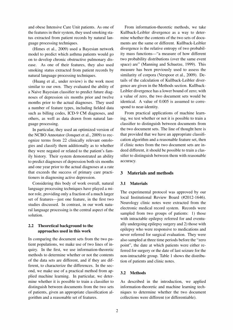
In this study, we examine the differences be-tween the clinical notes of patients early in theirtreatment course with the intent of predictingwhich patients will eventually be diagnosed as in-tractable versus which will be amenable to drug-based treatment. The null hypothesis is thatthere will be no detectable differences betweenthe clinic notes of patients who go on to a di-agnosis of intractable epilepsy and patients whodo not progress to the diagnosis of intractableepilepsy (figure 1). To further elucidate the phe-nomenon, we look at both the patient’s earli-est clinical notes and notes from a progressionof time points. Here we expect to gain insightinto how the linguistic characteristics (and natu-ral language processing-based classification per-formance) evolve over treatment course. We alsostudy the linguistic features that characterize thedifferences between the document sets from thetwo groups of patients. We anticipate that this ap-proach will ultimately be adapted for various clin-ical decision support systems.
2 Background
2.1 Related work
Although there has been extensive work on build-ing predictive models of disease progression andof mortality risk, few models take advantage ofnatural language processing in addressing thistask.
(Abhyankar et al., 2012) used univariate anal-ysis, multivariate logistic regression, sensitivityanalyses, and Cox proportional hazards models topredict 30-day and 1-year survival of overweight
1
and obese Intensive Care Unit patients. As one ofthe features in their system, they used smoking sta-tus extracted from patient records by natural lan-guage processing techniques.
(Himes et al., 2009) used a Bayesian networkmodel to predict which asthma patients would goon to develop chronic obstructive pulmonary dis-ease. As one of their features, they also usedsmoking status extracted from patient records bynatural language processing techniques.
(Huang et al., under review) is the work mostsimilar to our own. They evaluated the ability ofa Naive Bayesian classifier to predict future diag-noses of depression six months prior and twelvemonths prior to the actual diagnoses. They useda number of feature types, including fielded datasuch as billing codes, ICD-9 CM diagnoses, andothers, as well as data drawn from natural lan-guage processing.
In particular, they used an optimized version ofthe NCBO Annotator (Jonquet et al., 2009) to rec-ognize terms from 22 clinically relevant ontolo-gies and classify them additionally as to whetherthey were negated or related to the patient’s fam-ily history. Their system demonstrated an abilityto predict diagnoses of depression both six monthsand one year prior to the actual diagnoses at a ratethat exceeds the success of primary care practi-tioners in diagnosing active depression.
Considering this body of work overall, naturallanguage processing techniques have played a mi-nor role, providing only a fraction of a much largerset of features—just one feature, in the first twostudies discussed. In contrast, in our work natu-ral language processing is the central aspect of thesolution.
2.2 Theoretical background to theapproaches used in this work
In comparing the document sets from the two pa-tient populations, we make use of two lines of in-quiry. In the first, we use information-theoreticmethods to determine whether or not the contentsof the data sets are different, and if they are dif-ferent, to characterize the differences. In the sec-ond, we make use of a practical method from ap-plied machine learning. In particular, we deter-mine whether it is possible to train a classifier todistinguish between documents from the two setsof patients, given an appropriate classification al-gorithm and a reasonable set of features.
From information-theoretic methods, we takeKullback-Leibler divergence as a way to deter-mine whether the contents of the two sets of docu-ments are the same or different. Kullback-Leiblerdivergence is the relative entropy of two probabil-ity mass functions—“a measure of how differenttwo probability distributions (over the same eventspace) are” (Manning and Schuetze, 1999). Thismeasure has been previously used to assess thesimilarity of corpora (Verspoor et al., 2009). De-tails of the calculation of Kullback-Leibler diver-gence are given in the Methods section. Kullback-Leibler divergence has a lower bound of zero; witha value of zero, the two document sets would beidentical. A value of 0.005 is assumed to corre-spond to near-identity.
From practical applications of machine learn-ing, we test whether or not it is possible to train aclassifier to distinguish between documents fromthe two document sets. The line of thought here isthat provided that we have an appropriate classifi-cation algorithm and a reasonable feature set, thenif clinic notes from the two document sets are in-deed different, it should be possible to train a clas-sifier to distinguish between them with reasonableaccuracy.
3 Materials and methods
3.1 Materials
The experimental protocol was approved by ourlocal Institutional Review Board (#2012-1646).Neurology clinic notes were extracted from theelectronic medical record system. Records weresampled from two groups of patients: 1) thosewith intractable epilepsy referred for and eventu-ally undergoing epilepsy surgery and 2) those withepilepsy who were responsive to medications andnever referred for surgical evaluation. They werealso sampled at three time periods before the “zeropoint”, the date at which patients were either re-ferred for surgery or the date of last seizure for thenon-intractable group. Table 1 shows the distribu-tion of patients and clinic notes.
3.2 Methods
As described in the introduction, we appliedinformation-theoretic and machine learning tech-niques to determine whether the two documentcollections were different (or differentiable).
2
Non-Intractable Intractable-12 to 0 355 (127) 641 (155)-6 to +6 453 (128) 898 (155)0 to +12 months 454 (132) 882 (149)
Table 1: Progress note and patient counts (inparentheses) for each time period. A minus signindicates the period before surgery referral datefor intractable epilepsy patients and before lastseizure for non-intractable patients. A plus signindicates the period after surgery referral for in-tractable epilepsy patients and after last seizure fornon-intractable patients. Zero is the surgery refer-ral date or date of last seizure for the two popula-tions, respectively.
3.2.1 Feature extractionFeatures for both the calculation of Kullback-Leibler divergence and the machine learningexperiment were unigrams, bigrams, tri-grams, and quadrigrams. We applied theNational Library of Medicine stopword listhttp://mbr.nlm.nih.gov/Download/2009/WordCounts/wrd_stop. All wordswere lower-cased, all numerals were substitutedwith the string NUMB for abstraction, and allnon-ASCII characters were removed.
3.3 Information-theoretic approachKullback-Leibler divergence compares probabilitydistribution of words or n-grams between differentdatasets DKL(P ||Q). In particular, it measureshow much information is lost if distribution Q isused to approximate distribution P . This method,however, gives an asymmetric dissimilarity mea-sure. Jensen-Shannon divergence is probably themost popular symmetrization of DKL and is de-fined as follows:
DJS =1
2DKL(P ||Q) +
1
2DKL(Q||P ) (1)
where
DKL(P ||Q) =∑
w∈P∪Q
(p(w|cP ) log
p(w|cP )
p(w|cQ)
)(2)
By Zipf’s law any corpus of natural language willhave a very long tail of infrequent words. To ac-count for this effect we use DJS for the top Nmost frequent words/n-grams. We use Laplacesmoothing to account for words or n-grams thatdid not appear in one of the corpora.
We also aim to uncover terms that distinguishone corpus from another. We use a metamor-phic DJS test, log-likelihood ratios, and weightedSVM features. Log-likelihood score will help usunderstand where precisely the two corpora differ.
nij =kij
kiP + kiA(3)
mij =kPj + kQj
kQP + kPP + kQA + kPA(4)
LL(w) = 2∑i,j
kij lognij
mij(5)
3.4 Machine learning
For the classification experiment, we used an im-plementation of the libsvm support vector ma-chine package that was ported to R (Dimitriadouet al., 2011). Features were extracted as describedabove in Section 3.2.1. We used a cosine kernel.The optimal C regularization parameter was esti-mated on a scale from 2−1 to 215.
3.5 Characterizing differences between thedocument sets
We used a variety of methods to characterizedifferences between the document sets: log-likelihood ratio, SVM normal vector components,and a technique adapted from metamorphic test-ing.
3.5.1 Applying metamorphic testing toKullback-Leibler divergence
As one of our methods for characterizing differ-ences between the two document sets, we used anadaptation of metamorphic testing, inspired by thework of (Murphy and Kaiser, 2008) on applyingmetamorphic testing to machine learning applica-tions. The intuition behind metamorphic testing isthat given some output for a given input, it shouldbe possible to predict in general terms what theeffect of some alternation in the input should beon the output. For example, given some Kullback-Leibler divergence for some set of features, it ispossible to predict how Kullback-Leibler diver-gence will change if a feature is added to or sub-tracted from the feature vector. We adapted thisobservation by iteratively subtracting all featuresone by one and ranking them according to howmuch of an effect on the Kullback-Leibler diver-gence its removal had.
3
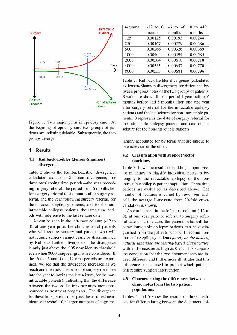
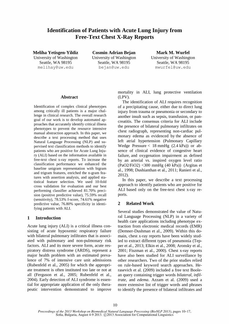
Figure 1: Two major paths in epilepsy care. Atthe begining of epilepsy care two groups of pa-tients are indistinguishable. Subsequently, the twogroups diverge.
4 Results
4.1 Kullback-Leibler (Jensen-Shannon)divergence
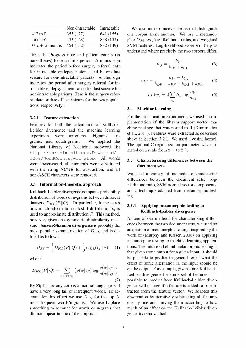
Table 2 shows the Kullback-Leibler divergence,calculated as Jensen-Shannon divergence, forthree overlapping time periods—the year preced-ing surgery referral, the period from 6 months be-fore surgery referral to six months after surgery re-ferral, and the year following surgery referral, forthe intractable epilepsy patients; and, for the non-intractable epilepsy patients, the same time peri-ods with reference to the last seizure date.
As can be seen in the left-most column (-12 to0), at one year prior, the clinic notes of patientswho will require surgery and patients who willnot require surgery cannot easily be discriminatedby Kullback-Leibler divergence—the divergenceis only just above the .005 near-identity thresholdeven when 8000 unique n-grams are considered. Ifthe -6 to +6 and 0 to +12 time periods are exam-ined, we see that the divergence increases as wereach and then pass the period of surgery (or moveinto the year following the last seizure, for the non-intractable patients), indicating that the differencebetween the two collections becomes more pro-nounced as treatment progresses. The divergencefor these time periods does pass the assumed near-identity threshold for larger numbers of n-grams,
n-grams -12 to 0months
-6 to +6months
0 to +12months
125 0.00125 0.00193 0.00244250 0.00167 0.00229 0.00286500 0.00266 0.00326 0.003891000 0.00404 0.00494 0.005852000 0.00504 0.00618 0.007184000 0.00535 0.00657 0.007708000 0.00555 0.00681 0.00796
Table 2: Kullback-Leibler divergence (calculatedas Jensen-Shannon divergence) for difference be-tween progress notes of the two groups of patients.Results are shown for the period 1 year before, 6months before and 6 months after, and one yearafter surgery referral for the intractable epilepsypatients and the last seizure for non-intractable pa-tients. 0 represents the date of surgery referral forthe intractable epilepsy patients and date of lastseizure for the non-intractable patients.
largely accounted for by terms that are unique toone notes set or the other.
4.2 Classification with support vectormachines
Table 3 shows the results of building support vec-tor machines to classify individual notes as be-longing to the intractable epilepsy or the non-intractable epilepsy patient population. Three timeperiods are evaluated, as described above. Thenumber of features is varied by row. For eachcell, the average F-measure from 20-fold cross-validation is shown.
As can be seen in the left-most column (-12 to0), at one year prior to referral to surgery refer-ral date or last seizure, the patients who will be-come intractable epilepsy patients can be distin-guished from the patients who will become non-intractable epilepsy patients purely on the basis ofnatural language processing-based classificationwith an F-measure as high as 0.95. This supportsthe conclusion that the two document sets are in-deed different, and furthermore illustrates that thisdifference can be used to predict which patientswill require surgical intervention.
4.3 Characterizing the differences betweenclinic notes from the two patientpopulations
Tables 4 and 5 show the results of three meth-ods for differentiating between the document col-
4
n-grams -12 to 0months
-6 to +6months
0 to +12months
125 0.8885 0.9217 0.9476250 0.8928 0.9297 0.9572500 0.9107 0.9367 0.96671000 0.9245 0.9496 0.96922000 0.9417 0.9595 0.97894000 0.9469 0.9661 0.98008000 0.9510 0.9681 0.9810
Table 3: Average F1 for the three time periodsdescribed above, with increasing numbers of fea-tures. Values are the average of 20-fold cross-validation. See Figure 2 for an explanation of thetime periods.
lections representing the two patient populations.The methodology for each is described above. Themost strongly distinguishing features when justthe 125 most frequent features are used are shownin Table 4, and the most strongly distinguishingfeatures when the 8,000 most frequent features areused are shown in Table 5. Impressionistically,two trends emerge. One is that more clearly clini-cally significant features are shown to have strongdiscriminatory power when the 8,000 most fre-quent features are used than when the 125 mostfrequent features are used. This result is sup-ported by the Kullback-Leibler divergence results,which demonstrated the most divergent vocabular-ies with larger numbers of n-grams. The othertrend is that the SVM classifier does a better jobof picking out clinically relevant features. Thishas implications for the design of clinical decisionsupport systems that utilize our approach.
5 Discussion
5.1 Behavior of Kullback-Leibler divergence
Kullback-Leibler divergence varies with the num-ber of words considered. When the vocabulariesof two document sets are merged and the wordsare ordered by overall frequency, the further downthe list we go, the higher the Kullback-Leiblerdivergence can be expected to be. This is be-cause the highest-frequency words in the com-bined set will generally be frequent in both sourcecorpora, and therefore carry similar probabilitymass. As we progress further down the list offrequency-ranked words, we include progressivelyless-common words, with diverse usage patterns,which are likely to reflect the differences between
the two document sets, if there are any. Thus, theKullback-Leibler divergence will rise.
To understand the intuition here, imagine look-ing at the Kullback-Leibler divergence when justthe 50 most-common words are considered. Thesewill be primarily function words, and their distri-butions are unlikely to differ much between thetwo document sets unless the syntax of the twocorpora is radically different. Beyond this set ofvery frequent common words will be words thatmay be relatively frequent in one set as comparedto the other, contributing to divergence betweenthe sets.
In Table 2, the observed behavior for our twodocument collections follows this expected pat-tern. However, the divergence between the vocab-ularies remains close to the assumed near-identitythreshold of 0.005, even when larger numbers ofn-grams are considered. The divergence never ex-ceeds 0.01; this level of divergence for larger num-bers of n-grams is consistent with prior analyses ofhighly similar corpora (Verspoor et al., 2009).
We attribute this similarity to two factors. Thefirst is that both document sets derive from a singledepartment within a single hospital; a relativelysmall number of doctors are responsible for au-thoring the notes and there may exist specific hos-pital protocols related to their content. The secondis that the clinical contexts from which our twodocument sets are derived are highly related, inthat all the patients are epilepsy patients. While wehave demonstrated that there are clear differencesbetween the two sets, it is also to be expected thatthey would have many words in common. Thenature of clinical notes combined with the shareddisease context results in generally consistent vo-cabulary and hence low overall divergence.
5.2 Behavior of classifier
Table 3 demonstrates that classifier performanceincreases as the number of features increases. Thisindicates that as more terms are considered, thebasis for differentiating between the two differentdocument collections is stronger.
Examining the SVM normal vector components(SVMW) in Tables 4 and 5, we find that unigrams,bigrams and trigrams are useful in differentiationbetween the two patient populations. While noquadrigrams appear in this table, they may in factcontribute to classifier performance. We will per-form an ablation study in future work to quantify
5
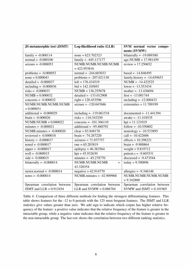
JS metamorphic test (JSMT) Log-likelihood ratio (LLR) SVM normal vector compo-nents (SVMW)
family = -0.000114 none = 623.702323 bilaterally = -19.009380normal = -0.000106 family = -445.117177 age.NUMB = 17.981459seizure = -0.000053 NUMB.NUMB.NUMB.NUMB
= 422.953816review = 17.250652
problems = -0.000053 normal = -244.603033 based = -14.846495none = 0.000043 problems = -207.021130 family.history = -14.659653detailed = -0.000037 left = 176.434519 NUMB = -14.422525including = -0.000036 bid = 142.105691 lower = -13.553434risks = -0.000033 NUMB = 136.255678 mother = -13.436694NUMB = 0.000032 detailed = -133.012908 first = -13.001744concerns = -0.000032 right = 120.453596 including = -12.800433NUMB.NUMB.NUMB.NUMB= 0.000031
seizure = -120.047686 extremities = 11.709199
additional = -0.000029 including = -119.061518 documented = -11.441394brain = -0.000026 risks = -116.543250 awake = -11.418535NUMB.NUMB = 0.000022 concerns = -101.366110 hpi = 11.121019minutes = -0.000021 additional = -95.880792 follow = -10.550802NUMB.minutes = -0.000020 clear = 83.848170 neurology = -10.533895reviewed = -0.000018 brain = -74.267220 call = -10.422606history = -0.000017 seizures = 71.937757 effects = 10.298221noted = -0.000017 one = 65.203819 brain = -9.900864upper = -0.000017 epilepsy = 46.383564 weight = 9.819712well = -0.000015 hpi = 45.932630 patient.s = -9.603531side = -0.000015 minutes = -45.278770 discussed = -9.473544bilaterally = -0.000014 NUMB.NUMB.NUMB =
43.320354today = 9.390896
motor.normal = -0.000014 negative = 42.914770 allergies = -9.346146notes = -0.000014 NUMB.minutes = -42.909968 NUMB.NUMB.NUMB.NUMB
= 9.342800Spearman correlation betweenJSMT and LLR = 0.912454
Spearman correlation betweenLLR and SVMW = 0.086784
Spearman correlation betweenSVMW and JSMT = 0.101965
Table 4: Comparison of three different methods for finding the strongest differentiating features. Thistable shows features for the -12 to 0 periods with the 125 most frequent features. The JSMT and LLRstatistics give values greater than zero. We add sign to indicate which corpus has higher relative fre-quency of the feature: a positive value indicates that the relative frequency of the feature is greater in theintractable group, while a negative value indicates that the relative frequency of the feature is greater inthe non-intractable group. The last row shows the correlation between two different ranking statistics.
6
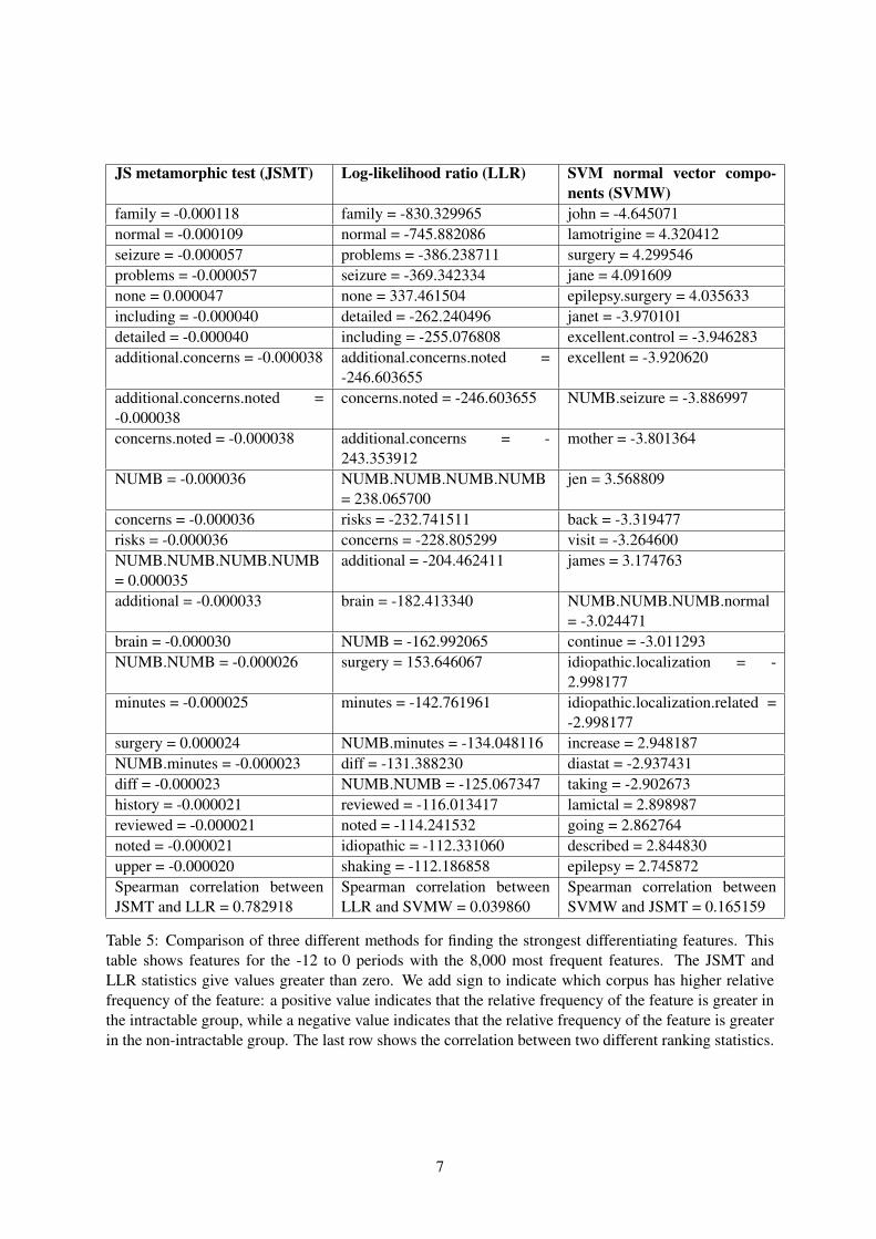
JS metamorphic test (JSMT) Log-likelihood ratio (LLR) SVM normal vector compo-nents (SVMW)
family = -0.000118 family = -830.329965 john = -4.645071normal = -0.000109 normal = -745.882086 lamotrigine = 4.320412seizure = -0.000057 problems = -386.238711 surgery = 4.299546problems = -0.000057 seizure = -369.342334 jane = 4.091609none = 0.000047 none = 337.461504 epilepsy.surgery = 4.035633including = -0.000040 detailed = -262.240496 janet = -3.970101detailed = -0.000040 including = -255.076808 excellent.control = -3.946283additional.concerns = -0.000038 additional.concerns.noted =
-246.603655excellent = -3.920620
additional.concerns.noted =-0.000038
concerns.noted = -246.603655 NUMB.seizure = -3.886997
concerns.noted = -0.000038 additional.concerns = -243.353912
mother = -3.801364
NUMB = -0.000036 NUMB.NUMB.NUMB.NUMB= 238.065700
jen = 3.568809
concerns = -0.000036 risks = -232.741511 back = -3.319477risks = -0.000036 concerns = -228.805299 visit = -3.264600NUMB.NUMB.NUMB.NUMB= 0.000035
additional = -204.462411 james = 3.174763
additional = -0.000033 brain = -182.413340 NUMB.NUMB.NUMB.normal= -3.024471
brain = -0.000030 NUMB = -162.992065 continue = -3.011293NUMB.NUMB = -0.000026 surgery = 153.646067 idiopathic.localization = -
2.998177minutes = -0.000025 minutes = -142.761961 idiopathic.localization.related =
-2.998177surgery = 0.000024 NUMB.minutes = -134.048116 increase = 2.948187NUMB.minutes = -0.000023 diff = -131.388230 diastat = -2.937431diff = -0.000023 NUMB.NUMB = -125.067347 taking = -2.902673history = -0.000021 reviewed = -116.013417 lamictal = 2.898987reviewed = -0.000021 noted = -114.241532 going = 2.862764noted = -0.000021 idiopathic = -112.331060 described = 2.844830upper = -0.000020 shaking = -112.186858 epilepsy = 2.745872Spearman correlation betweenJSMT and LLR = 0.782918
Spearman correlation betweenLLR and SVMW = 0.039860
Spearman correlation betweenSVMW and JSMT = 0.165159
Table 5: Comparison of three different methods for finding the strongest differentiating features. Thistable shows features for the -12 to 0 periods with the 8,000 most frequent features. The JSMT andLLR statistics give values greater than zero. We add sign to indicate which corpus has higher relativefrequency of the feature: a positive value indicates that the relative frequency of the feature is greater inthe intractable group, while a negative value indicates that the relative frequency of the feature is greaterin the non-intractable group. The last row shows the correlation between two different ranking statistics.
7
the contribution of the different feature sets. In ad-dition, we find that table 5 shows many clinicallyrelevant terms, such as seizure frequency (“ex-cellent [seizure] control“), epilepsy type (“local-ization related [epilepsy]”), etiology classification(“idiopathic [epilepsy]”), and drug names (“lamot-rigine”, “diastat”, “lamictal”), giving nearly com-plete history of the present illness.
6 Conclusion
The classification results from our machine learn-ing experiments support rejection of the null hy-pothesis of no detectable differences between theclinic notes of patients who will progress to thediagnosis of intractable epilepsy and patients whodo not progress to the diagnosis of intractableepilepsy. The results show that we can predictfrom an early stage of treatment which patientswill fall into these two classes based only on tex-tual data from the neurology clinic notes. As intu-ition would suggest, we find that the notes becomemore divergent and the ability to predict outcomeimproves as time progresses, but the most impor-tant point is that the outcome can be predictedfrom the earliest time period.
SVM classification demonstrates a stronger re-sult than the information-theoretic measures, usesless data, and needs just a single run. However, itis important to note that we cannot entirely relyon the argument from classification as the solemethodology in testing whether or not two doc-ument sets are similar or different. If the find-ing is positive, i.e., it is possible to train a classi-fier to distinguish between documents drawn fromthe two document sets, then interpreting the re-sults is straightforward. However, if documentsdrawn from the two document sets are not foundto be distinguishable by a classifier, one mustconsider the possibility of multiple possible con-founds, such as selection of an inappropriate clas-sification algorithm, extraction of the wrong fea-tures, bugs in the feature extraction software, etc.Having established that the two sets of clinicalnotes differ, we noted some identifying features ofclinic notes from the two populations, particularlywhen more terms were considered.
The Institute of Medicine explains that “. . . toaccommodate the reality that although profes-sional judgment will always be vital to shapingcare, the amount of information required for anygiven decision is moving beyond unassisted hu-
man capacity (Olsen et al., 2007).” This is surelythe case for those who care for the epileptic pa-tient. Technology like natural language processingwill ultimately serve as a basis for stable clinicaldecision support tools. It, however, is not a deci-sion making tool. Decision making is the respon-sibility of professional judgement. That judge-ment will labor over such questions as: what isthe efficacy of neurosurgery, what will be the longterm outcome, will there be any lasting damage,are we sure that all the medications have beentested, and how the family will adjust to a pooroutcome. In the end, it is that judgement that willdecide what is best; that decision will be supportedby research like what is presented here.
7 Acknowledgements
This work was supported in part by the NationalInstitutes of Health, Grants #1R01LM011124-01,and 1R01NS045911-01; the Cincinnati Chil-dren’s Hospital Medical Center’s: Research Foun-dation, Department of Pediatric Surgery and theDepartment of Paediatrics’s divisions of Neurol-ogy and Biomedical Informatics. We also wishto acknowledge the clinical and surgical wisdomprovided by Drs. John J. Hutton & Hansel M.Greiner, MD. K. Bretonnel Cohen was supportedby grants XXX YYY ZZZ. Karin Verspoor wassupported by NICTA, which is funded by the Aus-tralian Government as represented by the Depart-ment of Broadband, Communications and the Dig-ital Economy and the Australian Research Coun-cil.
References[Abhyankar et al.2012] Swapna Abhyankar, Kira Leis-
hear, Fiona M. Callaghan, Dina Demner-Fushman,and Clement J. McDonald. 2012. Lower short- andlong-term mortality associated with overweight andobesity in a large cohort study of adult intensive careunit patients. Critical Care, 16.
[Begley et al.2000] Charles E Begley, Melissa Famu-lari, John F Annegers, David R Lairson, Thomas FReynolds, Sharon Coan, Stephanie Dubinsky,Michael E Newmark, Cynthia Leibson, EL So, et al.2000. The cost of epilepsy in the united states: Anestimate from population-based clinical and surveydata. Epilepsia, 41(3):342–351.
[Dimitriadou et al.2011] Evgenia Dimitriadou, KurtHornik, Friedrich Leisch, David Meyer, and An-dreas Weingessel, 2011. e1071: Misc Func-tions of the Department of Statistics (e1071), TU
8
Wien. http://CRAN.R-project.org/package=e1071.R package version 1.5.
[Epilepsy Foundation2012] Epilepsy Foundation,2012. What is Epilepsy: Incidence and Prevalence.http://www.epilepsyfoundation.org/ aboutepilepsy/whatisepilepsy/ statistics.cfm.
[Himes et al.2009] Blanca E. Himes, Yi Dai, Isaac S.Kohane, Scott T. Weiss, and Marco F. Ramoni.2009. Prediction of chronic obstructive pulmonarydisease (copd) in asthma patients using electronicmedical records. Journal of the American MedicalInformatics Association, 16(3):371–379.
[Huang et al.under review] Sandy H. Huang, Paea LeP-endu, Srinivasan V Iyer, Anna Bauer-Mehren, CliffOlson, and Nigam H. Shah. under review. Develop-ing computational models for predicting diagnosesof depression. In American Medical Informatics As-sociation.
[Jonquet et al.2009] Clement Jonquet, Nigam H. Shah,Cherie H. Youn, Mark A. Musen, Chris Callendar,and Margaret-Anne Storey. 2009. NCBO Annota-tor: Semantic annotation of biomedical data. In 8thInternational Semantic Web Conference.
[Kwan and Brodie2000] Patrick Kwan and Martin JBrodie. 2000. Early identification of refrac-tory epilepsy. New England Journal of Medicine,342(5):314–319.
[Kwan et al.2010] Patrick Kwan, Alexis Arzimanoglou,Anne T Berg, Martin J Brodie, W Allen Hauser,Gary Mathern, Solomon L Moshe, Emilio Perucca,Samuel Wiebe, and Jacqueline French. 2010. Defi-nition of drug resistant epilepsy: consensus proposalby the ad hoc task force of the ilae commission ontherapeutic strategies. Epilepsia, 51(6):1069–1077.
[Manning and Schuetze1999] Christopher Manningand Hinrich Schuetze. 1999. Foundations ofstatistical natural language processing. MIT Press.
[Murphy and Kaiser2008] Christian Murphy and GailKaiser. 2008. Improving the dependability of ma-chine learning applications.
[Olsen et al.2007] LeighAnne Olsen, Dara Aisner, andJ Michael McGinnis. 2007. The learning healthcaresystem.
[Verspoor et al.2009] K. Verspoor, K.B. Cohen, andL. Hunter. 2009. The textual characteristics of tradi-tional and open access scientific journals are similar.BMC Bioinformatics, 10(1):183.
9
Proceedings of the 2013 Workshop on Biomedical Natural Language Processing (BioNLP 2013), pages 10–17,Sofia, Bulgaria, August 4-9 2013. c©2013 Association for Computational Linguistics
Identification of Patients with Acute Lung Injury from
Free-Text Chest X-Ray Reports
Meliha Yetisgen-Yildiz University of Washington
Seattle, WA 98195 [email protected]
Cosmin Adrian Bejan University of Washington
Seattle, WA 98195 [email protected]
Mark M. Wurfel University of Washington
Seattle, WA 98195 [email protected]
Abstract
Identification of complex clinical phenotypes
among critically ill patients is a major chal-
lenge in clinical research. The overall research
goal of our work is to develop automated ap-
proaches that accurately identify critical illness
phenotypes to prevent the resource intensive
manual abstraction approach. In this paper, we
describe a text processing method that uses
Natural Language Processing (NLP) and su-
pervised text classification methods to identify
patients who are positive for Acute Lung Inju-
ry (ALI) based on the information available in
free-text chest x-ray reports. To increase the
classification performance we enhanced the
baseline unigram representation with bigram
and trigram features, enriched the n-gram fea-
tures with assertion analysis, and applied sta-
tistical feature selection. We used 10-fold
cross validation for evaluation and our best
performing classifier achieved 81.70% preci-
sion (positive predictive value), 75.59% recall
(sensitivity), 78.53% f-score, 74.61% negative
predictive value, 76.80% specificity in identi-
fying patients with ALI.
1 Introduction
Acute lung injury (ALI) is a critical illness con-
sisting of acute hypoxemic respiratory failure
with bilateral pulmonary infiltrates that is associ-
ated with pulmonary and non-pulmonary risk
factors. ALI and its more severe form, acute res-
piratory distress syndrome (ARDS), represent a
major health problem with an estimated preva-
lence of 7% of intensive care unit admissions
(Rubenfeld et al., 2005) for which the appropri-
ate treatment is often instituted too late or not at
all (Ferguson et al., 2005; Rubenfeld et al.,
2004). Early detection of ALI syndrome is essen-
tial for appropriate application of the only thera-
peutic intervention demonstrated to improve
mortality in ALI, lung protective ventilation
(LPV).
The identification of ALI requires recognition
of a precipitating cause, either due to direct lung
injury from trauma or pneumonia or secondary to
another insult such as sepsis, transfusion, or pan-
creatitis. The consensus criteria for ALI include
the presence of bilateral pulmonary infiltrates on
chest radiograph, representing non-cardiac pul-
monary edema as evidenced by the absence of
left atrial hypertension (Pulmonary Capillary
Wedge Pressure < 18 mmHg (2.4 kPa)) or ab-
sence of clinical evidence of congestive heart
failure, and oxygenation impairment as defined
by an arterial vs. inspired oxygen level ratio
(PaO2/FiO2) <300 mmHg (40 kPa)) (Argitas et
al., 1998; Dushianthan et al., 2011; Ranieri et al.,
2012).
In this paper, we describe a text processing
approach to identify patients who are positive for
ALI based only on the free-text chest x-ray re-
ports.
2 Related Work
Several studies demonstrated the value of Natu-
ral Language Processing (NLP) in a variety of
health care applications including phenotype ex-
traction from electronic medical records (EMR)
(Demner-Dushman et al., 2009). Within this do-
main, chest x-ray reports have been widely stud-
ied to extract different types of pneumonia (Tep-
per et al., 2013; Elkin et al., 2008; Aronsky et al.,
2001; Fiszman et al., 2000). Chest x-ray reports
have also been studied for ALI surveillance by
other researchers. Two of the prior studies relied
on rule-based keyword search approaches. He-
rasevich et al. (2009) included a free text Boole-
an query containing trigger words bilateral, infil-
trate, and edema. Azzam et al. (2009) used a
more extensive list of trigger words and phrases
to identify the presence of bilateral infiltrates and
10
ALI. In another study, Solti et al. (2009) repre-
sented the content of chest x-ray reports using
character n-grams and applied supervised classi-
fication to identify chest x-ray reports consistent
with ALI. In our work, different from prior re-
search, we proposed a fully statistical approach
where (1) the content of chest x-ray reports was
represented by token n-grams, (2) statistical fea-
ture selection was applied to select the most in-
formative features, and (3) assertion analysis was
used to enrich the n-gram features. We also im-
plemented Azzam et al.’s approach based on the
information available in their paper and used it as
a baseline to compare performance results of our
approach to theirs.
3 Methods
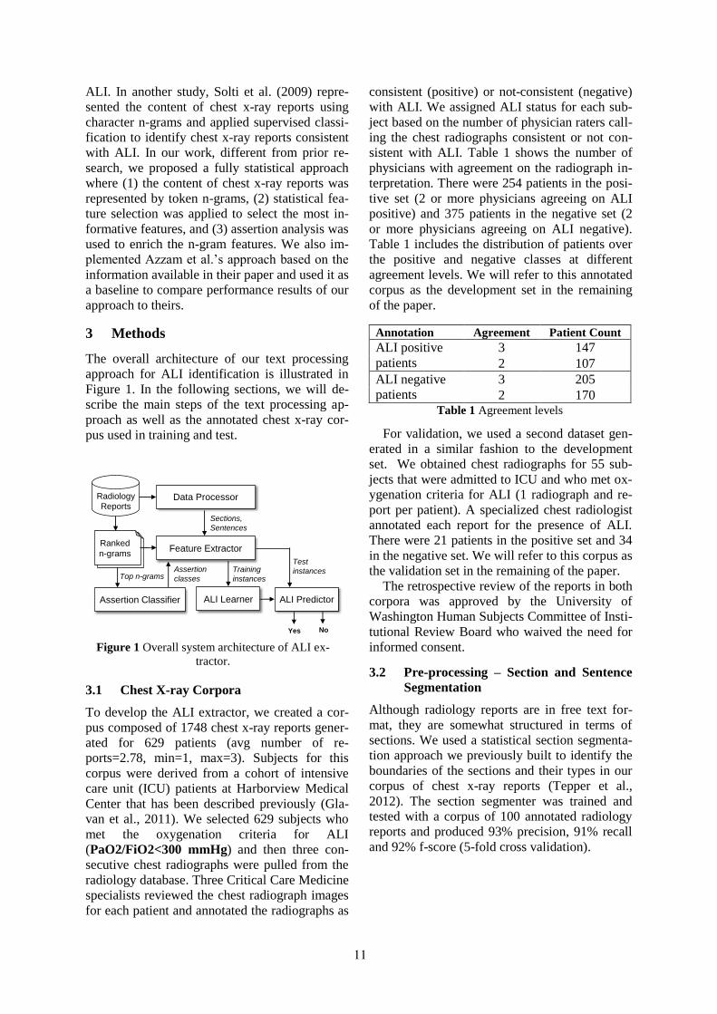
The overall architecture of our text processing
approach for ALI identification is illustrated in
Figure 1. In the following sections, we will de-
scribe the main steps of the text processing ap-
proach as well as the annotated chest x-ray cor-
pus used in training and test.
3.1 Chest X-ray Corpora
To develop the ALI extractor, we created a cor-
pus composed of 1748 chest x-ray reports gener-
ated for 629 patients (avg number of re-
ports=2.78, min=1, max=3). Subjects for this
corpus were derived from a cohort of intensive
care unit (ICU) patients at Harborview Medical
Center that has been described previously (Gla-
van et al., 2011). We selected 629 subjects who
met the oxygenation criteria for ALI
(PaO2/FiO2<300 mmHg) and then three con-
secutive chest radiographs were pulled from the
radiology database. Three Critical Care Medicine
specialists reviewed the chest radiograph images
for each patient and annotated the radiographs as
consistent (positive) or not-consistent (negative)
with ALI. We assigned ALI status for each sub-
ject based on the number of physician raters call-
ing the chest radiographs consistent or not con-
sistent with ALI. Table 1 shows the number of
physicians with agreement on the radiograph in-
terpretation. There were 254 patients in the posi-
tive set (2 or more physicians agreeing on ALI
positive) and 375 patients in the negative set (2
or more physicians agreeing on ALI negative).
Table 1 includes the distribution of patients over
the positive and negative classes at different
agreement levels. We will refer to this annotated
corpus as the development set in the remaining
of the paper.
For validation, we used a second dataset gen-
erated in a similar fashion to the development
set. We obtained chest radiographs for 55 sub-
jects that were admitted to ICU and who met ox-
ygenation criteria for ALI (1 radiograph and re-
port per patient). A specialized chest radiologist
annotated each report for the presence of ALI.
There were 21 patients in the positive set and 34
in the negative set. We will refer to this corpus as
the validation set in the remaining of the paper.
The retrospective review of the reports in both
corpora was approved by the University of
Washington Human Subjects Committee of Insti-
tutional Review Board who waived the need for
informed consent.
3.2 Pre-processing – Section and Sentence
Segmentation
Although radiology reports are in free text for-
mat, they are somewhat structured in terms of
sections. We used a statistical section segmenta-
tion approach we previously built to identify the
boundaries of the sections and their types in our
corpus of chest x-ray reports (Tepper et al.,
2012). The section segmenter was trained and
tested with a corpus of 100 annotated radiology
reports and produced 93% precision, 91% recall
and 92% f-score (5-fold cross validation).
Radiology
ReportsData Processor
Sections,
Sentences
Ranked
n-grams
ALI Learner ALI Predictor
Training
instances
Test
instances
Yes No
Assertion Classifier
Feature Extractor
Assertion
classesTop n-grams
Figure 1 Overall system architecture of ALI ex-
tractor.
Annotation Agreement Patient Count
ALI positive
patients
3 147
2 107
ALI negative
patients
3 205
2 170 Table 1 Agreement levels
11
After identifying the report sections, we used the
OpenNLP1
sentence chunker to identify the
boundaries of sentences in the section bodies.
This pre-processing step identified 8,659 sec-
tions and 15,890 sentences in 1,748 reports of the
development set and 206 sections and 414 sen-
tences in 55 reports of the validation set. We
used the section information to filter out the sec-
tions with clinician signatures (e.g., Interpreted
By, Contributing Physicians, Signed By). We
used the sentences to extract the assertion values
associated with n-gram features as will be ex-
plained in a later section.
3.3 Feature Selection
Representing the information available in the
free-text chest x-ray reports as features is critical
in identifying patients with ALI. In our represen-
tation, we created one feature vector for each
patient. We used unigrams as the baseline repre-
sentation. In addition, we used bigrams and tri-
grams as features. We observed that the chest x-
ray reports in our corpus are short and not rich in
terms of medical vocabulary usage. Based on this
observation, we decided not to include any medi-
cal knowledge-based features such as UMLS
concepts or semantic types. Table 2 summarizes
the number of distinct features for each feature
type used to represent the 1,748 radiology reports
for 629 patients.
As can be seen from the table, for bigrams and
trigrams, the feature set sizes is quite high. Fea-
ture selection algorithms have been successfully
applied in text classification in order to improve
the classification accuracy (Wenqian et al.,
2007). In previous work, we applied statistical
feature selection to the problem of pneumonia
detection from ICU reports (Bejan et al., 2012).
By significantly reducing the dimensionality of
the feature space, they improved the efficiency of
the pneumonia classifiers and provided a better
understanding of the data.
We used statistical hypothesis testing to de-
termine whether there is an association between
a given feature and the two categories of our
problem (i.e, positive and negative ALI). Specif-
ically, we computed the χ2
statistics (Manning
1 OpenNLP. Available at: http://opennlp.apache.org/
and Schutze, 1999) which generated an ordering
of features in the training set. We used 10-fold
cross validation (development set) in our overall
performance evaluation. Table 3 lists the top 15
unigrams, bigrams, and trigrams ranked by χ2
statistics in one of ten training sets we used in
evaluation. As can be observed from the table,
many of the features are closely linked to ALI.
Once the features were ranked and their corre-
sponding threshold values (N) were established,
we built a feature vector for each patient. Specif-
ically, given the subset of N relevant features
extracted from the ranked list of features, we
considered in the representation of a given pa-
tient’s feature vector only the features from the
subset of relevant features that were also found
in the chest x-ray reports of the patient. There-
fore, the size of the feature space is equal to the
size of relevant features subset (N) whereas the
length of each feature vector will be at most this
value.
3.4 Assertion Analysis
We extended our n-gram representation with as-
sertion analysis. We built an assertion classifier
(Bejan et al., 2013) based on the annotated cor-
pus of 2010 Integrating Biology and the Beside
(i2b2) / Veteran’s Affairs (VA) NLP challenge
(Uzuner et al., 2011). The 2010 i2b2/VA chal-
lenge introduced assertion classification as a
Unigram Bigram Trigram Diffuse diffuse lung opacities con-
sistent with
Atelectasis lung opacities diffuse lung opaci-
ties
Pulmonary pulmonary edema change in diffuse
Consistent consistent with lung opacities
consistent
Edema opacities consistent in diffuse lung
Alveolar in diffuse with pulmonary
edema
Opacities diffuse bilateral consistent with
pulmonary
Damage with pulmonary low lung volumes
Worsening alveolar damage or alveolar damage
Disease edema or pulmonary edema
pneumonia
Bilateral low lung diffuse lung dis-
ease
Clear edema pneumonia edema pneumonia
no
Severe or alveolar diffuse bilateral
opacities
Injury lung disease lungs are clear
Bibasilar pulmonary opacities lung volumes with
Table 3 Top 15 most informative unigrams, bigrams,
and trigrams for ALI classification according to χ2
statistics. Feature Type # of Distinct Features
Unigram (baseline) 1,926
Bigram 10,190
Trigram 17,798
Table 2 Feature set sizes of the development set.
12
shared task, formulated such that each medical
concept mentioned in a clinical report (e.g.,
asthma) is associated with a specific assertion
category (present, absent, conditional, hypothet-
ical, possible, and not associated with the pa-
tient). We defined a set of novel features that
uses the syntactic information encoded in de-
pendency trees in relation to special cue words
for these categories. We also defined features to
capture the semantics of the assertion keywords
found in the corpus and trained an SVM multi-
class classifier with default parameter settings.
Our assertion classifier outperformed the state-
of-the-art results and achieved 79.96% macro-
averaged F-measure and 94.23% micro-averaged
F-measure on the i2b2/VA challenge test data.
For each n-gram feature (e.g., pneumonia), we
used the assertion classifier to determine whether
it is present or absent based on contextual infor-
mation available in the sentence the feature ap-
peared in (e.g., Feature: pneumonia, Sentence:
There is no evidence of pneumonia, congestive
heart failure, or other acute process., Assertion:
absent). We added the identified assertion value
to the feature (e.g., pneumonia_absent). The fre-
quencies of each assertion type in our corpus are
presented in Table 4. Because chest x-rays do not
include family history, there were no instances of
not associated with the patient. We treated the
three assertion categories that express hedging
(conditional, hypothetical, possible) as the pre-
sent category.
3.5 Classification
For our task of classifying ALI patients, we
picked the Maximum Entropy (MaxEnt) algo-
rithm due to its good performance in text classi-
fication tasks (Berger et al., 1996). In our exper-
iments, we used the MaxEnt implementation in a
machine learning package called Mallet2.
4 Results
4.1 Metrics
We evaluated the performance by using precision
(positive predictive value), recall (sensitivity),
negative predictive value, specificity, f-score,
and accuracy. We used 10-fold cross validation
to measure the performance of our classifiers on
the development set. We evaluated the best per-
forming classifier on the validation set.
4.2 Experiments with Development Set
We designed three groups of experiments to ex-
plore the effects of (1) different n-gram features,
(2) feature selection, (3) assertion analysis of
features on the classification of ALI patients. We
defined two baselines to compare the perfor-
mance of our approaches. In the first baseline,
we implemented the Azzam et. al.’s rule-based
approach (2009). In the second baseline, we only
represented the content of chest x-ray reports
with unigrams.
4.3 N-gram Experiments
Table 5 summarizes the performance of n-gram
features. When compared to the baseline uni-
gram representation, gradually adding bigrams
(uni+bigram) and trigrams (uni+bi+trigram) to
the baseline increased the precision and specifici-
ty by 4%. Recall and NPV remained the same.
Azzam et. al.’s rule-based baseline generated
higher recall but lower precision when compared
to n-gram features. The best f-score (64.45%)
was achieved with the uni+bi+trigram represen-
tation.
4.4 Feature Selection Experiments
To understand the effect of large feature space on
classification performance, we studied how the
performance of our system evolves for various
threshold values (N) on the different combina-
tions of χ2
ranked unigram, bigram, and trigram
features. Table 6 includes a subset of the results
we collected for different values of N. As listed
2 Mallet. Available at: http://mallet.cs.umass.edu
Assertion Class Frequency
Present 206,863
Absent 13,961
Conditional 4
Hypothetical 330
Possible 3,980
Table 4 Assertion class frequencies.
System configuration TP TN FP FN Precision/
PPV
Recall/
Sensitivity NPV Specificity F-Score Accuracy
Baseline#1–Azzam et. al. (2009) 201 184 191 53 51.27 79.13 77.64 49.07 62.23 61.21
Baseline#2–unigram 156 288 87 98 64.20 61.42 74.61 76.80 62.78 70.59
Uni+bigram 156 296 79 98 66.38 61.42 75.13 78.93 63.80 71.86
Uni+bi+trigram 155 303 72 99 68.28 61.02 75.37 80.80 64.45 72.81
Table 5 Performance evaluation on development set with no feature selection. TP: True positive, TN: True nega-
tive, FP: False positive, FN: False negative, PPV: Positive predictive value, NPV: Negative predictive value. The
row with the heighted F-Score is highlighted.
13
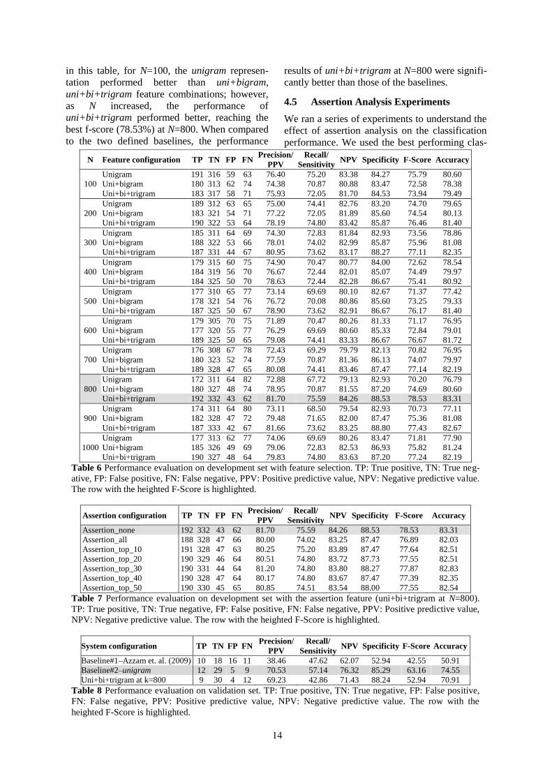
in this table, for N=100, the unigram represen-
tation performed better than uni+bigram,
uni+bi+trigram feature combinations; however,
as N increased, the performance of
uni+bi+trigram performed better, reaching the
best f-score (78.53%) at N=800. When compared
to the two defined baselines, the performance
results of uni+bi+trigram at N=800 were signifi-
cantly better than those of the baselines.
4.5 Assertion Analysis Experiments
We ran a series of experiments to understand the
effect of assertion analysis on the classification
performance. We used the best performing clas-
N Feature configuration TP TN FP FN Precision/
PPV
Recall/
Sensitivity NPV Specificity F-Score Accuracy
100
Unigram 191 316 59 63 76.40 75.20 83.38 84.27 75.79 80.60
Uni+bigram 180 313 62 74 74.38 70.87 80.88 83.47 72.58 78.38
Uni+bi+trigram 183 317 58 71 75.93 72.05 81.70 84.53 73.94 79.49
200
Unigram 189 312 63 65 75.00 74.41 82.76 83.20 74.70 79.65
Uni+bigram 183 321 54 71 77.22 72.05 81.89 85.60 74.54 80.13
Uni+bi+trigram 190 322 53 64 78.19 74.80 83.42 85.87 76.46 81.40
300
Unigram 185 311 64 69 74.30 72.83 81.84 82.93 73.56 78.86
Uni+bigram 188 322 53 66 78.01 74.02 82.99 85.87 75.96 81.08
Uni+bi+trigram 187 331 44 67 80.95 73.62 83.17 88.27 77.11 82.35
400
Unigram 179 315 60 75 74.90 70.47 80.77 84.00 72.62 78.54
Uni+bigram 184 319 56 70 76.67 72.44 82.01 85.07 74.49 79.97
Uni+bi+trigram 184 325 50 70 78.63 72.44 82.28 86.67 75.41 80.92
500
Unigram 177 310 65 77 73.14 69.69 80.10 82.67 71.37 77.42
Uni+bigram 178 321 54 76 76.72 70.08 80.86 85.60 73.25 79.33
Uni+bi+trigram 187 325 50 67 78.90 73.62 82.91 86.67 76.17 81.40
600
Unigram 179 305 70 75 71.89 70.47 80.26 81.33 71.17 76.95
Uni+bigram 177 320 55 77 76.29 69.69 80.60 85.33 72.84 79.01
Uni+bi+trigram 189 325 50 65 79.08 74.41 83.33 86.67 76.67 81.72
700
Unigram 176 308 67 78 72.43 69.29 79.79 82.13 70.82 76.95
Uni+bigram 180 323 52 74 77.59 70.87 81.36 86.13 74.07 79.97
Uni+bi+trigram 189 328 47 65 80.08 74.41 83.46 87.47 77.14 82.19
800
Unigram 172 311 64 82 72.88 67.72 79.13 82.93 70.20 76.79
Uni+bigram 180 327 48 74 78.95 70.87 81.55 87.20 74.69 80.60
Uni+bi+trigram 192 332 43 62 81.70 75.59 84.26 88.53 78.53 83.31
900
Unigram 174 311 64 80 73.11 68.50 79.54 82.93 70.73 77.11
Uni+bigram 182 328 47 72 79.48 71.65 82.00 87.47 75.36 81.08
Uni+bi+trigram 187 333 42 67 81.66 73.62 83.25 88.80 77.43 82.67
1000
Unigram 177 313 62 77 74.06 69.69 80.26 83.47 71.81 77.90
Uni+bigram 185 326 49 69 79.06 72.83 82.53 86.93 75.82 81.24
Uni+bi+trigram 190 327 48 64 79.83 74.80 83.63 87.20 77.24 82.19
Table 6 Performance evaluation on development set with feature selection. TP: True positive, TN: True neg-
ative, FP: False positive, FN: False negative, PPV: Positive predictive value, NPV: Negative predictive value.
The row with the heighted F-Score is highlighted.
Assertion configuration TP TN FP FN Precision/
PPV
Recall/
Sensitivity NPV Specificity F-Score Accuracy
Assertion_none 192 332 43 62 81.70 75.59 84.26 88.53 78.53 83.31
Assertion_all 188 328 47 66 80.00 74.02 83.25 87.47 76.89 82.03
Assertion_top_10 191 328 47 63 80.25 75.20 83.89 87.47 77.64 82.51
Assertion_top_20 190 329 46 64 80.51 74.80 83.72 87.73 77.55 82.51
Assertion_top_30 190 331 44 64 81.20 74.80 83.80 88.27 77.87 82.83
Assertion_top_40 190 328 47 64 80.17 74.80 83.67 87.47 77.39 82.35
Assertion_top_50 190 330 45 65 80.85 74.51 83.54 88.00 77.55 82.54
Table 7 Performance evaluation on development set with the assertion feature (uni+bi+trigram at N=800).
TP: True positive, TN: True negative, FP: False positive, FN: False negative, PPV: Positive predictive value,
NPV: Negative predictive value. The row with the heighted F-Score is highlighted.
System configuration TP TN FP FN Precision/
PPV
Recall/
Sensitivity NPV Specificity F-Score Accuracy
Baseline#1–Azzam et. al. (2009) 10 18 16 11 38.46 47.62 62.07 52.94 42.55 50.91
Baseline#2–unigram 12 29 5 9 70.53 57.14 76.32 85.29 63.16 74.55
Uni+bi+trigram at k=800 9 30 4 12 69.23 42.86 71.43 88.24 52.94 70.91
Table 8 Performance evaluation on validation set. TP: True positive, TN: True negative, FP: False positive,
FN: False negative, PPV: Positive predictive value, NPV: Negative predictive value. The row with the
heighted F-Score is highlighted.
14
sifier with uni+bi+trigram at N=800 in our ex-
periments. We applied assertion analysis to all
800 features as well as only a small set of top
ranked 10×k (1≤k≤5) features which were ob-
served to be closely related to ALI (e.g., diffuse,
opacities, pulmonary edema). We hypothesized
applying assertion analysis would inform the
classifier on the presence and absence of those
terms which would potentially decrease the false
positive and negative counts.
Table 7 summarizes the results of our experi-
ments. When we applied assertion analysis to all
800 features, the performance slightly dropped
when compared to the performance with no as-
sertion analysis. When assertion analysis applied
to only top ranked features, the best f-score per-
formance was achieved with assertion analysis
with top 30 features; however, it was still slightly
lower than the f-score with no assertion analysis.
The differences are not statistically significant.
4.6 Experiments with Validation Set
We used the validation set to explore the general-
izability of the proposed approach. To accom-
plish this we run the best performing classifier
(uni+bi+trigram at N=800) and two defined
baselines on the validation set. We re-trained the
uni+bi+trigram at N=800 classifier and unigram
baseline on the complete development set.
Table 8 includes the performance results. The
second baseline with unigrams performed the
best and Azzam et. al.’s baseline performed the
worst in identifying the patients with ALI in the
validation set.
5 Discussion
Our best system achieved an f-score of 78.53
(precision=81.70, recall=75.59) on the develop-
ment set. While the result is encouraging and
significantly better than the f-score of a previous-
ly published system (f-score=62.23, preci-
sion=51.27, recall=79.13), there is still room for
improvement.
There are several important limitations to our
current development dataset. First, the annotators
who are pulmonary care specialists used only the
x-ray images to annotate the patients. However,
the classifiers were trained based on the features
extracted from the radiologists’ free-text inter-
pretation of the x-ray images. In one false posi-
tive case, the radiologist has written “Bilateral
diffuse opacities, consistent with pulmonary
edema. Bibasilar atelectasis.” in the chest x-ray
report, however all three pulmonary care special-
ists annotated the case as negative based on their
interpretation of images. Because the report con-
sisted of many very strong features indicative of
ALI, our classifier falsely identified the patient
as positive with a very high prediction probabil-
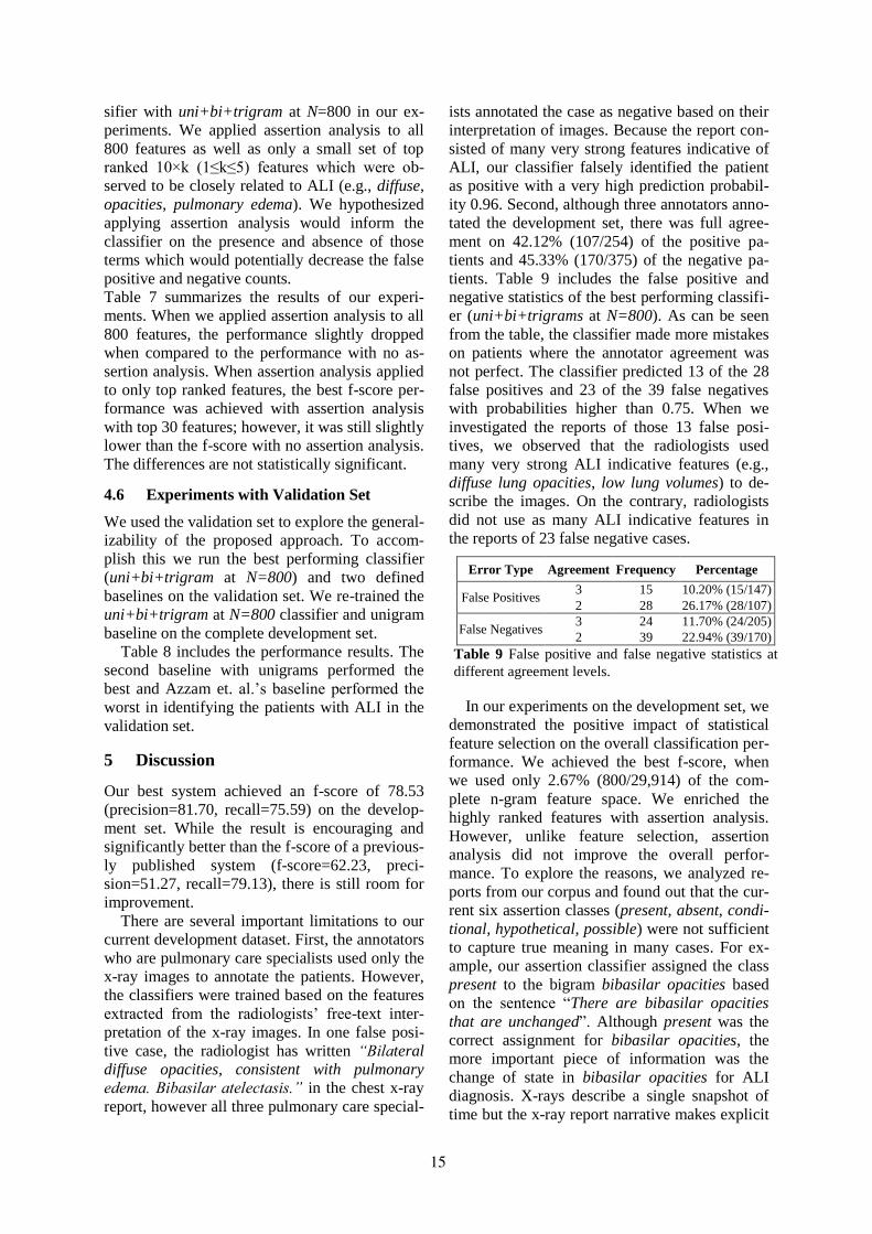
ity 0.96. Second, although three annotators anno-
tated the development set, there was full agree-
ment on 42.12% (107/254) of the positive pa-
tients and 45.33% (170/375) of the negative pa-
tients. Table 9 includes the false positive and
negative statistics of the best performing classifi-
er (uni+bi+trigrams at N=800). As can be seen
from the table, the classifier made more mistakes
on patients where the annotator agreement was
not perfect. The classifier predicted 13 of the 28
false positives and 23 of the 39 false negatives
with probabilities higher than 0.75. When we
investigated the reports of those 13 false posi-
tives, we observed that the radiologists used
many very strong ALI indicative features (e.g.,
diffuse lung opacities, low lung volumes) to de-
scribe the images. On the contrary, radiologists
did not use as many ALI indicative features in
the reports of 23 false negative cases.
In our experiments on the development set, we
demonstrated the positive impact of statistical
feature selection on the overall classification per-
formance. We achieved the best f-score, when
we used only 2.67% (800/29,914) of the com-
plete n-gram feature space. We enriched the
highly ranked features with assertion analysis.
However, unlike feature selection, assertion
analysis did not improve the overall perfor-
mance. To explore the reasons, we analyzed re-
ports from our corpus and found out that the cur-
rent six assertion classes (present, absent, condi-
tional, hypothetical, possible) were not sufficient
to capture true meaning in many cases. For ex-
ample, our assertion classifier assigned the class
present to the bigram bibasilar opacities based
on the sentence “There are bibasilar opacities
that are unchanged”. Although present was the
correct assignment for bibasilar opacities, the
more important piece of information was the
change of state in bibasilar opacities for ALI
diagnosis. X-rays describe a single snapshot of
time but the x-ray report narrative makes explicit
Error Type Agreement Frequency Percentage
False Positives 3 15 10.20% (15/147)
2 28 26.17% (28/107)
False Negatives 3 24 11.70% (24/205)
2 39 22.94% (39/170)
Table 9 False positive and false negative statistics at
different agreement levels.
15
or, more often implicit references to a previous
x-ray. In this way, the sequence of x-ray reports
is used not only to assess a patient’s health at a
moment in time but also to monitor the change.
We recently defined a schema to annotate change
of state for clinical events in chest x-ray reports
(Vanderwende et al., 2013). We will use this an-
notation schema to create an annotated corpus
for training models to enrich the assertion fea-
tures for ALI classification.
The results on the validation set revealed that
the classification performance degraded signifi-
cantly when training and test data do not come
from the same dataset. There are multiple rea-
sons to this effect. First, the two datasets had dif-
ferent language characteristics. Although both
development and validation sets included chest
x-ray reports, only 2,488 of the 3,305 (75.28%)
n-gram features extracted from the validation set
overlapped with the 29,914 n-gram features ex-
tracted from the development set. We suspect
that this is the main reason why our best per-
forming classifier with feature selection trained
on the development set did not perform as well
as the unigram baseline on the validation set.
Second, the validation set included only 55 pa-
tients and each patient had only one chest x-ray
report unlike the development set where each
patient had 2.78 reports on the average. In other
words, the classifiers trained on the development
set with richer content made poor predictions on
the validation set with more restricted content.
Third, because the number of patients in the val-
idation set was too small, each false positive and
negative case had a huge impact on the overall
performance.
6 Conclusion
In this paper, we described a text processing ap-
proach to identify patients with ALI from the
information available in their corresponding free-
text chest x-ray reports. To increase the classifi-
cation performance, we (1) enhanced the base-
line unigram representation with bigram and tri-
gram features, (2) enriched the n-gram features
with assertion analysis, and (3) applied statistical
feature selection. Our proposed methodology of
ranking all the features using statistical hypothe-
sis testing and selecting only the most relevant
ones for classification resulted in significantly
improving the performance of a previous system
for ALI identification. The best performing clas-
sifier achieved 81.70% precision (positive pre-
dictive value), 75.59% recall (sensitivity),
78.53% f-score, 74.61% negative predictive val-
ue, 76.80% specificity in identifying patients
with ALI when using the uni+bi+trigram repre-
sentation at N=800. Our experiments showed
that assertion values did not improve the overall
performance. For future work, we will work on
defining new semantic features that will enhance
the current assertion definition and capture the
change of important events in radiology reports.
Acknowledgements
The work is partly supported by the Institute of
Translational Health Sciences (UL1TR000423),
and Microsoft Research Connections. We would
also like to thank the anonymous reviewers for
helpful comments.
References
Aronsky D, Fiszman M, Chapman WW, Haug PJ.
Combining decision support methodologies to di-
agnose pneumonia. AMIA Annu Symp Proc.,
2001:12-16.
Artigas A, Bernard GR, Carlet J, Dreyfuss D, Gatti-
noni L, Hudson L, Lamy M, Marini JJ, Matthay
MA, Pinsky MR, Spragg R, Suter PM. The Ameri-
can-European Consensus Conference on ARDS,
part 2: Ventilatory, pharmacologic, supportive
therapy, study design strategies, and issues related
to recovery and remodeling. Acute respiratory dis-
tress syndrome. Am J Respir Crit Care Med.
1998;157(4 Pt1):1332-47.
Azzam HC, Khalsa SS, Urbani R, Shah CV, Christie
JD, Lanken PN, Fuchs BD. Validation study of an
automated electronic acute lung injury screening
tool. J Am Med Inform Assoc. 2009; 16(4):503-8.
Bejan CA, Xia F, Vanderwende L, Wurfel M, Yet-
isgen-Yildiz M. Pneumonia identification using
statistical feature selection. J Am Med Inform As-
soc. 2012; 19(5):817-23.
Bejan CA, Vanderwende L, Xia F, Yetisgen-Yildiz
M. Assertion Modeling and its role in clinical phe-
notype identification. J Biomed Inform. 2013;
46(1):68-74.
Berger AL, Pietra SAD, Pietra VJD. A maximum
entropy approach to natural language processing.
Journal of Computational Linguistics. 1996;
22(1):39-71.
Demner-Fushman D, Chapman WW, McDonald CJ.
What can natural language processing do for clini-
cal decision support? J Biomed Inform. 2009;
42(5):760-72.
Dushianthan A, Grocott MPW, Postle AD, Cusack R.
Acute respiratory distress syndrome and acute lung
injury. Postgrad Med J. 2011; 87:612-622.
16
Elkin PL, Froehling D, Wahner-Roedler D, Trusko B,
Welsh G, Ma H, Asatryan AX, Tokars JI, Rosen-
bloom ST, Brown SH. NLP-based identification of
pneumonia cases from free-text radiological re-
ports. AMIA Annu Symp Proc. 2008; 6:172-6.
Ferguson ND, Frutos-Vivar F, Esteban A, Fernández-
Segoviano P, Aramburu JA, Nájera L, Stewart TE.
Acute respiratory distress syndrome: underrecogni-
tion by clinicians and diagnostic accuracy of three
clinical definitions. Crit Care Med. 2005;
33(10):2228-34.
Fiszman M, Chapman WW, Aronsky D, Evans RS,
Haug PJ. Automatic detection of acute bacterial
pneumonia from chest X-ray reports. J Am Med In-
form Assoc. 2000;7(6):593-604.
Glavan BJ, Holden TD, Goss CH, Black RA, Neff
MJ, Nathens AB, Martin TR, Wurfel MM;
ARDSnet Investigators. Genetic variation in the
FAS gene and associations with acute lung injury.
Am J Respir Crit Care Med. 2011;183(3):356-63.
Herasevich V, Yilmaz M, Khan H, Hubmayr RD,
Gajic O. Validation of an electronic surveillance
system for acute lung injury. Intensive Care Med.
2009; 35(6):1018-23.
Manning CD, Schutze H. Foundations of statistical
natural language processing. MIT Press 1999.
Ranieri VM, Rubenfeld GD, Thompson BT, Ferguson
ND, Caldwell E, Fan E, Camporota L, Slutsky AS.
Acute Respiratory Distress Syndrome. The Berlin
Definition. JAMA. 2012; 307(23): 2526-2533.
Rubenfeld GD, Caldwell E, Peabody E, Weaver J,
Martin DP, Neff M, Stern EJ, Hudson LD. Inci-
dence and outcomes of acute lung injury. N Engl J
Med. 2005; 353(16):1685-93.
Rubenfeld GD, Cooper C, Carter G, Thompson BT,
Hudson LD. Barriers to providing lung-protective
ventilation to patients with acute lung injury. Crit
Care Med. 2004; 32(6):1289-93.
Solti I, Cooke CR, Xia F, Wurfel MM. Automated
Classification of Radiology Reports for Acute
Lung Injury: Comparison of Keyword and Ma-
chine Learning Based Natural Language Pro-
cessing Approaches. Proceedings (IEEE Int Conf
Bioinformatics Biomed). 2009;314-319.
Tepper M, Capurro D, Xia F, Vanderwende L, Yet-
isgen-Yildiz M. Statistical Section Segmentation in
Free-Text Clinical Records. Proceedings of the In-
ternational Conference on Language Resources and
Evaluation (LREC), Istanbul, May 2012.
Tepper M, Evans HL, Xia F, Yetisgen-Yildiz M.
Modeling Annotator Rationales with Application
to Pneumonia Classification. Proceedings of Ex-
panding the Boundaries of Health Informatics Us-
ing AI Workshop of AAAI'2013, Bellevue, WA;
2013.
Uzuner O, South BR, Shen S, DuVall SL. 2010
i2b2/VA challenge on concepts, assertions, and re-
lations in clinical text. J Am Med Inform Assoc.
2011; 18(5):552–556.
Vanderwende L, Xia F, Yetisgen-Yildiz M. Annotat-
ing Change of State for Clinical Events.
Proceedings of the 1st Workshop on EVENTS:
Definition, Detection, Coreference, and Represen-
tation Workshop of NAACL’2013, Atlanta, June
2013.
Wenqian W, Houkuan H, Haibin Z et al. A novel fea-
ture selection algorithm for text categorization. Ex-
pert Syst Appl 2007;33:1–5.
17
Proceedings of the 2013 Workshop on Biomedical Natural Language Processing (BioNLP 2013), pages 18–26,Sofia, Bulgaria, August 4-9 2013. c©2013 Association for Computational Linguistics
Discovering Narrative Containers in Clinical Text
Timothy A. Miller1, Steven Bethard2, Dmitriy Dligach1,Sameer Pradhan1, Chen Lin1, and Guergana K. Savova1
1 Children’s Hospital Informatics Program, Boston Children’s Hospital and Harvard Medical [email protected]
2 Center for Computational Language and Education Research, University of Colorado [email protected]
AbstractThe clinical narrative contains a great dealof valuable information that is only under-standable in a temporal context. Events,time expressions, and temporal relationsconvey information about the time courseof a patient’s clinical record that must beunderstood for many applications of inter-est. In this paper, we focus on extractinginformation about how time expressionsand events are related by narrative con-tainers. We use support vector machineswith composite kernels, which allows forintegrating standard feature kernels withtree kernels for representing structuredfeatures such as constituency trees. Ourexperiments show that using tree kernelsin addition to standard feature kernels im-proves F1 classification for this task.
1 Introduction
Clinical narratives are a rich source of unstruc-tured information that hold great potential for im-pacting clinical research and clinical care. Thesenarratives consist of unstructured natural languagedescriptions of various stages of clinical care,which makes them information dense but chal-lenging to use computationally. Information ex-tracted from these narratives is already being usedfor clinical research tasks such as automatic phe-notype classification for collecting disease cohortsretrospectively (Ananthakrishnan et al., 2013),which can in turn be used for a variety of studies,including pharmacogenomics (Lin et al., 2012;Wilke et al., 2011). Future applications may useinformation extracted from the clinical narrative atthe point of care to assist physicians in decision-making in a real time fashion.
One of the most interesting and challenging as-pects of clinical text is the pervasiveness of tempo-rally grounded information. This includes a num-ber of clinical concepts which are events with fi-nite time spans (e.g., surgery or x-ray), time ex-pressions (December, postoperatively), and linksthat relate events to times or other events. For ex-ample, surgery last May relates the time last Maywith the event surgery via the CONTAINS relation,while Vicodin after surgery relates the medicationevent Vicodin with the procedure event surgery viathe AFTER relation. There are many potential ap-plications of clinical information extraction thatare only possible with an understanding of the or-dering and duration of the events in a clinical en-counter.
In this work we focus on extracting a particu-lar temporal relation, CONTAINS, that holds be-tween a time expression and an event expression.This level of representation is based on the compu-tational discourse model of narrative containers(Pustejovsky and Stubbs, 2011), which are timeexpressions or events which are central to a sec-tion of a text, usually manifested by being rela-tive hubs of temporal relation links. We argue thatcontainment relations are useful as an intermediatelevel of granularity between full temporal relationextraction and “coarse” temporal bins (Raghavanet al., 2012) like before admission, on admission,and after admission. Correctly extracting CON-TAINS relations will, for example, allow for moreaccurate placement of events on a timeline, tothe resolution possible by the number of time ex-pressions in the document. We suspect that thisfiner grained information will also be more usefulfor downstream applications like coreference, forwhich coarse information was found to be useful.The approach we develop is a supervised machine
18
learning approach in which pairs of time expres-sions and events are classified as CONTAINS ornot. The specific approach is a support vector ma-chine using both standard feature kernels and treekernels, a novel approach to this problem in thisdomain that has shown promise on other relationextraction tasks.
This work makes use of a new corpus we devel-oped as part of the THYME1 project (TemporalHistory of Your Medical Events) focusing on tem-poral events and relations in clinical text. This cor-pus consists of clinical and pathology notes on col-orectal cancer from Mayo Clinic. Gold standardannotations include Penn Treebank-style phrasestructure in addition to clinically relevant temporalannotations like clinical events, temporal expres-sions, and various temporal relations.
2 Background and Related Work
2.1 Annotation MethodologyThe THYME annotation guidelines2 detail the ex-tension of TimeML (Pustejovsky et al., 2003b)to the annotations of events, temporal expres-sions and temporal relations in the clinical do-main. In summary, an EVENT is anything that isrelevant to the clinical timeline. Temporal expres-sions (TIMEX3s) in the clinical domain are simi-lar to those in the general domain with two excep-tions. First, TimeML sets and frequencies occurmuch more often in the clinical domain, especiallywith regard to medications and treatments (Clar-itin 30mg twice daily). The second deviation is anew type of TIMEX3 – PREPOSTEXP which coverstemporally complex terms like preoperative, post-operative, and intraoperative.
EVENTs and TIMEX3s are ordered on a timelinethrough temporal TLINKs which range from fairlycoarse (the relation to document time creation) tofairly granular (the explicit pairwise TLINKs be-tween EVENTs and/or TIMEX3s). Of note for thiswork, the CONTAINS relation between a TIMEX3and an EVENT means that the span of the EVENT
is completely within the span of the TIMEX3. Theinterannotator agreement F1-score for CONTAINS
for the set of documents used here was 0.60.
2.2 Narrative ContainersOne relatively new concept for marking temporalrelations is that of narrative containers, as in Puste-
1http://clear.colorado.edu/TemporalWiki2Annotation guidelines are posted on the THYME wiki.
jovsky and Stubbs (2011). Narrative containersare time spans which are central to the discourseand often subsume multiple events and time ex-pressions. They are often anchored by a time ex-pression, though more abstract events may also actas anchors. Using the narrative container frame-work significantly reduces the number of explicitTLINK annotations yet retains a relevant degree ofgranularity enabling inferencing.
Consider the following clinical text examplewith DocTime of February 8.
The patient recovered well after her ini-tial first surgery on December 16th toremove the adenocarcinoma, althoughon the evening of January 3rd she wasadmitted with a fever and treated withantibiotics.
There are three narrative containers in this snip-pet – (1) the broad period leading up to the docu-ment creation time which includes the events of re-covered and adenocarcinoma, (2) December 16th,which includes the events of surgery and remove,and (3) January 3rd, which includes the events ofadmitted, fever, and treated.
Using only the relation to the document creationtime would provide too coarse of a timeline result-ing in collapsing the three narrative containers (thecoarse time bins of Raghavan et al. (2012) wouldcollapse all events into the before admission cat-egory). On the other hand, marking explicit linksbetween every pair of events and temporal expres-sions would be tedious and redundant. In this ex-ample, there is no need to explicitly mark that, forinstance, fever was AFTER surgery, because weknow that the fever happened on January 3rd andthat the surgery happened on December 16th, andthat January 3rd is AFTER December 16th. Withthe grouping of EVENTs in this way, we can inferthe links between them and reduce annotator ef-fort. Narrative containers strike the right balancebetween parsimony and expressiveness.
2.3 Related Work
Of course, the possibility of annotating temporalcontainment relations was allowed by even the ear-liest versions of the TimeML specification usingTLINKs with the relation type INCLUDES. How-ever, TimeML is a specification not a guideline,and as such, the way in which temporal relationshave been annotated has varied widely and no
19
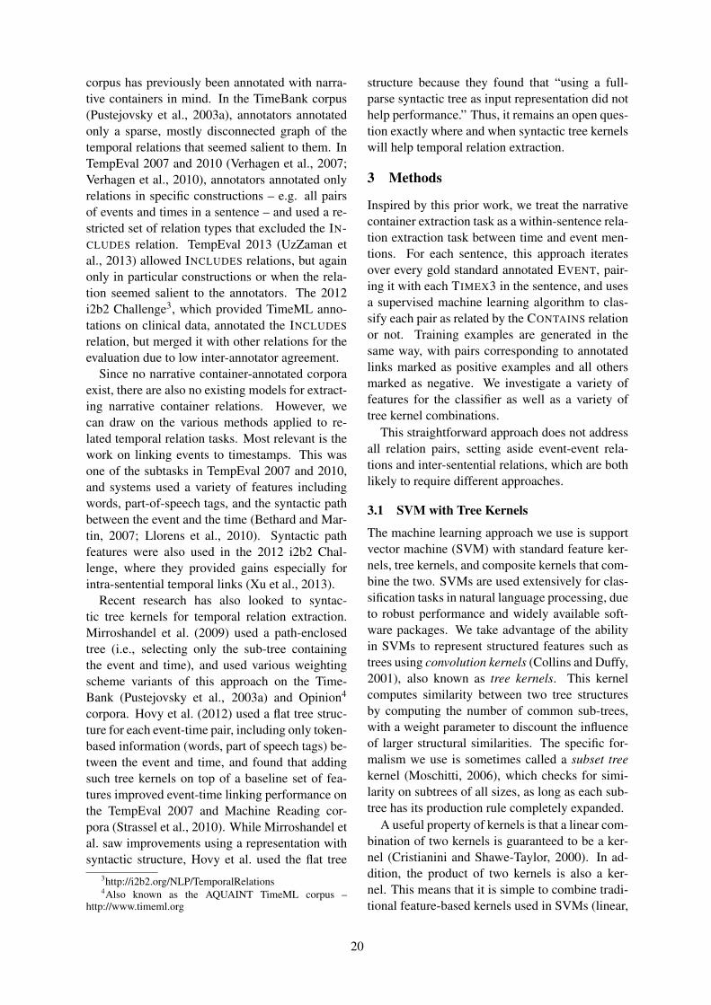
corpus has previously been annotated with narra-tive containers in mind. In the TimeBank corpus(Pustejovsky et al., 2003a), annotators annotatedonly a sparse, mostly disconnected graph of thetemporal relations that seemed salient to them. InTempEval 2007 and 2010 (Verhagen et al., 2007;Verhagen et al., 2010), annotators annotated onlyrelations in specific constructions – e.g. all pairsof events and times in a sentence – and used a re-stricted set of relation types that excluded the IN-CLUDES relation. TempEval 2013 (UzZaman etal., 2013) allowed INCLUDES relations, but againonly in particular constructions or when the rela-tion seemed salient to the annotators. The 2012i2b2 Challenge3, which provided TimeML anno-tations on clinical data, annotated the INCLUDES
relation, but merged it with other relations for theevaluation due to low inter-annotator agreement.
Since no narrative container-annotated corporaexist, there are also no existing models for extract-ing narrative container relations. However, wecan draw on the various methods applied to re-lated temporal relation tasks. Most relevant is thework on linking events to timestamps. This wasone of the subtasks in TempEval 2007 and 2010,and systems used a variety of features includingwords, part-of-speech tags, and the syntactic pathbetween the event and the time (Bethard and Mar-tin, 2007; Llorens et al., 2010). Syntactic pathfeatures were also used in the 2012 i2b2 Chal-lenge, where they provided gains especially forintra-sentential temporal links (Xu et al., 2013).
Recent research has also looked to syntac-tic tree kernels for temporal relation extraction.Mirroshandel et al. (2009) used a path-enclosedtree (i.e., selecting only the sub-tree containingthe event and time), and used various weightingscheme variants of this approach on the Time-Bank (Pustejovsky et al., 2003a) and Opinion4
corpora. Hovy et al. (2012) used a flat tree struc-ture for each event-time pair, including only token-based information (words, part of speech tags) be-tween the event and time, and found that addingsuch tree kernels on top of a baseline set of fea-tures improved event-time linking performance onthe TempEval 2007 and Machine Reading cor-pora (Strassel et al., 2010). While Mirroshandel etal. saw improvements using a representation withsyntactic structure, Hovy et al. used the flat tree
3http://i2b2.org/NLP/TemporalRelations4Also known as the AQUAINT TimeML corpus –
http://www.timeml.org
structure because they found that “using a full-parse syntactic tree as input representation did nothelp performance.” Thus, it remains an open ques-tion exactly where and when syntactic tree kernelswill help temporal relation extraction.
3 Methods
Inspired by this prior work, we treat the narrativecontainer extraction task as a within-sentence rela-tion extraction task between time and event men-tions. For each sentence, this approach iteratesover every gold standard annotated EVENT, pair-ing it with each TIMEX3 in the sentence, and usesa supervised machine learning algorithm to clas-sify each pair as related by the CONTAINS relationor not. Training examples are generated in thesame way, with pairs corresponding to annotatedlinks marked as positive examples and all othersmarked as negative. We investigate a variety offeatures for the classifier as well as a variety oftree kernel combinations.
This straightforward approach does not addressall relation pairs, setting aside event-event rela-tions and inter-sentential relations, which are bothlikely to require different approaches.
3.1 SVM with Tree Kernels
The machine learning approach we use is supportvector machine (SVM) with standard feature ker-nels, tree kernels, and composite kernels that com-bine the two. SVMs are used extensively for clas-sification tasks in natural language processing, dueto robust performance and widely available soft-ware packages. We take advantage of the abilityin SVMs to represent structured features such astrees using convolution kernels (Collins and Duffy,2001), also known as tree kernels. This kernelcomputes similarity between two tree structuresby computing the number of common sub-trees,with a weight parameter to discount the influenceof larger structural similarities. The specific for-malism we use is sometimes called a subset treekernel (Moschitti, 2006), which checks for simi-larity on subtrees of all sizes, as long as each sub-tree has its production rule completely expanded.
A useful property of kernels is that a linear com-bination of two kernels is guaranteed to be a ker-nel (Cristianini and Shawe-Taylor, 2000). In ad-dition, the product of two kernels is also a ker-nel. This means that it is simple to combine tradi-tional feature-based kernels used in SVMs (linear,
20
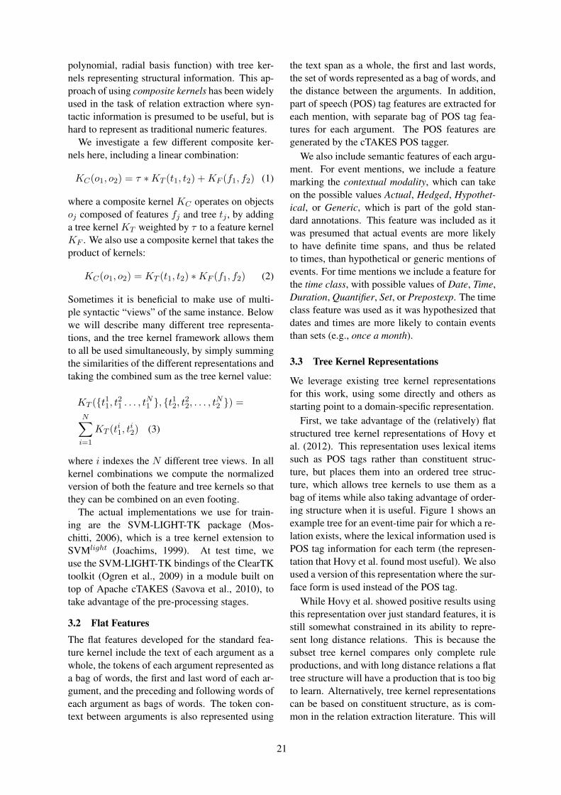
polynomial, radial basis function) with tree ker-nels representing structural information. This ap-proach of using composite kernels has been widelyused in the task of relation extraction where syn-tactic information is presumed to be useful, but ishard to represent as traditional numeric features.
We investigate a few different composite ker-nels here, including a linear combination:
KC(o1, o2) = τ ∗KT (t1, t2) +KF (f1, f2) (1)
where a composite kernel KC operates on objectsoj composed of features fj and tree tj , by addinga tree kernel KT weighted by τ to a feature kernelKF . We also use a composite kernel that takes theproduct of kernels:
KC(o1, o2) = KT (t1, t2) ∗KF (f1, f2) (2)
Sometimes it is beneficial to make use of multi-ple syntactic “views” of the same instance. Belowwe will describe many different tree representa-tions, and the tree kernel framework allows themto all be used simultaneously, by simply summingthe similarities of the different representations andtaking the combined sum as the tree kernel value:
KT ({t11, t21 . . . , tN1 }, {t12, t22, . . . , tN2 }) =
N∑i=1
KT (ti1, ti2) (3)
where i indexes the N different tree views. In allkernel combinations we compute the normalizedversion of both the feature and tree kernels so thatthey can be combined on an even footing.
The actual implementations we use for train-ing are the SVM-LIGHT-TK package (Mos-chitti, 2006), which is a tree kernel extension toSVMlight (Joachims, 1999). At test time, weuse the SVM-LIGHT-TK bindings of the ClearTKtoolkit (Ogren et al., 2009) in a module built ontop of Apache cTAKES (Savova et al., 2010), totake advantage of the pre-processing stages.
3.2 Flat FeaturesThe flat features developed for the standard fea-ture kernel include the text of each argument as awhole, the tokens of each argument represented asa bag of words, the first and last word of each ar-gument, and the preceding and following words ofeach argument as bags of words. The token con-text between arguments is also represented using
the text span as a whole, the first and last words,the set of words represented as a bag of words, andthe distance between the arguments. In addition,part of speech (POS) tag features are extracted foreach mention, with separate bag of POS tag fea-tures for each argument. The POS features aregenerated by the cTAKES POS tagger.
We also include semantic features of each argu-ment. For event mentions, we include a featuremarking the contextual modality, which can takeon the possible values Actual, Hedged, Hypothet-ical, or Generic, which is part of the gold stan-dard annotations. This feature was included as itwas presumed that actual events are more likelyto have definite time spans, and thus be relatedto times, than hypothetical or generic mentions ofevents. For time mentions we include a feature forthe time class, with possible values of Date, Time,Duration, Quantifier, Set, or Prepostexp. The timeclass feature was used as it was hypothesized thatdates and times are more likely to contain eventsthan sets (e.g., once a month).
3.3 Tree Kernel Representations
We leverage existing tree kernel representationsfor this work, using some directly and others asstarting point to a domain-specific representation.
First, we take advantage of the (relatively) flatstructured tree kernel representations of Hovy etal. (2012). This representation uses lexical itemssuch as POS tags rather than constituent struc-ture, but places them into an ordered tree struc-ture, which allows tree kernels to use them as abag of items while also taking advantage of order-ing structure when it is useful. Figure 1 shows anexample tree for an event-time pair for which a re-lation exists, where the lexical information used isPOS tag information for each term (the represen-tation that Hovy et al. found most useful). We alsoused a version of this representation where the sur-face form is used instead of the POS tag.
While Hovy et al. showed positive results usingthis representation over just standard features, it isstill somewhat constrained in its ability to repre-sent long distance relations. This is because thesubset tree kernel compares only complete ruleproductions, and with long distance relations a flattree structure will have a production that is too bigto learn. Alternatively, tree kernel representationscan be based on constituent structure, as is com-mon in the relation extraction literature. This will
21
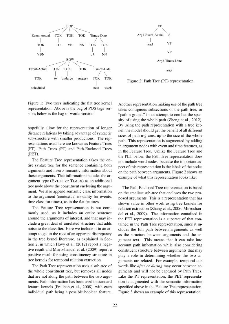
BOP
Event-Actual
TOK
VBN
TOK
TO
TOK
VB
TOK
NN
Timex-Date
TOK
JJ
TOK
NN
BOW
Event-Actual
TOK
scheduled
TOK
to
TOK
undergo
TOK
surgery
Timex-Date
TOK
next
TOK
week
Figure 1: Two trees indicating the flat tree kernelrepresentation. Above is the bag of POS tags ver-sion; below is the bag of words version.
hopefully allow for the representation of longerdistance relations by taking advantage of syntacticsub-structure with smaller productions. The rep-resentations used here are known as Feature Trees(FT), Path Trees (PT) and Path-Enclosed Trees(PET).
The Feature Tree representation takes the en-tire syntax tree for the sentence containing botharguments and inserts semantic information aboutthose arguments. That information includes the ar-gument type (EVENT or TIMEX) as an additionaltree node above the constituent enclosing the argu-ment. We also append semantic class informationto the argument (contextual modality for events,time class for times), as in the flat features.
The Feature Tree representation is not com-monly used, as it includes an entire sentencearound the arguments of interest, and that may in-clude a great deal of unrelated structure that addsnoise to the classifier. Here we include it in an at-tempt to get to the root of an apparent discrepancyin the tree kernel literature, as explained in Sec-tion 2, in which Hovy et al. (2012) report a nega-tive result and Mirroshandel et al. (2009) report apositive result for using constituency structure intree kernels for temporal relation extraction.
The Path Tree representation uses a sub-tree ofthe whole constituent tree, but removes all nodesthat are not along the path between the two argu-ments. Path information has been used in standardfeature kernels (Pradhan et al., 2008), with eachindividual path being a possible boolean feature.
VP
Arg1-Event-Actual
arg1
S
VP
VP
Arg2-Timex-Date
arg2
Figure 2: Path Tree (PT) representation
Another representation making use of the path treetakes contiguous subsections of the path tree, or“path n-grams,” in an attempt to combat the spar-sity of using the whole path (Zheng et al., 2012).By using the path representation with a tree ker-nel, the model should get the benefit of all differentsizes of path n-grams, up to the size of the wholepath. This representation is augmented by addingin argument nodes with event and time features, asin the Feature Tree. Unlike the Feature Tree andthe PET below, the Path Tree representation doesnot include word nodes, because the important as-pect of this representation is the labels of the nodeson the path between arguments. Figure 2 shows anexample of what this representation looks like.
The Path-Enclosed Tree representation is basedon the smallest sub-tree that encloses the two pro-posed arguments. This is a representation that hasshown value in other work using tree kernels forrelation extraction (Zhang et al., 2006; Mirroshan-del et al., 2009). The information contained inthe PET representation is a superset of that con-tained in the Path Tree representation, since it in-cludes the full path between arguments as wellas the structure between arguments and the ar-gument text. This means that it can take intoaccount path information while also consideringconstituent structure between arguments that mayplay a role in determining whether the two ar-guments are related. For example, temporal cuewords like after or during may occur between ar-guments and will not be captured by Path Trees.Like the PT representation, the PET representa-tion is augmented with the semantic informationspecified above in the Feature Tree representation.Figure 3 shows an example of this representation.
22
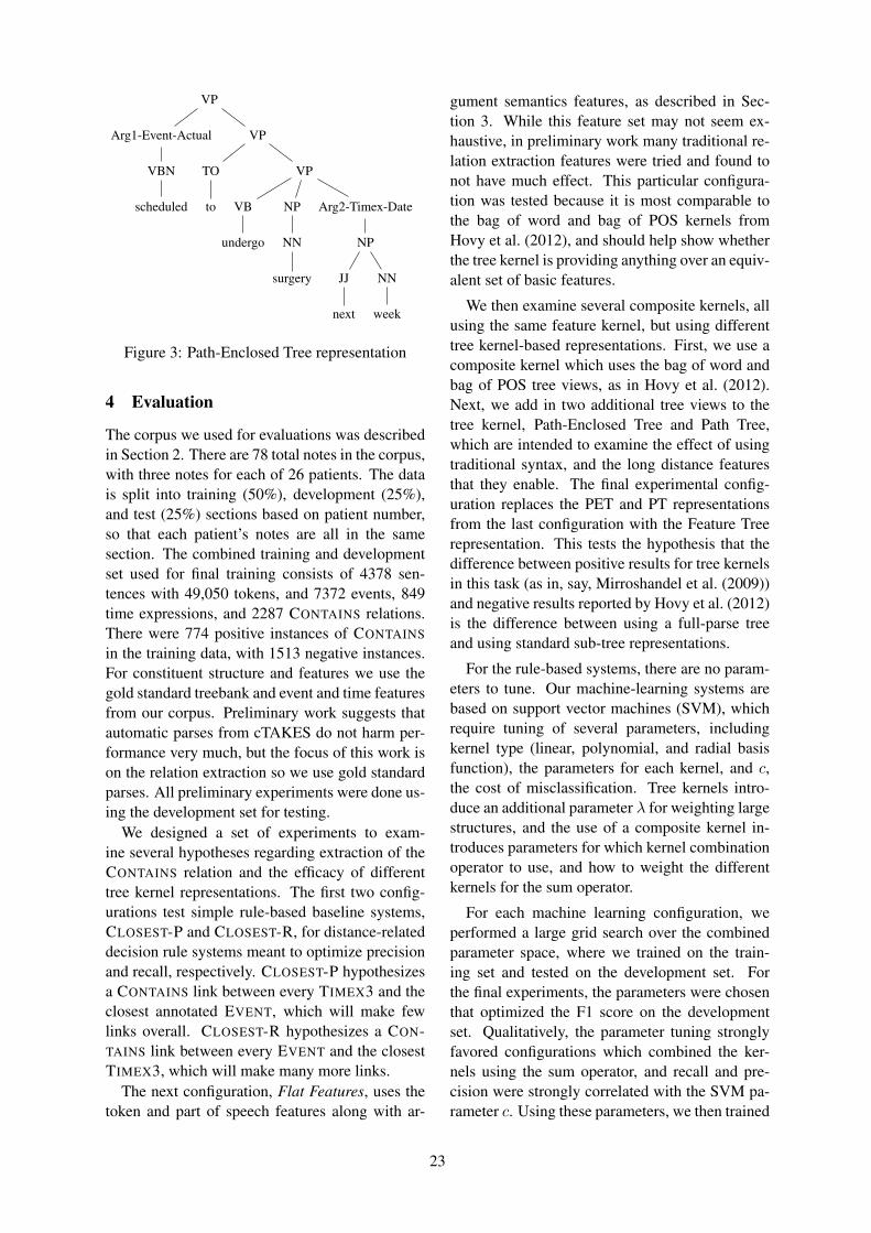
VP
Arg1-Event-Actual
VBN
scheduled
VP
TO
to
VP
VB
undergo
NP
NN
surgery
Arg2-Timex-Date
NP
JJ
next
NN
week
Figure 3: Path-Enclosed Tree representation
4 Evaluation
The corpus we used for evaluations was describedin Section 2. There are 78 total notes in the corpus,with three notes for each of 26 patients. The datais split into training (50%), development (25%),and test (25%) sections based on patient number,so that each patient’s notes are all in the samesection. The combined training and developmentset used for final training consists of 4378 sen-tences with 49,050 tokens, and 7372 events, 849time expressions, and 2287 CONTAINS relations.There were 774 positive instances of CONTAINS
in the training data, with 1513 negative instances.For constituent structure and features we use thegold standard treebank and event and time featuresfrom our corpus. Preliminary work suggests thatautomatic parses from cTAKES do not harm per-formance very much, but the focus of this work ison the relation extraction so we use gold standardparses. All preliminary experiments were done us-ing the development set for testing.
We designed a set of experiments to exam-ine several hypotheses regarding extraction of theCONTAINS relation and the efficacy of differenttree kernel representations. The first two config-urations test simple rule-based baseline systems,CLOSEST-P and CLOSEST-R, for distance-relateddecision rule systems meant to optimize precisionand recall, respectively. CLOSEST-P hypothesizesa CONTAINS link between every TIMEX3 and theclosest annotated EVENT, which will make fewlinks overall. CLOSEST-R hypothesizes a CON-TAINS link between every EVENT and the closestTIMEX3, which will make many more links.
The next configuration, Flat Features, uses thetoken and part of speech features along with ar-
gument semantics features, as described in Sec-tion 3. While this feature set may not seem ex-haustive, in preliminary work many traditional re-lation extraction features were tried and found tonot have much effect. This particular configura-tion was tested because it is most comparable tothe bag of word and bag of POS kernels fromHovy et al. (2012), and should help show whetherthe tree kernel is providing anything over an equiv-alent set of basic features.
We then examine several composite kernels, allusing the same feature kernel, but using differenttree kernel-based representations. First, we use acomposite kernel which uses the bag of word andbag of POS tree views, as in Hovy et al. (2012).Next, we add in two additional tree views to thetree kernel, Path-Enclosed Tree and Path Tree,which are intended to examine the effect of usingtraditional syntax, and the long distance featuresthat they enable. The final experimental config-uration replaces the PET and PT representationsfrom the last configuration with the Feature Treerepresentation. This tests the hypothesis that thedifference between positive results for tree kernelsin this task (as in, say, Mirroshandel et al. (2009))and negative results reported by Hovy et al. (2012)is the difference between using a full-parse treeand using standard sub-tree representations.
For the rule-based systems, there are no param-eters to tune. Our machine-learning systems arebased on support vector machines (SVM), whichrequire tuning of several parameters, includingkernel type (linear, polynomial, and radial basisfunction), the parameters for each kernel, and c,the cost of misclassification. Tree kernels intro-duce an additional parameter λ for weighting largestructures, and the use of a composite kernel in-troduces parameters for which kernel combinationoperator to use, and how to weight the differentkernels for the sum operator.
For each machine learning configuration, weperformed a large grid search over the combinedparameter space, where we trained on the train-ing set and tested on the development set. Forthe final experiments, the parameters were chosenthat optimized the F1 score on the developmentset. Qualitatively, the parameter tuning stronglyfavored configurations which combined the ker-nels using the sum operator, and recall and pre-cision were strongly correlated with the SVM pa-rameter c. Using these parameters, we then trained
23
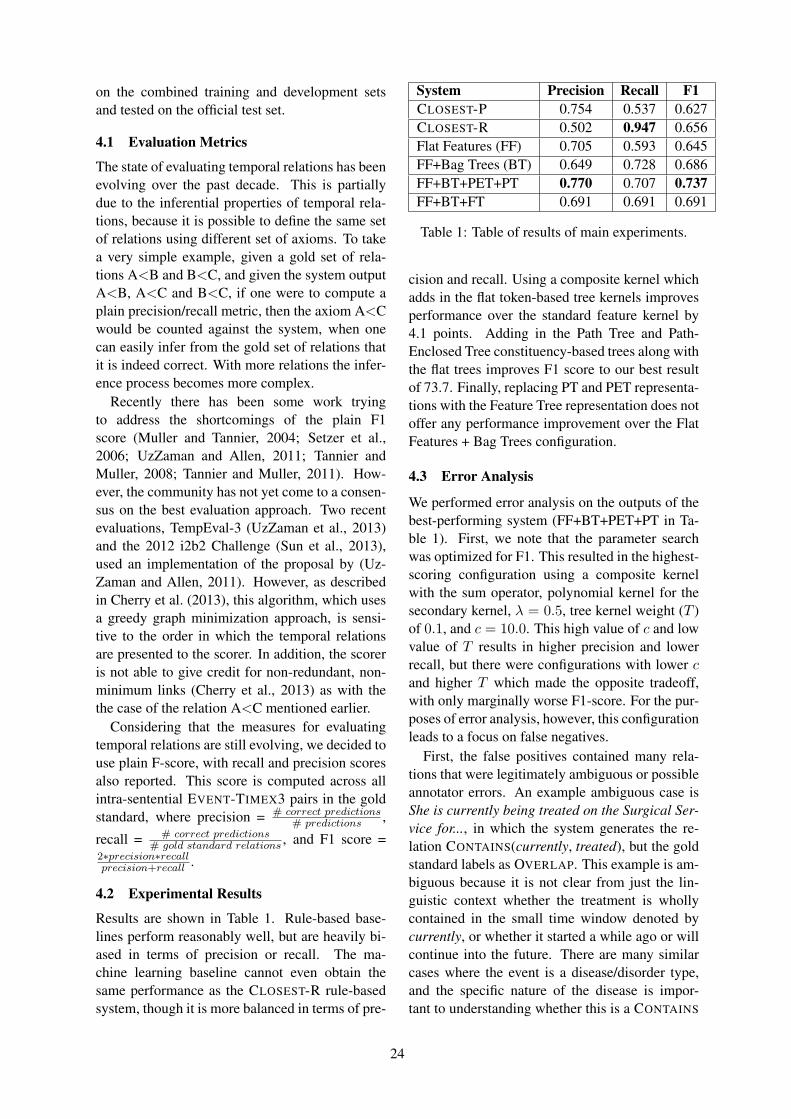
on the combined training and development setsand tested on the official test set.
4.1 Evaluation Metrics
The state of evaluating temporal relations has beenevolving over the past decade. This is partiallydue to the inferential properties of temporal rela-tions, because it is possible to define the same setof relations using different set of axioms. To takea very simple example, given a gold set of rela-tions A<B and B<C, and given the system outputA<B, A<C and B<C, if one were to compute aplain precision/recall metric, then the axiom A<Cwould be counted against the system, when onecan easily infer from the gold set of relations thatit is indeed correct. With more relations the infer-ence process becomes more complex.
Recently there has been some work tryingto address the shortcomings of the plain F1score (Muller and Tannier, 2004; Setzer et al.,2006; UzZaman and Allen, 2011; Tannier andMuller, 2008; Tannier and Muller, 2011). How-ever, the community has not yet come to a consen-sus on the best evaluation approach. Two recentevaluations, TempEval-3 (UzZaman et al., 2013)and the 2012 i2b2 Challenge (Sun et al., 2013),used an implementation of the proposal by (Uz-Zaman and Allen, 2011). However, as describedin Cherry et al. (2013), this algorithm, which usesa greedy graph minimization approach, is sensi-tive to the order in which the temporal relationsare presented to the scorer. In addition, the scoreris not able to give credit for non-redundant, non-minimum links (Cherry et al., 2013) as with thethe case of the relation A<C mentioned earlier.
Considering that the measures for evaluatingtemporal relations are still evolving, we decided touse plain F-score, with recall and precision scoresalso reported. This score is computed across allintra-sentential EVENT-TIMEX3 pairs in the goldstandard, where precision = # correct predictions
# predictions ,
recall = # correct predictions# gold standard relations , and F1 score =
2∗precision∗recallprecision+recall .
4.2 Experimental Results
Results are shown in Table 1. Rule-based base-lines perform reasonably well, but are heavily bi-ased in terms of precision or recall. The ma-chine learning baseline cannot even obtain thesame performance as the CLOSEST-R rule-basedsystem, though it is more balanced in terms of pre-
System Precision Recall F1CLOSEST-P 0.754 0.537 0.627CLOSEST-R 0.502 0.947 0.656Flat Features (FF) 0.705 0.593 0.645FF+Bag Trees (BT) 0.649 0.728 0.686FF+BT+PET+PT 0.770 0.707 0.737FF+BT+FT 0.691 0.691 0.691
Table 1: Table of results of main experiments.
cision and recall. Using a composite kernel whichadds in the flat token-based tree kernels improvesperformance over the standard feature kernel by4.1 points. Adding in the Path Tree and Path-Enclosed Tree constituency-based trees along withthe flat trees improves F1 score to our best resultof 73.7. Finally, replacing PT and PET representa-tions with the Feature Tree representation does notoffer any performance improvement over the FlatFeatures + Bag Trees configuration.
4.3 Error Analysis
We performed error analysis on the outputs of thebest-performing system (FF+BT+PET+PT in Ta-ble 1). First, we note that the parameter searchwas optimized for F1. This resulted in the highest-scoring configuration using a composite kernelwith the sum operator, polynomial kernel for thesecondary kernel, λ = 0.5, tree kernel weight (T )of 0.1, and c = 10.0. This high value of c and lowvalue of T results in higher precision and lowerrecall, but there were configurations with lower cand higher T which made the opposite tradeoff,with only marginally worse F1-score. For the pur-poses of error analysis, however, this configurationleads to a focus on false negatives.
First, the false positives contained many rela-tions that were legitimately ambiguous or possibleannotator errors. An example ambiguous case isShe is currently being treated on the Surgical Ser-vice for..., in which the system generates the re-lation CONTAINS(currently, treated), but the goldstandard labels as OVERLAP. This example is am-biguous because it is not clear from just the lin-guistic context whether the treatment is whollycontained in the small time window denoted bycurrently, or whether it started a while ago or willcontinue into the future. There are many similarcases where the event is a disease/disorder type,and the specific nature of the disease is impor-tant to understanding whether this is a CONTAINS
24
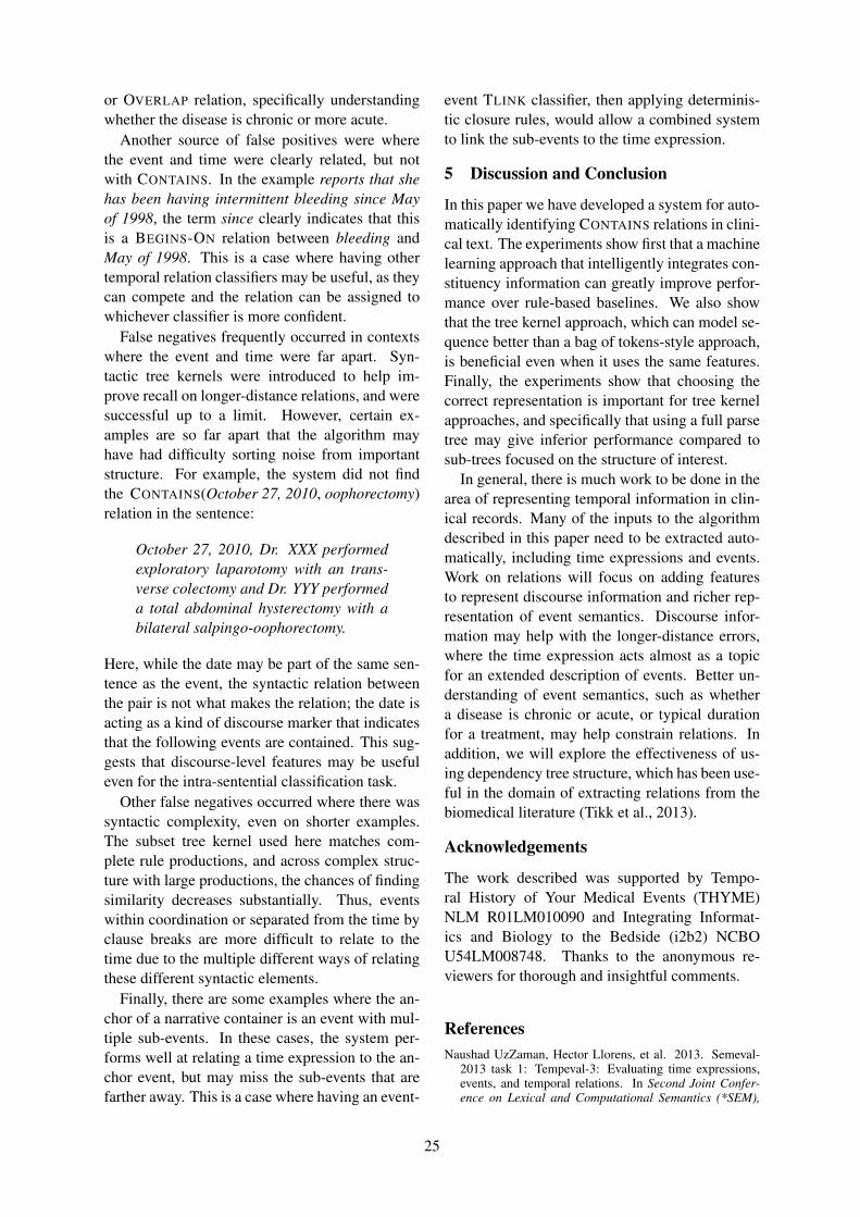
or OVERLAP relation, specifically understandingwhether the disease is chronic or more acute.
Another source of false positives were wherethe event and time were clearly related, but notwith CONTAINS. In the example reports that shehas been having intermittent bleeding since Mayof 1998, the term since clearly indicates that thisis a BEGINS-ON relation between bleeding andMay of 1998. This is a case where having othertemporal relation classifiers may be useful, as theycan compete and the relation can be assigned towhichever classifier is more confident.
False negatives frequently occurred in contextswhere the event and time were far apart. Syn-tactic tree kernels were introduced to help im-prove recall on longer-distance relations, and weresuccessful up to a limit. However, certain ex-amples are so far apart that the algorithm mayhave had difficulty sorting noise from importantstructure. For example, the system did not findthe CONTAINS(October 27, 2010, oophorectomy)relation in the sentence:
October 27, 2010, Dr. XXX performedexploratory laparotomy with an trans-verse colectomy and Dr. YYY performeda total abdominal hysterectomy with abilateral salpingo-oophorectomy.
Here, while the date may be part of the same sen-tence as the event, the syntactic relation betweenthe pair is not what makes the relation; the date isacting as a kind of discourse marker that indicatesthat the following events are contained. This sug-gests that discourse-level features may be usefuleven for the intra-sentential classification task.
Other false negatives occurred where there wassyntactic complexity, even on shorter examples.The subset tree kernel used here matches com-plete rule productions, and across complex struc-ture with large productions, the chances of findingsimilarity decreases substantially. Thus, eventswithin coordination or separated from the time byclause breaks are more difficult to relate to thetime due to the multiple different ways of relatingthese different syntactic elements.
Finally, there are some examples where the an-chor of a narrative container is an event with mul-tiple sub-events. In these cases, the system per-forms well at relating a time expression to the an-chor event, but may miss the sub-events that arefarther away. This is a case where having an event-
event TLINK classifier, then applying determinis-tic closure rules, would allow a combined systemto link the sub-events to the time expression.
5 Discussion and Conclusion
In this paper we have developed a system for auto-matically identifying CONTAINS relations in clini-cal text. The experiments show first that a machinelearning approach that intelligently integrates con-stituency information can greatly improve perfor-mance over rule-based baselines. We also showthat the tree kernel approach, which can model se-quence better than a bag of tokens-style approach,is beneficial even when it uses the same features.Finally, the experiments show that choosing thecorrect representation is important for tree kernelapproaches, and specifically that using a full parsetree may give inferior performance compared tosub-trees focused on the structure of interest.
In general, there is much work to be done in thearea of representing temporal information in clin-ical records. Many of the inputs to the algorithmdescribed in this paper need to be extracted auto-matically, including time expressions and events.Work on relations will focus on adding featuresto represent discourse information and richer rep-resentation of event semantics. Discourse infor-mation may help with the longer-distance errors,where the time expression acts almost as a topicfor an extended description of events. Better un-derstanding of event semantics, such as whethera disease is chronic or acute, or typical durationfor a treatment, may help constrain relations. Inaddition, we will explore the effectiveness of us-ing dependency tree structure, which has been use-ful in the domain of extracting relations from thebiomedical literature (Tikk et al., 2013).
Acknowledgements
The work described was supported by Tempo-ral History of Your Medical Events (THYME)NLM R01LM010090 and Integrating Informat-ics and Biology to the Bedside (i2b2) NCBOU54LM008748. Thanks to the anonymous re-viewers for thorough and insightful comments.
ReferencesNaushad UzZaman, Hector Llorens, et al. 2013. Semeval-
2013 task 1: Tempeval-3: Evaluating time expressions,events, and temporal relations. In Second Joint Confer-ence on Lexical and Computational Semantics (*SEM),
25
Volume 2: Proceedings of the Seventh International Work-shop on Semantic Evaluation (SemEval 2013), pages 1–9,Atlanta, Georgia, USA, June. Association for Computa-tional Linguistics.
Ashwin N Ananthakrishnan, Tianxi Cai, et al. 2013. Improv-ing case definition of Crohn’s disease and ulcerative col-itis in electronic medical records using natural languageprocessing: a novel informatics approach. Inflammatorybowel diseases.
Steven Bethard and James H. Martin. 2007. CU-TMP: Tem-poral relation classification using syntactic and semanticfeatures. In Proceedings of the 4th International Work-shop on Semantic Evaluations (SemEval-2007), pages129–132.
Colin Cherry, Xiaodan Zhu, et al. 2013. A la recherche dutemps perdu: extracting temporal relations from medicaltext in the 2012 i2b2 NLP challenge. Journal of the Amer-ican Medical Informatics Association, March.
Michael Collins and Nigel Duffy. 2001. Convolution kernelsfor natural language. In Neural Information ProcessingSystems.
Nello Cristianini and John Shawe-Taylor. 2000. An Introduc-tion to Support Vector Machines and Other Kernel-basedLearning Methods. Cambridge University Press.
Dirk Hovy, James Fan, et al. 2012. When did that happen?:linking events and relations to timestamps. In Proceedingsof the 13th Conference of the European Chapter of the As-sociation for Computational Linguistics, pages 185–193.Association for Computational Linguistics.
Thorsten Joachims. 1999. Making large scale svm learningpractical. In B. Schlkopf, C. Burges, and A. Smola, edi-tors, Advances in Kernel Methods - Support Vector Learn-ing. Universitat Dortmund.
Chen Lin, Helena Canhao, et al. 2012. Feature engineeringand selection for rheumatoid arthritis disease activity clas-sification using electronic medical records. In Proceed-ings of ICML Workshop on Machine Learning for ClinicalData.
Hector Llorens, Estela Saquete, and Borja Navarro. 2010.TIPSem (english and spanish): Evaluating crfs and seman-tic roles in tempeval-2. In Proceedings of the 5th Interna-tional Workshop on Semantic Evaluation, pages 284–291.Association for Computational Linguistics.
Seyed Abolghasem Mirroshandel, M Khayyamian, andGR Ghassem-Sani. 2009. Using tree kernels for clas-sifying temporal relations between events. Proc. of thePACLIC23, pages 355–364.
Alessandro Moschitti. 2006. Efficient convolution kernelsfor dependency and constituent syntactic trees. In Ma-chine Learning: ECML 2006, pages 318–329. Springer.
Philippe Muller and Xavier Tannier. 2004. Annotating andmeasuring temporal relations in texts. In Proceedings ofthe 20th international conference on Computational Lin-guistics, COLING ’04, Stroudsburg, PA, USA. Associa-tion for Computational Linguistics.
Philip V. Ogren, Philipp G. Wetzler, and Steven J. Bethard.2009. ClearTK: a framework for statistical natural lan-guage processing. In Unstructured Information Manage-ment Architecture Workshop at the Conference of the Ger-man Society for Computational Linguistics and LanguageTechnology, 9.
Sameer S Pradhan, Wayne Ward, and James H Martin. 2008.Towards robust semantic role labeling. ComputationalLinguistics, 34(2):289–310.
James Pustejovsky and Amber Stubbs. 2011. Increasing in-formativeness in temporal annotation. In Proceedings ofthe 5th Linguistic Annotation Workshop, pages 152–160.
James Pustejovsky, Patrick Hanks, et al. 2003a. The time-bank corpus. In Corpus linguistics, volume 2003, page 40.
James Pustejovsky, Jose Casta no, et al. 2003b. Timeml:Robust specification of event and temporal expressions intext. In Fifth International Workshop on ComputationalSemantics (IWCS-5).
Preethi Raghavan, Eric Fosler-Lussier, and Albert M Lai.2012. Temporal classification of medical events. In Pro-ceedings of the 2012 Workshop on Biomedical NaturalLanguage Processing, pages 29–37. Association for Com-putational Linguistics.
Guergana K. Savova, James J. Masanz, et al. 2010. Mayoclinical text analysis and knowledge extraction system(cTAKES): architecture, component evaluation and appli-cations. J Am Med Inform Assoc, 17(5):507–513.
Andrea Setzer, Robert Gaizauskas, and Mark Hepple. 2006.The role of inference in the temporal annotation and anal-ysis of text. Language Resources and Evaluation, 39(2-3):243–265, February.
Stephanie Strassel, Dan Adams, et al. 2010. The DARPAmachine reading program - encouraging linguistic and rea-soning research with a series of reading tasks. In Proceed-ings of the Seventh International Conference on LanguageResources and Evaluation (LREC’10), Valletta, Malta.
Weiyi Sun, Anna Rumshisky, and Ozlem Uzuner. 2013.Evaluating temporal relations in clinical text: 2012 i2b2challenge. Journal of the American Medical InformaticsAssociation, April.
Xavier Tannier and Philippe Muller. 2008. Evaluation met-rics for automatic temporal annotation of texts. Proceed-ings of the Proceedings of the Sixth International Lan-guage Resources and Evaluation (LREC’08).
Xavier Tannier and Philippe Muller. 2011. Evaluating tem-poral graphs built from texts via transitive reduction. J.Artif. Int. Res., 40(1):375413, January.
Domonkos Tikk, Illes Solt, et al. 2013. A detailed error anal-ysis of 13 kernel methods for protein-protein interactionextraction. BMC bioinformatics, 14(1):12.
Naushad UzZaman and James Allen. 2011. Temporal eval-uation. In Proceedings of the 49th Annual Meeting of theAssociation for Computational Linguistics: Human Lan-guage Technologies, page 351–356.
Marc Verhagen, Robert Gaizauskas, et al. 2007. Semeval-2007 task 15: Tempeval temporal relation identification.In Proceedings of the Fourth International Workshop onSemantic Evaluations (SemEval-2007), pages 75–80.
Marc Verhagen, Roser Sauri, et al. 2010. Semeval-2010 task13: Tempeval-2. In Proceedings of the 5th InternationalWorkshop on Semantic Evaluation, pages 57–62, Uppsala,Sweden, July. Association for Computational Linguistics.
RA Wilke, H Xu, et al. 2011. The emerging role of electronicmedical records in pharmacogenomics. Clinical Pharma-cology & Therapeutics, 89(3):379–386.
Yan Xu, Yining Wang, et al. 2013. An end-to-end system toidentify temporal relation in discharge summaries: 2012i2b2 challenge. Journal of the American Medical Infor-matics Association : JAMIA.
Min Zhang, Jie Zhang, and Jian Su. 2006. Exploring syn-tactic features for relation extraction using a convolutiontree kernel. In Proceedings of the Human Language Tech-nology Conference of the North American Chapter of theACL, pages 288–295.
Jiaping Zheng, Wendy W Chapman, et al. 2012. A sys-tem for coreference resolution for the clinical narrative.Journal of the American Medical Informatics Association,19:660–667.
26
Proceedings of the 2013 Workshop on Biomedical Natural Language Processing (BioNLP 2013), pages 27–35,Sofia, Bulgaria, August 4-9 2013. c©2013 Association for Computational Linguistics
Identifying pathological findings in German radiology reports using asyntacto-semantic parsing approach
Claudia Bretschneider1,2, Sonja Zillner1 and Matthias Hammon3
1 Siemens AG, Corporate Technology, 81739 Munich, Germany2 University Munich, Center for Information and Language Processing, 80538 Munich, Germany
3 University Hospital Erlangen, Department of Radiology, 91054 Erlangen, Germany{claudia.bretschneider.ext,sonja.zillner}@siemens.com,
Abstract
In order to integrate heterogeneous clinicalinformation sources, semantically correlatinginformation entities have to be linked. Ourdiscussions with radiologists revealed thatanatomical entities with pathological findingsare of particular interest when linking radi-ology text and images. Previous research toidentify pathological findings focused on sim-plistic approaches that recognize diseases ornegated findings, but failed to establish a holis-tic approach. In this paper, we introduce oursyntacto-semantic parsing approach to clas-sify sentences in radiology reports as eitherpathological or non-pathological based on thefindings they describe. Although we operatewith an incomplete, RadLex-based linguisticresource, the obtained results show the effec-tiveness of our approach by identifying a recallvalue of 74.3% for the classification task.
1 Introduction
In radiology, descriptions of the patient’s health statusare stored in heterogeneous formats. They range fromradiology images - which are the primary source for ra-diologists - over dictated reports about the image find-ings up to written texts.
Although the various data items describe the samestatus, they are distributed in non-linked systems. Thisis hindering the radiologist’s workflow. Especiallywhen reading reports, radiologists want to link backfrom the described finding (in the text) to the relatedbody location (in the images). Today, they establishthe link manually. This is obviously time-consumingwhen state-of-the-art imaging modalities deliver a massof stacked images.
In order to link radiology images and reports, eachinformation source needs to be annotated with seman-tic meta-information about the anatomical entities theydescribe. The necessary semantic image annotationsfor the integration have been made available as a resultof the Theseus MEDICO project (Seifert, 2010). Intro-duced algorithms automatically detect anatomical en-tities in radiology images and annotate those with thecorresponding RadLex IDs (Seifert et al., 2009). The
semantic annotations from the reports have to be in linewith those image annotations. Therefore, the final re-sult of the text analysis system need to be anatomicalannotations based on RadLex. We introduce a mecha-nism that extracts those semantic annotations from theradiology reports to enable the integration.
We identified three challenges, which a text analy-sis system has to consider when extracting the relevantanatomical entities from text:
1. The linguistic characteristics of the reports differsignificantly from standard free-text,
2. the underlying German linguistic resource (theRadLex taxonomy) is incomplete and
3. only a subset of the named anatomical entities inthe reports are relevant for annotating.
First, the special linguistic characteristics of the han-dled German reports have to be taken into account.While the linguistic characteristics English radiologyreports have been intensively studied (Friedman et al.,1994; Friedman et al., 2002; Sager et al., 1994), Ger-man ones are still a young research area. German re-ports are comparable to English ones when it comesto structural particularities. One can observe two char-acteristics in both languages: syntactic shortness andreduced semantic complexity. But the reports differ inrichness of the language used. German language is richin inflection form; the same is true for German medicallanguage. Additionally, clinical texts extend the vari-ety in inflection forms by introducing a huge amount ofGreek- and Latin-rooted vocabulary. Further linguisticparticularities will be introduced in a later section.
Second, the anatomical annotations will be es-tablished based on the controlled vocabulary of theRadLex taxonomy. Anatomical annotations of the im-ages (based on RadLex) are already available and henceimpose the mandatory condition to use RadLex annota-tions for the reports. We operate on German radiologyreports that is why we use the German RadLex taxon-omy. Compared to the English version, the GermanRadLex is lacking in terminology. This is an obstacle,we have to overcome.
Third, we have to find a way to filter relevantanatomical annotations. According to the radiolo-gists we worked with, it is inappropriate to extract all
27
anatomical entities from the text to link them with theimage annotations. A large portion of the anatomiesis described with normal or absent findings, which donot describe pathologies. Those findings are includedin the reports in order to exclude differential diag-noses. However, radiologists are interested in imagesof anatomical entities described with pathological find-ings. Thus, a crucial part of our work is to extract theanatomical entities with pathological findings in orderto link only those with the image positions.
The core contribution of this paper is the descrip-tion of a syntacto-semantic parsing approach to identifythe sentences that describe pathological findings by us-ing the German version of the RadLex taxonomy. Theresults of this approach are used to integrate relevantsemantic information from heterogeneous data sourcesand support radiologists significantly in their work rou-tine.
To introduce our solution, the remainder of this pa-per is organized as follows: Section 2 refers to relatedwork in the field and shows where sub-problems arestill unsolved. In Section 3, we analyze the linguisticcharacteristics of the reports. Section 4 introduces thetext analysis system for integrating radiology text andimages. The system handles both the linguistic partic-ularities of the reports and the shortcomings of RadLexas linguistic resource and filters relevant anatomical en-tities from the reports. Section 5 evaluates and dis-cusses the classification and extraction results. Finally,Section 6 concludes with possible future work.
2 Related work
Medical grammar-based text analysis systems In-formation extraction from medical texts is a well-researched task in medical natural language processing(Meystre et al, 2008). Especially radiology reports playan important role.
Theoretical work in the linguistic characteristics ofthe medical sublanguage has been conducted on theadaption of theories of Harris by (Friedman et al.,2002). Early systems of (Sager et al., 1994; Friedmanet al., 1994) are adaptations of the theories and imple-ment own (context-free) medical language grammar forradiology reports. They show that parsing of medicaltexts based on a combined semantic-syntactic grammarcan be successfully conducted – but they conductedtheir research using English reports. Even today, ad-vances in grammar-based parsing of medical texts arereached (Fan et al., 2011).
More recently, sophisticated semantic medical textanalysis systems have integrated a component to parsetexts. (Savova et al., 2010) They take the output of theparsing process to extract semantic relationships be-tween the medical concepts described.
All those systems work with elaborated lexicons thatfully cover the vocabulary used in English report.
Detecting diseases and Negated finding Most sys-tems cover the problem of detecting pathological find-ings in the reports just partially: In order to detectpathologies, they automate the assignment of codes fordiseases listed in ontologies such as UMLS (Aronson,2001; Lindberg, 1990; Long, 2005) or ICD (Computa-tional Medicine Center, 2007; Pestian et al., 2007).
Non-pathological findings are identified using nega-tion detection algorithms. Available approaches rangefrom simple algorithms based on dictionary lookup andregular expressions (Chapman et al., 2001; Mutalik etal., 2001) through machine learning (Goryachev et al.,2006) up to advanced approaches that apply a context-free ”negation grammar” (Huang, 2007).
Gap analysis While the grammar-based analysis ofradiology reports has proven to be successful with com-plete lexical resources, we have to face the shortcom-ings of an incomplete lexicon. Furthermore, in othersystems the grammar is used to analyze the syntax ofthe reports. Our approach to use it for classification isnovel and has not been applied so far.
Working with German clinical texts is another chal-lenge in the field. English texts have been made avail-able by a number of shared tasks and gained more andmore interest in the last decade. Medical corpora inlanguages other than English are not available to thatextent.
That is perhaps also the reason for the tremendouslack of German medical ontologies. While great effortis put into the advance of English ontologies, Germanlanguage versions are rare.
Terminology acquisition and semantic classificationSemantic classifications beyond the hierarchical infor-mation encoded in taxonomies and ontologies are stillrare for ontology concepts. In particular, semantic clas-sifications such as information about the pathologicalnature of the concepts are missing so far.
Several approaches address this lack of semantic in-formation: Corpus-based approaches base their meth-ods on statistical analyses about the coverage and us-age frequency of UMLS ontology concepts (Liu et al.,2012; Wu et al., 2012). (Johnson, 1999) derives seman-tic classes from ontology mapping and disambiguatesmultiple senses in contexts of discharge summaries.(Campbell et al., 1999) applies pattern-based rules andcombines them with UMLS concepts to acquire newand semantically classified terminology. However, thisapproach is limited to noun phrases.
Finally, (Zweigenbaum et al., 2003) introduce ap-proaches to automatically extending the existing En-glish UMLS ontology with non-English concepts basedon statistical algorithms.
3 Corpus analysis3.1 Reference corpusSince a publicly available corpus of German radiologyreports is missing, we build our own annotated corpus
28
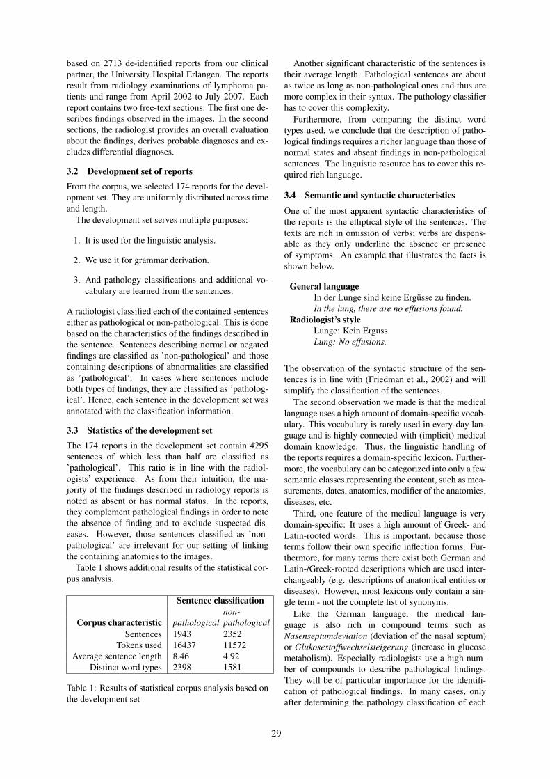
based on 2713 de-identified reports from our clinicalpartner, the University Hospital Erlangen. The reportsresult from radiology examinations of lymphoma pa-tients and range from April 2002 to July 2007. Eachreport contains two free-text sections: The first one de-scribes findings observed in the images. In the secondsections, the radiologist provides an overall evaluationabout the findings, derives probable diagnoses and ex-cludes differential diagnoses.
3.2 Development set of reportsFrom the corpus, we selected 174 reports for the devel-opment set. They are uniformly distributed across timeand length.
The development set serves multiple purposes:
1. It is used for the linguistic analysis.
2. We use it for grammar derivation.
3. And pathology classifications and additional vo-cabulary are learned from the sentences.
A radiologist classified each of the contained sentenceseither as pathological or non-pathological. This is donebased on the characteristics of the findings described inthe sentence. Sentences describing normal or negatedfindings are classified as ’non-pathological’ and thosecontaining descriptions of abnormalities are classifiedas ’pathological’. In cases where sentences includeboth types of findings, they are classified as ’patholog-ical’. Hence, each sentence in the development set wasannotated with the classification information.
3.3 Statistics of the development setThe 174 reports in the development set contain 4295sentences of which less than half are classified as’pathological’. This ratio is in line with the radiol-ogists’ experience. As from their intuition, the ma-jority of the findings described in radiology reports isnoted as absent or has normal status. In the reports,they complement pathological findings in order to notethe absence of finding and to exclude suspected dis-eases. However, those sentences classified as ’non-pathological’ are irrelevant for our setting of linkingthe containing anatomies to the images.
Table 1 shows additional results of the statistical cor-pus analysis.
Sentence classificationnon-
Corpus characteristic pathological pathologicalSentences 1943 2352
Tokens used 16437 11572Average sentence length 8.46 4.92
Distinct word types 2398 1581
Table 1: Results of statistical corpus analysis based onthe development set
Another significant characteristic of the sentences istheir average length. Pathological sentences are aboutas twice as long as non-pathological ones and thus aremore complex in their syntax. The pathology classifierhas to cover this complexity.
Furthermore, from comparing the distinct wordtypes used, we conclude that the description of patho-logical findings requires a richer language than those ofnormal states and absent findings in non-pathologicalsentences. The linguistic resource has to cover this re-quired rich language.
3.4 Semantic and syntactic characteristics
One of the most apparent syntactic characteristics ofthe reports is the elliptical style of the sentences. Thetexts are rich in omission of verbs; verbs are dispens-able as they only underline the absence or presenceof symptoms. An example that illustrates the facts isshown below.
General languageIn der Lunge sind keine Ergusse zu finden.In the lung, there are no effusions found.
Radiologist’s styleLunge: Kein Erguss.Lung: No effusions.
The observation of the syntactic structure of the sen-tences is in line with (Friedman et al., 2002) and willsimplify the classification of the sentences.
The second observation we made is that the medicallanguage uses a high amount of domain-specific vocab-ulary. This vocabulary is rarely used in every-day lan-guage and is highly connected with (implicit) medicaldomain knowledge. Thus, the linguistic handling ofthe reports requires a domain-specific lexicon. Further-more, the vocabulary can be categorized into only a fewsemantic classes representing the content, such as mea-surements, dates, anatomies, modifier of the anatomies,diseases, etc.
Third, one feature of the medical language is verydomain-specific: It uses a high amount of Greek- andLatin-rooted words. This is important, because thoseterms follow their own specific inflection forms. Fur-thermore, for many terms there exist both German andLatin-/Greek-rooted descriptions which are used inter-changeably (e.g. descriptions of anatomical entities ordiseases). However, most lexicons only contain a sin-gle term - not the complete list of synonyms.
Like the German language, the medical lan-guage is also rich in compound terms such asNasenseptumdeviation (deviation of the nasal septum)or Glukosestoffwechselsteigerung (increase in glucosemetabolism). Especially radiologists use a high num-ber of compounds to describe pathological findings.They will be of particular importance for the identifi-cation of pathological findings. In many cases, onlyafter determining the pathology classification of each
29
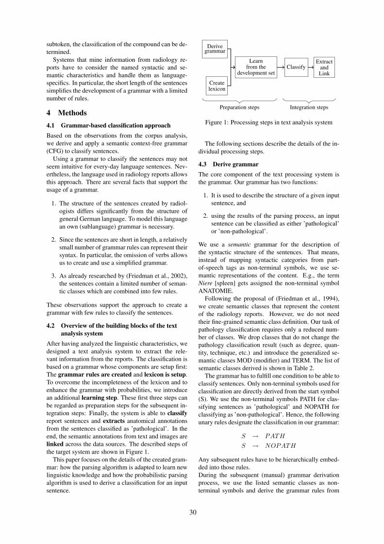
subtoken, the classification of the compound can be de-termined.
Systems that mine information from radiology re-ports have to consider the named syntactic and se-mantic characteristics and handle them as language-specifics. In particular, the short length of the sentencessimplifies the development of a grammar with a limitednumber of rules.
4 Methods4.1 Grammar-based classification approachBased on the observations from the corpus analysis,we derive and apply a semantic context-free grammar(CFG) to classify sentences.
Using a grammar to classify the sentences may notseem intuitive for every-day language sentences. Nev-ertheless, the language used in radiology reports allowsthis approach. There are several facts that support theusage of a grammar.
1. The structure of the sentences created by radiol-ogists differs significantly from the structure ofgeneral German language. To model this languagean own (sublanguage) grammar is necessary.
2. Since the sentences are short in length, a relativelysmall number of grammar rules can represent theirsyntax. In particular, the omission of verbs allowsus to create and use a simplified grammar.
3. As already researched by (Friedman et al., 2002),the sentences contain a limited number of seman-tic classes which are combined into few rules.
These observations support the approach to create agrammar with few rules to classify the sentences.
4.2 Overview of the building blocks of the textanalysis system
After having analyzed the linguistic characteristics, wedesigned a text analysis system to extract the rele-vant information from the reports. The classification isbased on a grammar whose components are setup first:The grammar rules are created and lexicon is setup.To overcome the incompleteness of the lexicon and toenhance the grammar with probabilities, we introducean additional learning step. These first three steps canbe regarded as preparation steps for the subsequent in-tegration steps: Finally, the system is able to classifyreport sentences and extracts anatomical annotationsfrom the sentences classified as ’pathological’. In theend, the semantic annotations from text and images arelinked across the data sources. The described steps ofthe target system are shown in Figure 1.
This paper focuses on the details of the created gram-mar: how the parsing algorithm is adapted to learn newlinguistic knowledge and how the probabilistic parsingalgorithm is used to derive a classification for an inputsentence.
Derivegrammar
Createlexicon
Learnfrom the
development set
Preparation steps
ClassifyExtract
andLink
Integration steps
Figure 1: Processing steps in text analysis system
The following sections describe the details of the in-dividual processing steps.
4.3 Derive grammarThe core component of the text processing system isthe grammar. Our grammar has two functions:
1. It is used to describe the structure of a given inputsentence, and
2. using the results of the parsing process, an inputsentence can be classified as either ’pathological’or ’non-pathological’.
We use a semantic grammar for the description ofthe syntactic structure of the sentences. That means,instead of mapping syntactic categories from part-of-speech tags as non-terminal symbols, we use se-mantic representations of the content. E.g., the termNiere [spleen] gets assigned the non-terminal symbolANATOMIE.
Following the proposal of (Friedman et al., 1994),we create semantic classes that represent the contentof the radiology reports. However, we do not needtheir fine-grained semantic class definition. Our task ofpathology classification requires only a reduced num-ber of classes. We drop classes that do not change thepathology classification result (such as degree, quan-tity, technique, etc.) and introduce the generalized se-mantic classes MOD (modifier) and TERM. The list ofsemantic classes derived is shown in Table 2.
The grammar has to fulfill one condition to be able toclassify sentences. Only non-terminal symbols used forclassification are directly derived from the start symbol(S). We use the non-terminal symbols PATH for clas-sifying sentences as ’pathological’ and NOPATH forclassifying as ’non-pathological’. Hence, the followingunary rules designate the classification in our grammar:
S → PATH
S → NOPATH
Any subsequent rules have to be hierarchically embed-ded into those rules.During the subsequent (manual) grammar derivationprocess, we use the listed semantic classes as non-terminal symbols and derive the grammar rules from
30
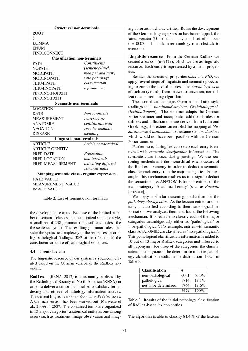
Structural non-terminalsROOTSKOMMAENUMFIND CONNECT
Classification non-terminalsPATH Constituents
(sentence-level,modifier and term)with pathologyclassificationinformation
NOPATHMOD PATHMOD NOPATHTERM PATHTERM NOPATHFINDING NOPATHFINDING PATH
Semantic non-terminalsLOCATION
Non-terminalsrepresentingconstituents withspecific semanticmeaning
DATEMEASUREMENTANATOMIENEGATIONDISEASE
Linguistic non-terminalsARTICLE Article non-terminalARTICLE GENITIVPREP DATE Preposition
non-terminalsindicating differentsemantic units
PREP LOCATIONPREP MEASUREMENT
Mapping semantic class - regular expressionDATE VALUEMEASUREMENT VALUEIMAGE VALUE
Table 2: List of semantic non-terminals
the development corpus. Because of the limited num-ber of semantic classes and the elliptical sentence style,a small set of 238 grammar rules suffices to describethe sentence syntax. The resulting grammar rules con-sider the syntactic complexity of the sentences describ-ing pathological findings: 52% of the rules model theconstituent structure of pathological sentences.
4.4 Create lexicon
The linguistic resource of our system is a lexicon, cre-ated based on the German version of the RadLex tax-onomy.
RadLex (RSNA, 2012) is a taxonomy published bythe Radiological Society of North America (RNSA) inorder to deliver a uniform controlled vocabulary for in-dexing and retrieval of radiology information sources.The current English version 3.8 contains 39976 classes.A German version has been worked-out (Marwede etal., 2009) in 2007. The contained terms are organizedin 13 major categories: anatomical entity as one amongothers such as treatment, image observation and imag-
ing observation characteristics. But as the developmentof the German language version has been stopped, thelatest version 2.0 contains only a subset of classes(n=10003). This lack in terminology is an obstacle toovercome.
Linguistic resource From the German RadLex wecreated a lexicon (n=9479), which we use as linguisticresource. Each entry is represented by a list of proper-ties.
Besides the structural properties label and RID, weapply several steps of linguistic and semantic process-ing to enrich the lexical entries. The normalized stemof each entry results from an own tokenization, normal-ization and stemming algorithm.
The normalization aligns German and Latin stylespellings (e.g. Karzinom/Carzinom, Okzipitallappen/-Occipitallappen). The stemmer adapts the GermanPorter stemmer and incorporates additional rules forsuffixes and inflection that are derived from Latin andGreek. E.g., this extension enabled the mapping of Me-diastinum and mediastinal to the same stem mediastin-,which would not have been possible with the GermanPorter stemmer.
Furthermore, during lexicon setup each entry is en-riched with semantic classification information. Thesemantic class is used during parsing. We use rea-soning methods and the hierarchical is-a structure ofthe RadLex taxonomy in order to deduct a semanticclass for each entry from the major categories. For ex-ample, this mechanism enables us to assign to deductthe semantic class ANATOMIE for sub-entities of themajor category ’Anatomical entity’ (such as Prostata[prostate]).
We apply a similar reasoning mechanism for thepathology classification. As the lexicon entries are ini-tially unclassified according to their pathological in-formation, we analyzed them and found the followingmechanism: It is feasible to classify each of the majorcategories unambiguously either as ’pathological’ or’non-pathological’. For example, entries with semanticclass ANATOMIE are classified as ’non-pathological’.This pathological classification information is added to10 out of 13 major RadLex categories and inferred toall hyponyms. For three of the categories, the classifi-cation is ambiguous. The determination of the pathol-ogy classification results in the distribution shown inTable 3.
Classification #non-pathological 6001 63.3%pathological 1714 18.1%not to be determined 1764 18.6%
9479 100%
Table 3: Results of the initial pathology classificationof RadLex-based lexicon entries
The algorithm is able to classify 81.4 % of the lexicon
31
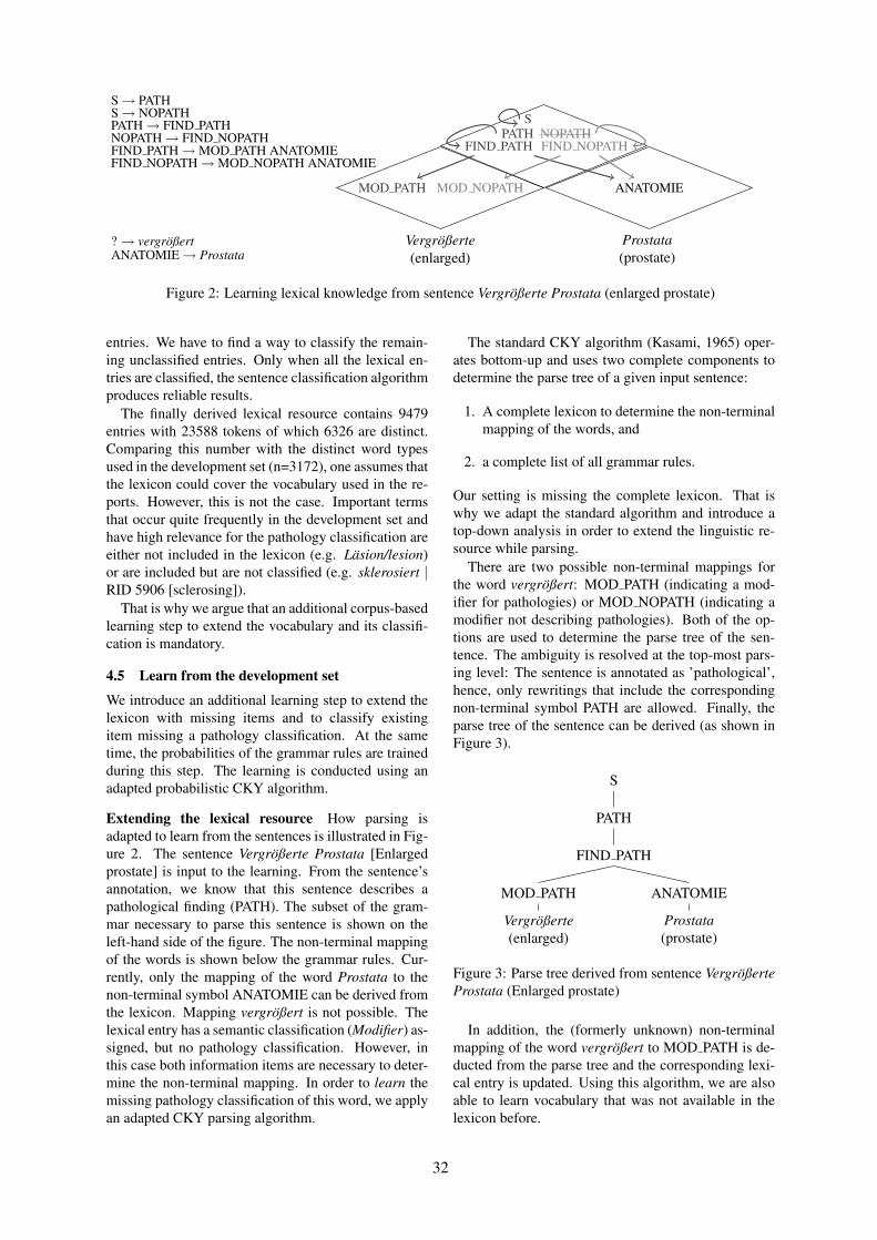
S→ PATHS→ NOPATHPATH→ FIND PATHNOPATH→ FIND NOPATHFIND PATH→MOD PATH ANATOMIEFIND NOPATH→MOD NOPATH ANATOMIE
? → vergroßertANATOMIE→ Prostata
Vergroßerte(enlarged)
Prostata(prostate)
MOD PATH MOD NOPATH ANATOMIE
FIND PATHPATH
FIND NOPATHNOPATH
S
Figure 2: Learning lexical knowledge from sentence Vergroßerte Prostata (enlarged prostate)
entries. We have to find a way to classify the remain-ing unclassified entries. Only when all the lexical en-tries are classified, the sentence classification algorithmproduces reliable results.
The finally derived lexical resource contains 9479entries with 23588 tokens of which 6326 are distinct.Comparing this number with the distinct word typesused in the development set (n=3172), one assumes thatthe lexicon could cover the vocabulary used in the re-ports. However, this is not the case. Important termsthat occur quite frequently in the development set andhave high relevance for the pathology classification areeither not included in the lexicon (e.g. Lasion/lesion)or are included but are not classified (e.g. sklerosiert |RID 5906 [sclerosing]).
That is why we argue that an additional corpus-basedlearning step to extend the vocabulary and its classifi-cation is mandatory.
4.5 Learn from the development set
We introduce an additional learning step to extend thelexicon with missing items and to classify existingitem missing a pathology classification. At the sametime, the probabilities of the grammar rules are trainedduring this step. The learning is conducted using anadapted probabilistic CKY algorithm.
Extending the lexical resource How parsing isadapted to learn from the sentences is illustrated in Fig-ure 2. The sentence Vergroßerte Prostata [Enlargedprostate] is input to the learning. From the sentence’sannotation, we know that this sentence describes apathological finding (PATH). The subset of the gram-mar necessary to parse this sentence is shown on theleft-hand side of the figure. The non-terminal mappingof the words is shown below the grammar rules. Cur-rently, only the mapping of the word Prostata to thenon-terminal symbol ANATOMIE can be derived fromthe lexicon. Mapping vergroßert is not possible. Thelexical entry has a semantic classification (Modifier) as-signed, but no pathology classification. However, inthis case both information items are necessary to deter-mine the non-terminal mapping. In order to learn themissing pathology classification of this word, we applyan adapted CKY parsing algorithm.
The standard CKY algorithm (Kasami, 1965) oper-ates bottom-up and uses two complete components todetermine the parse tree of a given input sentence:
1. A complete lexicon to determine the non-terminalmapping of the words, and
2. a complete list of all grammar rules.
Our setting is missing the complete lexicon. That iswhy we adapt the standard algorithm and introduce atop-down analysis in order to extend the linguistic re-source while parsing.
There are two possible non-terminal mappings forthe word vergroßert: MOD PATH (indicating a mod-ifier for pathologies) or MOD NOPATH (indicating amodifier not describing pathologies). Both of the op-tions are used to determine the parse tree of the sen-tence. The ambiguity is resolved at the top-most pars-ing level: The sentence is annotated as ’pathological’,hence, only rewritings that include the correspondingnon-terminal symbol PATH are allowed. Finally, theparse tree of the sentence can be derived (as shown inFigure 3).
S
PATH
FIND PATH
MOD PATH
Vergroßerte(enlarged)
ANATOMIE
Prostata(prostate)
Figure 3: Parse tree derived from sentence VergroßerteProstata (Enlarged prostate)
In addition, the (formerly unknown) non-terminalmapping of the word vergroßert to MOD PATH is de-ducted from the parse tree and the corresponding lexi-cal entry is updated. Using this algorithm, we are alsoable to learn vocabulary that was not available in thelexicon before.
32
Training the grammar’s probabilities The parsetree is also used as input for extending the grammarto a probabilistic context-free grammar. Each of thegrammar rules used to form the parse tree is used tore-calculate the probabilities of the grammar rules.
After the learning step, the lexicon is extended to10344 entries (before 9479). But even more impor-tant, the overall amount of lexicon entries classified as’pathological’ increased by 18.8 % to now 2036 entries(before 1714). We consider this a key success of thelearning, as our classification depends on this encodedknowledge.
4.6 ClassifyAfter conducting the previous steps,
1. the extended lexicon,
2. the trained P-CFG, and
3. the standard probabilistic CKY parsing algorithm
are applied to parse unclassified sentences.The sentence classification is conducted based on the
lexicon and the grammar rules. The lexicon helps to as-sign non-terminal symbols to the words in the sentence.Depending on non-terminal symbols assigned and thegrammar rules applied during the subsequent parsingprocess, the parse tree will reveal the classification ofthe sentence.
As parsing algorithm we apply the standard prob-abilistic CKY (P-CKY) algorithm. It resolves bothsyntactic and classification ambiguities. In case, thesentence contains unknown words, the probabilisticparsing feature helps to disambiguate the non-terminalassignment. The derived parse tree describes boththe syntactic structure of the sentence and the derivedpathology classification.
4.7 Extract and LinkFinally, in case a sentence is classified as ’patholog-ical’, the contained anatomical entities are extracted.The sentences are annotated with the extracted anatom-ical information. An external system combines theanatomical annotations from images and reports. Thus,links are created successfully and the correlating im-age positions for pathological findings can be accessedfrom the text.
5 EvaluationWe evaluate the classification system using 40randomly-chosen reports containing 1296 sentences.
5.1 Precision and recall measurementsWe evaluate the classification results and the successof the alignment of radiology reports and images usingprecision and recall values. Only for sentences classi-fied as ’pathological’, the contained anatomical entitiesare extracted and anatomical annotations are created.
That is why we prefer high recall values. If sentencesare misclassified as ’pathological’ – although they de-scribe non-pathological findings (FP) – this is a minorissue. This misclassification results in alignment ofanatomical entities in text and images without patho-logical findings. We accept lower precision values thatyield those additional, but not intended alignments.
5.2 Baseline evaluation
We compare the evaluation results of the classifica-tion system with the results of a semantically-informedbaseline algorithm. This algorithm detects nega-tions and classifies the containing sentences as ’non-pathological’. Sentences containing diseases (deter-mined based on Latin suffixes such as -itis, -ose, etc.)or a pathological RadLex concepts (as determined dur-ing the lexicon creation step) are classified as ’patho-logical’. Any remaining sentences are assumed to de-scribe non-pathological findings.
The results of the baseline classification are shownin Table 4. The headings denote ’non-pathological’sentences (NOPATH) respectively ’pathological’ sen-tences (PATH).
expected classificationPATH NOPATH
observed PATH 17 0classification NOPATH 446 833
Table 4: Classification results using baseline algorithm
This baseline approach has the advantage of 100% pre-cision value. However, it produces a low recall valueof 3.67 %, which shows that this approach is not appli-cable for the alignment of text and images. The resultsshow that the identification of pathologies is not feasi-ble by only using (1) suffixes to determine diseases and(2) available pathology descriptions from the RadLextaxonomy.
5.3 Evaluation of the parsing-based classificationresults
Table 5 shows the system results of classifying the 1296report sentences using the syntacto-semantic parsingapproach.
expected classificationPATH NOPATH
observed PATH 344 288classification NOPATH 119 545
Table 5: Sentence classification results using syntacto-semantic parsing approach
Taking into account the impact of the (still) incom-plete lexicon, the recall value of 74.3 % indicates thatthe chosen approach to classify pathological sentencesis successful. However, the precision value of 54.4 %
33
indicates that the classification of almost half of the’pathological’ sentences is incorrect.
Compared to the baseline, the acquisition of addi-tional, pathology classified vocabulary and its incorpo-ration into a parsing-based approach significantly im-proves the recall value. That is why we regard the en-richment of the lexicon at the crucial step for (further)improvement of the classification results. However, alarge amount of sentences was classified incorrectly as’pathological’. The error analysis will reveals somecauses.
5.4 Error analysisWe identified four error types that produce incorrectlyclassified results.
1. Some of the pathology classification of the seman-tic knowledge acquired during learning is incor-rect.
Terms that do not describe pathological proper-ties such as Voraufnahme [previous examination]or Lymphknoten [lymph node] were classified as’pathological’; also, pathological findings such asLasion [lesion] or Infiltrat [infiltrate] could not beclassified correctly. Because of their high usagefrequency (26, 116, 20, 7 times), these four termsare accountable for 169 of the misclassified sen-tences (both FP and FN) from the evaluation.
The disambiguation of (word-level) pathologyclassification using sentence-level annotations isobviously very vague and imprecise. In order toimprove the terminology acquisition results, wewill include distribution information and proba-bilistic features into the learning process as futurework.
2. The terminology acquisition leads to an extendedlexicon, but still, terminology remains uncovered.In particular, the description of pathological find-ings requires a richer language, its lack inhibitstheir correct classification. Even though our cor-pus is limited to reports of lymphoma patients(i.e., contains limited medical vocabulary), still,the test set contains vocabulary that is not used inthe training set. For a further elaborated lexicon,the training set has to be extended in size and alsoin content.
3. Furthermore, the majority of long sentences isnot successfully parsed because of missing gram-mar rules. Those long sentences are more likelydescribing pathological findings, which leads tofalse negatives. We found that sentences longerthan 8 tokens are rather incorrectly classified thancorrectly; nevertheless, this concerns only 8 %(99/1296) of all sentences. Thus, we regard thisas a minor issues.
4. Finally, our assumption of covering the seman-tics with a limited number of non-terminals was
disproven. The oversimplification of semanticclasses is insufficient to parse the complex sen-tence structures in the reports. In particular, thestructure of long sentences requires a wider rangeof non-terminals (and more grammar rules) in or-der to disambiguate the pathology classification.E.g., the defined semantic classes do nor distin-guish modifiers of locations or size for anatomi-cal entities or temporal modifier for pathologies.Their introduction will increase the resolution ofdependencies in complex sentences and the over-all classification.
The learning step is the crucial step for improvementof the classification results. It enriches the vocabulary.If the pathology classification of the learned vocabularyis optimized, the system will deliver even better results.The optimization of the vocabulary learning step willbe future work.
6 ConclusionWe designed and implemented a system that alignsfindings from radiology reports to findings in imagesbased on semantic annotations. Providing the system,we assume to reduce the time necessary to find corre-lating descriptions of one finding in heterogeneous datasources.
We build our system on tailored NLP algorithmsthat extract relevant anatomical annotations with patho-logical findings. To identify sentences that describepathological findings, we introduce a new, semanticgrammar-based classification approach. To bridge thegap of the incomplete German terminology, a vocabu-lary acquisition step is introduced. Incorporating thisnewly learned vocabulary, the grammar-based classifi-cation delivers a recall value of 74.3%.
We identified a major issue relevant for further workon German clinical texts: The evaluation results reveala large gap in coverage between the vocabulary used innon-English radiology texts and the controlled vocabu-lary delivered by RadLex. Furthermore, we believe thatlexicons will be crucial resources for language process-ing in the medical domain. We will focus our futurework on enriching existing lexicons and establishingnew resources for linguistic analysis.
AcknowledgementsThis research has been supported in part by the THE-SEUS Program in the MEDICO Project, which isfunded by the German Federal Ministry of Economicsand Technology under grant number 01MQ07016. Theresponsibility for this publication lies with the authors.
ReferencesA. R. Aronson. 2001. Effective mapping of biomedi-
cal text to the UMLS Metathesaurus: the MetaMapprogram. Proc AMIA Symp, 17–21.
34
D. A. Campbell, S. B. Johnson. 1999. A techniquefor semantic classification of unknown words usingUMLS resources.. Proc AMIA Symp, 716–20.
W. W. Chapman, W. Bridewell, P. Hanbury, G. F.Cooper, and B. G. Buchanan. 2001. A simple algo-rithm for identifying negated findings and diseasesin discharge summaries. J Biomed Inform, 34:301–310.
W. W. Chapman, W. Bridewell, P. Hanbury, G. F.Cooper, and B. G. Buchanan. 2001. Evaluation ofnegation phrases in narrative clinical reports. ProcAMIA Symp., 105-109.
Computational Medicine Center. 2007. Inter-national Challenge: Classifying Clinical FreeText Using Natural Language Processing..http://www.computationalmedicine.org/challenge/index.php.
J. W. Fan and C. Friedman. 2011. Deriving a proba-bilistic syntacto-semantic grammar for biomedicinebased on domain-specific terminologies.. J BiomedInform, 44(5):805–14.
C. Friedman, P. O. Alderson, J. H. M. Austin, J. J.Cimino, and S. B. Johnson. 1994. A GeneralNatural-Language Text Processor for Clinical Radi-ology. J Am Med Inform Assoc, 1:161–174.
C. Friedman, P. Kra, and A. Rzhetksy. 2002. Twobiomedical sublanguages: a description based on thetheories of Zellig Harris. J Biomed Inform, 35:222–235.
S. Goryachev, M. Sordo, Q. T. Zeng, and L. Ngo.2006. Implementation and evaluation of four differ-ent methods of negation detection.. Technical report,DSG.
Y. Huang and H. J. Lowe. 2007. A Novel HybridApproach to Automated Negation Detection in Clin-ical Radiology Reports. J Am Med Inform Assoc,14:304–311.
S. B. Johnson. 1999. A semantic lexicon for medi-cal language processing.. J Am Med Inform Assoc,6(3):205-18.
T. Kasami. 1965. An efficient recognition and syntax-analysis algorithm for context-free languages. Sci-entific Report AFCRL-65-758, Air Force CambridgeResearch Lab.
C. Lindberg. 1990. The Unified Medical Lan-guage System (UMLS) of the National Library ofMedicine.. J Am Med Rec Assoc, 61(5):40–42.
H. Liu, S. T. Wu, D. Li, S. Jonnalagadda, S. Sohn, K.Wagholikar, P. J. Haug, S. M. Huff, and C. G. Chute.2012. Towards a semantic lexicon for clinical nat-ural language processing.. AMIA Annu Symp Proc,568-576.
W. Long. 2005. Extracting diagnoses from dischargesummaries. AMIA Annu Symp Proc, 470–4.
D. Marwede, P. Daumke, K. Marko, D. Lobsien, S.Schulz, and T. Kahn. 2009. RadLex - Germanversion: a radiological lexicon for indexing imageand report information. Fortschr Rontgenstr, 181(1):38–44.
S. M. Meystre, G. K. Savova, K. C. Kipper-Schuler,and J. F. Hurdle. 2008. Extracting Information fromTextual Documents in the Electronic Health Record:A Review of Recent Research. Yearb Med Inform,24(11):128–144.
P. G. Mutalik, A. Deshpande, P. M. Nadkarni. 2001.Use of general-purpose negation detection to aug-ment concept indexing of medical documents: aquantitative study using the UMLS.. J Am Med In-form Assoc, 8(6):598–609.
J. P. Pestian, C. Brew, P. Matykiewicz, D. J. Hover-male, N. Johnson, K. B. Cohen, and W. Duch. 2007.A Shared Task Involving Multi-label Classificationof Clinical Free Text.. BioNLP 2007: Biological,translational, and clinical language processing..
Radiological Society of North America. 2012.RadLex. http://rsna.org/RadLex.aspx.
N. Sager, M. Lyman, C. Bucknall, N. Nhan, and L. J.Tick. 1994. Natural Language Processing and theRepresentation of Clinical Data. J Am Med InformAssoc, 1:142–160.
G. K. Savova, J. J. Masanz, P. V. Ogren, J. Zheng,S. Sohn, K. C. Kipper-Schuler, and C. G. Chute.2010. Mayo clinical Text Analysis and KnowledgeExtraction System (cTAKES): architecture, compo-nent evaluation and applications.. J Am Med InformAssoc, 17(5):507–13.
S. Seifert. 2010. THESEUS-Anwendungsszenario MEDICO. http://www.joint-research.org/das-theseus-forschungsprogramm/medico/.
S. Seifert, A. Barbu, K. Zhou, D. Liu, J. Feulner, M.Huber, M. Suehling, A. Cavallaro, and D. Comani-ciu. 2009. Hierarchical Parsing and Semantic Nav-igation of Full Body CT Data. SPIE Medical Imag-ing.
S. T. Wu, H. Liu, D. Li, C. Tao, M. A. Musen, C. G.Chute, N. H. Shah. 2012. Unified Medical Lan-guage System term occurrences in clinical notes: alarge-scale corpus analysis.. J Am Med Inform As-soc, 19(1):149–56.
P. Zweigenbaum, R. Baud, A. Burgun, F. Namer, E.Jarrousse N. Grabar, P. Ruch, F. Le Duff, B. Thirion,and S. Darmoni. 2003. UMLF: a Unified MedicalLexicon for French. AMIA Annu Symp Proc, 1062.
35
Proceedings of the 2013 Workshop on Biomedical Natural Language Processing (BioNLP 2013), pages 36–44,Sofia, Bulgaria, August 4-9 2013. c©2013 Association for Computational Linguistics
Corpus-Driven Terminology Development: Populating SwedishSNOMED CT with Synonyms Extracted from Electronic Health Records
Aron Henriksson1, Maria Skeppstedt1, Maria Kvist1,2, Martin Duneld1, Mike Conway3
1Department of Computer and Systems Sciences (DSV), Stockholm University, Sweden2Department of Learning, Informatics, Management and Ethics (LIME), Karolinska Institute, Sweden
3Division of Biomedical Informatics, University of California San Diego, USA
Abstract
The various ways in which one can re-fer to the same clinical concept needs tobe accounted for in a semantic resourcesuch as SNOMED CT. Developing termi-nological resources manually is, however,prohibitively expensive and likely to re-sult in low coverage, especially given thehigh variability of language use in clinicaltext. To support this process, distributionalmethods can be employed in conjunctionwith a large corpus of electronic healthrecords to extract synonym candidates forclinical terms. In this paper, we exem-plify the potential of our proposed methodusing the Swedish version of SNOMEDCT, which currently lacks synonyms. Amedical expert inspects two thousand termpairs generated by two semantic spaces –one of which models multiword terms inaddition to single words – for one hundredpreferred terms of the semantic types dis-order and finding.
1 Introduction
In recent years, the adoption of standardized ter-minologies for the representation of clinical con-cepts – and their textual instantiations – has en-abled meaning-based retrieval of information fromelectronic health records (EHRs). By identify-ing and linking key facts in health records, theever-growing stores of clinical documentation nowavailable to us can more readily be processedand, ultimately, leveraged to improve the qual-ity of care. SNOMED CT1 has emerged as thede facto international terminology for represent-ing clinical concepts in EHRs and is today usedin more than fifty countries, despite only being
1http://www.ihtsdo.org/snomed-ct/
available in a handful of languages2. Translationsinto several other languages are, however, underway3. This translation effort is essential for morewidespread integration of SNOMED CT in EHRsystems globally.
Translating a comprehensive4 terminology suchas SNOMED CT to an additional language is,however, a massive and expensive undertaking. Asubstantial part of this process involves enrich-ing the terminology with synonyms in the tar-get language. SNOMED CT has, for instance,recently been translated into Swedish; however,the Swedish version does not as yet contain syn-onyms. Methods and tools that can accelerate thelanguage porting process in general and the syn-onym identification task in particular are clearlyneeded, not only to lower costs but also to in-crease the coverage of SNOMED CT in clinicaltext. Methods that can account for real-world lan-guage use in the clinical setting, then, as well as tochanges over time, are particularly valuable.
This paper evaluates a semi-automatic methodfor the extraction of synonyms of SNOMED CTpreferred terms using models of distributional se-mantics to induce semantic spaces from a largecorpus of clinical text. In contrast to most ap-proaches that exploit the notion of distributionalsimilarity for synonym extraction, this method ad-dresses the key problem of identifying synonymybetween terms of varying length: a simple solutionis proposed that effectively incorporates the notionof paraphrasing in a distributional framework. Thesemantic spaces – and, by extension, the method –are evaluated for their ability to extract synonymsof SNOMED CT terms of the semantic types dis-order and finding in Swedish.
2SNOMED CT is currently available in US English, UKEnglish, Spanish, Danish and Swedish.
3http://www.ihtsdo.org/snomed-ct/snomed-ct0/different-languages/
4SNOMED CT contains more than 300,000 active con-cepts and over a million relations.
36
2 Background
Synonymy is an aspect of semantics that con-cerns the fact that concepts can be instantiatedusing multiple linguistic expressions, or, viewedconversely, that multiple linguistic expressionscan refer to the same concept. As synonymousexpressions do not necessarily consist of singlewords, we sometimes speak of paraphrasing ratherthan synonymy (Androutsopoulos and Malakasio-tis, 2010). This variability of language use needsto be accounted for in order to build high-qualitynatural language processing (NLP) and text min-ing systems. This is typically achieved by us-ing thesauri or encoding textual instantiations ofconcepts in a semantic resource, e.g. an ontol-ogy. Creating such resources manually is, how-ever, prohibitively expensive and likely to leadto low coverage, especially in the clinical genrewhere language use variability is exceptionallyhigh (Meystre et al., 2008).
2.1 Synonym Extraction
As a result, the task of extracting synonyms –and other semantic relations – has long been acentral challenge in the NLP research commu-nity, not least in the biomedical (Cohen and Hersh,2005) and clinical (Meystre et al., 2008) do-mains. A wide range of techniques has been pro-posed for relation extraction in general and syn-onym extraction in particular – lexico-syntacticpatterns (Hearst, 1992), distributional semantics(Dumais and Landauer, 1997) and graph-basedmodels (Blondel et al., 2004) – from a varietyof sources, including dictionaries (Blondel et al.,2004), linked data such as Wikipedia (Nakayamaet al., 2007), as well as both monolingual (Hindle,1990) and multilingual (van der Plas and Tiede-mann, 2006) corpora. In recent years, ensemblemethods have been applied to obtain better perfor-mance on the synonym extraction task, combin-ing models from different families (Peirsman andGeeraerts, 2009), with different parameter settings(Henriksson et al., 2012) and induced from differ-ent data sources (Wu and Zhou, 2003).
In the context of biomedicine, the goal has of-ten been to extract synonyms of gene and pro-tein names from the biomedical literature (Yu andAgichtein, 2003; Cohen et al., 2005; McCrae andCollier, 2008). In the clinical domain, Conwayand Chapman (2012) used a rule-based approachto generate potential synonyms from the BioPor-
tal ontology web service, verifying candidate syn-onyms against a large clinical corpus. Zeng etal. (2012) used three query expansion methodsfor information retrieval of clinical documents andfound that a model of distributional semantics –LDA-based topic modeling – generated the bestsynonyms. Henriksson et al. (2012) combinedmodels of distributional semantics – random in-dexing and random permutation – to extract syn-onym candidates for Swedish MeSH5 terms andpossible abbreviation-definition pairs. In the con-text of SNOMED CT, distributional methods havebeen applied to capture synonymous relations be-tween terms of varying length: 16-24% of EnglishSNOMED CT synonyms present in a large clini-cal corpus were successfully identified in a list oftwenty suggestions (Henriksson et al., 2013).
2.2 Distributional Semantics
Models of distributional semantics (see Cohen andWiddows (2009) for an overview of methods andtheir application in the biomedical domain) wereinitially motivated by the inability of the vectorspace model to account for synonymy, which hada negative impact on recall in information retrievalsystems (Deerwester et al., 1990). The theoreticalfoundation underpinning such models of seman-tics is the distributional hypothesis (Harris, 1954),according to which words with similar meaningstend to appear in similar contexts. By exploitingthe availability of large corpora, the meaning ofterms can be modeled based on their distributionin different contexts. An estimate of the semanticrelatedness between terms can then be quantified,thereby, in some sense, rendering semantics com-putable.
An obvious application of distributional seman-tics is the extraction of semantic relations betweenterms, such as synonymy, hyp(o/er)nymy and co-hyponymy (Panchenko, 2013). As synonyms areinterchangeable in some contexts – and thus havesimilar distributional profiles – synonymy is cer-tainly a semantic relation that should be captured.However, since hyp(o/er)nyms and co-hyponyms– in fact, even antonyms – are also likely to havesimilar distributional profiles, such semantic rela-tions will be extracted too.
Many models of distributional semantics dif-fer in how context vectors, representing term
5Medical Subject Headings (http://www.nlm.nih.gov/mesh).
37
meaning, are constructed. They are typically de-rived from a term-context matrix that containsthe (weighted, normalized) frequency with whichterms occur in different contexts. Partly dueto the intractability of working with such high-dimensional data, it is projected into a lower-dimensional (semantic) space, while approxi-mately preserving the relative distances betweendata points. Methods that rely on computa-tionally expensive dimensionality reduction tech-niques suffer from scalability issues.
Random IndexingRandom indexing (RI) (Kanerva et al., 2000) isa scalable and computationally efficient alterna-tive in which explicit dimensionality reduction isavoided: a lower dimensionality d is instead cho-sen a priori as a model parameter and the d-dimensional context vectors are then constructedincrementally. Each unique term in the corpus isassigned a static index vector, consisting of ze-ros and a small number of randomly placed 1sand -1s6. Each term is also assigned an initiallyempty context vector, which is incrementally up-dated by adding the index vectors of the surround-ing words within a sliding window, weighted bytheir distance to the target term. The semantic re-latedness between two terms is then estimated bycalculating, for instance, the cosine similarity be-tween their context vectors.
Random PermutationRandom permutation (RP) (Sahlgren et al., 2008)is a modification of RI that attempts to take intoaccount term order information by simply permut-ing (i.e. shifting) the index vectors according totheir direction and distance from the target termbefore they are added to the context vector. RPhas been shown to outperform RI on the synonympart of the TOEFL7 test.
Model ParametersThe model parameters need to be configured forthe task that the semantic space is to be usedfor. For instance, with a document-level con-text definition, syntagmatic relations are mod-eled, i.e. terms that belong to the same topic(<car, motor, race>), whereas, with a sliding win-dow context definition, paradigmatic relations are
6By generating sparse vectors of a sufficiently high di-mensionality in this way, the context representations will benearly orthogonal.
7Test Of English as a Foreign Language
modeled (<car, automobile, vehicle>) (Sahlgren,2006). Synonymy is an instance of a paradigmaticrelation.
The dimensionality has also been shown to bepotentially very important, especially when thesize of the vocabulary and the number of contexts8
are large (Henriksson and Hassel, 2013).
3 Materials and Methods
The task of semi-automatically identifying syn-onyms of SNOMED CT preferred terms is hereapproached by, first, statistically identifying mul-tiword terms in the data and treating them as com-pounds; then, performing a distributional analysisof a preprocessed clinical corpus to induce a se-mantic term space; and, finally, extracting the se-mantically most similar terms for each preferredterm of interest.
The experimental setup can be broken downinto the following steps: (1) data preparation, (2)term recognition, (3) model parameter tuning and(4) evaluation. Semantic spaces are induced withdifferent parameter configurations on two datasetvariants: one with unigram terms only and one thatalso includes multiword terms. The model param-eters are tuned using MeSH, which contains syn-onyms for Swedish. The best parameter settingsfor each of the two dataset variants are then em-ployed in the final evaluation, where a medical ex-pert inspects one hundred term lists extracted forSNOMED CT preferred terms belonging to the se-mantic types disorder and finding.
3.1 Data Preparation
The data used to induce the semantic spaces is ex-tracted from the Stockholm EPR Corpus (Dalia-nis et al., 2009), which contains Swedish healthrecords from the Karolinska University Hospitalin Stockholm9. The subset (∼33 million tokens)used in these experiments comprises all forms oftext-based records – i.e., clinical notes – froma large variety of clinical practices. The docu-ments in the corpus are initially preprocessed bysimply lowercasing tokens and removing punctu-ation and digits. Lemmatization is not performed,as we want to be able to capture morphological
8The vocabulary size and the number of contexts areequivalent when employing a window context definition.
9This research has been approved by the Regional EthicalReview Board in Stockholm (Etikprovningsnamnden i Stock-holm), permission number 2012/834-31/5.
38
variants of terms; stop-word filtering is not per-formed, as traditional stop words – for instance,high-frequency function words – could potentiallybe constituents of multiword terms.
3.2 Term Recognition
Multiword terms are extracted statistically fromthe corpus using the C-value statistic (Frantzi andAnaniadou, 1996; Frantzi et al., 2000). This tech-nique has been used successfully for term recog-nition in the biomedical domain, largely due toits ability to handle nested terms (Zhang et al.,2008). Using the C-value statistic for term recog-nition first requires a list of candidate terms, forwhich the C-value can then be calculated. Here,this is simply produced by extracting n-grams –unigrams, bigrams and trigrams – from the corpuswith TEXT-NSP (Banerjee and Pedersen, 2003).The statistic is based on term frequency and termlength (number of words); if a candidate term ispart of a longer candidate term (as will be the casefor practically all unigram and bigram terms), thenumber and frequency of those longer terms arealso taken into account (Figure 1).
In order to improve the quality of the extractedterms, a number of filtering rules is applied to thegenerated term list: terms that begin and/or endwith certain words, e.g. prepositions and articles,are removed. The term list – ranked according toC-value – is further modified by giving priority toterms of particular interest, e.g. SNOMED CT dis-order and finding preferred terms: these are movedto the top of the list, regardless of their C-value.As a result, the statistical foundation on which thedistributional method bases its semantic represen-tation will effectively be strengthened.
The term list is then used to perform exact stringmatching on the entire corpus: multiword termswith a higher C-value than their constituents areconcatenated. We thereby treat multiword terms asseparate (term) types with distinct distributions inthe data, different from those of their constituents.
3.3 Model Parameter Tuning
Term spaces with different parameter configu-rations are induced from the two dataset vari-ants: one containing only unigram terms (Uni-gram Word Spaces) and one containing also mul-tiword terms (Multiword Term Spaces). The fol-lowing model parameters are tuned:
• Distributional Model: Random indexing (RI)vs. Random permutation (RP)
• Context Window Size: 2+2, 4+4, 8+8 sur-rounding terms (left+right of the target term)
• Dimensionality: 1000, 2000, 3000
As the Swedish version of SNOMED CT cur-rently does not contain synonyms, it cannot beused to perform the parameter tuning automat-ically. This is instead done with the Swedishversion of MeSH, which is one of the very fewstandard terminologies that contains synonyms formedical terms in Swedish. However, as the op-timal parameter configurations for capturing syn-onymy are not necessarily identical for all seman-tic types, the parameter tuning is performed byevaluating the semantic spaces for their ability toidentify synonyms of MeSH terms that belong tothe categories Disease or Syndrome and Sign orSymptom. These particular categories are simplychosen as they, to a reasonable extent, seem tocorrespond to the SNOMED CT semantic typesstudied in this paper, namely Disorder and Find-ing. Only synonym pairs that appear at least fiftytimes in each of the dataset variants are included(155 for Unigram Word Spaces and 123 for Mul-tiword Term Spaces), as the statistical foundationfor terms that only occur rarely in the data maynot be sufficiently solid. In these Multiword TermSpaces, the MeSH terms – but not the synonyms– are given precedence in the term list. A termis provided as input to a semantic space and thetwenty semantically most similar terms are out-put, provided that they also appear at least fiftytimes in the data. Recall Top 20 is calculated foreach input term: what proportion of the MeSHsynonyms are identified in a list of twenty sugges-tions? Since each synonym pair must appear atleast fifty times in the corresponding dataset vari-ant, it should be duly noted that the optimizationsets will not be identical, which in turn means thatthe results of the Unigram Word Spaces and theMultiword Term Spaces are not directly compara-ble. The optimal parameter configuration, then,may be different when also multiword terms aremodeled.
3.4 EvaluationThe optimal parameter configuration for eachdataset variant is employed in the final evaluation.In this Multiword Term Space, the SNOMED CT
39
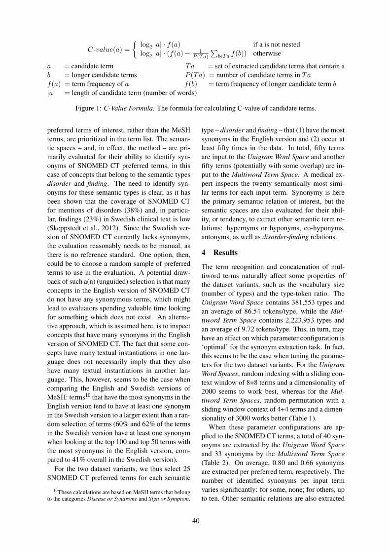
C-value(a) =
{log2 |a| · f(a) if a is not nestedlog2 |a| · (f(a)− 1
P (Ta)
∑bεTa f(b)) otherwise
a = candidate term Ta = set of extracted candidate terms that contain ab = longer candidate terms P (Ta) = number of candidate terms in Taf(a) = term frequency of a f(b) = term frequency of longer candidate term b|a| = length of candidate term (number of words)
Figure 1: C-Value Formula. The formula for calculating C-value of candidate terms.
preferred terms of interest, rather than the MeSHterms, are prioritized in the term list. The seman-tic spaces – and, in effect, the method – are pri-marily evaluated for their ability to identify syn-onyms of SNOMED CT preferred terms, in thiscase of concepts that belong to the semantic typesdisorder and finding. The need to identify syn-onyms for these semantic types is clear, as it hasbeen shown that the coverage of SNOMED CTfor mentions of disorders (38%) and, in particu-lar, findings (23%) in Swedish clinical text is low(Skeppstedt et al., 2012). Since the Swedish ver-sion of SNOMED CT currently lacks synonyms,the evaluation reasonably needs to be manual, asthere is no reference standard. One option, then,could be to choose a random sample of preferredterms to use in the evaluation. A potential draw-back of such a(n) (unguided) selection is that manyconcepts in the English version of SNOMED CTdo not have any synonymous terms, which mightlead to evaluators spending valuable time lookingfor something which does not exist. An alterna-tive approach, which is assumed here, is to inspectconcepts that have many synonyms in the Englishversion of SNOMED CT. The fact that some con-cepts have many textual instantiations in one lan-guage does not necessarily imply that they alsohave many textual instantiations in another lan-guage. This, however, seems to be the case whencomparing the English and Swedish versions ofMeSH: terms10 that have the most synonyms in theEnglish version tend to have at least one synonymin the Swedish version to a larger extent than a ran-dom selection of terms (60% and 62% of the termsin the Swedish version have at least one synonymwhen looking at the top 100 and top 50 terms withthe most synonyms in the English version, com-pared to 41% overall in the Swedish version).
For the two dataset variants, we thus select 25SNOMED CT preferred terms for each semantic
10These calculations are based on MeSH terms that belongto the categories Disease or Syndrome and Sign or Symptom.
type – disorder and finding – that (1) have the mostsynonyms in the English version and (2) occur atleast fifty times in the data. In total, fifty termsare input to the Unigram Word Space and anotherfifty terms (potentially with some overlap) are in-put to the Multiword Term Space. A medical ex-pert inspects the twenty semantically most simi-lar terms for each input term. Synonymy is herethe primary semantic relation of interest, but thesemantic spaces are also evaluated for their abil-ity, or tendency, to extract other semantic term re-lations: hypernyms or hyponyms, co-hyponyms,antonyms, as well as disorder-finding relations.
4 Results
The term recognition and concatenation of mul-tiword terms naturally affect some properties ofthe dataset variants, such as the vocabulary size(number of types) and the type-token ratio. TheUnigram Word Space contains 381,553 types andan average of 86.54 tokens/type, while the Mul-tiword Term Space contains 2,223,953 types andan average of 9.72 tokens/type. This, in turn, mayhave an effect on which parameter configuration is‘optimal’ for the synonym extraction task. In fact,this seems to be the case when tuning the parame-ters for the two dataset variants. For the UnigramWord Spaces, random indexing with a sliding con-text window of 8+8 terms and a dimensionality of2000 seems to work best, whereas for the Mul-tiword Term Spaces, random permutation with asliding window context of 4+4 terms and a dimen-sionality of 3000 works better (Table 1).
When these parameter configurations are ap-plied to the SNOMED CT terms, a total of 40 syn-onyms are extracted by the Unigram Word Spaceand 33 synonyms by the Multiword Term Space(Table 2). On average, 0.80 and 0.66 synonymsare extracted per preferred term, respectively. Thenumber of identified synonyms per input termvaries significantly: for some, none; for others, upto ten. Other semantic relations are also extracted
40
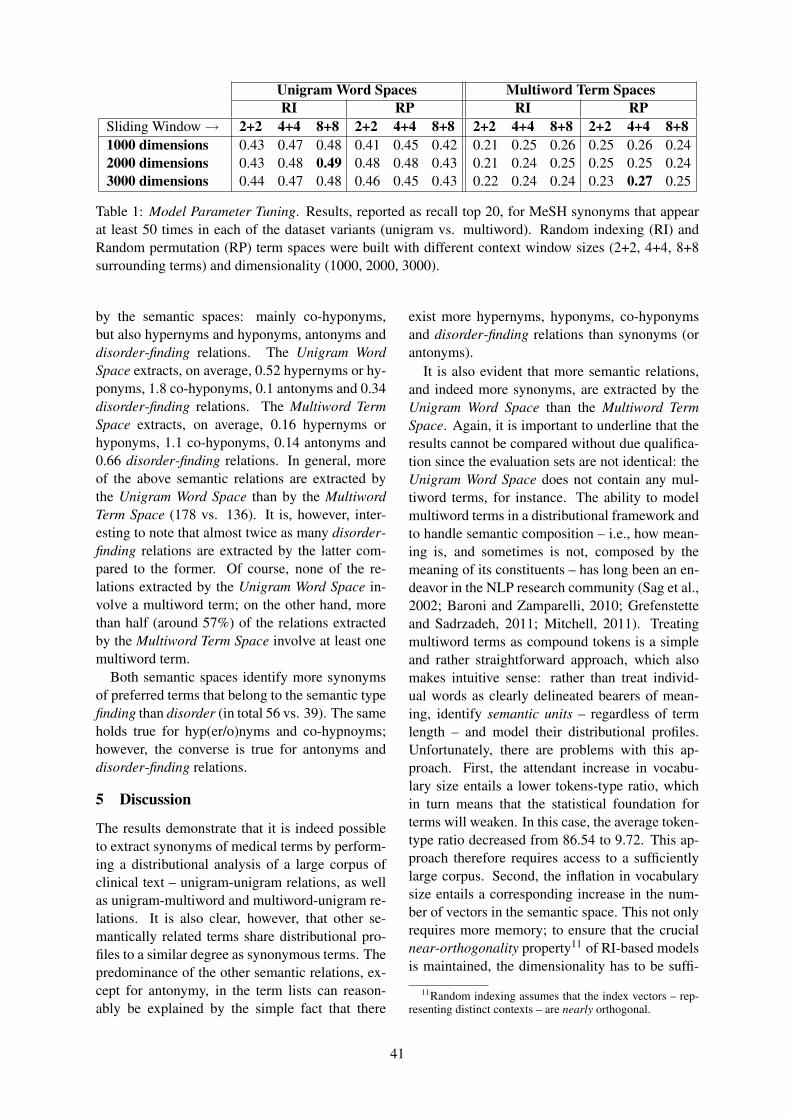
Unigram Word Spaces Multiword Term SpacesRI RP RI RP
Sliding Window→ 2+2 4+4 8+8 2+2 4+4 8+8 2+2 4+4 8+8 2+2 4+4 8+81000 dimensions 0.43 0.47 0.48 0.41 0.45 0.42 0.21 0.25 0.26 0.25 0.26 0.242000 dimensions 0.43 0.48 0.49 0.48 0.48 0.43 0.21 0.24 0.25 0.25 0.25 0.243000 dimensions 0.44 0.47 0.48 0.46 0.45 0.43 0.22 0.24 0.24 0.23 0.27 0.25
Table 1: Model Parameter Tuning. Results, reported as recall top 20, for MeSH synonyms that appearat least 50 times in each of the dataset variants (unigram vs. multiword). Random indexing (RI) andRandom permutation (RP) term spaces were built with different context window sizes (2+2, 4+4, 8+8surrounding terms) and dimensionality (1000, 2000, 3000).
by the semantic spaces: mainly co-hyponyms,but also hypernyms and hyponyms, antonyms anddisorder-finding relations. The Unigram WordSpace extracts, on average, 0.52 hypernyms or hy-ponyms, 1.8 co-hyponyms, 0.1 antonyms and 0.34disorder-finding relations. The Multiword TermSpace extracts, on average, 0.16 hypernyms orhyponyms, 1.1 co-hyponyms, 0.14 antonyms and0.66 disorder-finding relations. In general, moreof the above semantic relations are extracted bythe Unigram Word Space than by the MultiwordTerm Space (178 vs. 136). It is, however, inter-esting to note that almost twice as many disorder-finding relations are extracted by the latter com-pared to the former. Of course, none of the re-lations extracted by the Unigram Word Space in-volve a multiword term; on the other hand, morethan half (around 57%) of the relations extractedby the Multiword Term Space involve at least onemultiword term.
Both semantic spaces identify more synonymsof preferred terms that belong to the semantic typefinding than disorder (in total 56 vs. 39). The sameholds true for hyp(er/o)nyms and co-hypnoyms;however, the converse is true for antonyms anddisorder-finding relations.
5 Discussion
The results demonstrate that it is indeed possibleto extract synonyms of medical terms by perform-ing a distributional analysis of a large corpus ofclinical text – unigram-unigram relations, as wellas unigram-multiword and multiword-unigram re-lations. It is also clear, however, that other se-mantically related terms share distributional pro-files to a similar degree as synonymous terms. Thepredominance of the other semantic relations, ex-cept for antonymy, in the term lists can reason-ably be explained by the simple fact that there
exist more hypernyms, hyponyms, co-hyponymsand disorder-finding relations than synonyms (orantonyms).
It is also evident that more semantic relations,and indeed more synonyms, are extracted by theUnigram Word Space than the Multiword TermSpace. Again, it is important to underline that theresults cannot be compared without due qualifica-tion since the evaluation sets are not identical: theUnigram Word Space does not contain any mul-tiword terms, for instance. The ability to modelmultiword terms in a distributional framework andto handle semantic composition – i.e., how mean-ing is, and sometimes is not, composed by themeaning of its constituents – has long been an en-deavor in the NLP research community (Sag et al.,2002; Baroni and Zamparelli, 2010; Grefenstetteand Sadrzadeh, 2011; Mitchell, 2011). Treatingmultiword terms as compound tokens is a simpleand rather straightforward approach, which alsomakes intuitive sense: rather than treat individ-ual words as clearly delineated bearers of mean-ing, identify semantic units – regardless of termlength – and model their distributional profiles.Unfortunately, there are problems with this ap-proach. First, the attendant increase in vocabu-lary size entails a lower tokens-type ratio, whichin turn means that the statistical foundation forterms will weaken. In this case, the average token-type ratio decreased from 86.54 to 9.72. This ap-proach therefore requires access to a sufficientlylarge corpus. Second, the inflation in vocabularysize entails a corresponding increase in the num-ber of vectors in the semantic space. This not onlyrequires more memory; to ensure that the crucialnear-orthogonality property11 of RI-based modelsis maintained, the dimensionality has to be suffi-
11Random indexing assumes that the index vectors – rep-resenting distinct contexts – are nearly orthogonal.
41
Unigram Word Space Multiword Term SpaceDISORDER FINDING DISORDER FINDING
Synonymssum 18 22 16 17
average 0.72 0.88 0.64 0.68≥ 1 / preferred term 12 12 8 6
involves mwe - - 10 13Hyp(er/o)nyms
sum 12 14 4 4average 0.48 0.56 0.16 0.16
≥ 1 / preferred term 6 8 4 3involves mwe - - 3 3
Co-hyponymssum 34 56 22 33
average 1.36 2.24 0.88 1.32≥ 1 / preferred term 14 17 10 13
involves mwe - - 19 15Antonyms
sum 3 2 4 3average 0.12 0.08 0.16 0.12
≥ 1 / preferred term 3 2 3 3involves mwe - - 0 1
Disorder-Findingsum 11 6 28 5
average 0.44 0.24 1.12 0.2≥ 1 / preferred term 6 5 12 5
involves mwe - - 11 2
Table 2: Evaluation Results. The types of semantic relations extracted among the twenty most se-mantically similar terms of 25 DISORDER and 25 FINDING SNOMED CT preferred terms from eachsemantic space. Sum is the total number of identified relevant terms. Average is the average number ofrelevant terms per preferred term. ≥ 1 / preferred term is the number of preferred terms for which atleast one relevant term is identified. Involves mwe is the number of relevant relations where either thepreferred term or the relevant term is a multiword expression.
ciently large in relation to the number of contexts(represented by index vectors). In the MultiwordTerm Space the vocabulary size is over two million(compared to less than 400,000 in the UnigramWord Space). A dimensionality of 3000 is likelyinsufficient to ensure that each term type has aninitial distinct and uncorrelated representation. Inthe evaluation, there were several examples wheretwo groups of terms – semantically homogenouswithin each group, but semantically heterogenousacross groups – co-existed in the same term list:these ‘topics’ had seemingly collapsed into thesame subspace. Despite these problems, it shouldbe recognized that the Multiword Term Space is, infact, able to retrieve 23 synonymous relations thatinvolve at least one multiword term. The Unigram
Word Space cannot retrieve any such relations.The ability to extract high-quality terms would
seem to be an important prerequisite for this ap-proach to modeling multiword terms in a distribu-tional framework. However, despite employing arather simple means of extracting terms – withoutusing any syntactic information – the terms thatactually appeared in the lists of semantically re-lated terms were mostly reasonable. This perhapsindicates that the term recognition task does notneed to be perfect: terms of interest, of course,need to be identified, but some noise in the formof bad terms might be acceptable. A weaknessof the term recognition part is, however, that toomany terms were identified, which in turn led tothe aforementioned inflation in vocabulary size.
42
Limiting the number of multiword terms in the ini-tial term list – for instance by extracting syntacticphrases as candidate terms – could provide a pos-sible solution to this problem.
Overall, more synonyms were identified for thesemantic type finding than for disorder. One pos-sible explanation for this could be that there aremore ways of describing a finding than a disorder– not all semantic types can be assumed to havethe same number of synonyms. The same holdstrue for all other semantic relations except for dis-order-finding, where disorders generated a muchlarger number of distributionally similar findingsthan vice versa. This could perhaps also be ex-plained by the possible higher number of syn-onyms for finding than disorder.
When this method was evaluated using theEnglish version of SNOMED CT, 16-24% ofknown synonyms were identified (Henriksson etal., 2013). In this case, however, we extractedsynonym candidates for terms that may or maynot have synonyms. This is thus a scenario thatmore closely resembles how this method wouldactually be used in a real-life setting to populatea terminology with synonyms. Although the com-parison with MeSH showed that terms with manysynonyms in English also tend to have at least onesynonym in Swedish, approximately 40% of themdid not have any synonyms. It is thus not certainthat the terms used in this evaluation all have atleast one synonym, which was also noted by theevaluator in this study.
6 Conclusions
In this study, we have demonstrated a methodthat could potentially be used to expedite the lan-guage porting process of terminologies such asSNOMED CT. With access to a large corpus ofclinical text in the target language and an initialset of terms, this language-independent method isable to extract and present candidate synonyms tothe lexicographer, thereby providing valuable sup-port for semi-automatic terminology development.A means to model multiword terms in a distri-butional framework is an important feature of themethod and is crucial for the synonym extractiontask.
Acknowledgments
This work was partly supported by the SwedishFoundation for Strategic Research through the
project High-Performance Data Mining for DrugEffect Detection (ref. no. IIS11-0053) at Stock-holm University, Sweden, and partly funded bythe Stockholm University Academic Initiativethrough the Interlock project. Finally, we wouldlike to thank the reviewers for their constructivefeedback.
ReferencesIon Androutsopoulos and Prodromos Malakasiotis.
2010. A Survey of Paraphrasing and Textual En-tailment Methods. Journal of Artificial IntelligenceResearch, 38:135–187.
Satanjeev Banerjee and Ted Pedersen. 2003. The De-sign, Implementation, and Use of the Ngram Statis-tic Package. In Proceedings of CICLing, pages 370–381.
Marco Baroni and Roberto Zamparelli. 2010. Nounsare Vectors, Adjectives are Matrices: RepresentingAdjective-Noun Constructions in Semantic Space.In Proceedings of EMNLP, pages 1183–1193.
Vincent D. Blondel, Anahı Gajardo, Maureen Hey-mans, Pierre Senellart, and Paul Van Dooren.2004. A Measure of Similarity between Graph Ver-tices: Applications to Synonym Extraction and WebSearching. SIAM Review, 46(4):647–666.
Aaron M. Cohen and William R. Hersh. 2005. A Sur-vey of Current Work in Biomedical Text Mining.Briefings in Bioinformatics, 6(1):57–71.
Trevor Cohen and Dominic Widdows. 2009. EmpiricalDistributional Semantics: Methods and BiomedicalApplications. J Biomed Inform, 42(2):390–405.
AM Cohen, WR Hersh, C Dubay, and K Spackman.2005. Using co-occurrence network structure toextract synonymous gene and protein names frommedline abstracts. BMC Bioinformatics, 6(1):103.
Mike Conway and Wendy W. Chapman. 2012. Dis-covering Lexical Instantiations of Clinical Con-cepts using Web Services, WordNet and Corpus Re-sources. In AMIA Fall Symposium, page 1604.
Hercules Dalianis, Martin Hassel, and SumithraVelupillai. 2009. The Stockholm EPR Corpus:Characteristics and Some Initial Findings. In Pro-ceedings of ISHIMR, pages 243–249.
Scott Deerwester, Susan T. Dumais, George W Fur-nas, Thomas K Landauer, and Richard Harshman.1990. Indexing by Latent Semantic Analysis. Jour-nal of the American Society for Information Science,41(6):391–407.
Susan T. Dumais and Thomas K. Landauer. 1997. ASolution to Plato’s Problem: The Latent Semantic
43
Analysis Theory of Acquisition, Induction and Rep-resentation of Knowledge. Psychological Review,104(2):211–240.
Katerina Frantzi and Sophia Ananiadou. 1996. Ex-tracting Nested Collocations. In Proceedings ofCOLING, pages 41–46.
Katerina Frantzi, Sophia Ananiadou, and HidekiMima. 2000. Automatic Recognition of Multi-Word Terms: The C-value/NC-value Method. In-ternational Journal on Digital Libraries, 3(2):115–130.
Edward Grefenstette and Mehrnoosh Sadrzadeh. 2011.Experimental Support for a Categorical Composi-tional Distributional Model of Meaning. In Pro-ceedings of EMNLP, pages 1394–1404.
Zellig S. Harris. 1954. Distributional Structure. Word,10:146–162.
Marti Hearst. 1992. Automatic Acquisition of Hy-ponyms from Large Text Corpora. In Proceedingsof COLING, pages 539–545.
Aron Henriksson and Martin Hassel. 2013. Optimiz-ing the Dimensionality of Clinical Term Spaces forImproved Diagnosis Coding Support. In Proceed-ings of Louhi.
Aron Henriksson, Hans Moen, Maria Skeppstedt, Ann-Marie Eklund, and Vidas Daudaravicius. 2012.Synonym Extraction of Medical Terms from Clini-cal Text Using Combinations of Word Space Mod-els. In Proceedings of SMBM, pages 10–17.
Aron Henriksson, Mike Conway, Martin Duneld, andWendy W. Chapman. 2013. Identifying Syn-onymy between SNOMED Clinical Terms of Vary-ing Length Using Distributional Analysis of Elec-tronic Health Records. In AMIA Annual Symposium(submitted).
Donald Hindle. 1990. Noun Classification fromPredicate-Argument Structures. In Proceedings ofACL, pages 268–275.
Pentti Kanerva, Jan Kristofersson, and Anders Holst.2000. Random Indexing of Text Samples for LatentSemantic Analysis. In Proceedings CogSci, page1036.
John McCrae and Nigel Collier. 2008. SynonymSet Extraction from the Biomedical Literature byLexical Pattern Discovery. BMC Bioinformatics,9(1):159.
Stephane M. Meystre, Guergana K. Savova, Karin C.Kipper-Schuler, John F. Hurdle, et al. 2008. Ex-tracting Information from Textual Documents in theElectronic Health Record: A Review of Recent Re-search. Yearb Med Inform, 35:128–44.
Jeffrey Mitchell. 2011. Composition in DistributionalModels of Semantics. Ph.D. thesis, University ofEdinburgh.
Kotaro Nakayama, Takahiro Hara, and Shojiro Nishio.2007. Wikipedia Mining for an Association WebThesaurus Construction. In Proceedings of WISE,pages 322–334.
Alexander Panchenko. 2013. Similarity Measures forSemantic Relation Extraction. Ph.D. thesis, PhDthesis, Universite catholique de Louvain & BaumanMoscow State Technical University.
Yves Peirsman and Dirk Geeraerts. 2009. PredictingStrong Associations on the Basis of Corpus Data. InProceedings of EACL, pages 648–656.
Ivan A. Sag, Timothy Baldwin, Francis Bond, AnnCopestake, and Dan Flickinger. 2002. MultiwordExpressions: A Pain in the Neck for NLP. In Pro-ceedings of CICLing, pages 1–15.
Magnus Sahlgren, Anders Holst, and Pentti Kanerva.2008. Permutations as a Means to Encode Orderin Word Space. In Proceedings of CogSci, pages1300–1305.
Magnus Sahlgren. 2006. The Word-Space Model:Using Distributional Analysis to Represent Syntag-matic and Paradigmatic Relations between Words inHigh-Dimensional Vector Spaces. Ph.D. thesis, PhDthesis, Stockholm University.
Maria Skeppstedt, Maria Kvist, and Hercules Dalianis.2012. Rule-based Entity Recognition and Coverageof SNOMED CT in Swedish Clinical Text. In Pro-ceedings of LREC, pages 1250–1257.
Lonneke van der Plas and Jorg Tiedemann. 2006.Finding Synonyms Using Automatic Word Align-ment and Measures of Distributional Similarity. InProceedings of COLING/ACL, pages 866–873.
Hua Wu and Ming Zhou. 2003. Optimizing Syn-onym Extraction Using Monolingual and BilingualResources. In Proceedings of the Second Interna-tional Workshop on Paraphrasing, pages 72–79.
Hong Yu and Eugene Agichtein. 2003. ExtractingSynonymous Gene and Protein Terms from Biolog-ical Literature. Bioinformatics, 19(suppl 1):i340–i349.
Qing T Zeng, Doug Redd, Thomas Rindflesch, andJonathan Nebeker. 2012. Synonym, Topic Modeland Predicate-Based Query Expansion for Retriev-ing Clinical Documents. In Proceedings AMIA An-nual Symposium, pages 1050–9.
Ziqi Zhang, Jose Iria, Christopher Brewster, and FabioCiravegna. 2008. A Comparative Evaluation ofTerm Recognition Algorithms. In Proceedings ofLREC.
44
Proceedings of the 2013 Workshop on Biomedical Natural Language Processing (BioNLP 2013), pages 45–53,Sofia, Bulgaria, August 4-9 2013. c©2013 Association for Computational Linguistics
Unsupervised Linguistically-Driven Reliable Dependency ParsesDetection and Self-Training for Adaptation to the Biomedical Domain
Felice Dell’Orletta, Giulia Venturi, Simonetta Montemagni
Istituto di Linguistica Computazionale “Antonio Zampolli” (ILC–CNR)
Via G. Moruzzi, 1 – Pisa (Italy)
{felice.dellorletta,giulia.venturi,simonetta.montemagni}@ilc.cnr.it
Abstract
In this paper, a new self–training method
for domain adaptation is illustrated, where
the selection of reliable parses is car-
ried out by an unsupervised linguistically–
driven algorithm, ULISSE. The method
has been tested on biomedical texts with
results showing a significant improve-
ment with respect to considered baselines,
which demonstrates its ability to capture
both reliability of parses and domain–
specificity of linguistic constructions.
1 Introduction
As firstly demonstrated by (Gildea, 2001), pars-
ing systems have a drop of accuracy when tested
against domain corpora outside of the data from
which they were trained. This is a real prob-
lem in the biomedical domain where, due to the
rapidly expanding body of biomedical literature,
the need for increasingly sophisticated and effi-
cient biomedical text mining systems is becom-
ing more and more pressing. In particular, the ex-
istence of natural language parsers reliably deal-
ing with biomedical texts represents the prerequi-
ste for identifying and extracting knowledge em-
bedded in them. Over the last years, this prob-
lem has been tackled within the biomedical NLP
community from different perspectives. The de-
velopment of a domain–specific annotated corpus,
i.e. the Genia Treebank (Tateisi, Yakushiji, Ohta,
& Tsujii, 2005), played a key role by providing a
sound basis for empirical performance evaluation
as well as training of parsers. On the other hand,
several attempts have been made to adapt general
parsers to the biomedical domain. First experi-
ments in this direction are reported in (Clegg &
Shepherd, 2005) who first compared the perfor-
mance of three different parsers against the Ge-
nia treebank and a sample of the Penn Treebank
(PTB) (Mitchell P. Marcus & Santorini, 1993) in
order to carry out an inter–domain analysis of
the typology of errors made by each parser and
demonstrated that by integrating the output of the
three parsers they achieved statistically significant
performance gains. Three different methods of
parser adaptation for the biomedical domain have
been proposed by (Lease & Charniak, 2005) who,
starting from the results of unknown word rate
experiments carried out on the Genia treebank,
adapted a PTB–trained parser by improving the
Part–Of–Speech tagging accuracy and by relying
on an external domain–specific lexicon. More re-
cently, (McClosky, Charniak, & Johnson, 2010)
and (Plank & van Noord, 2011) devised adaptation
methods based on domain similarity measures. In
particular, both of them adopted lexical similar-
ity measures to automatically select from an anno-
tated collection of texts those training data which
is more relevant, i.e. lexically closer, to adapt the
parser to the target domain.
A variety of semi–supervised approaches,
where unlabeled data is used in addition to labeled
training data, have been recently proposed in the
literature in order to adapt parsing systems to new
domains. Among these approaches, the last few
years have seen a growing interest in self–training
for domain adaptation, i.e. a method for using au-
tomatically annotated data from a target domain
when training supervised models. Self–training
methods proposed so far mainly differ at the level
of the selection of parse trees to be added to the
in–domain gold trees as further training data. De-
pending on whether or not external supervised
classifiers are used to select the parses to be added
to the gold–training set, two types of methods are
envisaged in the literature. The first is the case,
among others, of: (Kawahara & Uchimoto, 2008),
using a machine learning classifier to predict the
reliability of parses on the basis of different fea-
ture types; or (Sagae & Tsujii, 2007), selecting
45
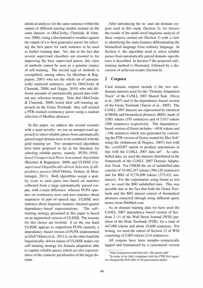
identical analyses for the same sentence within the
output of different parsing models trained on the
same dataset; or (McClosky, Charniak, & John-
son, 2006), using a discriminative reranker against
the output of a n–best generative parser for select-
ing the best parse for each sentence to be used
as further training data. Yet, due to the fact that
several supervised classifiers are resorted to for
improving the base supervised parser, this class
of methods cannot be seen as a genuine istance
of self–training. The second type of methods is
exemplified, among others, by (Reichart & Rap-
poport, 2007) who use the whole set of automat-
ically analyzed sentences, and by (McClosky &
Charniak, 2008) and (Sagae, 2010) who add dif-
ferent amounts of automatically parsed data with-
out any selection strategy. Note that (McClosky
& Charniak, 2008) tested their self–training ap-
proach on the Genia Treebank: they self–trained
a PTB–trained costituency parser using a random
selection of Medline abstracts.
In this paper, we address the second scenario
with a main novelty: we use an unsupervised ap-
proach to select reliable parses from automatically
parsed target domain texts to be combined with the
gold–training set. Two unsupervised algorithms
have been proposed so far in the literature for
selecting reliable parses, namely: PUPA (POS–
based Unsupervised Parse Assessment Algorithm)
(Reichart & Rappoport, 2009) and ULISSE (Un-
supervised LInguiStically–driven Selection of dE-
pendency parses) (Dell’Orletta, Venturi, & Mon-
temagni, 2011). Both algorithms assign a qual-
ity score to each parse tree based on statistics
collected from a large automatically parsed cor-
pus, with a main difference: whereas PUPA oper-
ates on costituency trees and uses statistics about
sequences of part–of–speech tags, ULISSE uses
statistics about linguistic features checked against
dependency–based representations. The self–
training strategy presented in this paper is based
on an augmented version of ULISSE. The reasons
for this choice are twofold: if on the one hand
ULISSE appears to outperform PUPA (namely, a
dependency–based version of PUPA implemented
in (Dell’Orletta et al., 2011)), on the other hand the
linguistically–driven nature of ULISSE makes our
self–training strategy for domain adaptation able
to capture reliable parses which are also represen-
tative of the syntactic peculiarities of the target do-
main.
After introducing the in– and out–domain cor-
pora used in this study (Section 2), we discuss
the results of the multi–level linguistic analysis of
these corpora carried out (Section 3) with a view
to identifying the main features differentiating the
biomedical language from ordinary language. In
Section 4, the algorithm used to select reliable
parses from automatically parsed domain–specific
texts is described. In Section 5 the proposed self–
training method is illustrated, followed by a dis-
cussion of achieved results (Section 6).
2 Corpora
Used domain corpora include i) the two out–
domain datasets used for the “Domain Adaptation
Track” of the CoNLL 2007 Shared Task (Nivre
et al., 2007) and ii) the dependency–based version
of the Genia Treebank (Tateisi et al., 2005). The
CoNLL 2007 datasets are represented by chemical
(CHEM) and biomedical abstracts (BIO), made of
5,001 tokens (195 sentences) and of 5,017 tokens
(200 sentences) respectively. The dependency–
based version of Genia includes∼493k tokens and
∼18k sentences which was generated by convert-
ing the PTB version of Genia created by Illes Solt1
using the (Johansson & Nugues, 2007) tool with
the -conll2007 option to produce annotations in
line with the CoNLL 2007 data set2. As unla-
belled data, we used the datasets distributed in the
framework of the CoNLL 2007 Domain Adapta-
tion Track. For CHEM the set of unlabelled data
consists of 10,482,247 tokens (396,128 sentences)
and for BIO of 9,776,890 tokens (375,421 sen-
tences). For the experiments using Genia as test
set, we used the BIO unlabelled data. This was
possible due to the fact that both the Genia Tree-
bank and the BIO dataset consist of biomedical
abstracts extracted (though using different query
terms) from PubMed.com.
As in–domain training data we have used the
CoNLL 2007 dependency–based version of Sec-
tions 2–11 of the Wall Street Journal (WSJ) par-
tition of the Penn Treebank (PTB), for a total of
447,000 tokens and about 18,600 sentences. For
testing, we used the subset of Section 23 of WSJ
consisting of 5,003 tokens (214 sentences).
All corpora have been morpho–syntactically
tagged and lemmatized by a customized version
1http://categorizer.tmit.bme.hu/∼illes/genia ptb/2In order to be fully compliant with the PTB PoS tagset,
we changed the PoS label of all punctuation marks.
46
of the pos–tagger described in (Dell’Orletta, n.d.)
and dependency parsed by the DeSR parser us-
ing Multi–Layer Perceptron (MLP) as learning al-
gorithm (Attardi, Dell’Orletta, Simi, & Turian,
n.d.), a state–of–the–art linear–time Shift–Reduce
dependency parser following a “stepwise” ap-
proach (Buchholz & Marsi, 2006).
3 Linguistic analysis of biomedical
abstrats vs newspaper articles
For the specific concerns of this study, we carried
out a comparative linguistic analysis of four dif-
ferent corpora, taken as representative of ordinary
language and biomedical language. In each case,
we took into account a gold (i.e. manually an-
notated) corpus, and an unlabelled corpus, which
was automatically annotated. By comparing the
results obtained with respect to gold and automat-
ically annotated texts, we intend to demonstrate
the reliability of features extracted from automat-
ically annotated texts. As data representative of
ordinary language we took i) the whole WSJ sec-
tion of the Penn Treebank3 including 39,285,425
tokens (1,625,606 sentences) and ii) the sections
2–11 of the WSJ. For what concerns the biomed-
ical domain, we relied on the Genia Treebank in
order to guarantee comparability of the results of
our linguistic analysis with previous studies car-
ried out on this reference corpus. As automatically
annotated data we used the corpus of biomedical
abstract (BIO) distributed as out–domain dataset
used for the “Domain Adaptation Track” of the
CoNLL 2007 Shared Task.
In order to get evidence of the differences hold-
ing between the WSJ newspaper articles and the
selected biomedical abstracts, the four corpora
have been compared with respect to a wide typol-
ogy of features (i.e. raw text, lexical, morpho–
syntactic and syntactic). Let us start from raw
text features, in particular from average sen-
tence length (calculated as the average number
of words per sentence): as Figure 1 shows, both
the corpus of automatically parsed newspaper ar-
ticles (WSJ unlab) and the manually annotated
one (WSJ gold) contain shorter sentences with re-
spect to both the automatically parsed biomedi-
cal abstrats (BIO unlab) and the manually anno-
tated ones (Genia gold), a result which is in line
3This corpus represents to the unlabelled data set dis-tributed for the CoNLL 2007 Shared Task on DependencyParsing, domain adaptation track.
Figure 1: Average sentence length in biomedical
and newspaper corpora.
with (Clegg & Shepherd, 2005) findings. When
we focus on the lexical level, BIO unlab and
Genia gold appear to have quite a similar per-
centage of lexical items which is not contained
in WSJ gold (23.13% and 26.14% respectively)
while the out–of–vocabulary rate of WSJ unlab
is much lower, i.e. 8.69%. Similar results were
recorded by (Lease & Charniak, 2005) who report
the unknown word rate for various genres of tec-
nical literature.
Let us focus now on the morpho–syntactic level.
If we consider the distribution of nouns, verbs
and adjectives, three features typically represent-
ing stylistic markers associated with different lin-
guistic varieties (Biber & Conrad, 2009), it can
be noticed (see Figures 2(a) and 2(c)) that the
biomedical abstracts contain a higher percentage
of nouns and adjectives while showing a signif-
icantly lower percentage of verbs (Figure 2(b)).
The syntactic counterpart of the different distri-
bution of morpho–syntactic categories can be ob-
served in Table 1, reporting the percentage distri-
bution of the first ten Parts–of–Speech dependency
triplets occurring in the biomedical and newspaper
corpora: each triplet is described as the sequence
of the PoS of a dependent and a head linked by a
depedency arc, by also considering the PoS of the
head father. It turned out that biomedical abstracts
are characterized by nominal dependency triplets,
e.g. two nouns and a preposition (NN–NN–IN)
or noun, preposition, noun (NN–IN–NN) or ad-
jective, noun and preposition (JJ–NN–IN), which
occur more frequently than verbal triplets, such
as determiner, noun and verb (DT–NN–VBZ) or a
verbal root (.–VBD–ROOT)4. Interestingly, in Ge-
nia gold no verbal triplet occurs within the top ten
triplets, which cover the 21% of the total amount
4We named ‘ROOT’ the artificial root node.
47
(a) Distribution of Nouns (b) Distribution of Verbs (c) Distribution of Adjectives
Figure 2: Distribution of some Parts–of–Speech in biomedical and newspaper corpora.
of triplets occurring in the corpus. By contrast,
the same top ten triplets represent only ∼11% in
WSJ gold, testifying the wider variety of syntac-
tic constructions occurring in newspaper articles
with respect to texts of the biomedical domain.
This is also proved by the total amount of differ-
ent PoS dependency triplets occurring in the two
gold datasets, i.e. 7,827 in WSJ gold and 5,064
in Genia gold even though the Genia Treebank is
∼50,000–tokens bigger.
Further differences can be observed at a deeper
syntactic level of analysis. This is the case of the
average depth of embedded complement ‘chains’
governed by a nominal head. Figure 3(a) shows
that biomedical abstracts are characterized by an
average depth which is higher than the one ob-
served in newspaper articles. A similar trend
can be observed for what concerns the distribu-
tion of ‘chains’ by depth. In Figure 3(b) shows
that WSJ unlab and WSJ gold ‘chains’, on the one
hand, and BIO unlab and Genia gold ‘chains’,
on the other hand, overlap. The corpora have
also been compared with respect to i) the av-
erage length of dependency links, measured in
terms of the words occurring between the syntac-
tic head and the dependent (excluding punctua-
tion marks), and ii) the average depth of the whole
parse tree, calculated in terms of the longest path
from the root of the dependency tree to a leaf. In
both cases it can be noted that i) the biomedical
abstracts contain much longer dependency links
than newswire texts (Figure 3(c)) and ii) the av-
erage depth of BIO unlab and Genia gold parse
trees is higher than in the case of the WSJ unlab
and WSJ gold (Figure 3(d)). A further distin-
guishing feature of the biomedical abstracts con-
cerns the average depth of ‘chains’ of embed-
ded subordinate clauses, calculated here by taking
into account both clausal arguments and comple-
ments linked to a verbal sentence root. As Figure
3(e) shows, both BIO unlab and Genia gold have
shorter ‘chains’ with respect to the ones contained
in the newspaper articles. Interestingly, a careful
analysis of the distributions by depth of ‘chains’
of embedded subordinate clauses shows that the
biomedical abstracts appear to have i) a higher oc-
currence of ‘chains’ including just one subordinate
clause and ii) a lower percentage of deep ‘chains’
with respect to newswire texts. Finally, we com-
pared the two types of corpora with respect to the
distribution of verbal roots. The biomedical ab-
stracts resulted to be characterised by a lower per-
centage of verbal roots with respect to newspaper
articles (see Figure 3(f)). This is in line with the
distribution of verbs as well as of the nominal de-
pendency triplets observed in the biomedical ab-
stracts at the morpho–syntactic level of analysis.
Interestingly, the results obtained with respect
to automatically parsed and manually annotated
data show similar trends for both considered in–
and out–domain corpora, thus demonstrating the
reliability of features monitored against automat-
ically annotated data. In what follows, we will
show how detected linguistic peculiarities can be
exploited in a domain adaptation scenario.
4 Linguistically–driven Unsupervised
Ranking of Parses for Self–training
In the self–training approach illustrated in this pa-
per, the selection of parses from the automatically
annotated target domain dataset is guided by an
augmented version of ULISSE, an unsupervised
linguistically–driven algorithm to select reliable
parses from the output of dependency annotated
texts (Dell’Orletta et al., 2011) which has shown
a good performance for two different languages
48
WSJ gold WSJ unlab Genia gold BIO unlab
Triplet % Freq Triplet % Freq Triplet % Freq Triplet % Freq
DT-NN-IN 2.03 DT-NN-IN 1.72 NN-NN-IN 3.66 DT-NN-IN 2.87
.-VBD-ROOT 1.61 .-VBD-ROOT 1.30 NN-IN-NN 2.93 NN-IN-NN 2.39
NN-IN-NN 1.11 JJ-NN-IN 0.99 DT-NN-IN 2.48 JJ-NN-IN 2.08
JJ-NN-IN 1.10 NN-IN-NN 0.97 JJ-NN-IN 1.96 NN-NN-IN 1.73
.-VBZ-ROOT 1.09 NNP-NNP-IN 0.87 NN-NNS-IN 1.88 IN-NN-IN 1.72
NNP-NNP-IN 0.95 DT-NN-VBD 0.85 JJ-NNS-IN 1.77 JJ-NNS-IN 1.36
DT-NN-VBZ 0.89 NN-VBD-ROOT 0.80 IN-NN-IN 1.65 .-VBD-ROOT 1.33
DT-NN-VBD 0.87 JJ-NNS-IN 0.79 NN-CC-IN 1.64 NNS-IN-NN 1.13
JJ-NNS-IN 0.87 NNP-NNP-VBD 0.78 NNS-IN-NN 1.56 NNP-NN-IN 1.03
IN-NN-IN 0.87 .-VBZ-ROOT 0.75 NN-NN-CC 1.47 NN-IN-VBN 0.93
Table 1: Frequency distribution of the first ten Parts–of–Speech dependency triplets in biomedical and
newspaper corpora.
(a) Depth of embedded complement‘chains’
(b) Distribution of embedded com-plement ‘chains’ by depth
(c) Length of dependency links
(d) Parse tree depth (e) Depth of embedded subordinateclauses ‘chains’
(f) Distribution of verbal roots
Figure 3: Syntactic features in biomedical and newspaper corpora.
(English and Italian) against the output of two su-
pervised parsers (MST, (McDonald, Lerman, &
Pereira, 2006) and DeSR, (Attardi, 2006)) se-
lected for their behavioral differences (McDonald
& Nivre, 2007). ULISSE assigns to each depen-
dency tree a score quantifying its reliability based
on a wide range of linguistic features. After col-
lecting statistics about selected features from a
corpus of automatically parsed sentences, for each
newly parsed sentence ULISSE computes a relia-
bility score using the previously extracted feature
statistics. In its reliability assessment, ULISSE ex-
ploits both global and local features, where global
features (listed in Table 2 and discussed in Sec-
tion 3) are computed with respect to each sen-
tence and averaged over all sentences in the cor-
pus, and the local features with respect to indi-
vidual dependency links and averaged over all of
them. Local features include the plausibility of
a dependency link calculated by considering se-
lected features of the dependent and its govern-
ing head as well as of the head father: whereas
in ULISSE the selected features were circum-
scribed to part–of–speech information (so–called
“ArcPOSFeat” feature), in this version of the al-
gorithm a new local feature has been introduced,
named “ArcLemmaFeat”, which exploits lemma
information. “ArcPOSFeat” is able to capture the
different distribution of PoS dependency triplets
(see Table 1), along with the type of dependency
link, while the newly introduced “ArcLemmaFeat”
is meant to capture the lexical peculiarities of the
target domain (see Section 3). As demonstrated
in (Dell’Orletta et al., 2011), both global and lo-
49
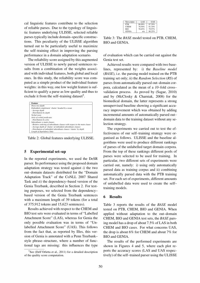
cal linguistic features contribute to the selection
of reliable parses. Due to the typology of linguis-
tic features underlying ULISSE, selected reliable
parses typically include domain–specific construc-
tions. This peculiarity of the ULISSE algorithm
turned out to be particularly useful to maximize
the self–training effect in improving the parsing
performance in a domain adaptation scenario.
The reliability score assigned by this augmented
version of ULISSE to newly parsed sentences re-
sults from a combination of the weights associ-
ated with individual features, both global and local
ones. In this study, the reliability score was com-
puted as a simple product of the individual feature
weights: in this way, one low weight feature is suf-
ficient to qualify a parse as low quality and thus to
exclude it from the self–training dataset5.
Feature
Parse tree depth
Embedded complement ‘chains’ headed by a noun
- Average depth
- Distribution by depth
Verbal roots
Arity of verbal predicates
- Distribution by arity
Subordinate vs main clauses
- Relative ordering of subordinate clauses with respect to the main clause
- Average depth of ‘chains’ of embedded subordinate clauses
- Distribution of embedded subordinate clauses ‘chains’ by depth
Length of dependency links
Table 2: Global features underlying ULISSE.
5 Experimental set–up
In the reported experiments, we used the DeSR
parser. Its performance using the proposed domain
adaptation strategy was tested against i) the two
out–domain datasets distributed for the “Domain
Adaptation Track” of the CoNLL 2007 Shared
Task and ii) the dependency–based version of the
Genia Treebank, described in Section 2. For test-
ing purposes, we selected from the dependency–
based version of the Genia Treebank sentences
with a maximum length of 39 tokens (for a total
of 375,912 tokens and 15,623 sentences).
Results achieved with respect to the CHEM and
BIO test sets were evaluated in terms of “Labelled
Attachment Score” (LAS), whereas for Genia the
only possible evaluation was in terms of “Un-
labelled Attachment Score” (UAS). This follows
from the fact that, as reported by Illes, this ver-
sion of Genia is annotated with a Penn Treebank–
style phrase–structure, where a number of func-
tional tags are missing: this influences the type
5See (Dell’Orletta et al., 2011) for a detailed descriptionof the quality score computation.
Test corpus LAS UAS
PTB 86.09% 87.29%
CHEM 78.50% 81.10%
BIO 78.65% 79.97%
GENIA n/a 80.25%
Table 3: The BASE model tested on PTB, CHEM,
BIO and GENIA.
of evaluation which can be carried out against the
Genia test set.
Achieved results were compared with two base-
lines, represented by: i) the Baseline model
(BASE), i.e. the parsing model trained on the PTB
training set only; ii) the Random Selection (RS) of
parses from automatically parsed out–domain cor-
pora, calculated as the mean of a 10–fold cross–
validation process. As proved by (Sagae, 2010)
and by (McClosky & Charniak, 2008) for the
biomedical domain, the latter represents a strong
unsupervised baseline showing a significant accu-
racy improvement which was obtained by adding
incremental amounts of automatically parsed out–
domain data to the training dataset without any se-
lection strategy.
The experiments we carried out to test the ef-
fectiveness of our self–training strategy were or-
ganised as follows. ULISSE and the baseline al-
gorithms were used to produce different rankings
of parses of the unlabelled target domain corpora.
From the top of these rankings different pools of
parses were selected to be used for training. In
particular, two different sets of experiments were
carried out, namely: i) using only automatically
parsed data as training corpus and ii) combining
automatically parsed data with the PTB training
set. For each set of experiments, different amounts
of unlabelled data were used to create the self–
training models.
6 Results
Table 3 reports the results of the BASE model
tested on PTB, CHEM, BIO and GENIA. When
applied without adaptation to the out–domain
CHEM, BIO and GENIA test sets, the BASE pars-
ing model has a drop of about 7.5% of LAS in both
CHEM and BIO cases. For what concerns UAS,
the drop is about 6% for CHEM and about 7% for
BIO and GENIA.
The results of the performed experiments are
shown in Figures 4 and 5, where each plot re-
ports the accuracy scores (LAS and UAS respec-
tively) of the self–trained parser using the ULISSE
50
(a) LAS for CHEM without PTB training set. (b) LAS for BIO without the PTB training set.
(c) LAS for CHEM with the PTB training set. (d) LAS for BIO with the PTB training set.
Figure 4: LAS of the different self–training models in the two sets of performed experiments.
(a) UAS for GENIA without the PTB training set. (b) UAS for GENIA with the PTB training set.
Figure 5: UAS of the different self–training models for GENIA.
algorithm (henceforth, ULISSE–Stp) and of the
baseline models (RS and BASE). The parser ac-
curacy was computed with respect to different
amounts of automatically parsed data which were
used to create the self–trained parsing model. For
this purpose, we considered six different pools of
250k, 450k, 900k, 1000k, 1350k and 1500k to-
kens. Plots are organized by experiment type: i.e.
the results in subfigures 4(a), 4(b) and 5(a) are
achieved by using only automatically parsed data
as training corpus, whereas those reported in the
other subfigures refer to models trained on auto-
matically parsed data combined with PTB. Note
that in all figures the line named best–RS repre-
sents the best RS score for each pool of k tokens in
the 10–fold cross–validation process.
For what concerns BIO and CHEM, in the first
set of experiments ULISSE–Stp turned out to be
the best self–training algorithm: this is always the
case for CHEM (see subfigure 4(a)), whereas for
BIO (see subfigure 4(b)) it outperforms all base-
lines only when pools of tokens >= 900k are
added. When 900k tokens are used, ULISSE–Stp
allows a LAS improvement of 0.81% on CHEM
and of 0.61% on BIO with respect to RS, and
of 0.62% on CHEM and of 0.48% on BIO with
respect to BASE. It is interesting to note that
ULISSE–Stp using only automatically parsed data
for training achieves better results than BASE (us-
ing the PTB gold training set): to our knowledge,
a similar result has never been reported in the lit-
erature. The behaviour is similar also when the
51
experiments are evaluated in terms of UAS6.
The results achieved in the first set of experi-
ments carried out on the GENIA test set (see 5(a))
differ significantly from what we observed for
CHEM and BIO: in this case, the BASE model ap-
pears to outperform all the other algorithms, with
the ULISSE–Stp algorithm being however more
effective than the RS baselines.
Figures 4(c), 4(d) and 5(b) report the results of
the second set of experiments, i.e. those carried
out by also including PTB in the training set. Note
that in these plots the RS+PTB lines represent the
score of the parser models trained on the pools
of tokens used to obtain the best–RS line com-
bined with the PTB gold training set. It can be
observed that the ULISSE–Stp+PTB self–training
model outperforms all baselines for CHEM, BIO
and GENIA for all the different sizes of pools of
selected tokens. For each pool of parsed data, Ta-
ble 4 records the improvement and the error reduc-
tion observed with respect to the BASE model.
Pool of tokens CHEM Err. red. BIO Err. red. GENIA Err. red.
250k 0.8 3.72 0.76 3.55 0.97 4.91
450k 1.1 5.12 0.54 2.53 1.52 7.7
900k 1.14 5.3 1.02 4.77 1.31 6.63
1000k 0.8 3.72 1.56 7.29 1.2 6.08
1350k 0.4 1.49 1.46 6.82 0.94 4.76
1500k 0.78 3.62 0.75 3.37 0.66 3.34
Table 4: % improvement of ULISSE–Stp+PTB vs
BASE reported in terms of LAS for CHEM and
BIO and of UAS for GENIA.
Differently from (Sagae, 2010) (with a
constituency–based parser), in this set of experi-
ments the self–training approach based on random
selection of sentences (i.e. the best–RS+PTB
baseline) doesn’t achieve any improvement with
respect to the BASE model with only minor
exceptions (observed e.g. with 250k and 450k
pools of added tokens for CHEM and with 250k
for GENIA). Moreover, even when the best–RS
LAS is higher than the ULISSE–Stp score (e.g.
in the first pools of k of Figure 4(b)), ULISSE–
Stp+PTB turns out to be more effective than
the best–RS+PTB baseline (Figure 4(d)). These
results may follow from the fact that ULISSE–Stp
is able to capture not only reliable parses but also,
and more significantly here, parses which reflect
the syntactic peculiarities of the target domain.
Table 5 shows the results of the different
ULISSE–Stp+PTB models tested on the PTB test
6In this paper, for CHEM and BIO experiments we reportonly the LAS scores since this is the standard evaluation met-ric for dependency parsing.
set: no LAS improvement is observed with respect
to the results obtained with the BASE model, i.e.
86.09% (see Table 3). This result is in line with
(McClosky et al., 2010) and (Plank & van No-
ord, 2011) who proved that parsers trained on the
union of gold corpora belonging to different do-
mains achieve a lower accuracy with respect to the
same parsers trained on data belonging to a sin-
gle target domain. Last but not least, it should be
noted that the performance of ULISSE–Stp across
the experiments carried out with pools of automat-
ically parsed tokens of different sizes is in line
with the behaviour of the ULISSE ranking algo-
rithm (Dell’Orletta et al., 2011), where increas-
ingly wider top lists of parsed tokens show de-
creasing LAS scores. This helps explaining why
the performance of ULISSE–Stp starts decreasing
after a certain threshold when wider top–lists of
tokens are added to the parser training data.
Pool of tokens CHEM BIO
250k 83.53 85.55
450k 85.53 86.01
900k 85.95 84.79
1000k 86.03 85.45
1350k 85.49 85.71
1500k 85.67 86.39
Table 5: ULISSE–Stp+PTB on PTB test set with
automatically parsed data.
Conclusion
In this paper we explored a new self–training
method for domain adaptation where the selec-
tion of reliable parses within automatically an-
notated texts is carried out by an unsupervised
linguistically–driven algorithm, ULISSE. Results
achieved for the CoNLL 2007 datasets as well
as for the larger test set represented by GENIA
show a significant improvement with respect to
considered baselines. This demonstrates a two–
fold property of ULISSE, namely its reliablity
and effectiveness both in capturing peculiarities
of biomedical texts, and in selecting high quality
parses. Thanks to these properties the proposed
self–training method is able to improve the parser
performances when tested in an out–domain sce-
nario. The same approach could in principle be
applied to deal with biomedical sub–domain varia-
tion: as reported by (Lippincott, Seaghdha, & Ko-
rhonen, 2011), biomedical texts belonging to dif-
ferent sub–domains do vary along many linguistic
dimensions, with a potential negative impact on
biomedical NLP tools.
52
References
Attardi, G. (2006). Experiments with a multi-
language non-projective dependency parser.
In Proceedings of CoNLL-X ’06 (pp. 166–
170). New York City, New York.
Attardi, G., Dell’Orletta, F., Simi, M., & Turian, J.
(n.d.). Accurate dependency parsing with a
stacked multilayer perceptron. In Proceed-
ings of EVALITA 2009.
Biber, D., & Conrad, S. (2009). Genre, regis-
ter, style. Cambridge: Cambridge Univer-
sity Press.
Buchholz, S., & Marsi, E. (2006). CoNLL-
X shared task on multilingual dependency
parsing. In Proceedings of CoNLL 2006.
Clegg, A. B., & Shepherd, A. J. (2005). Evalu-
ating and integrating treebank parsers on a
biomedical corpus. In In proceedings of the
ACL 2005 workshop on software.
Dell’Orletta, F. (n.d.). Ensemble system for
part-of-speech tagging. In Proceedings of
EVALITA 2009.
Dell’Orletta, F., Venturi, G., & Montemagni, S.
(2011). Ulisse: an unsupervised algorithm
for detecting reliable dependency parses. In
Proceedings of CoNLL 2011 (pp. 115–124).
Portland, Oregon.
Gildea, D. (2001). Corpus variation and parser
performance. In Proceedings of EMNLP
2001 (p. 167-202). Pittsburgh, PA.
Johansson, R., & Nugues, P. (2007). Ex-
tended constituent-to-dependency conver-
sion for english. In Proceedings of NODAL-
IDA 2007. Tartu, Estonia.
Kawahara, D., & Uchimoto, K. (2008). Learning
reliability of parses for domain adaptation
of dependency parsing. In Proceedings of
IJCNLP 2008 (pp. 709–714).
Lease, M., & Charniak, E. (2005). Parsing
biomedical literature. In Proceedings of
the second international joint conference on
natural language processing (IJCNLP-05),
Jeju Island, Korea (pp. 58–69).
Lippincott, T., Seaghdha, D. O., & Korhonen, A.
(2011). Exploring subdomain variation in
biomedical language. BMC Bioinformatics,
12, 212–233.
McClosky, D., & Charniak, E. (2008). Self-
training for biomedical parsing. In Proceed-
ings of ACL–HLT 2008 (pp. 101–104).
McClosky, D., Charniak, E., & Johnson, M.
(2006). Reranking and self-training for
parser adaptation. In Proceedings of ACL
2006 (pp. 337–344). Sydney, Australia.
McClosky, D., Charniak, E., & Johnson, M.
(2010). Automatic domain adaptation for
parsing. In Proceedings of NAACL–HLT
2010 (pp. 28–36). Los Angeles, California.
McDonald, R., Lerman, K., & Pereira, F. (2006).
Multilingual dependency analysis with a
two-stage discriminative parser. In Proceed-
ings of CoNLL 2006.
McDonald, R., & Nivre, J. (2007). Character-
izing the errors of data-driven dependency
parsing models. In Proceedings of EMNLP-
CoNLL 2007 (p. 122-131).
Mitchell P. Marcus, M. A. M., & Santorini, B.
(1993). Building a large annotated corpus
of english: the penn treebank. Comput. Lin-
guist., 19(2), 313–330.
Nivre, J., Hall, J., Kubler, S., McDonald, R., Nils-
son, J., Riedel, S., & Yuret, D. (2007).
The conll 2007 shared task on dependency
parsing. In Proceedings of EMNLP-CoNLL
2007 (pp. 915–932).
Plank, B., & van Noord, G. (2011). Effective mea-
sures of domain similarity for parsing. In
Proceedings of ACL 2011 (pp. 1566–1576).
Portland, Oregon.
Reichart, R., & Rappoport, A. (2007). Self–
training for enhancement and domain adap-
tation of statistical parsers trained on small
datasets. In Proceedings of ACL 2007 (pp.
616–623).
Reichart, R., & Rappoport, A. (2009). Automatic
selection of high quality parses created by a
fully unsupervised parser. In Proceedings of
CoNLL 2009 (pp. 156–164).
Sagae, K. (2010). Self-training without reranking
for parser domain adaptation and its impact
on semantic role labeling. In Proceedings
of the 2010 workshop on domain adaptation
for natural language processing (DANLP
2010) (pp. 37–44). Uppsala, Sweden.
Sagae, K., & Tsujii, J. (2007). Dependency pars-
ing and domain adaptation with lr models
and parser ensemble. In Proceedings of
EMNLP–CoNLL 2007 (pp. 1044–1050).
Tateisi, Y., Yakushiji, A., Ohta, T., & Tsujii, J.
(2005). Syntax annotation for the GENIA
corpus. In Proceedings of IJCNLP’05 (pp.
222–227). Jeju Island, Korea.
53
Proceedings of the 2013 Workshop on Biomedical Natural Language Processing (BioNLP 2013), pages 54–62,Sofia, Bulgaria, August 4-9 2013. c©2013 Association for Computational Linguistics
Interpreting Consumer Health Questions: The Role of Anaphora and Ellipsis
Halil Kilicoglu, Marcelo Fiszman, Dina Demner-Fushman Lister Hill National Center for Biomedical Communications
National Library of Medicine Bethesda, MD, USA
{kilicogluh, fiszmanm, ddemner}@mail.nih.gov
Abstract
While interest in biomedical question answer-ing has been growing, research in consumer health question answering remains relatively sparse. In this paper, we focus on the task of consumer health question understanding. We present a rule-based methodology that relies on lexical and syntactic information as well as anaphora/ellipsis resolution to construct struc-tured representations of questions (frames). Our results indicate the viability of our ap-proach and demonstrate the important role played by anaphora and ellipsis in interpreting consumer health questions.
1 Introduction
Question understanding is a major challenge in automatic question answering. An array of ap-proaches has been developed for this task in the course of TREC Question Answering evaluations (see Prager (2006) for an overview). These col-lectively developed approaches to question un-derstanding were successfully applied and ex-panded upon in IBM’s Watson system (Lally et al., 2012). Currently, Watson is being retargeted towards biomedical question answering, joining the ongoing research in domain-specific question answering (for a review, see Simpson and Demner-Fushman, 2012).
Much research in automatic question answer-ing has focused on answering well-formed fac-toid questions. However, real-life questions that need to be handled by such systems are often posed by lay people and are not necessarily well-formed or explicit. This is particularly evident in questions involving health issues. Zhang (2010), focusing on health-related questions submitted to Yahoo Answers, found that these questions pri-
marily described diseases and symptoms (ac-companied by some demographic information), were fairly long, dense (incorporating more than one question), and contained many abbreviations and misspellings. For example, consider the fol-lowing question posed by a consumer:
(1) my question is this: I was born w/a esopha-gus atresia w/dextrocardia. While the heart hasn't caused problems,the other has. I get food caught all the time. My question is...is there anything that can fix it cause I can't eat anything lately without getting it caught. I need help or will starve!
It is clear that the person asking this question is mainly interested in learning about treatment options for his/her disease, in particular with re-spect to his/her esophagus. Most of the textual content is not particularly relevant in understand-ing the question (I need help or will starve! or I get food caught all the time). In addition, note the presence of anaphora (it referring to esopha-gus atresia) and ellipsis (the other has [caused prob-
lems]), which should be resolved in order to auto-matically interpret the question. Finally, note the informal fix instead of the more formal treat, and cause instead of because.
The National Library of Medicine® (NLM®) receives questions from consumers on a variety of health-related topics. These questions are cur-rently manually answered by customer support services. The overall goal of our work is to assist the customer support services by automatically interpreting these questions, using information retrieval techniques to find relevant documents and passages, and presenting the information in concise form for their assessment.
In this paper, we specifically focus on ques-tion understanding, rather than information re-
54
trieval aspects of our ongoing work. Our goal in question understanding is to capture the core as-pects of the question in a structured representa-tion (question frame), which can then be used to form a query for the search engine. In the current work, we primarily investigate and evaluate the role of anaphora and ellipsis resolution in under-standing the questions. Our results confirm the viability of rule-based question understanding based on exploiting lexico-syntactic patterns and clearly demonstrate that anaphora and ellipsis resolution are beneficial for this task.
2 Background
Despite the growing interest to biomedical ques-tion answering (Cairns et al., 2012; Ni et al., 2012; Bauer and Berleant, 2012), consumer health question answering remains a fairly un-derstudied area of research. The initial research has focused on the analysis of consumer lan-guage (McCray et al., 1999) and the types of questions they asked. Spink et al. (2004) found that health-related queries submitted to three web search engines in 2001 were often advice seeking and personalized, and fell into five major catego-ries: general health, weight issues, reproductive health and puberty, pregnancy/obstetrics, and human relationships. Observing that health que-ries constituted no more than 9.5% of all queries and declined over time, they concluded that the users turn more to the specialized resources for the answers to health-related questions. Similar to the findings of Zhang (2010), Beloborodov et al. (2013) found that diseases and symptoms were the most popular topics in a resource simi-lar to Yahoo Answers, [email protected]. They analyzed [email protected] questions by mapping questions to body parts and organs, applying La-tent Dirichlet Allocation method with Gibbs sampling to discover topics, and using a knowledge-based method to classify questions as evidence-directed or hypothesis-directed.
First efforts in automated consumer health question processing were to classify the ques-tions using machine learning techniques. In one study, frequently asked questions about diabetes were classified according to two somewhat or-thogonal taxonomies: according to the “medical type of the question” (Causes, Diagnostic, Pre-vention, Symptoms, Treatment, etc.) and accord-ing to the “expected answer type” (Boolean, Causal, Definition, Factoid, Person, Place, etc.) (Cruchet et al., 2008). Support Vector Machine (SVM) classification achieved an F-score in low
80s in classifying English questions to the ex-pected answer type. The results for French and medical type classification in both languages were much lower. Liu et al. (2011) found that SVM trained to distinguish questions asked by consumers from those posed by healthcare pro-fessionals achieve F-scores in the high 80s - low 90s. One of distinguishing characteristics of the consumer questions in Liu et al.’s study was the significantly higher use of personal pronouns (compared to professional questions). This fea-ture was found to be useful for machine learning; however, the abundance of pronouns in the long dense questions is also a potential source of fail-ure in understanding the question.
Vicedo and Ferrández (2000) have shown that pronominal anaphora resolution improves several aspects of the QA systems’ performance. This observation was supported by Harabagiu et al. (2005) who have manually resolved coreference and ellipsis for 14 of the 25 scenarios in the TREC 2005 evaluation. Hickl et al. (2006) have incorporated into their question answering sys-tem a heuristic based question coreference mod-ule that resolved referring expressions in the question series to antecedents mentioned in pre-vious questions or in the target description. To our knowledge, coreference and ellipsis resolu-tion has not been previously attempted in con-sumer health question understanding.
Another essential aspect in processing con-sumer questions is defining a formal representa-tion capable of capturing all important points needed for further processing in automatic query generation (in the systems that use document passage retrieval to find a set of potential an-swers) and answer extraction and unification. Ontologies provide effective representation mechanisms for concepts, whereas relations are better captured in frame-like or event-related structures (Hunter and Cohen, 2006). Frame-based representation of extracted knowledge has a long-standing tradition in the biomedical do-main, for example, in MedLEE (Friedman et al., 1994). Demner-Fushman et al. (2011) showed that frame-based representation of clinical ques-tions improve identification of patients eligible for cohort inclusion. Demner-Fushman and Ab-hyankar (2012) extracted frames in four steps: 1) identification of domain concepts, 2) extraction of patient demographics (e.g., age, gender) and social history, 3) establishing dependencies be-tween the concepts using the Stanford dependen-cy parser (de Marneffe et al., 2006), and 4) add-ing concepts not involved in the relations to the
55
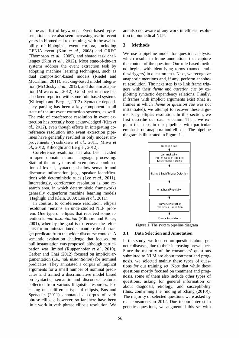
frame as a list of keywords. Event-based repre-sentations have also seen increasing use in recent years in biomedical text mining, with the availa-bility of biological event corpora, including GENIA event (Kim et al., 2008) and GREC (Thompson et al., 2009), and shared task chal-lenges (Kim et al., 2012). Most state-of-the-art systems address the event extraction task by adopting machine learning techniques, such as dual composition-based models (Riedel and McCallum, 2011), stacking-based model integra-tion (McClosky et al., 2012), and domain adapta-tion (Miwa et al., 2012). Good performance has also been reported with some rule-based systems (Kilicoglu and Bergler, 2012). Syntactic depend-ency parsing has been a key component in all state-of-the-art event extraction systems, as well. The role of coreference resolution in event ex-traction has recently been acknowledged (Kim et al., 2012), even though efforts in integrating co-reference resolution into event extraction pipe-lines have generally resulted in only modest im-provements (Yoshikawa et al., 2011; Miwa et al., 2012; Kilicoglu and Bergler, 2012).
Coreference resolution has also been tackled in open domain natural language processing. State-of-the-art systems often employ a combina-tion of lexical, syntactic, shallow semantic and discourse information (e.g., speaker identifica-tion) with deterministic rules (Lee et al., 2011). Interestingly, coreference resolution is one re-search area, in which deterministic frameworks generally outperform machine learning models (Haghighi and Klein, 2009; Lee et al., 2011).
In contrast to coreference resolution, ellipsis resolution remains an understudied NLP prob-lem. One type of ellipsis that received some at-tention is null instantiation (Fillmore and Baker, 2001), whereby the goal is to recover the refer-ents for an uninstantiated semantic role of a tar-get predicate from the wider discourse context. A semantic evaluation challenge that focused on null instantiation was proposed, although partici-pation was limited (Ruppenhofer et al., 2010). Gerber and Chai (2012) focused on implicit ar-gumentation (i.e., null instantiation) for nominal predicates. They annotated a corpus of implicit arguments for a small number of nominal predi-cates and trained a discriminative model based on syntactic, semantic and discourse features collected from various linguistic resources. Fo-cusing on a different type of ellipsis, Bos and Spenader (2011) annotated a corpus of verb phrase ellipsis; however, so far there have been little work in verb phrase ellipsis resolution. We
are also not aware of any work in ellipsis resolu-tion in biomedical NLP.
3 Methods
We use a pipeline model for question analysis, which results in frame annotations that capture the content of the question. Our rule-based meth-od begins with identifying terms (named enti-ties/triggers) in question text. Next, we recognize anaphoric mentions and, if any, perform anapho-ra resolution. The next step is to link frame trig-gers with their theme and question cue by ex-ploiting syntactic dependency relations. Finally, if frames with implicit arguments exist (that is, frames in which theme or question cue was not instantiated), we attempt to recover these argu-ments by ellipsis resolution. In this section, we first describe our data selection. Then, we ex-plain the steps in our pipeline, with particular emphasis on anaphora and ellipsis. The pipeline diagram is illustrated in Figure 1.
Figure 1. The system pipeline diagram
3.1 Data Selection and Annotation
In this study, we focused on questions about ge-netic diseases, due to their increasing prevalence. Since the majority of the consumers’ questions submitted to NLM are about treatment and prog-nosis, we selected mainly these types of ques-tions for our training set. Note that while these questions mostly focused on treatment and prog-nosis, some of them also include other types of questions, asking for general information or about diagnosis, etiology, and susceptibility (thus, confirming the finding of Zhang (2010)). The majority of selected questions were asked by real consumers in 2012. Due to our interest in genetics questions, we augmented this set with
56
some frequently asked questions from the Genet-ic and Rare Disease Information Center (GARD) 1 . Our selection yielded 32 treatment and 22 prognosis questions. An example treat-ment question was provided earlier (1). The fol-lowing is a training question on prognosis:
(2) They have diagnosed my niece with Salla disease. I understand that this is a very rare disease and that its main origin is Finland. Can you please let me know what to expect? My niece is 7 years old. It has taken them 6 years to finally come up with this diagnosis.
We used training questions to gain linguistic insights into the problem, to develop and refine our methodology, and as the basis of a trig-ger/question cue dictionary.
After the system was developed, we selected 29 previously unseen treatment-focused ques-tions posed to GARD for testing. We annotated them with target frames (41 instances) using brat annotation tool (Stenetorp et al., 2012) and eval-uated our system results against these frames. 29 of the target frames were treatment frames. Addi-tionally, there were 1 etiology, 6 general infor-mation, 2 diagnosis, and 3 prognosis frames.
3.2 Syntactic Dependency Parsing
Our question analysis module uses typed de-pendency relations as the basis of syntactic in-formation. We extract syntactic dependencies using Stanford Parser (de Marneffe et al., 2006) and use its collapsed dependency format. We rely on Stanford Parser for tokenization, lemma-tization, and part-of-speech tagging, as well.
3.3 Named Entity/Trigger Detection
We use simple dictionary lookup to map entity mentions in text to UMLS Metathesaurus con-cepts (Lindberg, 1993). So far, we have focused on recognizing three mention categories: prob-lems, interventions, and patients. Based on UMLS 2007AC release, we constructed a dic-tionary of string/concept pairs. We limited the dictionary to concepts with predefined semantic types. For example, all problems in the diction-ary have a semantic type that belongs to the Dis-orders semantic group (McCray et al., 2001), such as Neoplastic Process and Congenital Ab-normality. Currently our dictionary contains ap-proximately 260K string/concept pairs.
Dictionary lookup is also used to detect trig-gers and question cues. We constructed a trigger 1 https://rarediseases.info.nih.gov/GARD/
and question cue dictionary based on training data and limited expansion. The dictionary cur-rently contains 117 triggers and 14 question cues.
3.4 Recognizing Anaphoric Mentions
We focus on identifying two types of anaphoric phenomena: pronominal anaphora (including anaphora of personal and demonstrative pro-nouns) and sortal anaphora. The following ex-amples from the training questions illustrate these types. Anaphoric mentions are underlined and their antecedents are in bold. • Personal pronominal anaphora: My daughter
has just been diagnosed with Meier-Gorlin syndrome. I would like to learn more about it …
• Demonstrative pronominal anaphora: We just found out that our grandson has 48,XXYY syndrome. … I was wondering if you could give us some information on what to expect and the prognosis for this and ..
• Sortal anaphora: I have a 24-month-old niece who has the following symptoms of Cohen syndrome: … I would like seek your help in learning more about this condition.
To recognize mentions of personal pronominal and sortal anaphora, we mainly adapted the rule-based techniques outlined in Kilicoglu and Ber-gler (2012), itself based on the deterministic co-reference resolution approach described in Haghighi and Klein (2009). While Kilicoglu and Bergler (2012) focused on anaphora involving gene/protein terms, our adaptation focuses on those involving problems and patients. In addi-tion, we expanded their work by developing rules to recognize demonstrative pronominal anapho-ra.
3.4.1 Personal Pronouns
Kilicoglu and Bergler (2012) focused on only resolving it and they, since, in scientific article genre, resolving other third person pronouns (he, she) was less relevant. We currently recognize these two pronouns, as well. For personal pro-nouns, we merely tag the word as a pronominal anaphor if it is tagged as a pronoun and is in third person (i.e., she, he, it, they).
3.4.2 Demonstrative Pronouns
We rely on typed syntactic dependencies as well as part-of-speech tags to recognize demonstrative pronominal anaphora. A word is tagged as demonstrative pronominal anaphor if it is one of this, that, those, or these and if it is not the de-
57
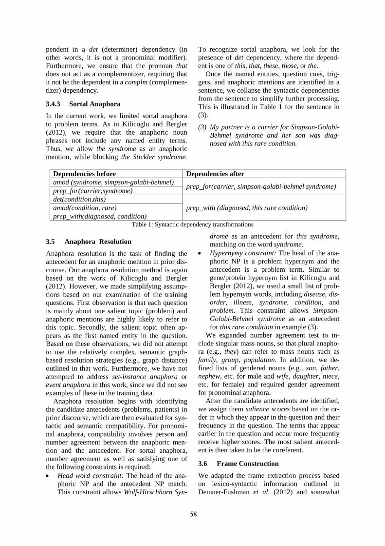
pendent in a det (determiner) dependency (in other words, it is not a pronominal modifier). Furthermore, we ensure that the pronoun that does not act as a complementizer, requiring that it not be the dependent in a complm (complemen-tizer) dependency.
3.4.3 Sortal Anaphora
In the current work, we limited sortal anaphora to problem terms. As in Kilicoglu and Bergler (2012), we require that the anaphoric noun phrases not include any named entity terms. Thus, we allow the syndrome as an anaphoric mention, while blocking the Stickler syndrome.
To recognize sortal anaphora, we look for the presence of det dependency, where the depend-ent is one of this, that, these, those, or the.
Once the named entities, question cues, trig-gers, and anaphoric mentions are identified in a sentence, we collapse the syntactic dependencies from the sentence to simplify further processing. This is illustrated in Table 1 for the sentence in (3).
(3) My partner is a carrier for Simpson-Golabi-Behmel syndrome and her son was diag-nosed with this rare condition.
Dependencies before Dependencies after amod (syndrome, simpson-golabi-behmel) prep_for(carrier, simpson-golabi-behmel syndrome) prep_for(carrier,syndrome) det(condition,this)
prep_with (diagnosed, this rare condition) amod(condition, rare) prep_with(diagnosed, condition)
Table 1: Syntactic dependency transformations
3.5 Anaphora Resolution
Anaphora resolution is the task of finding the antecedent for an anaphoric mention in prior dis-course. Our anaphora resolution method is again based on the work of Kilicoglu and Bergler (2012). However, we made simplifying assump-tions based on our examination of the training questions. First observation is that each question is mainly about one salient topic (problem) and anaphoric mentions are highly likely to refer to this topic. Secondly, the salient topic often ap-pears as the first named entity in the question. Based on these observations, we did not attempt to use the relatively complex, semantic graph-based resolution strategies (e.g., graph distance) outlined in that work. Furthermore, we have not attempted to address set-instance anaphora or event anaphora in this work, since we did not see examples of these in the training data.
Anaphora resolution begins with identifying the candidate antecedents (problems, patients) in prior discourse, which are then evaluated for syn-tactic and semantic compatibility. For pronomi-nal anaphora, compatibility involves person and number agreement between the anaphoric men-tion and the antecedent. For sortal anaphora, number agreement as well as satisfying one of the following constraints is required: • Head word constraint: The head of the ana-
phoric NP and the antecedent NP match. This constraint allows Wolf-Hirschhorn Syn-
drome as an antecedent for this syndrome, matching on the word syndrome.
• Hypernymy constraint: The head of the ana-phoric NP is a problem hypernym and the antecedent is a problem term. Similar to gene/protein hypernym list in Kilicoglu and Bergler (2012), we used a small list of prob-lem hypernym words, including disease, dis-order, illness, syndrome, condition, and problem. This constraint allows Simpson-Golabi-Behmel syndrome as an antecedent for this rare condition in example (3).
We expanded number agreement test to in-clude singular mass nouns, so that plural anapho-ra (e.g., they) can refer to mass nouns such as family, group, population. In addition, we de-fined lists of gendered nouns (e.g., son, father, nephew, etc. for male and wife, daughter, niece, etc. for female) and required gender agreement for pronominal anaphora.
After the candidate antecedents are identified, we assign them salience scores based on the or-der in which they appear in the question and their frequency in the question. The terms that appear earlier in the question and occur more frequently receive higher scores. The most salient anteced-ent is then taken to be the coreferent.
3.6 Frame Construction
We adapted the frame extraction process based on lexico-syntactic information outlined in Demner-Fushman et al. (2012) and somewhat
58
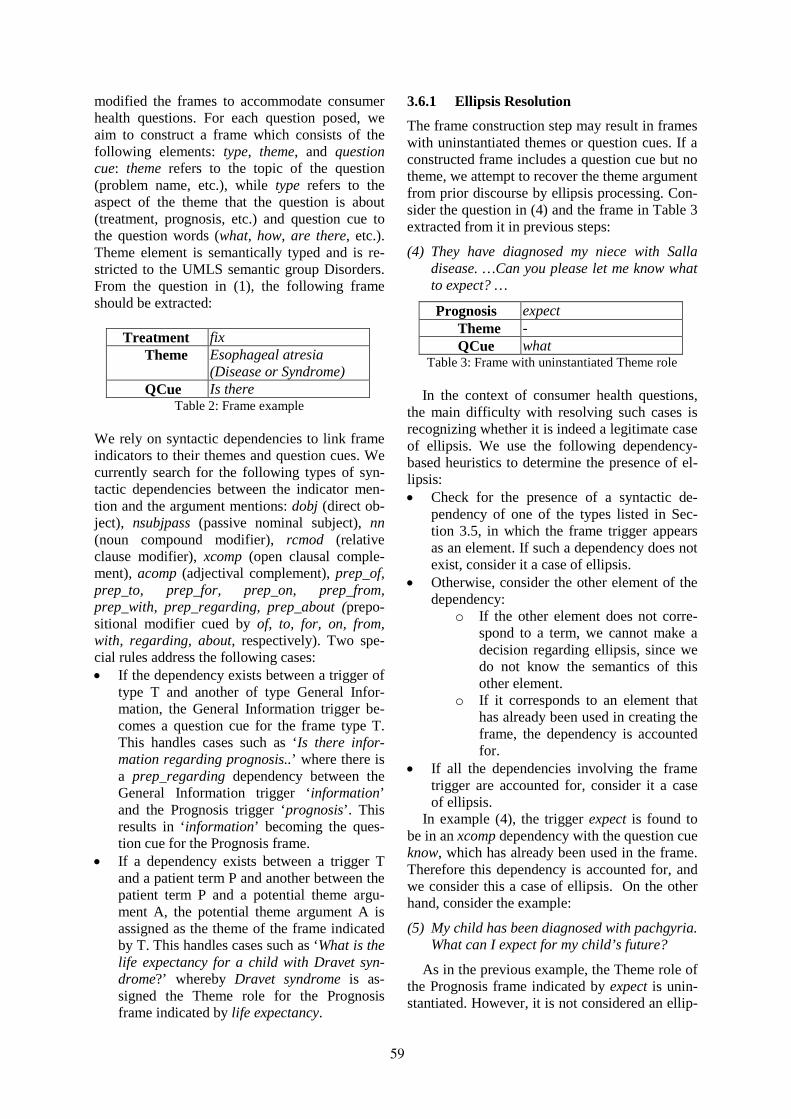
modified the frames to accommodate consumer health questions. For each question posed, we aim to construct a frame which consists of the following elements: type, theme, and question cue: theme refers to the topic of the question (problem name, etc.), while type refers to the aspect of the theme that the question is about (treatment, prognosis, etc.) and question cue to the question words (what, how, are there, etc.). Theme element is semantically typed and is re-stricted to the UMLS semantic group Disorders. From the question in (1), the following frame should be extracted:
Treatment fix Theme Esophageal atresia
(Disease or Syndrome) QCue Is there
Table 2: Frame example We rely on syntactic dependencies to link frame indicators to their themes and question cues. We currently search for the following types of syn-tactic dependencies between the indicator men-tion and the argument mentions: dobj (direct ob-ject), nsubjpass (passive nominal subject), nn (noun compound modifier), rcmod (relative clause modifier), xcomp (open clausal comple-ment), acomp (adjectival complement), prep_of, prep_to, prep_for, prep_on, prep_from, prep_with, prep_regarding, prep_about (prepo-sitional modifier cued by of, to, for, on, from, with, regarding, about, respectively). Two spe-cial rules address the following cases: • If the dependency exists between a trigger of
type T and another of type General Infor-mation, the General Information trigger be-comes a question cue for the frame type T. This handles cases such as ‘Is there infor-mation regarding prognosis..’ where there is a prep_regarding dependency between the General Information trigger ‘information’ and the Prognosis trigger ‘prognosis’. This results in ‘information’ becoming the ques-tion cue for the Prognosis frame.
• If a dependency exists between a trigger T and a patient term P and another between the patient term P and a potential theme argu-ment A, the potential theme argument A is assigned as the theme of the frame indicated by T. This handles cases such as ‘What is the life expectancy for a child with Dravet syn-drome?’ whereby Dravet syndrome is as-signed the Theme role for the Prognosis frame indicated by life expectancy.
3.6.1 Ellipsis Resolution
The frame construction step may result in frames with uninstantiated themes or question cues. If a constructed frame includes a question cue but no theme, we attempt to recover the theme argument from prior discourse by ellipsis processing. Con-sider the question in (4) and the frame in Table 3 extracted from it in previous steps:
(4) They have diagnosed my niece with Salla disease. …Can you please let me know what to expect? …
Prognosis expect Theme - QCue what
Table 3: Frame with uninstantiated Theme role
In the context of consumer health questions, the main difficulty with resolving such cases is recognizing whether it is indeed a legitimate case of ellipsis. We use the following dependency-based heuristics to determine the presence of el-lipsis: • Check for the presence of a syntactic de-
pendency of one of the types listed in Sec-tion 3.5, in which the frame trigger appears as an element. If such a dependency does not exist, consider it a case of ellipsis.
• Otherwise, consider the other element of the dependency:
o If the other element does not corre-spond to a term, we cannot make a decision regarding ellipsis, since we do not know the semantics of this other element.
o If it corresponds to an element that has already been used in creating the frame, the dependency is accounted for.
• If all the dependencies involving the frame trigger are accounted for, consider it a case of ellipsis.
In example (4), the trigger expect is found to be in an xcomp dependency with the question cue know, which has already been used in the frame. Therefore this dependency is accounted for, and we consider this a case of ellipsis. On the other hand, consider the example:
(5) My child has been diagnosed with pachgyria. What can I expect for my child’s future?
As in the previous example, the Theme role of the Prognosis frame indicated by expect is unin-stantiated. However, it is not considered an ellip-
59
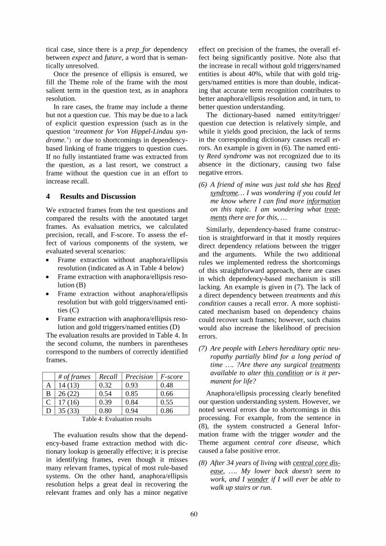
tical case, since there is a prep_for dependency between expect and future, a word that is seman-tically unresolved.
Once the presence of ellipsis is ensured, we fill the Theme role of the frame with the most salient term in the question text, as in anaphora resolution.
In rare cases, the frame may include a theme but not a question cue. This may be due to a lack of explicit question expression (such as in the question ‘treatment for Von Hippel-Lindau syn-drome.’) or due to shortcomings in dependency-based linking of frame triggers to question cues. If no fully instantiated frame was extracted from the question, as a last resort, we construct a frame without the question cue in an effort to increase recall.
4 Results and Discussion
We extracted frames from the test questions and compared the results with the annotated target frames. As evaluation metrics, we calculated precision, recall, and F-score. To assess the ef-fect of various components of the system, we evaluated several scenarios: • Frame extraction without anaphora/ellipsis
resolution (indicated as A in Table 4 below) • Frame extraction with anaphora/ellipsis reso-
lution (B) • Frame extraction without anaphora/ellipsis
resolution but with gold triggers/named enti-ties (C)
• Frame extraction with anaphora/ellipsis reso-lution and gold triggers/named entities (D)
The evaluation results are provided in Table 4. In the second column, the numbers in parentheses correspond to the numbers of correctly identified frames. # of frames Recall Precision F-score A 14 (13) 0.32 0.93 0.48 B 26 (22) 0.54 0.85 0.66 C 17 (16) 0.39 0.84 0.55 D 35 (33) 0.80 0.94 0.86
Table 4: Evaluation results
The evaluation results show that the depend-ency-based frame extraction method with dic-tionary lookup is generally effective; it is precise in identifying frames, even though it misses many relevant frames, typical of most rule-based systems. On the other hand, anaphora/ellipsis resolution helps a great deal in recovering the relevant frames and only has a minor negative
effect on precision of the frames, the overall ef-fect being significantly positive. Note also that the increase in recall without gold triggers/named entities is about 40%, while that with gold trig-gers/named entities is more than double, indicat-ing that accurate term recognition contributes to better anaphora/ellipsis resolution and, in turn, to better question understanding.
The dictionary-based named entity/trigger/ question cue detection is relatively simple, and while it yields good precision, the lack of terms in the corresponding dictionary causes recall er-rors. An example is given in (6). The named enti-ty Reed syndrome was not recognized due to its absence in the dictionary, causing two false negative errors.
(6) A friend of mine was just told she has Reed syndrome… I was wondering if you could let me know where I can find more information on this topic. I am wondering what treat-ments there are for this, …
Similarly, dependency-based frame construc-tion is straightforward in that it mostly requires direct dependency relations between the trigger and the arguments. While the two additional rules we implemented redress the shortcomings of this straightforward approach, there are cases in which dependency-based mechanism is still lacking. An example is given in (7). The lack of a direct dependency between treatments and this condition causes a recall error. A more sophisti-cated mechanism based on dependency chains could recover such frames; however, such chains would also increase the likelihood of precision errors.
(7) Are people with Lebers hereditary optic neu-ropathy partially blind for a long period of time …. ?Are there any surgical treatments available to alter this condition or is it per-manent for life?
Anaphora/ellipsis processing clearly benefited our question understanding system. However, we noted several errors due to shortcomings in this processing. For example, from the sentence in (8), the system constructed a General Infor-mation frame with the trigger wonder and the Theme argument central core disease, which caused a false positive error.
(8) After 34 years of living with central core dis-ease, …. My lower back doesn't seem to work, and I wonder if I will ever be able to walk up stairs or run.
60
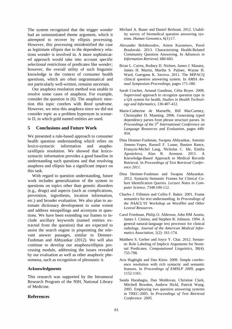
The system recognized that the trigger wonder had an uninstantiated theme argument, which it attempted to recover by ellipsis processing. However, this processing misidentified the case as legitimate ellipsis due to the dependency rela-tions wonder is involved in. A more sophisticat-ed approach would take into account specific selectional restrictions of predicates like wonder; however, the overall utility of such linguistic knowledge in the context of consumer health questions, which are often ungrammatical and not particularly well-written, remains uncertain.
Our anaphora resolution method was unable to resolve some cases of anaphora. For example, consider the question in (6). The anaphoric men-tion this topic corefers with Reed syndrome. However, we miss this anaphora since we did not consider topic as a problem hypernym in scenar-io D, in which gold named entities are used.
5 Conclusions and Future Work
We presented a rule-based approach to consumer health question understanding which relies on lexico-syntactic information and anapho-ra/ellipsis resolution. We showed that lexico-syntactic information provides a good baseline in understanding such questions and that resolving anaphora and ellipsis has a significant impact on this task.
With regard to question understanding, future work includes generalization of the system to questions on topics other than genetic disorders (e.g., drugs) and aspects (such as complications, prevention, ingredients, location information, etc.) and broader evaluation. We also plan to au-tomate dictionary development to some extent and address misspellings and acronyms in ques-tions. We have been extending our frames to in-clude ancillary keywords (named entities ex-tracted from the question) that are expected to assist the search engine in pinpointing the rele-vant answer passages, similar to Demner-Fushman and Abhyankar (2012). We will also continue to develop our anaphora/ellipsis pro-cessing module, addressing the issues revealed by our evaluation as well as other anaphoric phe-nomena, such as recognition of pleonastic it.
Acknowledgments
This research was supported by the Intramural Research Program of the NIH, National Library of Medicine.
References
Michael A. Bauer and Daniel Berleant. 2012. Usabil-ity survey of biomedical question answering sys-tems. Human Genomics, 6(1):17.
Alexander Beloborodov, Artem Kuznetsov, Pavel Braslavski. 2013. Characterizing Health-Related Community Question Answering. In Advances in Information Retrieval, 680-683.
Brian L. Cairns, Rodney D. Nielsen, James J. Masanz, James H. Martin, Martha S. Palmer, Wayne H. Ward, Guergana K. Savova. 2011. The MiPACQ clinical question answering system. In AMIA An-nual Symposium Proceedings, pages 171-180.
Sarah Cruchet, Arnaud Gaudinat, Célia Boyer. 2008. Supervised approach to recognize question type in a QA system for health. Studies in Health Technol-ogy and Informatics, 136:407-412.
Marie-Catherine de Marneffe, Bill MacCartney, Christopher D. Manning. 2006. Generating typed dependency parses from phrase structure parses. In Proceedings of the 5th International Conference on Language Resources and Evaluation, pages 449-454.
Dina Demner-Fushman, Swapna Abhyankar, Antonio Jimeno-Yepes, Russell F. Loane, Bastien Rance, François-Michel Lang, Nicholas C. Ide, Emilia Apostolova, Alan R. Aronson. 2011. A Knowledge-Based Approach to Medical Records Retrieval. In Proceedings of Text Retrieval Confer-ence 2011.
Dina Demner-Fushman and Swapna Abhyankar. 2012. Syntactic-Semantic Frames for Clinical Co-hort Identification Queries. Lecture Notes in Com-puter Science, 7348:100-112.
Charles J. Fillmore and Collin F. Baker. 2001. Frame semantics for text understanding. In Proceedings of the NAACL’01 Workshop on WordNet and Other Lexical Resources.
Carol Friedman, Philip O. Alderson, John HM Austin, James J. Cimino, and Stephen B. Johnson. 1994. A general natural-language text processor for clinical radiology. Journal of the American Medical Infor-matics Association, 1(2): 161-174.
Matthew S. Gerber and Joyce Y. Chai. 2012. Seman-tic Role Labeling of Implicit Arguments for Nomi-nal Predicates. Computational Linguistics, 38(4): 755-798.
Aria Haghighi and Dan Klein. 2009. Simple corefer-ence resolution with rich syntactic and semantic features. In Proceedings of EMNLP 2009, pages 1152-1161.
Sanda Harabagiu, Dan Moldovan, Christine Clark, Mitchell Bowden, Andrew Hickl, Patrick Wang. 2005. Employing two question answering systems in TREC-2005. In Proceedings of Text Retrieval Conference 2005.
61
Andrew Hickl, John Williams, Jeremy Bensley, Kirk Roberts, Ying Shi, Bryan Rink. 2006. Question Answering with LCC’s CHAUCER at TREC 2006. In Proceedings of Text Retrieval Conference 2006.
Lawrence Hunter and Kevin B. Cohen. 2006. Bio-medical language processing: what's beyond Pub-Med? Molecular Cell. 21(5):589-94.
Halil Kilicoglu and Sabine Bergler 2012. Biological Event Composition. BMC Bioinformatics, 13 (Supplement 11):S7.
Jin-Dong Kim, Tomoko Ohta, and Jun’ichi Tsujii. 2008. Corpus annotation for mining biomedical events from literature. BMC Bioinformatics, 9:10.
Jin-Dong Kim, Ngan Nguyen, Yue Wang, Jun’ichi Tsujii, Toshihisa Takagi, Akinori Yonezawa. 2012. The Genia Event and Protein Coreference tasks of the BioNLP Shared Task 2011. BMC Bioinformat-ics, 13(Supplement 11):S1.
Adam Lally, John M. Prager, Michael C. McCord, Branimir Boguraev, Siddharth Patwardhan, James Fan, Paul Fodor, Jennifer Chu-Carroll. 2012. Ques-tion analysis: How Watson reads a clue. IBM Jour-nal of Research and Development, 56(3):2.
Heeyoung Lee, Yves Peirsman, Angel Chang, Na-thanael Chambers, Mihai Surdeanu, Dan Jurafsky. 2011. Stanford's Multi-Pass Sieve Coreference Resolution System at the CoNLL-2011 Shared Task. In Proceedings of the CoNLL-2011 Shared Task, pages 28-34.
Donald A.B. Lindberg, Betsy L. Humphreys, Alexa T. McCray. 1993. The Unified Medical Language System. Methods of information in medicine, 32(4): 281-291.
Feifan Liu, Lamont D. Antieau, Hong Yu. 2011. To-ward automated consumer question answering: au-tomatically separating consumer questions from professional questions in the healthcare domain. Journal of Biomedical Informatics, 44(6): 1032-1038.
David McClosky, Sebastian Riedel, Mihai Surdeanu, Andrew McCallum, Christopher Manning. 2012. Combining joint models for biomedical event ex-traction. BMC Bioinformatics, 13 (Supplement 11): S9.
Alexa McCray, Russell Loane, Allen Browne, Anan-tha Bangalore. 1999. Terminology issues in user access to Web-based medical information. In AMIA Annual Symposium Proceedings, pages 107–111.
Alexa McCray, Anita Burgun, Olivier Bodenreider. 2001. Aggregating UMLS semantic types for re-ducing conceptual complexity. In Proceedings of Medinfo, 10(Pt1): 216-220.
Makoto Miwa, Paul Thompson, Sophia Ananiadou. 2012. Boosting automatic event extraction from the literature using domain adaptation and coreference resolution. Bioinformatics, 28(13):1759-1765.
Yuan Ni, Huijia Zhu, Peng Cai, Lei Zhang, Zhaoming Qui, Feng Cao. 2012. CliniQA: highly reliable clinical question answering system. Studies in Health Technology and Information, 180:215-219.
John M. Prager. 2006. Open-domain question answer-ing. Foundations and Trends in Information Re-trieval, 1(2):91-231.
Sebastian Riedel and Andrew McCallum. 2011. Fast and robust joint models for biomedical event ex-traction. In Proceedings of EMNLP 2011, pages 1-12.
Josef Ruppenhofer, Caroline Sporleder, Roser Mo-rante, Collin Baker, Martha Palmer. 2010. SemEval-2010 Task 10: Linking Events and Their Participants in Discourse. In Proceedings of the 5th International Workshop on Semantic Evaluation, pages 45-50.
Matthew S. Simpson and Dina Demner-Fushman. 2012. Biomedical Text Mining: a Survey of Recent Progress. Mining Text Data 2012:465-517.
Amanda Spink, Yin Yang, Jim Jansen, Pirrko Nykanen, Daniel P. Lorence, Seda Ozmutlu, H. Cenk Ozmutlu. 2004. A study of medical and health queries to web search engines. Health In-formation & Libraries Journal. 21(1):44-51.
Pontus Stenetorp, Sampo Pyysalo, Goran Topić, Tomoko Ohta, Sophia Ananiadou, Jun’ichi Tsujii. 2012. Brat: a Web-based Tool for NLP-Assisted Text Annotation. In Proceedings of the Demon-strations Sessions at EACL 2012, pages 102-107.
Paul Thompson, Syed A. Iqbal, John McNaught, So-phia Ananiadou. 2009. Construction of an annotat-ed corpus to support biomedical information ex-traction. BMC Bioinformatics, 10:349.
José L. Vicedo and Antonio Ferrández. 2000. Im-portance of pronominal anaphora resolution in question answering systems. In Proceedings of the 38th Annual Meeting on Association for Computa-tional Linguistics, pages 555-562.
Katsumasa Yoshikawa, Sebastian Riedel, Tsutomu Hirao, Masayuki Asahara, Yuji Matsumoto. 2011. Coreference Based Event-Argument Relation Ex-traction on Biomedical Text. Journal of Biomedi-cal Semantics, 2 (Supplement 5):S6.
Yan Zhang. 2010. Contextualizing Consumer Health Information Searching: an Analysis of Questions in a Social Q&A Community. In Proceedings of the 1st ACM International Health Informatics Sympo-sium (IHI’10), pages 210-219.
62
Proceedings of the 2013 Workshop on Biomedical Natural Language Processing (BioNLP 2013), pages 63–71,Sofia, Bulgaria, August 4-9 2013. c©2013 Association for Computational Linguistics
Evaluating large-scale text mining applicationsbeyond the traditional numeric performance measures
Sofie Van Landeghem1,2, Suwisa Kaewphan3,4, Filip Ginter3, Yves Van de Peer1,2
1. Dept. of Plant Systems Biology, VIB, Belgium2. Dept. of Plant Biotechnology and Bioinformatics, Ghent University, Belgium
3. Dept. of Information Technology, University of Turku, Finland4. Turku Centre for Computer Science (TUCS), Turku, Finland
[email protected], [email protected]@cs.utu.fi, [email protected]
Abstract
Text mining methods for the biomedicaldomain have matured substantially andare currently being applied on a largescale to support a variety of applica-tions in systems biology, pathway cura-tion, data integration and gene summa-rization. Community-wide challenges inthe BioNLP research field provide gold-standard datasets and rigorous evaluationcriteria, allowing for a meaningful com-parison between techniques as well asmeasuring progress within the field. How-ever, such evaluations are typically con-ducted on relatively small training andtest datasets. On a larger scale, sys-tematic erratic behaviour may occur thatseverely influences hundreds of thousandsof predictions. In this work, we per-form a critical assessment of a large-scaletext mining resource, identifying system-atic errors and determining their underly-ing causes through semi-automated analy-ses and manual evaluations1.
1 Introduction
The development and adaptation of natural lan-guage processing (NLP) techniques for thebiomedical domain are of crucial importance tomanage the abundance of available literature. Theinherent ambiguity of gene names and complex-ity of biomolecular interactions present an intrigu-ing challenge both for BioNLP researchers as wellas their targeted audience of biologists, geneticistsand bioinformaticians. Stimulating such research,various community-wide challenges have been or-ganised and received international participation.
1The supplementary data of this study is freely avail-able from http://bioinformatics.psb.ugent.be/supplementary_data/solan/bionlp13/
The BioCreative (BC) challenge (Hirschman etal., 2005; Krallinger et al., 2008; Leitner et al.,2010; Arighi et al., 2011) touches upon a variety ofextraction targets. The identification of gene andprotein mentions (‘named entity recognition’) is acentral task and a prerequisite for any follow-upwork in BioNLP. Linking these mentions to theirrespective gene database identifiers, ‘gene normal-ization’, is a crucial step to allow for integrationof textual information with authoritative databasesand experimental results. Other BC tasks are en-gaged in finding functional and physical relationsbetween gene products, including Gene Ontologyannotations and protein-protein interactions.
Focusing more specifically on the molecu-lar interactions between genes and proteins, theBioNLP Shared Task on Event Extraction (Kim etal., 2009; Kim et al., 2011b; Nedellec and others,2013) covers a number of detailed molecular eventtypes, including binding and transcription, regula-tory control and post-translational modifications.Additionally, separate tracks involve specific ap-plications of event extraction, including infectiousdiseases, bacterial biotopes and cancer genetics.
Performance of the participants in each of thesechallenges is measured using numeric metricssuch as precision, recall, F-measure, slot errorrate, MAP and TAP scores. While such rig-urous evaluations allow for a meaningful compar-ison between different systems, it is often difficultto translate these numeric values into a measure-ment of practical utility when applied on a largescale. Additionally, infrequent but consistent er-rors are often not identified through small-scaleevaluations, though they may result in hundreds ofthousands of wrongly predicted interactions on alarger scale. In this work, we perform an in-depthstudy of an open-source state-of-the-art event ex-traction system which was previously applied tothe whole of PubMed. Moving beyond the tra-ditional numeric evaluations, we identify a num-
63
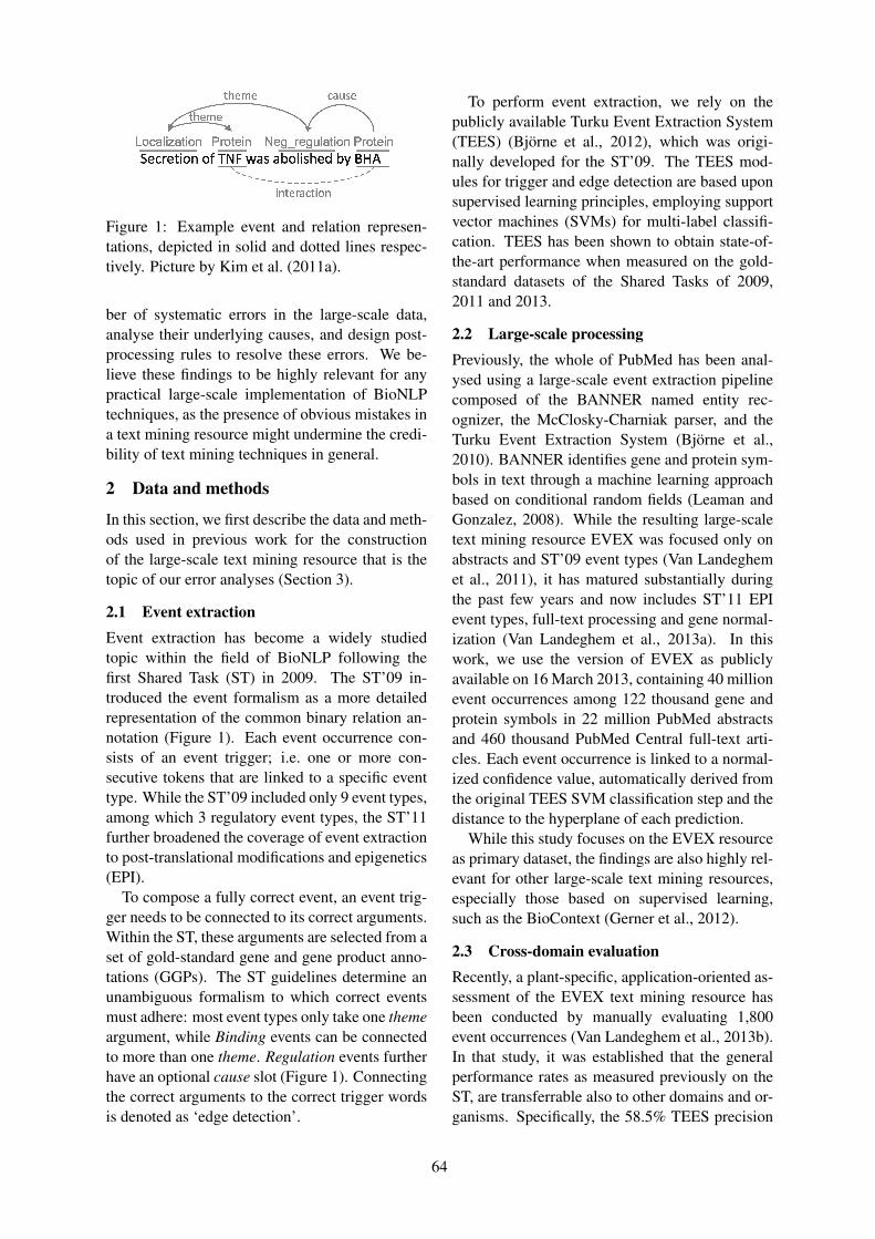
Figure 1: Example event and relation represen-tations, depicted in solid and dotted lines respec-tively. Picture by Kim et al. (2011a).
ber of systematic errors in the large-scale data,analyse their underlying causes, and design post-processing rules to resolve these errors. We be-lieve these findings to be highly relevant for anypractical large-scale implementation of BioNLPtechniques, as the presence of obvious mistakes ina text mining resource might undermine the credi-bility of text mining techniques in general.
2 Data and methods
In this section, we first describe the data and meth-ods used in previous work for the constructionof the large-scale text mining resource that is thetopic of our error analyses (Section 3).
2.1 Event extractionEvent extraction has become a widely studiedtopic within the field of BioNLP following thefirst Shared Task (ST) in 2009. The ST’09 in-troduced the event formalism as a more detailedrepresentation of the common binary relation an-notation (Figure 1). Each event occurrence con-sists of an event trigger; i.e. one or more con-secutive tokens that are linked to a specific eventtype. While the ST’09 included only 9 event types,among which 3 regulatory event types, the ST’11further broadened the coverage of event extractionto post-translational modifications and epigenetics(EPI).
To compose a fully correct event, an event trig-ger needs to be connected to its correct arguments.Within the ST, these arguments are selected from aset of gold-standard gene and gene product anno-tations (GGPs). The ST guidelines determine anunambiguous formalism to which correct eventsmust adhere: most event types only take one themeargument, while Binding events can be connectedto more than one theme. Regulation events furtherhave an optional cause slot (Figure 1). Connectingthe correct arguments to the correct trigger wordsis denoted as ‘edge detection’.
To perform event extraction, we rely on thepublicly available Turku Event Extraction System(TEES) (Bjorne et al., 2012), which was origi-nally developed for the ST’09. The TEES mod-ules for trigger and edge detection are based uponsupervised learning principles, employing supportvector machines (SVMs) for multi-label classifi-cation. TEES has been shown to obtain state-of-the-art performance when measured on the gold-standard datasets of the Shared Tasks of 2009,2011 and 2013.
2.2 Large-scale processingPreviously, the whole of PubMed has been anal-ysed using a large-scale event extraction pipelinecomposed of the BANNER named entity rec-ognizer, the McClosky-Charniak parser, and theTurku Event Extraction System (Bjorne et al.,2010). BANNER identifies gene and protein sym-bols in text through a machine learning approachbased on conditional random fields (Leaman andGonzalez, 2008). While the resulting large-scaletext mining resource EVEX was focused only onabstracts and ST’09 event types (Van Landeghemet al., 2011), it has matured substantially duringthe past few years and now includes ST’11 EPIevent types, full-text processing and gene normal-ization (Van Landeghem et al., 2013a). In thiswork, we use the version of EVEX as publiclyavailable on 16 March 2013, containing 40 millionevent occurrences among 122 thousand gene andprotein symbols in 22 million PubMed abstractsand 460 thousand PubMed Central full-text arti-cles. Each event occurrence is linked to a normal-ized confidence value, automatically derived fromthe original TEES SVM classification step and thedistance to the hyperplane of each prediction.
While this study focuses on the EVEX resourceas primary dataset, the findings are also highly rel-evant for other large-scale text mining resources,especially those based on supervised learning,such as the BioContext (Gerner et al., 2012).
2.3 Cross-domain evaluationRecently, a plant-specific, application-oriented as-sessment of the EVEX text mining resource hasbeen conducted by manually evaluating 1,800event occurrences (Van Landeghem et al., 2013b).In that study, it was established that the generalperformance rates as measured previously on theST, are transferrable also to other domains and or-ganisms. Specifically, the 58.5% TEES precision
64
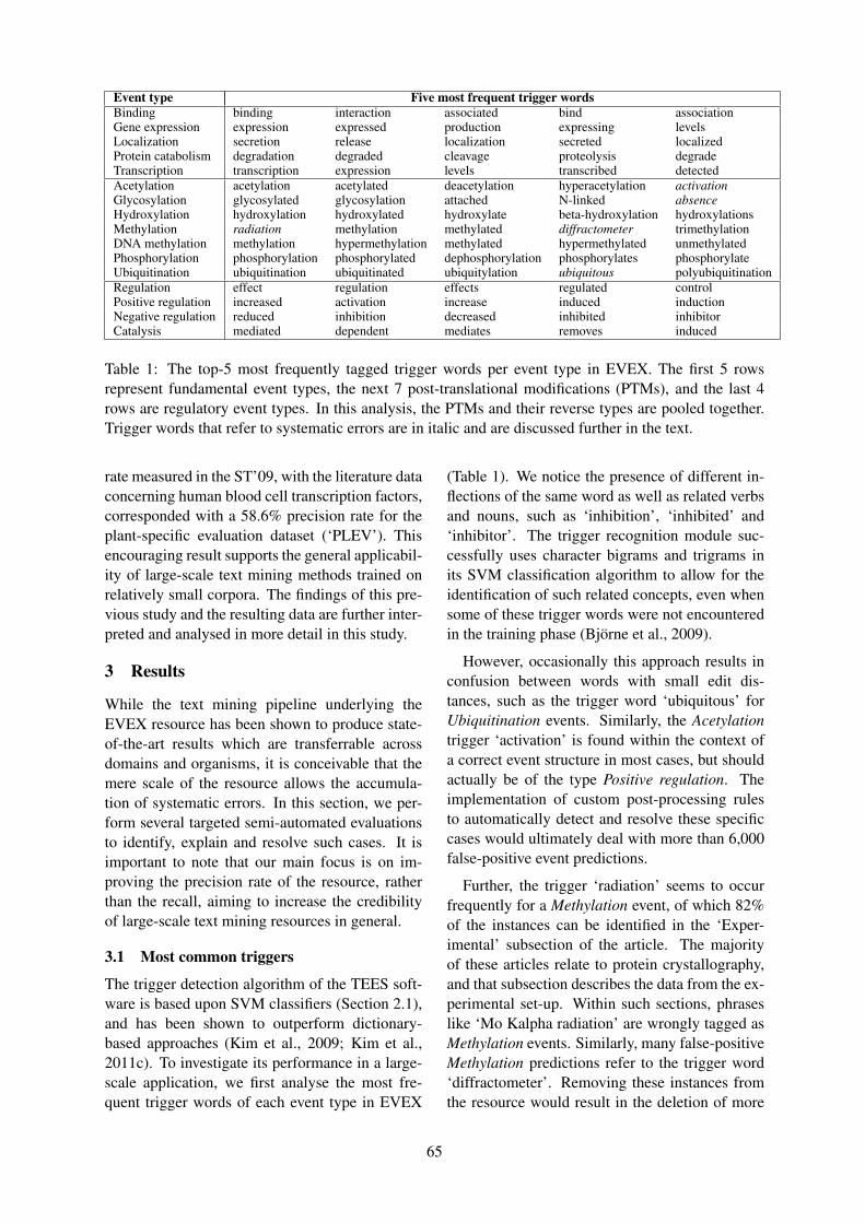
Event type Five most frequent trigger wordsBinding binding interaction associated bind associationGene expression expression expressed production expressing levelsLocalization secretion release localization secreted localizedProtein catabolism degradation degraded cleavage proteolysis degradeTranscription transcription expression levels transcribed detectedAcetylation acetylation acetylated deacetylation hyperacetylation activationGlycosylation glycosylated glycosylation attached N-linked absenceHydroxylation hydroxylation hydroxylated hydroxylate beta-hydroxylation hydroxylationsMethylation radiation methylation methylated diffractometer trimethylationDNA methylation methylation hypermethylation methylated hypermethylated unmethylatedPhosphorylation phosphorylation phosphorylated dephosphorylation phosphorylates phosphorylateUbiquitination ubiquitination ubiquitinated ubiquitylation ubiquitous polyubiquitinationRegulation effect regulation effects regulated controlPositive regulation increased activation increase induced inductionNegative regulation reduced inhibition decreased inhibited inhibitorCatalysis mediated dependent mediates removes induced
Table 1: The top-5 most frequently tagged trigger words per event type in EVEX. The first 5 rowsrepresent fundamental event types, the next 7 post-translational modifications (PTMs), and the last 4rows are regulatory event types. In this analysis, the PTMs and their reverse types are pooled together.Trigger words that refer to systematic errors are in italic and are discussed further in the text.
rate measured in the ST’09, with the literature dataconcerning human blood cell transcription factors,corresponded with a 58.6% precision rate for theplant-specific evaluation dataset (‘PLEV’). Thisencouraging result supports the general applicabil-ity of large-scale text mining methods trained onrelatively small corpora. The findings of this pre-vious study and the resulting data are further inter-preted and analysed in more detail in this study.
3 Results
While the text mining pipeline underlying theEVEX resource has been shown to produce state-of-the-art results which are transferrable acrossdomains and organisms, it is conceivable that themere scale of the resource allows the accumula-tion of systematic errors. In this section, we per-form several targeted semi-automated evaluationsto identify, explain and resolve such cases. It isimportant to note that our main focus is on im-proving the precision rate of the resource, ratherthan the recall, aiming to increase the credibilityof large-scale text mining resources in general.
3.1 Most common triggers
The trigger detection algorithm of the TEES soft-ware is based upon SVM classifiers (Section 2.1),and has been shown to outperform dictionary-based approaches (Kim et al., 2009; Kim et al.,2011c). To investigate its performance in a large-scale application, we first analyse the most fre-quent trigger words of each event type in EVEX
(Table 1). We notice the presence of different in-flections of the same word as well as related verbsand nouns, such as ‘inhibition’, ‘inhibited’ and‘inhibitor’. The trigger recognition module suc-cessfully uses character bigrams and trigrams inits SVM classification algorithm to allow for theidentification of such related concepts, even whensome of these trigger words were not encounteredin the training phase (Bjorne et al., 2009).
However, occasionally this approach results inconfusion between words with small edit dis-tances, such as the trigger word ‘ubiquitous’ forUbiquitination events. Similarly, the Acetylationtrigger ‘activation’ is found within the context ofa correct event structure in most cases, but shouldactually be of the type Positive regulation. Theimplementation of custom post-processing rulesto automatically detect and resolve these specificcases would ultimately deal with more than 6,000false-positive event predictions.
Further, the trigger ‘radiation’ seems to occurfrequently for a Methylation event, of which 82%of the instances can be identified in the ‘Exper-imental’ subsection of the article. The majorityof these articles relate to protein crystallography,and that subsection describes the data from the ex-perimental set-up. Within such sections, phraseslike ‘Mo Kalpha radiation’ are wrongly tagged asMethylation events. Similarly, many false-positiveMethylation predictions refer to the trigger word‘diffractometer’. Removing these instances fromthe resource would result in the deletion of more
65
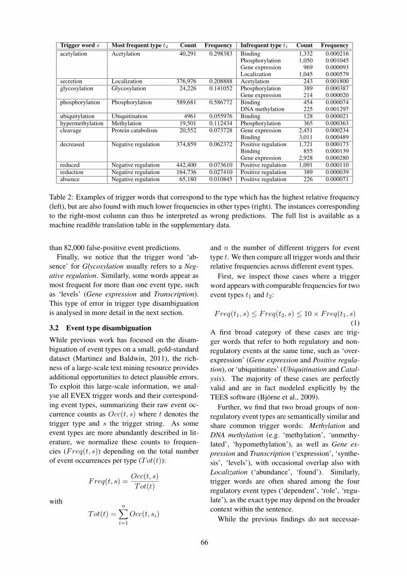
Trigger word s Most frequent type t2 Count Frequency Infrequent type t1 Count Frequencyacetylation Acetylation 40,291 0.298383 Binding 1,332 0.000216
Phosphorylation 1,050 0.001045Gene expression 969 0.000093Localization 1,045 0.000579
secretion Localization 376,976 0.208888 Acetylation 243 0.001800glycosylation Glycosylation 24,226 0.141052 Phosphorylation 389 0.000387
Gene expression 214 0.000020phosphorylation Phosphorylation 589,681 0.586772 Binding 454 0.000074
DNA methylation 225 0.001297ubiquitylation Ubiquitination 4961 0.055976 Binding 128 0.000021hypermethylation Methylation 19,501 0.112434 Phosphorylation 365 0.000363cleavage Protein catabolism 20,552 0.073728 Gene expression 2,451 0.000234
Binding 3,011 0.000489decreased Negative regulation 374,859 0.062372 Positive regulation 1,721 0.000173
Binding 855 0.000139Gene expression 2,928 0.000280
reduced Negative regulation 442,400 0.073610 Positive regulation 1,091 0.000110reduction Negative regulation 164,736 0.027410 Positive regulation 389 0.000039absence Negative regulation 65,180 0.010845 Positive regulation 226 0.000071
Table 2: Examples of trigger words that correspond to the type which has the highest relative frequency(left), but are also found with much lower frequencies in other types (right). The instances correspondingto the right-most column can thus be interpreted as wrong predictions. The full list is available as amachine readible translation table in the supplementary data.
than 82,000 false-positive event predictions.Finally, we notice that the trigger word ‘ab-
sence’ for Glycosylation usually refers to a Neg-ative regulation. Similarly, some words appear asmost frequent for more than one event type, suchas ‘levels’ (Gene expression and Transcription).This type of error in trigger type disambiguationis analysed in more detail in the next section.
3.2 Event type disambiguationWhile previous work has focused on the disam-biguation of event types on a small, gold-standarddataset (Martinez and Baldwin, 2011), the rich-ness of a large-scale text mining resource providesadditional opportunities to detect plausible errors.To exploit this large-scale information, we anal-yse all EVEX trigger words and their correspond-ing event types, summarizing their raw event oc-currence counts as Occ(t, s) where t denotes thetrigger type and s the trigger string. As someevent types are more abundantly described in lit-erature, we normalize these counts to frequen-cies (Freq(t, s)) depending on the total numberof event occurrences per type (Tot(t)):
Freq(t, s) =Occ(t, s)
Tot(t)
with
Tot(t) =n∑
i=1
Occ(t, si)
and n the number of different triggers for eventtype t. We then compare all trigger words and theirrelative frequencies across different event types.
First, we inspect those cases where a triggerword appears with comparable frequencies for twoevent types t1 and t2:
Freq(t1, s) ≤ Freq(t2, s) ≤ 10× Freq(t1, s)(1)
A first broad category of these cases are trig-ger words that refer to both regulatory and non-regulatory events at the same time, such as ‘over-expression’ (Gene expression and Positive regula-tion), or ‘ubiquitinates’ (Ubiquitination and Catal-ysis). The majority of these cases are perfectlyvalid and are in fact modeled explicitly by theTEES software (Bjorne et al., 2009).
Further, we find that two broad groups of non-regulatory event types are semantically similar andshare common trigger words: Methylation andDNA methylation (e.g. ‘methylation’, ‘unmethy-lated’, ‘hypomethylation’), as well as Gene ex-pression and Transcription (‘expression’, ‘synthe-sis’, ‘levels’), with occasional overlap also withLocalization (‘abundance’, ‘found’). Similarly,trigger words are often shared among the fourregulatory event types (‘dependent’, ‘role’, ‘regu-late’), as the exact type may depend on the broadercontext within the sentence.
While the previous findings do not necessar-
66
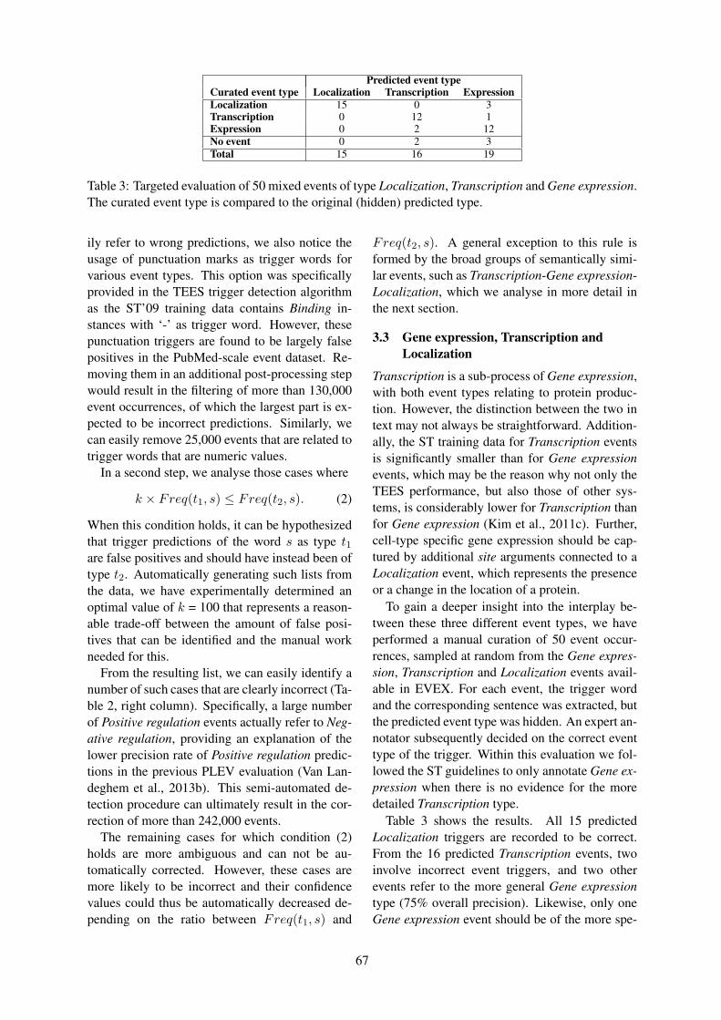
Predicted event typeCurated event type Localization Transcription ExpressionLocalization 15 0 3Transcription 0 12 1Expression 0 2 12No event 0 2 3Total 15 16 19
Table 3: Targeted evaluation of 50 mixed events of type Localization, Transcription and Gene expression.The curated event type is compared to the original (hidden) predicted type.
ily refer to wrong predictions, we also notice theusage of punctuation marks as trigger words forvarious event types. This option was specificallyprovided in the TEES trigger detection algorithmas the ST’09 training data contains Binding in-stances with ‘-’ as trigger word. However, thesepunctuation triggers are found to be largely falsepositives in the PubMed-scale event dataset. Re-moving them in an additional post-processing stepwould result in the filtering of more than 130,000event occurrences, of which the largest part is ex-pected to be incorrect predictions. Similarly, wecan easily remove 25,000 events that are related totrigger words that are numeric values.
In a second step, we analyse those cases where
k × Freq(t1, s) ≤ Freq(t2, s). (2)
When this condition holds, it can be hypothesizedthat trigger predictions of the word s as type t1are false positives and should have instead been oftype t2. Automatically generating such lists fromthe data, we have experimentally determined anoptimal value of k = 100 that represents a reason-able trade-off between the amount of false posi-tives that can be identified and the manual workneeded for this.
From the resulting list, we can easily identify anumber of such cases that are clearly incorrect (Ta-ble 2, right column). Specifically, a large numberof Positive regulation events actually refer to Neg-ative regulation, providing an explanation of thelower precision rate of Positive regulation predic-tions in the previous PLEV evaluation (Van Lan-deghem et al., 2013b). This semi-automated de-tection procedure can ultimately result in the cor-rection of more than 242,000 events.
The remaining cases for which condition (2)holds are more ambiguous and can not be au-tomatically corrected. However, these cases aremore likely to be incorrect and their confidencevalues could thus be automatically decreased de-pending on the ratio between Freq(t1, s) and
Freq(t2, s). A general exception to this rule isformed by the broad groups of semantically simi-lar events, such as Transcription-Gene expression-Localization, which we analyse in more detail inthe next section.
3.3 Gene expression, Transcription andLocalization
Transcription is a sub-process of Gene expression,with both event types relating to protein produc-tion. However, the distinction between the two intext may not always be straightforward. Addition-ally, the ST training data for Transcription eventsis significantly smaller than for Gene expressionevents, which may be the reason why not only theTEES performance, but also those of other sys-tems, is considerably lower for Transcription thanfor Gene expression (Kim et al., 2011c). Further,cell-type specific gene expression should be cap-tured by additional site arguments connected to aLocalization event, which represents the presenceor a change in the location of a protein.
To gain a deeper insight into the interplay be-tween these three different event types, we haveperformed a manual curation of 50 event occur-rences, sampled at random from the Gene expres-sion, Transcription and Localization events avail-able in EVEX. For each event, the trigger wordand the corresponding sentence was extracted, butthe predicted event type was hidden. An expert an-notator subsequently decided on the correct eventtype of the trigger. Within this evaluation we fol-lowed the ST guidelines to only annotate Gene ex-pression when there is no evidence for the moredetailed Transcription type.
Table 3 shows the results. All 15 predictedLocalization triggers are recorded to be correct.From the 16 predicted Transcription events, twoinvolve incorrect event triggers, and two otherevents refer to the more general Gene expressiontype (75% overall precision). Likewise, only oneGene expression event should be of the more spe-
67
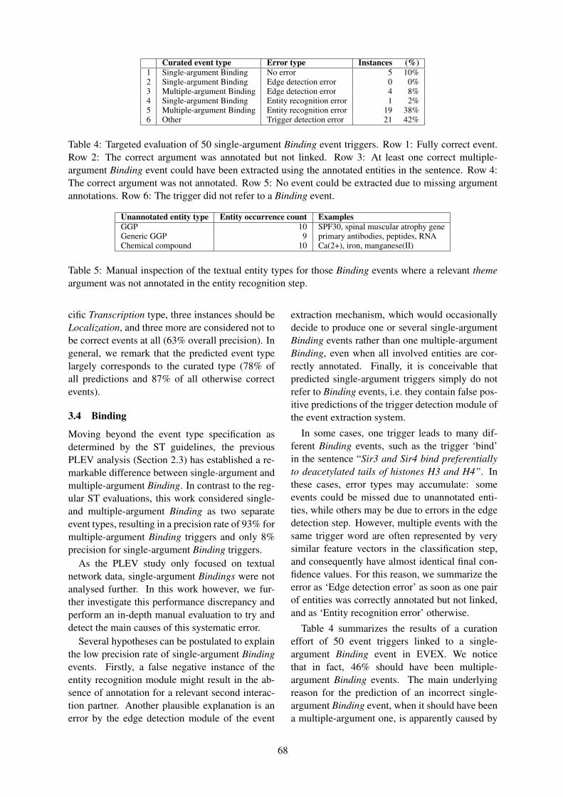
Curated event type Error type Instances (%)1 Single-argument Binding No error 5 10%2 Single-argument Binding Edge detection error 0 0%3 Multiple-argument Binding Edge detection error 4 8%4 Single-argument Binding Entity recognition error 1 2%5 Multiple-argument Binding Entity recognition error 19 38%6 Other Trigger detection error 21 42%
Table 4: Targeted evaluation of 50 single-argument Binding event triggers. Row 1: Fully correct event.Row 2: The correct argument was annotated but not linked. Row 3: At least one correct multiple-argument Binding event could have been extracted using the annotated entities in the sentence. Row 4:The correct argument was not annotated. Row 5: No event could be extracted due to missing argumentannotations. Row 6: The trigger did not refer to a Binding event.
Unannotated entity type Entity occurrence count ExamplesGGP 10 SPF30, spinal muscular atrophy geneGeneric GGP 9 primary antibodies, peptides, RNAChemical compound 10 Ca(2+), iron, manganese(II)
Table 5: Manual inspection of the textual entity types for those Binding events where a relevant themeargument was not annotated in the entity recognition step.
cific Transcription type, three instances should beLocalization, and three more are considered not tobe correct events at all (63% overall precision). Ingeneral, we remark that the predicted event typelargely corresponds to the curated type (78% ofall predictions and 87% of all otherwise correctevents).
3.4 Binding
Moving beyond the event type specification asdetermined by the ST guidelines, the previousPLEV analysis (Section 2.3) has established a re-markable difference between single-argument andmultiple-argument Binding. In contrast to the reg-ular ST evaluations, this work considered single-and multiple-argument Binding as two separateevent types, resulting in a precision rate of 93% formultiple-argument Binding triggers and only 8%precision for single-argument Binding triggers.
As the PLEV study only focused on textualnetwork data, single-argument Bindings were notanalysed further. In this work however, we fur-ther investigate this performance discrepancy andperform an in-depth manual evaluation to try anddetect the main causes of this systematic error.
Several hypotheses can be postulated to explainthe low precision rate of single-argument Bindingevents. Firstly, a false negative instance of theentity recognition module might result in the ab-sence of annotation for a relevant second interac-tion partner. Another plausible explanation is anerror by the edge detection module of the event
extraction mechanism, which would occasionallydecide to produce one or several single-argumentBinding events rather than one multiple-argumentBinding, even when all involved entities are cor-rectly annotated. Finally, it is conceivable thatpredicted single-argument triggers simply do notrefer to Binding events, i.e. they contain false pos-itive predictions of the trigger detection module ofthe event extraction system.
In some cases, one trigger leads to many dif-ferent Binding events, such as the trigger ‘bind’in the sentence “Sir3 and Sir4 bind preferentiallyto deacetylated tails of histones H3 and H4”. Inthese cases, error types may accumulate: someevents could be missed due to unannotated enti-ties, while others may be due to errors in the edgedetection step. However, multiple events with thesame trigger word are often represented by verysimilar feature vectors in the classification step,and consequently have almost identical final con-fidence values. For this reason, we summarize theerror as ‘Edge detection error’ as soon as one pairof entities was correctly annotated but not linked,and as ‘Entity recognition error’ otherwise.
Table 4 summarizes the results of a curationeffort of 50 event triggers linked to a single-argument Binding event in EVEX. We noticethat in fact, 46% should have been multiple-argument Binding events. The main underlyingreason for the prediction of an incorrect single-argument Binding event, when it should have beena multiple-argument one, is apparently caused by
68
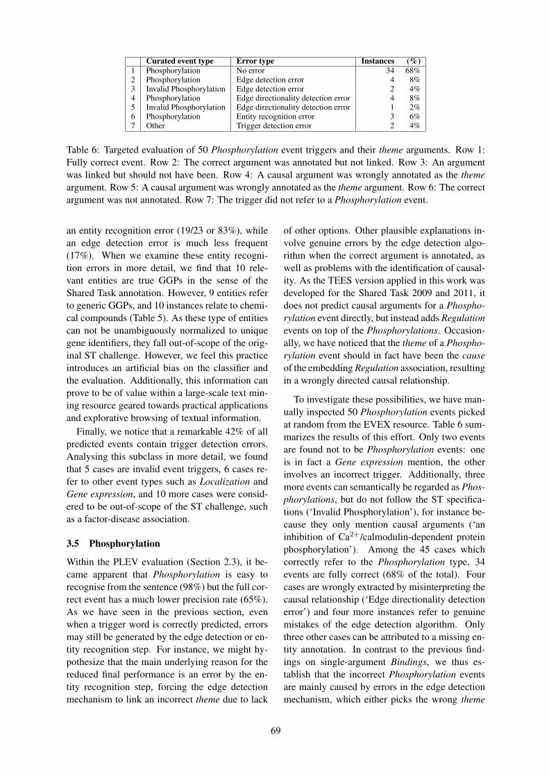
Curated event type Error type Instances (%)1 Phosphorylation No error 34 68%2 Phosphorylation Edge detection error 4 8%3 Invalid Phosphorylation Edge detection error 2 4%4 Phosphorylation Edge directionality detection error 4 8%5 Invalid Phosphorylation Edge directionality detection error 1 2%6 Phosphorylation Entity recognition error 3 6%7 Other Trigger detection error 2 4%
Table 6: Targeted evaluation of 50 Phosphorylation event triggers and their theme arguments. Row 1:Fully correct event. Row 2: The correct argument was annotated but not linked. Row 3: An argumentwas linked but should not have been. Row 4: A causal argument was wrongly annotated as the themeargument. Row 5: A causal argument was wrongly annotated as the theme argument. Row 6: The correctargument was not annotated. Row 7: The trigger did not refer to a Phosphorylation event.
an entity recognition error (19/23 or 83%), whilean edge detection error is much less frequent(17%). When we examine these entity recogni-tion errors in more detail, we find that 10 rele-vant entities are true GGPs in the sense of theShared Task annotation. However, 9 entities referto generic GGPs, and 10 instances relate to chemi-cal compounds (Table 5). As these type of entitiescan not be unambiguously normalized to uniquegene identifiers, they fall out-of-scope of the orig-inal ST challenge. However, we feel this practiceintroduces an artificial bias on the classifier andthe evaluation. Additionally, this information canprove to be of value within a large-scale text min-ing resource geared towards practical applicationsand explorative browsing of textual information.
Finally, we notice that a remarkable 42% of allpredicted events contain trigger detection errors.Analysing this subclass in more detail, we foundthat 5 cases are invalid event triggers, 6 cases re-fer to other event types such as Localization andGene expression, and 10 more cases were consid-ered to be out-of-scope of the ST challenge, suchas a factor-disease association.
3.5 Phosphorylation
Within the PLEV evaluation (Section 2.3), it be-came apparent that Phosphorylation is easy torecognise from the sentence (98%) but the full cor-rect event has a much lower precision rate (65%).As we have seen in the previous section, evenwhen a trigger word is correctly predicted, errorsmay still be generated by the edge detection or en-tity recognition step. For instance, we might hy-pothesize that the main underlying reason for thereduced final performance is an error by the en-tity recognition step, forcing the edge detectionmechanism to link an incorrect theme due to lack
of other options. Other plausible explanations in-volve genuine errors by the edge detection algo-rithm when the correct argument is annotated, aswell as problems with the identification of causal-ity. As the TEES version applied in this work wasdeveloped for the Shared Task 2009 and 2011, itdoes not predict causal arguments for a Phospho-rylation event directly, but instead adds Regulationevents on top of the Phosphorylations. Occasion-ally, we have noticed that the theme of a Phospho-rylation event should in fact have been the causeof the embedding Regulation association, resultingin a wrongly directed causal relationship.
To investigate these possibilities, we have man-ually inspected 50 Phosphorylation events pickedat random from the EVEX resource. Table 6 sum-marizes the results of this effort. Only two eventsare found not to be Phosphorylation events: oneis in fact a Gene expression mention, the otherinvolves an incorrect trigger. Additionally, threemore events can semantically be regarded as Phos-phorylations, but do not follow the ST specifica-tions (‘Invalid Phosphorylation’), for instance be-cause they only mention causal arguments (‘aninhibition of Ca2+/calmodulin-dependent proteinphosphorylation’). Among the 45 cases whichcorrectly refer to the Phosphorylation type, 34events are fully correct (68% of the total). Fourcases are wrongly extracted by misinterpreting thecausal relationship (‘Edge directionality detectionerror’) and four more instances refer to genuinemistakes of the edge detection algorithm. Onlythree other cases can be attributed to a missing en-tity annotation. In contrast to the previous find-ings on single-argument Bindings, we thus es-tablish that the incorrect Phosphorylation eventsare mainly caused by errors in the edge detectionmechanism, which either picks the wrong theme
69
from the set of annotated GGPs, or misinterpretsthe causality direction.
4 Discussion and conclusion
We have performed several semi-automated eval-uations and targeted manual curation experiments,identifying and explaining systematic errors in alarge-scale event dataset. As a first observation,we notice that a few frequent trigger words arealmost always associated to incorrect event pre-dictions, such as the trigger words ‘ubiquitous’and ‘radiation’, or a punctuation symbol. Thesecases were identified through a large-scale auto-matic analysis in combination with a limited man-ual evaluation effort. The results are distributed asa blacklist of event triggers for the implementationor filtering of future large-scale event predictionsefforts.
Further, a semi-automated procedure has iden-tified a list of likely incorrect predictions, bycomparing the type-specific frequencies of triggerwords across all event types. Manual inspection ofthe most frequent cases allowed us to determine anumber of trigger words for which the event typecan automatically be corrected. These results arealso made publicly available.
Additionally, after removal of the most obvi-ous and frequent errors, a fully automated scriptcan automatically reduce the confidence scores ofthose event occurrences where the trigger wordsare found to be much more frequent for anotherevent type. We have established that this proce-dure should disregard triggers identified within afew specific semantically similar clusters: DNAmethylation/Methylation, Regulation/Positive reg-ulation/Negative regulation/Catalysis and Geneexpression-Transcription/Localization. An addi-tional targeted evaluation of these last three typesrevealed that, despite their semantic overlap, thelargest fraction of these predictions refers to thecorrect event type (78± 11.5%).
Finally, we note that trigger detection (47 ±14.6%) and entity recognition errors (44±14.6%)are the main causes of wrongly predicted Bind-ing events. The latter causes the event extractionmechanism to artificially produce single-argumentBindings instead of multiple-argument Bindings.We believe this issue can be resolved by broaden-ing the scope of the entity recognition module togeneric GGPs and chemical compounds, and re-applying the TEES algorithm to these entities as
if they were normal GGPs as defined in the STformalism. In contrast, edge detection errors aremuch more frequently the cause of a wrongly pre-dicted Phosphorylation event (statistically signifi-cant difference with p < 0.05), caused by wronglyidentifying the thematic object or the causality ofthe event. To resolve this issue, we propose fu-ture annotation efforts to specifically annotate theprotein adding the phosphate group to the targetprotein as a separate class than the regulation ofsuch a phosphorylation process by other cellularmachineries and components (Kim et al., 2013).
In conclusion, we have performed severalstatistical analyses and targeted manual eval-uations on a large-scale event dataset. As aresult, we were able to identify a set of rulesto automatically delete or correct a numberof false positive predictions (supplementarymaterial at http://bioinformatics.psb.ugent.be/supplementary_data/solan/bionlp13/). When applying theserules to the winning submission of the recentST’13 (GE subchallenge), which was basedon the TEES classifier (Hakala et al., 2013),3 false positive predictions could be identifiedand removed. Even though this procedure onlymarginally improves the classification results(50.97% to 50.99% F-score), we believe thecleaning procedure to be crucial specifically forthe credibility of any large-scale text miningapplication. For example, applied on the EVEXresource, it would ultimately result in the removalof 242,000 instances and a corrected event type of230,000 more cases (1.2% of all EVEX events intotal). These corrections will be implemented aspart of the next big EVEX release. Additionally,the confidence score of more than 120,000 am-biguous cases could be automatically decreased.Alternatively, these cases could be the target ofa large-scale re-annotation, for instance usingthe brat annotation tool (Stenetorp et al., 2012).The resulting dataset could then serve as a newtraining set to enable active learning on top ofexisting event extraction approaches.
Acknowledgments
The authors thank Cindy Martens and the anony-mous reviewers for a critical reading of themanuscript and constructive feedback. SVLthanks the Research Foundation Flanders (FWO)for funding her research.
70
ReferencesCecilia Arighi, Zhiyong Lu, Martin Krallinger, Kevin
Cohen, J. Wilbur, Alfonso Valencia, LynetteHirschman, and Cathy Wu. 2011. Overview ofthe BioCreative III workshop. BMC Bioinformatics,12(Suppl 8):S1.
Jari Bjorne, Juho Heimonen, Filip Ginter, Antti Airola,Tapio Pahikkala, and Tapio Salakoski. 2009. Ex-tracting complex biological events with rich graph-based feature sets. In Proceedings of the BioNLP2009 Workshop, pages 10–18.
Jari Bjorne, Filip Ginter, Sampo Pyysalo, Jun’ichi Tsu-jii, and Tapio Salakoski. 2010. Scaling up biomed-ical event extraction to the entire PubMed. In Pro-ceedings of the BioNLP 2010 Workshop, pages 28–36.
Jari Bjorne, Filip Ginter, and Tapio Salakoski. 2012.Generalizing biomedical event extraction. BMCBioinformatics, 13(suppl. 8):S4.
Martin Gerner, Farzaneh Sarafraz, Casey M. Bergman,and Goran Nenadic. 2012. BioContext: an in-tegrated text mining system for large-scale extrac-tion and contextualization of biomolecular events.Bioinformatics, 28(16):2154–2161.
Kai Hakala, Sofie Van Landeghem, Tapio Salakoski,Yves Van de Peer, and Filip Ginter. 2013. EVEXin ST13: Application of a large-scale text miningresource to event extraction and network construc-tion. In Proceedings of the BioNLP Shared Task2013 Workshop (in press).
Lynette Hirschman, Alexander Yeh, ChristianBlaschke, and Alfonso Valencia. 2005. Overviewof BioCreAtIvE: critical assessment of informa-tion extraction for biology. BMC Bioinformatics,6(Suppl 1):S1.
Jin-Dong Kim, Tomoko Ohta, Sampo Pyysalo, Yoshi-nobu Kano, and Jun’ichi Tsujii. 2009. Overviewof BioNLP’09 Shared Task on event extraction. InProceedings of the BioNLP 2009 Workshop, pages1–9.
Jin-Dong Kim, Tomoko Ohta, Sampo Pyysalo, Yoshi-nobu Kano, and Junichi Tsujii. 2011a. Ex-tracting bio-molecular events from literature - theBioNLP’09 Shared Task. Computational Intelli-gence, 27(4):513–540.
Jin-Dong Kim, Sampo Pyysalo, Tomoko Ohta, RobertBossy, Ngan Nguyen, and Jun’ichi Tsujii. 2011b.Overview of BioNLP Shared Task 2011. In Pro-ceedings of the BioNLP Shared Task 2011 Work-shop, pages 1–6.
Jin-Dong Kim, Yue Wang, Toshihisa Takagi, and Aki-nori Yonezawa. 2011c. Overview of Genia eventtask in BioNLP Shared Task 2011. In Proceedingsof the BioNLP Shared Task 2011 Workshop, BioNLPShared Task ’11, pages 7–15.
Jin-Dong Kim, Yue Wang, Yamamoto Yasunori,Sabine Bergler, Roser Morante, and Kevin Cohen.2013. The Genia Event Extraction Shared Task,2013 edition - overview. In Proceedings of theBioNLP Shared Task 2013 Workshop (in press).
Martin Krallinger, Alexander Morgan, Larry Smith,Florian Leitner, Lorraine Tanabe, John Wilbur,Lynette Hirschman, and Alfonso Valencia. 2008.Evaluation of text-mining systems for biology:overview of the second BioCreative communitychallenge. Genome Biology, 9(Suppl 2):S1.
Robert Leaman and Graciela Gonzalez. 2008. BAN-NER: an executable survey of advances in biomedi-cal named entity recognition. Pacific Symposium onBiocomputing. Pacific Symposium on Biocomputing,pages 652–663.
F. Leitner, S.A. Mardis, M. Krallinger, G. Cesareni,L.A. Hirschman, and A. Valencia. 2010. Anoverview of BioCreative II.5. Computational Bi-ology and Bioinformatics, IEEE/ACM Transactionson, 7(3):385–399.
David Martinez and Timothy Baldwin. 2011. Wordsense disambiguation for event trigger word detec-tion in biomedicine. BMC Bioinformatics, 12(Suppl2):S4.
Claire Nedellec et al. 2013. Overview of BioNLPShared Task 2013. In Proceedings of the BioNLPShared Task 2013 Workshop (in press).
Pontus Stenetorp, Sampo Pyysalo, Goran Topic,Tomoko Ohta, Sophia Ananiadou, and Jun’ichi Tsu-jii. 2012. brat: a web-based tool for NLP-assistedtext annotation. In Proceedings of the Demonstra-tions at the 13th Conference of the European Chap-ter of the Association for Computational Linguistics,pages 102–107.
Sofie Van Landeghem, Filip Ginter, Yves Van de Peer,and Tapio Salakoski. 2011. EVEX: a PubMed-scaleresource for homology-based generalization of textmining predictions. In Proceedings of the BioNLP2011 Workshop, pages 28–37.
Sofie Van Landeghem, Jari Bjorne, Chih-Hsuan Wei,Kai Hakala, Sampo Pyysalo, Sophia Ananiadou,Hung-Yu Kao, Zhiyong Lu, Tapio Salakoski, YvesVan de Peer, and Filip Ginter. 2013a. Large-scale event extraction from literature with multi-level gene normalization. PLoS ONE, 8(4):e55814.
Sofie Van Landeghem, Stefanie De Bodt, Zuzanna J.Drebert, Dirk Inz, and Yves Van de Peer. 2013b.The potential of text mining in data integration andnetwork biology for plant research: A case study onarabidopsis. The Plant Cell, 25(3):794–807.
71
Proceedings of the 2013 Workshop on Biomedical Natural Language Processing (BioNLP 2013), pages 72–79,Sofia, Bulgaria, August 4-9 2013. c©2013 Association for Computational Linguistics
Recognizing sublanguages in scientific journal articlesthrough closure properties
Irina P. TemnikovaLinguistic Modelling LaboratoryBulgarian Academy of Sciences
K. Bretonnel CohenComputational Bioscience Program
University of Colorado School of MedicineDepartment of Linguistics
University of Colorado at [email protected]
Abstract
It has long been realized that sublanguagesare relevant to natural language process-ing and text mining. However, practicalmethods for recognizing or characterizingthem have been lacking. This paper de-scribes a publicly available set of tools forsublanguage recognition. Closure proper-ties are used to assess the goodness of fitof two biomedical corpora to the sublan-guage model. Scientific journal articlesare compared to general English text, andit is shown that the journal articles fit thesublanguage model, while the general En-glish text does not. A number of examplesof implications of the sublanguage char-acteristics for natural language processingare pointed out. The software is made pub-licly available at [edited for anonymiza-tion].
1 Introduction
1.1 Definitions of “sublanguage”
The notion of sublanguage has had varied defini-tions, depending on the aspects of sublanguageson which the authors focused. (Grishman and Kit-tredge, 1986) focus on syntactic aspects of sub-languages: “. . . the term suggests a subsystem oflanguage. . . limited in reference to a specific sub-ject domain. In particular, each sublanguage hasa distinctive grammar, which can profitably bedescribed and used to solve specific language-processing problems” (Grishman and Kittredge,1986).
(Kittredge, 2003) focuses on the spontaneousappearance of sublanguages in restricted domains,where the preconditions for a sublanguage to ap-pear are the sharing of specialized knowledgeabout a restricted semantic domain and recurrent
“situations” (e.g. scientific journal articles, or dis-charge summaries) in which domain experts com-municate. According to (Kittredge, 2003), charac-teristics of a sublanguage include a restricted lexi-con, relatively small number of lexical classes, re-stricted sentence syntax, deviant sentence syntax,restricted word co-occurrence patterns, and differ-ent frequencies of occurrence of words and syn-tactic patterns from the normal language.
(McDonald, 2000) focuses on the element of re-striction in sublanguages—the notion that they arerestricted to a specialized semantic domain, a very“focused” audience, and “stipulated content,” withthe effect that both word choice and syntactic stylehave reduced options as compared to the normallanguage.
The notions of restriction that recur in thesedefinitions of “sublanguage” lead directly to(McEnery and Wilson, 2001)’s notion of usingthe quantification of closure properties to assesswhether or not a given sample of a genre of lan-guage use fits the sublanguage model. Closurerefers to the tendency of a genre of language to-wards finiteness at one or more linguistic levels.For example, a genre of language might or mightnot use a finite set of lexical items, or have a fi-nite set of sentence structures. Notions of restric-tion suggest that a sublanguage should tend to-wards closure on at least some linguistic levels.To quantify closure, we can examine relationshipsbetween types and tokens in a corpus of the genre.In particular, we count the number of types thatare observed as an increasing number of tokensis examined. If a genre does not exhibit closure,then the number of types will continue to rise con-tinually as the number of tokens increases. Onthe other hand, closure is demonstrated when thenumber of types stops growing after some numberof tokens has been examined.
72
1.2 Relevance of sublanguages to naturallanguage processing
The relevance of sublanguages to natural languageprocessing has long been recognized in a vari-ety of fields. (Hirschman and Sager, 1982) and(Friedman, 1986) show how a sublanguage–basedapproach can be used for information extractionfrom clinical documents. (Finin, 1986) shows thatsublanguage characterization can be used for thenotoriously difficult problem of interpretation ofnominal compounds. (Sager, 1986) asserts a num-ber of uses for sublanguage–oriented natural lan-guage processing, including resolution of syntac-tic ambiguity, definition of frames for informa-tion extraction, and discourse analysis. (Sekine,1994) describes a prototype application of sublan-guages to speech recognition. (Friedman et al.,1994) uses a sublanguage grammar to extract a va-riety of types of structured data from clinical re-ports. (McDonald, 2000) points out that modernlanguage generation systems are made effective inlarge part due to the fact that they are applied tospecific sublanguages. (Somers, 2000) discussesthe relevance of sublanguages to machine trans-lation, pointing out that many sublanguages canmake machine translation easier and some of themcan make machine translation harder. (Friedmanet al., 2001) uses a sublanguage grammar to ex-tract structured data from scientific journal arti-cles.
1.3 Previous work on sublanguagerecognition
Various approaches have been taken to recog-nizing sublanguages. We posit here two sepa-rate tasks—recognizing a sublanguage when oneis present, and determining the characteristics ofa sublanguage. Information-theoretic approacheshave a long history. (Sekine, 1994) clustered docu-ments and then calculated the ratio of the perplex-ity of the clustered documents to the perplexityof a random collection of words. (Somers, 1998)showed that texts drawn from a sublanguage cor-pus have low weighted cumulative sums. (Stetsonet al., 2002) used relative entropy and squared chi-square distance to identify a sublanguage of cross-coverage notes. (Mihaila et al., 2012) looked atdistributions of named entities to identify and dif-ferentiate between a wide variety of scientific sub-languages.
Non-information-theoretic, more heuristic
methods have been used to identify sublanguages,as well. In addition to the information-theoreticmeasures described above, (Stetson et al., 2002)also looked at such measures as length, incidenceof abbreviations, and ambiguity of abbreviations.(Friedman et al., 2002) use manual analysis todetect and characterize two biomedical sublan-guages. (McEnery and Wilson, 2001) examineclosure properties; their approach is so central tothe topic of this paper that we will describe it insome length separately.
(McEnery and Wilson, 2001) examined the clo-sure properties of three linguistic aspects of theirmaterial under study. As materials they used twocorpora that were assumed not to meet the sub-language model—the Canadian Hansard corpus,containing proceedings from the Canadian Parlia-ment, and the American Printing House for theBlind corpus, made up of works of fiction. Asa corpus that was suspected to meet the sublan-guage model, they used a set of manuals fromIBM. All three corpora differed in size, so theywere sampled to match the size of the smallestcorpus, meaning that all experiments were doneon collections 200,000 words in size. The mate-rials under study were evaluated for their closureproperties at three linguistic levels. At the mostbasic level, they looked at lexical items—simpleword forms. The hypothesis here was that the non-sublanguage corpora would not tend toward finite-ness, i.e. would not reach closure. That is, if thenumber of word types found was graphed as anincreasing number of tokens was examined, theresulting line would grow continually and wouldshow no signs of asymptoting. In contrast, thesublanguage corpus would eventually reach clo-sure, i.e. would stop growing appreciably in sizeas more tokens were examined.
The next level that they examined was the mor-phosyntactic level. In particular, they looked atthe number of part-of-speech tags per lexical type.Here the intuition was that if the lexicon of thesublanguage is limited, then words might be co-erced into a greater number of parts of speech.This would be manifested by a smaller overallnumber of unique word/part-of-speech tag combi-nations. Again, we would expect to see that thesublanguage corpus would have a smaller numberof word/part-of-speech tag combinations, as com-pared to the non-sublanguage corpus. Graphingthe count of word type/POS tag sets on the y axis
73
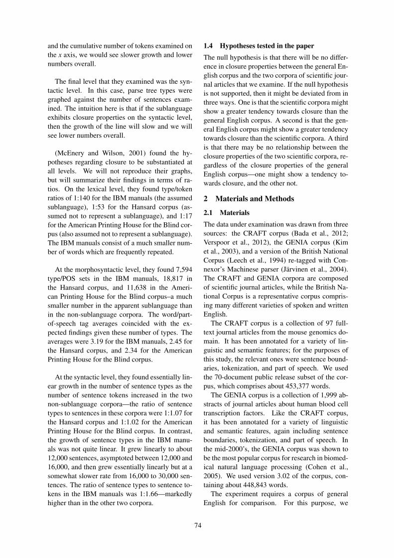
and the cumulative number of tokens examined onthe x axis, we would see slower growth and lowernumbers overall.
The final level that they examined was the syn-tactic level. In this case, parse tree types weregraphed against the number of sentences exam-ined. The intuition here is that if the sublanguageexhibits closure properties on the syntactic level,then the growth of the line will slow and we willsee lower numbers overall.
(McEnery and Wilson, 2001) found the hy-potheses regarding closure to be substantiated atall levels. We will not reproduce their graphs,but will summarize their findings in terms of ra-tios. On the lexical level, they found type/tokenratios of 1:140 for the IBM manuals (the assumedsublanguage), 1:53 for the Hansard corpus (as-sumed not to represent a sublanguage), and 1:17for the American Printing House for the Blind cor-pus (also assumed not to represent a sublanguage).The IBM manuals consist of a much smaller num-ber of words which are frequently repeated.
At the morphosyntactic level, they found 7,594type/POS sets in the IBM manuals, 18,817 inthe Hansard corpus, and 11,638 in the Ameri-can Printing House for the Blind corpus–a muchsmaller number in the apparent sublanguage thanin the non-sublanguage corpora. The word/part-of-speech tag averages coincided with the ex-pected findings given these number of types. Theaverages were 3.19 for the IBM manuals, 2.45 forthe Hansard corpus, and 2.34 for the AmericanPrinting House for the Blind corpus.
At the syntactic level, they found essentially lin-ear growth in the number of sentence types as thenumber of sentence tokens increased in the twonon-sublanguage corpora—the ratio of sentencetypes to sentences in these corpora were 1:1.07 forthe Hansard corpus and 1:1.02 for the AmericanPrinting House for the Blind corpus. In contrast,the growth of sentence types in the IBM manu-als was not quite linear. It grew linearly to about12,000 sentences, asymptoted between 12,000 and16,000, and then grew essentially linearly but at asomewhat slower rate from 16,000 to 30,000 sen-tences. The ratio of sentence types to sentence to-kens in the IBM manuals was 1:1.66—markedlyhigher than in the other two corpora.
1.4 Hypotheses tested in the paperThe null hypothesis is that there will be no differ-ence in closure properties between the general En-glish corpus and the two corpora of scientific jour-nal articles that we examine. If the null hypothesisis not supported, then it might be deviated from inthree ways. One is that the scientific corpora mightshow a greater tendency towards closure than thegeneral English corpus. A second is that the gen-eral English corpus might show a greater tendencytowards closure than the scientific corpora. A thirdis that there may be no relationship between theclosure properties of the two scientific corpora, re-gardless of the closure properties of the generalEnglish corpus—one might show a tendency to-wards closure, and the other not.
2 Materials and Methods
2.1 MaterialsThe data under examination was drawn from threesources: the CRAFT corpus (Bada et al., 2012;Verspoor et al., 2012), the GENIA corpus (Kimet al., 2003), and a version of the British NationalCorpus (Leech et al., 1994) re-tagged with Con-nexor’s Machinese parser (Jarvinen et al., 2004).The CRAFT and GENIA corpora are composedof scientific journal articles, while the British Na-tional Corpus is a representative corpus compris-ing many different varieties of spoken and writtenEnglish.
The CRAFT corpus is a collection of 97 full-text journal articles from the mouse genomics do-main. It has been annotated for a variety of lin-guistic and semantic features; for the purposes ofthis study, the relevant ones were sentence bound-aries, tokenization, and part of speech. We usedthe 70-document public release subset of the cor-pus, which comprises about 453,377 words.
The GENIA corpus is a collection of 1,999 ab-stracts of journal articles about human blood celltranscription factors. Like the CRAFT corpus,it has been annotated for a variety of linguisticand semantic features, again including sentenceboundaries, tokenization, and part of speech. Inthe mid-2000’s, the GENIA corpus was shown tobe the most popular corpus for research in biomed-ical natural language processing (Cohen et al.,2005). We used version 3.02 of the corpus, con-taining about 448,843 words.
The experiment requires a corpus of generalEnglish for comparison. For this purpose, we
74
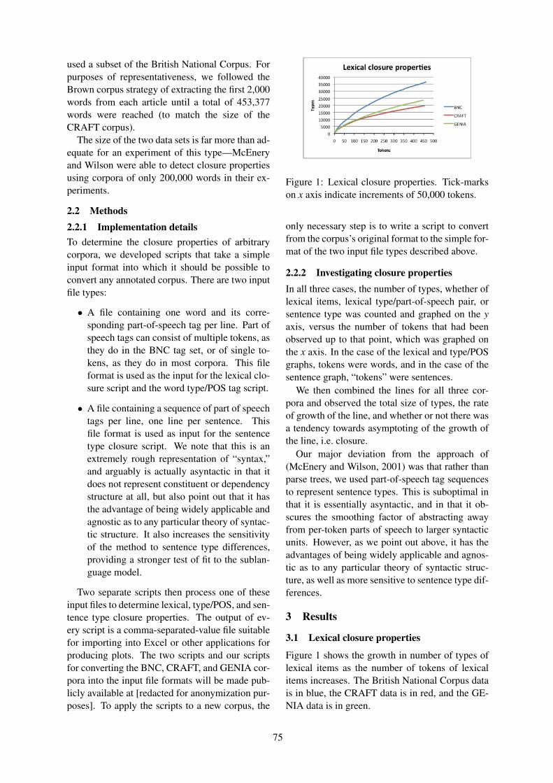
used a subset of the British National Corpus. Forpurposes of representativeness, we followed theBrown corpus strategy of extracting the first 2,000words from each article until a total of 453,377words were reached (to match the size of theCRAFT corpus).
The size of the two data sets is far more than ad-equate for an experiment of this type—McEneryand Wilson were able to detect closure propertiesusing corpora of only 200,000 words in their ex-periments.
2.2 Methods2.2.1 Implementation detailsTo determine the closure properties of arbitrarycorpora, we developed scripts that take a simpleinput format into which it should be possible toconvert any annotated corpus. There are two inputfile types:
• A file containing one word and its corre-sponding part-of-speech tag per line. Part ofspeech tags can consist of multiple tokens, asthey do in the BNC tag set, or of single to-kens, as they do in most corpora. This fileformat is used as the input for the lexical clo-sure script and the word type/POS tag script.
• A file containing a sequence of part of speechtags per line, one line per sentence. Thisfile format is used as input for the sentencetype closure script. We note that this is anextremely rough representation of “syntax,”and arguably is actually asyntactic in that itdoes not represent constituent or dependencystructure at all, but also point out that it hasthe advantage of being widely applicable andagnostic as to any particular theory of syntac-tic structure. It also increases the sensitivityof the method to sentence type differences,providing a stronger test of fit to the sublan-guage model.
Two separate scripts then process one of theseinput files to determine lexical, type/POS, and sen-tence type closure properties. The output of ev-ery script is a comma-separated-value file suitablefor importing into Excel or other applications forproducing plots. The two scripts and our scriptsfor converting the BNC, CRAFT, and GENIA cor-pora into the input file formats will be made pub-licly available at [redacted for anonymization pur-poses]. To apply the scripts to a new corpus, the
Figure 1: Lexical closure properties. Tick-markson x axis indicate increments of 50,000 tokens.
only necessary step is to write a script to convertfrom the corpus’s original format to the simple for-mat of the two input file types described above.
2.2.2 Investigating closure propertiesIn all three cases, the number of types, whether oflexical items, lexical type/part-of-speech pair, orsentence type was counted and graphed on the yaxis, versus the number of tokens that had beenobserved up to that point, which was graphed onthe x axis. In the case of the lexical and type/POSgraphs, tokens were words, and in the case of thesentence graph, “tokens” were sentences.
We then combined the lines for all three cor-pora and observed the total size of types, the rateof growth of the line, and whether or not there wasa tendency towards asymptoting of the growth ofthe line, i.e. closure.
Our major deviation from the approach of(McEnery and Wilson, 2001) was that rather thanparse trees, we used part-of-speech tag sequencesto represent sentence types. This is suboptimal inthat it is essentially asyntactic, and in that it ob-scures the smoothing factor of abstracting awayfrom per-token parts of speech to larger syntacticunits. However, as we point out above, it has theadvantages of being widely applicable and agnos-tic as to any particular theory of syntactic struc-ture, as well as more sensitive to sentence type dif-ferences.
3 Results
3.1 Lexical closure properties
Figure 1 shows the growth in number of types oflexical items as the number of tokens of lexicalitems increases. The British National Corpus datais in blue, the CRAFT data is in red, and the GE-NIA data is in green.
75
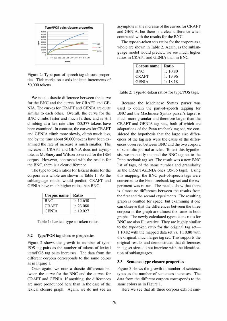
Figure 2: Type-part-of-speech tag closure proper-ties. Tick-marks on x axis indicate increments of50,000 tokens.
We note a drastic difference between the curvefor the BNC and the curves for CRAFT and GE-NIA. The curves for CRAFT and GENIA are quitesimilar to each other. Overall, the curve for theBNC climbs faster and much farther, and is stillclimbing at a fast rate after 453,377 tokens havebeen examined. In contrast, the curves for CRAFTand GENIA climb more slowly, climb much less,and by the time about 50,000 tokens have been ex-amined the rate of increase is much smaller. Theincrease in CRAFT and GENIA does not asymp-tote, as McEnery and Wilson observed for the IBMcorpus. However, contrasted with the results forthe BNC, there is a clear difference.
The type to token ratios for lexical items for thecorpora as a whole are shown in Table 1. As thesublanguage model would predict, CRAFT andGENIA have much higher ratios than BNC.
Corpus name RatioBNC 1: 12.650CRAFT 1: 23.080GENIA 1: 19.027
Table 1: Lexical type-to-token ratios.
3.2 Type/POS tag closure properties
Figure 2 shows the growth in number of type-POS tag pairs as the number of tokens of lexicalitem/POS tag pairs increases. The data from thedifferent corpora corresponds to the same colorsas in Figure 1.
Once again, we note a drastic difference be-tween the curve for the BNC and the curves forCRAFT and GENIA. If anything, the differencesare more pronounced here than in the case of thelexical closure graph. Again, we do not see an
asymptote in the increase of the curves for CRAFTand GENIA, but there is a clear difference whencontrasted with the results for the BNC.
The type-to-token sets ratios for the corpora as awhole are shown in Table 2. Again, as the sublan-guage model would predict, we see much higherratios in CRAFT and GENIA than in BNC.
Corpus name RatioBNC 1: 10.80CRAFT 1: 19.96GENIA 1: 18.18
Table 2: Type-to-token ratios for type/POS tags.
Because the Machinese Syntax parser wasused to obtain the part-of-speech tagging forBNC and the Machinese Syntax parser’s tagset ismuch more granular and therefore larger than theCRAFT and GENIA tag sets, both of which areadaptations of the Penn treebank tag set, we con-sidered the hypothesis that the large size differ-ences of the tag sets were the cause of the differ-ences observed between BNC and the two corporaof scientific journal articles. To test this hypothe-sis, we manually mapped the BNC tag set to thePenn treebank tag set. The result was a new BNClist of tags, of the same number and granularityas the CRAFT/GENIA ones (35-36 tags). Usingthis mapping, the BNC part-of-speech tags wereconverted to the Penn treebank tag set and the ex-periment was re-run. The results show that thereis almost no difference between the results fromthe first and the second experiments. The resultinggraph is omitted for space, but examining it onecan observe that the differences between the threecorpora in the graph are almost the same in bothgraphs. The newly calculated type:tokens ratio forBNC are also illustrative. They are highly similarto the type-token ratio for the original tag set—1:10.82 with the mapped data set vs. 1:10.80 withthe original, much larger tag set. This supports theoriginal results and demonstrates that differencesin tag set sizes do not interfere with the identifica-tion of sublanguages.
3.3 Sentence type closure properties
Figure 3 shows the growth in number of sentencetypes as the number of sentences increases. Thedata from the different corpora corresponds to thesame colors as in Figure 1.
Here we see that all three corpora exhibit sim-
76
Figure 3: Sentence type closure properties. Tick-marks on x axis indicate increments of 5,000 sen-tences.
ilar curves—essentially linear, with nearly identi-cal growth rates. This is a strong contrast with theresults seen in Figures 1 and 2. We suggest somereasons for this in the Discussion section.
The ratio of sentence types to sentence tokensfor the corpora as a whole are given in Table 3.As would be expected from the essentially lineargrowth observed with token growth for all threecorpora, all three ratios are nearly 1:1.
Corpus name RatioBNC 1: 1.03CRAFT 1: 1.14GENIA 1: 1.11
Table 3: Sentence type-to-token ratios.
4 Discussion and Conclusions
The most obvious conclusion of this study is thatthe null hypothesis can be rejected—the scien-tific corpora show a greater tendency towards clo-sure than the general English corpus. Further-more, we observe that the two scientific corporabehave quite similarly to each other at all threelevels. This second observation is not necessar-ily a given. If we can consider for a moment thenotion that there might be degrees of fit to the sub-language model, it is clear that from a content per-spective the BNC is unlimited; the CRAFT cor-pus is limited to mouse genomics, but not to anyparticular area of mouse genomics (indeed, it con-tains articles about development, disease, physiol-ogy, and other topics); and GENIA is more lim-ited than CRAFT, being restricted to the topic ofhuman blood cell transcription factors. If a tech-nique for sublanguage detection were sufficientlyprecise and granular, it might be possible to show a
strict ranking from BNC to CRAFT to GENIA interms of fit to the sublanguage model (i.e., BNCshowing no fit, and GENIA showing a greater fitthan CRAFT since its subject matter is even morerestricted). However, this does not occur—in ourdata, CRAFT showed a stronger tendency towardsclosure at the lexical level, while GENIA showsa stronger tendency towards closure at the mor-phosyntactic level. It is possible that the small dif-ferences at those levels are not significant, and thatthe two corpora show the same tendencies towardsclosure overall.
One reason that the IBM manuals in the(McEnery and Wilson, 2001) experiments showedsentence type closure but the CRAFT and GE-NIA corpora did not in our experiments is al-most certainly related to sentence length. Theaverage length of a sentence in the IBM manu-als is 11 words, versus 24 in the Hansard corpusand 21 in the American Printing House for theBlind corpus. In this respect, the scientific cor-pora are much more like the Hansard and Ameri-can Printing House for the Blind corpora than theyare like the IBM manuals—the average length ofa sentence in GENIA is 21.47 words, similar tothe Hansard and American Printing House for theBlind corpora and about twice the length of sen-tences in the IBM manuals. Similarly, the aver-age sentence length of the CRAFT corpus is 22.27words (twice the average sentence length of theIBM manuals), and the average sentence length inthe BNC is 20.43 words. Longer sentences implygreater chances for different sentence types.
Another reason for the tendency towards sen-tence type closure in the IBM manuals, which wasnot observed in CRAFT and GENIA, is the strongpossibility that they were written in a controlledlanguage that specifies the types of syntactic con-structions that can be used in writing a manual,e.g. limiting the use of passives, etc., as well aslexical choices and limits on other options (Kuhn,under review). There is no such official controlledlanguage for writing journal articles.
Finally, one reason that the CRAFT and GENIAcorpora did not show sentence type closure whilethe IBM manuals did is that while McEnery andWilson represented sentence types as parses, werepresented them as sequences of part-of-speechtags. Representing sentence types as parse treeshas the effect of smoothing out some variabilityat the leaf node level. For this reason, our repre-
77
sentation increases the sensitivity of the method tosentence type differences, providing a stronger testof fit to the sublanguage model.
It has been suggested since Harris’s classicwork (Harris et al., 1989) that scientific writingforms a sublanguage. However, it is also clearfrom the work of (Stetson et al., 2002) and (Mi-haila et al., 2012) that some putative sublanguagesare a better fit to the model than others, and to datethere has been no publicly available, repeatablemethod for assessing the fit of a set of documentsto the sublanguage model. This paper presentsthe first such package of software and uses it toevaluate two corpora of scientific journal articles.Future work will include evaluating the effects ofmapping all numbers to a fixed NUMBER token,which might affect the tendencies towards lexi-cal closure; evaluating the effect of the size oftag sets on type/part-of-speech ratios, which mightaffect tendencies towards type/part-of-speech clo-sure; and seeking a way to introduce more syntac-tic structure into the sentence type analysis with-out losing the generality of the current approach.We will also apply the technique to other biomed-ical genres, such as clinical documents. Thereis also an important next step to take—this workprovides a means for recognizing sublanguages,but does not tackle the problem of determiningtheir characteristics. However, despite these limi-tations, this paper presents a large step towards fa-cilitating the study of sublanguages by providinga quantitative means of assessing their presence.
In analyzing the results of the study, some im-plications for natural language processing are ap-parent. Some of these are in accord with the is-sues for sublanguage natural language processingpointed out in the introduction. Another is that thiswork highlights the importance of both classic andmore recent work on concept recognition for sci-entific journal articles (and other classes of sublan-guages), such as MetaMap (Aronson, 2001; Aron-son and Lang, 2010), ConceptMapper (Tanenblattet al., 2010), and the many extant gene mentionsystems.
Acknowledgments
Irina Temnikova’s work on the research re-ported in this paper was supported by the projectAComIn ”Advanced Computing for Innovation”,grant 316087, funded by the FP7 Capacity Pro-gramme (Research Potential of Convergence Re-
gions). Kevin Bretonnel Cohen’s work was sup-ported by grants NIH 5R01 LM009254-07 andNIH 5R01 LM008111-08 to Lawrence E. Hunter,NIH 1R01MH096906-01A1 to Tal Yarkoni, NIHR01 LM011124 to John Pestian, and NSF IIS-1207592 to Lawrence E. Hunter and BarbaraGrimpe. The authors thank Tony McEnery andAndrew Wilson for advice on dealing with the tagsets.
ReferencesAlan R. Aronson and Francois-Michel Lang. 2010. An
overview of MetaMap: historical perspective and re-cent advances. Journal of the American Medical In-formatics Association, 17:229–236.
A. Aronson. 2001. Effective mapping of biomedi-cal text to the UMLS Metathesaurus: The MetaMapprogram. In Proc AMIA 2001, pages 17–21.
Michael Bada, Miriam Eckert, Donald Evans, KristinGarcia, Krista Shipley, Dmitry Sitnikov, WilliamA. Baumgartner Jr., Kevin Bretonnel Cohen, KarinVerspoor, Judith A. Blake, and Lawrence E. Hunter.2012. Concept annotation in the craft corpus. BMCBioinformatics, 13(161).
K. B. Cohen, Lynne Fox, Philip V. Ogren, andLawrence Hunter. 2005. Corpus design for biomed-ical natural language processing. In Proceedings ofthe ACL-ISMB workshop on linking biological liter-ature, ontologies and databases, pages 38–45. As-sociation for Computational Linguistics.
Timothy W. Finin. 1986. Constraining the interpre-tation of nominal compounds in a limited context.In Ralph Grishman and Richard Kittredge, editors,Analyzing language in restricted domains: sublan-guage description and processing, pages 85–102.Lawrence Erlbaum Associates.
Carol Friedman, Philip O. Anderson, John H.M.Austin, James J. Cimino, and Stephen B. Johnson.1994. A general natural-language text processor forclinical radiology. Journal of the American MedicalInformatics Association, 1:161–174.
Carol Friedman, Pauline Kra, Hong Yu, MichaelKrauthammer, and Andrey Rzhetsky. 2001. GE-NIES: a natural-language processing system for theextraction of molecular pathways from journal arti-cles. Bioinformatics, 17(Suppl. 1):S74–S82.
Carol Friedman, Pauline Kra, and Andrey Rzhetsky.2002. Two biomedical sublanguages: a descriptionbased on the theories of Zellig Harris. Journal ofBiomedical Informatics, 35:222–235.
Carol Friedman. 1986. Automatic structuring ofsublanguage information. In Ralph Grishman andRichard Kittredge, editors, Analyzing language in
78
restricted domains: sublanguage description andprocessing, pages 85–102. Lawrence Erlbaum As-sociates.
Ralph Grishman and Richard Kittredge. 1986. Ana-lyzing language in restricted domains: sublanguagedescription and processing. Lawrence Erlbaum As-sociates.
Zellig Harris, Michael Gottfried, Thomas Ryckman,Anne Daladier, Paul Mattick, T.N. Harris, and Su-sanna Harris. 1989. The form of information inscience: analysis of an immunology sublanguage.Kluwer Academic Publishers.
Lynette Hirschman and Naomi Sager. 1982. Auto-matic information formatting of a medical sublan-guage. In Richard Kittredge and John Lehrberger,editors, Sublanguage: studies of language in re-stricted semantic domains, pages 27–80. Walter deGruyter.
Timo Jarvinen, Mikko Laari, Timo Lahtinen, SirkkuPaajanen, Pirkko Paljakka, Mirkka Soininen, andPasi Tapanainen. 2004. Robust language analy-sis components for practical applications. In Ro-bust and adaptive information processing for mobilespeech interfaces: DUMAS final workshop, pages53–56.
Jin-Dong Kim, Tomoko Ohta, Yuka Tateisi, andJun’ichi Tsujii. 2003. Genia corpus—a semanti-cally annotated corpus for bio-textmining. Bioinfor-matics, 19(Suppl. 1):180–182.
Richard I. Kittredge. 2003. Sublanguages and con-trolled languages. In Ruslan Mitkov, editor, The Ox-ford Handbook of Computational Linguistics, pages430–447. Oxford University Press.
Tobias Kuhn. under review. Survey and classificationof controlled natural languages. Computational Lin-guistics.
G. Leech, R. Garside, and M. Bryant. 1994. The large-scale grammatical tagging of text: experience withthe British National Corpus. In N. Oostdijk andP. de Haan, editors, Corpus based research into lan-guage.
David D. McDonald. 2000. Natural language genera-tion. In Robert Dale, Hermann Moisl, and HaroldSomers, editors, Handbood of Natural LanguageProcessing, pages 147–179. Marcel Dekker.
Tony McEnery and Andrew Wilson. 2001. CorpusLinguistics. Edinburgh University Press, 2nd edi-tion.
Claudiu Mihaila, Riza Theresa Batista-Navarro, andSophia Ananiadou. 2012. Analysing entity typevariation across biomedical subdomains. In Thirdworkshop on building and evaluating resources forbiomedical text mining, pages 1–7.
Naomi Sager. 1986. Sublanguage: linguistic phe-nomenon, computational tool. In Ralph Grishmanand Richard Kittredge, editors, Analyzing languagein restricted domains: sublanguage description andprocessing, pages 1–17. Lawrence Erlbaum Asso-ciates.
Satoshi Sekine. 1994. A new direction for sublan-guage nlp. In Proceedings of the international con-ference on new methods in natural language pro-cessing, pages 123–129.
Harold Somers. 1998. An attempt to use weightedcusums to identify sublanguages. In NeM-LaP3/CoNLL98: New methods in language process-ing and computational natural language learning,pages 131–139.
Harold Somers. 2000. Machine translation. In RobertDale, Hermann Moisl, and Harold Somers, editors,Handbook of Natural Language Processing, pages329–346. Marcel Dekker.
Peter D. Stetson, Stephen B. Johnson, Matthew Scotch,and George Hripcsak. 2002. The sublanguage ofcross-coverage. In Proc. AMIA 2002 Annual Sym-posium, pages 742–746.
Michael Tanenblatt, Anni Coden, and Igor Sominsky.2010. The ConceptMapper approach to named en-tity recognition. In Language Resources and Evalu-ation Conference, pages 546–551.
Karin Verspoor, Kevin Bretonnel Cohen, Arrick Lan-franchi, Colin Warner, Helen L. Johnson, ChristopheRoeder, Jinho D. Choi, Christopher Funk, YuriyMalenkiy, Miriam Eckert, Nianwen Xue, WilliamA. Baumgartner Jr., Michael Bada, Martha Palmer,and Lawrence E. Hunter. 2012. A corpus of full-textjournal articles is a robust evaluation tool for reveal-ing differences in performance of biomedical natu-ral language processing tools. BMC Bioinformatics,13(207).
79
Proceedings of the 2013 Workshop on Biomedical Natural Language Processing (BioNLP 2013), pages 80–88,Sofia, Bulgaria, August 4-9 2013. c©2013 Association for Computational Linguistics
BEL networks derived from qualitative translations of BioNLP Shared Task annotations
Juliane Fluck1*, Alexander Klenner1, Sumit Madan1, Sam Ansari2, Tamara Bobic1,3, Julia Hoeng2,
Martin Hofmann-‐Apitius1,3, Manuel C. Peitsch2 1Fraunhofer Institute for Algorithms and Scientific Computing, Schloss Birlinghoven, Sankt Augustin,
Germany. 2Philip Morris International R&D, Philip Morris Products S.A., Quai Jeanrenaud 5, 2000 Neuchâtel,
Switzerland. 3Bonn-‐Aachen International Centre for Information Technology, Dahlmannstr. 2, Bonn, Germany
{jfluck, smadan, aklenner, tbobic, mhofmann-apitius}@scai.fraunhofer.de,
{sam.ansari, julia.hoeng, manuel.peitsch}@pmi.com
Abstract
Interpreting the rapidly increasing amount of experimental data requires the availability and representation of biological knowledge in a computable form. The Biological expres-sion language (BEL) encodes the data in form of causal relationships, which describe the as-sociation between biological events. BEL can successfully be applied to large data and sup-port causal reasoning and hypothesis genera-tion. With the rapid growth of biomedical litera-ture, automated methods are a crucial prereq-uisite for handling and encoding the available knowledge. The BioNLP shared tasks support the development of such tools and provide a linguistically motivated format for the anno-tation of relations. On the other hand, BEL statements and the corresponding evidence sentences might be a valuable resource for fu-ture BioNLP shared task training data genera-tion. In this paper, we briefly introduce BEL and investigate how far BioNLP-shared task an-notations could be converted to BEL state-ments and in such a way directly support BEL statement generation. We present the first results of the automatic BEL statement generation and emphasize the need for more training data that captures the underlying bio-logical meaning.
1 Introduction
Currently a lot of effort is made to extract infor-mation from scientific articles and encode the relevant parts in machine-readable language. In order to tackle these tasks, curators must be ex-
perts in both biological domain and computa-tional representation of knowledge. With the introduction of BEL, a new knowledge coding convention was made availa-ble, thus simplifying the curation process and ensuring machine readability1. BEL was initially designed and used in 2003 by Selventa (operat-ing as Genstruct® Inc. at the time) to capture relationships between biological entities in scien-tific literature (Slater and Song 2012). It is flexible enough to store content from multiple knowledge layers and a broad range of analytical and deci-sion-supporting applications. Knowledge bases encoded in BEL are suitable for querying, inter-preting, reasoning and visualising of networks. BEL represents scientific findings by capturing causal and correlative relationships in a given context, including information about the biologi-cal system and experimental conditions. The supporting evidences are captured and linked to the publication references. It is specifically de-signed to adopt external vocabularies and ontol-ogies, and therefore represents life-science knowledge in language and schema known by the community. Entities in BEL statements are mapped to widely accepted namespaces, which specify a set of domain entities (e.g., HGNC2, CHEBI 3 ). Continuous development and com-mercial use in more than 80 life science projects in the last ten years qualify BEL as suitable for displaying causal networks for both humans and computers. Various networks built in BEL were mainly focusing on disease mechanisms (Schlage 1http://wiki.openbel.org/display/BLD/BEL+Language+Documentation+v1.0+-+Current 2 http://www.genenames.org/ 3 http://www.ebi.ac.uk/chebi/
80
et al., 2011) and are used for causal reasoning (Chindelevitch et al., 2012, Huang et al., 2012 and Selventa 2012). Since 2012, BEL is also available in the public domain through the OpenBEL consortium. The OpenBel portal4 de-fines the BEL language standard and provides formatted content and compatible tools for re-search. The necessary information to develop a BEL knowledge base is currently harvested mainly by manual translation of literature into BEL state-ments. To support automated extraction of statements by text mining techniques, additional efforts and adaptations of existing text mining platforms are necessary. The BioNLP community has developed various approaches, which may already support the au-tomated extraction of BEL statements. To esti-mate how far current tools can generate BEL re-lationships, we focused on the BioNLP shared tasks series5. The BioNLP-shared tasks specify fine-grained information extraction tasks for bio-logically relevant targets, mainly centred on pro-teins and genes. In the two previous events, Bio-NLP-ST 2009 and 2011, more than 30 teams par-ticipated with their systems, a number of which are available as open source. In BioNLP-ST 2013 series, additional training data for pathway curation including chemical entities is available. The organizers develop a linguistically based event representation and provide annotated train-ing and test data to the participants. The annotat-ed events in training data can directly be used for comparison with BEL definitions and available BEL statements. If the conversion of said event annotations to BEL statements (and vice versa) is successful on the semantic level, we have a promising opportunity to support both domains. Information encoded in the BEL statements in combination with corresponding evidence sen-tences could be used as training data to support further tool development.
2 Related Network Representations
For pathway representations there exist two widely adopted machine readable representa-tions: Systems Biology Markup Language (SBML)6 (Hucka et al., 2003) and Biological Pathway Exchange (BioPAX) (Demir et al., 2010). SBML is an XML-based data exchange 4 http://www.openbel.org/ 5 http://2013.bionlp-st.org/ 6 http://sbml.org
format that supports a formal mathematical rep-resentation of chemical reactions including kinet-ic parameters. BioPAX is an RDF/OWL-based standard language enabling integration, ex-change, visualization, and analysis of biological pathway data. Pathway representations in BioPax were already compared to the BioNLP-ST repre-sentations (Ohta et al., (1) 2011) and let to the introduction of the Pathway curation task in 20137. For this task additional entity types and event types were proposed and resulted in a set of new annotations (Ohta et al., (2) 2011). A comparison between BEL and BioPax can be found at the OpenBEL Portal8. BioPAX focuses on pathway construction and partly may require more information than available in most publica-tions. BEL’s design enables the representation of causal relationships across a wide range of mechanistic detail and between the levels of mo-lecular event, cellular process, and organism-scale phenotype. BEL is designed to represent discrete scientific findings and their relevant con-textual information as qualitative causal relation-ships that can drive knowledge-based analytics. BEL enables biological interference by applica-tions but furthermore is intended as an intuitive language of discourse for biologists. In such a way BEL is well aligned to the communications done in publications. The condensed representa-tion of BEL statements and human as well as machine readability are great advantages of the BEL language.
3 Overview of basic concepts in BEL
BEL defines semantic triples that are stored in structured human readable BEL document files. A semantic triple is defined as a subject – predi-cate – object triple, where subject is always a BEL term, object either a BEL term or a BEL statement (recursive nature of BEL) and the predicate one of the BEL relationship types. A BEL term is composed of a BEL function, a cor-responding entity and a referencing namespace. The two main classes of BEL terms define abun-dance of an entity (e.g., gene) or a biological process (e.g., disease). Optionally, statements can be enriched by con-
7 https://sites.google.com/site/bionlpst2013/tasks/pathway-curation 8 Comparison of BEL V1.0 and BioPAX Level3.pdf http://www.openbel.org/content/bel-lang-resource-documents
81
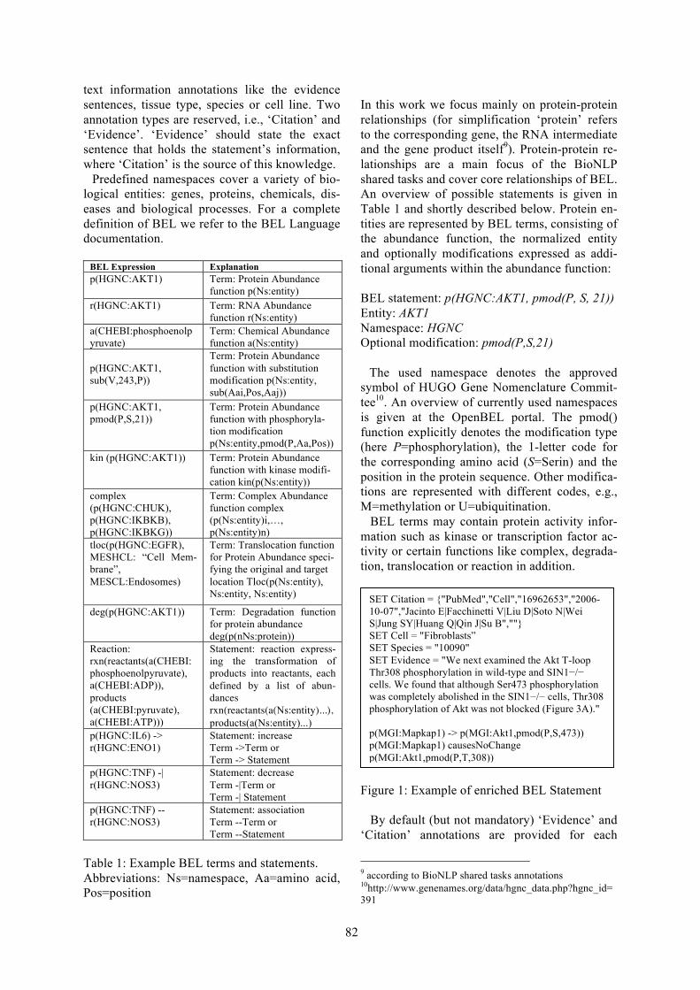
text information annotations like the evidence sentences, tissue type, species or cell line. Two annotation types are reserved, i.e., ‘Citation’ and ‘Evidence’. ‘Evidence’ should state the exact sentence that holds the statement’s information, where ‘Citation’ is the source of this knowledge. Predefined namespaces cover a variety of bio-logical entities: genes, proteins, chemicals, dis-eases and biological processes. For a complete definition of BEL we refer to the BEL Language documentation.
BEL Expression Explanation p(HGNC:AKT1)
Term: Protein Abundance function p(Ns:entity)
r(HGNC:AKT1) Term: RNA Abundance function r(Ns:entity)
a(CHEBI:phosphoenolpyruvate)
Term: Chemical Abundance function a(Ns:entity)
p(HGNC:AKT1, sub(V,243,P))
Term: Protein Abundance function with substitution modification p(Ns:entity, sub(Aai,Pos,Aaj))
p(HGNC:AKT1, pmod(P,S,21))
Term: Protein Abundance function with phosphoryla-tion modification p(Ns:entity,pmod(P,Aa,Pos))
kin (p(HGNC:AKT1)) Term: Protein Abundance function with kinase modifi-cation kin(p(Ns:entity))
complex (p(HGNC:CHUK), p(HGNC:IKBKB), p(HGNC:IKBKG))
Term: Complex Abundance function complex (p(Ns:entity)i,…, p(Ns:entity)n)
tloc(p(HGNC:EGFR), MESHCL: “Cell Mem-brane”, MESCL:Endosomes)
Term: Translocation function for Protein Abundance speci-fying the original and target location Tloc(p(Ns:entity), Ns:entity, Ns:entity)
deg(p(HGNC:AKT1)) Term: Degradation function for protein abundance deg(p(nNs:protein))
Reaction: rxn(reactants(a(CHEBI: phosphoenolpyruvate), a(CHEBI:ADP)), products (a(CHEBI:pyruvate), a(CHEBI:ATP)))
Statement: reaction express-ing the transformation of products into reactants, each defined by a list of abun-dances rxn(reactants(a(Ns:entity)...), products(a(Ns:entity)...)
p(HGNC:IL6) -> r(HGNC:ENO1)
Statement: increase Term ->Term or Term -> Statement
p(HGNC:TNF) -| r(HGNC:NOS3)
Statement: decrease Term -|Term or Term -| Statement
p(HGNC:TNF) --r(HGNC:NOS3)
Statement: association Term --Term or Term --Statement
Table 1: Example BEL terms and statements. Abbreviations: Ns=namespace, Aa=amino acid, Pos=position
In this work we focus mainly on protein-protein relationships (for simplification ‘protein’ refers to the corresponding gene, the RNA intermediate and the gene product itself9). Protein-protein re-lationships are a main focus of the BioNLP shared tasks and cover core relationships of BEL. An overview of possible statements is given in Table 1 and shortly described below. Protein en-tities are represented by BEL terms, consisting of the abundance function, the normalized entity and optionally modifications expressed as addi-tional arguments within the abundance function: BEL statement: p(HGNC:AKT1, pmod(P, S, 21)) Entity: AKT1 Namespace: HGNC Optional modification: pmod(P,S,21)
The used namespace denotes the approved symbol of HUGO Gene Nomenclature Commit-tee10. An overview of currently used namespaces is given at the OpenBEL portal. The pmod() function explicitly denotes the modification type (here P=phosphorylation), the 1-letter code for the corresponding amino acid (S=Serin) and the position in the protein sequence. Other modifica-tions are represented with different codes, e.g., M=methylation or U=ubiquitination. BEL terms may contain protein activity infor-mation such as kinase or transcription factor ac-tivity or certain functions like complex, degrada-tion, translocation or reaction in addition.
Figure 1: Example of enriched BEL Statement By default (but not mandatory) ‘Evidence’ and ‘Citation’ annotations are provided for each
9 according to BioNLP shared tasks annotations 10http://www.genenames.org/data/hgnc_data.php?hgnc_id=391
SET Citation = {"PubMed","Cell","16962653","2006-10-07","Jacinto E|Facchinetti V|Liu D|Soto N|Wei S|Jung SY|Huang Q|Qin J|Su B",""} SET Cell = "Fibroblasts” SET Species = "10090" SET Evidence = "We next examined the Akt T-loop Thr308 phosphorylation in wild-type and SIN1−/− cells. We found that although Ser473 phosphorylation was completely abolished in the SIN1−/− cells, Thr308 phosphorylation of Akt was not blocked (Figure 3A)." p(MGI:Mapkap1) -> p(MGI:Akt1,pmod(P,S,473)) p(MGI:Mapkap1) causesNoChange p(MGI:Akt1,pmod(P,T,308))
82
statement. In case of extraction from literature the reference source and the evidence sentences are given. Alternative evidences may be derived from tables, figures, supplementary material or other knowledge sources. Optionally, the BEL statements can be annotated with specified in-formation about experimental methods, the bio-logical system in which the facts are represented, or even information in which part of the full text the evidence has been found. An example of such a BEL statement from a small sample set at the OpenBEL portal11 is shown in Figure 1. Such detailed information from literature, in combina-tion with the BEL statements, could serve as ide-al source for the generation of training data for text mining purposes to facilitate the develop-ment of future automated extraction algorithms.
4 Analysis of basic concepts in the Bio-NLP shared task annotations
In the main BioNLP shared task (GE12) nine event types are defined (cf Table 2). ‘Gene ex-pression’, ‘Transcription’, ‘Protein catabolism’, ‘Phosphorylation’ and ‘Localization’ are simple events, having one protein as Theme argument.
Event Primary Arg. Second-ary Arg.
Gene Expression Theme(Protein) Transcription Theme(Protein) Protein Catabolism Theme(Protein) Phosphorylation Theme(Protein) Site
Localization Theme(Protein) AtLoc, ToLoc
Binding Theme(Protein)+ Site+ Regulation, Positive Regulation, Nega-tive Regulation
Theme(Protein/Event),Cause(Protein/Event)
Cause, Site, CSite
Table 2: Event types defined in the BioNLP competitions (adapted from (Kim et al., 2012). A ‘+‘ sign indicates multiple occurrences allowed. Events ‘Phosphorylation’ and ‘Localization’ may have additional secondary arguments, like the phosphorylation site or the localization ar-guments ToLoc and AtLoc. ‘Binding’ events can have an arbitrary number of proteins as Themes. Events ‘Positive regulation’, ‘Negative regula-
11 https://github.com/OpenBEL/openbel-framework-resources/blob/master/knowledge/small_corpus.bel 12 https://sites.google.com/site/bionlpst/home/genia-event-extraction-genia
tion’ and ‘Regulation’ are Regulation Events and have a primary Theme argument and an optional Cause argument, both being either a protein or an event. The trigger is always the textual repre-sentation of the entities. Table 3 depicts an ex-ample annotation for the following sentences13: S1) E1-4: “RFLAT-1: a new zinc finger transcription factor that activates RANTES gene expression in T lymphocytes.” S2) E5-9: “In this study we hypothesized that the phosphor-ylation of TRAF2 inhibits binding to the CD40 cytoplasmic domain.”
ID Theme Type Trigger Theme Cause
T1 Protein RFLAT-1
T2 Protein RANTES
E3 Gene
Expression
gene ex-pression
T2
E4 Positive
Regulation
activates E3 T1
T5 Protein TRAF-2
T6 Protein CD40
E7 Phosphorylation phosphor-ylation
T5
E8 Binding binding T6 T5
E9 Negative
Regulation
inhibits E8 E7
Table 3: Example BioNLP 09 shared task anno-tation. The gene/protein entities with the Ids T1, T2, T5, and T6 were already provided. The task was to detect the events E3, E4, E7, E8 and E9.
5 Syntactic mapping from BioNLP an-notation to BEL statements
For mapping of the BEL statements and the out-put of the BioNLP shared tasks systems we com-pared the training data for the GENIA BioNLP task with the BEL statements found in the small corpus at the OpenBEL website. The BioNLP shared task provides no normalization of the en-tities to namespaces. Since we are mainly inter-ested in the transformation of the event, we ig-nore the normalization aspect in the conversion process. For most Shared Task events we could
13 Examples taken from http://www.nactem.ac.uk/tsujii/ GENIA/SharedTask/detail.shtml
83
generate BEL Terms which are summarized with the rule set in Table 4 and Table 5. Standard translation for all protein Themes is protein abundance p(namespace:entity). In a later network generation step within the BEL frame-work RNA abundance and gene abundance are added automatically to the network of statements for all protein abundances. Due to this reason, we only consider RNA or gene abundance if we de-tect strong evidences for those states. For Gene_expression, the protein abundance is only converted to RNA abundance (r(name-space:entity)) if the trigger word is ‘gene expres-sion’.
1.1 GeneExpression(Theme(protein)) à p(Ns:protein) If the GeneExpression trigger word is stemmed to ‘express’
1.2 GeneExpression(Theme(protein)) à r(Ns:protein) For all other GeneExpression trigger words.
2 Transcription(Theme(protein) ) à r(Ns:entity) 3 Phosphorylation(Theme(protein), <Site>) à
p(Ns:protein, <pmod(P,Aa, Pos)>) 4 ProteinCatabolism(Theme(protein))à
deg(p(Ns:protein)) 5.1 Localization(Theme(protein)) à sec (p(Ns:protein))
If the Localization trigger is stemmed to ‘secrete’
5.2 Localization(Theme(protein),AtLoc) à surf(p(Ns:protein)) If the Localization trigger is stemmed to ‘express’ and If AtLoc is ‘cell surface’ or ‘surface’
5.3 Localization(Theme(protein),AtLoc, ToLoc) à tloc (p(Ns:protein),Ns:AtLoc,Ns:ToLoc) In BEL statements it is necessary to have AtLoc and ToLoc; for some cases the missing information can be inferred otherwise artificial location information is given.
6 Binding(Theme(protein)+,Site+) à com-plex(p(ns:protein),+) The site information will be ignored.
Table 4: Rule set 1 to map BioNLP annotations to BEL statements. If the trigger word ‘expression’ is used, both RNA and protein expression might be meant by the authors, hence we keep the protein abun-dance in those cases. Similarly for Transcription, the abundance is changed to RNA abundance. All complexes are translated to protein abun-dance and chemical names are directly translated into abundance (a(ns:chemical names)). Protein modification events such as Phosphorylation can be directly converted to BEL terms. The different
modification events are translated to a single let-ter code in BEL. If the position information is given in the site expression it can directly be converted to the amino acid single letter code (Aa) and the position information (Pos). For the simple events Protein degradation and Binding, the translation is straightforward given their similar representation. The site information of the Binding event is omitted in the BEL state-ment conversion. It would only be included if there is an experiment showing that a mutation of the site would lead to a suppression of the com-plex building. In the case of ‘Localization’, depending on the localisation trigger different BEL functions are possible. Given the localization trigger ‘secrete’ the BEL annotation is converted to the secretion (sec) function. If trigger words ‘surface’ or ‘cell surface’ are identified, the cellSurface (surf) function is assigned. For other Atloc and ToLoc triggers the function translocation (tloc) is used. This function always needs two arguments of location. If one of the arguments (AtLoc or ToLoc) is missing, a general annotation of MESHCL:“Intracellular Space” is proposed as unknown intracellular location.
Activity status like gtp(p(protein)), kin (p(protein)), tscript(p(protein)), cat(p(protein)), phos(p(protein)) are often found in the BEL ex-ample corpus. This information might be partly inferred through the evidence information. In the first example sentence from Table 2, RFLAT-1 might be directly translated into tscript (p(RFLAT-1)). In other cases if a protein phos-phorylates another protein directly, the kin(p(protein)) annotation can be added as well. However, in most cases the information cannot directly be inferred from the sentences (cf. Fig-ure 1). The annotators obviously use their back-ground knowledge to include this information. In the actual status of the Shared Task to BEL con-version we omitted those functions. Looking at the rule-set for transferring Shared-Task events to BEL statements, it is observed that for most events (six out of nine) only BEL terms are generated, i.e., only the left or right hand side of a complete statement. Three rules generate complete BEL statements out of the following events: Regulation, Positive Regula-tion and Negative Regulation. Analysis of the distribution of Events in Shared-Tasked training set (BioNLP ST 2011) reveals that approximate-ly half of the events are Regulation events and
84
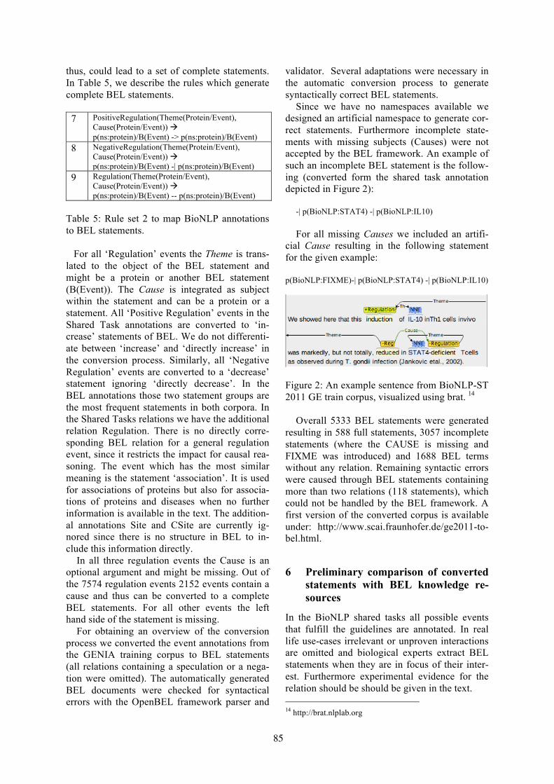
thus, could lead to a set of complete statements. In Table 5, we describe the rules which generate complete BEL statements.
7 PositiveRegulation(Theme(Protein/Event), Cause(Protein/Event)) à p(ns:protein)/B(Event) -> p(ns:protein)/B(Event)
8 NegativeRegulation(Theme(Protein/Event), Cause(Protein/Event)) à p(ns:protein)/B(Event) -| p(ns:protein)/B(Event)
9 Regulation(Theme(Protein/Event), Cause(Protein/Event)) à p(ns:protein)/B(Event) -- p(ns:protein)/B(Event)
Table 5: Rule set 2 to map BioNLP annotations to BEL statements. For all ‘Regulation’ events the Theme is trans-lated to the object of the BEL statement and might be a protein or another BEL statement (B(Event)). The Cause is integrated as subject within the statement and can be a protein or a statement. All ‘Positive Regulation’ events in the Shared Task annotations are converted to ‘in-crease’ statements of BEL. We do not differenti-ate between ‘increase’ and ‘directly increase’ in the conversion process. Similarly, all ‘Negative Regulation’ events are converted to a ‘decrease’ statement ignoring ‘directly decrease’. In the BEL annotations those two statement groups are the most frequent statements in both corpora. In the Shared Tasks relations we have the additional relation Regulation. There is no directly corre-sponding BEL relation for a general regulation event, since it restricts the impact for causal rea-soning. The event which has the most similar meaning is the statement ‘association’. It is used for associations of proteins but also for associa-tions of proteins and diseases when no further information is available in the text. The addition-al annotations Site and CSite are currently ig-nored since there is no structure in BEL to in-clude this information directly.
In all three regulation events the Cause is an optional argument and might be missing. Out of the 7574 regulation events 2152 events contain a cause and thus can be converted to a complete BEL statements. For all other events the left hand side of the statement is missing.
For obtaining an overview of the conversion process we converted the event annotations from the GENIA training corpus to BEL statements (all relations containing a speculation or a nega-tion were omitted). The automatically generated BEL documents were checked for syntactical errors with the OpenBEL framework parser and
validator. Several adaptations were necessary in the automatic conversion process to generate syntactically correct BEL statements.
Since we have no namespaces available we designed an artificial namespace to generate cor-rect statements. Furthermore incomplete state-ments with missing subjects (Causes) were not accepted by the BEL framework. An example of such an incomplete BEL statement is the follow-ing (converted form the shared task annotation depicted in Figure 2):
-| p(BioNLP:STAT4) -| p(BioNLP:IL10) For all missing Causes we included an artifi-
cial Cause resulting in the following statement for the given example:
p(BioNLP:FIXME)-| p(BioNLP:STAT4) -| p(BioNLP:IL10)
Figure 2: An example sentence from BioNLP-ST 2011 GE train corpus, visualized using brat. 14
Overall 5333 BEL statements were generated
resulting in 588 full statements, 3057 incomplete statements (where the CAUSE is missing and FIXME was introduced) and 1688 BEL terms without any relation. Remaining syntactic errors were caused through BEL statements containing more than two relations (118 statements), which could not be handled by the BEL framework. A first version of the converted corpus is available under: http://www.scai.fraunhofer.de/ge2011-to-bel.html.
6 Preliminary comparison of converted statements with BEL knowledge re-sources
In the BioNLP shared tasks all possible events that fulfill the guidelines are annotated. In real life use-cases irrelevant or unproven interactions are omitted and biological experts extract BEL statements when they are in focus of their inter-est. Furthermore experimental evidence for the relation should be should be given in the text. 14 http://brat.nlplab.org
85
In addition biologists are able to do a semantic interpretation of the experimental results and generate inferred statements. To find solutions for semantic interpretation for a number of in-complete statements in the direct conversion for the BioNLP-ST annotations we compared sen-tences such as annotated in figure 2 with evi-dence sentences in the BEL sample set. In the following examples we show how an expert cu-rator conversely infers BEL statements by inter-preting experiment readouts. Example 1: Evidence = "PI 3- kinase/PKCξ, but not PI 3-kinase/Akt signaling pathway, is inhibited in IRS-2-deficient brown adipocytes upon insulin stimulation" p(HGNC:IRS2)-> kinase(p(HGNC:PRKCZ)) p(HGNC:IRS2) causesNoChange kin(p(HGNC:AKT1)) Example 2: Evidence = "transient transfection of primary brown adipo-cytes with a dominant negative form of p21 Ras completely abolished insulin-induced UCP-1-CAT transactivation." p(PFH:"RAS Family") -> (p(HGNC:INS) -> r(HGNC:UCP1)) Example 3: Evidence = "We next examined the Akt T-loop Thr308 phosphorylation in wild-type and SIN1−/− cells. We found that Thr308 phosphorylation was completely abolished in the SIN1−/− cells.” p(MGI:Mapkap1) -> p(MGI:Akt1,pmod(P,T,308)) The examples given above demonstrate a standard experimental setting. In most cases the functionality of a gene is abolished and the effect (e.g. increase, decrease or no effect) on the cor-responding interaction targets is observed. Some-times, observed effects are compared to cell sys-tems where the normal form (wild type or con-trol) is transfected as well (cf. Example 3). All examples share the readout: The BEL statement is not describing the experiment (given in the sentence), but the observed implication inferred from the experiment (cf. Example 2). Instead of encoding that a dysfunctional p21 RAS leads to an abolishment of insulin induced UCP1 transactivation, the final BEL statement represents the resulting implication, i.e. wild-type p21 RAS increases INS, which subsequent-ly increases UCP1: p(PFH:"RAS Family") -> (p(HGNC:INS) -> r(HGNC:UCP1))
Similarly, in Example 3 from the abolishment of a function, the converse argument is derived, i.e. Mapkap 1 increases the phosphorylation of Akt1 at T308. This example shows another main issue in deriving BEL statements: two or more sen-tences are needed to get all information neces-sary to create a valid BEL statement. Human cu-rators use multiple sentences as evidence and do additional interpretation of the provided infor-mation. In Example 3, the AKT phosphorylation is given in the first sentence and the phosphory-lation event is given in the following sentence only in referring to the site and not to the protein. BioNLP-ST already includes annotation span-ning several sentences but interpretation and merging of those annotations is not trivial. To complete such statements two different relations have to be combined and that is true for many modification relations. Especially in the case of phosphorylation, which is a regular activating signal in kinase pathways, we need solutions in-cluding information from different sentences. The BEL corpus has a high number of phosphor-ylation events and can serve as a base for the generation of further training data. Another commonly observed experiment uses luciferase and CAT vectors. Those systems are used to analyze transcriptional activity of pro-moters in dependence of stimuli. The result of such an experiment is oftentimes given only as a relation to CAT or luciferase like in the follow-ing example: Example 4: Evidence = "introduction of miR-145, but not miR-143, with the luciferase vector in Cos cells resulted in relief of the repression and an ~150-fold increase in luciferase activi-ty compared to the CMV-luciferase- Myocd 3' UTR-luciferase vector alone.” miR(HGNC:MIR145) -> p(HGNC:MYOCD) miR(HGNC:MIR143) causesNoChange p(HGNC:MYOCD) BioNLP shared task annotation would capture positive regulation of luciferase activity with the cause miR-145. The derived statement however does not state an abundance function for lucifer-ase but the originally tested protein (indirectly via its promotor) i.e., Myocd. Here, the inserted promoter information is given at the end of the sentence, although it is often provided in a sepa-rate sentence. The second BEL statement in Example 4 pro-vides another relation type, which is not directly captured by the shared task annotations. Nega-
86
tive results are annotated in BEL statements with the relation causesNoChange and are valuable relations in causal reasoning. They might be in-terpreted using the negation annotation in shared task to capture this type of event. Those examples are only a few out of numer-ous others. For the development of suitable sys-tems, annotated training corpora are crucial. The BEL documents might be a good starting point to generate further training corpora containing a high number of such evidence examples. How-ever, the conversion of the BEL statements to BioNLP shared task annotation is not trivial, since position information is completely missing. Nevertheless, it might reduce the annotation ef-fort, give good examples and serve as a basis for biological interpretation of the relations. For ini-tial automatic systems it might be even sufficient to offer such experimental evidence sentences in addition to the extracted relations to users.
7 Discussion and Conclusions
Generally, a syntactic conversion of BioNLP shared task annotations to BEL terms and state-ments is possible and in most cases without in-formation loss. Tools developed or adapted for the BioNLP shared task are principally suited for the generation of causal BEL networks. Howev-er, the analysis of the automatically converted BEL statements from the BioNLP shared tasks shows that in a number of cases incomplete BEL statements were generated. Part of the reason is the need for an additional interpretation layer that would help in generating biologically mean-ingful statements. Another reason for the failure to extract full statements is the distribution of the relation over more than one sentence. The properties of BEL statements and the addi-tional information coded in the BEL documents represent a valuable resource for generating fur-ther training data for the development of more real-world oriented systems. Unfortunately, the information of the BEL documents cannot direct-ly be converted back to textual annotation. The main reason is that the position information of entities within the relation is missing. Reverse engineering is also challenging because the trig-ger words are not given. Furthermore, normaliza-tion to namespaces used in BEL statements makes the direct mapping difficult. Nevertheless, the text mining community can learn from the BEL documents what are relevant
statements for causal reasoning and from which evidence sentences humans extract the infor-mation. The example BEL statements given show that humans use a number of experimental systems such as inactive versions of proteins or reporter genes to prove existing relationships. It might be a realistic task to use BEL documents as a starting point to generate training corpora for the automatic classification of such sentences and for information extraction systems to extract relations from those sentences. For some rela-tions like the phosphorylation or the reporter genes, we might be even able to extract relations over sentences when enough training data is available. Another problem not tackled by the BioNLP shared tasks is the mapping to the name spaces. There are already systems available combining BioNLP based relation extraction systems and named entity recognition (NER) systems allow-ing for normalization and (eg. Björne et al., 2012 and Van Landeghem et al., 2013). Future sys-tems have to combine relation extraction and NER systems allowing for normalization. Gene and protein names have already been in the focus of the BioCreative assessments during the last years (cf. Morgan et al., 2008 and Lu et al., 2011). In addition, chemical entities are coming more and more into the focus of the community (e.g., in the BioCreative 2013 task15). In the ex-amples from the BEL corpus we see additional problems coming from the area of engineered genes. Name variants are often used (e.g., Sin-/- or CMV-luciferase- Myocd 3' UTR-luciferase), which causes further problems in the normaliza-tion task. Bridging the BEL and the BioNLP-ST com-munity offers benefits for both sides. The Bio-NLP shared tasks are a considerable start for the automatic generation of causal networks. Moreo-ver, already available BEL documents can sup-port the generation of the huge amount of addi-tional training data, which is necessary for fur-ther relation extraction development.
15 http://www.biocreative.org/events/biocreative-iv/CFP/
87
Acknowledgments
We would like to thank Natalie Catlett and Ted Slater of Selventa for providing their time and expertise in helping us understand BEL. We acknowledge support of our research from Philip Morris International.
References Jari Björne, Sofie Van Landeghem, Sampo Pyysalo,
Tomoko Ohta, Filip Ginter, Yves Van de Peer, Sophia Ananiadou and Tapio Salakoski. 2012. PubMed-Scale Event Extraction for Post-Translational Modifications, Epigenetics and Pro-tein Structural Relations. Proceedings of BioNLP 2012, 82-90
Leonid Chindelevitch, Daniel Ziemek, Ahmed Enaye-tallah, Ranjit Randhawa, Ben Sidders, Christoph Brockel and Enoch Huang. 2012. Causal reason-ing on biological networks: interpreting transcrip-tional changes. Bioinformatics. 28(8):1114-21.
Emek Demir et al. 2010. The BioPAX community standard for pathway data sharing. Nature bio-technology , 28(9):935–942.
Chia-Ling Huang, John Lamb, Leonid Chindelevitch, Jarek Kostrowicki, Justin Guinney, Charles DeLisi and Daniel Ziemek. 2012. Correlation set analysis: detecting active regulators in disease populations using prior causal knowledge. BMC Bioinformat-ics. 2012 13:46.
Michael Hucka et al. 2003. The systems biology markup language (SBML): a medium for re-presentation and exchange of biochemical network models. Bioinformatics , 19(4):524–531.
Jim-Dong Kim, Ngan Nguyen, Yue Wang, Jun’ichi Tsujii, Toshihisa Takagi and Akinori Yonezawa. 2012. The Genia Event and Protein Coreference tasks of the BioNLP Shared Task 2011. BMC Bio-informatics. 13 Suppl 11:S1.
Zhiyong Lu et al. 2011. The gene normalization task in BioCreative III. BMC Bioinformatics , 12(Suppl 8):S2.
Alexander A Morgan et al. 2008. Overview of Bio-Creative II gene normalization. Genome Biol. 9 Suppl 2:S3.
Tomoko Ohta,_ Sampo Pyysalo, Sophia Ananiadou and Jun’ichi Tsujii. 2011. Pathway Curation Sup-port as an Information Extraction Task. Procee-dings of the Fourth International Symposium on Languages in Biology and Medicine (LBM 2011).
Tomoko Ohta, Sampo Pyysalo and_Jun’ichi Tsujii. 2011. From Pathways to Biomolecular Events: Opportunities and Challenges. Proceedings of the 2011 Workshop on Biomedical Natural Language Processing , ACL-HLT 2011, pages 105–113.
Walter K. Schlage, et al. 2011. A computable cellular stress network model for non-diseased pulmonary and cardiovascular tissue. BMC Syst Biol. 5:168.
Ted Slater and Diana H. Song. 2012. Saved by the
BEL: ringing in a common language for the life sciences. Drug Discovery World Fall 2012 75:80
Selventa 2012 Reverse Causal Reasoning Methods Whitepaper
http://www.selventa.com/publications/white-papers
Sofia Van Landeghem, Jari Björne, Chih H Wei, Kai Hakala , Sampo Pyysalo, Sophia Ananiadou,
Hung-Yu Kao, Zhiyong Lu, Tapio Salakoski, Yves Van de Peer, and Filip Ginter. 2013. Large-Scale Event Extraction from Literature with Multi-Level Gene Normalization. PLoS ONE 8(4): e55814.
88
Proceedings of the 2013 Workshop on Biomedical Natural Language Processing (BioNLP 2013), pages 89–97,Sofia, Bulgaria, August 4-9 2013. c©2013 Association for Computational Linguistics
Exploring word class n-grams to measurelanguage development in children
Gabriela Ramırez de la Rosa and Thamar SolorioUniversity of Alabama at Birmingham
Birmingham, AL 35294, USAgabyrr,[email protected]
Manuel Montes-y-GomezINAOE
Sta. Maria Tonantzintla, Puebla, [email protected]
Yang LiuThe University of Texas at Dallas
Richardson, TX 75080, [email protected]
Aquiles IglesiasTemple University
Philadelphia, PA 19140, [email protected]
Lisa Bedore and Elizabeth PenaThe University of Texas at Austin
Austin, TX 78712, USAlbedore,[email protected]
Abstract
We present a set of new measures designedto reveal latent information of languageuse in children at the lexico-syntacticlevel. We used these metrics to analyzelinguistic patterns in spontaneous narra-tives from children developing typicallyand children identified as having a lan-guage impairment. We observed signif-icant differences in the z-scores of bothpopulations for most of the metrics. Thesefindings suggest we can use these metricsto aid in the task of language assessmentin children.
1 Introduction
The analysis of spontaneous language samples isan important task across a variety of fields. For in-stance, in language assessment this task can helpto extract information regarding language profi-ciency (e.g. is the child typically developing orlanguage impaired). In second language acqui-sition, language samples can help determine ifa child’s proficiency is similar to that of nativespeakers.
In recent years, we have started seeing a grow-ing interest in the exploration of NLP techniquesfor the analysis of language samples in the clinicalsetting. For example, Sahakian and Snyder (2012)
propose a set of linguistic measures for age pre-diction in children that combines three traditionalmeasures from language assessment with a set offive data-driven measures from language samplesof 7 children. A common theme in this emerg-ing line of research is the study of the syntax inthose language samples. For instance, to annotatedata to be used in the study of language develop-ment (Sagae et al., 2005), or to build models tomap utterances to their meaning, similar to whatchildren do during the language acquisition stage(Kwiatkowski et al., 2012). In addition, languagesamples are also used for neurological assessment,as for example in (Roark et al., 2007; Roark etal., 2011) where they explored features such asYngve and Frazier scores, together with featuresderived from automated parse trees to model syn-tactic complexity and surprisal. Similar featuresare used in the classification of language samplesto discriminate between children developing typ-ically and children suffering from autism or lan-guage impairment (Prud’hommeaux et al., 2011).In a similar line of research, machine learning andfeatures inspired by NLP have been explored forthe prediction of language status in bilingual chil-dren (Gabani et al., 2009; Solorio et al., 2011).More recent work has looked at the feasibility ofscoring coherence in story narratives (Hassanali etal., 2012a) and also on the inclusion of coherence
89
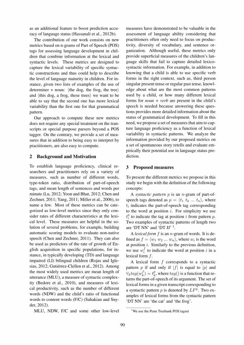
as an additional feature to boost prediction accu-racy of language status (Hassanali et al., 2012b).
The contribution of our work consists on newmetrics based on n-grams of Part of Speech (POS)tags for assessing language development in chil-dren that combine information at the lexical andsyntactic levels. These metrics are designed tocapture the lexical variability of specific syntac-tic constructions and thus could help to describethe level of language maturity in children. For in-stance, given two lists of examples of the use ofdeterminer + noun: 〈the dog, the frog, the tree〉and 〈this dog, a frog, these trees〉 we want to beable to say that the second one has more lexicalvariability than the first one for that grammaticalpattern.
Our approach to compute these new metricsdoes not require any special treatment on the tran-scripts or special purpose parsers beyond a POStagger. On the contrary, we provide a set of mea-sures that in addition to being easy to interpret bypractitioners, are also easy to compute.
2 Background and Motivation
To establish language proficiency, clinical re-searchers and practitioners rely on a variety ofmeasures, such as number of different words,type-token ratio, distribution of part-of-speechtags, and mean length of sentences and words perminute (Lu, 2012; Yoon and Bhat, 2012; Chen andZechner, 2011; Yang, 2011; Miller et al., 2006), toname a few. Most of these metrics can be cate-gorized as low-level metrics since they only con-sider rates of different characteristics at the lexi-cal level. These measures are helpful in the so-lution of several problems, for example, buildingautomatic scoring models to evaluate non-nativespeech (Chen and Zechner, 2011). They can alsobe used as predictors of the rate of growth of En-glish acquisition in specific populations, for in-stance, in typically developing (TD) and languageimpaired (LI) bilingual children (Rojas and Igle-sias, 2012; Gutierrez-Clellen et al., 2012). Amongthe most widely used metrics are mean length ofutterance (MLU), a measure of syntactic complex-ity (Bedore et al., 2010), and measures of lexi-cal productivity, such as the number of differentwords (NDW) and the child’s ratio of functionalwords to content words (F/C) (Sahakian and Sny-der, 2012).
MLU, NDW, F/C and some other low-level
measures have demonstrated to be valuable in theassessment of language ability considering thatpractitioners often only need to focus on produc-tivity, diversity of vocabulary, and sentence or-ganization. Although useful, these metrics onlyprovide superficial measures of the children’s lan-guage skills that fail to capture detailed lexico-syntactic information. For example, in addition toknowing that a child is able to use specific verbforms in the right context, such as, third personsingular present tense or regular past tense, knowl-edge about what are the most common patternsused by a child, or how many different lexicalforms for noun + verb are present in the child’sspeech is needed because answering these ques-tions provides more detailed information about thestatus of grammatical development. To fill in thisneed, we propose a set of measures that aim to cap-ture language proficiency as a function of lexicalvariability in syntactic patterns. We analyze theinformation provided by our proposed metrics ona set of spontaneous story retells and evaluate em-pirically their potential use in language status pre-diction.
3 Proposed measures
To present the different metrics we propose in thisstudy we begin with the definition of the followingconcepts:
A syntactic pattern p is an n-gram of part-of-speech tags denoted as p = 〈t1 t2 ... tn〉, whereti indicates the part-of-speech tag correspondingto the word at position i. For simplicity we usetpi to indicate the tag at position i from pattern p.Two examples of syntactic patterns of length twoare ‘DT NN’ and ‘DT JJ’ 1.
A lexical form f is an n-gram of words. It is de-fined as f = 〈w1 w2 ... wn〉, where wi is the wordat position i. Similarly to the previous definition,we use wf
i to indicate the word at position i in alexical form f .
A lexical form f corresponds to a syntacticpattern p if and only if |f | is equal to |p| and∀ktag(wf
k ) = tpk, where tag() is a function that re-turns the part-of-speech of its argument. The set oflexical forms in a given transcript corresponding toa syntactic pattern p is denoted by LF p. Two ex-amples of lexical forms from the syntactic pattern‘DT NN’ are ‘the cat’ and ‘the frog’.
1We use the Penn Treebank POS tagset
90
DT the (62), a (17), all (8), no(2), that (1)NN frog (16), boy(7), dog (6), boat (4), name (3), place (2), house (2), water (2), rabbit (2), noise (2), stick (1), tree
(1), bye(1), floor (1), um (1), baby (1), forest (1), room (1), foot (1), rock (1), squirrel (1), back (1), rabb (1),card (1), one (1), present (1), dress (1), box (1), family (1)
VBD saw (7), dropped (4), said (4), started (4), looked (3), kicked (3), called (3), found (2), took (2), got (2), jumped(2), heard (2), thought (1), turned (1), fell (1), waked (1), stood (1), wa (1), touched (1), told (1), scared (1), tur(1), haded (1), opened (1), shh (1)
DT NN the frog (3), the dog (2), the place (2), the water (2), the boat (2), a noise (2), the forest (1), the rock (1), a tree(1), a present (1), a um (1), the card (1), the box (1), the rabb (1), the floor (1), the back (1), no one (1)
DT VBD all started (2), all heard (1)
Table 1: Example of 5 syntactic patterns with their lists of lexical forms and the number of repetitionsof each of them. This information corresponds to an excerpt of an example transcript. DT is the part-of-speech tag for determiner, NN for noun, and VBD for verb in past tense.
The bag-of-words associated to a syntactic pat-tern p is denoted as W p. This set is composedof all the words from the lexical forms that corre-spond to the syntactic pattern p. It is formally de-fined as follows: W p = {w|w ∈ f, f ∈ LF p}.For example, the bag-of-words of the syntacticpattern ‘DT NN’ with lexical forms ‘the cat’ and‘the frog’ is {the, cat, frog}.
Table 1 shows five syntactic patterns of a tran-script’s fragment. For each syntactic pattern in thetranscript we show the list of its lexical forms andtheir frequency. We will use this example in thedescription of the measures in the following sub-sections.
3.1 Number of different lexical forms(NDLF)
Analogous to the number of different words(NDW), where words in the transcript are consid-ered atomic units, we propose a metric where theatomic units are lexical forms. Then, we measurethe number of different lexical forms used for eachsyntactic pattern in the transcript. Formally, givena syntactic pattern p and its set of lexical formsLF p, the number of different lexical forms is com-puted as follows:
NDLF(p) = |LF p| (1)
This measure gives information about the num-ber of different ways the child can combine wordsin order to construct a fragment of a speech thatcorresponds to a specific grammatical pattern. Re-search in language assessment has shown thatwhen children are in the early acquisition stagesof certain grammatical constructions they will usethe patterns as “fixed expressions”. As childrenmaster these constructions they are able to usethese grammatical devices in different contexts,
but also with different surface forms. Thereby, wecould use this measure to discriminate the syntac-tic patterns the child has better command of fromthose that might still be problematic and used in-frequently or with a limited combination of sur-face forms. For example, from the informationon Table 1 we see that NDLF(DT NN) = 17, andNDLF(DT VBD) = 2. This seems to indicate thatthe child has a better command of the grammaticalconstruction determiner + noun (DT NN) and canthus produce more different lexical forms of thispattern than determiner + verb (DT + VBD). Butalso, we may use this measure to identify rare pat-terns, that are unlikely to be found in a typicallydeveloping population.
3.2 Lexical forms distribution (LFdist)Following the idea of lexical forms as atomicunits, NDLF allows to know the different lexicalforms present in the transcripts. But we do notknow the distribution of use of each lexical formfor a specific syntactic pattern. In other words,NDLF tells us the different surface forms observedfor each syntactic pattern, but it does not measurethe frequency of use of each of these lexical forms,nor whether each of these forms are used at similarrates. We propose to use LFdist to provide infor-mation about the distribution of use for LF p, theset of lexical forms observed for the syntactic pat-tern p. We believe that uniform distributions canbe indicative of syntactic structures that the childhas mastered, while uneven distributions can re-veal structures that the child has only memorized(i.e. the child uses a fixed and small set of lex-ical forms). To measure this distribution we usethe entropy of each syntactic pattern. In particu-lar, given a syntactic pattern p and its set of lexicalforms LF p, the lexical form distribution is com-puted as follows:
91
LFdist(p) = −∑
fi∈LF p
prob(fi) log prob(fi)
(2)where
prob(fi) =count(fi)∑
fk∈LF p count(fk)(3)
and count() is a function that returns the fre-quency of its argument. Larger values of LFdistindicate a greater difficulty in the prediction ofthe lexical form that is being used under a spe-cific grammatical pattern. For instance, in the ex-ample of Table 1, LFdist(DT VBD) = 0.91 andLFdist(DT NN) = 3.97. This indicates that thedistribution in the use of lexical forms for deter-miner + noun is more uniform than the use oflexical forms for determiner + verb, which im-plies that for determiner + verb there are somelexical forms that are more frequently used thanothers2. Syntactic patterns with small values ofLFdist could flag grammatical constructions thechild does not feel comfortable manipulating andthus might still be in the acquisition stage of lan-guage learning.
3.3 Lexical variation (LEX)
Until now we are considering lexical forms asatomic units. This could lead to overestimatingthe real lexical richness in the sample, in particu-lar for syntactic patterns of length greater than 1.To illustrate this consider the syntactic pattern p =〈DT NN〉 and suppose we have the following setof lexical forms for p = {‘the frog’, ‘a frog’, ‘adog’, ‘the dog’}. The value for NDLF (p) = 4.But how many of these eight words are in fact dif-ferent? That is the type of distinction we want tomake with the next proposed measure: LEX, thatis also an adaptation of type-token ratio (Lu, 2012)used in the area of communication disorders butcomputed over each grammatical pattern. For thisexample, we want to be able to find that the lex-ical variation of 〈DT NN〉 is 0.5 (because thereare only four different words out of eight). For-mally, given a syntactic pattern p, its set of lexicalforms LF p, and the bag-of-words W p, the lexicalvariation is defined as shown in Equation 4.
2We recognize that this is an oversimplification of the en-tropy measure since the number of outcomes will most likelybe different for each syntactic pattern.
LEX(p) =|W p||LF p| ∗ n
(4)
Note that |LF p| = NDLF(p), and n is thelength of the syntactic pattern p. In Table 1 the lex-ical variation of the pattern ‘determiner + noun’(DT+NN) is equal to 0.58 ( 20
17∗2 ), and for deter-miner + verb (DT+VBD) is equal to 0.75 ( 3
2∗2 ).That means 58% of total words used under the pat-tern ‘DT+NN’ are different, in comparison withthe 75% for ‘DT+VBD’. In general, the closer thevalue of LEX is to 1, there is less overlap betweenthe words in the lexical forms for that pattern.Our hypothesis behind this measure is that for thesame syntactic pattern TD children may have lessoverlap of words than children with LI, e.g. lessoverlap indicates the use of a more diverse set ofwords.
3.4 Lexical use of syntactic knowledge(LexSyn)
With LEX we hope to accomplish the character-ization of lexical richness of syntactic patternsassuming that each part-of-speech has a similarnumber of possible lexical forms. We assume aswell that less overlap in the words used for thesame grammatical pattern represents a more devel-oped language than that with more overlap. How-ever the definition of LEX overlooks a well knownfact about language: different word classes havea different range of possibilities as their lexicalforms. Consider open class items, such as nounsand verbs, where the lexicon is large and keepsgrowing. In contrast, closed class items, such asprepositions and determiners are fixed and have avery small number of lexical forms. Therefore itseems unfair to assign equal weight to the overlapof words for these different classes. To accountfor this phenomenon, we propose a new measurethat includes the information about the syntacticknowledge that the child shows for each part ofspeech. That is, we weigh the level of overlapfor specific grammatical constructions accordingto the lexicon for the specific word classes in-volved. Since we limit our analysis to the languagesample at hand, we define the ceiling of the lexi-cal richness of a specific word class to be the to-tal number of different surface forms found in thetranscript. In particular, given a syntactic patternp = 〈t1 t2 ... tn〉, with its set of lexical formsLF p, the lexical use of syntactic knowledge is de-fined as:
92

LexSyn(p) =1
n
n∑i=1
|wfi |f ∈ LF p|NDLF(tpi )
(5)
where the numerator is the size of the set ofwords in the i-th position in all the lexical forms.Note that this measure does not make sense forsyntactic patterns of length < 2. Instead, syn-tactic patterns of length 1 were used to identifythe syntactic knowledge of the child by using theNDLF of each POS in p. In the example of Ta-ble 1, LexSyn(DT NN) = 0.59. This value corre-sponds to the sum of the number of different de-terminers used in position 1 for LF p divided bythe total number of different determiners that thischild produced in the sample (for this case, thenumber of determiners that this child produced isgiven by NDLF(DT), that is 5), plus the numberof different nouns used under this syntactic pat-tern over the total number of nouns produced bythe child (NDLF(NN)=29). The complete calcula-tion of LexSyn(DT NN) = 1
2 ∗(35 + 17
29) = 0.59.This contrasts with the value of LexSyn for the pat-tern ‘determiner + verb’, LexSyn(DT VBD) =12 ∗ (
15 + 2
25) = 0.14 that seems to indicate that thechild has more experience combining determinersand nouns than determiners and verbs. Perhapsthis child has had limited exposure to other pat-terns combining determiner and verb, or this pat-tern is at a less mature stage in the linguistic reper-toire of the child.
Children with LI tend to exhibit a less devel-oped command of syntax than their TD cohorts.Syntactic patterns with large values of LexSynshow a high versatility in the use of those syntacticpatterns. However, since the syntactic reference istaken from the same child, this versatility is rela-tive only to what is observed in that single tran-script. For instance, suppose that the total num-ber of different determiners observed in the child’stranscript is 1. Then any time the child uses thatdeterminer in a syntactic pattern, the knowledge ofthis class, according to our metric, will be 100%,which is correct, but this might not be enough todetermine if the syntactic knowledge of the childfor this grammatical class corresponds to age ex-pectations for a typically developing child. In or-der to improve the measurement of the lexical useof syntactic knowledge we propose the measureLexSynEx, that instead of using the informationof the same child to define the coverage of use fora specific word class, it uses the information ob-
served for a held out set of transcripts from TDchildren. This variation allows the option of mov-ing the point of reference to a specific cohort, ac-cording to what is needed.
4 Data set
The data used in this research is part of an ongoingstudy of language impairment in Spanish-Englishspeaking children (Pena et al., 2003). From thisstudy we used a set of 175 children with a meanage of about 70 months. Language status of thesechildren was determined via expert judgment bythree bilingual certified speech-language pathol-ogists. At the end of the data collection period,the experts reviewed child records in both lan-guages including language samples, tests proto-cols, and parent and teacher questionnaire data.They made independent judgments about chil-dren’s lexical, morphosyntactic, and narrative per-formance in each language. Finally, they made anoverall judgment about children’s language abil-ity using a 6 point scale (severely language im-paired to above normal impairment). If at least twoexaminers rated children’s language ability withmild, moderate or severe impairment they were as-signed to the LI group. Percent agreement amongthe three examiners was 90%. As a result of thisprocess, 20 children were identified by the clinicalresearchers as having LI, while the remaining 155were identified as typically developing (TD).
The transcripts were gathered following stan-dard procedures for collection of spontaneous lan-guage samples in the field of communication dis-orders. Using a wordless picture book, the chil-dren were asked to narrate the story. The twobooks used were ‘A boy, a dog, and a frog’ (Mayer,1967) and ‘Frog, where are you?’ (Mayer, 1969).For each child in the sample, 4 transcripts of storynarratives were collected, 2 in each language. Inthis study we use only the transcripts where En-glish was the target language.
5 Procedure
The purpose of the following analysis is to inves-tigate the different aspects in the child’s languagethat can be revealed by the proposed metrics. Allour measures are based on POS tags. We used theCharniak parser (Charniak, 2000) to generate thePOS tags of the transcripts. For all the results re-ported here we removed the utterances from theinterrogators and use all utterances by the chil-
93
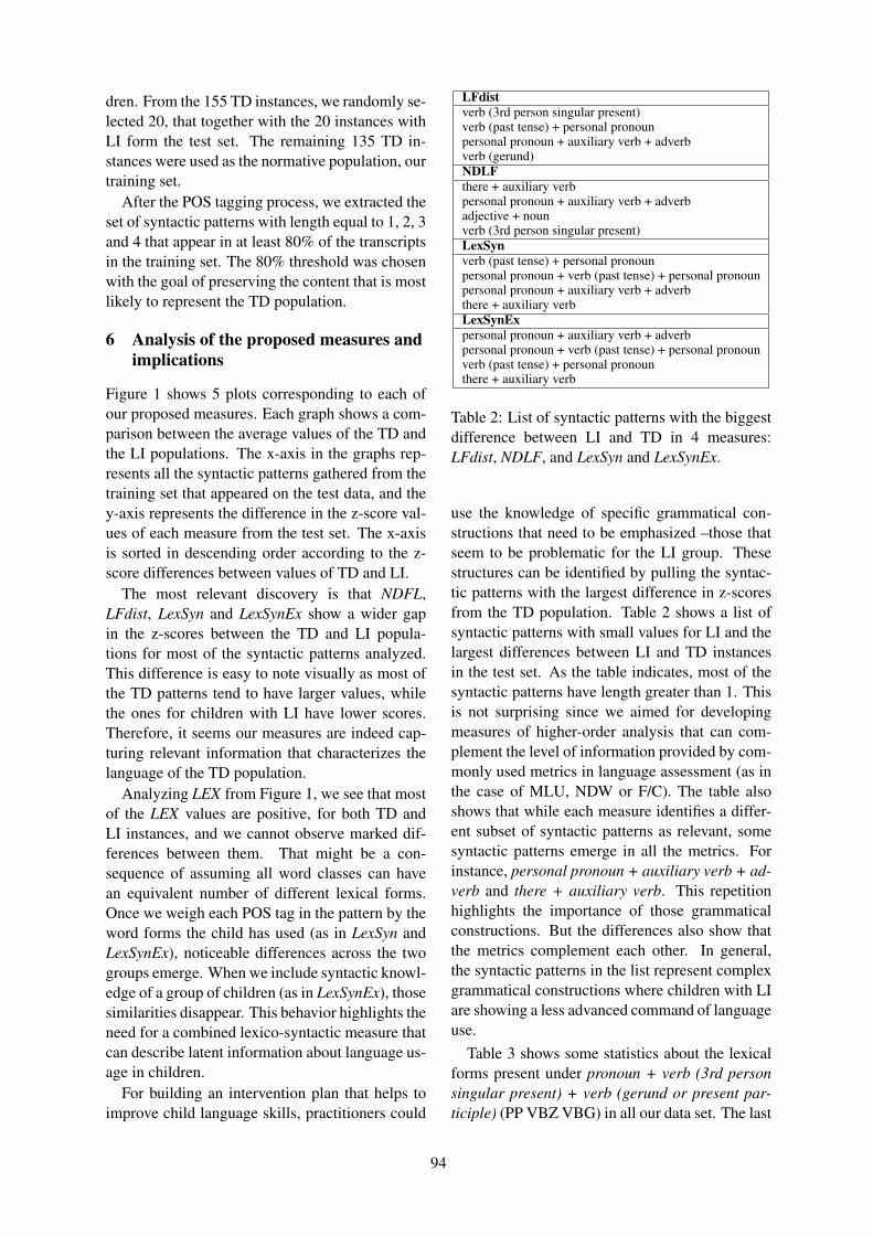
dren. From the 155 TD instances, we randomly se-lected 20, that together with the 20 instances withLI form the test set. The remaining 135 TD in-stances were used as the normative population, ourtraining set.
After the POS tagging process, we extracted theset of syntactic patterns with length equal to 1, 2, 3and 4 that appear in at least 80% of the transcriptsin the training set. The 80% threshold was chosenwith the goal of preserving the content that is mostlikely to represent the TD population.
6 Analysis of the proposed measures andimplications
Figure 1 shows 5 plots corresponding to each ofour proposed measures. Each graph shows a com-parison between the average values of the TD andthe LI populations. The x-axis in the graphs rep-resents all the syntactic patterns gathered from thetraining set that appeared on the test data, and they-axis represents the difference in the z-score val-ues of each measure from the test set. The x-axisis sorted in descending order according to the z-score differences between values of TD and LI.
The most relevant discovery is that NDFL,LFdist, LexSyn and LexSynEx show a wider gapin the z-scores between the TD and LI popula-tions for most of the syntactic patterns analyzed.This difference is easy to note visually as most ofthe TD patterns tend to have larger values, whilethe ones for children with LI have lower scores.Therefore, it seems our measures are indeed cap-turing relevant information that characterizes thelanguage of the TD population.
Analyzing LEX from Figure 1, we see that mostof the LEX values are positive, for both TD andLI instances, and we cannot observe marked dif-ferences between them. That might be a con-sequence of assuming all word classes can havean equivalent number of different lexical forms.Once we weigh each POS tag in the pattern by theword forms the child has used (as in LexSyn andLexSynEx), noticeable differences across the twogroups emerge. When we include syntactic knowl-edge of a group of children (as in LexSynEx), thosesimilarities disappear. This behavior highlights theneed for a combined lexico-syntactic measure thatcan describe latent information about language us-age in children.
For building an intervention plan that helps toimprove child language skills, practitioners could
LFdistverb (3rd person singular present)verb (past tense) + personal pronounpersonal pronoun + auxiliary verb + adverbverb (gerund)NDLFthere + auxiliary verbpersonal pronoun + auxiliary verb + adverbadjective + nounverb (3rd person singular present)LexSynverb (past tense) + personal pronounpersonal pronoun + verb (past tense) + personal pronounpersonal pronoun + auxiliary verb + adverbthere + auxiliary verbLexSynExpersonal pronoun + auxiliary verb + adverbpersonal pronoun + verb (past tense) + personal pronounverb (past tense) + personal pronounthere + auxiliary verb
Table 2: List of syntactic patterns with the biggestdifference between LI and TD in 4 measures:LFdist, NDLF, and LexSyn and LexSynEx.
use the knowledge of specific grammatical con-structions that need to be emphasized –those thatseem to be problematic for the LI group. Thesestructures can be identified by pulling the syntac-tic patterns with the largest difference in z-scoresfrom the TD population. Table 2 shows a list ofsyntactic patterns with small values for LI and thelargest differences between LI and TD instancesin the test set. As the table indicates, most of thesyntactic patterns have length greater than 1. Thisis not surprising since we aimed for developingmeasures of higher-order analysis that can com-plement the level of information provided by com-monly used metrics in language assessment (as inthe case of MLU, NDW or F/C). The table alsoshows that while each measure identifies a differ-ent subset of syntactic patterns as relevant, somesyntactic patterns emerge in all the metrics. Forinstance, personal pronoun + auxiliary verb + ad-verb and there + auxiliary verb. This repetitionhighlights the importance of those grammaticalconstructions. But the differences also show thatthe metrics complement each other. In general,the syntactic patterns in the list represent complexgrammatical constructions where children with LIare showing a less advanced command of languageuse.
Table 3 shows some statistics about the lexicalforms present under pronoun + verb (3rd personsingular present) + verb (gerund or present par-ticiple) (PP VBZ VBG) in all our data set. The last
94
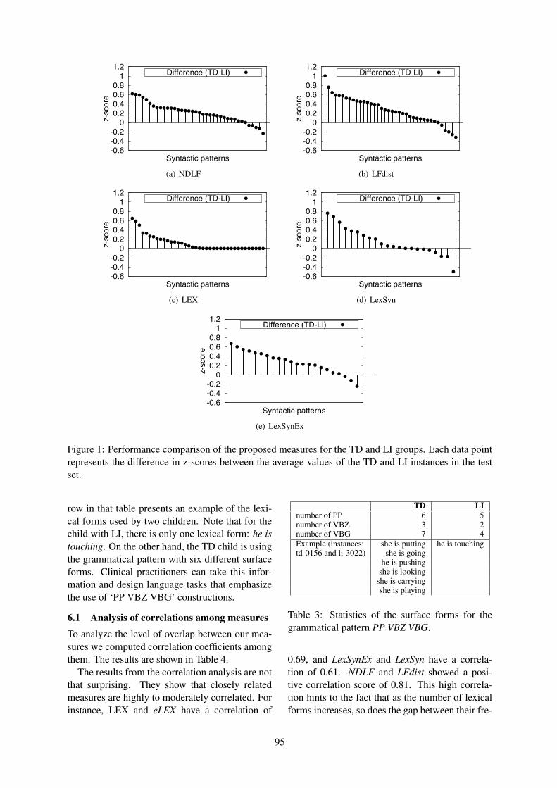
-0.6-0.4-0.2
0 0.2 0.4 0.6 0.8
1 1.2
z-sc
ore
Syntactic patterns
Difference (TD-LI)
(a) NDLF
-0.6-0.4-0.2
0 0.2 0.4 0.6 0.8
1 1.2
z-sc
ore
Syntactic patterns
Difference (TD-LI)
(b) LFdist
-0.6-0.4-0.2
0 0.2 0.4 0.6 0.8
1 1.2
z-sc
ore
Syntactic patterns
Difference (TD-LI)
(c) LEX
-0.6-0.4-0.2
0 0.2 0.4 0.6 0.8
1 1.2
z-sc
ore
Syntactic patterns
Difference (TD-LI)
(d) LexSyn
-0.6-0.4-0.2
0 0.2 0.4 0.6 0.8
1 1.2
z-sc
ore
Syntactic patterns
Difference (TD-LI)
(e) LexSynEx
Figure 1: Performance comparison of the proposed measures for the TD and LI groups. Each data pointrepresents the difference in z-scores between the average values of the TD and LI instances in the testset.
row in that table presents an example of the lexi-cal forms used by two children. Note that for thechild with LI, there is only one lexical form: he istouching. On the other hand, the TD child is usingthe grammatical pattern with six different surfaceforms. Clinical practitioners can take this infor-mation and design language tasks that emphasizethe use of ‘PP VBZ VBG’ constructions.
6.1 Analysis of correlations among measuresTo analyze the level of overlap between our mea-sures we computed correlation coefficients amongthem. The results are shown in Table 4.
The results from the correlation analysis are notthat surprising. They show that closely relatedmeasures are highly to moderately correlated. Forinstance, LEX and eLEX have a correlation of
TD LInumber of PP 6 5number of VBZ 3 2number of VBG 7 4Example (instances: she is putting he is touchingtd-0156 and li-3022) she is going
he is pushingshe is looking
she is carryingshe is playing
Table 3: Statistics of the surface forms for thegrammatical pattern PP VBZ VBG.
0.69, and LexSynEx and LexSyn have a correla-tion of 0.61. NDLF and LFdist showed a posi-tive correlation score of 0.81. This high correla-tion hints to the fact that as the number of lexicalforms increases, so does the gap between their fre-
95
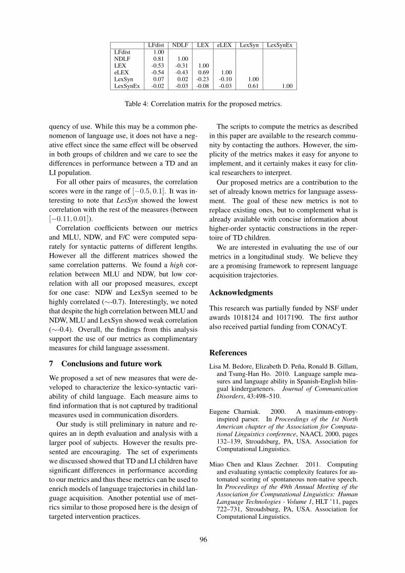
LFdist NDLF LEX eLEX LexSyn LexSynExLFdist 1.00NDLF 0.81 1.00LEX -0.53 -0.31 1.00eLEX -0.54 -0.43 0.69 1.00LexSyn 0.07 0.02 -0.23 -0.10 1.00LexSynEx -0.02 -0.03 -0.08 -0.03 0.61 1.00
Table 4: Correlation matrix for the proposed metrics.
quency of use. While this may be a common phe-nomenon of language use, it does not have a neg-ative effect since the same effect will be observedin both groups of children and we care to see thedifferences in performance between a TD and anLI population.
For all other pairs of measures, the correlationscores were in the range of [−0.5, 0.1]. It was in-teresting to note that LexSyn showed the lowestcorrelation with the rest of the measures (between[−0.11, 0.01]).
Correlation coefficients between our metricsand MLU, NDW, and F/C were computed sepa-rately for syntactic patterns of different lengths.However all the different matrices showed thesame correlation patterns. We found a high cor-relation between MLU and NDW, but low cor-relation with all our proposed measures, exceptfor one case: NDW and LexSyn seemed to behighly correlated (∼-0.7). Interestingly, we notedthat despite the high correlation between MLU andNDW, MLU and LexSyn showed weak correlation(∼-0.4). Overall, the findings from this analysissupport the use of our metrics as complimentarymeasures for child language assessment.
7 Conclusions and future work
We proposed a set of new measures that were de-veloped to characterize the lexico-syntactic vari-ability of child language. Each measure aims tofind information that is not captured by traditionalmeasures used in communication disorders.
Our study is still preliminary in nature and re-quires an in depth evaluation and analysis with alarger pool of subjects. However the results pre-sented are encouraging. The set of experimentswe discussed showed that TD and LI children havesignificant differences in performance accordingto our metrics and thus these metrics can be used toenrich models of language trajectories in child lan-guage acquisition. Another potential use of met-rics similar to those proposed here is the design oftargeted intervention practices.
The scripts to compute the metrics as describedin this paper are available to the research commu-nity by contacting the authors. However, the sim-plicity of the metrics makes it easy for anyone toimplement, and it certainly makes it easy for clin-ical researchers to interpret.
Our proposed metrics are a contribution to theset of already known metrics for language assess-ment. The goal of these new metrics is not toreplace existing ones, but to complement what isalready available with concise information abouthigher-order syntactic constructions in the reper-toire of TD children.
We are interested in evaluating the use of ourmetrics in a longitudinal study. We believe theyare a promising framework to represent languageacquisition trajectories.
Acknowledgments
This research was partially funded by NSF underawards 1018124 and 1017190. The first authoralso received partial funding from CONACyT.
ReferencesLisa M. Bedore, Elizabeth D. Pena, Ronald B. Gillam,
and Tsung-Han Ho. 2010. Language sample mea-sures and language ability in Spanish-English bilin-gual kindergarteners. Journal of CommunicationDisorders, 43:498–510.
Eugene Charniak. 2000. A maximum-entropy-inspired parser. In Proceedings of the 1st NorthAmerican chapter of the Association for Computa-tional Linguistics conference, NAACL 2000, pages132–139, Stroudsburg, PA, USA. Association forComputational Linguistics.
Miao Chen and Klaus Zechner. 2011. Computingand evaluating syntactic complexity features for au-tomated scoring of spontaneous non-native speech.In Proceedings of the 49th Annual Meeting of theAssociation for Computational Linguistics: HumanLanguage Technologies - Volume 1, HLT ’11, pages722–731, Stroudsburg, PA, USA. Association forComputational Linguistics.
96
Keyur Gabani, Melissa Sherman, Thamar Solorio,Yang Liu, Lisa M. Bedore, and Elizabeth D. Pena.2009. A corpus-based approach for the predictionof language impairment in monolingual English andSpanish-English bilingual children. In Proceedingsof Human Language Technologies: The 2009 An-nual Conference of the North American Chapterof the Association for Computational Linguistics,NAACL ’09, pages 46–55, Stroudsburg, PA, USA.Association for Computational Linguistics.
V. Gutierrez-Clellen, G. Simon-Cereijido, andM. Sweet. 2012. Predictors of second languageacquisition in Latino children with specific languageimpairment. American Journal of Speech LanguagePathology, 21(1):64–77.
Khairun-nisa Hassanali, Yang Liu, and ThamarSolorio. 2012a. Coherence in child language narra-tives: A case study of annotation and automatic pre-diction of coherence. In Proceedings of 3rd Work-shop on Child, Computer and Interaction (WOCCI2012).
Khairun-nisa Hassanali, Yang Liu, and ThamarSolorio. 2012b. Evaluating NLP features for auto-matic prediction of language impairment using childspeech transcripts. In Interspeech.
Tom Kwiatkowski, Sharon Goldwater, Luke Zettel-moyer, and Mark Steedman. 2012. A probabilis-tic model of syntactic and semantic acquisition fromchild-directed utterances and their meanings. InProceedings of the 13th Conference of the EuropeanChapter of the Association for Computational Lin-guistics, pages 234–244, Avignon, France. Associa-tion for Computational Linguistics.
Xiaofei Lu. 2012. The relationship of lexical richnessto the quality of ESL learners’ oral narratives. TheModern Language Journal, 96(2):190–208.
Mercer Mayer. 1967. A boy, a dog, and a frog. DialPress.
Mercer Mayer. 1969. Frog, where are you? DialPress.
Jon F. Miller, John Heilmann, Ann Nockerts, AquilesIglesias, Leah Fabiano, and David J. Francis. 2006.Oral language and reading in bilingual children.Learning Disabilities Research and Practice, 21:30–43.
Elizabeth D. Pena, Lisa M. Bedore, Ronald B. Gillam,and Thomas Bohman. 2003. Diagnostic markersof language impairment in bilingual children. Grantawarded by the NIDCH, NIH.
Emily T. Prud’hommeaux, Brian Roark, Lois M.Black, and Jan van Santen. 2011. Classification ofatypical language in autism. In Proceedings of the2nd Workshop on Cognitive Modeling and Compu-tational Linguistics, pages 88–96, Portland, Oregon,USA, June. Association for Computational Linguis-tics.
Brian Roark, Margaret Mitchell, and Kristy Holling-shead. 2007. Syntactic complexity measures fordetecting mild cognitive impairment. In Biologi-cal, translational, and clinical language processing,pages 1–8, Prague, Czech Republic, June. Associa-tion for Computational Linguistics.
Brian Roark, Margaret Mitchell, John-Paul Hosom,Kristy Hollingshead, and Jeffrey Kaye. 2011. Spo-ken language derived measures for detecting mildcognitive impairment. IEEE Transcations on Au-dio, Speech, and Language Processing, 19(7):2081–2090, September.
Raul Rojas and Aquiles Iglesias. 2012. The languagegrowth of Spanish-speaking English language learn-ers. Child Development.
Kenji Sagae, Alon Lavie, and Brian MacWhinney.2005. Automatic measurement of syntactic devel-opment in child language. In Proceedings of the43rd Annual Meeting of the Association for Com-putational Linguistics, ACL ’05, pages 197–204,Stroudsburg, PA, USA. Association for Computa-tional Linguistics.
Sam Sahakian and Benjamin Snyder. 2012. Automat-ically learning measures of child language develop-ment. In ACL, pages 95–99. The Association forComputational Linguistics.
Thamar Solorio, Melissa Sherman, Y. Liu, LisaBedore, Elizabeth Pena, and A. Iglesias. 2011. An-alyzing language samples of Spanish-English bilin-gual children for the automated prediction of lan-guage dominance. Natural Language Engineering,pages 367–395.
Charles Yang. 2011. A statistical test for grammar.In Proceedings of the 2nd Workshop on CognitiveModeling and Computational Linguistics, pages 30–38, Portland, Oregon, USA, June. Association forComputational Linguistics.
Su-Youn Yoon and Suma Bhat. 2012. Assessment ofESL learners’ syntactic competence based on sim-ilarity measures. In EMNLP-CoNLL, pages 600–608. Association for Computational Linguistics.
97
Proceedings of the 2013 Workshop on Biomedical Natural Language Processing (BioNLP 2013), pages 98–101,Sofia, Bulgaria, August 4-9 2013. c©2013 Association for Computational Linguistics
Adapting a parser to clinical text by simple pre-processing rules
Maria SkeppstedtDept. of Computer and Systems Sciences (DSV)
Stockholm University, Forum 100, 164 40 Kista, [email protected]
AbstractSentence types typical to Swedish clini-cal text were extracted by comparing sen-tence part-of-speech tag sequences in clin-ical and in standard Swedish text. Parsingsby a syntactic dependency parser, trainedon standard Swedish, were manually ana-lysed for the 33 sentence types most typ-ical to clinical text. This analysis re-sulted in the identification of eight errortypes, and for two of these error types, pre-processing rules were constructed to im-prove the performance of the parser. Forall but one of the ten sentence types af-fected by these two rules, the parsing wasimproved by pre-processing.
1 Introduction
Input speed is often prioritised over completenessand grammatical correctness in health record nar-ratives. This has the effect that lower results areachieved when parsers trained on standard text areapplied on clinical text (Hassel et al., 2011).
Syntactic annotations to use for training a parseron clinical text are, however, expensive (Albrightet al., 2013) and treebanking large clinical corporais therefore not always an option for smaller lan-guages (Haverinen et al., 2009). There are studieson adaptation of standard parsers to the biomedicaldomain, focusing on overcoming difficulties dueto different vocabulary use (Candito et al., 2011).How to overcome difficulties due to syntactic dif-ferences between standard and clinical languageis, however, less studied. The aim of this studywas therefore to explore syntactic differences be-tween clinical language and standard language andto analyse errors made by the parser on sentencetypes typical to the clinical domain. To exemplifyhow this knowledge can be used, two simple pre-processing rules for improving parser performanceon these typical sentences were developed.
2 Method
To find sentence types typical to the clinical do-main, a comparison to standard text was con-ducted. The used clinical corpus was: free-textentries from assessment sections, thus mostly con-taining diagnostic reasoning, that were randomlyselected from the Stockholm EPR corpus1 (Dalia-nis et al., 2009); and the used standard corpuswas: Lakartidningen (Kokkinakis, 2012), a jour-nal from the Swedish Medical Association.
The comparison was carried out on part-of-speech sequences on a sentence level. The part-of-speech tagger Granska (Carlberger and Kann,1999), having an accuracy of 92% on clinical text(Hassel et al., 2011), was applied on both cor-pora, and the proportion of each sentence tag se-quence was calculated. ’Sentence tag sequence’refers here to the parts-of-speech corresponding toeach token in the sentence, combined to one unit,e.g. ’dt nn vb nn mad’ for the sentence ’The pa-tient has headache.’. Pronouns, nouns and propernames were collapsed into one class, as they oftenplay the same role in the sentence, and as termsspecific to the clinical domain are tagged inconsis-tently as either nouns or proper names (Hassel etal., 2011). As sentences from Lakartidningen notending with a full stop or a question mark are lesslikely to be full sentences, they were not included,in order to obtain a more contrasting corpus.
A 95% confidence interval for the proportion ofeach sentence combination was computed usingthe Wilson score interval, and the difference be-tween the minimum frequency in the clinical cor-pus and the maximum frequency in the standardlanguage corpus was calculated. Thereby, statis-tics for the minimum difference between the twodomains was achieved.
1This research has been approved by the Regional EthicalReview Board in Stockholm (Etikprovningsnamnden i Stock-holm), permission number 2012/834-31/5.
98
A total of 458 436 sentence types were foundin the clinical corpus. Of these, there were 1 736types significantly more frequent in the clinicalcorpus than in the standard corpus, not havingoverlapping confidence interval for the propor-tions. 33 sentence types, to which 10% of the sen-tences in the corpus belonged, had more than 0.1percentage points difference between minimumfrequency in the clinical corpus and maximum fre-quency in the standard language corpus. For eachof these 33 sentence types, 30 sentences were ran-domly extracted and the dependency parser Malt-Parser (Nivre et al., 2009), pre-trained on Tal-banken (Nivre et al., 2006) using the algorithmstacklazy (Nivre et al., 2009), was applied to thesepart-of-speech tagged sentences. Error categorieswere manually identified, using MaltEval (Nilssonand Nivre, 2008) for visualisation.
Given the identified error categories, two pre-processing rules were constructed. These werethen evaluated by applying the same pre-trainedparser model on pre-processed sentences as onoriginal sentences. A manual analysis was per-formed on a subset of the sentences that were dif-ferently parsed after pre-processing.
3 Results
Although only one sentence type was a full sen-tence (nn vb pp nn mad), most sentences werecorrectly parsed. Omitted words could be inferredfrom context, and therefore also the intended syn-tax. Eight error types, to which most errors be-longed, were identified: 1) Abbreviated wordsending with a full stop interpreted as the last wordin a sentence, resulting in an incorrect sentencesplitting. 2) Abbreviations incorrectly labelled asnouns by Granska, resulting in sentences exclu-sively containing nouns. 3) Adjectives not recog-nised as such (often because they were abbrevi-ated), resulting in AT relations being labelled asDT relations. 4) A general adverbial relation in-correctly assigned an adverb of place or time rela-tion or vice versa. 5) The first word in compoundexpressions parsed as a determiner to the second.6) nn pp nn pp nn mad sentences for which apreposition had been incorrectly attributed. 7) Thesentence type nn jj (noun adjective), for whichmost evaluated sentences were incorrectly parsed.8) An omitted initial subject, resulting in the ob-ject incorrectly being parsed as the subject of thesentence.
Pre-processing rules were constructed for errortypes 7) and 8). As a verb in the middle of nnjj-sentences (in most cases copula) was left out,the first pre-processing rule added copula in themiddle of these sentences. The second rule addedthe pronoun I as the first word in sentences startingwith a verb, as this was the most frequently leftout subject, along with the slightly less frequentomission, patient. The rules were not applied onsentences ending with a question mark.
10 (out of 33) sentence types were affected bythe two rules. The proportion of those receiving adifferent parsing after pre-processing is shown inthe column Changed in Table 1. A subset of thesesentences, for which the parsing was changed, wasmanually classified as either incorrect (= contain-ing at least one parsing or labelling error) or com-pletely correct.
For sentences classified as incorrect, a moregranular comparison between the original and themodified parsing was carried out. For these sen-tences, the difference in average unlabelled (UAS)and labelled (LAS) attachment score between thepre-processed and the original parsing was com-puted. A positive value indicates that although thepre-processing resulted in some incorrectly parsedsentences, these sentences were improved by pre-processing. The sentence types vb pp nn nn madand vb pp nn pp nn mad were thus slightly im-proved by the pre-processing, although they had alow proportion of correctly parsed sentences.
A negative value for attachment score differ-ence, on the other hand, indicates that parsing forthe incorrectly parsed sentences was impaired bypre-processing. As these figures only apply to sen-tences incorrectly parsed after pre-processing, thismeans that although e.g. the type vb ab nn madhas negative UAS and LAS difference, this onlyapplies to the 3 sentences that were incorrectlyparsed by the pre-processed version.
With one important exception, sentences modi-fied by pre-processing, were either a) given a com-pletely correct parsing and labelling in between64% and 100% of the cases, or were b) slightlyimproved by pre-processing. A reasonable sim-plification in this case is that there can only beone correct parsing of a sentence, as althoughthere might be occurrences of syntactically am-biguous sentences, it is unlikely that their inter-pretation is not given by the context in the closeddomain of language used for diagnostic reasoning.
99
Given this simplification, this means that a sen-tence was transformed from an incorrectly parsedsentence to a correctly parsed sentence in 64% ormore of the cases, when pre-processing was ap-plied. The difference in attachment score showsthat the parsing is not drastically degraded for therest of the sentences, although it mostly changedto a worse parsing. The overall effect of apply-ing pre-processing is therefore positive. Sentencesof the type vb nn pp nn mad is the important ex-ception to this positive effect, important as 54% ofthe sentences belonging to this type received a dif-ferent parsing after pre-processing and as 0.39%of the sentences in the corpus belong to this type.Only 61% of the pre-processed sentences of thistype had a correct unlabelled parsing and only32% had a correct labelled parsing. Many of thesesentences were similar to Writes a prescription ofTrombyl, for which of Trombyl incorrectly is giventhe word write as the head after pre-processing.
Almost all of the sentences of the type nn jj madwere correctly parsed when a copula was insertedbetween the noun and the adjective. Of the othertypes of sentences that improved, many improvedby an incorrectly labelled subject relation beingchanged to an object relation. There were, how-ever, also improvements because some adverbs ofplace and time were correctly labelled after thepre-processing rules had been applied.
4 Discussion
Even if quantitative data is given in Table 1, thecore of this study has been to use a qualitative ap-proach: searching for different categories of errorsrather than determining accuracy figures, and in-vestigating whether pre-processing has a positiveeffect, rather than determining the final accuracy.
The next step is to apply the findings of thisstudy for developing a small treebank of clinicaltext. A possible method for facilitating syntacticannotation is to present pre-annotated data to theannotator (Brants and Plaehn, 2000) for correctionor for selection among several alternatives. As theoverall effect of applying pre-processing were im-proved parsings, the pre-annotation could be car-ried out by applying a model trained on standardlanguage and improve it with the pre-processingrules investigated here. The other identified errortypes also give suggestions of how to improve theparser, improvements that should be attempted be-fore using a parser trained on standard language
for pre-annotation. Error types 1), 2) and partly3) were due to abbreviations negatively affect-ing part-of-speech tagging and sentence splitting.Therefore, abbreviation expansion would be a pos-sible way of improving the parser. That availablemedical vocabularies also could be useful is shownby error type 5), which was due to the parser fail-ing to recognise compound expressions.
Of the sentences in the corpus, only 10%belonged to the analysed sentence types, andeven fewer were affected by the evaluated pre-processing rules. It is, however, likely that the twodeveloped pre-processing rules have effects on allsentence types lacking a verb or starting with averb, thus effecting more sentence type than thoseincluded in this study. This is worth studying,as is also syntactic differences for shorter part-of-speech sequences than sentence level sequences.
Another possible method for domain adaptationwould be to adapt the training data to construct amodel more suitable for parsing clinical text. In-stead of applying pre-processing, sentences in thetraining data could be modified to more closely re-semble sentences in clinical text, e.g. by removingwords in the treebank corpus to achieve the incom-plete sentences typical to clinical text. Differencesin vocabulary has not been included in this study,but methods from previous studies for bridgingdifferences in vocabulary between the general andmedical domain could also be applied for improv-ing parser performance.
For supplementing a treebank to also includesentences typical to clinical text, some of themethods investigated here for extracting such sen-tence types, could be employed
5 Conclusion
Sentence types typical to clinical text were ex-tracted, and eight categories of error types wereidentified. For two of these error types, pre-processing rules were devised and evaluated.For four additional error types, techniques fortext-normalisation were suggested. As the pre-processing rules had an overall positive effect onthe parser performance, it was suggested that amodel for syntactic pre-annotation of clinical textshould employ the evaluated text pre-processing.
Acknowledgements
Many thanks to Joakim Nivre and to the four re-viewers for their many valuable comments.
100
Sentence # % # % Correct # Incorrect pp UAS(LAS)type In test Changed Manually unlabelled unlabelled difference am-
classified (labelled) (labelled) ong incorrecta) vb nn mad 1181 30% 40 100 (100)% 0 (0)
vb jj nn mad 317 13% 32 100 (94) % 0 (2)nn jj mad 316 100% 200 94 (94) % 12 (12)vb ab nn mad 256 33% 31 90 (90) % 3 (3) -25 (-25) ppvb pp nn mad 674 5% 27 100 (85) % 0 (4) (-19) ppvb ab pp nn mad 222 21% 30 100 (70) % 0 (9) (+7) ppvb pp jj nn mad 207 7% 14 100 (64) % 0 (5) (-16) pp
b) vb pp nn nn mad 197 5% 9 22 (11) % 7 (8) 0 (+10) ppvb pp nn pp nn mad 232 5% 12 75 (4) % 3 (12) 0 (+2) pp
c) vb nn pp nn mad 813 54% 28 61 (32) % 11 (19) -20 (-15) pp
Table 1: In test: Number of sentences in test set of this type. Changed: Proportion of sentences thatreceived a different parsing after pre-processing had been applied. Manually classified: Number of man-ually classified sentences. Correct: Proportion of sentences that were correctly parsed (and labelled)after pre-processing had been applied. # Incorrect: Number of incorrectly parsed (and labelled) sen-tences after pre-processing. UAS (LAS) difference: For these incorrect sentences: The difference in UAS,unlabelled attachment score, (and LAS, labelled attachment score) before and after pre-processing. (Forsentence types with more than 90% correct sentences, this difference was not calculated.)
ReferencesDaniel Albright, Arrick Lanfranchi, Anwen Fredrik-
sen, William F Styler, 4th, Colin Warner, Jena DHwang, Jinho D Choi, Dmitriy Dligach, Rod-ney D Nielsen, James Martin, Wayne Ward, MarthaPalmer, and Guergana K Savova. 2013. Towardscomprehensive syntactic and semantic annotationsof the clinical narrative. J Am Med Inform Assoc,Jan.
Thorsten Brants and Oliver Plaehn. 2000. Interactivecorpus annotation. In LREC. European LanguageResources Association.
Marie Candito, Enrique H. Anguiano, and Djame Sed-dah. 2011. A Word Clustering Approach to DomainAdaptation: Effective Parsing of Biomedical Texts.In Proceedings of the 12th International Conferenceon Parsing Technologies, pages 37–42, Dublin, Ire-land, October. Association for Computational Lin-guistics.
Johan Carlberger and Viggo Kann. 1999. Implement-ing an efficient part-of-speech tagger. Software–Practice and Experience, 29:815–832.
Hercules Dalianis, Martin Hassel, and SumithraVelupillai. 2009. The Stockholm EPR Corpus -Characteristics and Some Initial Findings. In Pro-ceedings of ISHIMR 2009, Evaluation and imple-mentation of e-health and health information initia-tives: international perspectives. 14th InternationalSymposium for Health Information Management Re-search, Kalmar, Sweden, pages 243–249.
Martin Hassel, Aron Henriksson, and SumithraVelupillai. 2011. Something Old, Something New
- Applying a Pre-trained Parsing Model to Clini-cal Swedish. In Proceedings of NODALIDA’11 -18th Nordic Conference on Computational Linguis-tics, Riga, Latvia, May 11-13.
Katri Haverinen, Filip Ginter, Veronika Laippala, andTapio Salakoski. 2009. Parsing Clinical Finnish:Experiments with Rule-Based and Statistical De-pendency Parsers. In Kristiina Jokinen and Eck-hard Bick, editors, Proceedings of NODALIDA’09,Odense, Denmark, pages 65–72.
Dimitrios Kokkinakis. 2012. The journal of theSwedish medical association - a corpus resource forbiomedical text mining in Swedish. In The ThirdWorkshop on Building and Evaluating Resources forBiomedical Text Mining (BioTxtM), an LREC Work-shop. Turkey.
Jens Nilsson and Joakim Nivre. 2008. Malteval:An evaluation and visualization tool for dependencyparsing. In Proceedings of the Sixth InternationalLanguage Resources and Evaluation. LREC, pages161–166.
Joakim Nivre, Jens Nilsson, and Johan Hall. 2006. Tal-banken05: A Swedish treebank with phrase struc-ture and dependency annotation. In Proceedings ofthe fifth international conference on Language Re-sources and Evaluation (LREC 2006), pages 24–26.
Joakim Nivre, Marco Kuhlmann, and Johan Hall.2009. An improved oracle for dependency parsingwith online reordering. In Proceedings of the 11thInternational Conference on Parsing Technologies,IWPT ’09, pages 73–76, Stroudsburg, PA, USA. As-sociation for Computational Linguistics.
101
Proceedings of the 2013 Workshop on Biomedical Natural Language Processing (BioNLP 2013), pages 102–110,Sofia, Bulgaria, August 4-9 2013. c©2013 Association for Computational Linguistics
Using the argumentative structure of scientific literature to improveinformation access
Antonio Jimeno YepesNational ICT Australia
Victoria Research LaboratoryMelbourne, Australia
James G. MorkNational Library of Medicine
8600 Rockville PikeBethesda, 20894, MD, [email protected]
Alan R. AronsonNational Library of Medicine
8600 Rockville PikeBethesda, 20894, MD, [email protected]
Abstract
MEDLINE/PubMed contains structuredabstracts that can provide argumentativelabels. Selection of abstract sentencesbased on the argumentative label hasshown to improve the performance of in-formation retrieval tasks. These abstractsmake up less than one quarter of all theabstracts in MEDLINE/PubMed, so it isworthwhile to learn how to automaticallylabel the non-structured ones.
We have compared several machine learn-ing algorithms trained on structured ab-stracts to identify argumentative labels.We have performed an intrinsic evalua-tion on predicting argumentative labels fornon-structured abstracts and an extrinsicevaluation to predict argumentative labelson abstracts relevant to Gene ReferenceInto Function (GeneRIF) indexing.
Intrinsic evaluation shows that argumen-tative labels can be assigned effectivelyto structured abstracts. Algorithms thatmodel the argumentative structure seemto perform better than other algorithms.Extrinsic results show that assigning ar-gumentative labels to non-structured ab-stracts improves the performance onGeneRIF indexing. On the other hand, thealgorithms that model the argumentativestructure of the abstracts obtain lower per-formance in the extrinsic evaluation.
1 Introduction
MEDLINE R©/PubMed R© is the largest repositoryof biomedical abstracts. The large quantity ofunstructured information available from MED-LINE/PubMed prevents finding information effi-ciently. Reducing the information that users needto process could improve information access and
support database curation. It has been suggestedthat identifying the argumentative label of the ab-stract sentences could provide better informationthrough information retrieval (Ruch et al., 2003;Jonnalagadda et al., 2012) and/or information ex-traction (Mizuta et al., 2006).
Some journals indexed in MEDLINE/PubMedalready provide the abstracts in a structured for-mat (Ripple et al., 2012). A structured abstract1 isan abstract with distinct labeled sections (e.g., In-troduction, Background, or Results). In the MED-LINE/PubMed data, these labels usually appear inall uppercase letters and are followed by a colon(e.g., MATERIALS AND METHODS:). Structuredabstracts are becoming an increasingly larger seg-ment of the MEDLINE/PubMed database with al-most a quarter of all abstracts added to the MED-LINE/PubMed database each year being struc-tured abstracts. A recent PubMed query (April 22,2013) shows 1,050,748 citations from 2012, and249,196 (23.72%)2 of these are considered struc-tured abstracts.
On August 16, 2010, PubMed began display-ing structured abstracts formatted to highlight thevarious sections within the structured abstracts tohelp readers identify areas of interest3. The XMLformatted abstract from MEDLINE/PubMed sep-arates each label in the structured abstract and in-cludes a mapping to one of five U.S. National Li-brary of Medicine (NLM) assigned categories asshown in the example below:
<AbstractText Label=”MATERIALS ANDMETHODS” NlmCategory=”METHODS”>
The five NLM categories that all labelsare mapped to are OBJECTIVE, CONCLU-SIONS, RESULTS, METHODS, and BACK-GROUND (Ripple et al., 2011). If a label is new
1http://www.nlm.nih.gov/bsd/policy/structured abstracts.html2hasstructuredabstract AND 2012[pdat]3http://www.nlm.nih.gov/pubs/techbull/ja10/ja10 structured abstracts.html
102
or not in the list of reviewed structured abstract la-bels, it will receive a category of UNASSIGNED.There are multiple criteria for deciding what ab-stracts are considered structured abstracts or not.One simple definition would be that an abstractcontains one or more author defined labels. Amore rigid criterion which is followed by NLM4
is that an abstract must contain three or moreunique valid labels (previously identified and cat-egorized), and one of the labels must be an endingtype label (e.g., CONCLUSIONS). The five NLMcategories are normally manually reviewed and as-signed once a year to as many new labels as pos-sible. Currently, NLM has identified 1,949 (Au-gust 31, 2012) unique labels and categorized theminto one of the five categories. These 1,949 labelsmake up approximately 98% of all labels and la-bel variations found in the structured abstracts inMEDLINE/PubMed3. An example of structuredabstract is presented in Table 1.
Several studies have shown that the labels of thestructured abstracts can be reassigned effectivelybased on a Conditional Random Field (CRF) mod-els (Hirohata et al., 2008). On the other hand, itis unclear if these models are as effective on non-structured abstracts (Agarwal and Yu, 2009).
In this paper, we compare several learning al-gorithms trained on structured abstract data to as-sign argumentative labels to non-structured ab-stracts. We performed comparison tests of thetrained models both intrinsically on a held out setof the structured abstracts and extrinsically on aset of non-structured abstracts.
The intrinsic evaluation is performed on a dataset of held out structured abstracts that have hadtheir label identification removed to model non-structured abstracts. Argumentative labels are as-signed to the sentences based on the trained mod-els and used to identify label categorization.
The extrinsic evaluation is performed on a dataset of non-structured abstracts on the task of iden-tifying GeneRIF (Gene Into Function) sentences.Argumentative labels are assigned to the sentencesbased on the trained models and used to performthe selection of relevant GeneRIF sentences.
Intrinsic evaluation shows that argumentativelabels can be assigned effectively to structured ab-stracts. Algorithms that model the argumentativestructure, like Conditional Random Field (CRF),seem to perform better than other algorithms. Re-
4http://structuredabstracts.nlm.nih.gov/Implementation.shtml
sults show that using the argumentative labels as-signed by the learning algorithms improves theperformance in GeneRIF sentence selection. Onthe other hand, models like CRF, which bettermodel the argumentative structure of the struc-tured abstracts, tend to perform below other learn-ing algorithms on the extrinsic evaluation. Thisshows that non-structured abstracts do not have thesame layout compared to structured ones.
2 Related work
As presented in the introduction, one of the ob-jectives of our work is to assign structured ab-stract labels to abstracts without these labels. Theidea is to help in the curation process of exist-ing databases and to improve the efficiency ofinformation access. Previous work on MED-LINE/PubMed abstracts has focused on learningto identify these labels mainly in the RandomizedControl Trials (RCT) domain. (McKnight andSrinivasan, 2003) used a Support Vector Machine(SVM) and a linear classifier and tried to pre-dict the labels of MEDLINE structured abstracts.Their work finds that it is possible to learn a modelto label the abstract with modest results. Furtherstudies have been conducted by (Ruch et al., 2003;Tbahriti et al., 2005; Ruch et al., 2007) to usethe argumentative model of the abstracts. Theyhave used this to improve retrieval and indexing ofMEDLINE citations, respectively. In their work,they have used a multi-class Naıve Bayes classi-fier.
(Hirohata et al., 2008) have shown that the la-bels in structured abstracts follow a certain argu-mentative structure. Using the current set of labelsused at the NLM, a typical argumentative struc-ture consists of OBJECTIVE, METHODS, RE-SULTS and CONCLUSION. This notion is some-what already explored by (McKnight and Srini-vasan, 2003) by using the position of the sentence.
More advanced approaches have been used thattrain a model that considers the sequence of labelsin the structured abstracts. (Lin et al., 2006) used agenerative model, comparing them to discrimina-tive ones. More recent work has been dealing withConditional Random Fields (Hirohata et al., 2008)with good performance.
(Agarwal and Yu, 2009) used similar ap-proaches and evaluated the labeling of full textarticles with the trained model on structured ab-stracts. Their evaluation included as well a set of
103
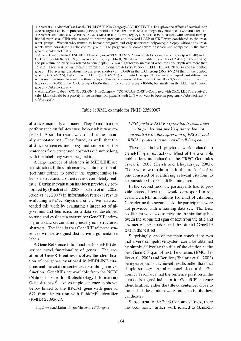
<Abstract> <AbstractText Label=”PURPOSE” NlmCategory=”OBJECTIVE”>To explore the effects of cervical loopelectrosurgical excision procedure (LEEP) or cold knife conization (CKC) on pregnancy outcomes.</AbstractText><AbstractText Label=”MATERIALS AND METHODS” NlmCategory=”METHODS”>Patients with cervical intraep-ithelial neoplasia (CIN) who wanted to become pregnant and received LEEP or CKC were considered as the treat-ment groups. Women who wanted to become pregnant and only underwent colposcopic biopsy without any treat-ments were considered as the control group. The pregnancy outcomes were observed and compared in the threegroups.</AbstractText><AbstractText Label=”RESULTS” NlmCategory=”RESULTS”>Premature delivery rate was higher (p = 0.048) in theCKC group (14/36, 38.88%) than in control group (14/68, 20.5%) with a odds ratio (OR) of 2.455 (1.007 - 5.985);and premature delivery was related to cone depth, OR was significantly increased when the cone depth was more than15 mm. There was no significant difference in premature delivery between LEEP (10 / 48, 20.83%) and the controlgroups. The average gestational weeks were shorter (p = 0.049) in the CKC group (36.9 +/- 2.4) than in the controlgroup (37.8 +/- 2.6), but similar in LEEP (38.1 +/- 2.4) and control groups. There were no significant differencesin cesarean sections between the three groups. The ratio of neonatal birth weight less than 2,500 g was significantlyhigher (p = 0.005) in the CKC group (15/36) than in the control group (10/68), but similar in the LEEP and controlgroups.</AbstractText><AbstractText Label=”CONCLUSION” NlmCategory=”CONCLUSIONS”>Compared with CKC, LEEP is relativelysafe. LEEP should be a priority in the treatment of patients with CIN who want to become pregnant.</AbstractText></Abstract>
Table 1: XML example for PMID 23590007
abstracts manually annotated. They found that theperformance on full-text was below what was ex-pected. A similar result was found in the manu-ally annotated set. They found, as well, that theabstract sentences are noisy and sometimes thesentences from structured abstracts did not belongwith the label they were assigned to.
A large number of abstracts in MEDLINE arenot structured; thus intrinsic evaluation of the al-gorithms trained to predict the argumentative la-bels on structured abstracts is not completely real-istic. Extrinsic evaluation has been previously per-formed by (Ruch et al., 2003; Tbahriti et al., 2005;Ruch et al., 2007) in information retrieval resultsevaluating a Naıve Bayes classifier. We have ex-tended this work by evaluating a larger set of al-gorithms and heuristics on a data set developedto tune and evaluate a system for GeneRIF index-ing on a data set containing mostly non-structuredabstracts. The idea is that GeneRIF relevant sen-tences will be assigned distinctive argumentativelabels.
A Gene Reference Into Function (GeneRIF) de-scribes novel functionality of genes. The cre-ation of GeneRIF entries involves the identifica-tion of the genes mentioned in MEDLINE cita-tions and the citation sentences describing a novelfunction. GeneRIFs are available from the NCBI(National Center for Biotechnology Information)Gene database5. An example sentence is shownbelow linked to the BRCA1 gene with gene id672 from the citation with PubMed R© identifier(PMID) 22093627:
5http://www.ncbi.nlm.nih.gov/sites/entrez?db=gene
FISH-positive EGFR expression is associatedwith gender and smoking status, but not
correlated with the expression of ERCC1 andBRCA1 proteins in non-small cell lung cancer.
There is limited previous work related toGeneRIF span extraction. Most of the availablepublications are related to the TREC GenomicsTrack in 2003 (Hersh and Bhupatiraju, 2003).There were two main tasks in this track, the firstone consisted of identifying relevant citations tobe considered for GeneRIF annotation.
In the second task, the participants had to pro-vide spans of text that would correspond to rel-evant GeneRIF annotations for a set of citations.Considering this second task, the participants werenot provided with a training data set. The Dicecoefficient was used to measure the similarity be-tween the submitted span of text from the title andabstract of the citation and the official GeneRIFtext in the test set.
Surprisingly, one of the main conclusions wasthat a very competitive system could be obtainedby simply delivering the title of the citation as thebest GeneRIF span of text. Few teams (EMC (Je-lier et al., 2003) and Berkley (Bhalotia et al., 2003)being exceptions), achieved results better than thatsimple strategy. Another conclusion of the Ge-nomics Track was that the sentence position in thecitation is a good indicator for GeneRIF sentenceidentification: either the title or sentences close tothe end of the citation were found to be the bestcandidates.
Subsequent to the 2003 Genomics Track, therehas been some further work related to GeneRIF
104
sentence selection. (Lu et al., 2006; Lu et al.,2007) sought to reproduce the results alreadyavailable from Entrez Gene (former name for theNCBI Gene database). In their approach, a setof features is identified from the sentences andused in the algorithm: Gene Ontology (GO) to-ken matches, cue words and sentence position inthe abstract. (Gobeill et al., 2008) combined argu-mentative features using discourse-analysis mod-els (LASt) and an automatic text categorizer toestimate the density of Gene Ontology categories(GOEx). The combination of these two featuresets produced results comparable to the best 2003Genomics Track system.
3 Methods
As in previous work, we approach the problemof learning to label sentences in abstracts us-ing machine learning methods on structured ab-stracts. We have compared a large range of ma-chine learning algorithms, including ConditionalRandom Field. The evaluation is performed in-trinsically on a held out set of structured abstractsand then evaluated extrinsically on a dataset devel-oped for the evaluation of algorithms for GeneRIFindexing.
3.1 Structured abstracts data set
This data set is used to train the machine learningalgorithms and to peform the intrinsic evaluationof structured abstracts. The abstracts have beencollected from PubMed using the query hasstruc-turedabstract, selecting the top 100k citations sat-ifying the query.
The abstract defined within the Abstract at-tribute is split into several AbstractText tags. EachAbstractText tag has the label Label that showsthe original label as provided by the journal whilethe NlmCategory represents the category as addedby the NLM.
From this set, 2/3 of the citations (66,666) areconsidered for training the machine learning algo-rithms while 1/3 of the citations (33,334) are re-served for testing. The abstract paragraphs havebeen split into sentences and the structured ab-stract label has been transferred to them. For in-stance, all the sentences in the INTRODUCTIONsection are labeled as INTRODUCTION.
An analysis of the abstracts has shown that thereare cases in which the article keywords were in-cluded as part of the abstract in a BACKGROUND
section. These were easily recognized by the orig-inal label KEYWORD. We have removed theseparagraphs since they are not typical sentencesin MEDLINE but a list of keywords. We findthat there are sections like OBJECTIVE where thenumber of sentences is very low, with less than 2sentences on average, while RESULTS is the sec-tion with the largest number of sentences on aver-age with over 4.5 sentences.
There are five candidate labels identified fromthe structured abstracts, presented in Table 2. Thedistribution of labels shows that some labels likeCONCLUSIONS, METHODS and RESULTS arevery frequent. CONCLUSIONS and METHODSare assigned to more than one paragraph since thenumber is bigger compared to the number of cita-tions in each set. This seems to happen when morethan one journal label in the same citation mapto METHODS or CONCLUSION, e.g. PMID:23538919.
Label Paragraphs SentencesBACKGROUND 53,348 132,890CONCLUSIONS 101,830 205,394METHODS 107,227 304,487OBJECTIVE 60,846 95,547RESULTS 95,824 436,653
Table 2: Structured abstracts data set statistics
We have compared the performance of sev-eral learning algorithms. Among other classi-fiers, we use Naıve Bayes and Linear Regression,which might be seen as a generative learner ver-sus discriminative (Jordan, 2002) learner. We haveused the implementation available from the Malletpackage (McCallum, 2002).
In addition to these two classifiers, we haveused AdaBoostM1 and SVM. SVM has beentrained using stochastic gradient descent (Zhang,2004), which is very efficient for linear ker-nels. Table 2 shows a large imbalance betweenthe labels, so we have used the modified HuberLoss (Zhang, 2004), which has already been usedin the context of MeSH indexing (Yeganova et al.,2011). Both algorithms were trained based on theone-versus-all approach. We have turned the algo-rithms into multi-class classifiers by selecting theprediction with the highest confidence by the clas-sifiers (Tsoumakas and Katakis, 2007). We haveused the implementation of these algorithms avail-
105
able from the MTI ML package6, previously usedin the task of MeSH indexing (Jimeno-Yepes et al.,2012).
The learning algorithms have been trained onthe text of the paragraph or sentences from thedata set presented above. The text is lowercasedand tokenized. In addition to the textual features,the position of the sentence or paragraph from thebeginning of the abstract is used as well.
As we have seen, argumentative structure of theabstract labels has been previously modeled usinga linear chain CRF (Lafferty et al., 2001). CRFis trained using the text features from sentences orparagraphs in conjunction of the abstract labels toperform the label assignment. In our experiments,we have used the implementation available fromthe Mallet package, using only an order 1 model.
3.2 GeneRIF data set
We have developed a data set to compare andevaluate GeneRIF indexing approaches (Jimeno-Yepes et al., 2013) as part of the Gene IndexingAssistant project at the NLM7. The current scopeof our work is limited to the human species. Thedevelopment is performed in two steps describedbelow. The first step consists of selecting cita-tions from journals typically associated with hu-man species. During the second step, we applyIndex Section rules for citation filtering plus ad-ditional rules to further focus the set of selectedcitations. Since there was no GeneRIF indexingbefore 2002, only articles from 2002 through 2011from the 2011 MEDLINE Baseline 8 (11/19/2010)were used to build the data set.
A subset of the filtered citations was collectedfor annotation. The annotations were performedby two annotators. Guidelines were prepared andtested on a small set by the two annotators and re-fined before annotating the entire set.
The data set has been annotated with GeneRIFcategories of the sentences. The categories are:Expression, Function, Isolation, Non-GeneRIF,Other, Reference, and Structure. We assigned theGeneRIF category to all the categories that didnot belong to Non-GeneRIF. The indexing task isthen to categorize the sentences into GeneRIF sen-tences and Non-GeneRIF ones. Based on their an-notation work on the data set, the F-measure for
6http://ii.nlm.nih.gov/MTI ML/index.shtml7http://www.lhncbc.nlm.nih.gov/project/automated-
indexing-research8http://mbr.nlm.nih.gov
the annotators is 0.81. We have used this annota-tion for the extrinsic evaluation of GeneRIF index-ing.
This data set has been further split into trainingand testing subsets. Table 3 shows the distributionbetween GeneRIF and Non-GeneRIF sentences.
Set Total GeneRIF Non-GeneRIFTraining 1987 829 (42%) 1158 (58%)Testing 999 433 (43%) 566 (57%)
Table 3: GeneRIF sentence distribution
In previous work, the indexing of GeneRIF sen-tences, on our data set, was performed based ona trained classifier on a set of features that per-formed well on the GeneRIF testing set (Jimeno-Yepes et al., 2013). Naıve Bayes was the learningalgorithm that performed the best compared to theother methods and has been selected in this workas the method to be used to combine the featuresof the argumentative labeling algorithms.
The set of features in the baseline experimentsinclude the position of the sentence from the be-ginning of the abstract, the position of the sentencecounting from the end of the abstract, the sen-tence text, the annotation of disease terms, basedon MetaMap (Aronson and Lang, 2010), and geneterms, based on a dictionary approach, and theGene Ontology term density (Gobeill et al., 2008).
4 Results
As mentioned before, we have performed the eval-uation of the algorithms intrinsically, given a setof structured abstracts, and extrinsically based ontheir performance on GeneRIF sentence indexing.
4.1 Intrinsic evaluation (structuredabstracts)
Tables 4 and 5 show the results of the intrinsicevaluation for paragraph and sentence experimentsrespectively. The algorithms are trained to labelthe paragraphs or sentences from the structuredabstracts. The precision (P), recall (R) and F1
(F) values are presented for each argumentative la-bel. The methods evaluated include Naıve Bayes(NB), Logistic Regression (LR), SVM based onmodified Huber Loss (Huber) and AdaBoostM1(ADA). These methods have been trained on thetext of either the sentence or the paragraph, andmight include their position feature, indicated withthe letter P (e.g. NB P for Naıve Bayes trained
106
Label NB NB P LR LR P ADA ADA P Huber HuberP CRFBACKGROUND P 0.6047 0.6853 0.6374 0.7369 0.6098 0.7308 0.5862 0.7166 0.7357
R 0.5672 0.7190 0.5868 0.7207 0.3676 0.7337 0.4984 0.6694 0.7093F 0.5854 0.7017 0.6110 0.7287 0.4587 0.7323 0.5387 0.6922 0.7223
CONCLUSIONS P 0.7532 0.8626 0.8365 0.9413 0.6975 0.8862 0.7578 0.9051 0.9769R 0.8606 0.9366 0.8675 0.9552 0.8246 0.9404 0.7987 0.9340 0.9784F 0.8033 0.8981 0.8517 0.9482 0.7557 0.9125 0.7777 0.9193 0.9776
METHODS P 0.9002 0.9278 0.9113 0.9396 0.8256 0.9041 0.8668 0.9116 0.9684R 0.9040 0.9126 0.9294 0.9493 0.8955 0.9250 0.9012 0.9237 0.9675F 0.9021 0.9201 0.9203 0.9444 0.8591 0.9144 0.8837 0.9176 0.9680
OBJECTIVE P 0.7294 0.7650 0.7167 0.7531 0.6763 0.7565 0.6788 0.7160 0.7608R 0.6453 0.7190 0.7255 0.7549 0.6937 0.7228 0.6733 0.7365 0.7759F 0.6848 0.7413 0.7210 0.7540 0.6849 0.7393 0.6761 0.7261 0.7683
RESULTS P 0.8841 0.9106 0.9086 0.9372 0.8554 0.9157 0.8560 0.9122 0.9692R 0.8414 0.8542 0.8857 0.9216 0.7842 0.8564 0.8447 0.8846 0.9758F 0.8622 0.8815 0.8970 0.9294 0.8182 0.8851 0.8503 0.8981 0.9725
Average P 0.7743 0.8303 0.8021 0.8616 0.7329 0.8387 0.7491 0.8323 0.8822R 0.7637 0.8283 0.7990 0.8604 0.7131 0.8357 0.7433 0.8296 0.8814F 0.7690 0.8293 0.8005 0.8610 0.7229 0.8372 0.7462 0.8310 0.8818
Table 4: Intrinsic evaluation of paragraph based labeling
Label NB NB P LR LR P ADA ADA P Huber HuberP CRFBACKGROUND P 0.4983 0.6313 0.5558 0.6862 0.4779 0.6417 0.5153 0.6495 0.6738
R 0.4980 0.6921 0.5084 0.7139 0.3207 0.6993 0.3372 0.6554 0.7104F 0.4981 0.6603 0.5311 0.6998 0.3838 0.6693 0.4076 0.6524 0.6916
CONCLUSIONS P 0.5876 0.7270 0.6794 0.8431 0.5672 0.7651 0.6153 0.7767 0.8977R 0.7103 0.8388 0.6788 0.8187 0.4998 0.6816 0.5163 0.7213 0.8671F 0.6431 0.7789 0.6791 0.8307 0.5314 0.7209 0.5615 0.7480 0.8821
METHODS P 0.7857 0.8206 0.8193 0.8549 0.7224 0.7793 0.7343 0.7894 0.8931R 0.8084 0.8366 0.8427 0.8696 0.7789 0.8152 0.7828 0.8250 0.8988F 0.7969 0.8285 0.8308 0.8622 0.7496 0.7968 0.7578 0.8068 0.8960
OBJECTIVE P 0.5522 0.6237 0.6032 0.6696 0.5497 0.6671 0.5525 0.6259 0.6258R 0.4894 0.5530 0.4995 0.5534 0.4082 0.4518 0.4479 0.5036 0.5779F 0.5189 0.5862 0.5465 0.6060 0.4685 0.5388 0.4947 0.5581 0.6009
RESULTS P 0.8294 0.8517 0.8071 0.8449 0.6903 0.7665 0.6957 0.7877 0.8892R 0.7517 0.7743 0.8429 0.8679 0.7998 0.8143 0.6957 0.8208 0.8995F 0.7886 0.8112 0.8246 0.8563 0.7410 0.7897 0.6957 0.8039 0.8943
Average P 0.6506 0.7309 0.6930 0.7797 0.6015 0.7239 0.6226 0.7258 0.7959R 0.6516 0.7390 0.6745 0.7647 0.5615 0.6924 0.5560 0.7052 0.7907F 0.6511 0.7349 0.6836 0.7721 0.5808 0.7078 0.5874 0.7154 0.7933
Table 5: Intrinsic evaluation of sentence based labeling
with the features from text and the position). Theresults include those based on CRF trained on thetext of either the sentence or the paragraph takinginto account the labeling sequence.
CRF has the best performance in both tables,with the differences being more dramatic on theparagraph results. These results are comparableto (Hirohata et al., 2008), even though we areworking with a different set of labels. Compar-ing the remaining learning algorithms, LR per-forms better than the other classifiers. Both Ad-aBoostM1 and SVM perform not as well as NBand LR; this could be due to the noise referredto by (Agarwal and Yu, 2009) that appears in thestructured abstract sentences. Considering eitherthe paragraph or the sentence text, the position in-formation helps improve their performance.
CONCLUSIONS, METHODS and RESULTSlabels have the best performance, which matchesthe most frequent labels in the dataset (see Ta-ble 2). BACKGROUND and OBJECTIVE haveworse performance compared to the other labels.These two labels have the largest imbalance com-pared to the other labels, which seems to nega-tively impact the classifiers performance.
The results based on the paragraphs outperformthe ones based on the sentences. Argumentativestructure of the paragraphs seems to be easier,probably due to the fact that individual sentenceshave been shown to be noisy (Agarwal and Yu,2009), and this could explain this behaviour.
107
4.2 Extrinsic evaluation (GeneRIFs)
Extrinsic evaluation is performed on the GeneRIFdata set presented in the Methods section. Theidea of the evaluation is to assign one of the ar-gumentative labels to the sentences, based on themodels trained on structured abstracts, and eval-uate the impact of this assignment in the selec-tion of GeneRIF sentences. From the set of ma-chine learning algorithms intrinsically evaluated,we have selected the LR models trained with andwithout position information (Pos) and the CRFmodel. The LR and CRF models are used to la-bel the GeneRIF training and testing data with theargumentative labels.
Table 6 shows the results of the extrinsic evalu-ation. Results obtained with the argumentative la-bel feature and with or without the set of featuresused in the baseline are compared to the baselinemodel, i.e. NB and the set of features presentedin the Methods section. In all the cases, precision(P), recall (R) and F1 using the argumentative fea-tures improve over the baseline.
The intrinsic evaluation was performed eitheron sentences or paragraphs. The sentence mod-els perform better than the paragraph based mod-els. We find as well that LR with sentence positionperforms slightly better than when combined withthe baseline features, with higher recall but lowerprecision. Contrary to the intrinsic results, LR per-forms better than CRF, even though both outper-form the baseline. This means that non-structuredsentences do not necessarily follow the same argu-mentative structure as the structured abstracts.
Label P R FBaseline 0.6210 0.6605 0.6405LR Par 0.7235 0.6767 0.6993LR Par + Base 0.7184 0.8014 0.7576LR Par Pos 0.5978 0.8891 0.7149LR Par Pos + Base 0.6883 0.8060 0.7426LR Sen 0.7039 0.7852 0.7424LR Sen + Base 0.7325 0.7968 0.7633LR Sen Pos 0.7014 0.9007 0.7887LR Sen Pos + Base 0.7222 0.8406 0.7769CRF Par 0.6682 0.6744 0.6713CRF Par + Base 0.7036 0.8060 0.7513CRF Sen 0.6536 0.8499 0.7390CRF Sen + Base 0.7134 0.7875 0.7486
Table 6: GeneRIF extrinsic evaluation
5 Discussion
Results show that it is possible to automaticallypredict the argumentative label of the structuredabstracts and to improve the performance forGeneRIF annotation. Intrinsic evaluation showsthat paragraph labeling is easier compared to sen-tence labeling, which might be partly due to thenoise in the sentences as identified by (Agarwaland Yu, 2009). The excellent performance forparagraph labeling was already shown by previouswork (Hirohata et al., 2008) while sentence label-ing issues for structured abstracts was previouslyintroduced by (Agarwal and Yu, 2009). In both in-trinsic tasks, adding the position of the paragraphor sentence improves the performance of the learn-ing algorithms.
Extrinsic evaluation shows that, compared tothe baseline features for GeneRIF annotation,adding argumentative labeling using the trainedmodels improves its performance, which is closeto the human performance reported in the Meth-ods section. On the other hand, we find that theCRF models show lower performance comparedto the LR models. From the LR models, the po-sition of the sentence or paragraph seems to havebetter performance.
In addition, the LR model trained on the sen-tences performs better compared to the modeltrained on the paragraphs. This might be partlydue to the fact that sentence based models seemto be better suited than the paragraph based onesas might have been expected. The fact that theCRF models performance is below the LR mod-els denotes that the structured abstracts seem tofollow a pattern that is different in the case ofnon-structured abstracts. Looking closer at theassigned labels, the LR models tend to assignmore CONCLUSIONS and RESULTS labels tothe GeneRIF sentences compared to the CRF ones.
6 Conclusions and Future Work
We have presented an evaluation of several learn-ing algorithms to label abstract text in MED-LINE/PubMed with argumentative labels, basedon MEDLINE/PubMed structured abstracts. Theresults show that this task can be achieved withhigh performance in the case of labeling the para-graphs but this is not the same in the case of sen-tences. This intrinsic evaluation was performed onstructured abstracts, and in this set the CRF mod-els seem to perform much better compared to the
108
other models that do not use the labeling sequence.On the other hand, when applying the trained
models to MEDLINE/PubMed non-structured ab-stracts, we find that the extrinsic evaluation ofthese labeling on the GeneRIF task shows lowerperformance for the CRF models. This indicatesthat the structured abstracts follow a pattern thatnon-structured ones do not follow. The extrin-sic evaluation shows that labeling the sentenceswith argumentative labels improves the indexingof GeneRIF sentences. The argumentative labelshelp identifying target sentences for the GeneRIFindexing, but more refined labels learned fromnon-structured abstracts could provide better per-formance. An idea to extend this research wouldbe evaluating the latent discovery of section labelsand to apply this labeling to the proposed GeneRIFtask and to other tasks, e.g. MeSH indexing. La-tent labels might accommodate better the argu-mentative structure of non-structured abstracts.
As shown in this work, the argumentative lay-out of non-structured abstracts and structured ab-stracts is not the same. There is still the open ques-tion if there is any layout regularity in the non-structured abstracts that could be exploited to im-prove information access.
7 Acknowledgements
NICTA is funded by the Australian Governmentas represented by the Department of Broadband,Communications and the Digital Economy andthe Australian Research Council through the ICTCentre of Excellence program.
This work was also supported in part by the In-tramural Research Program of the NIH, NationalLibrary of Medicine.
ReferencesS Agarwal and H Yu. 2009. Automatically classifying
sentences in full-text biomedical articles into Intro-duction, Methods, Results and Discussion. Bioin-formatics, 25(23):3174–3180.
A R Aronson and F M Lang. 2010. An overviewof MetaMap: historical perspective and recent ad-vances. Journal of the American Medical Informat-ics Association, 17(3):229–236.
G. Bhalotia, PI Nakov, A S Schwartz, and M A Hearst.2003. BioText team report for the TREC 2003 ge-nomics track. In Proceedings of TREC. Citeseer.
J Gobeill, I Tbahriti, F Ehrler, A Mottaz, A Veuthey,and P Ruch. 2008. Gene Ontology density estima-
tion and discourse analysis for automatic GeneRiFextraction. BMC Bioinformatics, 9(Suppl 3):S9.
W Hersh and R T Bhupatiraju. 2003. TREC genomicstrack overview. In TREC 2003, pages 14–23.
K Hirohata, Naoaki Okazaki, Sophia Ananiadou, Mit-suru Ishizuka, and Manchester InterdisciplinaryBiocentre. 2008. Identifying sections in scientificabstracts using conditional random fields. In Proc.of 3rd International Joint Conference on NaturalLanguage Processing, pages 381–388.
R Jelier, M Schuemie, C Eijk, M Weeber, E Mulligen,B Schijvenaars, B Mons, and J Kors. 2003. Search-ing for GeneRIFs: concept-based query expansionand Bayes classification. In Proceedings of TREC,pages 167–174.
A Jimeno-Yepes, J G Mork, D Demner-Fushman, andA R Aronson. 2012. A One-Size-Fits-All IndexingMethod Does Not Exist: Automatic Selection Basedon Meta-Learning. Journal of Computing Scienceand Engineering, 6(2):151–160.
A Jimeno-Yepes, J C Sticco, J G Mork, and A R Aron-son. 2013. GeneRIF indexing: sentence selectionbased on machine learning. BMC Bioinformatics,14(1):147.
S Jonnalagadda, G D Fiol, R Medlin, C Weir, M Fisz-man, J Mostafa, and H Liu. 2012. Automaticallyextracting sentences from medline citations to sup-port clinicians’ information needs. In HealthcareInformatics, Imaging and Systems Biology (HISB),2012 IEEE Second International Conference on,pages 72–72. IEEE.
A Jordan. 2002. On discriminative vs. generativeclassifiers: A comparison of logistic regression andnaive bayes. Advances in neural information pro-cessing systems, 14:841.
J D Lafferty, A McCallum, and F Pereira. 2001. Con-ditional random fields: Probabilistic models for seg-menting and labeling sequence data. In Proceed-ings of the Eighteenth International Conference onMachine Learning, ICML ’01, pages 282–289, SanFrancisco, CA, USA. Morgan Kaufmann PublishersInc.
J Lin, D Karakos, D Demner-Fushman, and S Khudan-pur. 2006. Generative content models for structuralanalysis of medical abstracts. In Proceedings of theHLT-NAACL BioNLP Workshop on Linking NaturalLanguage and Biology, pages 65–72. Associationfor Computational Linguistics.
Z Lu, K B Cohen, and L Hunter. 2006. FindingGeneRIFs via gene ontology annotations. In PacificSymposium on Biocomputing. Pacific Symposium onBiocomputing, page 52. NIH Public Access.
Z Lu, K B Cohen, and L Hunter. 2007. GeneRIF qual-ity assurance as summary revision. In Pacific Sym-posium on Biocomputing, page 269. NIH Public Ac-cess.
109
A McCallum. 2002. Mallet: A machine learning forlanguage toolkit. URL http://mallet.cs.umass.edu.
L McKnight and P Srinivasan. 2003. Categorizationof sentence types in medical abstracts. In AMIA An-nual Symposium Proceedings, volume 2003, page440. American Medical Informatics Association.
Y Mizuta, A Korhonen, T Mullen, and N Collier. 2006.Zone analysis in biology articles as a basis for infor-mation extraction. International journal of medicalinformatics, 75(6):468–487.
A M Ripple, J G Mork, L S Knecht, and B LHumphreys. 2011. A retrospective cohort studyof structured abstracts in MEDLINE, 1992–2006.Journal of the Medical Library Association: JMLA,99(2):160.
A M Ripple, J G Mork, J M Rozier, and L S Knecht.2012. Structured Abstracts in MEDLINE: Twenty-Five Years Later.
P Ruch, C Chichester, G Cohen, G Coray, F Ehrler,H Ghorbel, and V Muller, Hand Pallotta. 2003. Re-port on the TREC 2003 experiment: Genomic track.TREC-03.
P Ruch, A Geissbuhler, J Gobeill, F Lisacek, I Tbahriti,A Veuthey, and A R Aronson. 2007. Using dis-course analysis to improve text categorization inMEDLINE. Studies in health technology and infor-matics, 129(1):710.
I Tbahriti, C Chichester, F Lisacek, and P Ruch. 2005.Using argumentation to retrieve articles with similarcitations: An inquiry into improving related articlessearch in the MEDLINE digital library. In Interna-tional Journal of Medical Informatics. Citeseer.
G Tsoumakas and I Katakis. 2007. Multi-label clas-sification: An overview. International Journal ofData Warehousing and Mining (IJDWM), 3(3):1–13.
L Yeganova, Donald C Comeau, W Kim, and J Wilbur.2011. Text mining techniques for leveraging posi-tively labeled data. In Proceedings of BioNLP 2011Workshop, pages 155–163. Association for Compu-tational Linguistics.
T Zhang. 2004. Solving large scale linear predic-tion problems using stochastic gradient descent al-gorithms. In Proceedings of the twenty-first inter-national conference on Machine learning, page 116.ACM.
110
Proceedings of the 2013 Workshop on Biomedical Natural Language Processing (BioNLP 2013), pages 111–115,Sofia, Bulgaria, August 4-9 2013. c©2013 Association for Computational Linguistics
Using Latent Dirichlet Allocation for Child Narrative Analysis
Khairun-nisa Hassanali and Yang LiuThe University of Texas at Dallas
Richardson, TX, USAnisa,[email protected]
Thamar SolorioUniversity of Alabama at Birmingham
Birmingham, AL, [email protected]
Abstract
Child language narratives are used for lan-guage analysis, measurement of languagedevelopment, and the detection of lan-guage impairment. In this paper, we ex-plore the use of Latent Dirichlet Alloca-tion (LDA) for detecting topics from nar-ratives, and use the topics derived fromLDA in two classification tasks: automaticprediction of coherence and language im-pairment. Our experiments show LDA isuseful for detecting the topics that corre-spond to the narrative structure. We alsoobserved improved performance for theautomatic prediction of coherence and lan-guage impairment when we use featuresderived from the topic words provided byLDA.
1 Introduction
Language sample analysis is a common techniqueused by speech language researchers to measurevarious aspects of language development. Theseinclude speech fluency, syntax, semantics, and co-herence. For such analysis, spontaneous narrativeshave been widely used. Narrating a story or a per-sonal experience requires the narrator to build amental model of the story and use the knowledgeof semantics and syntax to produce a coherent nar-rative. Children learn from a very early age to nar-rate stories. The different processes involved ingenerating a narrative have been shown to provideinsights into the language status of children.
There has been some prior work on child lan-guage sample analysis using NLP techniques. Sa-hakian and Snyder (2012) used a set of linguisticfeatures computed on child speech samples to cre-ate language metrics that included age prediction.Gabani et al. (2011) combined commonly usedmeasurements in communication disorders with
several NLP based features for the prediction ofLanguage Impairment (LI) vs. Typically Develop-ing (TD) children. The features they used includedmeasures of language productivity, morphosyntac-tic skills, vocabulary knowledge, sentence com-plexity, probabilities from language models, stan-dard scores, and error patterns. In their work, theyexplored the use of language models and machinelearning methods for the prediction of LI on twotypes of child language data: spontaneous and nar-rative data.
Hassanali et al. (2012a) analyzed the use ofcoherence in child language and performed auto-matic detection of coherence from child languagetranscripts using features derived from narrativestructure such as the presence of critical narrativecomponents and the use of narrative elements suchas cognitive inferences and social engagement de-vices. In another study, Hassanali et al. (2012b)used several coherence related features to auto-matically detect language impairment.
LDA has been used in the field of narrative anal-ysis. Wallace et al. (2012) adapted LDA to the taskof multiple narrative disentanglement, in whichthe aim was to tease apart narratives by assigningpassages from a text to the subnarratives that theybelong to. They achieved strong empirical results.
In this paper, we explore the use of LDA forchild narrative analysis. We aim to answer twoquestions: Can we apply LDA to children nar-ratives to identify meaningful topics? Can werepresent these topics automatically and use themfor other tasks, such as coherence detection andlanguage impairment prediction? Our results arepromising. We found that using LDA topic model-ing can infer useful topics, and incorporating fea-tures derived from such automatic topics improvesthe performance of coherence classification andlanguage impairment detection over the previouslyreported results.
111
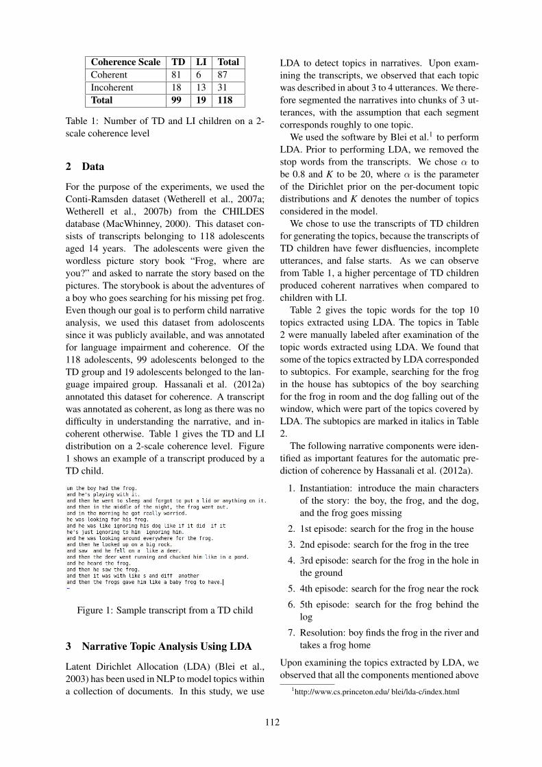
Coherence Scale TD LI TotalCoherent 81 6 87Incoherent 18 13 31Total 99 19 118
Table 1: Number of TD and LI children on a 2-scale coherence level
2 Data
For the purpose of the experiments, we used theConti-Ramsden dataset (Wetherell et al., 2007a;Wetherell et al., 2007b) from the CHILDESdatabase (MacWhinney, 2000). This dataset con-sists of transcripts belonging to 118 adolescentsaged 14 years. The adolescents were given thewordless picture story book “Frog, where areyou?” and asked to narrate the story based on thepictures. The storybook is about the adventures ofa boy who goes searching for his missing pet frog.Even though our goal is to perform child narrativeanalysis, we used this dataset from adoloscentssince it was publicly available, and was annotatedfor language impairment and coherence. Of the118 adolescents, 99 adolescents belonged to theTD group and 19 adolescents belonged to the lan-guage impaired group. Hassanali et al. (2012a)annotated this dataset for coherence. A transcriptwas annotated as coherent, as long as there was nodifficulty in understanding the narrative, and in-coherent otherwise. Table 1 gives the TD and LIdistribution on a 2-scale coherence level. Figure1 shows an example of a transcript produced by aTD child.
Figure 1: Sample transcript from a TD child
3 Narrative Topic Analysis Using LDA
Latent Dirichlet Allocation (LDA) (Blei et al.,2003) has been used in NLP to model topics withina collection of documents. In this study, we use
LDA to detect topics in narratives. Upon exam-ining the transcripts, we observed that each topicwas described in about 3 to 4 utterances. We there-fore segmented the narratives into chunks of 3 ut-terances, with the assumption that each segmentcorresponds roughly to one topic.
We used the software by Blei et al.1 to performLDA. Prior to performing LDA, we removed thestop words from the transcripts. We chose α tobe 0.8 and K to be 20, where α is the parameterof the Dirichlet prior on the per-document topicdistributions and K denotes the number of topicsconsidered in the model.
We chose to use the transcripts of TD childrenfor generating the topics, because the transcripts ofTD children have fewer disfluencies, incompleteutterances, and false starts. As we can observefrom Table 1, a higher percentage of TD childrenproduced coherent narratives when compared tochildren with LI.
Table 2 gives the topic words for the top 10topics extracted using LDA. The topics in Table2 were manually labeled after examination of thetopic words extracted using LDA. We found thatsome of the topics extracted by LDA correspondedto subtopics. For example, searching for the frogin the house has subtopics of the boy searchingfor the frog in room and the dog falling out of thewindow, which were part of the topics covered byLDA. The subtopics are marked in italics in Table2.
The following narrative components were iden-tified as important features for the automatic pre-diction of coherence by Hassanali et al. (2012a).
1. Instantiation: introduce the main charactersof the story: the boy, the frog, and the dog,and the frog goes missing
2. 1st episode: search for the frog in the house
3. 2nd episode: search for the frog in the tree
4. 3rd episode: search for the frog in the hole inthe ground
5. 4th episode: search for the frog near the rock
6. 5th episode: search for the frog behind thelog
7. Resolution: boy finds the frog in the river andtakes a frog home
Upon examining the topics extracted by LDA, weobserved that all the components mentioned above
1http://www.cs.princeton.edu/ blei/lda-c/index.html
112
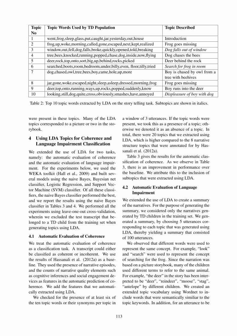
TopicNo
Topic Words Used by TD Population Topic Described
1 went,frog,sleep,glass,put,caught,jar,yesterday,out,house Introduction2 frog,up,woke,morning,called,gone,escaped,next,kept,realized Frog goes missing3 window,out,fell,dog,falls,broke,quickly,opened,told,breaking Dog falls out of window4 tree,bees,knocked,running,popped,chase,dog,inside,now,flying Dog chases the bees5 deer,rock,top,onto,sort,big,up,behind,rocks,picked Deer behind the rock6 searched,boots,room,bedroom,under,billy,even, floor,tilly,tried Search for frog in room7 dog,chased,owl,tree,bees,boy,came,hole,up,more Boy is chased by owl from a
tree with beehives8 jar,gone,woke,escaped,night,sleep,asleep,dressed,morning,frog Frog goes missing9 deer,top,onto,running,ways,up,rocks,popped,suddenly,know Boy runs into the deer10 looking,still,dog,quite,cross,obviously,smashes,have,annoyed Displeasure of boy with dog
Table 2: Top 10 topic words extracted by LDA on the story telling task. Subtopics are shown in italics.
were present in these topics. Many of the LDAtopics corresponded to a picture or two in the sto-rybook.
4 Using LDA Topics for Coherence andLanguage Impairment Classification
We extended the use of LDA for two tasks,namely: the automatic evaluation of coherenceand the automatic evaluation of language impair-ment. For the experiments below, we used theWEKA toolkit (Hall et al., 2009) and built sev-eral models using the naive Bayes, Bayesian netclassifier, Logistic Regression, and Support Vec-tor Machine (SVM) classifier. Of all these classi-fiers, the naive Bayes classifier performed the best,and we report the results using the naive Bayesclassifier in Tables 3 and 4. We performed all theexperiments using leave-one-out cross-validation,wherein we excluded the test transcript that be-longed to a TD child from the training set whengenerating topics using LDA.
4.1 Automatic Evaluation of CoherenceWe treat the automatic evaluation of coherenceas a classification task. A transcript could eitherbe classified as coherent or incoherent. We usethe results of Hassanali et al. (2012a) as a base-line. They used the presence of narrative episodes,and the counts of narrative quality elements suchas cognitive inferences and social engagement de-vices as features in the automatic prediction of co-herence. We add the features that we automati-cally extracted using LDA.
We checked for the presence of at least six ofthe ten topic words or their synonyms per topic in
a window of 3 utterances. If the topic words werepresent, we took this as a presence of a topic; oth-erwise we denoted it as an absence of a topic. Intotal, there were 20 topics that we extracted usingLDA, which is higher compared to the 8 narrativestructure topics that were annotated for by Has-sanali et al. (2012a).
Table 3 gives the results for the automatic clas-sification of coherence. As we observe in Table3, there is an improvement in performance overthe baseline. We attribute this to the inclusion ofsubtopics that were extracted using LDA.
4.2 Automatic Evaluation of LanguageImpairment
We extended the use of LDA to create a summaryof the narratives. For the purpose of generating thesummary, we considered only the narratives gen-erated by TD children in the training set. We gen-erated a summary, by choosing 5 utterances cor-responding to each topic that was generated usingLDA, thereby yielding a summary that consistedof 100 utterances.
We observed that different words were used torepresent the same concept. For example, “look”and “search” were used to represent the conceptof searching for the frog. Since the narration wasbased on a picture storybook, many of the childrenused different terms to refer to the same animal.For example, “the deer” in the story has been inter-preted to be “deer”, “reindeer”, “moose”, “stag”,“antelope” by different children. We created anextended topic vocabulary using Wordnet to in-clude words that were semantically similiar to thetopic keywords. In addition, for an utterance to be
113
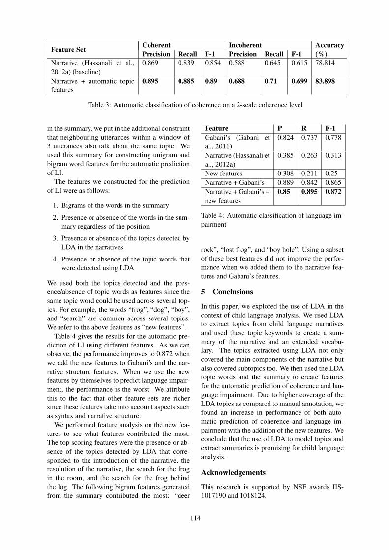
Feature Set Coherent Incoherent Accuracy(%)Precision Recall F-1 Precision Recall F-1
Narrative (Hassanali et al.,2012a) (baseline)
0.869 0.839 0.854 0.588 0.645 0.615 78.814
Narrative + automatic topicfeatures
0.895 0.885 0.89 0.688 0.71 0.699 83.898
Table 3: Automatic classification of coherence on a 2-scale coherence level
in the summary, we put in the additional constraintthat neighbouring utterances within a window of3 utterances also talk about the same topic. Weused this summary for constructing unigram andbigram word features for the automatic predictionof LI.
The features we constructed for the predictionof LI were as follows:
1. Bigrams of the words in the summary
2. Presence or absence of the words in the sum-mary regardless of the position
3. Presence or absence of the topics detected byLDA in the narratives
4. Presence or absence of the topic words thatwere detected using LDA
We used both the topics detected and the pres-ence/absence of topic words as features since thesame topic word could be used across several top-ics. For example, the words “frog”, “dog”, “boy”,and “search” are common across several topics.We refer to the above features as “new features”.
Table 4 gives the results for the automatic pre-diction of LI using different features. As we canobserve, the performance improves to 0.872 whenwe add the new features to Gabani’s and the nar-rative structure features. When we use the newfeatures by themselves to predict language impair-ment, the performance is the worst. We attributethis to the fact that other feature sets are richersince these features take into account aspects suchas syntax and narrative structure.
We performed feature analysis on the new fea-tures to see what features contributed the most.The top scoring features were the presence or ab-sence of the topics detected by LDA that corre-sponded to the introduction of the narrative, theresolution of the narrative, the search for the frogin the room, and the search for the frog behindthe log. The following bigram features generatedfrom the summary contributed the most: “deer
Feature P R F-1Gabani’s (Gabani etal., 2011)
0.824 0.737 0.778
Narrative (Hassanali etal., 2012a)
0.385 0.263 0.313
New features 0.308 0.211 0.25Narrative + Gabani’s 0.889 0.842 0.865Narrative + Gabani’s +new features
0.85 0.895 0.872
Table 4: Automatic classification of language im-pairment
rock”, “lost frog”, and “boy hole”. Using a subsetof these best features did not improve the perfor-mance when we added them to the narrative fea-tures and Gabani’s features.
5 Conclusions
In this paper, we explored the use of LDA in thecontext of child language analysis. We used LDAto extract topics from child language narrativesand used these topic keywords to create a sum-mary of the narrative and an extended vocabu-lary. The topics extracted using LDA not onlycovered the main components of the narrative butalso covered subtopics too. We then used the LDAtopic words and the summary to create featuresfor the automatic prediction of coherence and lan-guage impairment. Due to higher coverage of theLDA topics as compared to manual annotation, wefound an increase in performance of both auto-matic prediction of coherence and language im-pairment with the addition of the new features. Weconclude that the use of LDA to model topics andextract summaries is promising for child languageanalysis.
Acknowledgements
This research is supported by NSF awards IIS-1017190 and 1018124.
114
ReferencesDavid M. Blei, Andrew Y. Ng, and Michael I. Jordan.
2003. Latent dirichlet allocation. the Journal of ma-chine Learning research, 3:993–1022.
Keyur Gabani, Thamar Solorio, Yang Liu, Khairun-nisa Hassanali, and Christine A. Dollaghan. 2011.Exploring a corpus-based approach for detect-ing language impairment in monolingual English-speaking children. Artificial Intelligence inMedicine, 53(3):161–170.
Mark Hall, Eibe Frank, Geoffrey Holmes, BernhardPfahringer, Peter Reutemann, and Ian H. Witten.2009. The WEKA data mining software: An update.ACM SIGKDD Explorations Newsletter, 11(1):10–18.
Khairun-nisa Hassanali, Yang Liu, and ThamarSolorio. 2012a. Coherence in child language nar-ratives: A case study of annotation and automaticprediction of coherence. In Proceedings of WOCCI2012 - 3rd Workshop on Child, Computer and Inter-action.
Khairun-nisa Hassanali, Yang Liu, and ThamarSolorio. 2012b. Evaluating NLP features for au-tomatic prediction of language impairment usingchild speech transcripts. In Proceedings of INTER-SPEECH.
Brian MacWhinney. 2000. The CHILDES project:Tools for analyzing talk, Volume I: Transcription for-mat and programs. Lawrence Erlbaum Associates.
Sam Sahakian and Benjamin Snyder. 2012. Automat-ically learning measures of child language develop-ment. In Proceedings of the 50th Annual Meetingof the Association for Computational Linguistics:Short Papers-Volume 2, pages 95–99. Associationfor Computational Linguistics.
Bryon C. Wallace. 2012. Multiple narrative disentan-glement: Unraveling infinite jest. In Proceeding ofthe 2012 Conference of the North American Chap-ter of the Association for Computational Linguistics:Human Language Technologies, pages 1–10.
Danielle Wetherell, Nicola Botting, and Gina Conti-Ramsden. 2007a. Narrative in adolescent specificlanguage impairment (SLI): a comparison with peersacross two different narrative genres. InternationalJournal of Language & Communication Disorders,42(5):583–605.
Danielle Wetherell, Nicola Botting, and Gina Conti-Ramsden. 2007b. Narrative skills in adolescentswith a history of SLI in relation to non-verbal IQscores. Child Language Teaching and Therapy,23(1):95.
115
Proceedings of the 2013 Workshop on Biomedical Natural Language Processing (BioNLP 2013), pages 116–119,Sofia, Bulgaria, August 4-9 2013. c©2013 Association for Computational Linguistics
Effect of Out Of Vocabulary terms on inferring eligibility criteria for a
retrospective study in Hebrew EHR
Raphael Cohen*
Computer Science Dept.
Ben-Gurion University in the Negev
Michael Elhadad
Computer Science Dept.
Ben-Gurion University in the Negev
1 Background
The Electronic Health Record (EHR) contains
information useful for clinical, epidemiological
and genetic studies. This information of patient
symptoms, history, medication and treatment is
not completely captured in the structured part of
the EHR but is often found in the form of free-
text narrative.
A major obstacle for clinical studies is finding
patients that fit the eligibility criteria of the
study. Using EHR in order to automatically iden-
tify relevant cohorts can help speed up both clin-
ical trials and retrospective studies (Restificar,
Korkontzelos et al. 2013).
While the clinical criteria for inclusion and
exclusion from the study are explicitly stated in
most studies, automating the process using the
EHR database of the hospital is often impossible
as the structured part of the database (age, gen-
der, ICD9/10 medical codes, etc.’) rarely covers
all of the criteria.
Many resources such as UMLS (Bodenreider
2004), cTakes (Savova, Masanz et al. 2010),
MetaMap (Aronson and Lang 2010) and recently
richly annotated corpora and treebanks (Albright,
Lanfranchi et al. 2013) are available for pro-
cessing and representing medical texts in Eng-
lish. Resource poor languages, however, suffer
from lack in NLP tools and medical resources.
Dictionaries exhaustively mapping medical terms
to the UMLS medical meta-thesaurus are only
available in a limited number of languages be-
sides English. NLP annotation tools, when they
exist for resource poor languages, suffer from
heavy loss of accuracy when used outside the
domain on which they were trained, as is well
documented for English (Tsuruoka, Tateishi et
al. 2005; Tateisi, Tsuruoka et al. 2006).
In this work we focus on the problem of clas-
sifying patient eligibility for inclusion in retro-
spective study of the epidemiology of epilepsy in
Southern Israel. Israel has a centralized structure
of medical services which include advanced
EHR systems. However, the free text sections of
these EHR are written in Hebrew, a resource
poor language in both NLP tools and hand-
crafted medical vocabularies.
Epilepsy is a common chronic neurologic dis-
order characterized by seizures. These seizures
are transient signs and/or symptoms of abnormal,
excessive, or hyper synchronous neuronal activi-
ty in the brain. Epilepsy is one of the most com-
mon of the serious neurological disorders (Hirtz,
Thurman et al. 2007).
2 Corpus
We collected a corpus of patient notes from
the Pediatric Epilepsy Unit, an outpatient clinic
for neurology problems, not limited to epilepsy,
in Soroka Hospital. This clinic is the only availa-
ble pediatric neurology clinic in southern Israel
and at the time of the study was staffed by a sin-
gle expert serving approximately 225,000 chil-
dren. The clinical corpus spans 894 visits to the
Children Epilepsy Unit which occurred in 2009
by 516 unique patients. The corpus contains
226K tokens / 12K unique tokens.
∗Supported by the Lynn and William Frankel Center for
Computer Sciences, Ben Gurion University
116
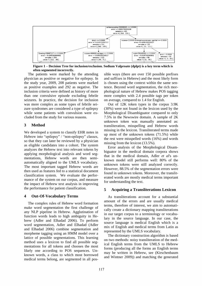
The patients were marked by the attending
physician as positive or negative for epilepsy. In
the study year, 2009, 208 patients were marked
as positive examples and 292 as negative. The
inclusion criteria were defined as history of more
than one convulsive episode excluding febrile
seizures. In practice, the decision for inclusion
was more complex as some types of febrile sei-
zure syndromes are considered a type of epilepsy
while some patients with convulsion were ex-
cluded from the study for various reasons.
3 Method
We developed a system to classify EHR notes in
Hebrew into “epilepsy” / “non-epilepsy” classes,
so that they can later be reviewed by a physician
as eligible candidates into a cohort. The system
analyzes the Hebrew text into relevant tokens by
applying morphological analysis and word seg-
mentations, Hebrew words are then semi-
automatically aligned to the UMLS vocabulary.
The most important tagged Hebrew words are
then used as features fed to a statistical document
classification system. We evaluate the perfor-
mance of the system on our corpus, and measure
the impact of Hebrew text analysis in improving
the performance for patient classification.
4 Out-Of-Vocabulary Terms
The complex rules of Hebrew word formation
make word segmentation the first challenge of
any NLP pipeline in Hebrew. Agglutination of
function words leads to high ambiguity in He-
brew (Adler and Elhadad 2006). To perform
word segmentation, Adler and Elhadad (Adler
and Elhadad 2006) combine segmentation and
morpheme tagging using an HMM model over a
lattice of possible segmentations. This learning
method uses a lexicon to find all possible seg-
mentations for all tokens and chooses the most
likely one according to POS sequences. Un-
known words, a class to which most borrowed
medical terms belong, are segmented in all pos-
sible ways (there are over 150 possible prefixes
and suffixes in Hebrew) and the most likely form
is chosen using the context within the same sen-
tence. Beyond word segmentation, the rich mor-
phological nature of Hebrew makes POS tagging
more complex with 2.4 possible tags per token
on average, compared to 1.4 for English.
Out of 12K token types in the corpus 3.9K
(30%) were not found in the lexicon used by the
Morphological Disambiguator compared to only
7.5% in the Newswire domain. A sample of 2K
unknown token was manually annotated as:
transliteration, misspelling and Hebrew words
missing in the lexicon. Transliterated terms made
up most of the unknown tokens (71.5%) while
the rest were misspelled words (16%) and words
missing from the lexicon (13.5%).
Error analysis of the Morphological Disam-
biguator in the medical domain corpora shows
that in the medical domain, Adler et al's un-
known model still performs well: 80% of the
unknown tokens were still analyzed correctly.
However, 88.5% of the segmentation errors were
found in unknown tokens. Moreover, the translit-
erated words are mostly medical terms important
for understanding the text.
5 Acquiring a Transliterations Lexicon
As transliterations account for a substantial
amount of the errors and are usually medical
terms, therefore of interest, we aim to automati-
cally create a dictionary mapping transliterations
in our target corpus to a terminology or vocabu-
lary in the source language. In our case, the
source language is medical English which is a
mix of English and medical terms from Latin as
represented by the UMLS vocabulary.
The dictionary construction algorithm is based
on two methods: noisy transliteration of the med-
ical English terms from the UMLS to Hebrew
forms (producing all the forms an English terms
may be written in Hebrew, see (Kirschenbaum
and Wintner 2009)) and matching the generated
Figure 1 – Decision Tree for inclusion/exclusion. Sodium Valproate (dplpt) is a key term which is
often segmented incorrectly.
117
transliterations to the unknown Hebrew forms
found in our target corpus. After creating a list of
candidate pairs (Hebrew form found in the cor-
pus and transliterated UMLS concept), we filter
the results to create an accurate dictionary using
various heuristic measures.
The produced lexicon contained 2,507 trans-
literated lemmas with precision of 75%. The ac-
quired lexicon reduced segmentation errors by
50%.
6 Experiments
6.1 Experimental Settings
An SVM classifier was trained using the 200
most common nouns as features. The noun lem-
mas were extracted with the morphological dis-
ambiguator in two settings: naïve setting using
the newswire lexicon and an adapted setting us-
ing the acquired lexicon.
We divided the corpus into training and testing
sets of equal size, we report on the average re-
sults or 10 different divisions of the data.
6.2 Results
The classifier using the baseline lexicon achieved
an average F-Score of 83.6%. With the extended
in-domain transliterations lexicon the classifier
achieves F-Score of 87%, an error reduction of
20%.
We repeated the experiment with decision
trees for visualization for error analysis. With
decision trees we see an improvement from
76.8% to 82.6% F-score. In Figure 1, we see in
the resulting decision tree the most commonly
prescribed medication for epilepsy patients, So-
dium Valproate “depalept” (“דפלפט”). This word
appears in three forms: “depalept”, “b+deplapet”
and “h+depalept”. The acquired lexicon allows
better segmentation of this word thus removing
noise for documents containing the agglutinated
forms.
7 Conclusions
We presented the task of classifying patients’
Hebrew free text EHR for inclusion/exclusion
from a prospective study. Transliterated tokens
are an important feature in medical texts. In lan-
guages with compound tokens this is likely to
lead to segmentation errors.
Using a lexicon adapted for the domain im-
pacts the number of segmentation errors, this
error reduction translates into further improve-
ments when using these data for down the line
applications such as classification.
Creating domain adaptation methods for re-
source-poor languages can positively impact the
use of clinical records in these languages.
Acknowledgments
Adler, M. and M. Elhadad (2006). An
unsupervised morpheme-based hmm for
hebrew morphological disambiguation.
Proceedings of the 21st International
Conference on Computational Linguistics
and the 44th annual meeting of the
Association for Computational
Linguistics, Association for
Computational Linguistics.
Albright, D., A. Lanfranchi, et al. (2013).
"Towards comprehensive syntactic and
semantic annotations of the clinical
narrative." Journal of the American
Medical Informatics Association.
Aronson, A. R. and F. M. Lang (2010). "An
overview of MetaMap: historical
perspective and recent advances." Journal
of the American Medical Informatics
Association 17(3): 229-236.
Bodenreider, O. (2004). "The unified medical
language system (UMLS): integrating
biomedical terminology." Nucleic Acids
Research 32(Database Issue): D267.
Hirtz, D., D. Thurman, et al. (2007). "How
common are the “common” neurologic
disorders?" Neurology 68(5): 326-337.
Kirschenbaum, A. and S. Wintner (2009). Lightly
supervised transliteration for machine
translation. Proceedings of the 12th
Conference of the European Chapter of
the Association for Computational
Linguistics, Association for
Computational Linguistics.
Restificar, A., I. Korkontzelos, et al. (2013). "A
method for discovering and inferring
appropriate eligibility criteria in clinical
trial protocols without labeled data."
BMC Medical Informatics and Decision
Making 13(Suppl 1): S6.
Savova, G. K., J. J. Masanz, et al. (2010). "Mayo
clinical Text Analysis and Knowledge
Extraction System (cTAKES):
architecture, component evaluation and
applications." Journal of the American
Medical Informatics Association 17(5):
507-513.
Tateisi, Y., Y. Tsuruoka, et al. (2006). Subdomain
adaptation of a POS tagger with a small
corpus. Proceedings of the Workshop on
118

Linking Natural Language Processing and
Biology: Towards Deeper Biological
Literature Analysis, Association for
Computational Linguistics.
Tsuruoka, Y., Y. Tateishi, et al. (2005).
"Developing a robust part-of-speech
tagger for biomedical text." Advances in
informatics: 382-392.
119
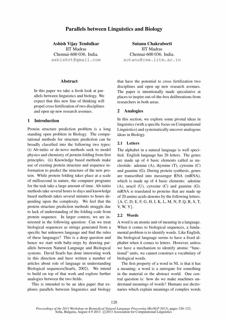
Proceedings of the 2013 Workshop on Biomedical Natural Language Processing (BioNLP 2013), pages 120–123,Sofia, Bulgaria, August 4-9 2013. c©2013 Association for Computational Linguistics
Parallels between Linguistics and Biology
Ashish Vijay TendulkarIIT Madras
Chennai-600 036. [email protected]
Sutanu ChakrabortiIIT Madras
Chennai-600 036. [email protected]
Abstract
In this paper we take a fresh look at par-allels between linguistics and biology. Weexpect that this new line of thinking willpropel cross fertilization of two disciplinesand open up new research avenues.
1 Introduction
Protein structure prediction problem is a longstanding open problem in Biology. The compu-tational methods for structure prediction can bebroadly classified into the following two types:(i) Ab-initio or de-novo methods seek to modelphysics and chemistry of protein folding from firstprinciples. (ii) Knowledge based methods makeuse of existing protein structure and sequence in-formation to predict the structure of the new pro-tein. While protein folding takes place at a scaleof millisecond in nature, the computer programsfor the task take a large amount of time. Ab-initiomethods take several hours to days and knowledgebased methods takes several minutes to hours de-pending upon the complexity. We feel that theprotein structure prediction methods struggle dueto lack of understanding of the folding code fromprotein sequence. In larger context, we are in-terested in the following question: Can we treatbiological sequences as strings generated from aspecific but unknown language and find the rulesof these languages? This is a deep question andhence we start with baby-steps by drawing par-allels between Natural Language and Biologicalsystems. David Searls has done interesting workin this direction and have written a number ofarticles about role of language in understandingBiological sequences(Searls, 2002). We intendto build on top of that work and explore furtheranalogies between the two fields.
This is intended to be an idea paper that ex-plores parallels between linguistics and biology
that have the potential to cross fertilization twodisciplines and open up new research avenues.The paper is intentionally made speculative atplaces to inspire out-of-the-box deliberations fromresearchers in both areas.
2 Analogies
In this section, we explore some pivotal ideas inlinguistics (with a specific focus on ComputationalLinguistics) and systematically uncover analogousideas in Biology.
2.1 LettersThe alphabet in a natural language is well speci-fied. English language has 26 letters. The genesare made up of 4 basic elements called as nu-cleotide: adenine (A), thymine (T), cytosine (C)and guanine (G). During protein synthesis, genesare transcribed into messenger RNA (mRNA),which is made up of 4 basic elements: adenine(A), uracil (U), cytosine (C) and guanine (G).mRNA is translated to proteins that are made upof 20 amino acids denotes by the following letters:{A, C, D, E, F, G, H, I, K, L, M, N, P, Q, R, S, T,V, W, Y}.
2.2 WordsA word is an atomic unit of meaning in a language.When it comes to biological sequences, a funda-mental problem is to identify words. Like English,the biological language seems to have a fixed al-phabet when it comes to letters. However, unlesswe have a mechanism to identify atomic “func-tional” units, we cannot construct a vocabulary ofbiological words.
The first property of a word in NL is that it hasa meaning; a word is a surrogate for somethingin the material or the abstract world. One cen-tral question is: how do we make machines un-derstand meanings of words? Humans use dictio-naries which explain meanings of complex words
120
in terms of simple ones. For machines to use dic-tionaries, we have two problems. The first is, howdo we communicate the meaning of simple words(like “red” or “sad”)? The second is, to under-stand meanings of complex words out of simpleones, we would need the machine to understandEnglish in the first place. The first problem hasno easy solution; there are words whose meaningsare expressed better in the form of images or whencontrasted with other words (“orange” versus “yel-low”). The second problem of defining words interms of others can be addressed using a knowl-edge representation formalism like a semantic net-work. Some biological words have functions thatcannot be easily expressed in terms of functionsof other words. For the other words, we can definethe function (semantics) of a biological word interms of other biological words, leading to a dic-tionary or ontology of such words.
The second property of a word is its Part ofSpeech which dictates the suitability of words totie up with each other to give rise to grammaticalsentences. An analogy can be drawn to valencyof atoms, which is primarily responsible in dictat-ing which molecules are possible and which arenot. Biological words may have Parts of speechthat dictate their ability to group together to formhigher level units like sentences, using the compo-sition of functions which has its analog in compo-sitional semantics. The third property of a wordis its morphology, which is its structure or form.This refers to the sequence of letters in the words.There are systematic ways in which the form of aroot word (like sing) can be changed to give birthto new words (like singing). Two primary pro-cesses are inflection and derivation. This can berelated to mutations in Biology, where we obtain anew sequence or structure by mutating the existingsequences/structures.
3 Concepts
Effective Dimensionality: The Vector SpaceModel (VSM) is used frequently as a formalismin Information Retrieval. When used over a largecollection of documents as in the web, VSM pic-tures the webpages as vectors in a high dimen-sional vector space, where each dimension corre-sponds to a word. Interestingly, thanks to strongclustering properties exhibited by documents, thishigh dimensional space is only sparsely populatedby real world documents. As an example to il-
lustrate this, we would not expect a webpage to si-multaneously talk about Margaret Thatcher, DiegoMaradona and Machine Learning. Thus, more of-ten than not, the space defined by intersection oftwo or more words is empty. The webspace is likethe night sky: mostly dark and few clusters sprin-kled in between. In IR parlance, we say that theeffective dimensionality of the space is much lessthan the true dimensionality, and this fact can beexploited cleverly to overcome “curse of dimen-sionality” and to speed up retrieval. It is worthnoting that the world of biological sequences isnot very different. Of all the sequences that canbe potentially generated, only a few correspond tostable configurations.
Ramachandran plot is used to understand con-straints in protein conformations (Ramachandran,1963). It plots possible φ − ψ angle pairs in pro-tein structures based on the van der Waal radii ofamino acids. It demonstrates that the protein con-formational space is sparse and is concentrated inclusters of a few φ− ψ regions.
3.1 Machine TranslationGenes and mRNAs can be viewed as strings gen-erated from four letters (A,T,C,G for genes andA,U,C,G for mRNAs). Proteins can be viewedas strings generated from twenty amino acids. Inaddition proteins and mRNAs have correspond-ing structures for which we do not even knowthe alphabets. The genes are storing a blue-printfor synthesizing proteins. Whenever the cell re-quires a specific protein, the protein synthesistakes place, in which first the genes encoding thatprotein are read and are transcribed into mRNAwhich are then translated to make proteins withrelevant amino acids. This is similar to writing thesame document in multiple languages so that it canbe consumed by the people familiar to differentlanguages. Here the protein sequence is encodedin genes and is communicated in form of mRNAduring the synthesis process. Another example issequence and structure representations of protein:Both of them carry the same information specifiedin different forms.
3.2 Evolution of LanguagesLanguage evolves over time to cater to evolutionin our communication goals. New concepts orig-inate which warrant revisions to our vocabulary.The language of mathematics has evolved to makecommunication more precise. Sentence structures
121
evolve, often to address the bottlenecks faced bynative speakers and second language learners. En-glish, for example, has gone out of fashion. Thusthere is a survival goal very closely coupled to theenvironment in which a language thrives that dic-tates its evolution. The situation is not very differ-ent in biology.
Scientific community believes that the life onthe Earth started with prokaryotes1 and evolvedinto eukaryotes. Prokaryotes inhibited earth fromapproximately 3-4 Billion years ago. About 500million years ago, plant and fungi colonized theEarth. The modern human came into existencesince 250,000 years. At a genetic level, newgenes were formed by means of insertion, dele-tion and mutation of certain nucleotide with othernucleotides.
3.3 Garden Path Sentences
English is replete with examples where a smallchange in a sentence leads to a significant changein its meaning. A case in point is the sen-tence “He eats shoots and leaves”, whose meaningchanges drastically when a comma is inserted be-tween “eats” and “shoots”. This leads to situationswhere the meaning of a sentence cannot be com-posed by a linear composition of the meanings ofwords. The situation is not very different in biol-ogy, where the function of a sequence can changewhen any one element in the sequence changed.
3.4 Text and background knowledge neededto understand it
Interaction between the “book” and the reader isessential to comprehension; so language under-standing is not just sophisticated modeling of in-teraction between words, sentences and discourse.Similarly the book of life (the gene sequence) doesnot have everything that is needed to determinefunction; it needs to be read by the reader (playedby the CD player). This phenomenon is similarto protein/ gene interaction. Proteins/genes pos-sess binding sites, that is used to bind other pro-teins/genes to form a complex, which carry out thedesired function in the biological process.
3.5 Complexity of Dataset
Several measures have been proposed in the con-text of Information Retrieval and Text Classifica-tion which aim at capturing the complexity of a
1http://www.wikipedia.org
dataset. In unsupervised domains, a high clus-tering tendency indicates a low complexity anda low clustering tendency corresponds to a situ-ation where the objects are spread out more orless uniformly in space. The latter situation cor-responds to high complexity. In supervised do-mains, a dataset is said to be complex if objectsthat are similar to each other have same categorylabels. Interestingly, these ideas may apply in ar-riving at estimates of structure complexity. In par-ticular, weak structure function correspondenceswould correspond to high complexity.
3.6 Stop words (function words) and theirrole in syntax
Function words such as articles, prepositions playan important role in understanding natural lan-guages. On the same note, function words existin Biology and they play various important rolesdepending on the context. For example, Proteinstructures are made up of secondary structures.Around 70% of these structures are α-helix andβ-strands which repeat in functionally unrelatedproteins. Based on this criterion, α-helix and β-strands can be categorized as functional words.These secondary structures are important in form-ing protein structural frame on which functionalsites can be mounted. At genomic level, as muchas 97% of human genome does not code for pro-teins and hence termed as junk DNA. This is an-other instance of function word in Biology. Scien-tists are realizing off late some important functionsof these junk DNA such as their role in alternativesplicing.
3.7 Natural Language GenerationNatural Language Generation (NLG) is com-plementary to Natural Language Understanding(NLU), in that it aims at constructing natural lan-guage text from a variety of non-textual repre-sentations like maps, graphs, tables and tempo-ral data. NLG can be used to automate routinetasks like generation of memos, letters or simula-tion reports. At the creative end of the spectrum,an ambitious goal of NLG would be to composejokes, advertisements, stories and poetry. NLGis carried out in four steps: (i) macroplanning;(ii)microplanning; (iii) surface realization and (iv)presentation. Macroplanning step uses RhetoricalStructure Theory (RST), which defines relationsbetween units of text. For example, the relationcause connects the two sentences: “The hotel was
122
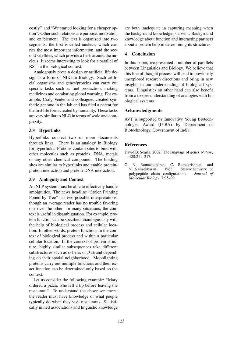
costly.” and “We started looking for a cheaper op-tion”. Other such relations are purpose, motivationand enablement. The text is organized into twosegments; the first is called nucleus, which car-ries the most important information, and the sec-ond satellites, which provide a flesh around the nu-cleus. It seems interesting to look for a parallel ofRST in the biological context.
Analogously protein design or artificial life de-sign is a form of NLG in Biology. Such artifi-cial organisms and genes/proteins can carry outspecific tasks such as fuel production, makingmedicines and combating global warming. For ex-ample, Craig Venter and colleagues created syn-thetic genome in the lab and has filed a patent forthe first life form created by humanity. These tasksare very similar to NLG in terms of scale and com-plexity.
3.8 HyperlinksHyperlinks connect two or more documentsthrough links. There is an analogy in Biologyfor hyperlinks. Proteins contain sites to bind withother molecules such as proteins, DNA, metalsor any other chemical compound. The bindingsites are similar to hyperlinks and enable protein-protein interaction and protein-DNA interaction.
3.9 Ambiguity and ContextAn NLP system must be able to effectively handleambiguities. The news headline “Stolen PaintingFound by Tree” has two possible interpretations,though an average reader has no trouble favoringone over the other. In many situations, the con-text is useful in disambiguation. For example, pro-tein function can be specified unambiguously withthe help of biological process and cellular loca-tion. In other words, protein functions in the con-text of biological process and within a particularcellular location. In the context of protein struc-ture, highly similar subsequences take differentsubstructures such as α-helix or β-strand depend-ing on their spatial neighborhood. Moonlightingproteins carry out multiple functions and their ex-act function can be determined only based on thecontext.
Let us consider the following example: “Maryordered a pizza. She left a tip before leaving therestaurant.” To understand the above sentences,the reader must have knowledge of what peopletypically do when they visit restaurants. Statisti-cally mined associations and linguistic knowledge
are both inadequate in capturing meaning whenthe background knowledge is absent. Backgroundknowledge about function and interacting partnersabout a protein help in determining its structures.
4 Conclusion
In this paper, we presented a number of parallelsbetween Linguistics and Biology. We believe thatthis line of thought process will lead to previouslyunexplored research directions and bring in newinsights in our understanding of biological sys-tems. Linguistics on other hand can also benefitfrom a deeper understanding of analogies with bi-ological systems.
Acknowledgments
AVT is supported by Innovative Young Biotech-nologist Award (IYBA) by Department ofBiotechnology, Government of India.
ReferencesDavid B. Searls. 2002. The language of genes Nature,
420:211–217.
G. N. Ramachandran, C. Ramakrishnan, andV. Sasisekharan. 1963. Stereochemistry ofpolypeptide chain configurations Journal ofMolecular Biology, 7:95–99.
123

Author Index
Ansari, Sam, 80Aronson, Alan, 102
Bedore, Lisa, 89Bejan, Cosmin, 10Bethard, Steven, 18Bobic, Tamara, 80Bretschneider, Claudia, 27
Chakraborti, Sutanu, 120Cohen, Kevin, 1, 72Cohen, Raphael, 116Conway, Mike, 36
Dell’Orletta, Felice, 45Demner-Fushman, Dina, 54Dligach, Dmitriy, 18Duneld, Martin, 36
Elhadad, Michael, 116
Fiszman, Marcelo, 54Fluck, Juliane, 80
Ginter, Filip, 63Glauser, Tracy A., 1
Hammon, Matthias, 27Hassanali, Khairun-nisa, 111Henriksson, Aron, 36Hoeng, Julia, 80Hofmann-Apitius, Martin, 80Holland, Katherine D., 1
Iglesias, Aquiles, 89
Jimeno Yepes, Antonio, 102
Kaewphan, Suwisa, 63Kilicoglu, Halil, 54Klenner, Alexander, 80Kvist, Maria, 36
Lin, Chen, 18Liu, Yang, 89, 111
Madan, Sumit, 80
Matykiewicz, Pawel, 1Miller, Timothy, 18Montemagni, Simonetta, 45Montes, Manuel, 89Mork, James, 102
Peitsch, Manuel, 80Pena, Elizabeth, 89Pestian, John, 1Pradhan, Sameer, 18
Ramirez-de-la-Rosa, Gabriela, 89
Savova, Guergana, 18Skeppstedt, Maria, 36, 98Solorio, Thamar, 89, 111Standridge, Shannon M., 1
Temnikova, Irina, 72Tendulkar, Ashish, 120
Van de Peer, Yves, 63Van Landeghem, Sofie, 63Venturi, Giulia, 45Verspoor, Karen M., 1
Wurfel, Mark, 10
Yetisgen-Yildiz, Meliha, 10
Zillner, Sonja, 27
125