PNNL-19124

Prepared for the U.S. Department of Energy under Contract DE-AC05-76RL01830

Biomass Energy for Transport and Electricity: Large Scale Utilization Under Low CO2 Concentration Scenarios P Luckow JJ Dooley MA Wise SH Kim January 2010

DISCLAIMER This report was prepared as an account of work sponsored by an agency of the United States Government. Neither the United States Government nor any agency thereof, nor Battelle Memorial Institute, nor any of their employees, makes any warranty, express or implied, or assumes any legal liability or responsibility for the accuracy, completeness, or usefulness of any information, apparatus, product, or process disclosed, or represents that its use would not infringe privately owned rights. Reference herein to any specific commercial product, process, or service by trade name, trademark, manufacturer, or otherwise does not necessarily constitute or imply its endorsement, recommendation, or favoring by the United States Government or any agency thereof, or Battelle Memorial Institute. The views and opinions of authors expressed herein do not necessarily state or reflect those of the United States Government or any agency thereof. PACIFIC NORTHWEST NATIONAL LABORATORY operated by BATTELLE for the UNITED STATES DEPARTMENT OF ENERGY under Contract DE-AC05-76RL01830 Printed in the United States of America Available to DOE and DOE contractors from the Office of Scientific and Technical Information,

P.O. Box 62, Oak Ridge, TN 37831-0062; ph: (865) 576-8401 fax: (865) 576-5728

email: reports@adonis.osti.gov Available to the public from the National Technical Information Service, U.S. Department of Commerce, 5285 Port Royal Rd., Springfield, VA 22161

ph: (800) 553-6847 fax: (703) 605-6900

email: orders@ntis.fedworld.gov online ordering: http://www.ntis.gov/ordering.htm

This document was printed on recycled paper.

(9/2003)

PNNL-19124

Biomass Energy for Transport and Electricity: Large Scale Utilization Under Low CO2 Concentration Scenarios P Luckow JJ Dooley MA Wise SH Kim January 2010 Prepared for the U.S. Department of Energy under Contract DE-AC05-76RL01830 Pacific Northwest National Laboratory Richland, Washington 99352

3

Abstract

This paper examines the potential role of large scale, dedicated commercial biomass energy systems under global climate policies designed to stabilize atmospheric concentrations of CO2 at 400ppm and 450ppm. We use an integrated assessment model of energy and agriculture systems to show that, given a climate policy in which terrestrial carbon is appropriately valued equally with carbon emitted from the energy system, biomass energy has the potential to be a major component of achieving these low concentration targets. The costs of processing and transporting biomass energy at much larger scales than current experience are also incorporated into the modeling. From the scenario results, 120-160 EJ/year of biomass energy is produced by midcentury and 200-250 EJ/year by the end of this century. In the first half of the century, much of this biomass is from agricultural and forest residues, but after 2050 dedicated cellulosic biomass crops become the dominant source.

A key finding of this paper is the role that carbon dioxide capture and storage (CCS) technologies coupled with commercial biomass energy can play in meeting stringent emissions targets. Despite the higher technology costs of CCS, the resulting negative emissions used in combination with biomass are a very important tool in controlling the cost of meeting a target, offsetting the venting of CO2 from sectors of the energy system that may be more expensive to mitigate, such as oil use in transportation. The paper also discusses the role of cellulosic ethanol and Fischer-Tropsch biomass derived transportation fuels and shows that both technologies are important contributors to liquid fuels production, with unique costs and emissions characteristics. Through application of the GCAM integrated assessment model, it becomes clear that, given CCS availability, bioenergy will be used both in electricity and transportation.

Key Words Bioenergy; carbon dioxide capture and storage; climate change; greenhouse gas emissions mitigation; electricity generation sector; transportation sector

4

1.0 Introduction and Motivation Since the start of the Industrial Revolution, the mean global concentration of carbon dioxide (CO2) has risen from 280 ppm to currently more than 385 ppm as a result of fossil fuel use and land use changes, and anthropogenic emissions are accelerating (IPCC 2007a ; Raupach et al. 2007; Tans 2009). In order to stabilize atmospheric concentrations of CO2 annual emissions must peak and decline thereafter as described in Wigley et al., 1995. Paltsev et al (2007) provide a useful overview of the broad suite of potential emissions reduction polices that have been put forward to address climate change. Recently significant attention has been focused on the challenge inherent at stabilizing atmospheric concentrations of CO2 at levels that are slightly above today’s level of 385 ppm (IPCC 2007a ; Matthews et al. 2007; Calvin et al. 2009). It is clear that to meet increasingly close targets such as 400ppm to 450ppm CO2 concentrations, significant changes will have to be made to the global energy system. The focus of this paper is to examine the potential role of large scale, dedicated commercial biomass energy systems under stringent climate policies designed to stabilize atmospheric concentrations of CO2 at 400ppm and 450ppm. Currently, biomass provides approximately 10% of global primary energy supply or approximately 46EJ/year (IPCC 2007b). In their survey of 17 long term energy supply scenarios, Berndes et. al. (2003) demonstrate that there is a widely held expectation that bioenergy will play an even larger role in the future (i.e., 100EJ/year to 400EJ/year by 2050 across the literature they surveyed. More recently, the US Climate Change Science Program (2007) presented analyses from three different integrated assessment modeling groups across a range of potential climate policies that showed global contributions from commercial biomass of between just under 100EJ/year to more than 250EJ/year by the end of this century depending on the stringency of the modeled climate policy. A recent integrated modeling study by Wise et al. (2009a) that utilized the same model employed in this analysis demonstrated the importance of land use policy if large scale biomass energy production is to be an effective (and efficient) part of humanity’s emissions mitigation portfolio. A clear result of that work was that a climate policy that encouraged biomass in the energy system but did not account for indirect emissions from land use associated with growing biomass would lead to runaway clearing of land and therefore be counterproductive in terms of limiting CO2 emissions. However, another result of the study was that, in a policy where the carbon in land is valued equally with the carbon emitted by the energy system – bioenergy, including purpose grown crops, could be a major component of CO2 mitigation. And when bioenergy is used in conjunction with CO2 capture and storage (CCS), it may be a key technology in achieving low CO2 concentrations. In this paper, we assume that this type of land use policy is in place so that any biomass produced is not counterproductive. In analyzing the uses of biomass under a stringent climate policy, we also detail the factors and additional costs involved in very large scale biomass production and distribution, levels which are very different from current experience. However, the presence of a strict climate policy is very different from current experience. The relative costs of technologies and processes that are not economically competitive now can change dramatically under a policy that places an economic penalty on CO2 emissions. With the land use policy and the costs of large scale biomass production and use accounted for, in this paper we examine the potential role of large scale, commercial biomass energy systems under stringent climate policies, with a specific focus on exploring where biomass would be used in the energy system. Much of the discussion of near term expansion of biomass energy has been for producing liquid fuels, especially for transportation (Lindfeldt et al. 2008; van Vliet et al. 2009). More recently, longer-term studies of climate policies have seen a shift to using biomass coupled with CCS to make electricity (see for example Calvin, et al, 2009; IPCC 2007b). We demonstrate here that there is no one winner for the use of biomass. We show how climate policies and technology assumptions - especially the availability of CCS technologies - affect the decisions made about where the biomass is used in the energy system.

5

2.0 Modeling Large-Scale Biomass Production and Use Under a climate policy, biomass energy could provide an attractive alternative to fossil fuels, due to photosynthesis of CO2 as it is grown. Biomass energy could be used in several places throughout the energy system, and in some applications may also be used in conjunction with CO2 capture and storage (CCS). When biomass is used in electricity generation, nearly all the CO2 can be captured. In contrast, when biomass is used to make liquid transportation fuels, much of the CO2 is vented at the end use or vehicle tailpipe. Only what is not converted to a fuel in the refinery may be captured, though typically this may be as high as 50% (Lindfeldt et al. 2008; van Vliet et al. 2009). However, this liquid biofuel burned could be offsetting the use of fossil fuels, so it is still a net gain in terms of CO2 emissions. Analyzing where the biomass would be used in the energy system requires a model which considers the economics of biomass technologies and all other fossil, nuclear, renewable, and other technologies in an integrated fashion. But while biomass energy could provide an attractive alternative to fossil fuels in the energy system, its production on a large scale has profound and complex implications for terrestrial systems and the CO2 contained in them (see Wise et al., 2009a). The large scale growth of biomass crops on biomass plantations requires dedicated land. Biomass crops have to compete economically for land with food crops, forests, and other managed and unmanaged land uses. And, critically, the terrestrial CO2 emissions from land use change must be considered for biomass energy to make a positive contribution to emissions mitigation.

2.1 Integrated Assessment Modeling of Biomass Energy: the GCAM Model

The Global Change Assessment Model (GCAM) integrated assessment model, developed at the Pacific Northwest National Laboratory is used to provide the quantitative background for this study. GCAM is the successor to the MiniCAM model (Kim et al. 2006). GCAM models the energy and industrial system, including land use, in an economically consistent global framework. GCAM explicitly models markets and solves for equilibrium prices in energy, agriculture and other land uses, and emissions. GCAM is a long-term model, operating over a projected time horizon from today through 2095. Regional detail is included for 14 distinct regions: the United States, Canada, Western Europe, Japan, Australia & New Zealand, Former Soviet Union, Eastern Europe, Latin America, Africa, Middle East, China and the Asian Reforming Economies, India, South Korea, and Rest of South & East Asia. A thorough description of the how GCAM model the energy production, transformation, and demand systems are provided in Clarke et al (2009). A key feature of GCAM is that it goes beyond modeling the energy systems and incorporates a fully-integrated model of agriculture and land use. A complete description of the GCAM modeling of agriculture and land use is provided in (Wise et al. 2009a), and the key factors related to biomass will be highlighted here. In GCAM, energy, agriculture, forestry, and land markets are integrated, along with unmanaged ecosystems and the terrestrial carbon cycle. Biomass production depends on the availability and character of land resources, technology options for production, and competing land use options. GCAM determines the demands for and production of products originating on the land, the prices of these products, the allocation of land to competing ends, the rental rate on land, and the carbon stocks and flows associated with land use. Land is allocated between alternative uses based on expected profitability, which in turn depends on the productivity of the land-based product (e.g. mass of harvestable product per

6

ha), product price, and non-land costs of production (labor, fertilizer, etc.). The productivity of land-based products grows over time based on future estimates of crop productivity change. Stocks of terrestrial carbon are modeled in each of the GCAM regions based upon data presented in IPCC 2001 and is further distributed among fifteen different reservoir types: unmanaged forests, other unmanaged land, managed forests, nine food and fiber crop types, bioenergy crops, pasture, and non-arable land. This is a critical aspect of the GCAM’s modeling that is of particular relevance to the subject of large scale bioenergy production as the growing and harvesting of dedicated biomass production on the scales considered here will require large areas of land (Brown et al. 1998). Significant fluxes of carbon can result from changes in land-use such as when forests are cleared to create additional crop land. The GCAM specifically models this kind of feedback which reflects a real world constraint as policy should be designed to avoid or minimize these inadvertent and potentially large scale pulses of carbon associated with land-use change (Rosenberg et al. 2005; Wise et al. 2009a).

2.2 Modeling Bioenergy Resources in GCAM In addition to bioenergy from modern biomass commercial methods described below, GCAM considers and models traditional biomass energy, municipal solid waste energy, and energy from agricultural and forest residues. In a historical context, it is instructive to consider traditional biomass a first generation biomass, waste and residue biomass as second generation biomass, and dedicated cellulosic biomass crops as third generation biomass (Dooley 2001). While, first generation biomass goes back to the dawn of man and second generation biomass has long been part of industrial society, third generation biomass has yet to emerge on a large scale. 1 Traditional or first generation biomass consists of straw, dung, fuel wood and other energy forms that are utilized in an unrefined state in the traditional, largely unmarketed sectors of an economy. The IPCC (IPCC 2007b) estimates traditional first generation biomass could represent as much as 30EJ/year, largely concentrated in developing nations. We will not focus on traditional biomass here as it is not a major factor in land use and is assumed to be less prominent as regional incomes rise. In today’s economy, a broad set of second generation biomass feedstocks are currently consumed in the modern commercial energy sector that make use of the energy content of byproducts of another activity such as agricultural residues, forestry residues and municipal solid waste (MSW). IPCC (2007) estimates that 6 EJ/year of biomass energy from crop and forestry residues are used in the commercial energy sector including diverse feedstocks such as black liquor in the pulp and paper industry, wood chips, bark, sawdust from forest product facilities, and oat and rice husks in process heat boilers. Crop and forestry residues are predominantly directly combusted in air to provide process heat (IPCC 2007b). A relatively small but growing use for crop and forestry residues is to produce electricity (in 2007 this accounted for less that 1% of electricity generation in the U.S.) either in dedicated biomass facilities or in facilities that co-fire the biomass with another energy resource most commonly coal (RRI 2009). IPCC (2007) suggests that municipal solid waste currently contributes perhaps another 1 EJ/year to global energy production. In looking forward with the GCAM, the availability of second generation bioenergy from byproduct feedstocks is projected to continue and the theoretical potential of this second generation bioenergy resources is a function of the underlying production of primary products (e.g., the amount of corn grown impacts the availability of corn stover for energy production). Specifically in the GCAM,

1 According to RRI 2009, there are no commercial electricity plants in the U.S. that make use of third generation bioenergy crops although there have been a few small demonstration projects.

7

• Forest products, timber harvesting residue and mill residue are considered. For timber harvesting, the residue retention parameter is estimated at 2 t/ha, calculated by Pannkuk and Robichaud (2003). Timber harvesting residue consists of tree tops, slash, and branches. We assume that all economically exploitable mill residues such as wood scraps, sawdust, and recovered pulping liquors are used.

• For municipal solid waste, the GCAM uses the methodology detailed in Gregg, 2009. The salient points of the Gregg (2009) methodology are as follows. The amount of discarded biomass available for energy is a function of what proportion of a country’s population has access to MSW collection services, how much of waste enters the was stream (rather than being lost, littered, or recovered by the consumer), and, finally, the proportion of the waste stream recovered by the municipality, either by composting or recycling. These proportions are implemented as logistic functions based on per capita GDP, varying from 0 to 1. The total amount of discarded biomass is multiplied by each of these parameters to obtain an estimate for the amount of collected biomass.

• To determine the supply of agricultural biomass residue that can be used for energy production in future years, the GCAM employs the methodology developed by Gregg (2009). The key aspects of this modeling approach are based upon more detailed properties of specific crops. For example, harvest index, water content, and residue energy are estimated for each crop. The harvest index is the ratio of the harvested crop to the total aboveground biomass, and – adjusted for water content- represents the total amount of aboveground crop reside. Not all of this residue is harvestable; some must remain uncollected on the soil to maintain nutrient levels and prevent erosion thereby sustaining the productivity of the land. This amount, represented by a Residue Retention Parameter, is crop-specific, assumed to be 70% for major grain and oil crops, such as corn and wheat, or a maximum residue recovery of 30%. The maximum residue recovery factor for rice is estimated to be 75%.

GCAM models the production of dedicated third generation biomass crops explicitly as part of the economic competition for competing uses of land. While a variety of crops could potentially be grown as bioenergy feedstocks, in this analysis we assume that a representative cellulosic bioenergy crop, based on switchgrass, can be grown in any region, although the productivity of this purpose-grown bioenergy crop is based on region-specific climate and soil characteristics and varies by a factor of three across the GCAM regions (see Wise et al. 2009b for specific assumptions). The extent to which these second and third generation bioenergy resources are utilized is a function of the cost of collection and transport and their overall price competitiveness compared to other energy resources which is significantly influenced by the imposition of a climate policy and is something that will be explored in more detail later. For example, the decision to utilize MSW in the energy sector within the GCAM is economic; as energy prices rise, more MSW will be collected and utilized.

2.3 Accounting for the Infrastructure need to Process and Utilize 100s of EJ/year of Bioenergy

Large scale production and consumption of commercial biomass energy is very different from current experience. The economics of biomass energy today are often such that only small scale projects with a cheap local source of residue of waste biomass are viable. But a climate policy that makes fossil fuels more expensive to use, along with continued technological improvement in biomass growth and use, may be a game-changer. Therefore, our modeling needs to consider the costs of growing, collecting, processing, and transporting biomass that would be incurred if it were used at the kind of large scales that coal is used today. Our goal is to be conservatively high in these costs in order to avoid overstating the potential (or conversely, understating the costs) of large scale biomass deployment under a climate policy.

8

In the future, there will likely remain situations in which there is a local supply of biomass that does not have to be processed and transported before using in an energy facility. However, in an effort to be conservative in our assessment of the potential for bioenergy, we assume here in the GCAM modeling that all commercial biomass generated in the future must undergo a pelletization process in order to increase the energy density of the raw biomass and facilitate long distance transportation (Wolf et al. 2006). Within the GCAM, this is done by assessing a cost for collecting and transporting biomass to a processing facility and converting the raw material to pellets. Based on data provided by van Vliet et al. (2009), an average biomass processing cost of 1.87 2005$/GJ was used. The vast majority (85%) of this additional cost is incurred during the pelletization process, with the remainder resulting from short-distance transport costs to collect the biomass. This pelletization process, which is applicable to baled switchgrass as well as woody biomass, results in a feedstock that is on the order of 10mm in average particle size, with a density of 650 kg/m3 and a heating value of 19.5 GJ/dry tonne (Hamelinck et al. 2005). The pelletization process also removes most of the water content, which helps control decomposition and spoilage (Hamelinck et al, 2005). Based upon the work of Hamelinck et al., 2005 and as depicted in Figure 1, we are also assuming that this pelletization process happens at a fairly disaggregated level close to the point of production of the bioenergy crops and that a certain amount of drying and densification can be integrated into the actual harvesting of the bioenergy crop (e.g., baling for a crop like switch grass or chipping of woody feedstocks). A key insight of the work of these authors is that a bioenergy production system organized in this fashion should exhibit economies of scale that should increase as the bioenergy crop moves through this production chain as a water content of the original fuel is being decreased and densification is being increased at each step.2

2 A central premise of the research presented in this paper is a re-examination of the conventional orthodoxy that large scale bioenergy production will be very expensive and or impractical due to what are seen as inherent diseconomies of scale associated with the collection and preparation of bioenergy crops. For example RRI (2009) and IPCC (2005) both assert that biomass power plants are likely to remain small (RRI says likely less than 50MW in size) and have lower energy efficiencies and higher capital costs than coal-fired power plants. Further, there are a number of analyses that posit that the economics of biomass energy production will be negatively impacted by inherent attributes of bioenergy feedstocks. A number of analyses note the lower energy density of bioenergy crops when compared to coal. Williams et al. (2009) and RRI (2009) also claim that the economic competitiveness of bioenergy facilities will suffer because there is no dedicated infrastructure for moving bioenergy crops to large central energy processing stations. Another common refrain in the literature about limits to the large scale use of biomass are assumptions such as those employed by Larson et al. 2009 that only lands currently not being used for food (i.e., in the U.S. this would include lands in the Crop Reserve Program) or on degraded or abandoned lands can be used for growing third generation bioenergy (Larson et al. 2009). In this paper, we reject the underlying assumptions about future bioenergy production and conversion and are therefore not bound by the resulting ex ante assumptions about the lack of economic competitiveness of large scale bioenergy production (and in particular reject the assertion that bioenergy will not be competitive in a future world that assigns a significant penalty for freely venting anthropogenic CO2 to the atmosphere).

9

Figure 1: Illustration of a biomass production, processing, and distribution system. Reproduced from Hamelinck et al 2007 One more key assumption about biomass production within GCAM relates to shipping the resulting pelletized bioenergy fuel over long distances. To be conservative, the GCAM adds a further transportation expense of $0.31 2005$/GJ for all biomass created (van Vliet et al. 2009).3 This cost is intended to reflect the cost of transporting the pelletized biomass via large ocean-going Suezmax bulk carriers, and contributes to a net cost adder of 2.18 2005$/GJ for biomass processing and transport. This compares to a cost of 1.33 2005$/GJ for producing and delivery of coal (Edwards et al. 2006), less expensive due to coal’s high energy density and low processing requirements. Again, although it would not be necessary to transport all of the biomass produced over long distances, we are purposely being conservative about the costs. In addition, the existence of a large market for biomass would create incentives for producers to bypass local consumers and sell into the larger market, so the higher cost may be relevant even for local use.

2.4 Modeling Biomass Consumption and Use in the Energy System

Biomass is a versatile form of energy which, much like coal, can be burned directly or be converted in other forms of useful energy such as liquid fuels, electricity, methane, and hydrogen. Unlike fossil fuels, the CO2 in sustainably-grown biomass has been recently taken out of the atmosphere, so biomass energy is often considered a carbon-neutral fuel. However, biomass is a still a hydrocarbon fuel, and CO2 is released when it is burned or converted, just like with fossil fuels. As a consequence, a climate policy would place the same economic incentives to avoid the CO2 emissions from biomass fuels as it would fossil fuels. 3 This assumption is “conservative” in the sense that for many parts of the world large biomass production and consumption could happen within the same region and therefore might not need to be transported long distances. By assuming that all biomass bears this cost, the cost of biomass is increased and consumption is decreased.

10

In this study, we focus on technologies to convert biomass into liquid transportation fuels and electricity. We also study energy systems that would incorporate CCS technologies to reduce CO2 venting from these biomass technologies under a climate policy. Although we do not focus here on using biomass to produce gas and hydrogen, these technology options are included in the GCAM and will be seen in some of the results.

2.4.1 Liquid Fuels from Biomass Biofuels could play a major role in the refined liquids sector for providing transportation with a low-carbon fuel. While at the point of use biofuels emit essentially the same about of CO2 as their fossil fuel based counterparts at the vehicle tailpipe, they absorb that CO2 while growing and feedstocks will be continually replanted (McKendry 2002). With biomass being refined from feedstocks at efficiencies near 50% (van Vliet et al. 2009), there is a substantial fraction of the lifecycle emissions that can be captured at the refinery. For this study, we model two distinct technologies for producing liquid fuels from biomass; cellulosic ethanol and Fischer-Tropsch. Ethanol is produced from lignocellulose through saccharification and fermentation through the use of specialized designed enzymes. In producing ethanol from biomass feedstocks, less than half of the carbon initially embedded in the feedstock makes it to the ethanol product. The remainder is either vented to the atmosphere, or may be captured with CCS. A substantial fraction (26%) of high-purity CO2 is released at the scrubber vent, a result of fermentation (Aden et al. 2002). The remainder is in combustion exhaust, where biomass derived byproducts are burned to drive a boiler. These emissions are more dilute, and are assumed to be more expensive to capture. 4 The Fischer-Tropsch (FT) process is a chemical reaction that converts a synthesis gas to liquid fuels. This process is not unique to biofuels; it can be used for coal-to-liquids or gas-to-liquids, and has been done so in the past by countries with an abundance of coal or gas, but lacking in oil resources (van Dyk et al. 2006; Chedid et al. 2007). The FT process results in a relatively large (81.8%) high purity stream of CO2 coming off of the syngas. The syngas is “cleaned” of this CO2 regardless of whether or not CCS is used, to improve the reaction (Dooley et al. 2009; van Vliet et al. 2009). There is a further low purity CO2 stream created from combustion of tail gas. CCS is assumed to apply to the FT process independent of the fuel used, and thus in this analysis coal-to-liquids with CCS will be considered alongside biomass liquids with CCS, and have similar carbon abatement costs. Here we assume CCS costs of $10.67 and $56.26 (2005$/tCO2), for the high and low purity streams respectively (Dooley et al. 2009). Note that the produced cellulosic ethanol is assumed to have relatively lower costs than Fischer-Tropsch, but that Fisher-Tropsch has a much higher percentage of its CO2 that is released in a high-purity stream with a corresponding lower cost of CCS. Costs and efficiencies of ethanol and FT refined liquids, as well as the potential capture fractions are summarized in Table 1. It is assumed for this study that the parameters shown here pertain to the year 2020, and there is a gradual improvement to the end of the century.

4 To a first order approximation, the cost of CO2 capture scales with the concentration CO2 in the flue gas or process stream from which it is being separated from. The lower the concentration of CO2, the higher the per tonCO2 cost of capture tends to be (IPCC 2005).

11

Table 1: Refined Liquids Technology Inputs

Efficiency

Baseline Non-energy Cost (2005$/GJ)

High-Purity CCS Cost Adder (2005$/GJ)

All-capturable CCS Cost Adder ($2005/GJ)

High Purity CCS capture fraction

All-capturable CCS capture fraction

Ethanol 48.6% 7.06 1.85 8.29 26.0% 99.2% Fischer-Tropsch 51.0% 9.84 2.53 4.19 81.8% 98.1%

2.4.2 Electricity from Biomass Many studies (Brown et al. 2009; Research Reports International 2009; Williams et al. 2009) show dramatically higher costs for biomass fired powerplants than for coal plants with the same technology because they assume the plants themselves must be smaller due to limited biomass availability, and thus do not benefit from economies of scale. Because we are incorporating the costs for processing and transporting biomass to be used at large scales, we do not need to make that assumption in this study. That is, we can assume that biomass powerplants will be as large as coal powerplants. However, we do assume a slightly increased cost of biomass-fired power plants as compared to coal power plants of about 3%, due to bulk materials handling and the lower energy density of biomass as compared to coal (see Table 2) (Rhodes et al. 2008; van Vliet et al. 2009).

Table 2: Cost and Efficiency assumptions: Biomass and Coal IGCC power plants in Year 2020

EfficiencyCapital Cost ($/kW)

Fixed O&M ($/kW/yr)

Variable O&M ($/MWh)

Coal IGCC 42.6% 1694 36.5 2.76Coal IGCC (CCS) 36.4% 2233 41.9 5.06Biomass IGCC 41.6% 1745 37.5 2.80Biomass IGCC (CCS) 36.4% 2247 42.1 4.76

3.0 Where Does the Biomass Go? - Defining Technology and Climate Policy Scenarios

We begin this section with a simplified discussion of the question of “Where does the biomass go?” considering the trade-offs in net CO2 emissions involved in deciding whether to use biomass for producing liquid fuels or for producing electricity. After the question is explored, we define scenarios of future technology evolution and future climate policy targets that will form the basis of our GCAM modeling results presented in the following section.

3.1 Framing the Question: Where Would the Biomass Go? The issues involved in large-scale production of biomass aside, the decisions about where that biomass energy should be utilized in the energy system under a climate policy are not at all straightforward.

12

Consider the choice of whether to use biomass to produce either electricity or liquid fuels. When biomass is used to make electricity with CCS available, all of the emissions occur inside the gate and the vast majority of these can be captured. While liquid fuel refineries can capture a substantial fraction of the CO2 emissions inside the gate from the refining process, they still export carbon in the form of a hydrocarbon liquid fuel. That is, there are still some CO2 emissions at the tailpipe when that liquid fuel is burned, so not all the carbon that was contained in the biomass plant is captured. However, when this liquid fuel is displacing fuels derived from crude oil, it is also displacing CO2 emissions that would have otherwise occurred.

Consider the decision of where to use biomass in a case in which CCS is not available, liquid fuels are needed for transportation, and non-fossil (e.g., renewables and nuclear) electric generating options are available. If the biomass is used to make liquid fuels for transportation, the positive CO2 emissions that occur in the conversion process and at the vehicle tailpipe are offset by the uptake of CO2 that occurs as the biomass is grown. To a first approximation, the net CO2 balance is zero. If that biomass were used to generate electricity instead, the emissions from generating electricity are also offset by the CO2 uptake from growing the biomass. However, there is an opportunity cost in that this biomass no longer displaces an equivalent amount of liquid fuel from fossil sources, and the net CO2 balance is a higher positive emission. So, simply based on net CO2 emissions, the choice for where to use biomass when CCS is not an option appears to be to make liquid fuels for transportation.

Alternatively, consider the decision in the case in which CCS is an available technology, and electric cars are a competitive option for transportation. In this case, using the biomass to make liquid fuels with CCS at the conversion process results in a negative net CO2 balance, meaning that more is taken out of the atmosphere when that biomass is grown than is emitted. However, some of the carbon in the biomass is still emitted at the vehicle tailpipe. In contrast, no CO2 is emitted when that biomass is used to generate electricity with CCS and that electricity is used to power a vehicle. In effect, the CO2 is removed from the atmosphere and then completely sequestered while providing an energy service. With CCS, if we can assume that the marginal vehicle added to the world’s transportation fleet is an electric car, the using the biomass for electricity has a larger net negative value, and the biomass would go to electricity. But, as we will discuss next, this conclusion may be too simplistic. If the only goal were to maximize the negative CO2 emissions from biomass, we would use it all to generate electricity and use that electricity for transportation. In reality, the mix of fuels required and technology choices that have to be made under a climate policy will be much more complex than that. Regardless of the success of electric passenger vehicles, it is probable that liquid fuels in some form will still be a required or at least a highly desirable and prominent form of energy for some transportation and industrial demands. In this situation, using the biomass to generate electricity means that there will still be CO2 emissions at the tailpipe from the use of a fossil fuel. The net CO2 balances may be identical even though all of the carbon in the biomass is captured when used for electricity, and the choice of where to put the biomass requires more than just looking at the CO2 balances. These examples illustrate that there is no one clear answer as to where should the biomass go. The decision must be based on economics that consider all of the trade-offs across the energy system. With regards to electricity, the price and typically the demand would go up under a climate policy, but there are renewable and nuclear options that the biomass must compete against. Also, since more of the CO2 in the biomass would have to be put into geologic storage with the electricity option compared to making liquids, the cost of that geologic CO2 storage also must be considered. On the other hand, the demand and price for liquid fuels may be depressed by a climate policy. But liquid fuels will likely remain a very practical source of energy for key demands. Even if eventually passenger vehicles were powered mainly by electricity, there would still be demands for liquids for freight and air transportation (Wise et al. 2010). Less geologic storage would be required for biomass liquids, but the tailpipe CO2 emissions would still be subject to an emissions price. An integrated economic analysis is required to make much sense of all of

13

the technological and economic trade-offs involved in meeting growing energy and agricultural demands under a climate policy, and that is where the GCAM analysis comes in.

3.2 Defining Technology and Policy Scenarios for Modeling To explore the implications of biomass at a large scale, we have modeled two climate policies: one that achieves atmospheric concentrations of CO2 at 400 ppm and one that achieves 450 ppm by the end of the century. Considering that today’s concentration is 385 ppm (Tans 2009), both of these targets can be viewed as challenges to the world’s energy and agriculture systems. These scenarios are modeled as “overshoot” scenarios rather than stabilization scenarios, as concentrations are allowed to exceed the target if economic as long as they decline to the target by 2100 (Clarke et al. 2009a). These policies are also idealized in that they assume both spatial and intertemporal economic efficiency. In simple terms, that means that all regions of the world act together to reduce emissions under a common policy (and a common CO2 price) and that the price path of future CO2 emissions is intertemporally optimal. Terrestrial CO2 emissions are also assumed to be covered in these policies in an economic efficient manner. This efficiency is enforced in GCAM by equating the value of carbon in land with the value of carbon emissions in the energy system. Valuing the carbon in land use has profound implications on not just biomass deployment but on the way all land is valued and used. Valuing carbon in land means, among other things, that land will be used to grow biomass only when the value of the carbon emissions mitigated by using biomass in the energy system exceeds the carbon value of the using that land for other purposes, including storing carbon in forests (for further explanation, see Wise et al., 2009a). Based on our previous research, we know that the composition of the set of options that society can draw upon to meet climate policy scenarios has a significant impact on the timing of emissions, reductions, the cost of implementing the policy, and the mix of deployed advanced energy systems such as large scale biomass (Clarke et al. 2009a; Clarke et al. 2009b; Wise et al. 2010). Therefore we will also model two different potential portfolios of energy technologies, one with CCS and one without. The scenarios modeled are defined below.

• A reference-base technology scenario. That assumes no climate policy is enacted during the course of this century and that energy technologies improve at roughly their historical rates of improvement.

• 400-base technology and 450-base technology climate policy scenarios. Assumes that the GCAM’s base case assumptions about technological improvement are employed to meet concentration targets of 400 ppm and 450 ppm.

• 400-base-no-CCS and 450-base-no-CCS climate policy scenarios. Removes CCS as an option for decarbonizing electricity and fuels production but otherwise employs the same GCAM base case assumptions about technological improvement are employed to meet concentration targets of 400 ppm and 450 ppm5.

Although we are not studying other technology cases in this paper, we use the term base case to distinguish it from scenarios modeled elsewhere where greater advances are assumed in low-carbon technologies. Here, the base case assumes CCS is available for both electricity and refining. A base scenario without CCS is also studied, to help isolate the effect of CCS availability. Complete documentation of energy technology assumptions not discussed here is provided in Clarke (2009b). Given assumptions about technology and all the other resource, socioeconomic, and physical considerations, GCAM solves for the least-cost pathways of allowable annual emissions, which are shown in Figure 2. There are a number of trends here that are worth commenting on briefly.

5 This case is included not because we believe that CCS would not be a viable technology option but instead to isolate its potential impact.

14

• As can be seen from Figure 2a, all of the 400ppm scenarios require immediate reductions in

global CO2 emissions. This is the only way for such a close target to be met given that atmospheric concentrations of CO2 are already at 385 ppm. Some modest growth in global emissions is possible under the 450 ppm scenarios.

• It is interesting to compare the emissions pathways for the varying technology scenarios (Figure 2). The lack of a CCS option requires that emissions reductions must occur earlier in this century (e.g, compare the 450 base 2050 emissions level to roughly the same emissions level that has to be reached in 2035 for the 450 base (no CCS) scenario). The base technology scenario (i.e., with CCS) allows emissions to grow at a faster rate up until 2035. They subsequently make up for this by decreasing emissions faster in the later years, with negative emissions (facilitated by CCS-enabled bioenergy systems) at the end of the century. That is, it is more economically efficient for the scenarios with CCS availability to overshoot the concentration target in the early years and make it up with larger emissions reduction at the end of the century.

(a) (b)

Figure 2: Allowable global carbon emissions (a), and the resulting CO2 concentrations (b) for 400 ppm and 450ppm scenarios assuming differing technology portfolios

15

4.0 Scenario Modeling Results

In a model like GCAM, with activities and technologies modeled across the energy, agriculture, and land use systems in each of fourteen regions over a century, there are literally thousands of results involved in each scenario. Because the model is integrated, each of the results is of some importance. Obviously, we need to focus on the key results relevant to the question of biomass use for energy under a climate policy (for a fairly thorough set of MiniCAM results in scenarios comparable to those studied here, see Clarke et al 2009b). Although the main question asked in this study has to do with where the biomass would be used in the energy system, we believe it is helpful to begin with a brief summary of results for biomass production and land use. We will focus here our results and discussion on the 400 ppm target, as that is the tighter of the cases we studies and would put more pressure on the energy and agriculture systems. Some comparisons of results to the 450 ppm target will be shown where the differences are instructive.

4.1 Biomass Production Results As a brief illustration of biomass production results, we show production and land use results for the scenario which has the highest biomass production: the 400 ppm base w/ CCS scenario, Figure 3 shows biomass production by region and production source for this scenario in years 2050 (a) and 2095 (b). By 2050, the value that the climate policy places on biomass results in the production of tens of EJ per year in several regions of the world. However, most of this biomass energy is not from dedicated crops but from a combination of MSW and the large-scale collection of agriculture and forest residues, although some regions have begun substantial production of dedicated biomass. In the later years of the 400ppm scenario, with further increases in CO2 prices comes substantial growth in biomass production in a number of key regions, as seen in Figure 3 (b). Most of that increase in biomass to 2095 is from dedicated biomass production, as the other sources have reached their economic limits in most regions.

Figure 3 (a): 2050 Biomass production, 400 ppm, base with CCS (b) 2095 Biomass production, 400 ppm, base with CCS

16

Because dedicated biomass production requires land, its production must be analyzed in coordination with the economics of producing all of the food crops and forest products required by society. All demands for land must be considered in an integrated economic framework. Simple notions of where biomass would be grown in the world are not sufficient. For example, while Latin America has a lot of very productive land which could be a major source of biomass, that land is also very productive for food crops and forests. Instead it may be that regions with less productive land end up specializing in biomass while more productive regions concentrate on food and forests. The GCAM model does consider these interactions between energy and food demands in each scenario (please see Wise et al., 2009a for a more detailed discussion). The aggregate global distribution of the uses of land is plotted in Figure 4 for the reference or no policy scenario (a) and the 400 ppm base CCS policy scenario (b). As expected, the amount of land dedicated to bioenergy crop production increases markedly in the policy scenario as a result of the substantially increased value of biomass in the energy sector in a carbon-constrained world. But perhaps the most striking result is the impact the carbon value has on forest and cropland. Under the climate policy, the value of carbon results in an increase in lands held as forests while pastureland and the total cropland excluding biomass decrease. Again discussed in more detail in Wise et al 2009a, this decrease in cropland reflects several factors including increased economic pressure to produce crops in regions with higher yields per unit of land and a decrease in the movement to carbon-intensive beef diets across the world that is seen in the reference case.

(a) (b)

Figure 4: Distribution of Global Land, Reference (a) and 400ppm Base Technology (b) Scenarios

17

4.2 Biomass Consumption Results

To understand the dynamics that drive the consumption of biomass, we examine model results for specific technologies used in the electricity and refined liquids sectors separately. Figure 5 through Figure 8 show electricity and refined liquid production by fuel, for the 400 ppm climate policy under the base technology scenario as well as the base (no ccs) scenario. For the base set of technologies, Figure 5 shows a very heterogeneous electricity sector, with coal, gas, biomass, nuclear, and renewables all providing large shares of the electricity in the later years. With the implementation of the stringent 400 ppm carbon policy, coal with vented CO2 emissions is phased out completely by 2050, and beyond that point coal is used only with CCS. In contrast, conventional gas combined cycle power plants, with their lower carbon intensity, remain in the mix beyond longer than coal. However, the rising carbon prices bring an increasing amount of gas with CCS so that by 2065, CCS is used on all gas capacity. By this time period, fossil fuel electricity without CCS is made uncompetitive by the carbon price. Biomass with CCS, which results in net negative emissions in the energy sector, provides about 25% of electricity by 2095. Because this is an overshoot policy with a low concentration target, these net negative emissions are especially critical to the results. In the transportation sector, Figure 6, the amount of conventional oil in absolute terms remains relatively constant, but it declines significantly in terms of its contribution to the global transport sector as biofuels and electricity meet much of the demand growth. In 2095, 73 EJ of conventional oil are used, followed by 21 EJ of biomass, and 26 EJ of electricity. Unconventional oil, coal to liquids (only with CCS), hydrogen, and gas are also used, but in much smaller proportions due to their relatively high costs, and, with the exception of hydrogen, relatively high carbon contents.

Figure 5: Global Electricity production by fuel, 400ppm Base

Figure 6: Global Transportation fuel composition, 400ppm Base

18

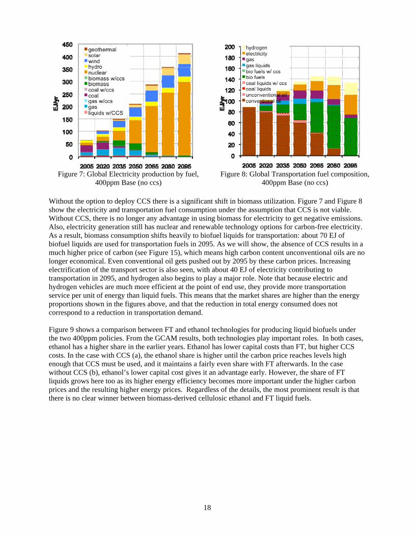
Figure 7: Global Electricity production by fuel, 400ppm Base (no ccs)

Figure 8: Global Transportation fuel composition, 400ppm Base (no ccs)

Without the option to deploy CCS there is a significant shift in biomass utilization. Figure 7 and Figure 8 show the electricity and transportation fuel consumption under the assumption that CCS is not viable. Without CCS, there is no longer any advantage in using biomass for electricity to get negative emissions. Also, electricity generation still has nuclear and renewable technology options for carbon-free electricity. As a result, biomass consumption shifts heavily to biofuel liquids for transportation: about 70 EJ of biofuel liquids are used for transportation fuels in 2095. As we will show, the absence of CCS results in a much higher price of carbon (see Figure 15), which means high carbon content unconventional oils are no longer economical. Even conventional oil gets pushed out by 2095 by these carbon prices. Increasing electrification of the transport sector is also seen, with about 40 EJ of electricity contributing to transportation in 2095, and hydrogen also begins to play a major role. Note that because electric and hydrogen vehicles are much more efficient at the point of end use, they provide more transportation service per unit of energy than liquid fuels. This means that the market shares are higher than the energy proportions shown in the figures above, and that the reduction in total energy consumed does not correspond to a reduction in transportation demand. Figure 9 shows a comparison between FT and ethanol technologies for producing liquid biofuels under the two 400ppm policies. From the GCAM results, both technologies play important roles. In both cases, ethanol has a higher share in the earlier years. Ethanol has lower capital costs than FT, but higher CCS costs. In the case with CCS (a), the ethanol share is higher until the carbon price reaches levels high enough that CCS must be used, and it maintains a fairly even share with FT afterwards. In the case without CCS (b), ethanol’s lower capital cost gives it an advantage early. However, the share of FT liquids grows here too as its higher energy efficiency becomes more important under the higher carbon prices and the resulting higher energy prices. Regardless of the details, the most prominent result is that there is no clear winner between biomass-derived cellulosic ethanol and FT liquid fuels.

19

(a) (b)

Figure 9: Global Biofuel production by technology, Base 400ppm scenario with CCS (a) and without

CCS (b) In Figures 10 through Figure 13, we summarize the biomass consumption results in terms of where the biomass is used in the energy system. We compare consumption results between the 400 ppm climate policy and the 450 ppm policy to highlight any impacts from a reduction in the stringency of the target. Comparing the results of Figure 10 to Figure 11, there is little clear difference in biomass use between these two climate targets when CCS is available. In the more stringent carbon policy case of 400 ppm, there is a more rapid expansion of biomass and a more rapid adoption of CCS. However, the pattern of use between electricity and refined liquids, as well as the overall scale, are very similar. This result reflects in part trade-offs between a higher value of biomass energy in the more stringent case but also a higher value on keeping land in forests to preserve and expand terrestrial carbon stocks. In Figure 12 and Figure 13, showing the 400 ppm and 450 ppm scenarios, respectively, we see that without the availability of CCS in any supply sector, the bulk of biomass use goes towards liquid fuels for transportation. Both cases show an even split between transportation and electricity use of biomass mid-century, but the high value of carbon at the end of the century leads to nearly all biomass being used in the transportation sector. Interestingly, the absence of CCS reduces the overall scale of biomass production and consumption considerably compared to the cases with CCS. Comparing these two figures, the total biomass in 2095 is actually lower in the 400 ppm case than for the 450 ppm case. This result shows that the higher carbon price in the 400 ppm case reduces the amount of land on which biomass production was economic compared to leaving it as forests. The effect is small here, but it highlights an important dynamic.

20

Figure 10: Biomass consumption by use, 400ppm Base

Figure 11: Biomass consumption by use, 450ppm Base

Figure 12: Biomass consumption by use, 400ppm Base (no ccs)

Figure 13: Biomass consumption by use, 450ppm Base (no ccs)

4.3 Carbon Emissions by Sector The changes in the electricity and transportation sector discussed in Section 4.2 drive changes in the overall system emissions, shown in Figure 14 for the 400ppm target, with and without CCS. With CCS available, emissions from the electricity sector grow through 2035 to meet rising demand, but then begin to rapidly decrease with the use of CCS with coal and natural gas, nuclear, and renewables. Eventually these zero or low-carbon technologies combine with widespread adoption of bioenergy with CCS, resulting in large negative emissions in the final years. Transportation sector emissions remain relatively flat, as conventional oil continues to play a major role in this sector. Transportation sector growth is largely met by lower emissions technologies, including electricity and biofuels with CCS. One way of interpreting these results is that the negative emissions from the electric sector offset the continued emissions from the transportation sector. As noted earlier without the availability of CCS, emissions must be cut at a much more rapid pace in order to get down to the 400 ppm target by the end of the century. Electric sector emissions grow only until 2020, then begin a slow but steady decline, approaching zero at the end of the century. After 2050, transportation sector emissions begin to decline as well, with the increasing adoption of biofuels along

21

with electricity and hydrogen. Without CCS, there are no negative emissions in the electric sector to offset emission from transportation. As a result, the transportation sector, as well as all other sectors, must reduce its emissions down to near zero by the end of the century. As seen in the next section, the difficulty of doing so is reflected in higher carbon prices.

(a) (b)

Figure 14: CO2 Emissions by sector, Base 400ppm (a) and Base 400ppm – no ccs (b)

4.4 Carbon Prices and Policy Costs

In each policy target and technology scenario, the GCAM model determines or solves for the equilibrium carbon price path to achieve the required emissions reductions. In GCAM, the price of carbon is set by the cost of reducing the last unit of emissions to meet the target. Figure 15 (a) compares the carbon price paths to meeting the scenarios studied here. The results show clearly that achieving CO2 concentration targets at the levels of stringency studied here would involve very high carbon prices, especially toward the end of the century. It is also clear that the availability of technologies, in this case CCS, would have a profound impact on the level of carbon prices required to hit a stringent target. From Figure 15 (a), the scenarios without CCS, the carbon prices must increase rapidly due to the more limited number of cost-effective options available for meeting the target. The scenarios with CCS see a substantial reduction in the carbon prices, for example, from about $300/mtC to $130/mtC under the 450ppm target and from about $700/mtC to $260/mtC under the 400ppm target. In all years, the availability of CCS brings the carbon prices to reach the 400ppm target comparable to the carbon prices for reaching the 450 target without CCS. While the carbon price is a reflection of the cost to reduce the last unit of emissions, GCAM also computes the total cost of reducing all the emissions from reference case levels to target levels. Figure 15 (b) shows global annual costs of the climate policies as computed by GCAM. Given the same technology assumptions, the 400ppm target has a much larger cost than the 450ppm cases, reflecting the added

22

difficulty in meeting this stringent target, not far removed from today’s conditions, rapidly approaching 390ppm (Tans 2009). Technologies can reduce these costs substantially, with the example studied here of the availability of CCS, along with the biomass and other low-carbon technologies included in the modeling analysis, cutting the 2095 costs in half. It should also be noted that without CCS available in the long term, costs are incurred more immediately as more reductions need to be made earlier in the century. For example, the 2035 cost for the 400 ppm scenario without CCS is three times more expensive than with CCS. With low CO2 concentration targets, biomass with CCS is clearly a very valuable tool.

(a) (b)

Figure 15: Carbon price, and the resulting policy cost for 400 ppm and 450ppm scenarios assuming differing technology portfolios

4.5 Biomass Production Compared to Other Studies The levels of biomass production shown in the results here, ranging from 120-160 EJ/per year in 2050 rising to 200-250 EJ/year, are large but comparable to several other integrated assessment models. The IMAGE model predicts 130-270 EJ can be produced at costs comparable to coal, and substantially more at higher prices (Hoogwijk et al. 2009). The MESSAGE model gives 100-200 EJ, and a MIT report predicts about 150 EJ for a 450ppm scenario (Obersteiner M 2002; Reilly et al. 2007). The IPCC Fourth Assessment report gives a wide range, 100-400 EJ, citing difficulty in obtaining accurate estimates because the use of dedicated energy crops depends on several factors, from food demands and nature protection to soil management and water reserves (Smith et al. 2007)

23

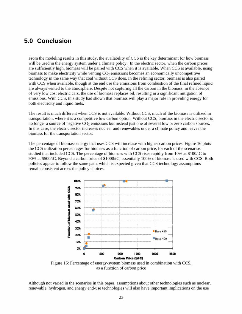
5.0 Conclusion From the modeling results in this study, the availability of CCS is the key determinant for how biomass will be used in the energy system under a climate policy. In the electric sector, when the carbon prices are sufficiently high, biomass will be paired with CCS when it is available. When CCS is available, using biomass to make electricity while venting CO2 emissions becomes an economically uncompetitive technology in the same way that coal without CCS does. In the refining sector, biomass is also paired with CCS when available, though at the end use the emissions from combustion of the final refined liquid are always vented to the atmosphere. Despite not capturing all the carbon in the biomass, in the absence of very low cost electric cars, the use of biomass replaces oil, resulting in a significant mitigation of emissions. With CCS, this study had shown that biomass will play a major role in providing energy for both electricity and liquid fuels. The result is much different when CCS is not available. Without CCS, much of the biomass is utilized in transportation, where it is a competitive low carbon option. Without CCS, biomass in the electric sector is no longer a source of negative CO2 emissions but instead just one of several low or zero carbon sources. In this case, the electric sector increases nuclear and renewables under a climate policy and leaves the biomass for the transportation sector. The percentage of biomass energy that uses CCS will increase with higher carbon prices. Figure 16 plots the CCS utilization percentages for biomass as a function of carbon price, for each of the scenarios studied that included CCS. The percentage of biomass with CCS rises rapidly from 10% at $100/tC to 90% at $500/tC. Beyond a carbon price of $1000/tC, essentially 100% of biomass is used with CCS. Both policies appear to follow the same path, which is expected given that CCS technology assumptions remain consistent across the policy choices.

Figure 16: Percentage of energy-system biomass used in combination with CCS,

as a function of carbon price Although not varied in the scenarios in this paper, assumptions about other technologies such as nuclear, renewable, hydrogen, and energy end-use technologies will also have important implications on the use

24

and value of biomass and biomass with CCS. For example, without new nuclear reactors and other low carbon alternatives, more biomass will be utilized in the electricity sector, in combination with an increased use of coal and gas with CCS. The availability of a high supply of low carbon electricity that nuclear and renewables provide is an important factor in allowing for biomass to be used in the transportation sector. Given a climate policy in which the carbon in land is valued equally with carbon in the energy system, biomass energy used in conjunction with CCS has the potential to be a major component of achieving low concentration targets. Despite the higher technology costs of CCS, the resulting negative emissions when used in conjunction with biomass are an important step to meeting strict carbon caps, and help to offset venting of CO2 from sectors of the energy system that may be more expensive to mitigate, such as oil use in transportation. The bottom line is that, either in the electricity or technology sector, biomass will be used with CCS when available. At the point of use, biomass is simply another fuel, differing very little from coal. In the presence of a strict emissions constraint, the high value place on CO2 means that the emissions from biomass are very valuable, and should be captured when feasible. While biomass alone is an attractive source of net-zero emission energy, when coupled with CCS, net negative emissions are far superior economically in a climate policy context.

25

References Aden, A., M. Ruth, K. Ibsen, J. Jechura, K. Neeves, J. Sheehan, B. Wallace, L. Montague, A. Slayton and

J. Lukas (2002). "Lignocellulosic Biomass to Ethanol Process Design and Economics Utilizing Co-Current Dilute Acid Prehydrolysis and Enzymatic Hydrolysis for Corn Stover." Other Information: PBD: 1 Jun 2002.

Brown, D., M. Gassner, T. Fuchino and F. MarÈchal (2009). "Thermo-economic analysis for the optimal conceptual design of biomass gasification energy conversion systems." Applied Thermal Engineering 29(11-12): 2137-2152.

Brown, R. A., N. J. Rosenberg, W. E. Easternling and C. J. Hays (1998). "Potential production of switchgrass and traditional crops under current and greehouse-altered climate in the 'MINK' region of the central United States." PNWD-2432, Pacific Northwest National Laboratory, Washington, D.C.

Calvin, K., J. Edmonds, B. Bond-Lamberty, L. Clarke, S. H. Kim, P. Kyle, S. J. Smith, A. Thomson and M. Wise (2009). "2.6: Limiting climate change to 450 ppm CO2 equivalent in the 21st century." Energy Economics In Press, Corrected Proof.

Chedid, R., M. Kobrosly and R. Ghajar (2007). "The potential of gas-to-liquid technology in the energy market: The case of Qatar." Energy Policy 35(10): 4799-4811.

Clarke, L., K. Calvin, J. Edmonds, P. Kyle and M. Wise (2009a). "When technology and climate policy meet: energy technology in an international policy context." Stavins R and J. Aldy (eds.) in Implementing Architectures for Agreement: Addressing Global Climate Change in the Post-Kyoto World. Cambridge University Press,

Clarke, L., P. Kyle, M. Wise, K. Calvin, J. Edmonds, S. Kim, M. Placet, and S. Smith. (2009b). CO2 Emissions Mitigation and Technological Advance: An Updated Analysis of Advanced Technology Scenarios, Pacific Northwest National Laboratory, Technical Report PNNL-18075.

Dooley, J. J. (2001). "The Need for a Biotechnology Revolution Focused on Energy and Climate Change."

Dooley, J. J. and R. T. Dahowski (2009). "Large-Scale U.S. Unconventional Fuels Production and the Role of Carbon Dioxide Capture and Storage Technologies in Reducing Their Greenhouse Gas Emissions." Energy Procedia 1(1): 4225-4232.

Edwards, R., J.-F. Larive, V. Mahieu and P. Rouveirolles (2006). "Well-to-wheels analysis of future automotive fuels and powertrains int he European context." WELL-TO-TANK report, Version 2b, May 2006. Available http://ies.jrc.ec.europa.eu/WTW,

Gregg, J. (2009). Spatial and Seasonal Distribution of Carbon Dioxide Emissions from Fossil-Fuel Combustion; Global, Regional, and National Potential for Sustainable Bioenergy from Residue Biomass and Municipal Solid Waste. Department of Geography. College Park, University of Maryland, College Park. PhD Dissertation.

Hamelinck, C. N., R. A. A. Suurs and A. P. C. Faaij (2005). "International bioenergy transport costs and energy balance." Biomass and Bioenergy 29(2): 114-134.

Hoogwijk, M., A. Faaij, B. de Vries and W. Turkenburg (2009). "Exploration of regional and global cost-supply curves of biomass energy from short-rotation crops at abandoned cropland and rest land under four IPCC SRES land-use scenarios." Biomass and Bioenergy 33(1): 26-43.

IPCC 2007a "Climate Change 2007: The Physical Science Basis. Contribution of Working Group I to the Fourth Assessment Report of the Intergovernmental Panel on Climate Change." [Solomon S, D. Qin, M. Manning, Z. Chen, M. Marquis, K.B. Averyt, M. Tignor and H. L. M. (eds.)] Cambridge University Press, Cambridge, United Kingdom and New York, NY, USA.

IPCC 2007b "Climate Change 2007: Mitigation. Contribution of Working Group III to the Fourth Assessment Report of the Intergovernmental Panel on Climate Change." [B. Metz, O.R. Davidson, P.R. Bosch, R. Dave and L. A. M. (eds.)] Cambridge University Press, Cambridge, United Kingdom and New York, NY, USA.

IPCC (2005). "IPCC special report on carbon dioxide capture and storage." B. [Metz, O. Davidson, H. d. Coninck, M. Loos and Meyer L (eds) Cambridge University Press for the Intergovernmental Panel on Climate Change, Cambridge.

26

Kim, S. H., J. A. Edmonds, J. Lurz, S. J. Smith and M. A. Wise (2006). "The ObjECTS: Framework for Integrated Assessment: Hybrid Modeling of Transportation." Journal Name: The Energy Journal, (Special Issue No. 2 2006):63.

Larson, E. D., G. Fiorese, G. Liu, R. H. Williams, T. G. Kreutz and S. Consonni (2009). "Co-production of synfuels and electricity from coal + biomass with zero net carbon emissions: An Illinois case study." Energy Procedia 1(1): 4371-4378.

Lindfeldt, E. G. and M. O. Westermark (2008). "System study of carbon dioxide (CO2) capture in bio-based motor fuel production." Energy 33(2): 352-361.

Matthews, H. D. and K. Caldeira (2007). "Transient climate–carbon simulations of planetary geoengineering." Proceedings of the National Academy of Sciences 104(24): 9949-9954.

McKendry, P. (2002). "Energy production from biomass (part 1): overview of biomass." Bioresource Technology 83(1): 37-46.

Obersteiner M, A. C., Moellersten K, Riahi K, Moreira J, Nilsson S, et al. (2002). "Biomass energy, carbon removal and permanent sequestration—a ‘Real Option’ for managing climate risk." IR-02-042, International Institute for Applied Systems Analysis, Laxenburg, Austria.

Paltsev, S., J. M. Reilly, H. D. Jacoby, A. C. Gurgel, G. E. Metcalf, A. P. Sokolov and J. F. Holak (2007). "Assessment of U.S. Cap-and-Trade Proposals." National Bureau of Economic Research Working Paper Series No. 13176.

Pannkuk, C. D. and P. R. Robichaud (2003). "Effectiveness of needle cast as reducing erosion after forest fires." Water Resources Research 39(12): 1333-1341.

Raupach, M. R., G. Marland, P. Ciais, C. Le Quere, J. G. Canadell, G. Klepper and C. B. Field (2007). "Global and regional drivers of accelerating CO2 emissions." Proceedings of the National Academy of Sciences 104(24): 10288-10293.

Reilly, J. M. and S. Paltsev (2007). Biomass Energy and Competition for Land. MIT Joint Program on the Science and Policy of Global Change, Report No. 147. Research Reports International (2009). "Utility Use of Biomass: 2nd Edition." October 2009. Evergreen,

Colorado. USA. Rhodes, J. and D. Keith (2008). "Biomass with capture: negative emissions within social and

environmental constraints: an editorial comment." Climatic Change 87(3): 321-328. Rosenberg, N. J. and J. Edmonds. (2005). "Climate change impacts for the conterminous USA an

integrated assessment." Smith, P., D. Martino, Z. Cai, H. Gwary, P. Janzen, B. Kumar, S. McCarl, S. Ogle, F. O'Mara, C. Rice, O.

Scholes and O. Sirotenko (2007). Agriculture in Climate Change 2007: Mitigation. Contribution of Working Group III to the Fourth Assessment Report of the Intergovernmental Panel on Climate Change [B. Metz, O.R. Davidson, P.R. Bosch, R. Dave, L.A. Meyer (eds)], Cambridge University Press, Cambridge, United Kingdom and New York, NY, USA. .

Tans, P. (2009). "Trends in Carbon Dioxide." NOAA/ESRL Retrieved August 10, 2009, from http://www.esrl.noaa.gov/gmd/ccgg/trends/.

US Climate Change Science Program (2007). "Scenarios of Greenhouse Gas Emissions and Atmospheric Concentrations." SAP 2.1a.

van Dyk, J. C., M. J. Keyser and M. Coertzen (2006). "Syngas production from South African coal sources using Sasol-Lurgi gasifiers." International Journal of Coal Geology 65(3-4): 243-253.

van Vliet, O. P. R., A. P. C. Faaij and W. C. Turkenburg (2009). "Fischer-Tropsch diesel production in a well-to-wheel perspective: A carbon, energy flow and cost analysis." Energy Conversion and Management 50(4): 855-876.

Williams, R. H., E. D. Larson, G. Liu and T. G. Kreutz (2009). "Fischer-Tropsch fuels from coal and biomass: Strategic advantages of once-through ("polygeneration") configurations." Energy Procedia 1(1): 4379-4386.

Wise, M., K. Calvin, A. Thomson, L. Clarke, B. Bond-Lamberty, R. Sands, S. J. Smith, A. Janetos and J. Edmonds (2009a). "Implications of Limiting CO2 Concentrations for Land Use and Energy." Science 324(5931): 1183-1186.

Wise, M., K. Calvin, A. Thomson, L. Clarke, B. Bond-Lamberty, R. Sands, S. J. Smith, A. Janetos and J. Edmonds (2009b). The Implications of Limiting CO2 Concentrations for Agriculture, Land Use,

27

Land-use Change Emissions and Bioenergy. Pacific Northwest National Laboratory, Technical Report PNNL-18341..

Wise, M., G. P. Kyle, J. J. Dooley and S. H. Kim (2010). "The impact of electric passenger transport technology under an economy-wide climate policy in the United States: Carbon dioxide emissions, coal use, and carbon dioxide capture and storage." International Journal of Greenhouse Gas Control In Press, Corrected Proof.

Wolf, A., A. Vidlund and E. Andersson (2006). "Energy-efficient pellet production in the forest industry--a study of obstacles and success factors." Biomass and Bioenergy 30(1): 38-45.