Biologically Plausible Error-drivenLearning using Local

Biologically Plausible Error-driven Learning using Local Activation Differences:The Generalized Recirculation Algorithm

Randall C. O’Reilly

Department of PsychologyCarnegie Mellon University

Pittsburgh, PA [email protected]

July 1, 1996

Neural Computation, 8:5, 895-938, 1996

Abstract

The error backpropagation learning algorithm (BP) is generally considered biologically implausible becauseit does not use locally available, activation-based variables. A version of BP that can be computed locallyusing bi-directional activation recirculation (Hinton & McClelland, 1988) instead of backpropagated errorderivatives is more biologically plausible. This paper presents a generalized version of the recirculation al-gorithm (GeneRec), which overcomes several limitations of the earlier algorithm by using a generic recur-rent network with sigmoidal units that can learn arbitrary input/output mappings. However, the contrastive-Hebbian learning algorithm (CHL, a.k.a. DBM or mean field learning) also uses local variables to performerror-driven learning in a sigmoidal recurrent network. CHL was derived in a stochastic framework (theBoltzmann machine), but has been extended to the deterministic case in various ways, all of which rely onproblematic approximations and assumptions, leading some to conclude that it is fundamentally flawed. Thispaper shows that CHL can be derived instead from within the BP framework via the GeneRec algorithm.CHL is a symmetry-preserving version of GeneRec which uses a simple approximation to the midpoint orsecond-order accurate Runge-Kutta method of numerical integration, which explains the generally fasterlearning speed of CHL compared to BP. Thus, all known fully general error-driven learning algorithms thatuse local activation-based variables in deterministic networks can be considered variations of the GeneRec al-gorithm (and indirectly, of the backpropagation algorithm). GeneRec therefore provides a promising frame-work for thinking about how the brain might perform error-driven learning. To further this goal, an explicitbiological mechanism is proposed which would be capable of implementing GeneRec-style learning. Thismechanism is consistent with available evidence regarding synaptic modification in neurons in the neocortexand hippocampus, and makes further predictions.

O’Reilly 1

Introduction

A long-standing objection to the error backpropagation learning algorithm (BP) (Rumelhart, Hinton, &Williams, 1986a) is that it is biologically implausible (Crick, 1989; Zipser & Andersen, 1988), principallybecause it requires error propagation to occur through a mechanism different from activation propagation.This makes the learning appear non-local, since the error terms are not locally available as a result of thepropagation of activation through the network. Several remedies for this problem have been suggested, butnone are fully satisfactory. One approach involves the use of an additional “error-network” whose job is tosend the error signals to the original network via an activation-based mechanism (Zipser & Rumelhart, 1990;Tesauro, 1990), but this merely replaces one kind of non-locality with another, activation-based kind of non-locality (and the problem of maintaining two sets of weights). Another approach uses a global reinforcementsignal instead of specific error signals (Mazzoni, Andersen, & Jordan, 1991), but this is not as powerful asstandard backpropagation.

The approach proposed by Hinton and McClelland (1988) is to use bi-directional activation recirculationwithin a single, recurrently connected network (with symmetric weights) to convey error signals. In orderto get this to work, they used a somewhat unwieldy four-stage activation update process that only works forauto-encoder networks. This paper presents a generalized version of the recirculation algorithm (GeneRec),which overcomes the limitations of the earlier algorithm by using a generic recurrent network with sigmoidalunits that can learn arbitrary input/output mappings. The GeneRec algorithm shows how a general form oferror backpropagation, which computes essentially the same error derivatives as the Almeida-Pineda (AP)algorithm (Almeida, 1987; Pineda, 1987b, 1987a, 1988) for recurrent networks under certain conditions, canbe performed in a biologically plausible fashion using only locally available activation variables.

GeneRec uses recurrent activation flow to communicate error signals from the output layer to the hid-den layer(s) via symmetric weights. This weight symmetry is an important condition for computing the cor-rect error derivatives. However, the “catch-22” is that GeneRec does not itself preserve the symmetry of theweights, and when it is modified so that it does, it no longer follows the same learning trajectory as AP, eventhough it is computing essentially the same error gradient. The empirical relationship between the derivativescomputed by GeneRec and AP backpropagation is explored in simulations reported in this paper.

The GeneRec algorithm has much in common with the contrastive Hebbian learning algorithm (CHL,a.k.a. the mean field or deterministic Boltzmann machine (DBM) learning algorithm), which also uses lo-cally available activation variables to perform error-driven learning in recurrently connected networks. Thisalgorithm was derived originally for stochastic networks whose activation states can be described by theBoltzmann distribution (Ackley, Hinton, & Sejnowski, 1985). In this context, CHL amounts to reducingthe distance between two probability distributions that arise in two phases of settling in the network. Thisalgorithm has been extended to the deterministic case through the use of approximations or restricted casesof the probabilistic one (Hinton, 1989b; Peterson & Anderson, 1987), and derived without the use of theBoltzmann distribution by using the continuous Hopfield energy function (Movellan, 1990). However, all ofthese derivations require problematic assumptions or approximations, leading some to conclude that CHL isfundamentally flawed for deterministic networks (Galland, 1993; Galland & Hinton, 1990).

It is shown in this paper that the CHL algorithm can be derived instead as a variant of the GeneRec algo-rithm, which establishes a more general formal relationship between the BP framework and the deterministicCHL rule than previous attempts (Peterson, 1991; Movellan, 1990; LeCun & Denker, 1991). This relation-ship means that all known fully general error-driven learning algorithms that use local activation-based vari-ables in deterministic networks can be considered variations of the GeneRec algorithm (and thus, indirectly,of the backpropagation algorithm as well). An important feature of the GeneRec-based derivation of CHL isthat the relationship between the learning properties of BP, GeneRec, and CHL can be more clearly under-stood. Another feature of this derivation is that it is completely general with respect to the activation function

2 The Generalized Recirculation Algorithm

used,� allowing CHL-like learning rules to be derived for many different cases.

CHL is equivalent to GeneRec when using a simple approximation to a second-order accurate numericalintegration technique known as the midpoint or second-order Runge-Kutta method, plus an additional sym-metry preservation constraint. The implementation of the midpoint method in GeneRec simply amounts tothe incorporation of the sending unit’s plus-phase activation state into the error derivative, and as such, itamounts to an on-line (per pattern) integration technique. This method results in faster learning by reducingthe amount of interference due to independently computed weight changes for a given pattern. This wouldexplain why CHL networks generally learn faster than otherwise equivalent BP networks (e.g., Peterson &Hartman, 1989; Movellan, 1990). A comparison of optimal learning speeds for all variants of GeneRec andfeedforward and AP recurrent backprop on four different problems is reported in this paper. The results ofthis comparison are consistent with the derived relationship between GeneRec and AP backpropagation, andwith the interpretation of CHL as a symmetric, midpoint version of GeneRec, and thus provide empiricalsupport for these theoretical claims.

The finding that CHL did not perform well at all in networks with multiple hidden layers (“deep” net-works), reported by Galland (1993), would appear to be problematic for the claim that CHL is performing afully general form of backpropagation, which can learn in deep networks. However, I was unable to repli-cate the Galland (1993) failure to learn the “family trees” problem (Hinton, 1986) using CHL. In simulationsreported below, I show that by simply increasing the number of hidden units (from 12 to 18), CHL networkscan learn the problem with 100% success rate, in a number of epochs on the same order as backpropagation.Thus, the existing simulation evidence seems to support the idea that CHL is performing a form of back-propagation, and not that it is a fundamentally flawed approximation to the Boltzmann machine as has beenargued (Galland, 1993; Galland & Hinton, 1990).

Given that the GeneRec family of algorithms encompasses all known ways of performing error-drivenlearning using locally-available activation variables, it provides a promising framework for thinking abouthow error-driven learning might be implemented in the brain. To further this goal, an explicit biologicalmechanism capable of implementing GeneRec-style learning is proposed. This mechanism is consistent withavailable evidence regarding synaptic modification in neurons in the neocortex and hippocampus, and makesfurther predictions.

Introduction to Algorithms and Notation

In addition to the original recirculation algorithm (Hinton & McClelland, 1988), the derivation of GeneRecdepends on ideas from several standard learning algorithms, including: feedforward error backpropagation(BP) (Rumelhart et al., 1986a) with the cross-entropy error term (Hinton, 1989a); the Almeida-Pineda (AP)algorithm for error backpropagation in a recurrent network (Almeida, 1987; Pineda, 1987b, 1987a, 1988);and the contrastive Hebbian learning algorithm (CHL) used in the Boltzmann machine and deterministicvariants (Ackley et al., 1985; Hinton, 1989b; Peterson & Anderson, 1987). The notation and equations forthese algorithms are summarized in this section, followed by a brief overview of the recirculation algorithmin the next section. This provides the basis for the development of the generalized recirculation algorithmpresented in subsequent sections.

Feedforward Error Backpropagation

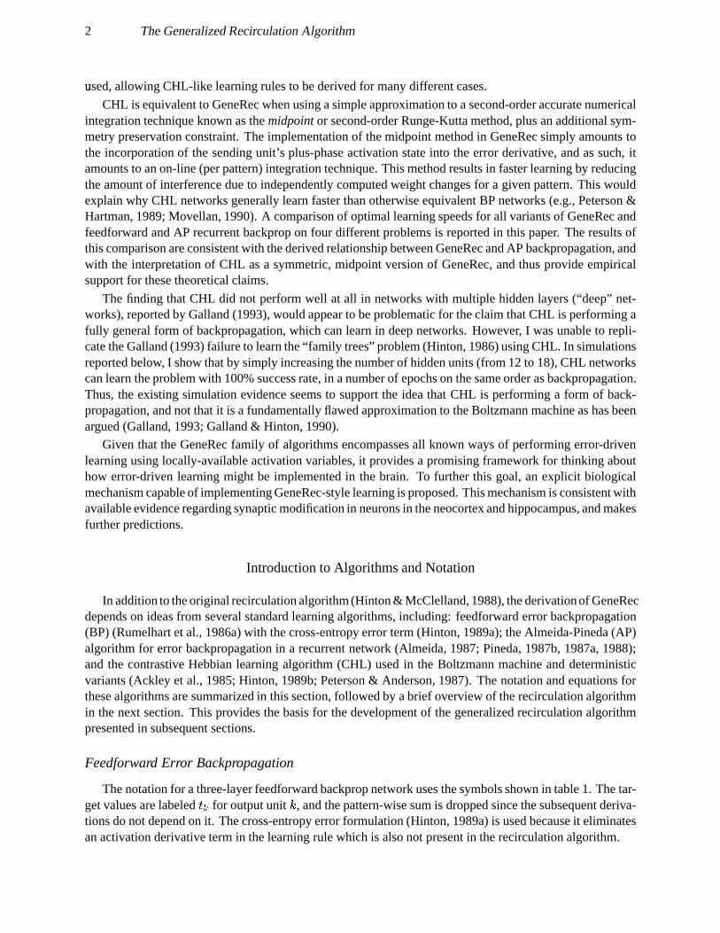
The notation for a three-layer feedforward backprop network uses the symbols shown in table 1. The tar-get values are labeled

��for output unit � , and the pattern-wise sum is dropped since the subsequent deriva-

tions do not depend on it. The cross-entropy error formulation (Hinton, 1989a) is used because it eliminatesan activation derivative term in the learning rule which is also not present in the recirculation algorithm.

O’Reilly 3

Layer (index) Net Input Activation

Input ( � ) — �� stimulus inputHidden ( ) � �� Output ( � ) � � ��

Table 1: Variables in a 3 layer backprop network. ��! #" is the standard sigmoidal activation function ��$ "&%�')(*��',+-�.0/ " .The cross-entropy error is defined as:1 ��2 � � �436587 � �:9 �);:< � � � 3=5>7 �);:<?� � � (1)

and the derivative of1

with respect to a weight into an output unit is:@ 1@ � � � � A 1A � � A � �A � �@ � �@ � � �� B �� < �C;D< �� );E<F� � �CG �4HI�� <F� � �� (2)

where � H �J� � � is the first derivative of the sigmoidal activation function with respect to the net input: � � �);:<� � � , which is canceled by the denominator of the error term. In order to train the weights into the hiddenunits, the impact a given hidden unit has on the error term needs to be determined:@ 1@ � � 2 � A 1A � � A � �A � �

@ � �@ �� < 2 � � �K� <F� � � � � � (3)

which can then be used to take the derivative of the error function with respect to the input to hidden unitweights: @ 1@ � � � � @ 1@ � A ��A � �

@ � �@ � � �� < 2 � � �� <?� � � � � � � H �� (4)

which provides the basis for adapting the weights.

Almeida-Pineda Recurrent Backpropagation

The AP version of backpropagation is essentially the same as the feedforward one described above exceptthat it allows for the network to have recurrent (bidirectional) connectivity. Thus, the network is trained tosettle into a stable activation state with the output units in the target state, based on a given input patternclamped over the input units. This is the version of BP that the GeneRec algorithm, which also uses recurrentconnectivity, approximates most closely. The same basic notation and cross-entropy error term as describedfor feedforward BP are used to describe the AP algorithm, except that the net input terms ( � ) can now includeinput from any other unit in the network, not only those in lower layers.


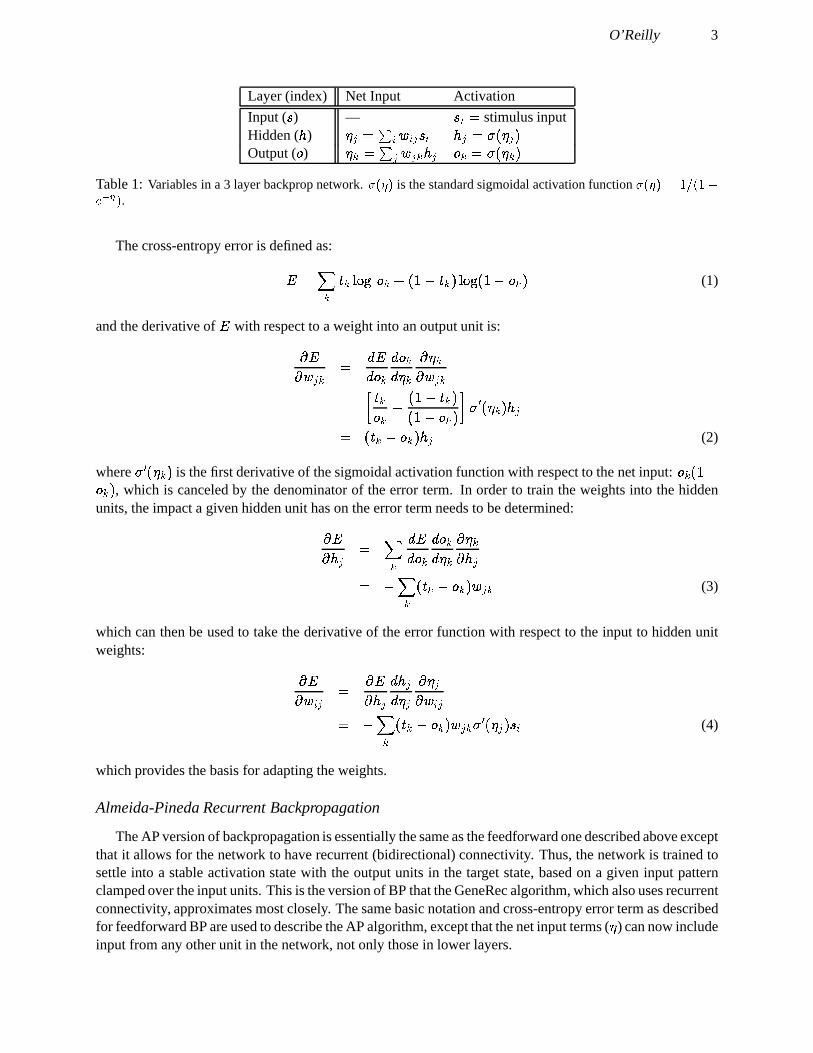
Layer Phase Net Input Activation

Input ( � ) — — �� stimulus inputHidden ( ) - �4L� � � � � � � �� 9 � � � � � �>L� 4L� ��4L� �

+ �NM� �� 9 � � � � �� M� NM� ��NM� �Output ( � ) - � L� �� L� � L� �� L� �

+ — � M� � � �Table 2: Equilibrium network variables in a three layer network having reciprocal connectivity between the hiddenand output layers with symmetric weights ( O4P)QR%?O&QJP ), and phases over the output units such that the target is clampedin the plus phase, and not in the minus phase. ��$ " is the standard sigmoidal activation function.

The activation states in AP are updated according to a discrete-time approximation of the following dif-ferential equation, which is integrated over time with respect to the net input terms S :

A � �A � �T<:� � 9 2 � � � � ��8�!� (5)

This equation can be iteratively applied until the network settles into a stable equilibrium state (i.e., until thechange in activation state goes below a small threshold value), which it will provably do if the weights aresymmetric (Hopfield, 1984), and often even if they are not (Galland & Hinton, 1991).

In the same way that the activations are iteratively updated to allow for recurrent activation dynamics,the error propagation in the AP algorithm is also performed iteratively. The iterative error propagation in APoperates on a new variable U � which represents the current estimate of the derivative of the error with respectto the net input to the unit, V�WV�XKY . This variable is updated according to:

A U �A � �T<:U � 9 � H �J� � � 2 � � � � U � 9[Z � (6)

whereZ � is the externally “injected” error for output units with target activations. This equation is iteratively

applied until the U � variables settle into an equilibrium state (i.e., until the change in U � falls below a smallthreshold value). The weights are then adjusted as in feedforward BP (4), with U � providing the V�WV�XKY term.

Contrastive Hebbian Learning

The contrastive-Hebbian learning algorithm (CHL) used in the stochastic Boltzmann machine and deter-ministic variants is based on the differences between activation states in two different phases. As in the APalgorithm, the connectivity is recurrent, and activation states (in the deterministic version) can be computedaccording to (5). As will be discussed below, the use of locally-computable activation differences instead ofthe non-local error backpropagation used in the BP and AP algorithms is more biologically plausible. TheGeneRec algorithm, from which the CHL algorithm can be derived as a special case, uses the same notionof activation phases.

The two phases of activation states used in CHL are the plus phase states, which result from both inputand target being presented to the network, and provide a training signal when compared to the minus phaseactivations, which result from just the input pattern being presented. The equilibrium network variables (i.e.,the states after the iterative updating procedure of (5) has been applied) for each phase in such a system arelabeled as in table 2.\

It is also possible to incrementally update the activations instead of the net inputs, but this limits the ability of units to changetheir state rapidly, since the largest activation value is 1, while net inputs are not bounded.

O’Reilly 5

The CHL learning rule for deterministic recurrent networks can be expressed in terms of generic activa-tion states ] (which can be from any layer in the network) as follows:;^`_ � � �a�b��]cM� ]cM� �,<[��] L� ] L� � (7)

where ]>� is the sending unit and ] � is the receiving unit. Thus, CHL is simply the difference between the preand post-synaptic activation coproducts in the plus and minus phases. Each coproduct term is equivalent tothe derivative of the energy or “harmony” function for the network with respect to the weight:1 � 2 � 2 � ] � ]8� � � � (8)

and the intuitive interpretation of this rule is that it decreases the energy or increases the harmony of the plus-phase state and vice-versa for the minus-phase state (see Ackley et al., 1985; Peterson & Anderson, 1987;Hinton, 1989b; Movellan, 1990, for details).

The Recirculation Algorithm

The original Hinton and McClelland (1988) recirculation algorithm is based on the feedforward BP algo-rithm. The GeneRec algorithm, which is more closely related to the AP recurrent version of backpropagation,borrows two key insights from the recirculation algorithm. These insights provide a means of overcomingthe main problem with the standard backprop formulation from a neural plausibility standpoint, which is themanner in which a hidden unit computes its own error contribution. This is shown in (3). The problem is thatthe hidden unit is required to access the computed quantity ( V�WVedKf ), which depends on variables at the outputunit only. This is the crux of the non-locality of error information in backpropagation.

The first key insight that can be extracted from the recirculation algorithm is that (3) can be expressed asthe difference between two terms, each of which look much like a net-input to the hidden unit:@ 1@ �� T<hg 2 � �� < 2 � � � � � ��i (9)

Thus, instead of having a separate error-backpropagation phase to communicate error signals, one can thinkin terms of standard activation propagation occurring via reciprocal (and symmetric) weights that come fromthe output units to the hidden units. The error contribution for the hidden unit can then be expressed in termsof the difference between two net-input terms. One net-input term is just that which would be received whenthe output units had the target activations

�K�clamped on them, and the other is that which would be received

when the outputs have their feed-forward activation values � � .In order to take advantage of a net-input based error signal, Hinton and McClelland (1988) used an auto-

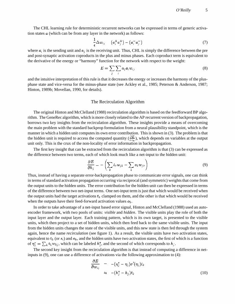
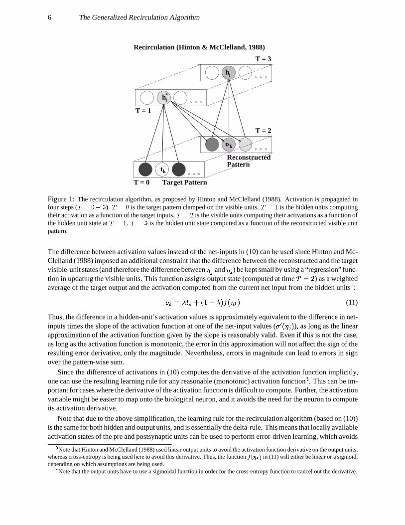
encoder framework, with two pools of units: visible and hidden. The visible units play the role of both theinput layer and the output layer. Each training pattern, which is its own target, is presented to the visibleunits, which then project to a set of hidden units, which then feed back to the same visible units. The inputfrom the hidden units changes the state of the visible units, and this new state is then fed through the systemagain, hence the name recirculation (see figure 1). As a result, the visible units have two activation states,equivalent to

��(or �� ) and � � , and the hidden units have two activation states, the first of which is a function

of �Nj� �� , which can be labeled �j� , and the second of which corresponds to c� .The second key insight from the recirculation algorithm is that instead of computing a difference in net-

inputs in (9), one can use a difference of activations via the following approximation to (4):@ 1@ � � � � <a�� j� <k� � ��4HI�� l <a�� j� <F � � �� (10)


tk

T = 0

T = 1

hj*

T = 3

T = 2

ko

hj

Target Pattern

ReconstructedPattern

Recirculation (Hinton & McClelland, 1988)

Figure 1: The recirculation algorithm, as proposed by Hinton and McClelland (1988). Activation is propagated infour steps ( mF%?nRoqp ). mr%sn is the target pattern clamped on the visible units. mF%t' is the hidden units computingtheir activation as a function of the target inputs. mF%Fu is the visible units computing their activations as a function ofthe hidden unit state at mF%�' . ms%?p is the hidden unit state computed as a function of the reconstructed visible unitpattern.

The difference between activation values instead of the net-inputs in (10) can be used since Hinton and Mc-Clelland (1988) imposed an additional constraint that the difference between the reconstructed and the targetvisible-unit states (and therefore the difference between �Nj� and � � ) be kept small by using a “regression” func-tion in updating the visible units. This function assigns output state (computed at time v��w ) as a weightedaverage of the target output and the activation computed from the current net input from the hidden units x :� � �zy �K� 9 �);:<[y4��{|�� (11)

Thus, the difference in a hidden-unit’s activation values is approximately equivalent to the difference in net-inputs times the slope of the activation function at one of the net-input values ( � H �� ), as long as the linearapproximation of the activation function given by the slope is reasonably valid. Even if this is not the case,as long as the activation function is monotonic, the error in this approximation will not affect the sign of theresulting error derivative, only the magnitude. Nevertheless, errors in magnitude can lead to errors in signover the pattern-wise sum.

Since the difference of activations in (10) computes the derivative of the activation function implicitly,one can use the resulting learning rule for any reasonable (monotonic) activation function } . This can be im-portant for cases where the derivative of the activation function is difficult to compute. Further, the activationvariable might be easier to map onto the biological neuron, and it avoids the need for the neuron to computeits activation derivative.

Note that due to the above simplification, the learning rule for the recirculation algorithm (based on (10))is the same for both hidden and output units, and is essentially the delta-rule. This means that locally availableactivation states of the pre and postsynaptic units can be used to perform error-driven learning, which avoids~

Note that Hinton and McClelland (1988) used linear output units to avoid the activation function derivative on the output units,whereas cross-entropy is being used here to avoid this derivative. Thus, the function �c�� f)� in (11) will either be linear or a sigmoid,depending on which assumptions are being used.�

Note that the output units have to use a sigmoidal function in order for the cross-entropy function to cancel out the derivative.

O’Reilly 7

the�

need for a biologically troublesome error backpropagation mechanism that is different from the normalpropagation of activation through the network.

Phase-Based Learning and Generalized Recirculation

While the recirculation algorithm is more biologically plausible than standard feedforward error back-propagation, it is limited to learning auto-encoder problems. Further, the recirculation activation propagationsequence requires a detailed level of control over the flow of activation through the network and its interac-tion with learning. However, the critical insights about computing error signals using differences in net input(or activation) terms can be applied to the more general case of a standard three-layer network for learning in-put to output mappings. This section presents such a generalized recirculation or GeneRec algorithm, whichuses standard recurrent activation dynamics (as used in the AP and CHL algorithms) to communicate errorsignals instead of the recirculation technique. Instead of using the four stages of activations used in recir-culation, GeneRec uses two activation phases as in the CHL algorithm described above. Thus, in terms ofactivation states, GeneRec is identical to the deterministic CHL algorithm, and the same notation is used todescribe it.

The learning rule for GeneRec is simply the application of the two key insights from the recirculationalgorithm to the AP recurrent backpropagation algorithm instead of the feedforward BP algorithm, whichwas the basis of the recirculation algorithm. If the recurrent connections between the hidden and output unitsare ignored so that the error on the output layer is held constant, it is easy to show that the fixed point solutionto the iterative AP error updating equation (6) (i.e., where �K� Y�K� �� for hidden unit error U�� ) is of the sameform as feedforward backpropagation. This means that the same recirculation trick of computing the errorsignal as a difference of net input (or activation) terms can be used:U`�� H �� 2 � � � � U`��l � H �� g 2 � � � � � �K� <F� � � il �4HI�� gc2 � � � � � � <F2 � � � �� i (12)

Thus, assuming constant error on the output layer, the equilibrium error gradient computed for hidden unitsin AP is equivalent to the difference between the GeneRec equilibrium net input states in the plus and minusphases. Note that the minus phase activations in GeneRec are identical to the AP activation states. The dif-ference of activation states can be substituted for net input differences times the derivative of the activationfunction by the approximation introduced in recirculation, resulting in the following equilibrium unit errorgradient: U �� l �M� <? L� (13)

Note that while the hidden unit states in GeneRec also reflect the constant net input from the input layer(in addition to the output-layer activations that communicate the necessary error gradient information), thiscancels out in the difference computation of (13). However, this constant input to the hidden units from theinput layer in both phases can play the role of the regression update equation (11) in recirculation. To theextent that this input is reasonably large and it biases the hidden units towards one end of the sigmoid or theother, this bias will tend to moderate the differences between L� and M� , making their difference a reasonableapproximation to the differences of their respective net inputs times the slope of the activation function.


While the analysis presented above is useful for seeing how GeneRec equilibrium activation states couldapproximate the equilibrium error gradient computed by AP, the AP algorithm actually performs iterativeupdating of the error variable ( U � ). Thus, it would have to be the case that iterative updating of this singlevariable is equivalent to the iterative updating of each of the activation states (plus and minus) in GeneRec,and then taking the difference. This relationship can be expressed by writing GeneRec in the AP notation.First, we define two components to the error variable U � , which are effectively the same as the GeneRec plusand minus phase net inputs (ignoring the net input from the input units, which is subtracted out in the endanyway): A U M�A � � <:U`M� 9 2 � � � � � � (14)

A U L�A � � <:U L� 9 2 � � � � �� (15)

Then, we approximate the fixed point of U � with the difference of the fixed points of these two variables:U`�� l � H �� U � M� <kU � L� �l �M� <F L� (16)

which can be approximated by the subtraction of the GeneRec equilibrium activation states as discussed pre-viously.

Unfortunately, the validity of this approximation is not guaranteed by any proof that this author is awareof. However, there are several properties of the equations that lend some credibility to it. First, the part that isa function of

�K�on the output units, U M� , is effectively a constant, and the other part, U L� , is just the activation

updating procedure that both GeneRec and AP have in common. Further, given that the fixed point solu-tions of the GeneRec and AP equations are the same when recurrent influences are ignored, and the patternof recurrent influences is given by the same set of weights, it is likely that the additional effects of recurrencewill be in the same direction for both GeneRec and AP. However, short of a proof, these arguments requiresubstantiation from simulation results comparing the differences between the error derivatives computed byGeneRec and AP. The results presented later in the paper confirm that GeneRec computes essentially thesame error derivatives as AP in a three layer network (as long as the weights are symmetric). This approxi-mation deteriorates only slightly in networks with multiple hidden layers, where the effects of recurrence areconsiderably greater.

As in the recirculation algorithm, it is important for the above approximation that the weights into thehidden units from the output units have the same values as the corresponding weights that the output unitsreceive from the hidden units. This is the familiar symmetric weight constraint, which is also necessary toprove that a network will settle into a stable equilibrium (Hopfield, 1984). We will revisit this constraintseveral times during the paper. However, for the time being, we will assume that the weights are symmetric.

Finally, virtually all deterministic recurrent networks including GeneRec suffer from the problem thatchanges in weights based on gradient information computed on equilibrium activations might not result inthe network settling into an activation state with lower error the next time around. This is due to the factthat small weight changes can affect the settling trajectory in unpredictable ways, resulting in an entirely dif-ferent equilibrium activation state than the one settled into last time. While it is important to keep in mindthe possibility of discontinuities in the progression of activation states over learning, there is some basis foroptimism on this issue. For example, in his justification of the deterministic version of the Boltzmann ma-chine (DBM) Hinton (1989b) supplies several arguments (which are substantiated by a number of empiricalfindings) justifying the assumption that small weight changes will generally lead to a contiguous equilibriumstate of unit activities in a recurrent network.

O’Reilly 9

To summarize, the learning rule for GeneRec that computes the error backpropagation gradient locallyvia recurrent activation propagation is the same as that for recirculation, having the form of the delta-rule. Itcan be stated as follows in terms of a sending unit with activation ]>� and a receiving unit with activation ] � :;^ _ � � � ��] L� ��] M� <s] L� � (17)

As shown above, this learning rule will compute the same error derivatives as the AP recurrent backpropa-gation procedure under the following conditions:� Iterative updating of the error term ( U � ) can be approximated by the separate iterative updating of the

two activation terms ( �M� and L� ) and then taking their difference.� The reciprocal weights are symmetric ( � � � � � � � ).� Differences in net inputs times the activation function derivative can be approximated by differencesin the activation values.

The Relationship Between GeneRec and CHL

The GeneRec learning rule given by (17) and the CHL learning rule given by (7) are both simple expres-sions that involve a difference between plus and minus phase activations. This raises the possibility that theycould somehow be related to each other. Indeed, as described below, there are two different ways in whichGeneRec can be modified that, when combined, yield (7).

The GeneRec learning rule can be divided into two parts, one of which represents the derivative of theerror with respect to the unit (the difference of that unit’s plus and minus activations, ]cM� <�] L� ), and the otherwhich represents the contribution of a particular weight to this error term (the sending unit’s activation, ] L� ).It is the phase of this latter term which is the source of the first modification. In standard feedforward or APrecurrent backpropagation, there is only one activation term associated with each unit, which is equivalentto the minus-phase activation in the GeneRec phase-based framework. Thus, the contribution of the sendingunit is naturally evaluated with respect to this activation, and that is why ] L� appears in the GeneRec learningrule.

However, given that GeneRec has another activation term corresponding to the plus-phase state of theunits, one might wonder if the derivative of the weight should be evaluated with respect to this activationinstead. After all, the plus phase activation value will likely be a more accurate reflection of the eventualcontribution of a given unit after other weights in the network are updated. In some sense, this value antic-ipates the weight changes that will lead to having the correct target values activated, and learning based onit might avoid some interference.

On the other hand, the minus phase activation reflects the actual contribution of the sending unit to thecurrent error signal, and it seems reasonable that credit assignment should be based on it. Given that thereare arguments in favor of both phases, one approach would be to simply use the average of both of them.Doing this results in the following weight update rule:;^`_ � � �� ;w ��] L� 9 ]0M� ��]0M� <F] L� � (18)

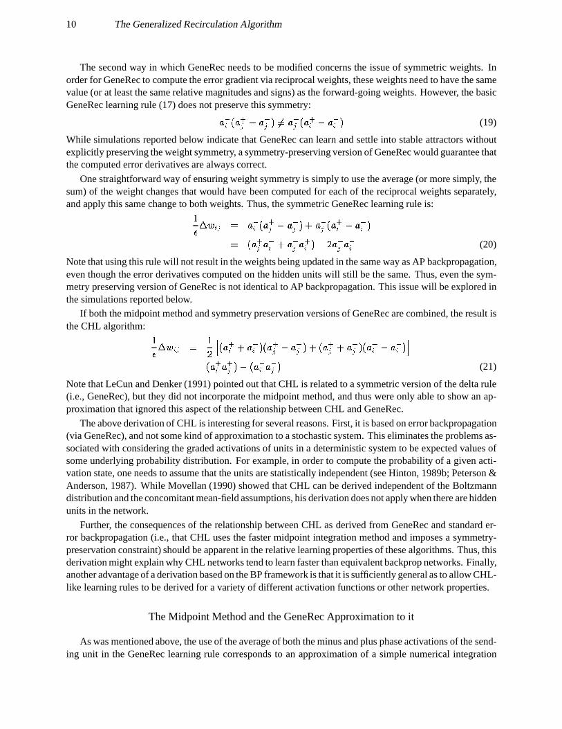
This is the first way in which GeneRec needs to be modified to make it equivalent to CHL. As will be dis-cussed in detail below, this modification of GeneRec corresponds to a simple approximation of the midpointor second-order accurate Runge-Kutta integration technique. The consequences of the midpoint method forlearning speed will be explored in the simulations reported below.


The second way in which GeneRec needs to be modified concerns the issue of symmetric weights. Inorder for GeneRec to compute the error gradient via reciprocal weights, these weights need to have the samevalue (or at least the same relative magnitudes and signs) as the forward-going weights. However, the basicGeneRec learning rule (17) does not preserve this symmetry:] L� ��]cM� <F] L� �D��] L� ��]0M� <?] L� � (19)

While simulations reported below indicate that GeneRec can learn and settle into stable attractors withoutexplicitly preserving the weight symmetry, a symmetry-preserving version of GeneRec would guarantee thatthe computed error derivatives are always correct.

One straightforward way of ensuring weight symmetry is simply to use the average (or more simply, thesum) of the weight changes that would have been computed for each of the reciprocal weights separately,and apply this same change to both weights. Thus, the symmetric GeneRec learning rule is:;^ _ � � � � ] L� ��]cM� <s] L� � 9 ] L� ��]cM� <F] L� �� ] M� ] L� 9 ] L� ] M� ��<Fw8] L� ] L� (20)

Note that using this rule will not result in the weights being updated in the same way as AP backpropagation,even though the error derivatives computed on the hidden units will still be the same. Thus, even the sym-metry preserving version of GeneRec is not identical to AP backpropagation. This issue will be explored inthe simulations reported below.

If both the midpoint method and symmetry preservation versions of GeneRec are combined, the result isthe CHL algorithm: ;^N_ � � � � ;wF� ��]cM� 9 ] L� ��]cM� <F] L� � 9 ��]cM� 9 ] L� ��]cM� <?] L� �� ]0M� ]cM� ��<��] L� ] L� � (21)

Note that LeCun and Denker (1991) pointed out that CHL is related to a symmetric version of the delta rule(i.e., GeneRec), but they did not incorporate the midpoint method, and thus were only able to show an ap-proximation that ignored this aspect of the relationship between CHL and GeneRec.

The above derivation of CHL is interesting for several reasons. First, it is based on error backpropagation(via GeneRec), and not some kind of approximation to a stochastic system. This eliminates the problems as-sociated with considering the graded activations of units in a deterministic system to be expected values ofsome underlying probability distribution. For example, in order to compute the probability of a given acti-vation state, one needs to assume that the units are statistically independent (see Hinton, 1989b; Peterson &Anderson, 1987). While Movellan (1990) showed that CHL can be derived independent of the Boltzmanndistribution and the concomitant mean-field assumptions, his derivation does not apply when there are hiddenunits in the network.

Further, the consequences of the relationship between CHL as derived from GeneRec and standard er-ror backpropagation (i.e., that CHL uses the faster midpoint integration method and imposes a symmetry-preservation constraint) should be apparent in the relative learning properties of these algorithms. Thus, thisderivation might explain why CHL networks tend to learn faster than equivalent backprop networks. Finally,another advantage of a derivation based on the BP framework is that it is sufficiently general as to allow CHL-like learning rules to be derived for a variety of different activation functions or other network properties.

The Midpoint Method and the GeneRec Approximation to it

As was mentioned above, the use of the average of both the minus and plus phase activations of the send-ing unit in the GeneRec learning rule corresponds to an approximation of a simple numerical integration

O’Reilly 11

f’( )y1

t1

t t2 3

y1

y2 y3

y*

midpoint

2

y1 y*+2

2

trial step

y1

actual step

2

y1 y*+2

2f’( )

+ y1 y*+2

2f’( )

f(y)

4

3

1 5

Figure 2: The midpoint method. At each point, a trial step is taken along the derivative at that point, and the derivativere-computed at the midpoint between the point and the trial step. This derivative is then used to take the actual step tothe next point, and so on.

technique for differential equations known as the midpoint or second-order accurate Runge-Kutta method(Press, Flannery, Teukolsky, & Vetterling, 1988).

The midpoint method attains second-order accuracy without the explicit computation of second deriva-tives by evaluating the first derivatives twice and combining the results so as to minimize the integrationerror. It can be illustrated with the following simple differential equation:

A UN� � �A � ��{�H��UN� � �� (22)

The simplest way in which the value of the variable U can be integrated is by using a difference equationapproximation to the continuous differential equation:U � M S ��U � 9 ^ {�H!��U � � 9�� ^ x � (23)

with a step size of^, and an accuracy to first order in the Taylor series expansion of {|��U � � (and thus an error

term of order^ x ). This integration technique is known as the forward Euler method, and is commonly used in

neural network gradient descent algorithms such as BP. By comparison with (23), the midpoint method takesa “trial” step using the forward Euler method, resulting in an estimate of the next function value (denoted bythe *): U j� M S ��U � 9 ^ { H ��U � � (24)

This estimate is then used to compute the actual step, which is the derivative computed at a point halfwaybetween the current U � and estimated U j� M S values (see figure 2):

U � M S ��U � 9 ^ {�H,� U � 9 U j� M Sw � 9?� � ^ } � (25)

In terms of a Taylor series expansion of the function {|��U � � at the point U � , evaluating the derivative at themidpoint as in (25) cancels out the first-order error term (

� � ^ x � ), resulting in a method with second-order


accuracy� (Press et al., 1988). Intuitively, the midpoint method is able to “anticipate” the curvature of thegradient, and avoid going off too far in the wrong direction.

There are a number of ways the midpoint method could be applied to error backpropagation. Perhaps themost “correct” way of doing it would be to run an entire batch of training patterns to compute the trial stepweight derivative, and then run another batch of patterns with the weights half way between their current andthe trial step values to get the actual weight changes to be made. However, this would require roughly twicethe number of computations per weight update as standard batch-mode backpropagation, and the two passesof batch-mode learning is not particularly biologically plausible.

The GeneRec version of the midpoint method as given by (18) is an approximation to the “correct” versionin two respects:

1. The plus-phase activation value is used as an on-line estimate of the activations that would result froma forward Euler step over the weights. This estimate has the advantages of being available withoutany additional computation, and it can be used with on-line weight updating, solving both of the majorproblems with the “correct” version. The relationship between the plus-phase activation and a forwardEuler step along the error gradient makes sense given that the plus-phase activation is the “target” state,which is therefore in the direction of reducing the error. Appendix A gives a more formal analysis ofthis relationship. This analysis shows that the plus phase activation, which does not depend on thelearning rate parameter, typically over-estimates the size of a trial Euler step. Thus, the use of theplus-phase activation means that the precise midpoint is not actually being computed. Nevertheless,the anticipatory function of this method is still served when the trial step is exaggerated. Indeed, thesimulation results described below indicate that it can actually be advantageous in certain tasks to takea larger trial step.

2. The midpoint method is applied only to the portion of the derivative that distributes the unit’s errorterm amongst its incoming weights, and not to the computation of the error term itself. Thus, the errorterm ��]0M� <[] L� � from (18) is the same as in the standard forward Euler integration method, and onlythe sending activations are evaluated at the midpoint between the current and the trial step: Sx �K] L� 9]0M� � . This selective application of the midpoint method is particularly efficient for the case of on-linebackpropagation because a midpoint value of the unit error term, especially on a single-pattern basis,will typically be smaller than the original error value, since the trial step is in the direction of reducingerror. Thus, using the midpoint error value would actually slow learning by reducing the effectivelearning rate.

To summarize, the advantage of using the approximate midpoint method represented by (18) is that it is sosimple to compute, and it appears to reliably speed up learning while still using on-line learning. While othermore sophisticated integration techniques have been developed for batch-mode BP (see Battiti, 1992 for areview), they typically require considerable additional computation per step, and are not very biologicallyplausible.

The GeneRec Approximate Midpoint Method in Backpropagation

In order to validate the idea that CHL is equivalent to GeneRec using the approximation to the midpointmethod described above, this approximation can be implemented in a standard backpropagation network andthe relative learning speed advantage of this method compared for the two different algorithms. If similarkinds of speedups are found in both GeneRec and backpropagation, this would support the derivation of CHLas given in this paper. Such comparisons are described in the following simulation section.

There are two versions of the GeneRec approximate midpoint method that are relevant to consider. Oneis a weight-based method which computes the sending unit’s trial step activation ( j� ) based on the trial step

O’Reilly 13

weights,� and the other is a simpler approximation which uses the unit’s error derivative to estimate the trialstep activation. In both cases, the resulting trial step activation state j� is averaged with the current activationvalue � to obtain a midpoint activation value which is used as the sending activation state for backpropaga-tion weight updating: ;^ _ � � � � ;w �� j� 9 � �� <?� � � (26)

This corresponds to the GeneRec version of the midpoint method as given in (18). Note that in a three-layernetwork, only the hidden-to-output weights are affected, since there is no trial step activation value for theinput units.

In the BP weight-based midpoint approximation, the trial step activation is computed as if the weightshad been updated by the trial step weight error derivatives as follows:

� j� � 2 � � � g � � � 9 ^ �� < @ 1@ � � � i j� � �� j� � (27)

where^ �� is a learning-rate-like constant that determines the size of the trial step taken. Note that, in keeping

with the GeneRec approximation, the actual learning rate^

is not included in this equation. Thus, dependingon the relative sizes of

^ �� and^, the estimated trial step activation given by (27) can over-estimate the size

of an actual trial step activation. In order to evaluate the effects of this over-estimation, a range of^ �� values

are explored.

The BP unit-error-based method uses the fact that each weight will be changed in proportion to the deriva-tive of the error with respect to the unit’s net input, V�WV�XKY , to avoid the additional traversal of the weights:

� j� � � � 9 ^ �� < @ 1@ � � j� � �� j� � (28)

where � is the number of receiving weights (fan-in). In this case, the trial step size parameter^ �� also re-

flects the average activity level over the input layer, since each input weight would actually be changed byan amount proportional to the activity of the sending unit. The comments regarding

^ �� above also apply tothis case.

Note that it is the unit-error-based version of the midpoint method that most closely corresponds to theversion used in CHL, since both are based on the error derivative with respect to the unit, not the weights intothe unit. As the simulations reported below indicate, the midpoint method can speed up on-line BP learningby nearly a factor of two. Further, the unit-error-based version is quite simple and requires little extra compu-tation to implement. Finally, while the unit-error-based version could be applied directly to Almeida-Pinedabackpropagation, the same is not true for the weight-based version, which would require an additional acti-vation settling based on the trial step weights. Thus, in order to compare these two ways of implementingthe approximate midpoint method, the results presented below are for feedforward backprop networks.

Simulation Experiments

The first set of simulations reported in this section is a comparison of the learning speed between sev-eral varieties of GeneRec (including symmetric, midpoint, and CHL) and BP with and without the midpointintegration method. This gives a general sense of the comparative learning properties of the different al-gorithms, and provides empirical evidence in support of the predicted relationships amongst the algorithms


investigated.

In the second set of simulations, a detailed comparison of the weight derivatives computed bythe Almeida-Pineda version of backpropagation and GeneRec is performed, showing that they both computethe same error derivatives under certain conditions.

Learning Speed Comparisons

While it is notoriously difficult to perform useful comparisons between different learning algorithms, suchcomparisons could provide some empirical evidence necessary for evaluating the theoretical claims madeabove in the derivation of the GeneRec algorithm and its relationship to CHL. Note that the intent of this com-parison is not to promote the use of one algorithm over another, which would require a much broader sampleof commonly-used speedup techniques for backpropagation. The derivation of GeneRec based on AP back-propagation and its relationship with CHL via the approximate midpoint method makes specific predictionsabout which algorithms will learn faster and more reliably than others, and, to the extent that the followingempirical results are consistent with these predictions, this provides support for the above analysis. In partic-ular, it is predicted that GeneRec will be able to solve difficult problems in roughly the same order of epochsas the AP algorithm, and that weight symmetry will play an important role in the ability of GeneRec to solveproblems. Further, it is predicted that the midpoint versions of both GeneRec and backprop will learn fasterthan the standard versions.

Overall, the results are consistent with these predictions. It is apparent that GeneRec networks can learndifficult tasks, and further that the midpoint integration method appears to speed up learning in both GeneRecand backpropagation networks. This is consistent with the idea that CHL is equivalent to GeneRec using thismidpoint method. Finally, adding the symmetry preservation constraint to GeneRec generally increases thenumber of networks that solve the task, except in the case of the 4-2-4 encoder for reasons that are explainedbelow. This is consistent with the idea that symmetry is important for computing the correct error derivatives.

Four different simulation tasks were studied: XOR (with 2 hidden units), a 4-2-4 encoder, the “shifter”task (Galland & Hinton, 1991), and the “family trees” task of Hinton (1986) (with 18 units per hidden andencoding layer). All networks used 0-to-1 valued sigmoidal units. The backpropagation networks used thecross-entropy error function, with an “error tolerance” of .05, so that if the output activation was within .05of the target, the unit had no error. In the GeneRec networks, activation values were bounded between .05and .95. In both the GeneRec and AP backpropagation networks, initial activation values were set to 0, anda step size (dt) of .2 was used to update the activations. Settling was stopped when the maximum change inactivation (before multiplying by dt) was less than .01. 50 networks with random initial weights (symmetricfor the GeneRec networks) were run for XOR and the 4-2-4 encoder, and 10 for the shifter and family treesproblems. The training criterion for XOR and the 4-2-4 encoder was .1 total-sum-of-squares error, and thecriterion for the shifter and family trees problems was that all units had to be on the right side of .5 for allpatterns. Networks were stopped after 5,000 epochs if they had not yet solved the XOR, 4-2-4 encoder andshifter problems, and 1,000 epochs for family trees.

A simple one-dimensional grid search was performed over the learning rate parameter in order to de-termine the fastest average learning speed for a given algorithm on a given problem. For XOR, the 4-2-4encoder, and the shifter tasks, the grid was at no less than .05 increments, while a grid of .01 was used forthe family trees problem. No momentum or any other modifications to generic backpropagation were used,and weights were updated after every pattern, with patterns presented in a randomly permuted order everyepoch. The results presented below are from the fastest networks for which 50% or more reached the trainingcriterion. This is really only important for the XOR problem, since the algorithms did not typically get stuckon the other problems.

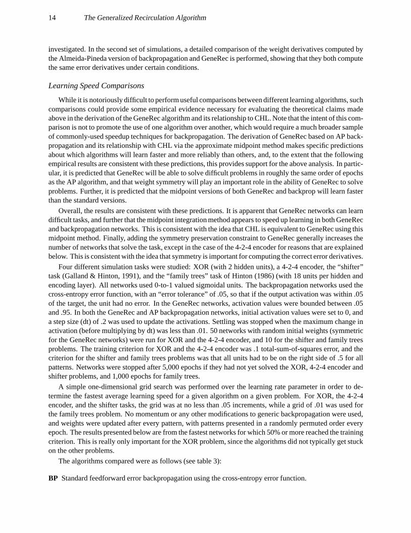
The algorithms compared were as follows (see table 3):

BP Standard feedforward error backpropagation using the cross-entropy error function.

O’Reilly 15

Euler MidpointErr Method FF vs. Rec NonSym Sym NonSym Sym

BP FF BP — BP Mid —Rec AP — — —

Act Diff FF — — — —Rec GR GR Sym GR Mid CHL

Table 3: Relationship of the algorithms tested with respect to the use of local activations vs. explicit backpropagation(BP, Act Diff) to compute error derivatives, feedforward vs. recurrent (FF, Rec), forward Euler vs. the midpoint method(Euler, Midpoint), and weight symmetrization (NonSym, Sym). GR is GeneRec.

AP Almeida-Pineda backpropagation in a recurrent network using the cross-entropy error function.

BP Mid Wt Feedforward error backpropagation with the weight-based version of the approximate midpoint(27). Several different values of the trial step size parameter

^ �� were used in order to determine theeffects of overestimating the trial step as is the case with GeneRec. The values were: 1, 5, 10, and 25for XOR and the 4-2-4 encoder, .5, 1, and 2 for the shifter problem, and .05, .1, .2, and .5 for the familytrees problem. The large trial step sizes resulted in faster learning in small networks, but progressivelysmaller step sizes were necessary for the larger problems.

BP Mid Un Feedforward error backpropagation with the unit-error based version of the midpoint integra-tion method (28). The same trial step size parameters as in BP Mid Wt were used.

GR The basic GeneRec algorithm (17).

GR Sym GeneRec with the symmetry preservation constraint (20).

GR Mid GeneRec with the approximate midpoint method (18).

CHL GeneRec with both symmetry and approximate midpoint method, which is equivalent to CHL (7).

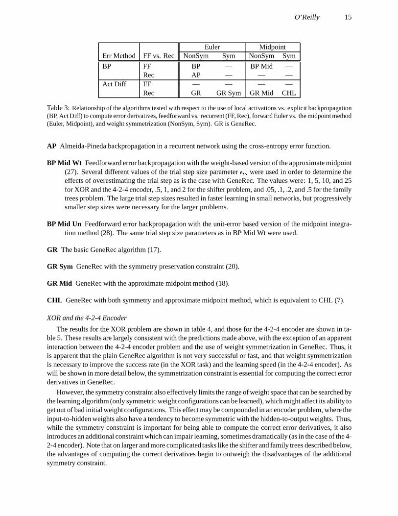
XOR and the 4-2-4 Encoder

The results for the XOR problem are shown in table 4, and those for the 4-2-4 encoder are shown in ta-ble 5. These results are largely consistent with the predictions made above, with the exception of an apparentinteraction between the 4-2-4 encoder problem and the use of weight symmetrization in GeneRec. Thus, itis apparent that the plain GeneRec algorithm is not very successful or fast, and that weight symmetrizationis necessary to improve the success rate (in the XOR task) and the learning speed (in the 4-2-4 encoder). Aswill be shown in more detail below, the symmetrization constraint is essential for computing the correct errorderivatives in GeneRec.

However, the symmetry constraint also effectively limits the range of weight space that can be searched bythe learning algorithm (only symmetric weight configurations can be learned), which might affect its ability toget out of bad initial weight configurations. This effect may be compounded in an encoder problem, where theinput-to-hidden weights also have a tendency to become symmetric with the hidden-to-output weights. Thus,while the symmetry constraint is important for being able to compute the correct error derivatives, it alsointroduces an additional constraint which can impair learning, sometimes dramatically (as in the case of the 4-2-4 encoder). Note that on larger and more complicated tasks like the shifter and family trees described below,the advantages of computing the correct derivatives begin to outweigh the disadvantages of the additionalsymmetry constraint.


Algorithm^

N Epcs SEM

BP 1.95 37 305 58AP 1.40 35 164 23BP Mid Wt 1 1.85 39 268 59BP Mid Wt 5 0.25 25 326 79BP Mid Wt 10 0.25 34 218 25BP Mid Wt 25 0.35 27 215 40BP Mid Un 1 1.40 40 222 28BP Mid Un 5 1.05 34 138 38BP Mid Un 10 0.40 26 222 10BP Mid Un 25 0.30 31 178 37GR 0.20 ¡8¢ 3795 267GR Sym 0.60 31 334 7.1GR Mid 1.75 33 97 4.6CHL 1.80 28 59 1.8

Table 4: Results for the XOR problem. £ is the optimal learning rate, N is the number of networks that successfullysolved the problem (out of 50, minimum of 25), Epcs is the mean number of epochs required to reach criterion, and SEMis the standard error of this mean. Algorithms are as described in the text. ¤ Note that this was the best performancefor the GR networks.

Algorithm^

N Epcs SEM

BP 2.40 50 60 5.1AP 2.80 50 54 3.6BP Mid Wt 1 1.70 50 60 4.3BP Mid Wt 5 1.65 50 48 2.8BP Mid Wt 10 2.35 50 45 3.6BP Mid Wt 25 2.25 50 37 3.0BP Mid Un 1 2.20 50 54 4.2BP Mid Un 5 2.10 50 42 2.5BP Mid Un 10 2.10 50 40 2.9BP Mid Un 25 1.95 50 34 1.8GR 0.60 45 418 28GR Sym 1.40 28 88 2.9GR Mid 2.40 46 60 3.4CHL 1.20 28 77 1.8

Table 5: Results for the 4-2-4 encoder problem. £ is the optimal learning rate, N is the number of networks that suc-cessfully solved the problem (out of 50), minimum of 25, Epcs is the mean number of epochs required to reach criterion,and SEM is the standard error of this mean. Algorithms are as described in the text.

O’Reilly 17

The other main prediction from the analysis is that the approximate midpoint method will result in fasterlearning, both in BP and GeneRec. This appears to be the case, where the speedup relative to regular back-prop was nearly two-fold for the unit-error based version with a trial step size of 25. The general advantageof the unit-error over the weight based midpoint method in BP is interesting considering that this correspondsto the GeneRec version of the midpoint method. The speedup in GeneRec for both the CHL vs GR Sym andGR Mid vs GR comparisons was substantial in general. Further, it is interesting that the approximate mid-point method alone (without the symmetrization constraint) can enable the GeneRec algorithm to success-fully solve problems. Indeed, on both of these tasks, GR Mid performed better than GR Sym. This might beattributable to the ability of the midpoint method to compute better weight derivatives which are less affectedby the inaccuracies introduced by the lack of weight symmetry. However, note that while this seems to holdfor all of the three-layer networks studied, it breaks down in the family trees task which requires error deriva-tives to be passed back through multiple hidden layers. Also, only on the 4-2-4 encoder did GR Mid performbetter than CHL, indicating that there is generally an advantage to having the correct error derivatives viaweight symmetrization in addition to using the midpoint method.

An additional finding is that there appears to be an advantage for the use of a recurrent network over a feed-forward one, based on a comparison of AP vs BP results. This can be explained by the fact that small weightchanges in a recurrent network can lead to more dramatic activation state differences than in a feedforwardnetwork. In effect, the recurrent network has to do less work to achieve a given set of activation states thandoes a feedforward network. This advantage for recurrency, which should be present in GeneRec, is prob-ably partially offset by the additional weight symmetry constraint. Further, recurrency appears to become aliability in networks with multiple hidden layers, based on the family trees results presented below.

The Shifter Task

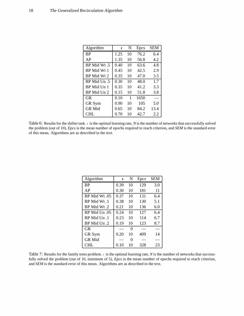
The shifter problem is a larger task than XOR and the 4-2-4 encoder, and thus might provide a morerealistic barometer of performance on typical tasks. ¥ The version of the shifter problem used here had two4 bit input patterns, one of which was a shifted version of the other. There were three values of shift, -1, 0,and 1, corresponding to one bit to the left, the same, and one bit to the right (with wrap-around). Of the 16possible binary patterns on 4 bits, 4 were unsuitable because they result in the same pattern when shifted rightor left (1111, 1010, 0101, and 0000). Thus, there were 36 training patterns (the 12 bit patterns shifted in eachof 3 directions). The task was to classify the shift direction by activating one of 3 output units. While largerversions of this task (more levels of shift, more bits in the input) were explored, this configuration provedthe most difficult (in terms of epochs) for a standard BP network to solve.

The results, shown in table 6, provide clearer support for the predicted relationships than the two previ-ous tasks. In particular, the midpoint-based speedup is comparable between the BP and GeneRec cases, andthe role of symmetry in GeneRec is unambiguously important for solving the task, as is evident from the al-most complete failure of the non-symmetric version to learn the problem. However, it is interesting that evenin this more complicated problem the use of the approximate midpoint method without the additional sym-metrizing constraint enables the GeneRec networks to learn the problem. Nevertheless, the combination ofthe approximate midpoint method and the symmetrizing constraint (i.e., the CHL algorithm) performs betterthan either alone.

As in the previous tasks, there appears to be an advantage for the use of a recurrent network over a non-recurrent one, as evidenced by the faster learning of AP compared to BP.

The Family Trees Task

As was mentioned in the introduction, the family trees task of Hinton (1986) is of particular interest be-cause Galland (1993) reported that he was unable to train CHL to solve this problem. While I was unable to¦

Note that other common tasks like digit recognition or other classification tasks were found to be so easily solved by a standardBP network (under 10 epochs), that they did not provide a useful dynamic range to make the desired comparisons.


Algorithm^

N Epcs SEM

BP 1.25 10 76.2 6.4AP 1.35 10 56.8 4.2BP Mid Wt .5 0.40 10 63.6 4.8BP Mid Wt 1 0.45 10 42.5 2.9BP Mid Wt 2 0.35 10 47.0 3.5BP Mid Un .5 0.30 10 48.0 1.7BP Mid Un 1 0.35 10 41.2 3.3BP Mid Un 2 0.15 10 51.8 3.8GR 0.10 1 1650 —GR Sym 0.90 10 105 5.0GR Mid 0.65 10 84.2 13.4CHL 0.70 10 42.7 2.2

Table 6: Results for the shifter task. £ is the optimal learning rate, N is the number of networks that successfully solvedthe problem (out of 10), Epcs is the mean number of epochs required to reach criterion, and SEM is the standard errorof this mean. Algorithms are as described in the text.

Algorithm^

N Epcs SEM

BP 0.39 10 129 3.0AP 0.30 10 181 11BP Mid Wt .05 0.37 10 131 6.4BP Mid Wt .1 0.38 10 130 5.1BP Mid Wt .2 0.21 10 136 6.0BP Mid Un .05 0.24 10 127 6.4BP Mid Un .1 0.23 10 114 6.7BP Mid Un .2 0.19 10 123 8.7GR — 0 — —GR Sym 0.20 10 409 14GR Mid — 0 — —CHL 0.10 10 328 23

Table 7: Results for the family trees problem. £ is the optimal learning rate, N is the number of networks that success-fully solved the problem (out of 10, minimum of 5), Epcs is the mean number of epochs required to reach criterion,and SEM is the standard error of this mean. Algorithms are as described in the text.

O’Reilly 19

get§ a CHL network to learn the problem with the same number of hidden units as was used in the originalbackprop version of this task (6 “encoding” units per input/output layer, and 12 central hidden units), simplyincreasing the number of encoding units to 12 was enough to allow CHL to learn the task, although not with100% reliability. Thus, the learning rate search was performed on networks with 18 encoding and 18 hiddenunits to ensure that networks were capable of learning.

As can be seen from the results shown in table 7, the CHL networks were able to reliably solve thistask within a roughly comparable number of epochs as the AP networks. Note that the recurrent networks(GeneRec and AP) appear to be at a disadvantage relative to feedforward BP ¨ on this task, probably due tothe difficulty of shaping the appropriate attractors over multiple hidden layers. Also, symmetry preservationappears to be critical for GeneRec learning in deep networks, since GeneRec networks without this wereunable to solve this task (even with the midpoint method).

The comparable performance of AP and CHL supports the derivation of CHL via the GeneRec algorithmas essentially a form of backpropagation, and calls into question the analyses of Galland (1993) regardingthe limitations of CHL as a deterministic approximation to a Boltzmann machine. It is difficult to determinewhat is responsible for the failure to learn the family trees problem reported in Galland (1993), since there areseveral differences in the way those networks were run compared to the ones described above, including theuse of an annealing schedule, not using the .05, .95 activation cutoff, using activations with -1 to +1 range,using batch mode instead of on-line weight updating, and using activation-based as opposed to net-input-based settling.

Finally, only the unit-error based midpoint method in backpropagation showed a learning speed advantagein this task. This is consistent with the trend of the previous results. The advantage of the unit-error basedmidpoint method might be due to the reliance on the derivative of the error with respect to the hidden unititself, which could be a more reliable indication of the curvature of the derivative than the weight derivativesused in the other method.

The GeneRec Approximation to AP BP

The analysis presented earlier in the paper shows that GeneRec should compute the same error derivativesas the Almeida-Pineda version of error backpropagation in a recurrent network if the following conditionshold:� The difference of the plus and minus phase activation terms in GeneRec, which are updated in separate

iterative activation settling phases, can be used to compute a unit’s error term instead of the iterativeupdate of the difference itself, which is what Almeida-Pineda uses.� The reciprocal weights are symmetric. This enables the activation signals from the output to the hiddenunits (via the recurrent weights) to reflect the contribution that the hidden units made to the output error(via the forward-going weights).� The difference of activations in the plus and minus phases is a reasonable approximation to the differ-ence of net inputs times the derivative of the sigmoidal activation function. Note that this only affectsthe overall magnitude of the weight derivatives, not their direction.

In order to evaluate the extent to which these conditions are violated and the effect that this has on learningin GeneRec, two identical networks were run side-by-side on the same sequence of training patterns, with one©

It should be noted that the performance of feedforward BP on this task is much faster than previously reported results. This ismost likely due to the use of on-line learning and not using momentum, which enables the network to take advantage of the noisedue to the random order of the training patterns to break the symmetry of the error signals generated in the problem and distinguishamongst the different training patterns.


0ª

100ª

200ª

300ª

400ª

500ª

600ª

700ª

800ª

900ª

1000ª

Epochs of Training«0.0

0.1

0.2

0.3

0.4

0.5

0.6

0.7

0.8

0.9

1.0

Dot

Pro

du

ct o

r N

orm

SS

E

¬

GeneRec vs. Almeida-PinedaStuck Net, Yoked to GeneRec, Brute-force Symmetrization6®

I->H dWt Dot Product ¯SSE (Normalized)°

0±

20±

40±

60±

80±

100±

120² 140³ 160´Epochs of Trainingµ0.0

0.1

0.2

0.3

0.4

0.5

0.6

0.7

0.8

0.9

1.0

Dot

Pro

du

ct o

r N

orm

SS

E

¶

GeneRec vs. Almeida-PinedaFast Net, Yoked to GeneRec, Brute-force Symmetrization

I->H dWt Dot Product ·SSE (Normalized)¸

b)a)

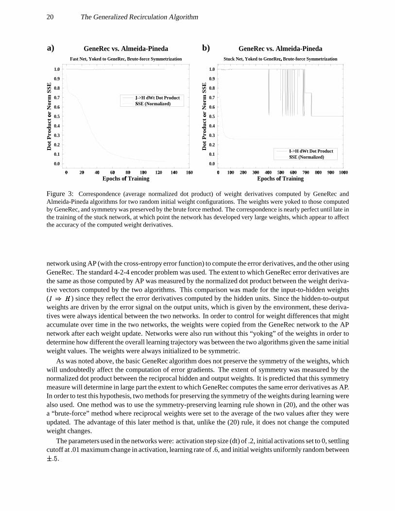
Figure 3: Correspondence (average normalized dot product) of weight derivatives computed by GeneRec andAlmeida-Pineda algorithms for two random initial weight configurations. The weights were yoked to those computedby GeneRec, and symmetry was preserved by the brute force method. The correspondence is nearly perfect until late inthe training of the stuck network, at which point the network has developed very large weights, which appear to affectthe accuracy of the computed weight derivatives.

network using AP (with the cross-entropy error function) to compute the error derivatives, and the other usingGeneRec. The standard 4-2-4 encoder problem was used. The extent to which GeneRec error derivatives arethe same as those computed by AP was measured by the normalized dot product between the weight deriva-tive vectors computed by the two algorithms. This comparison was made for the input-to-hidden weights( ¹kº¼» ) since they reflect the error derivatives computed by the hidden units. Since the hidden-to-outputweights are driven by the error signal on the output units, which is given by the environment, these deriva-tives were always identical between the two networks. In order to control for weight differences that mightaccumulate over time in the two networks, the weights were copied from the GeneRec network to the APnetwork after each weight update. Networks were also run without this “yoking” of the weights in order todetermine how different the overall learning trajectory was between the two algorithms given the same initialweight values. The weights were always initialized to be symmetric.

As was noted above, the basic GeneRec algorithm does not preserve the symmetry of the weights, whichwill undoubtedly affect the computation of error gradients. The extent of symmetry was measured by thenormalized dot product between the reciprocal hidden and output weights. It is predicted that this symmetrymeasure will determine in large part the extent to which GeneRec computes the same error derivatives as AP.In order to test this hypothesis, two methods for preserving the symmetry of the weights during learning werealso used. One method was to use the symmetry-preserving learning rule shown in (20), and the other wasa “brute-force” method where reciprocal weights were set to the average of the two values after they wereupdated. The advantage of this later method is that, unlike the (20) rule, it does not change the computedweight changes.

The parameters used in the networks were: activation step size (dt) of .2, initial activations set to 0, settlingcutoff at .01 maximum change in activation, learning rate of .6, and initial weights uniformly random between½¿¾ÁÀ

.

O’Reilly 21

0Â

50Â

100Â

150Ã 200Â

250ÃEpochs of TrainingÄ0.0

0.1

0.2

0.3

0.4

0.5

0.6

0.7

0.8

0.9

1.0

Dot

Pro

du

ct o

r N

orm

SS

E

Å

GeneRec vs. Almeida-PinedaMedium Net, Yoked to GeneRec, No Symmetrization

I->H dWt Dot Product ÆRecip Wts Dot ProductÇSSE (Normalized)

0±

20±

40±

60±

80±

100±

120²Epochs of Trainingµ0.0

0.1

0.2

0.3

0.4

0.5

0.6

0.7

0.8

0.9

1.0

Dot

Pro

du

ct o

r N

orm

SS

E

¶

GeneRec vs. Almeida-PinedaFast Net, Yoked to GeneRec, No Symmetrization

I->H dWt Dot Product ·Recip Wts Dot ProductÈSSE (Normalized)¸

b)a)

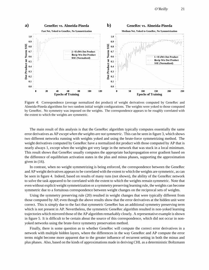
Figure 4: Correspondence (average normalized dot product) of weight derivatives computed by GeneRec andAlmeida-Pineda algorithms for two random initial weight configurations. The weights were yoked to those computedby GeneRec. No symmetry was imposed on the weights. The correspondence appears to be roughly correlated withthe extent to which the weights are symmetric.

The main result of this analysis is that the GeneRec algorithm typically computes essentially the sameerror derivatives as AP except when the weights are not symmetric. This can be seen in figure 3, which showstwo different networks running with weights yoked and using the brute-force symmetrizing method. Theweight derivatives computed by GeneRec have a normalized dot product with those computed by AP that isnearly always 1, except when the weights got very large in the network that was stuck in a local minimum.This result shows that GeneRec usually computes the appropriate backpropagation error gradient based onthe difference of equilibrium activation states in the plus and minus phases, supporting the approximationgiven in (16).

In contrast, when no weight symmetrizing is being enforced, the correspondence between the GeneRecand AP weight derivatives appears to be correlated with the extent to which the weights are symmetric, as canbe seen in figure 4. Indeed, based on results of many runs (not shown), the ability of the GeneRec networkto solve the task appeared to be correlated with the extent to which the weights remain symmetric. Note thateven without explicit weight symmetrization or a symmetry preserving learning rule, the weights can becomesymmetric due to a fortuitous correspondence between weight changes on the reciprocal sets of weights.

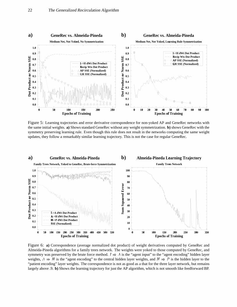
Using the symmetry preserving rule (20) resulted in weight changes that were typically different fromthose computed by AP, even though the above results show that the error derivatives at the hidden unit werecorrect. This is simply due to the fact that symmetric GeneRec has an additional symmetry preserving termwhich is not present in AP. Nevertheless, the symmetric GeneRec algorithm resulted in non-yoked learningtrajectories which mirrored those of the AP algorithm remarkably closely. A representative example is shownin figure 5. It is difficult to be certain about the source of this correspondence, which did not occur in non-yoked networks using the brute-force symmetry preservation method.

Finally, there is some question as to whether GeneRec will compute the correct error derivatives in anetwork with multiple hidden layers, where the differences in the way GeneRec and AP compute the errorterms might become more apparent due to the greater influence of recurrent setting in both the minus andplus phases. Also, based on the kinds of approximations made in deriving CHL as a deterministic Boltzmann


0±

10±

20±

30±

40±

50±

60±

70±

80±

90±

100±

Epochs of Trainingµ0.0

0.1

0.2

0.3

0.4

0.5

0.6

0.7

0.8

0.9

1.0

Dot

Pro

du

ct o

r N

orm

SS

E

¶

GeneRec vs. Almeida-PinedaMedium Net, Not Yoked, Learning Rule SymmetrizationÉ

I->H dWt Dot Product ·Recip Wts Dot ProductÈAP SSE (Normalized)ÊGR SSE (Normalized)Ë

0Ì

50Ì

100Ì

150Í 200Ì

250ÍEpochs of TrainingÎ0.0

0.1

0.2

0.3

0.4

0.5

0.6

0.7

0.8

0.9

1.0

Dot

Pro

du

ct o

r N

orm

SS

E

Ï

GeneRec vs. Almeida-PinedaMedium Net, Not Yoked, No SymmetrizationÐ

I->H dWt Dot Product ÑRecip Wts Dot ProductÒAP SSE (Normalized)ÓGR SSE (Normalized)

b)a)

Figure 5: Learning trajectories and error derivative correspondence for non-yoked AP and GeneRec networks withthe same initial weights. a) Shows standard GeneRec without any weight symmetrization. b) shows GeneRec with thesymmetry preserving learning rule. Even though this rule does not result in the networks computing the same weightupdates, they follow a remarkably similar learning trajectory. This is not the case for regular GeneRec.

0Ô

50Ô

100Ô

150Õ 200Ô

250Õ 300Ô

350ÕEpochs of Training

0

10

20

30

40

50

60

70

80

90

100

Su

m S

qu

ared

Err

or

Ö

Almeida-Pineda Learning Trajectory×Family Trees NetworkØ

0Ù

50Ù

100Ù

150Ú 200Ù

250Ú 300Ù

350Ú 400Ù

450Ú 500Ù

550ÚEpochs of Training

0.0

0.1

0.2

0.3

0.4

0.5

0.6

0.7

0.8

0.9

1.0

Dot

Pro

du

ct o

r N

orm

SS

E

Û

GeneRec vs. Almeida-PinedaÜFamily Trees Network, Yoked to GeneRec, Brute-force SymmetrizationÝ

I->A dWt Dot Product ÞA->H dWt Dot ProductßH->P dWt Dot ProductàSSE (Normalized)á

b)a)

Figure 6: a) Correspondence (average normalized dot product) of weight derivatives computed by GeneRec andAlmeida-Pineda algorithms for a family trees network. The weights were yoked to those computed by GeneRec, andsymmetry was preserved by the brute force method. âDãåä is the “agent input” to the “agent encoding” hidden layerweights, äbãçæ is the “agent encoding” to the central hidden layer weights, and æåãéè is the hidden layer to the“patient encoding” layer weights. The correspondence is not as good as a that for the three layer network, but remainslargely above .9. b) Shows the learning trajectory for just the AP algorithm, which is not smooth like feedforward BP.

O’Reilly 23

machine,ê and the results of simulations, Galland (1993) concluded that the limitations of CHL become moreapparent as the number of hidden layers are increased (i.e., in “deep” networks).

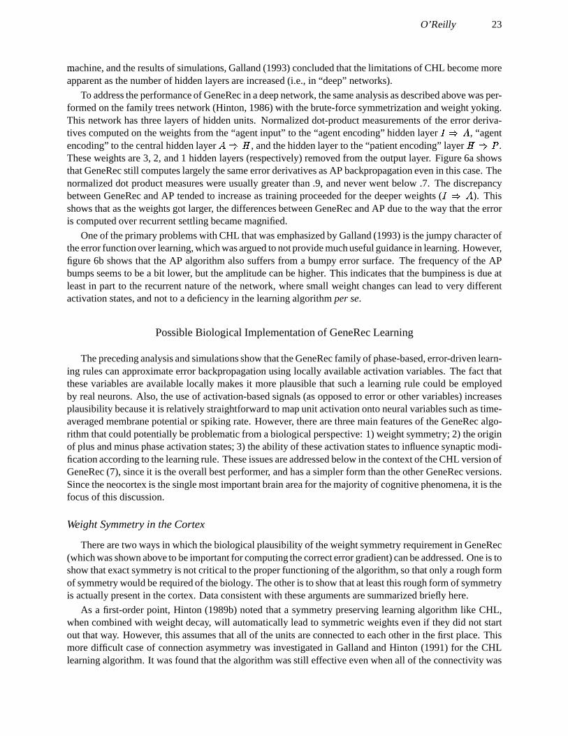
To address the performance of GeneRec in a deep network, the same analysis as described above was per-formed on the family trees network (Hinton, 1986) with the brute-force symmetrization and weight yoking.This network has three layers of hidden units. Normalized dot-product measurements of the error deriva-tives computed on the weights from the “agent input” to the “agent encoding” hidden layer ëíìïî , “agentencoding” to the central hidden layer îbìçð , and the hidden layer to the “patient encoding” layer ðñìéò .These weights are 3, 2, and 1 hidden layers (respectively) removed from the output layer. Figure 6a showsthat GeneRec still computes largely the same error derivatives as AP backpropagation even in this case. Thenormalized dot product measures were usually greater than .9, and never went below .7. The discrepancybetween GeneRec and AP tended to increase as training proceeded for the deeper weights ( ësìóî ). Thisshows that as the weights got larger, the differences between GeneRec and AP due to the way that the erroris computed over recurrent settling became magnified.

One of the primary problems with CHL that was emphasized by Galland (1993) is the jumpy character ofthe error function over learning, which was argued to not provide much useful guidance in learning. However,figure 6b shows that the AP algorithm also suffers from a bumpy error surface. The frequency of the APbumps seems to be a bit lower, but the amplitude can be higher. This indicates that the bumpiness is due atleast in part to the recurrent nature of the network, where small weight changes can lead to very differentactivation states, and not to a deficiency in the learning algorithm per se.

Possible Biological Implementation of GeneRec Learning

The preceding analysis and simulations show that the GeneRec family of phase-based, error-driven learn-ing rules can approximate error backpropagation using locally available activation variables. The fact thatthese variables are available locally makes it more plausible that such a learning rule could be employedby real neurons. Also, the use of activation-based signals (as opposed to error or other variables) increasesplausibility because it is relatively straightforward to map unit activation onto neural variables such as time-averaged membrane potential or spiking rate. However, there are three main features of the GeneRec algo-rithm that could potentially be problematic from a biological perspective: 1) weight symmetry; 2) the originof plus and minus phase activation states; 3) the ability of these activation states to influence synaptic modi-fication according to the learning rule. These issues are addressed below in the context of the CHL version ofGeneRec (7), since it is the overall best performer, and has a simpler form than the other GeneRec versions.Since the neocortex is the single most important brain area for the majority of cognitive phenomena, it is thefocus of this discussion.

Weight Symmetry in the Cortex

There are two ways in which the biological plausibility of the weight symmetry requirement in GeneRec(which was shown above to be important for computing the correct error gradient) can be addressed. One is toshow that exact symmetry is not critical to the proper functioning of the algorithm, so that only a rough formof symmetry would be required of the biology. The other is to show that at least this rough form of symmetryis actually present in the cortex. Data consistent with these arguments are summarized briefly here.

As a first-order point, Hinton (1989b) noted that a symmetry preserving learning algorithm like CHL,when combined with weight decay, will automatically lead to symmetric weights even if they did not startout that way. However, this assumes that all of the units are connected to each other in the first place. Thismore difficult case of connection asymmetry was investigated in Galland and Hinton (1991) for the CHLlearning algorithm. It was found that the algorithm was still effective even when all of the connectivity was


asymmetricô (i.e., for each pair of non-input units, only one of the two possible connections between themexisted). This robustness can be attributed to a redundancy in the ways in which the error signal informationcan be obtained (i.e., a given hidden unit could obtain the error signal directly from the output units, or indi-rectly through connections to other hidden units). Also, note that the absence of any connection at all is verydifferent from the presence of connection with a non-symmetric weight value, which is the form of asym-metry that was found to be problematic in the above analysis. In the former case, only a subset of the errorgradient information is available, while the latter case can result in specifically wrong gradient informationdue to the influence of the non-symmetric weight. Due to the automatic symmetrization property of CHL,the latter case is unlikely to be a problem.

In terms of biological evidence for symmetric connectivity, there is some indication that the cortex is atleast roughly symmetrically connected. At the level of identifiable anatomical subregions of cortex, the vastmajority of areas (at least within the visual cortex) are symmetrically connected to each other. That is, if areaA projects to area B, area A also receives a projection from area B (Felleman & Van Essen, 1991). At thelevel of cortical columns or “stripes” within the prefrontal cortex of the monkey, Levitt, Lewis, Yoshioka,and Lund (1993) showed that connectivity was symmetric between interconnected stripes. Thus, if a neuronreceived projections from neurons in a given stripe, it also projected to neurons in that stripe. The moredetailed level of individual neuron symmetric connectivity is difficult to assess empirically, but there is atleast no evidence that it does not exist. Further, given that there is evidence for at least rough symmetry,detailed symmetry may not be critical since, as demonstrated by Galland and Hinton (1991), CHL can useasymmetrical connectivity as long as there is some way of obtaining reciprocal information through a subsetof symmetric connections or indirectly via other neurons in the same area.

Phase-Based Activations in the Cortex

The origin of the phase-based activations that are central to the GeneRec algorithm touches at the heart ofperhaps the most controversial aspect of error-driven learning in the cortex: “where does the teaching signalcome from?” In GeneRec, the teaching signal is just the plus-phase activation state. Thus, unlike standardbackpropagation, GeneRec suggests that the teaching signal is just another state of “experience” in the net-work. One can interpret this state as that of experiencing the actual outcome of some previous conditions.Thus, the minus phase can be thought of as the expectation of the outcome given these conditions. For ex-ample, after hearing the first three words of a sentence, an expectation will develop of which word is likely tocome next. The state of the neurons upon generating this expectation is the minus phase. The experience ofhearing or reading the actual word that comes next establishes a subsequent locomotive õ state of activation,which serves as the plus phase. This idea that the brain is constantly generating expectations about subse-quent events, and that the discrepancies between these expectations and subsequent outcomes can be usedfor error-driven learning, has been suggested by McClelland (1994) as a psychological interpretation of thebackpropagation learning procedure. It is particularly attractive for the GeneRec version of backpropaga-tion, which uses only activation states, because it requires no additional mechanisms for providing specificteaching signals other than the effects of experience on neural activation states in a manner that is widelybelieved to be taking place in the cortex anyway.

Further, there is evidence from ERP recordings of electrical activity over the scalp during behavioral tasksthat cortical activation states reflect expectations and are sensitive to differential outcomes. For example, thewidely-studied P300 wave, which is a positive-going wave that occurs around 300 msec after stimulus onset,is considered to measure a violation of subjective expectancy which is determined by preceding experienceover both the short and long term (Hillyard & Picton, 1987). In more formal terms, Sutton, Braren, Zubin, andJohn (1965) showed that the P300 amplitude is determined by the amount of prior uncertainty that is resolvedö

This is just to demonstrate that such expectations are being generated and it is salient when they are violated.

O’Reilly 25

Minus Phase VariablesPlus Phase Variables ÷`øù ÷úøû�ü�ý ( þÁÿ ÷ �� ù near 0) ÷úøù ÷`øû[ü�� ( þÁÿ ÷ �� ù elevated)÷ �ù ÷ �û ü�ý �� ù û� ý �� ùÁû� �� (LTD)÷ �ù ÷ �û[ü�� ù û� �� (LTP) �� ù û� ý��

Table 8: Directions of weight change according to the CHL rule for four qualitative conditions, consisting of the com-binations of two qualitative levels of minus and plus phase activation coproduct values. The minus phase activation co-product is thought to correspond to ��! . Increases in synaptic efficacy correspond to long-term potentiation (LTP)and decreases are long-term depression (LTD). " This cell is not consistent with the biological mechanism because both��#�! and synaptic activity lead to LTP, not the absence of LTP. See text for a discussion of this point.

by the processing of a given event. Thus, the nature of the P300 is consistent with the idea that it representsa plus phase wave of activation following in a relatively short time-frame the development of minus phaseexpectations. While the specific properties of the P300 itself might be due to specialized neural mechanismsfor monitoring discrepancies between expectations and outcomes, its presence suggests the possibility thatneurons in the mammalian neocortex experience two states of activation in relatively rapid succession, onecorresponding to expectation and the other corresponding to outcome.

Finally, note that for most of the GeneRec variants, it seems that the neuron needs to have both the plusand minus phase activation signals in reasonably close temporal proximity in order to adjust its synapsesbased on both values. This is consistent with the relatively rapid expectation-outcome interpretation givenabove. However, CHL is a special case, since it is simply the difference between the coproduct of same-phase activations, which could potentially be computed by performing simple Hebbian associative learningfor the plus phase at any point, and at any other point, performing anti-Hebbian learning on the minus phaseactivations (Hinton & Sejnowski, 1986). This leaves open the problems of how the brain would know when tochange the sign of the weight change, and how this kind of global switch could be implemented. Also, peopleare capable of learning things relatively quickly (within seconds or at least minutes), so this phase switchingis unlikely to be a function of the difference between REM sleep and waking behavior, as has been suggestedfor phase-based learning algorithms (Hinton & Sejnowski, 1986; Linsker, 1992; Crick & Mitchison, 1983).While it might be possible to come up with answers to these problems, a temporally local mechanism likethat suggested above seems more plausible.

Synaptic Modification Mechanisms

Having suggested that the minus and plus phase activations follow each other in rapid succession, it re-mains to be shown how these two activation states could influence synaptic modification in a manner largelyconsistent with the CHL version of GeneRec (7). It turns out that the biological mechanism proposed belowaccounts for only three out of four different qualitative ranges of the sign of the weight change required byCHL (see table 8). Specifically, the proposed mechanism predicts weight increase to occur when both thepre and postsynaptic neurons are active in both the plus and minus phases, whereas CHL predicts that theweight change in this condition should be zero. Thus, the proposed mechanism corresponds to a combina-tion of CHL and a Hebbian-style learning rule, the computational implications of which are the subject ofO’Reilly (1996), which shows that the combination of error-driven and associative learning can be generallybeneficial for solving many different kinds of tasks.

To briefly summarize the findings of O’Reilly (1996), the Hebbian component can be thought of as impos-ing additional constraints on learning much in the way that weight decay is used in conjunction with standarderror backpropagation. However, the constraints imposed by Hebbian learning are actually capable of pro-ducing useful representations on their own (unlike weight decay, which would simply reduce all weights tozero if left to its own devices). Thus, the combination of CHL and Hebbian learning results in networks that,


unlike$ those with weight decay, learn faster (especially in deep networks like the family trees task), and gen-eralize better (due to the effects of the additional constraints) than plain CHL networks. However, for thepurposes of the present paper, the crucial aspect of the following mechanism is that it provides the error cor-rection term, which occurs when the synaptic coproduct ÷ ù ÷ û was larger in the minus phase than in the plusphase. This is the defining aspect of the error-driven learning performed by CHL, since the other qualitativeranges of the CHL learning rule are similar to standard Hebbian learning, as is evident from table 8.

For GeneRec-style learning to occur at a cellular and synaptic level, the neuron needs to be able to retainsome trace of the minus phase activation state through the time when the neuron experiences its plus phaseactivation state. Reasoning from the ERP data described above, this time period might be around 300 mil-liseconds or so. A likely candidate for the minus phase trace is intracellular ÿ ÷ �� ( þÁÿ¿÷ �� ù ), which entersthe postsynaptic area via NMDA channels if both pre and postsynaptic neurons are active. To implement aGeneRec-style learning rule, this minus phase þÁÿ¿÷ �� ù trace needs to interact with the subsequent plus phaseactivity to determine if the synapse is potentiated (LTP) or depressed (LTD). In what follows, the term synap-tic activity will be used to denote the activation coproduct term ÷ ù ÷ û , which is effectively what determinesthe amount of þÁÿ¿÷ ��%� ù that enters through the NMDA channel (Collingridge & Bliss, 1987).

There are two basic categories of mechanism which can provide the crucial error-correcting modulationof the sign of synaptic modification required by CHL. One such mechanism involves an interaction betweenmembrane potential or synaptic activity and þ ÿ¿÷ �� ù , while another depends only on the level of þÁÿ¿÷ �� ù .Further, there are many ways in which these signals and their timing can affect various second-messengersystems in the cell to provide the necessary modulation. In favor of something like the first mechanism, thereis evidence that the mere presence of postsynaptic þÁÿ¿÷ �� ù is insufficient to cause LTP (Kullmann, Perkel,Manabe, & Nicoll, 1992; Bashir, Bortolotto, & Davies, 1993), but it is unclear exactly what additional factoris necessary (Bear & Malenka, 1994). One hypothesis is that LTP depends on the activation of metabotropicglutamate receptors, which are activated by presynaptic activity and can trigger various mechanisms in thepostsynaptic synaptic compartment (Bashir et al., 1993). On the other hand, a proposed mechanism that de-pends only on the level of postsynaptic þÁÿ¿÷ �� ù (Lisman, 1989), has received some recent empirical support(reviewed in Lisman, 1994; Bear & Malenka, 1994). This proposal stipulates that increased but moderateconcentrations of postsynaptic þÁÿ ÷ �� ù lead to LTD, while higher concentrations lead to LTP. Artola andSinger (1993) argue that this mechanism is consistent with the ABS learning rule (Hancock, Smith, & Phillips,1991; Artola, Brocher, & Singer, 1990; Bienenstock, Cooper, & Munro, 1982), which stipulates that thereare two thresholds for synaptic modification, & � and & ø . A level of þÁÿ ÷ �� ù which is higher than the highthreshold & � leads to LTP, while a level which is lower than this high threshold but above the lower & øthreshold leads to LTD.

Either of the above mechanisms would be capable of producing the pattern of synaptic modification shownin table 8 in the context of a proposed mechanism defined by the following properties:

1. Some minimal level of þÁÿ ÷ �� ù is necessary for any form of synaptic modification (LTP or LTD).

2. þÁÿ¿÷ �� ù changes relatively slowly, and persists for at least 300+ milliseconds. This allows þÁÿ ÷ �� ù torepresent prior minus phase activity, even if the synapse is not subsequently active in the plus phase.

3. Synaptic modification occurs based on the postsynaptic state after plus phase activity. This can happenlocally if synaptic modification occurs after around 300+ milliseconds since the entry of ÿ ÷ �� into thepostsynaptic area (and the plus phase activity states last for at least this long). Alternatively, there couldbe a relatively global signal corresponding to the plus phase that triggers synaptic modification (e.g., asprovided by dopaminergic or cholinergic modulation triggered by systems sensitive to the experienceof outcomes following expectations).

4. If þÁÿ¿÷ �� ù was present initially (in the minus phase) due to synaptic activity, but then the synaptic

O’Reilly 27

activity diminished or ceased (in the plus phase), LTD should occur. This would be expected from themechanisms described above, either because of an explicit interaction between synaptic activity at thetime of modification in the plus phase and the trace of þÁÿ¿÷ �� ù from the minus phase, or because theminus phase þÁÿ¿÷ �� ù will have decayed into the LTD range by the time modification occurs in the plusphase.

5. If synaptic activity is taking place in the plus phase state, sufficient þ ÿ¿÷ �� ù is present and LTP occurs.Note that this means that any time the plus-phase activation coproduct ( ÷ �ù ÷ �û ) is reasonably large,regardless of whether there was any prior minus phase activity, the weights will be increased. Thisleads to a combined CHL and Hebbian learning rule as discussed above.

There is direct evidence in support of several aspects of the proposed mechanism, some of which wasdiscussed above, and indirect evidence in support of most of the remainder. Since the empirical literature onLTP and LTD is vast, only a brief summary will be given here (see Artola & Singer, 1993; Bear & Malenka,1994; Linden, 1994; Malenka & Nicoll, 1993, for recent reviews). It should be noted that most of thesefindings have been described both in the hippocampus and neocortex, and appear to be quite general (Artola &Singer, 1993; Linden, 1994). Also, note that the NMDA receptor itself is not subject to potentiation, so thatthe current value of the synaptic weight does not have to be included in learning rules, which is in accordancewith GeneRec.

With respect to point 1, the importance of þÁÿ¿÷ �� ù for LTP has been known for a while (e.g., Collingridge &Bliss, 1987), and it is now clear that it is critical for LTD as well (Brocher, Artola, & Singer, 1992; Mulkey &Malenka, 1992; Hirsh & Crepel, 1992). In support of point 2, the time course of þ ÿ¿÷ ��%� ù concentrationhas been measured in several studies (e.g., Jaffe, Johnston, Lasser-Ross, Lisman, Miyakawa, & Ross, 1992;Perkel, Petrozzino, Nicoll, & Connor, 1993), and it appears to be relatively long-lasting (on the order of 1 ormore seconds), though it is not clear that these results reflect what would happen under less invasive condi-tions.

As for point 3, Malenka, Lancaster, and Zucker (1992) found that a significant time period (up to 1-2seconds) of enhanced postsynaptic þ ÿ¿÷ ��%� ù was necessary for LTP induction. Also, typical LTP and LTDinduction regimes involve constant stimulation at a given frequency for time periods longer than a second.However, the precise time course of synaptic potentiation needs to be studied in greater detail to evaluatethis issue fully. With respect to the existence of a global learning signal, the ERP data described earlier andthe role of neuromodulatory systems like dopamine suggest that such monitoring systems might exist in thebrain. For example, Schultz, Apicella, and Ljungberg (1993) describe the important role that dopamine playsin learning and responding to salient environmental stimuli. However, these modulatory effects are probablynot of an all-or-nothing nature, and, given that LTP and LTD can be induced by the direct electrical stimula-tion of individual neurons, it is not likely that learning is completely dependent on a global signal.

To summarize, the proposed synaptic modification mechanism is consistent with several findings, but alsorequires further mechanisms. As such, the proposal outlined above constitutes a set of predictions regardingadditional factors that should determine the sign and magnitude of synaptic modification.

Conclusions

The analysis and simulation results presented in this paper support the idea that the GeneRec family oflearning algorithms are performing variations of error backpropagation in a recurrent network using locallyavailable activation variables. However, there is no single GeneRec algorithm which is exactly equivalent tothe Almeida-Pineda algorithm for backpropagation in recurrent networks since GeneRec requires symmetricweights yet it is not itself symmetry preserving.


The idea that the CHL algorithm is equivalent to a symmetry preserving version of GeneRec using themidpoint integration method is supported by the pattern of learning speed results for the different versionsof GeneRec, and by the learning speed increases obtained when using the approximate midpoint integrationmethod in backpropagation networks. Further, it was shown that CHL (and symmetric GeneRec withoutthe midpoint method) can reliably learn the family trees problem, calling into question the idea that CHL is afundamentally flawed learning algorithm for deterministic networks, as was argued by Galland (1993). Thus,the weight of the evidence suggests that CHL should be viewed as a variation of recurrent backpropagation,not as a poor approximation to the Boltzmann machine learning algorithm.

However, as a consequence of the differences between GeneRec and AP backpropagation (mainly thesymmetry constraint), one can expect GeneRec to have somewhat different characteristics compared to stan-dard backpropagation algorithms, and it may turn out that these differences have implications for psycho-logical or computational models. Thus, the present analysis does not imply that just because there exists abiologically plausible form of backpropagation, all forms of backpropagation are now biologically plausible.

Finally, while CHL gave the best performance of the GeneRec networks in three out of the four tasksstudied in this paper, the symmetry preservation constraint ended up being a liability in the 4-2-4 encodertask. Thus, the GeneRec-based derivation of CHL can have practical consequences in the selection of anappropriate algorithm for a given task. Also, this derivation allows one to derive CHL-like algorithms fordifferent activation functions, and other network parameters.

Perhaps the most important contribution of this work is that it provides a unified computational approachto understanding how error-driven learning might occur in the brain. Given that the GeneRec learning rulesare quite possibly the most simple and local way of performing a very general and powerful form of learning,it seems plausible that the brain would be using something like them. The specific biological mechanism pro-posed in this paper, which is consistent with several empirical findings, provides a starting point for exploringthis hypothesis.

O’Reilly 29

Appendix A: Plus Phase Approximation to Trial Step Activations

The relationship between the plus-phase activation of a GeneRec hidden unit ' ( ( �û ) and that which wouldresult if an Euler weight update step were taken to reduce the error (denoted ( �û ) can be more formally es-tablished. This is done by simply re-computing the activation of the hidden unit based on the weights afterthey have been updated from the current error derivatives. Using the basic GeneRec algorithm with the differ-ence of net-input terms instead of activation terms (this makes the computation easier), the trial step (starred)weights would be as follows: � �ù û � ù û)�+*�,�ù�-/. �û �0. øû21�3%4 -/. øû�1 (29)� �5 û ü � 5 û)�6*�7 ø5 -/. �û �8. øû 193%4 -:. øû 1 (30)

Note that the original value of 7 ø5 is used here, whereas in the exact computation of the midpoint method ina recurrent network, the output activation value would change when the weights are changed. However, it isimpossible to express in closed form what this value would be since it would result from a settling process inthe recurrent network, so the original value is used as an approximation to the actual value. This is the onlysense in which the following analysis is approximate.

The trial step weights above can then be used to compute the net-input that the unit would receive aftersuch weight changes (denoted . �û ) as follows (using the fact that . øû <; ù ,�ù � ùÁû=�>; 5 7 ø5 � 5Kû ):. �û ü ? ù ,�ù � �ù û � ? 5 7 ø5 � �5 û

ü ? ù ,�ù � ù û)� ? 5 7 ø5 � 5 û)�6-/. �û �0. øû 1 * 3 4 -/. øû 1�@ ? ù , �ù � ? 5 7 ø5 �BA (31)

To simplify, let: C <* 3%4 -/. øû 1 @#? ù , �ù � ? 5 7 ø5 �BA (32)

Which gives: . �û ü . �û C �8. øû - � � C 1 . �û if

C � (33)

Thus, the plus-phase net-input (and therefore activation) is equivalent to a forward Euler step if the learn-ing rate * is set so as to meet the conditions in (33):*D �3 4 -/. øû 1)E ; ù , �ù �6; 5 7 ø5 �BF (34)

Using a fixed learning rate which is smaller than that given by (34) would result in a starred (trial step) ac-tivation value which is in the same direction as the plus-phase activation value (since the

Cterm is bounded

between zero and one) but not quite as different from the minus phase value.

Acknowledgments

I would like to thank the following people for their useful comments on earlier drafts of this manuscript:Peter Dayan, Jay McClelland, Javier Movellan, Yuko Munakata, and Rich Zemel.


References

Ackley, D. H., Hinton, G. E., & Sejnowski, T. J. (1985). A learning algorithm for Boltzmann machines.Cognitive Science, 9, 147–169.

Almeida, L. B. (1987). A learning rule for asynchronous perceptrons with feedback in a combinatorial en-vironment. In M. Caudil, & C. Butler (Eds.), Proceedings of the IEEE First International Conference onNeural Networks San Diego, CA (pp. 609–618).

Artola, A., Brocher, S., & Singer, W. (1990). Different voltage-dependent thresholds for inducing long-termdepression and long-term potentiation in slices of rat visual cortex. Nature, 347, 69–72.

Artola, A., & Singer, W. (1993). Long-term depression of excitatory synaptic transmission and its relation-ship to long-term potentiation. Trends In Neurosciences, 16, 480.

Bashir, Z., Bortolotto, Z. A., & Davies, C. H. (1993). Induction of LTP in the hippocampus needs synapticactivation of glutamate metabotropic receptors. Nature, 363, 347–350.

Battiti, T. (1992). First- and second-order methods for learning: Between steepest descent and Newton’smethod. Neural Computation, 4(2), 141–166.

Bear, M. F., & Malenka, R. C. (1994). Synaptic plasticity: LTP and LTD. Current Opinion in Neurobiology,4, 389–399.

Bienenstock, E. L., Cooper, L. N., & Munro, P. W. (1982). Theory for the development of neuron selectivity:Orientation specificity and binocular interaction in visual cortex. The Journal of Neuroscience, 2(2), 32–48.

Brocher, S., Artola, A., & Singer, W. (1992). Intracellular injection of Ca2+ chelators blocks induction oflong-term depression in rat visual cortex. Proceedings of the National Academy of Sciences, 89, 123.

Collingridge, G. L., & Bliss, T. V. P. (1987). NMDA receptors - their role in long-term potentiation. TrendsIn Neurosciences, 10, 288–293.

Crick, F. H. C. (1989). The recent excitement about neural networks. Nature, 337, 129–132.

Crick, F. H. C., & Mitchison, G. (1983). The function of dream sleep. Nature, 304, 111–114.

Felleman, D. J., & Van Essen, D. C. (1991). Distributed hierarchical processing in the primate cerebral cortex.Cerebral Cortex, 1, 1–47.

Galland, C. C. (1993). The limitations of deterministic Boltzmann machine learning. Network, 4, 355–379.

Galland, C. C., & Hinton, G. E. (1990). Discovering high order features with mean field modules. In D. S.Touretzky (Ed.), Advances in Neural Information Processing Systems, 2. San Mateo, CA: Morgan Kauf-mann.

Galland, C. C., & Hinton, G. E. (1991). Deterministic Boltzmann learning in networks with asymmetric con-nectivity. In D. S. Touretzky, J. L. Elman, T. J. Sejnowski, & G. E. Hinton (Eds.), Connectionist Models:Proceedings of the 1990 Summer School (pp. 3–9). San Mateo, CA: Morgan Kaufmann Publishers, Inc.

Hancock, P. J. B., Smith, L. S., & Phillips, W. A. (1991). A biologically supported error-correcting learningrule. Neural Computation, 3, 201–212.

Hillyard, S. A., & Picton, T. W. (1987). Electrophysiology of cognition. In F. Plum (Ed.), Handbook ofphysiology, section I: Neurophysiology volume V: Higher functions of the brain (pp. 519–584). AmericanPhysiological Society.

Hinton, G. E. (1986). Learning distributed representations of concepts. Proceedings of the 8 th Conferenceof the Cognitive Science Society (pp. 1–12). Hillsdale, NJ: Lawrence Earlbaum Associates, Inc.

O’Reilly 31

Hinton,G

G. E. (1989a). Connectionist learning procedures. Artificial Intelligence, 40, 185–234.

Hinton, G. E. (1989b). Deterministic Boltzmann learning performs steepest descent in weight-space. NeuralComputation, 1, 143–150.

Hinton, G. E., & McClelland, J. L. (1988). Learning representations by recirculation. In D. Z. Anderson (Ed.),Neural Information Processing Systems, 1987 (pp. 358–366). New York: American Institute of Physics.

Hinton, G. E., & Sejnowski, T. J. (1986). Learning and relearning in Boltzmann machines. In (Rumelhart,McClelland, & PDP Research Group, 1986b), Chap. 7, pp. 282–317.

Hirsh, J. C., & Crepel, F. (1992). Postsynaptic ÿ¿÷ �� is necessary for the induction of LTP and LTD ofmonosynaptic EPSPs in prefrontal neurons: An in vitro study in the rat. Synapse, 10, 173–175.

Hopfield, J. J. (1984). Neurons with graded response have collective computational properties like those oftwo-state neurons. Proc. Natl. Acad. Sci. USA, 81, 3088–3092.

Jaffe, D. B., Johnston, D., Lasser-Ross, N., Lisman, J. E., Miyakawa, H., & Ross, W. N. (1992). The spreadof H ÷ � spikes determines the pattern of dendritic ÿ¿÷ �� entry into hippocampal neurons. Nature, 357,244–246.

Kullmann, D. M., Perkel, D. J., Manabe, T., & Nicoll, R. A. (1992). ÿ ÷ �� entry via postsynaptic voltage-sensitive ÿ¿÷ �� channels can transiently potentiate excitatory synaptic transmission in the hippocampus.Neuron, 9, 1175–1183.

LeCun, Y., & Denker, J. S. (1991). A new learning rule for recurrent networks. Proceedings of of the Con-ference on Neural Networks for Computing (Snowbird, UT).

Levitt, J. B., Lewis, D. A., Yoshioka, T., & Lund, J. S. (1993). Topography of pyramidal neuron intrinsicconnections in macaque monkey prefrontal cortex (areas 9 & 46). Journal of Comparative Neurology,338, 360–376.

Linden, D. J. (1994). Long-term synaptic depression in the mammalian brain. Neuron, 12, 457–472.

Linsker, R. (1992). Local synaptic learning rules suffice to maximize mutual information in a linear network.Neural Computation, 4, 691–702.

Lisman, J. (1994). The CaM Kinase II hypothesis for the storage of synaptic memory. Trends in neuro-sciences, 17, 406.

Lisman, J. E. (1989). A mechanism for the hebb and the anti-hebb processes underlying learning and memory.Proc. Natl. Acad. Sci. USA, 86, 9574–9578.

Malenka, R. C., Lancaster, B., & Zucker, R. S. (1992). Temporal limits on the rise in postsynpatic calciumrequired for the induction of long-term potentiation. Neuron, 9, 121–128.

Malenka, R. C., & Nicoll, R. A. (1993). NMDA receptor-dependent synaptic plasticity: Multiple forms andmechanisms. Trends In Neurocience, 16, 521–527.

Mazzoni, P., Andersen, R. A., & Jordan, M. I. (1991). A more biologically plausible learning rule for neuralnetworks. Proc. Natl. Acad. Sci. USA, 88, 4433–4437.

McClelland, J. L. (1994). The interaction of nature and nurture in development: A parallel distributed pro-cessing perspective. In P. Bertelson, P. Eelen, & G. D’Ydewalle (Eds.), Current advances in psychologicalscience: Ongoing research (pp. 57–88). Hillsdale, NJ: Erlbaum.

Movellan, J. R. (1990). Contrastive Hebbian learning in the continuous Hopfield model. In D. S. Touretzky,G. E. Hinton, & T. J. Sejnowski (Eds.), Proceedings of the 1989 Connectionist Models Summer School(pp. 10–17). San Mateo, CA: Morgan Kaufmann.


MulkeyI

, R. M., & Malenka, R. C. (1992). Mechanisims underlying induction of homosynaptic long-termdepression in area CA1 of the hippocampus. Science, 9, 967–975.

O’Reilly, R. C. (1996). The leabra model of neural interactions and learning in the neocortex. PhD thesis,Carnegie Mellon University, Pittsburgh, PA, USA.

Perkel, D. J., Petrozzino, J. J., Nicoll, R. A., & Connor, J. A. (1993). The role of ÿ ÷ �� entry via synapticallyactivated NMDA receptors in the induction of long-term potentiation. Neuron, 11, 817–823.

Peterson, C. (1991). Mean field theory neural networks for feature recognition, content addressable memory,and optimization. Connection Science, 3, 3–33.

Peterson, C., & Anderson, J. R. (1987). A mean field theory learning algorithm for neural networks. ComplexSystems, 1, 995–1019.

Peterson, C., & Hartman, E. (1989). Explorations of the mean field theory learning algorithm. Neural Net-works, 2, 475–494.

Pineda, F. J. (1987a). Generalization of backpropagation to recurrent and higher order neural networks. InD. Z. Anderson (Ed.), Proceedings of IEEE Conference on Neural Information Processing Systems, Den-ver, CO (pp. 602–611). New York: IEEE.

Pineda, F. J. (1987b). Generalization of backpropagation to recurrent neural networks. Physical ReviewLetters, 18, 2229–2232.

Pineda, F. J. (1988). Dynamics and architecture for neural computation. Journal of Complexity, 4, 216–245.

Press, W. H., Flannery, B. P., Teukolsky, S. A., & Vetterling, W. T. (1988). Numerical recipies in C: The artof scientific computing. Cambridge: Cambridge University Press.

Rumelhart, D. E., Hinton, G. E., & Williams, R. J. (1986a). Learning internal representations by error prop-agation. In (Rumelhart et al., 1986b), Chap. 8, pp. 318–362.

Rumelhart, D. E., McClelland, J. L., & PDP Research Group (Eds.). (1986b). Parallel distributed processing.volume 1: Foundations. Cambridge, MA: MIT Press.

Schultz, W., Apicella, P., & Ljungberg, T. (1993). Responses of monkey dopamine neurons to reward andconditioned stimuli during successive steps of learning a delayed response task. The Journal of Neuro-science, 13, 900–913.

Sutton, S., Braren, M., Zubin, J., & John, E. R. (1965). Evoked-potential correlates of stimulus uncertainty.Science, 150, 1187–1188.

Tesauro, G. (1990). Neural models of classical conditioning: A theoretical viewpoint. In S. J. Hanson, &C. R. Olson (Eds.), Connectionist modelling and brain function. Cambridge, MA: MIT Press.

Zipser, D., & Andersen, R. A. (1988). A back propagation programmed network that simulates responseproperties of a subset of posterior parietal neurons. Nature, 331, 679–684.

Zipser, D., & Rumelhart, D. E. (1990). Neurobiologcial significance of new learning models. In E. Schwartz(Ed.), Computational neuroscience (pp. 192–200). Cambridge, MA: MIT Press.

Documents

Biologically Plausible Error-drivenLearning using Local