Embed Size (px)
Citation preview

1
Biologically inspired antenna array design using Ormia modeling1 2 3 4
Murat Akcakaya1 , Carlos Muravchik2 and Arye Nehorai3
1 Electrical and Computer Engineering Department
University of Pittsburgh
Pittsburgh, PA, USA
email: [email protected]
2 LEICI, Departamento Electrotecnia, Universidad Nacional de La Plata,
La Plata, Argentina
email: [email protected]
3 Department of Electrical and Systems Engineering
Washington University in St. Louis,
St. Louis, MO, USA
email: [email protected]
1 This chapter is based on the dissertation work completed by Dr. Murat Akcakaya when he was in Washington University in St. Louis 2 Based on Akcakaya, M. Muravchik, C. M and Nehorai, A. (2011) ‘ Biologically inspired coupled antenna array for direction of arrival estimation’, IEEE Transactions on Signal Processing, 59 (10), 4795-4808. 3 Based on Akcakaya, M and Nehorai, A. (2010) ‘ Biologically inspired coupled antenna beampattern design’ , Bioinspiration and Biomimetics, 5 (4) , 046003. 4 The work of Dr. Arye Nehorai was funded by NSF grant CCF-0963742.

2
Abstract
This chapter describes the design of a small-size antenna array having high direction of arrival
(DOA) estimation accuracy and radiation performance, inspired by female Ormia ochraceas’
coupled ears. Female Ormias are able to locate male crickets' call accurately, for reproduction
purposes, despite the small distance between its ears compared with the incoming wavelength.
This phenomenon has been explained by the mechanical coupling between the Ormia's ears,
modeled by a pair of differential equations. In this chapter, we first solve the differential
equations governing the Ormia ochracea's ear response, and propose to convert the response to
pre-specified radio frequencies. We consider passive and active transmitting antenna arrays.
First, to obtain a passive antenna array with biologically inspired coupling (BIC), using the
converted response, we implement the BIC as a multi-input multi-output filter on a uniform
linear antenna array output. We derive the maximum likelihood estimates (MLEs) of source
DOAs, and compute the corresponding Cramér-Rao bound (CRB) on the DOA estimation error
as a performance measure. Then, to obtain an active antenna array with BIC, together with the
undesired electromagnetic coupling among the array elements (due to their proximity), we apply
the BIC in the antenna array factor. We assume finite-length dipoles as the antenna elements and
compute the radiation intensity, and accordingly the directivity gain, half-power beamwidth
(HPBW) and side lobe level (SLL) as radiation performance measures for this antenna system
with BIC. For both the passive and active antenna arrays, we propose an algorithm to optimally
choose the BIC for maximum localization and radiation performance. With numerical examples,
we demonstrate the improvement due to the BIC.
Keywords: Ormia ochracea, Biologically inspired sensing, Biomimetics, Antenna Array,
Maximum likelihood Estimation, Cramér-Rao bound.

3
1 Introduction
For animals, source localization through directional hearing relies on the interaural acoustic cues:
interaural time differences (ITD) and interaural intensity differences (IID) of the incoming sound
source (Popper & Fay 2005). The ears of large animals are acoustically isolated from each other,
i.e., the organs are located on opposite sides of the head or body. For these animals the distance
between the hearing organs provides relatively large ITDs between the ipsilateral and
contralateral ears (the ears closest to and furthest from the sound source, respectively).
Moreover, a large body or head, with a size comparable to the incoming signals wavelength
(above one tenth of the wavelength (Morse & Ingard 1968)), diffracts the incoming sound and
increases the IIDs between received signals. Therefore, these big interaural differences can be
detected by the hearing systems of large animals such as monkeys (Brown et.al. 1978), (Houben
& Gourevitch 1979); humanbeings (Masterton et.al. 1969), (Blauert 1997); cats (Huang & May
1996); horses (Heffner & Heffner 1984); and pigs (Heffner and Heffner 1989).
On the other hand, small animals may sense no diffractive effect in the incoming signal, and
hence have almost no IID between their two ears. Moreover, due to the closely spaced ears, the
ITD drops below the level where it can be processed by the nervous systems of the animals.
Therefore many small animals develop a mechanism to improve these interaural differences
(Michelsen 1992). A pressure difference receiver is the most common mechanism employed by
many animals in this category. In animals with pressure difference receivers, the ears are
acoustically coupled to each other through internal air passages. Thus, the resulting force
stimulating the eardrum is the difference between the internal and external acoustic pressures,
and hence the name pressure difference receiver (Popper & Fay 2005). This structure amplifies
the ITDs and IIDs and improves the directional hearing performances of many small animals

4
(Fletcher & Thwaites 1979), (Michelsen et.al. 1994), (Palmer & Pinder 1984), (Eggermont
1988), (Narins et.al. 1988), (Knudsen 1980).
We focus on the hearing system of a parasitoid fly Ormia ochracea. For reproduction, a female
Ormia acoustically locates a male field cricket and deposits her larvae on or near the cricket
(Cade 1975). The localization occurs at night, relying on the cricket's mating call (Walker 1986),
(Cade et.al. 1996). The fly is very small and its ears are very closely separated, and physically
connected to each other, resulting in ITDs as small as 4 microseconds (Robert et.al. 1992),
(Robert et.al. 1994). Moreover, there is a big incompatibility between the wavelength of the
mating call (a relatively pure frequency peak around 5KHz, with a resulting wavelength of 7 cm)
and the size of the fly's hearing organ (around 1.5 mm), resulting in negligible IIDs (Morse and
Ingard 1968). It is theorized that these extremely small interaural differences can not be
processed by the nervous system of the Ormia. However, confounding theory, the fly still locates
the cricket very accurately, with as low as 2° of error in direction estimation (Mason et.al. 2001),
(Akcakaya & Nehorai 2008). Female Ormias have a mechanical structure (referred as
intertympanal bridge) that connects their two ears, and it is this structure that amplifies the
interaural differences to improve the localization accuracy (Miles et.al. 1995), (Robert et.al.
1996), (Robert et.al. 1998). This mechanical coupling is unique to the female Ormia (Popper &
Fay 2005, Chapter 2); even the male Ormias do not have anything similar (Robert et.al. 1994).
From here on, by Ormia, we refer to the female Ormia Ochracea.
In this chapter, we propose to design biologically inspired small-sized compact antenna arrays to
have high direction of arrival (DOA) estimation accuracy (Akcakaya et.al. 2010), (Akcakaya
et.al. 2011a), (Akcakaya et.al. 2011b) and radiation performance (Akcakaya & Nehorai 2010a),
(Akcakaya & Nehorai 2010b). Our approach is inspired by the ears of the Ormia, which has a

5
remarkable localization ability despite its small size (Mason et.al. 2001), (Akcakaya & Nehorai
2008). In many civil and military applications, antenna arrays developed using the proposed
approach would be valuable for sensing systems that are confined to small spaces demanding
high resolution and DOA estimation accuracy from small-sized arrays (Bar-Shalom 1987),
(Pavildis et.al. 2001), (Reddingt et.al. 2005), (Long 2001), (Brenner & Roessing 2008), (Nehorai
& Paldi 1994), (Stoica & Sharman 1990), (Swindlehurst & Stoica 1998).
2 Biologically inspired coupled antenna array for direction of arrival (DOA) estimation
Inspired by the Ormia’s coupled ears, we develop a biologically inspired small-sized coupled
passive antenna array with high DOA estimation performance. We realize the inspired coupling
as a multi-input multi-output filter, which we call as biologically inspired coupling (BIC) filter,
and accordingly employing this filter, we obtain the desired array response. In the following, by
standard antenna array we will refer to a system without the BIC. Note here that to simplify the
analysis, we assume that we know the carrier frequency and the bandwidth of the incoming
signal
2.1 Antenna array model
We employ the following measurement model for a standard antenna array under the assumption
of a narrow-band incoming signal (Stoica & Sharman 1990). Then, the complex envelope of the
measured signal is
𝒙𝒙(𝑡𝑡) = 𝑨𝑨(𝝓𝝓)𝒔𝒔(𝑡𝑡) + 𝒆𝒆𝑒𝑒(𝑡𝑡), 𝑡𝑡 = 1, … ,𝑇𝑇 [1.1]
where

6
• 𝒙𝒙(𝑡𝑡) is 𝑀𝑀 × 1 output vector of the array with 𝑀𝑀 antennas
• 𝒔𝒔(𝑡𝑡) = [𝑠𝑠1(𝑡𝑡), … , 𝑠𝑠𝑄𝑄(𝑡𝑡)] is the 𝑄𝑄 × 1 input signal vector with 𝑄𝑄 as the number of the
sources
• 𝑨𝑨(𝝓𝝓) = [𝒂𝒂(𝜙𝜙1), … ,𝒂𝒂(𝜙𝜙𝑄𝑄) ] is the array response with 𝜙𝜙𝑞𝑞as the DOA of the 𝑞𝑞𝑡𝑡ℎsource
• 𝒂𝒂�𝜙𝜙𝑞𝑞� = [1, 𝑒𝑒−�𝑗𝑗 𝜔𝜔Δ𝑞𝑞�, … , 𝑒𝑒−𝑗𝑗𝜔𝜔(𝑀𝑀−1)Δ𝑞𝑞] for a uniform linear array
• Δ𝑞𝑞 = 𝑑𝑑𝑑𝑑𝑑𝑑𝑑𝑑�𝜙𝜙𝑞𝑞�𝑣𝑣
with 𝑑𝑑 as the distance between each antenna, and 𝑣𝑣 as the speed of signal
propagation in the medium, and
• 𝒆𝒆𝑒𝑒(𝑡𝑡) is the additive environment noise.
Over the model described in (1.1), we build the BIC as a filtering procedure and obtain the
response of the proposed biologically inspired antenna array. As described below, we compute
the BIC filter by converting the frequency response of the Ormia’s ears’ to fit the desired radio
frequencies.
2.2 Response of the Ormia’s coupled ears
The coupled ears of the Ormia was modeled using a mechanical system composed of spring and
dash-pots as shown in Figure 1.1 (Miles et.al. 1995). In this figure, the 𝑘𝑘𝑖𝑖′s and 𝑐𝑐𝑖𝑖′s 𝑖𝑖 = 1,2,3
are the spring and dash-pot constants, respectively. In the proposed mechanical system,
intertympanal bridge (the coupling structure between the two ears) is represented by two rigid
bars connected at a pivot point through a coupling spring 𝑘𝑘3 and dash-pot 𝑐𝑐3. The system
components at locations 1 and 2 are used to account for the dynamic properties of the tympanal

7
Figure 1.1: Mechanical model of the female Ormia ochracea’s ear (Miles et.al. 1995).
membranes, bulbae acoustica (sensory organ), and surrounding structures (Miles et.al. 1995).
The governing differential equations for the mechanical system are written as
�𝑘𝑘1 + 𝑘𝑘3 𝑘𝑘3𝑘𝑘3 𝑘𝑘2 + 𝑘𝑘3
� �𝑦𝑦1𝑦𝑦2� + �
𝑐𝑐1 + 𝑐𝑐3 𝑐𝑐3𝑐𝑐3 𝑐𝑐2 + 𝑐𝑐3
� �𝑦𝑦1̇𝑦𝑦2̇� + �𝑚𝑚0 0
0 𝑚𝑚0� �𝑦𝑦1̈𝑦𝑦2̈
� = �𝑥𝑥1(𝑡𝑡,Δ)𝑥𝑥2(𝑡𝑡,Δ )� [1.2]
where
• 𝑥𝑥𝑖𝑖(𝑡𝑡,Δ), 𝑖𝑖 = 1, 2, are the input signals
• 𝑦𝑦𝑖𝑖(𝑡𝑡), 𝑖𝑖 = 1, 2, are the displacements of each ear membrane, and
• 𝑚𝑚0 is the effective mass assumed to be concentrated at the end of each rod.

8
Assuming zero initial values, we apply Laplace transform to (1.2) and compute the transfer
function
�𝑌𝑌1(𝑠𝑠)𝑌𝑌2(𝑠𝑠)� = 1/𝑃𝑃(𝑠𝑠) �
𝐷𝐷2(𝑠𝑠) −𝑁𝑁(𝑠𝑠)−𝑁𝑁(𝑠𝑠) 𝐷𝐷1(𝑠𝑠) � �
𝑋𝑋1(𝑠𝑠)𝑋𝑋2(𝑠𝑠)� [1.3]
where
• 𝑌𝑌1(𝑠𝑠) and 𝑌𝑌2(𝑠𝑠), and 𝑋𝑋1(𝑠𝑠) and 𝑋𝑋2(𝑠𝑠) are the Laplace transforms of 𝑦𝑦1(𝑡𝑡) and 𝑦𝑦2(𝑡𝑡), and
𝑥𝑥1(𝑡𝑡) and 𝑥𝑥2(𝑡𝑡), respectively
• 𝐷𝐷1(𝑠𝑠) = 𝑚𝑚0𝑠𝑠2 + (𝑐𝑐1 + 𝑐𝑐3)𝑠𝑠 + 𝑘𝑘1 + 𝑘𝑘3 and 𝐷𝐷2(𝑠𝑠) = 𝑚𝑚0𝑠𝑠2 + (𝑐𝑐2 + 𝑐𝑐3)𝑠𝑠 + 𝑘𝑘2 + 𝑘𝑘3 are
the ear specific responses in the presence of mechanical coupling
• 𝑁𝑁(𝑠𝑠) = 𝑐𝑐3𝑠𝑠 + 𝑘𝑘3 is the coupling effect, and
• 𝑃𝑃(𝑠𝑠) = 𝐷𝐷1(𝑠𝑠)𝐷𝐷2(𝑠𝑠) − 𝑁𝑁2(𝑠𝑠) is the characteristic function of the linear system.
Then, by substituting 𝑥𝑥1(𝑡𝑡) = 𝛿𝛿(𝑡𝑡) 𝐿𝐿𝐿𝐿 �� 𝑋𝑋1(𝑠𝑠) and 𝑥𝑥2(𝑡𝑡) = 𝑥𝑥1(𝑡𝑡 − Δ)
𝐿𝐿𝐿𝐿↔ 𝑋𝑋2(𝑠𝑠) = 𝑒𝑒−𝑑𝑑Δ, we
compute the impulse responses of the Ormia’s ears (here 𝐿𝐿𝐿𝐿↔ is used to represent a Laplace
transform pair)
𝐻𝐻1(𝑠𝑠,Δ) = [𝐷𝐷2(𝑠𝑠) − 𝑁𝑁(𝑠𝑠)𝑒𝑒−𝑑𝑑Δ]/𝑃𝑃(𝑠𝑠)𝐻𝐻2(𝑠𝑠,Δ) = [𝐷𝐷1(𝑠𝑠)𝑒𝑒−𝑑𝑑Δ − 𝑁𝑁(𝑠𝑠)]/𝑃𝑃(𝑠𝑠)
[1.4]
We present the amplitude and the phase responses of the Ormia’s ears in Figures 1.2 (a) and
1.3 (a), respectively. For comparison purposes, we also plot the amplitude and phase responses
assuming zero coupling, 𝑁𝑁(𝑠𝑠) = 0 in Figures 1.2 (b) and 1.3 (b), respectively. These responses
are computed for 45𝑑𝑑 DOA using 𝑠𝑠 = 𝑗𝑗𝑗𝑗 = 𝑗𝑗2 𝜋𝜋𝜋𝜋 in (1.4) and the effective mass, spring and
dash-pot constants reported in (Miles et.al. 1995). Comparing the responses for coupled and
uncoupled cases, we observe that the amplitude and the phase differences between the responses

9
(a)
(b)
Figure 1.2: Amplitude responses of the Ormia ochracea’s two ears. (a) Coupled system. (b) Uncoupled system.
of the ears are amplified by the mechanical coupling. For further interpretation of the results see
Section 2.3.

10
2.3 Filter interpretation of the coupling
The mechanical coupling between the ears of the Ormia effectively creates larger distance
between the ears resulting in a virtual array with a larger aperture (Akcakaya & Nehorai 2008).
Therefore, we observe amplification in the differences between the amplitude and the phase
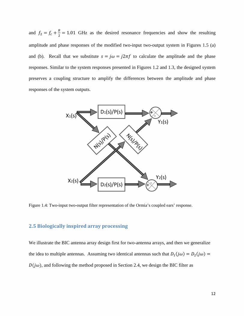
responses of different ears. Using (1.4), we interpret, in Figure 1.4, the mechanical coupling as a
two-input two-output filter that amplifies the differences between the responses of the Ormia’s
ears as shown in Figures 1.2 and 1.3. Inspired by this interpretation, we build a biologically
inspired coupling (BIC) filter first for two-antenna and then for multiple-antenna arrays. In the
following, we show that BIC filter generates a virtual array with a larger aperture, and hence
improves the DOA estimation and radiation performance of an antenna array.
2.4 BIC array response design
We modify the two-input two-output system representing the Ormia’s ears’ responses illustrated
in Figure 1.4 to fit the frequency response of the modified system into the range of desired radio
frequencies. We achieve this conversion by re-assigning the poles of the transfer function
computed in (1.3); that is, we choose the roots of the characteristic function 𝑃𝑃(𝑠𝑠) =
𝐷𝐷1(𝑠𝑠)𝐷𝐷2(𝑠𝑠) −𝑁𝑁2(𝑠𝑠) for frequencies of interest. Characteristic function has 4 complex roots
with imaginary parts representing the resonance frequencies, 𝜋𝜋1 and 𝜋𝜋2 of the system. We change
values of the mass, spring and dash-pot parameters as defined in the analogous mechanical
system to shift these resonance frequencies to fit in the range of the frequencies that we desire
the antenna array to operate. We keep the real parts of the roots as free variables, and later in
Section 2.9, we illustrate how to use these variables to optimize the BIC filter.

11
(a)
(b)
Figure 1.3: Phase responses of the Ormia ochracea’s two ears. (a) Coupled system. (b) Uncoupled system.
For illustrative purposes, assuming a two-antenna array for a narrowband incoming signal with
carrier frequency 𝜋𝜋𝑑𝑑 = 1 GHz and bandwidth 𝐵𝐵 = 20 MHz, we choose 𝜋𝜋1 = 𝜋𝜋𝑑𝑑 −𝐵𝐵2
= 0.99 GHz
12
and 𝜋𝜋2 = 𝜋𝜋𝑑𝑑 + 𝐵𝐵2
= 1.01 GHz as the desired resonance frequencies and show the resulting
amplitude and phase responses of the modified two-input two-output system in Figures 1.5 (a)
and (b). Recall that we substitute 𝑠𝑠 = 𝑗𝑗𝑗𝑗 = 𝑗𝑗2𝜋𝜋𝜋𝜋 to calculate the amplitude and the phase
responses. Similar to the system responses presented in Figures 1.2 and 1.3, the designed system
preserves a coupling structure to amplify the differences between the amplitude and phase
responses of the system outputs.
Figure 1.4: Two-input two-output filter representation of the Ormia’s coupled ears’ response.
2.5 Biologically inspired array processing
We illustrate the BIC antenna array design first for two-antenna arrays, and then we generalize
the idea to multiple antennas. Assuming two identical antennas such that 𝐷𝐷1(𝑗𝑗𝑗𝑗) = 𝐷𝐷2(𝑗𝑗𝑗𝑗) =
𝐷𝐷(𝑗𝑗𝑗𝑗), and following the method proposed in Section 2.4, we design the BIC filter as

13
(a)
(b)
Figure 1.5: (a) Amplitude and (b) phase responses of the converted system.
𝑯𝑯𝐼𝐼(𝑗𝑗𝑗𝑗) = �𝐷𝐷(𝑗𝑗𝑗𝑗) 𝑁𝑁(𝑗𝑗𝑗𝑗)
𝑁𝑁(𝑗𝑗𝑗𝑗) 𝐷𝐷(𝑗𝑗𝑗𝑗)�−1
[1.5]

14
Note here that we substitute 𝑠𝑠 = 𝑗𝑗𝑗𝑗 = 𝑗𝑗2𝜋𝜋𝜋𝜋 to compute the frequency response of the filter from
its system response. Then, applying this filter to the output of (1.1), in the frequency domain we
obtain
�𝑌𝑌1(𝑗𝑗𝑗𝑗)𝑌𝑌2(𝑗𝑗𝑗𝑗)� = 𝑯𝑯𝐼𝐼(𝑗𝑗𝑗𝑗) �
𝑋𝑋1(𝑗𝑗𝑗𝑗)𝑋𝑋2(𝑗𝑗𝑗𝑗)� [1.6]
We assume that the incoming bandlimited signal is narrowband such that inter-element spacing
is much smaller than the reciprocal of the signal bandwidth (Dogandzic & Nehorai 2001). We
further assume that the incoming signal can be approximated as a summation of components
which are almost pure in frequency such that 𝒔𝒔(𝑡𝑡) = ∑ 𝒔𝒔𝑛𝑛𝑁𝑁𝐹𝐹𝑛𝑛=1 (𝑡𝑡), where 𝑁𝑁𝐹𝐹 is the number of
such components. Note that the multiplication in (1.6) corresponds to convolution in time
domain. Due to the narrowband assumption, convolution of the BIC filter with each component
of 𝒔𝒔(𝑡𝑡) results in multiplication of the time domain incoming signal with the BIC filter computed
at the corresponding frequencies of the components (Oppenheim et.al. 1999), (Ottersten et.al.
1993) , (Krim & Viberg 1996). Then under the above mentioned assumptions, we approximate
the output of the BIC filter (1.6) to the 𝑛𝑛𝑡𝑡ℎ component as
𝒚𝒚𝑛𝑛(𝑡𝑡) = �𝑦𝑦1(𝑡𝑡)𝑦𝑦2(𝑡𝑡)�
𝑛𝑛= 𝑯𝑯𝐼𝐼(𝑗𝑗𝑗𝑗𝑛𝑛)𝑨𝑨𝑛𝑛(𝝓𝝓)𝒔𝒔𝑛𝑛(𝑡𝑡) + 𝒆𝒆�𝑛𝑛(𝑡𝑡), 𝑡𝑡 = 1, … ,𝑇𝑇 [1.7]
where 𝒆𝒆�𝑛𝑛(𝑡𝑡) = 𝒆𝒆𝑎𝑎𝑛𝑛(𝑡𝑡) + 𝑯𝑯𝐼𝐼(𝑗𝑗𝑗𝑗𝑛𝑛)𝒆𝒆𝑒𝑒𝑛𝑛(𝑡𝑡), such that only the environment noise is affected by the
BIC filter. Here 𝒆𝒆𝑎𝑎𝑛𝑛(𝑡𝑡) and 𝒆𝒆𝑒𝑒𝑛𝑛(𝑡𝑡) are the amplifier and environment noise components,
respectively, and 𝑗𝑗𝑓𝑓 is the frequency of the component 𝒔𝒔𝑛𝑛(𝑡𝑡). We collect the responses
corresponding to all the components of 𝒔𝒔(𝑡𝑡) as

15
𝒚𝒚(𝑡𝑡) = �𝒚𝒚1…𝒚𝒚𝑁𝑁𝐹𝐹
� = 𝑯𝑯𝐼𝐼𝑨𝑨(𝝓𝝓) 𝒔𝒔�(𝑡𝑡) + 𝒆𝒆�(𝑡𝑡) [1.8]
where
• 𝑯𝑯𝐼𝐼 = blkdiag (𝑯𝑯𝐼𝐼(𝑗𝑗 𝑗𝑗1), … ,𝑯𝑯𝐼𝐼(𝑗𝑗𝑗𝑗𝑁𝑁𝐹𝐹)) is 2𝑁𝑁𝐹𝐹 × 2𝑁𝑁𝐹𝐹 block diagonal matrix with
𝑯𝑯𝐼𝐼(𝑗𝑗𝑗𝑗𝑛𝑛) as the 𝑛𝑛𝑡𝑡ℎ block diagonal entry.
• 𝑨𝑨(𝝓𝝓) = blkdiag (𝑨𝑨1(𝝓𝝓), … ,𝑨𝑨𝑁𝑁𝐹𝐹(𝝓𝝓))
• 𝒔𝒔�(𝑡𝑡) = ��𝒔𝒔1(𝑡𝑡)�𝐿𝐿
, … , �𝒔𝒔𝑁𝑁𝐹𝐹(𝑡𝑡)�𝐿𝐿
� , and
• 𝒆𝒆�(𝑡𝑡) = ��𝒆𝒆�1(𝑡𝑡)�𝐿𝐿
, … , �𝒆𝒆�𝑁𝑁𝐹𝐹(𝑡𝑡)�𝐿𝐿� .
We next extend the model in (1.8) to 𝑀𝑀 identical antennas. We assume that each antenna is
coupled to its immediate neighboring antennas in the array, i.e., each antenna (except for the first
and the last antennas) is coupled to two antennas. Other array structures may also be possible;
however, we focus on the linear arrays which are the most commonly used structures in antenna
array processing. Consequently, for a linear antenna array with 𝑀𝑀 identical antennas, we extend
𝑯𝑯𝐼𝐼(𝑗𝑗𝑗𝑗) defined in (1.6) to an 𝑀𝑀 × 𝑀𝑀 tridiagonal form as
𝑯𝑯𝐼𝐼(𝑗𝑗𝑗𝑗)−1 = �
𝐷𝐷(𝑗𝑗𝑗𝑗) 𝑁𝑁(𝑗𝑗𝑗𝑗) 0 … … 0𝑁𝑁(𝑗𝑗𝑗𝑗)…
0
𝐷𝐷(𝑗𝑗𝑗𝑗)……
𝑁𝑁(𝑗𝑗𝑗𝑗) 0 … 0… … … …
… 0 𝑁𝑁(𝑗𝑗𝑗𝑗) 𝐷𝐷(𝑗𝑗𝑗𝑗)� [1.9]
2.6 Statistical assumptions
We assume in (1.1) that
• 𝝓𝝓 = �𝜙𝜙1, … ,𝜙𝜙𝑄𝑄�𝐿𝐿 is the 𝑄𝑄 × 1 vector of deterministic unknown DOA parameters

16
• 𝒔𝒔�(𝑡𝑡) is a Gaussian input signal vector, 𝐸𝐸[𝒔𝒔�(𝑡𝑡)] = 𝟎𝟎, 𝐸𝐸[𝒔𝒔�(𝑡𝑡)𝒔𝒔�(𝑡𝑡′)𝐻𝐻] = 𝑷𝑷δtt′ and
𝐸𝐸[𝒔𝒔�(𝑡𝑡)𝒔𝒔�(𝑡𝑡′)𝐻𝐻] = 𝟎𝟎 with 𝑷𝑷 as the 𝑄𝑄𝑁𝑁𝐹𝐹 × 𝑄𝑄𝑁𝑁𝐹𝐹 unknown source covariance matrix, and for
𝑡𝑡, 𝑡𝑡′ = 1, … ,𝑇𝑇, 𝛿𝛿𝑡𝑡𝑡𝑡′ = 1 when 𝑡𝑡 = 𝑡𝑡′and zero otherwise
• 𝒆𝒆�(𝑡𝑡) is Gaussian distributed and 𝐸𝐸[𝒆𝒆�(𝑡𝑡)] = 𝟎𝟎 , 𝐸𝐸[𝒆𝒆�(𝑡𝑡)𝒆𝒆�(𝑡𝑡′)𝐻𝐻] = (𝜎𝜎𝑎𝑎2𝑰𝑰 + 𝜎𝜎𝑒𝑒2𝑯𝑯𝐼𝐼𝑯𝑯𝐼𝐼𝐻𝐻)𝛿𝛿𝑡𝑡𝑡𝑡′
and 𝐸𝐸[𝒆𝒆�(𝑡𝑡)𝒆𝒆�(𝑡𝑡′)𝐿𝐿] = 𝟎𝟎, such that 𝜎𝜎𝑎𝑎2 and 𝜎𝜎𝑒𝑒2 are the unknown variances of amplifier and
environment noise, respectively, and
• 𝒔𝒔�(𝑡𝑡) and 𝒆𝒆�(𝑡𝑡′) are uncorrelated for all 𝑡𝑡 and 𝑡𝑡′.
2.7 Maximum likelihood estimation
The maximum likelihood estimate (MLE) of the DOA is defined as the value that maximizes the
likelihood function (see (1.11)). It is asymptotically unbiased and it attains the Cramér-Rao
bound (CRB) of minimum variance (Kay 1993). In the following, we demonstrate the derivation
of the MLE of DOA, and in Section 2.8, we compute the CRB on DOA estimation. First,
following the statistical assumptions in Section 2.6, we write the probability density function of
the measurements 𝒚𝒚(𝑡𝑡) as
∏ 𝑝𝑝[𝒚𝒚(𝑡𝑡);𝝓𝝓,𝑷𝑷,𝜎𝜎𝑎𝑎2,𝜎𝜎𝑒𝑒2] = ∏ 1|𝜋𝜋𝑹𝑹| exp[𝒚𝒚(𝑡𝑡)𝐻𝐻𝑹𝑹−1𝒚𝒚(𝑡𝑡)]𝐿𝐿
𝑡𝑡=1𝐿𝐿𝑡𝑡=1 [1.10]
where 𝑹𝑹 = 𝐸𝐸[𝒚𝒚(𝑡𝑡)𝒚𝒚(𝑡𝑡)𝐻𝐻] = 𝑨𝑨�(𝝓𝝓)𝑷𝑷 𝑨𝑨�(𝝓𝝓)𝐻𝐻 + 𝜎𝜎𝑒𝑒2𝚺𝚺(𝜌𝜌), with 𝚺𝚺(𝜌𝜌) = 𝜌𝜌𝑰𝑰 + 𝑯𝑯𝐼𝐼𝑯𝑯𝐼𝐼𝐻𝐻, 𝜌𝜌 = 𝜎𝜎𝑎𝑎2/𝜎𝜎𝑒𝑒2,
and 𝑨𝑨�(𝝓𝝓) = 𝑯𝑯𝐼𝐼𝑨𝑨(𝝓𝝓). To whiten the noise, we compute 𝚺𝚺(𝜌𝜌)−1/2 , and define 𝒚𝒚 �(𝑡𝑡) =
𝚺𝚺(𝜌𝜌)−12𝒚𝒚(𝑡𝑡) and 𝑨𝑨�(𝜽𝜽) = 𝚺𝚺(𝜌𝜌)−1/2 𝑨𝑨� (𝝓𝝓) where 𝜽𝜽 = [𝜌𝜌,𝝓𝝓]𝐿𝐿is (𝑄𝑄 + 1) × 1 vector of unknown
parameters including the DOA, 𝝓𝝓. Accordingly, the joint distribution of 𝒚𝒚 �(𝑡𝑡) for 𝑡𝑡 = 1, … ,𝑇𝑇
is

17
∏ 𝑝𝑝[𝒚𝒚�(𝑡𝑡);𝜙𝜙,𝜌𝜌,𝑷𝑷,𝜎𝜎𝑒𝑒2]𝐿𝐿𝑡𝑡=1 = ∏ 1
�𝜋𝜋 𝑹𝑹� � exp�𝒚𝒚�(𝑡𝑡)𝐻𝐻 𝑹𝑹�−1 𝒚𝒚� (𝑡𝑡)�𝐿𝐿
𝑡𝑡=1 [1.11]
where 𝑹𝑹� = 𝐸𝐸[𝒚𝒚� (𝑡𝑡)𝒚𝒚�(𝑡𝑡)𝐻𝐻] = 𝑨𝑨�(𝜽𝜽)𝑷𝑷𝑨𝑨�(𝜽𝜽)𝐻𝐻 + 𝜎𝜎𝑒𝑒2𝑰𝑰 . We, then, follow the procedure explained in
(Stoica & Nehorai 1995), first using (1.11), we derive the MLEs of 𝑷𝑷 and 𝝈𝝈𝑒𝑒2 as a function of the
unknown parameter vector 𝜽𝜽, denoted by 𝑷𝑷�(𝜽𝜽) and 𝜎𝜎�𝑒𝑒2(𝜽𝜽), respectively. We then concentrate
the likelihood in (1.11) using these MLEs, and accordingly find the MLE of 𝜽𝜽 by solving the
following optimization problem
𝜽𝜽� = argmin𝜃𝜃 ln�𝑨𝑨�(𝜽𝜽)𝑷𝑷�(𝜽𝜽)𝑨𝑨�(𝜽𝜽)𝐻𝐻 + 𝜎𝜎�𝑒𝑒2(𝜽𝜽)𝑰𝑰� [1.12]
where
• 𝑷𝑷�(𝜽𝜽) = 𝑨𝑨�(𝜽𝜽)ϯ 𝑹𝑹 � �𝑨𝑨�(𝜽𝜽)ϯ�𝐻𝐻− 𝜎𝜎�𝑒𝑒2(𝜽𝜽)(𝑨𝑨�(𝜽𝜽)𝑨𝑨�(𝜽𝜽)𝐻𝐻)−1 is the MLE of 𝑷𝑷 as a function of 𝜽𝜽
• 𝜎𝜎�𝑒𝑒2(𝜽𝜽) = tr�𝚷𝚷⊥ 𝑹𝑹� �𝑴𝑴−𝑸𝑸
is the MLE of 𝜎𝜎𝑒𝑒2 as a function of 𝜽𝜽
• 𝑹𝑹� = ∑ 𝒚𝒚�𝐿𝐿𝑡𝑡=1 (𝑡𝑡) 𝒚𝒚�(𝑡𝑡)𝐻𝐻 is the sample covariance
• 𝑨𝑨�(𝜽𝜽)ϯ = [ 𝑨𝑨� (𝜽𝜽)𝐻𝐻𝑨𝑨�(𝜽𝜽)]−1 𝑨𝑨� (𝜽𝜽)𝐻𝐻
• 𝚷𝚷⊥ = 𝑰𝑰 − 𝑨𝑨�(𝜽𝜽)𝑨𝑨�(𝜽𝜽)ϯ .
2.8 Performance analysis
We analyze the array's statistical performance, i.e., accuracy in estimating the source direction,
by computing the Cramér-Rao bound. The CRB is the lower bound on estimation error for any
unbiased estimator. We concentrate the likelihood function in (1.11) with respect to 𝑷𝑷 and 𝜎𝜎𝑒𝑒2
and compute the CRB on the covariance matrix of any unbiased estimator of 𝜽𝜽. Using the results
in (Stoica & Nehorai 1990) and (Nehorai & Paldi 1994),

18
CRB(𝜽𝜽) = 𝜎𝜎𝑒𝑒2
2𝐿𝐿 �Re�btr �(𝟏𝟏 ⊗𝑼𝑼) ⊡ (𝑫𝑫𝐻𝐻𝚷𝚷⊥𝑫𝑫)bT�� �
−1 [1.13]
where
• 𝟏𝟏 is a 𝑄𝑄 + 1 × 𝑄𝑄 + 1 matrix of ones
• 𝑼𝑼 = 𝑷𝑷 �𝑨𝑨�(𝜽𝜽)𝐻𝐻 𝑨𝑨� (𝜽𝜽)𝑷𝑷 + 𝜎𝜎𝑒𝑒2𝑰𝑰�−1𝑨𝑨�(𝜽𝜽)𝐻𝐻 𝑨𝑨� (𝜽𝜽)𝑷𝑷
• 𝑫𝑫 = �𝑫𝑫1 …𝑫𝑫𝑄𝑄+1 � with 𝑫𝑫𝑖𝑖 = 𝜕𝜕𝑨𝑨� (𝜽𝜽)𝜕𝜕𝜃𝜃𝑖𝑖
• btr and bT are block trace and transpose operators, respectively
• ⊗ is the Kronecker product, and
• ⊡ is the block Schur-Hadamard product.
Note: see Appendix A for the definition of the block matrix operators.
2.9 Optimization of the BIC
In this section, we develop a method to maximize the localization performance of the antenna
array by optimizing the CRB on DOA estimation with respect to the BIC parameters. We first
introduce the optimization parameters, and then formulate a cost function employing the CRB on
DOA estimation for optimum performance. Note here that we optimize the value of the BIC for
the antenna array structures (linear) and coupling configurations (coupling with adjacent
antennas) as discussed in Section 2.5. Other array structures and different coupling
configurations are also possible.
As explained in Section 2.4, to fit the frequency response of the modified BIC system into the
range of desired radio frequencies, we change the imaginary parts of the poles of the
characteristic function to shift the resonance frequencies of the system response while we keep

19
the real parts as free variables. Therefore, under the constraints that we explain below, we have
the freedom of choosing the real parts for optimum coupling design. As defined in (1.2) and
described in Section 2.4, we compute the poles of the system as a function of system parameters
(𝑘𝑘s, 𝑐𝑐s and 𝑚𝑚0). As stated in Section 2.5, we assume identical antennas (𝐷𝐷1(𝑠𝑠) = 𝐷𝐷2(𝑠𝑠) = 𝐷𝐷(𝑠𝑠)
and hence 𝑘𝑘1 = 𝑘𝑘2 = 𝑘𝑘, 𝑐𝑐1 = 𝑐𝑐2 = 𝑐𝑐), and write the characteristic function 𝑃𝑃(𝑠𝑠) as
𝑃𝑃(𝑠𝑠) = 𝐷𝐷(𝑠𝑠)2 − 𝑁𝑁(𝑠𝑠)2 = 𝑚𝑚02[(𝑠𝑠2 + 𝑏𝑏1𝑠𝑠 + 𝑎𝑎1) − (𝑏𝑏2𝑠𝑠 + 𝑎𝑎2)^2] [1.14]
where 𝑎𝑎1 = (𝑘𝑘+𝑘𝑘3)𝑚𝑚0
, 𝑎𝑎2 = 𝑘𝑘3𝑚𝑚0
, 𝑏𝑏1 = (𝑑𝑑+𝑑𝑑3)𝑚𝑚0
, and 𝑏𝑏2 = 𝑑𝑑3𝑚𝑚0
with the assumption that 𝑎𝑎1,𝑎𝑎2, 𝑏𝑏1, and
𝑏𝑏2 are all positive. Then accordingly, we compute the poles of the characteristic function 𝑃𝑃(𝑠𝑠) as
𝑝𝑝1,2 = −𝑟𝑟1 ± �𝑖𝑖1𝑝𝑝3,4 = −𝑟𝑟2 ± �𝑖𝑖2
[1.15]
where 𝑟𝑟1 = 12
(𝑏𝑏1 + 𝑏𝑏2), 𝑟𝑟2 = 12
(𝑏𝑏1 − 𝑏𝑏2), 𝑖𝑖1 = 14
[(𝑏𝑏1 + 𝑏𝑏2)2 − 4(𝑎𝑎1 + 𝑎𝑎2)], and 𝑖𝑖2 =
14
[(𝑏𝑏1 − 𝑏𝑏2)2 − 4(𝑎𝑎1 − 𝑎𝑎2)]. As explained in Section 2.4, to fit the frequency response of the
modified BIC system into the range of desired radio frequencies, we change the imaginary parts
Note here that the real parameters, 𝑟𝑟1and 𝑟𝑟2 are free parameters and we have the freedom to
control them as long as 𝑟𝑟1 > 𝑟𝑟2 due to the positivity assumption on 𝑎𝑎1, 𝑎𝑎2, 𝑏𝑏1, and 𝑏𝑏2. From
(1.9), (1.11), (1.13), (1.14), and (1.15), we observe that CRB is also a function of the real parts of
the poles of the characteristics function. Accordingly, we propose to choose 𝑟𝑟1 and 𝑟𝑟2 by
minimizing the CRB on DOA estimation. This is a reasonable choice since minimizing the CRB
minimizes the lower bound on the error of the MLE of DOA. Defining 𝒓𝒓 = [𝑟𝑟1, 𝑟𝑟2]𝐿𝐿, we design
the optimum BIC by solving the following constrained optimization problem
argmin𝒓𝒓 tr [CRB(𝜽𝜽, 𝒓𝒓)] s. t. r1 − 𝑟𝑟2 > 0 [1.16]

20
where by taking the trace of the CRB(𝜽𝜽, 𝒓𝒓) , we minimize the sum of the variance of the errors on
the DOA, 𝝓𝝓, and noise-to-interference ratio (NIR) estimation. We define the numerical value of
NIR as 𝜌𝜌 = 𝜎𝜎𝑎𝑎2/𝜎𝜎𝑒𝑒2.
3 Biologically inspired coupled antenna beampattern design
In this section, inspired by the female Ormia's coupled ears, we show that applying biologically
inspired coupling amongst antennas is beneficial to achieve high radiation performance. Our goal
is to demonstrate the effect of the BIC on the radiation performance. We would like to note that
our approach, namely employing BIC, might be also used to complement the existing
superdirective (super gain) array design methods that overcome issues; for example, the effect of
the undesired coupling on individual antenna impedance (Tucker 1967), (Newman et.al. 1978),
(Popovic et.al. 1999), (Lee & Wang 2008).
3.1 Biologically inspired coupled array factor
In this section, we compute the array factor of the proposed biologically inspired uniform linear
array (ULA). We start with the array factor of a standard ULA, positioned without loss of
generality along the z-axis (see Figure 1.6). Since we focus on systems confined in small spaces,
we also consider the undesired electromagnetic coupling between the array elements.
Under the far-field radiation and narrow-band signal assumption, we modify the uniform linear
array factor to include the undesired coupling between the elements (see also (Allen & Diamond
1966)):
AF(𝜃𝜃) = ∑ 𝑝𝑝𝑚𝑚 exp�−𝑗𝑗 (𝑚𝑚− 1)(𝑗𝑗Δ + 𝛽𝛽)�𝑀𝑀𝑚𝑚=1 [1.17]

21
Figure 1.6: Far-field radiation geometry of M-element antenna array.
where
• AF(𝜃𝜃) is the radiation pattern (desired amplitude and phase in each direction) of 𝑀𝑀-
element array assuming isotropic antennas, which depends on the positions and
excitations of the sensing elements in the system
• 𝒑𝒑 = [𝑝𝑝1, … ,𝑝𝑝𝑀𝑀]𝐿𝐿 = 𝑪𝑪𝒗𝒗𝑔𝑔 is the vector of the currents on the antennas
• 𝒗𝒗𝑔𝑔 = [𝑣𝑣1, … , 𝑣𝑣𝑀𝑀] is the vector of generator (excitation) voltages at the input of the
antennas
• 𝑪𝑪 is the undesired electromagnetic coupling between the array elements, (a
transformation matrix, transforming generator voltages to the induced currents on each
antenna)
• As also defined earlier, Δ = 𝑑𝑑 cos𝜃𝜃𝑣𝑣
is the inter-element time difference
• 𝜃𝜃 is the elevation angle (see Figure 1.6), and
• 𝛽𝛽 is the excitation phase.

22
We compute 𝑪𝑪 similar to (Allen & Diamond 1966) as a function of self and mutual impedances
between the antennas (see also discussions in (Gupta and Ksienski 1983) and (Svantesson
1998)). We summarize the computation of 𝑪𝑪 in Appendix B. When the mutual impedances are
zero, when there is no electromagnetic coupling, 𝑪𝑪 reduces to a diagonal matrix. We compute the
self and mutual impedances, assuming finite-length dipole antennas as the elements of the array,
as explained in (Balanis 1982, Chapter 8). Note that the standard literature often ignores 𝑪𝑪,
which is reasonable for sufficiently large inter-elemental distances.
The usual goal of the array-factor design is to select the excitation voltages, 𝒗𝒗𝑔𝑔, and phase, 𝛽𝛽, to
obtain a desired radiation pattern. Our goal is to include the BIC in the array factor for fixed
𝒗𝒗𝑔𝑔 and 𝛽𝛽 values and demonstrate the improvement in the directivity gain, half-power beamwidth
(HPBW) and side lobe level (SLL) of the radiation pattern.
Next, we generalize (1.19) to include also the coupling biologically inspired by the Ormia's
coupled ears. We follow the discussions in Sections 2.4 and 2.5 to obtain the frequency
responses of the converted system and generalize (1.17) employing
AFI(𝜃𝜃) = ∑ 𝑝𝑝𝑚𝑚𝑀𝑀𝑚𝑚=1 �𝐻𝐻2(𝑤𝑤,Δ,𝛽𝛽)
𝐻𝐻1(𝜔𝜔,Δ,𝛽𝛽)�𝑚𝑚−1
= ∑ 𝑝𝑝𝑚𝑚𝑀𝑀𝑚𝑚=1 �𝐷𝐷(𝑗𝑗𝜔𝜔)exp�−𝑗𝑗 (𝜔𝜔Δ+𝛽𝛽)�−𝑁𝑁(𝑗𝑗𝜔𝜔)
𝐷𝐷(𝑗𝑗𝜔𝜔)−𝑁𝑁(𝑗𝑗𝜔𝜔)exp�−𝑗𝑗 (𝜔𝜔Δ+𝛽𝛽)��𝑚𝑚−1
[1.18]
where 𝐻𝐻2(𝑤𝑤,Δ,𝛽𝛽)𝐻𝐻1(𝜔𝜔,Δ,𝛽𝛽) is the ratio between the responses of two consecutive antennas in the BIC
antenna array. These responses follow the same structure as the responses of Ormia’s ears as
defined in (1.4), but operate in a different frequency range. This ratio generalizes the exponential
terms in (1.17) to include the BIC between antennas. In this setup, every antenna is coupled with
its immediate neighbor antennas. In (1.18), we also assume identical antennas such that

23
𝐷𝐷1(𝑗𝑗𝑗𝑗) = 𝐷𝐷2(𝑗𝑗𝑗𝑗) = 𝐷𝐷(𝑗𝑗𝑗𝑗). Note here that 𝑁𝑁(𝑗𝑗𝑗𝑗) represents the BIC and when there is no
coupling (𝑁𝑁(𝑗𝑗𝑗𝑗) = 0), AFI(𝜃𝜃) reduces to AF(𝜃𝜃).
3.2 Performance measures
In this section, we describe our measures that we employ to analyze the radiation performance.
First, taking into account the antenna factor (element factor) and the BIC, we compute the
radiation intensity of the antenna array in a given direction (Balanis 1982)
𝑈𝑈𝐼𝐼(𝜃𝜃,𝜙𝜙) = [EF(𝜃𝜃,𝜙𝜙)]𝑛𝑛2[AFI(𝜃𝜃)]𝑛𝑛2 [1.19]
where
• [EF(𝜃𝜃,𝜙𝜙)]𝑛𝑛2 is the normalized element factor, far-zone electric field of a single element
(in our work we assume that the array is formed with finite-length dipoles, see also
Section 4.2 )
• [AFI(𝜃𝜃)]𝑛𝑛2 is the normalized array factor, and
• 𝑈𝑈𝐼𝐼(𝜃𝜃,𝜙𝜙), the radiation intensity in a given direction, is the power radiated from an
antenna array per unit solid angle.
Hence the radiated power 𝑃𝑃rad is
𝑃𝑃rad = = ∫ ∫ 𝑈𝑈𝐼𝐼(𝜃𝜃,𝜙𝜙) sin𝜃𝜃 d𝜃𝜃 d𝜙𝜙𝜋𝜋0
2𝜋𝜋0 [1.20]
where 𝜃𝜃 and 𝜙𝜙 are the elevation and azimuth angles, respectively, and sin𝜃𝜃 d𝜃𝜃 d𝜙𝜙 is the unit
solid angle.
Using the radiation intensity, we consider the following measures to analyze the performance of
the beampattern design:

24
• Directivity, 𝐷𝐷𝐼𝐼(𝜃𝜃,𝜙𝜙), is the ratio of the radiation intensity in a given direction to the
average radiation intensity
𝐷𝐷𝐼𝐼(𝜃𝜃,𝜙𝜙) = 4𝜋𝜋𝑈𝑈𝐼𝐼(𝜃𝜃,𝜙𝜙)𝑃𝑃rad
[1.21]
where 𝑃𝑃rad4𝜋𝜋
is the average radiation intensity over all angles. In our work, for comparison
purposes, we consider the directivity gain in a desired direction.
• Half-power beamwidth, HPBW, in terms of the elevation angle, 𝜃𝜃, for a fixed azimuth
angle, 𝜙𝜙. HPBW is defined as the angle between two half-power directions (Balanis
1982).
• Sidelobe level (SLL) defined as the maximum value of the radiation pattern in any
direction other than the desired one.
The directivity gain, HPBW and SLL measure how effectively the power is directed (steered) in
a given direction. For a good performance, it is desirable to have large 𝐷𝐷𝐼𝐼(𝜃𝜃,𝜙𝜙), small SLL and
narrow HPBW in a desired direction.
3.3 Optimization of the BIC
In this section, we develop a method to maximize the radiation performance by optimizing the
BIC. We formulate the optimization problem to improve the radiation performance. For an
antenna array, we choose the directivity gain in a desired direction as the utility function to be
maximized. This is a reasonable choice since the directivity gain is also related to the SLL and
the HPBW of the radiation pattern. Generally it is true that the patterns with smaller SLL and
HPBW values have larger directivity gain. Following the discussions from Section 2.9, using
equations (1.4), (1.14), (1.15), (1.18), (1.19), (1.20), and (1.21), we observe that directivity is

25
also a function of the real parts of the poles of the characteristics function. Accordingly, to
optimize the BIC for maximum directivity, we propose to choose 𝑟𝑟1 and 𝑟𝑟2 by solving the
following constrained optimization problem in the desired direction of transmission with
elevation 𝜃𝜃 and azimuth 𝜙𝜙
max𝒓𝒓 𝐷𝐷𝐼𝐼(𝜃𝜃,𝜙𝜙, 𝒓𝒓) s. t. 𝑟𝑟1 − 𝑟𝑟2 > 0 [1.22]
4 Numerical results
In this section, we present numerical simulation results for the comparison of radiation and
localization performances of biologically inspired coupled and standard antenna arrays. In the
following, by BIC and standard arrays we refer to the systems with and without the BIC.
4.1 BIC antenna array for DOA estimation
We compare the localization performances of the BIC and standard multiple-antenna arrays
using Monte Carlo simulations. In these examples, we focus on the optimally designed BIC as
described in Section 2.9. We follow the statistical assumptions stated in Section 2.6.
We compare the BIC array with the multi-channel cross-correlation method. Under our statistical
assumptions multi-channel cross-correlation method asymptotically reduces to the ML
estimation of DOA using a standard antenna array (Chen et.al. 2003). Therefore for comparison,
we demonstrate the results of the ML estimation of the DOA and compute the corresponding
CRB using the standard antenna array and the antenna array with BIC. We focus on the small-
sized compact arrays that are very important for civil and military purposes to be used in tactical

26
and mobile applications which are confined in small spaces. We use the following scenarios for
the multiple-antenna array.
• Uniform Linear Array (ULA): 5 identical dipole antennas, 𝑑𝑑 = 0.1𝜆𝜆 and 𝑑𝑑 = 0.2 inter-
element distances
• 𝜋𝜋𝑑𝑑 = 1GHz is the carrier frequency; 𝜋𝜋1 = 0.99 GHz and 𝜋𝜋2 = 1.1 GHz are the resonant
frequencies which are employed as in Section 2.4; 𝜌𝜌 = 𝜎𝜎𝑎𝑎2/𝜎𝜎𝑒𝑒2 is the NIR as defined in
Section 2.9; signal-to-noise ratio is SNR = tr �𝑨𝑨 � (𝝓𝝓)𝑷𝑷𝑷 𝑨𝑨�𝐻𝐻(𝝓𝝓)�𝜎𝜎𝑒𝑒2tr[𝚺𝚺(ρ)] ; root mean-square-error is
RMSE = � 1MC
∑ �𝜙𝜙�𝑖𝑖 − 𝜙𝜙0�2MC
𝑖𝑖=1 where MC is the number of Monte Carlo simulations, 𝜙𝜙0
is the true value of the DOA, and 𝜙𝜙�𝑖𝑖 is the estimate of DOA at the 𝑖𝑖𝑡𝑡ℎ simulation; and
MC =1000.
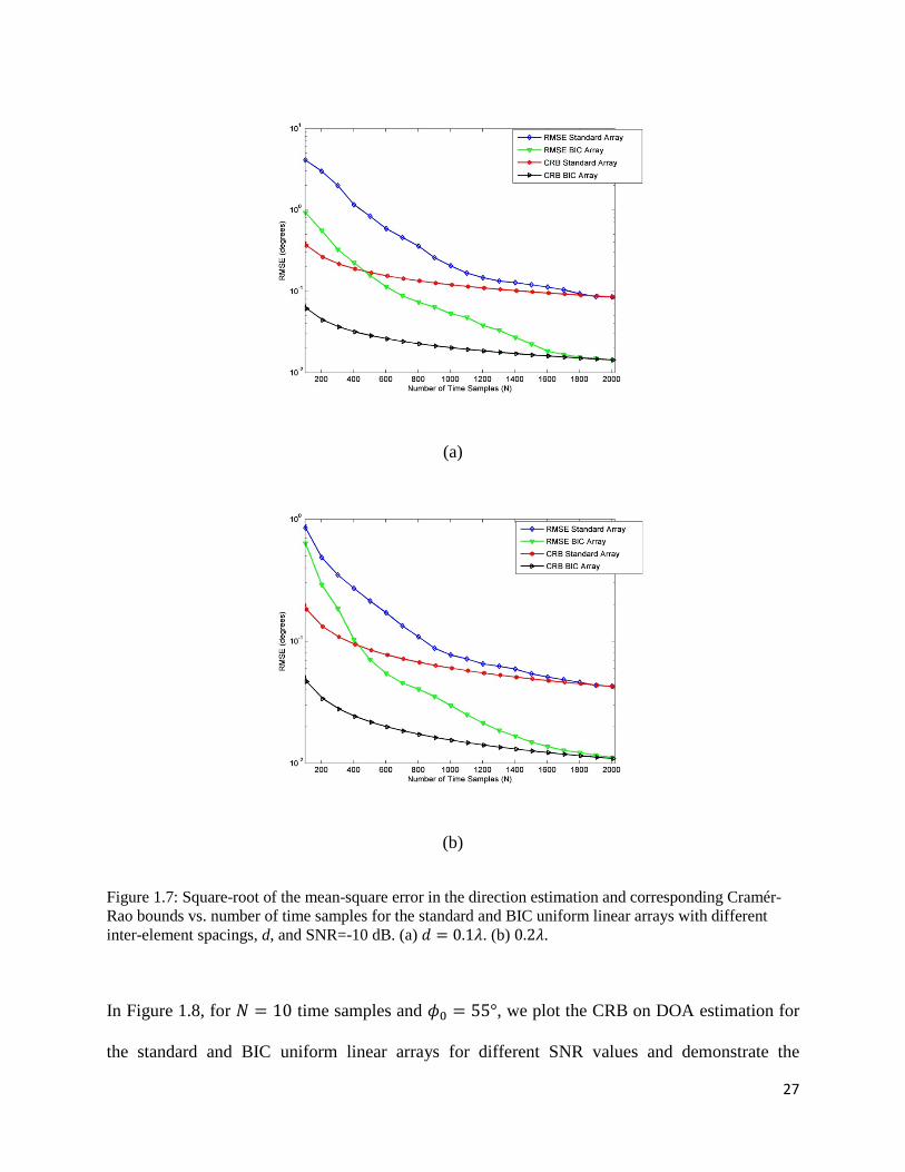
We demonstrate our results on direction of arrival estimation performance in Figures 1.7, 1.8,
1.9, 1.10 and 1.11. In Figures 1.7 (a) and 1.7 (b) for a fixed SNR=-10 dB and the true value of
the azimuth of DOA, 𝜙𝜙0 = 55°, we plot the RMSE for the maximum likelihood estimation of
DOA, and CRB of DOA estimation for the standard and BIC arrays with 𝑑𝑑 = 0.1𝜆𝜆 and 𝑑𝑑 = 0.2𝜆𝜆
inter-element spacings, respectively. Since BIC creates a virtual array with larger aperture, we
observe that the CRB on DOA estimation error and RMSE of MLE are smaller for the BIC array,
meaning a decrease in estimation error and an improvement in the localization performance.
Moreover the MLE algorithm attains the bound asymptotically. BIC array outperforms the
standard array in ML estimation of DOA accuracy. Therefore asymptotically BIC array is better
than the multi-channel cross-correlation method, which is asymptotically the ML estimation of
DOA using standard array.
27
(a)
(b)
Figure 1.7: Square-root of the mean-square error in the direction estimation and corresponding Cramér-Rao bounds vs. number of time samples for the standard and BIC uniform linear arrays with different inter-element spacings, d, and SNR=-10 dB. (a) 𝑑𝑑 = 0.1𝜆𝜆. (b) 0.2𝜆𝜆.
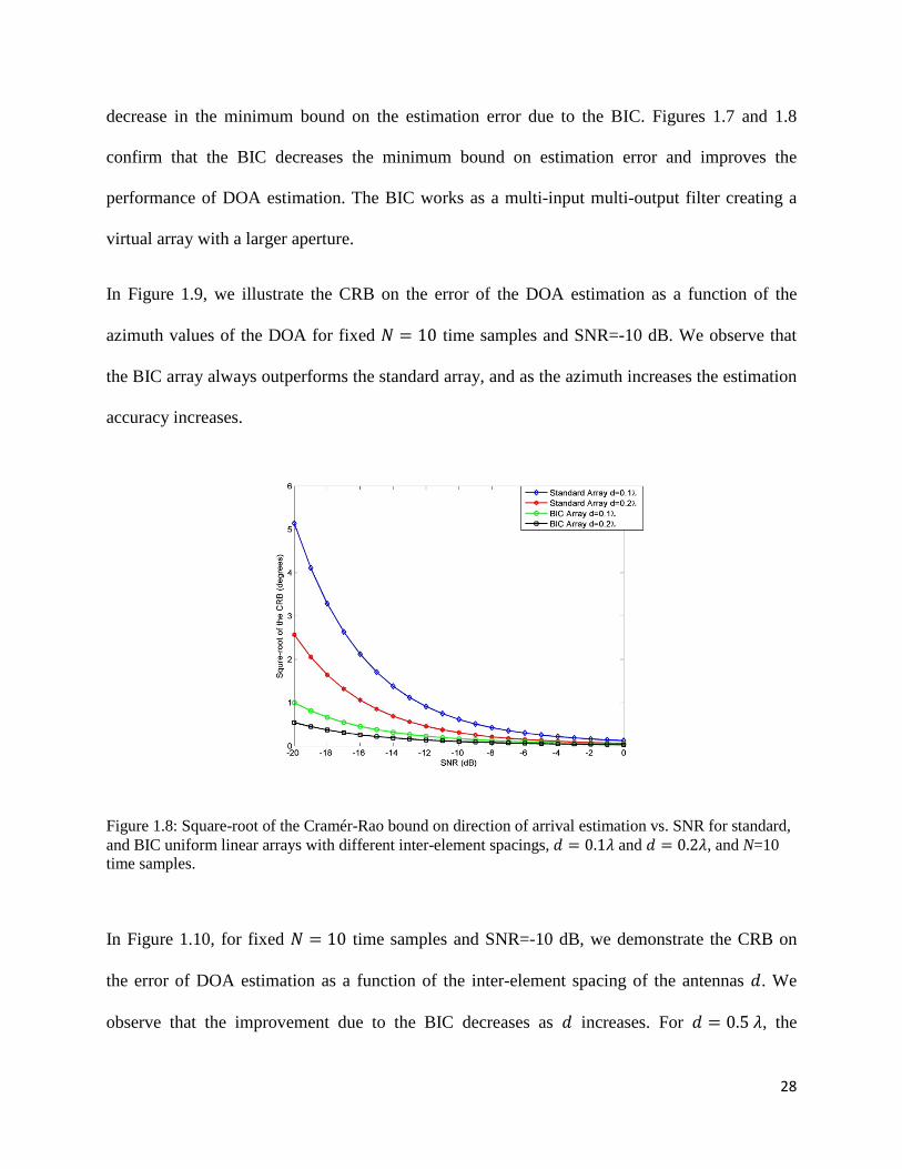
In Figure 1.8, for 𝑁𝑁 = 10 time samples and 𝜙𝜙0 = 55°, we plot the CRB on DOA estimation for
the standard and BIC uniform linear arrays for different SNR values and demonstrate the
28
decrease in the minimum bound on the estimation error due to the BIC. Figures 1.7 and 1.8
confirm that the BIC decreases the minimum bound on estimation error and improves the
performance of DOA estimation. The BIC works as a multi-input multi-output filter creating a
virtual array with a larger aperture.
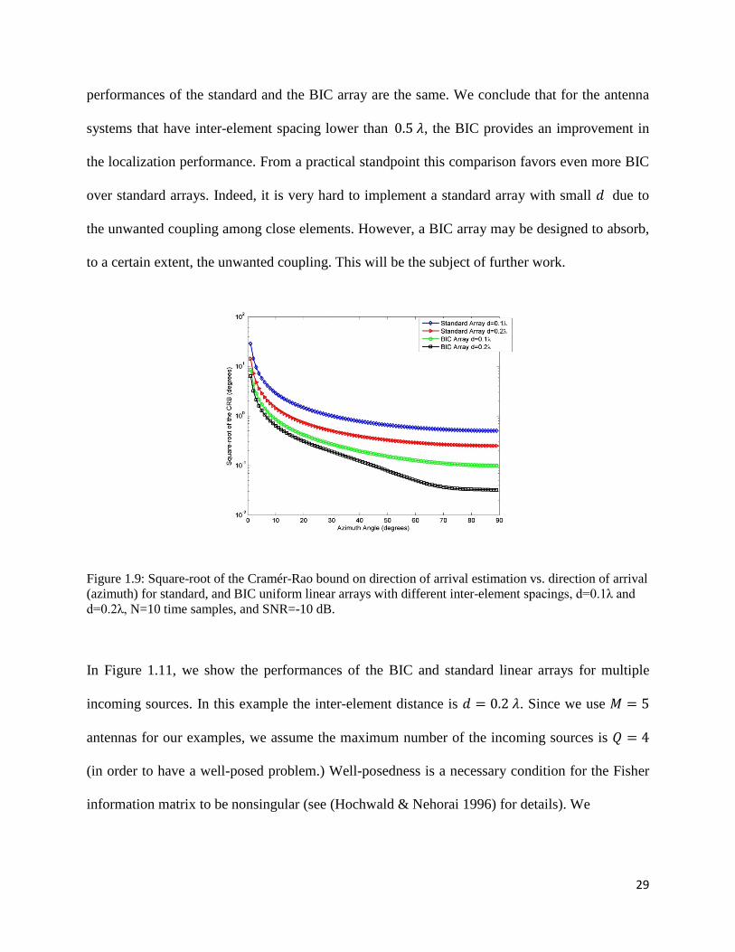
In Figure 1.9, we illustrate the CRB on the error of the DOA estimation as a function of the
azimuth values of the DOA for fixed 𝑁𝑁 = 10 time samples and SNR=-10 dB. We observe that
the BIC array always outperforms the standard array, and as the azimuth increases the estimation
accuracy increases.
Figure 1.8: Square-root of the Cramér-Rao bound on direction of arrival estimation vs. SNR for standard, and BIC uniform linear arrays with different inter-element spacings, 𝑑𝑑 = 0.1𝜆𝜆 and 𝑑𝑑 = 0.2𝜆𝜆, and N=10 time samples.
In Figure 1.10, for fixed 𝑁𝑁 = 10 time samples and SNR=-10 dB, we demonstrate the CRB on
the error of DOA estimation as a function of the inter-element spacing of the antennas 𝑑𝑑. We
observe that the improvement due to the BIC decreases as 𝑑𝑑 increases. For 𝑑𝑑 = 0.5 𝜆𝜆, the
29
performances of the standard and the BIC array are the same. We conclude that for the antenna
systems that have inter-element spacing lower than 0.5 𝜆𝜆, the BIC provides an improvement in
the localization performance. From a practical standpoint this comparison favors even more BIC
over standard arrays. Indeed, it is very hard to implement a standard array with small 𝑑𝑑 due to
the unwanted coupling among close elements. However, a BIC array may be designed to absorb,
to a certain extent, the unwanted coupling. This will be the subject of further work.
Figure 1.9: Square-root of the Cramér-Rao bound on direction of arrival estimation vs. direction of arrival (azimuth) for standard, and BIC uniform linear arrays with different inter-element spacings, d=0.1λ and d=0.2λ, N=10 time samples, and SNR=-10 dB.
In Figure 1.11, we show the performances of the BIC and standard linear arrays for multiple
incoming sources. In this example the inter-element distance is 𝑑𝑑 = 0.2 𝜆𝜆. Since we use 𝑀𝑀 = 5
antennas for our examples, we assume the maximum number of the incoming sources is 𝑄𝑄 = 4
(in order to have a well-posed problem.) Well-posedness is a necessary condition for the Fisher
information matrix to be nonsingular (see (Hochwald & Nehorai 1996) for details). We

30
choose 55°, 10°, 45° and 85° as the azimuths of the true DOA of the incoming sources 1, 2, 3
and 4, respectively. In this figure, we plot the CRB on the estimation of the DOA of the first
source as a function of the SNR in the presence of other sources. For 𝑄𝑄 = 2, we use the sources
1 and 2, for 𝑄𝑄 = 3, we use sources 1,2 and 3 etc. We observe that the BIC array has better
localization performance than the standard array in the presence of multiple sources.
Figure 1.10: Square-root of the Cramér-Rao bound on direction of arrival estimation vs. inter-element spacing, 𝑑𝑑, for standard, and BIC uniform linear arrays, N=10 time samples, and SNR=-10 dB.
4.2 BIC for antenna beampattern design
In this section, we compare the radiation performances of the BIC and standard antenna arrays.
For comparison, we plot the radiation pattern and compare the directivity gain, half-power
beamwidths and sidelobe attenuation of these systems. BIC parameters are optimally designed
using the algorithm described in Section 3.3. We use the following system setup for illustration
purposes.

31
(a)
(b)
Figure 1.11: Square-root of the Cramér-Rao bound on direction of arrival estimation vs. SNR for standard, and BIC uniform linear arrays with different number of sources, 𝑄𝑄, N=10 time samples. (a) 𝑄𝑄 = 2, 3. (b) 𝑄𝑄 = 4.

32
• We consider uniform (uniform excitation voltages) ordinary and binomial (binomial
expansion coefficients as the excitation voltage values) end-fire arrays with 20 identical
dipole antennas (Balanis 1982, Chapter 8), maximum at 𝜃𝜃 = 0° and 𝛽𝛽 = −𝑤𝑤Δ.
• We assume the radiation frequency is 𝜋𝜋 = 1GHz.
• The undesired coupling matrices, 𝑪𝑪 for 0.5𝜆𝜆-wavelength antenna system with different
inter-element distances (𝑑𝑑 = 0.25𝜆𝜆 and 𝑑𝑑 = 0.1𝜆𝜆) are calculated according to (Balanis
1982) for finite-length thin-dipole antennas.
• The antennas are located on the z-axis parallel to y-axis, then assuming azimuth 𝜙𝜙 = 90°
(on the y-z plane, see Figure 1.6), we compute the element factor for a finite-length
dipole antenna as 𝐸𝐸𝐸𝐸 (𝜃𝜃, 90°) = �cos�𝑘𝑘𝑘𝑘2 sin𝜃𝜃�−cos�
𝑘𝑘𝑘𝑘2 �
cos𝜃𝜃� with 𝑘𝑘 = 2 𝜋𝜋
𝜆𝜆, 𝜆𝜆 as the wavelength
of the radiated signal, and 𝑙𝑙 as the length of each antenna.
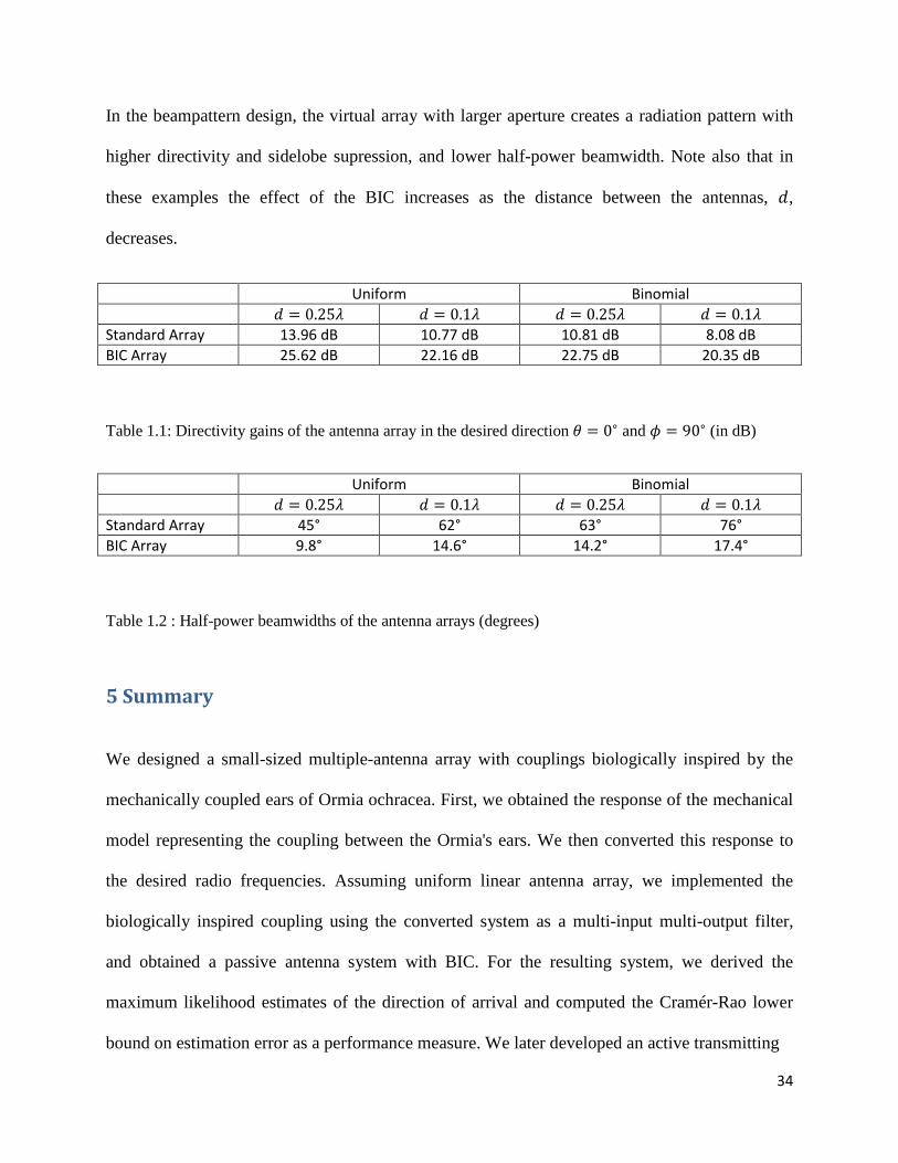
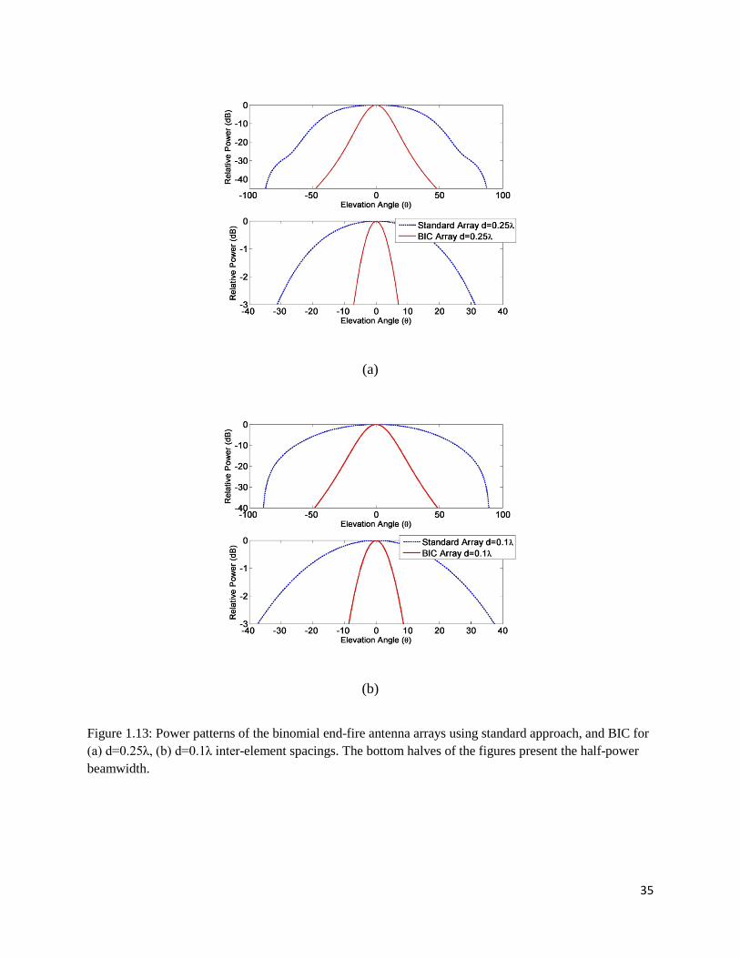
We demonstrate our results in Figures 1.12 and 1.13, and summarize the calculated directivity
gains, and HPBW values in Tables 1.1 and 1.2, respectively. We observe that the BIC array with
uniform excitation voltages outperforms the uniform standard array in terms of sidelobe
suppression, directivity, and HPBW (see Figure 1.12, and Tables 1.1 and 1.2). For binomial
array, in Figure 1.13, we observe that neither the standard nor the BIC array have sidelobes, but
the BIC array has much narrower HPBW and hence better directivity gain (see also Tables 1.1
and 1.2). The physical reason of the improvement in the radiation performance is the BIC that
works as a multi-input multi-output filter, magnifying the amplitude and phase differences (time
differences) between the outputs of the successive antennas and creating a virtual array with a
larger aperture.

33
(a)
(b)
Figure 1.12: Power patterns of the uniform ordinary end-fire antenna arrays using standard approach, and BIC for (a) 𝑑𝑑 = 0.25𝜆𝜆, (b) 𝑑𝑑 = 0.1𝜆𝜆 inter-element spacings. The bottom halves of the figures present the half-power beamwidth.
34
In the beampattern design, the virtual array with larger aperture creates a radiation pattern with
higher directivity and sidelobe supression, and lower half-power beamwidth. Note also that in
these examples the effect of the BIC increases as the distance between the antennas, 𝑑𝑑,
decreases.
Uniform Binomial 𝑑𝑑 = 0.25𝜆𝜆 𝑑𝑑 = 0.1𝜆𝜆 𝑑𝑑 = 0.25𝜆𝜆 𝑑𝑑 = 0.1𝜆𝜆 Standard Array 13.96 dB 10.77 dB 10.81 dB 8.08 dB BIC Array 25.62 dB 22.16 dB 22.75 dB 20.35 dB
Table 1.1: Directivity gains of the antenna array in the desired direction 𝜃𝜃 = 0∘ and 𝜙𝜙 = 90∘ (in dB)
Uniform Binomial 𝑑𝑑 = 0.25𝜆𝜆 𝑑𝑑 = 0.1𝜆𝜆 𝑑𝑑 = 0.25𝜆𝜆 𝑑𝑑 = 0.1𝜆𝜆 Standard Array 45° 62° 63° 76° BIC Array 9.8° 14.6° 14.2° 17.4°
Table 1.2 : Half-power beamwidths of the antenna arrays (degrees)
5 Summary
We designed a small-sized multiple-antenna array with couplings biologically inspired by the
mechanically coupled ears of Ormia ochracea. First, we obtained the response of the mechanical
model representing the coupling between the Ormia's ears. We then converted this response to
the desired radio frequencies. Assuming uniform linear antenna array, we implemented the
biologically inspired coupling using the converted system as a multi-input multi-output filter,
and obtained a passive antenna system with BIC. For the resulting system, we derived the
maximum likelihood estimates of the direction of arrival and computed the Cramér-Rao lower
bound on estimation error as a performance measure. We later developed an active transmitting
35
(a)
(b)
Figure 1.13: Power patterns of the binomial end-fire antenna arrays using standard approach, and BIC for (a) d=0.25λ, (b) d=0.1λ inter-element spacings. The bottom halves of the figures present the half-power beamwidth.

36
antenna array with BIC. For the resulting system we computed the directivity gain, half-power
beamwidth, and side lobe level as radiation performance measures. For both the passive and
active antenna arrays, we proposed an algorithm to optimally choose the BIC for maximum
localization and radiation performance. With numerical examples we demonstrated the
improvement in localization and radiation performance due to the BIC.
Future directions include extension of the BIC to different array configurations, specifically
optimization of the array configuration for the maximum biologically coupling effect. Also it is
of interest to investigate the deterioration in performance due to the undesired coupling. In this
context, it will be interesting to compute the maximum likelihood estimation algorithm and
corresponding Cramér-Rao bound for finding the source directions as well as the unknown,
undesired mutual coupling parameters (calibration). The sensitivity of the BIC system to
calibration error will also be analyzed. The next logical step will be to add polarimetry vector
sensors and to demonstrate the improvement in the source identifiability capacity and angular
resolution of the system. Different polarizations could also provide additional degrees of
freedom for optimum beampattern design.
6 Appendices
Appendix A: Definition of Block Matrix Operators
In this appendix, similar to (Nehorai & Paldi 1994), we define several block matrix operators
used in Section 2. We employ the following notation for a blockwise partitioned matrix A of size
𝑚𝑚𝑚𝑚 × 𝑛𝑛𝑛𝑛

37
𝑨𝑨 = �𝑨𝑨<11> ⋯ 𝑨𝑨<1𝑛𝑛>⋮ ⋱ ⋮
𝑨𝑨<𝑚𝑚1> ⋯ 𝑨𝑨<𝑚𝑚𝑛𝑛>� [1.23]
where 𝑨𝑨<𝑖𝑖𝑗𝑗> is a 𝑚𝑚 × 𝑛𝑛 size matrix.
Definition A.1 (Block Schur-Hadamard product) :
Similar to 𝑨𝑨 a matrix 𝑩𝑩 of size 𝑚𝑚𝑛𝑛 × 𝑛𝑛𝑛𝑛 has blacks 𝑩𝑩<𝑖𝑖𝑗𝑗> of dimension 𝑛𝑛 × 𝑛𝑛 (equal size). Then
the block Schur-Hadamard product 𝑨𝑨⊡𝑩𝑩 is an 𝑚𝑚𝑚𝑚 × 𝑛𝑛𝑛𝑛 black-wise partitioned matrix with the
following entries.
(𝑨𝑨 ⊡𝑩𝑩)<𝑖𝑖𝑗𝑗> = 𝑨𝑨<𝑖𝑖𝑗𝑗>𝑩𝑩<𝑖𝑖𝑗𝑗> [1.24]
such that each block entry is an 𝑚𝑚 × 𝑛𝑛 matrix.
Definition A.2 (Block transpose):
The block transposed matrix 𝑨𝑨bT is an 𝑛𝑛𝑚𝑚 × 𝑚𝑚𝑛𝑛 sized matrix with the following block entries
�𝑨𝑨bT�<𝑖𝑖𝑗𝑗>
= 𝑨𝑨<𝑗𝑗𝑖𝑖> [1.25]
Definition A.3 (Block trace operator):
Assume 𝑨𝑨 of (1.23) has 𝑚𝑚 = 𝑛𝑛. Then the block trace operator btr [𝑨𝑨] is an 𝑚𝑚 × 𝑛𝑛 sized matrix
with entries
(btr[𝑨𝑨])<𝑖𝑖𝑗𝑗> = tr(𝑨𝑨<𝑖𝑖𝑗𝑗>) [1.26]

38
Figure 1.14: Circuit model of the 𝑖𝑖𝑡𝑡ℎ antenna element in transmitting mode.
Appendix B: Computation of the Electromagnetic Coupling Matrix 𝑪𝑪
An antenna in the transmitting mode can be modeled as in Figure 1.14. Assuming 𝑀𝑀 element
antenna array, and considering the mutual effect of the other antennas in the array, the induced
current on the 𝑖𝑖𝑡𝑡ℎ antenna can be computed through (see also (Balanis 1982) and (Allen &
Diamond 1966))
𝑝𝑝𝑖𝑖�𝑍𝑍𝑖𝑖𝑖𝑖 + 𝑍𝑍𝑔𝑔� = 𝑣𝑣𝑔𝑔𝑖𝑖 − ∑ 𝑝𝑝𝑘𝑘𝑀𝑀𝑘𝑘≠𝑖𝑖 𝑍𝑍𝑖𝑖𝑘𝑘 [1.27]
where
• 𝑝𝑝𝑗𝑗 for 𝑗𝑗 = 1, … ,𝑀𝑀 is the induced current on the 𝑗𝑗𝑡𝑡ℎ antenna
• 𝑍𝑍𝑗𝑗𝑗𝑗 is the self-impedance of the 𝑗𝑗𝑡𝑡ℎ antenna
• 𝑍𝑍𝑔𝑔 is the generator impedance
• 𝑣𝑣𝑔𝑔𝑗𝑗 is the generator voltage applied to the 𝑗𝑗𝑡𝑡ℎ antenna
• 𝑍𝑍𝑗𝑗𝑘𝑘 is the mutual impedance between the 𝑗𝑗𝑡𝑡ℎ and 𝑘𝑘𝑡𝑡ℎ antennas.

39
Assuming identical antennas and generators (identical self and generator impedances), from
(1.27) we can write
�
𝑍𝑍11 + 𝑍𝑍𝑔𝑔 𝑍𝑍12 ⋯ 𝑍𝑍1𝑀𝑀𝑍𝑍21 𝑍𝑍22 + 𝑍𝑍𝑔𝑔 ⋯ 𝑍𝑍2𝑀𝑀⋯𝑍𝑍𝑀𝑀1
⋯𝑍𝑍𝑀𝑀2
⋯ ⋯… 𝑍𝑍𝑀𝑀𝑀𝑀 + 𝑍𝑍𝑔𝑔
� �
𝑝𝑝1...𝑝𝑝𝑀𝑀�=�
𝑣𝑣𝑔𝑔1...
𝑣𝑣𝑔𝑔𝑀𝑀� [1.28]
Then since 𝒑𝒑 = 𝑪𝑪𝒗𝒗, we have
𝑪𝑪 = �
𝑍𝑍11 + 𝑍𝑍𝑔𝑔 𝑍𝑍12 ⋯ 𝑍𝑍1𝑀𝑀𝑍𝑍21 𝑍𝑍22 + 𝑍𝑍𝑔𝑔 ⋯ 𝑍𝑍2𝑀𝑀⋯𝑍𝑍𝑀𝑀1
⋯𝑍𝑍𝑀𝑀2
⋯ ⋯… 𝑍𝑍𝑀𝑀𝑀𝑀 + 𝑍𝑍𝑔𝑔
�
−1
[1.29]
7 References
Akcakaya, M., Muravchik, C. & Nehorai, A. (2010), Biologically inspired coupled antenna array
for direction of arrival estimation, in ‘Proc. 44th Asilomar Conf. Signals, Syst. Comput.’, Pacific
Groove, CA, USA.
Akcakaya, M., Muravchik, C. & Nehorai, A. (2011a), `Biologically inspired coupled antenna
array for direction of arrival estimation', IEEE Trans. Signal Process. 59(10), 4795 - 4808.
Akcakaya, M., Muravchik, C. & Nehorai, A. (2011b), Performance analysis of biologically
inspired coupled circular antenna array, in ‘Proc. IEEE Antennas and Propagation Society
International Symposium (APSURSI)’, Spokane, WA, USA, pp. 1530-1533.
Akcakaya, M. & Nehorai, A. (2008), `Peformance analysis of Ormia ochracea's coupled ears', J.
Acoust. Soc. Am. 124(4), 2100-2105.
Akcakaya, M. & Nehorai, A. (2010a), `Biologically inspired coupled antenna beampattern
design', Bioinspiration and Biomimetics 5(4), 046003.

40
Akcakaya, M. & Nehorai, A. (2010b), Biologically inspired coupled beampattern design, in
‘Proc. IEEE 5th Int. Waveform Diversity and Design Conf.’, Niagara Falls, ON, Canada, pp. 48-
52.
Allen, J. & Diamond, B. (1966), Mutual coupling in array antennas, Technical Report 424, MIT
Lincoln Laboratory, Lexington, MA.
Balanis, C. (1982), Antenna Theory: Analysis and Design, John Wiley and sons, Inc., New York.
Bar-Shalom, Y. (1987), Tracking and data association, Academic Press Professional, Inc., San
Diego, CA, USA.
Blauert, J. (1997), Spatial Hearing, The Psychophysics of Human Sound Localization, MIT
Press., Cambridge, MA.
Brenner, A. R. & Roessing, L. (2008), `Radar imaging of urban areas by means of very high-
resolution SAR and interferometric SAR', IEEE Trans. Geoscience and Remote Sensing 46,
2971-2982.
Brown, C., Beecher, M., Moody, D. & Stebbins, W. (1978), `Localization of primate calls by
Old World monkeys', Science 201, 753-754.
Cade, W. (1975), `Acoustically Orienting Parasitoids: Fly Phonotaxis to Cricket Song', Science
190, 1312-1313.
Cade, W., Ciceran, M. & Murray, A. (1996), `Temporal patterns of parasitoid fly (Ormia
ochracea) attraction to filed cricket song (Gryllus integer)', Can. J. Zool. 74, 393-395.

41
Chen, J., Benesty, J. & Huang, Y. (2003), `Robust time delay estimation exploiting redundancy
among multiple microphones', IEEE Trans. Speech and Audio Process. 11(6), 549-557.
Dogandzic, A. & Nehorai, A. (2001), `Cramer-rao bounds for estimating range, velocity, and
direction with an active array', IEEE Trans. Signal Process. 49(6), 1122-1137.
Eggermont, J. (1988), Mechanism of sound localization in anurans, in B. Fritzsch, M. Ryan, W.
Wilczynski, T. Hetherington & W. Walkowiak, eds, `The Evolution of the amphibian auditory
system', John Wiley, New York, NY.
Fletcher, N. H. & Thwaites, S. (1979), `Acoustical analysis of the auditory system of the cricket
Teleogryllus commodus (walker)', J. Acoust. Soc. Am. 66(2), 350-357.
Gupta, I. & Ksienski, A. (1983), `Effect of mutual coupling on the performance of adaptive
arrays', IEEE Trans. Antennas Propag. 31(5), 785-791.
Heffner, H. & Heffner, R. (1984), `Sound localization in large mammals: localization of complex
sounds by horses', Behav. Neurosci 98, 541-555.
Heffner, R. & Heffner, H. (1989), `Sound localization, use of binaural cues, and the superior
olivary complex in pigs', Brain Behav. Evol. 33, 248-258.
Hochwald, B. & Nehorai, A. (1996), `Identifiability in array processing models with vector-
sensor applications', IEEE Trans. Signal Process. 44(1), 83-95.
Houben, D. & Gourevitch, G. (1979), `Auditory localization in monkeys: an examination of two
cues serving directional hearing', J. Acoust. Soc. Am. 66, 1057-1063.

42
Huang, A. & May, B. (1996), `Spectral cues for sound localization in cats: effects of frequency
domain on minimum audible angles in the median and horizontal planes', J. Acoust. Soc. Am.
100, 2341-2348.
Kay, S. M. (1993), Fundamentals of Statistical Signal Processing, Volume 1: Estimation Theory,
Prentice Hall PTR, Upper Saddle River, NJ.
Knudsen, E. (1980), Sound localization in birds, in A. Popper & R. Fay, eds, `Comparative
studies of hearing in vertebrates', Springer, New York, NY.
Krim, H. & Viberg, M. (1996), `Two decades of array signal processing research: the parametric
approach', IEEE Signal Process. Magazine 13(4), 67-94.
Lee, T. &Wang, Y. E. (2008), `Mode-Based Information Channels in Closely Coupled Dipole
Pairs', IEEE Trans. Antennas Propag. 56, 3804-3811.
Long, M. W. (2001), Radar Reflectivity of Land and Sea, Artech House, Dedham, MA.
Mason, A. C., Oshinsky, M. L. & Hoy, R. R. (2001), `Hyperacute directional hearing in a
microscale auditory system', Nature 410, 686-690.
Masterton, B., Heffner, H. & Ravizza, R. (1969), `The evolution of human hearing', J. Acoust.
Soc. Am. 45, 966-985.
Michelsen, A. (1992), Hearing and sound communication in small animals: evolutionary
adaptations to the laws of physics, in D. Webster, R. Fay & A. Popper, eds, `The Evolutionary
Biology of Hearing', Springer-Verlag, New York, NY.
43
Michelsen, A., Popov, A. V. & Lewis, B. (1994), `Physics of directional hearing in the cricket
Gryllus bimaculatus', J. Comp. Soc. Physiol. A 175(2), 153-164.
Miles, R. N., Robert, D. & Hoy, R. R. (1995), `Mechanically coupled ears for directional hearing
in the parasitoid fly Ormia ochracea', J. Acoust. Soc. Am. 98(6), 3059-3070.
Morse, P. & Ingard, K. (1968), Theoretical Acoustics, McGraw-Hill, New York, NY.
Narins, P., Ehret, G. & Tautz, J. (1988), Accessory pathway for sound transfer in a neotropical
frog, in `Proc. Natl. Acad. Sci.', USA, pp. 1508-1512.
Nehorai, A. & Paldi, E. (1994), `Vector-sensor array processing for electromagnetic source
localization', IEEE Trans. Signal Process. 42(2), 376-398.
Newman, E., Richmond, J. & Walter, C. (1978), `Superdirective receiving arrays', IEEE Trans.
Antennas Propag. 26(5), 629- 635.
Oppenheim, A. V., Schafer, R. W. & Buck, J. R. (1999), Discrete-Time Signal Processing, 2
edn, Prentice Hall PTR, Upper Saddle River, NJ.
Ottersten, B., Viberg, M., Stoica, P. & Nehorai, A. (1993), Exact and large sample
approximations of maximum likelihood techniques for parameter estimation and detection in
array processing, in S. Haykin, J. Litva & T. Shepherd, eds, `Radar Array Processing', Springer-
Verlag, pp. 99-151.
Pavildis, I., Morellas, V., TsiamyrTzis, P. & Harp, S. (2001), `Urban surveillance systems: From
the laboratory to the commercial world', Proc. IEEE 89, 1478-1497.

44
Popovic, B., Notaros, B. & Popovic, Z. (1999), Supergain antennas: a novel philosophy of
synthesis and design, in `Proc. 26th URSI General Assembly', Toronto, Ontorio, Canada, p.
7675.
Popper, A. & Fay, R., eds (2005), Sound Source Localization, Vol. 22 of Handbook of auditory
research, Springer, New York, NY.
Reddingt, N. J., Bootht, D. M. & Jonest, R. (2005), Urban video surveillance from airborne and
ground-based platforms, in ‘IEE Int. Symp. Imaging for Crime Detection and Prevention
(ICDP)’, Australia.
Robert, D., Amoroso, M. J. & Hoy, R. R. (1992), `The evolutionary convergence of hearing in a
parasitoid fly and its cricket host', Science 258(5085), 1135-1137.
Robert, D., Miles, R. N. & Hoy, R. R. (1996), `Directional hearing by mechanical coupling in the
parasitoid fly Ormia ochracea', J. Comp. Physiol. A 179(1), 29-44.
Robert, D., Miles, R. N. & Hoy, R. R. (1998), `Tympanal mechanics in the parasitoid fly Ormia
ochracea: intertympanal coupling during mechanical vibration', J. Comp. Physiol. A 183(4), 443-
452.
Robert, D., Read, M. P. & Hoy, R. R. (1994), `The tympanal hearing organ of the parasitoid fly
Ormia ochracea (diptera, tachinidae, ormiini)', Cell Tissue Res. 275(1), 63-78.
Stoica, P. & Nehorai, A. (1990), `Performance study of conditional and unconditional direction-
of-arrival estimation', IEEE Trans. Acoust., Speech, and Signal Process. 38(10), 1783-1795.
Stoica, P. & Nehorai, A. (1995), `On the concentrated stochastic likelihood function in array
signal processing', Circ., Syst., and Sig. Proc. 14(5), 669-674.

45
Stoica, P. & Sharman, K. (1990), `Maximum likelihood methods for direction-of-arrival
estimation', IEEE Trans. on Acoust., Speech and Signal Process. 38(7), 1132-1143.
Svantesson, T. (1998), The effects of mutual coupling using a linear array of thin dipoles of
finite length, in `Proc. Ninth IEEE SP Workshop on Statistical Signal and Array Proces.', pp.
232-235.
Swindlehurst, A. & P.Stoica (1998), `Maximum likelihood methods in radar array signal
processing', Proc. IEEE 86(2), 421-441.
Tucker, D. (1967), `Superdirective arrays: the use of decoupling between elements to ease design
and increase bandwidth', Radio and Electronic Engineer 34(4), 251- 256.
Walker, T. (1986), `Monitoring the flight of filed crickets (Gryllus spp.) and a tachinid fly
(euphasiopterix ochracea) in north Florida', Fl. Entomol. 69, 678-685.