1

BIOL 432 - Evolution

Lecture 8

Expected Genotype Frequencies in the Absence of Evolution are Determined

by the Hardy-Weinberg Equation.

Assumptions:

1) No mutation

2) Random mating

3) Infinite population size

4) No immigration or emigration

5) No selection

Random genetic drift• Evolution = change of allele

frequency within a population

• Randomness cannot lead to adaptation

• Can nevertheless be a powerful evolutionary force

• Main mode by which non-coding sequence evolves?

2

Populations

0

Population: Individuals of the same species in a particular area.(Geneticists further often assume that mating is random and panmictic)

Populations have a history

0

-1

-2

-3

-4

-5

-6

-7

Pedigrees

0

-1

-2

-3

-4

-5

-6

-7

Pedigree showing the ancestors of one individual in generation 1

A

3

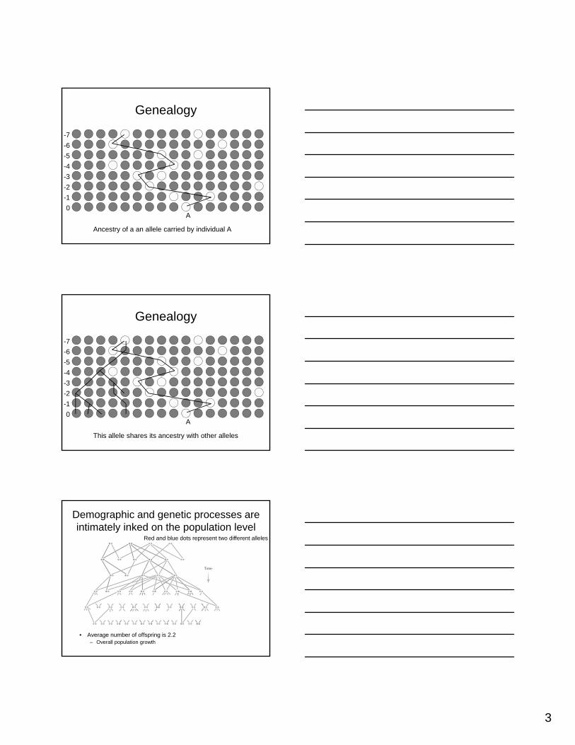
Genealogy

0

-1

-2

-3

-4

-5

-6

-7

Ancestry of a an allele carried by individual A

A

Genealogy

0

-1

-2

-3

-4

-5

-6

-7

This allele shares its ancestry with other alleles

A

Demographic and genetic processes are intimately inked on the population level

• Average number of offspring is 2.2– Overall population growth

Red and blue dots represent two different alleles

4

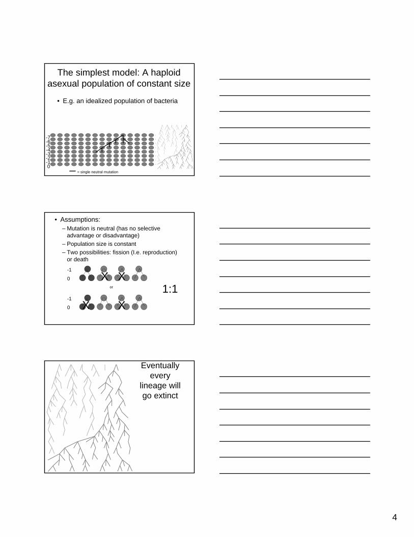
The simplest model: A haploid asexual population of constant size

• E.g. an idealized population of bacteria

0-1-2-3-4-5-6-7

= single neutral mutation

• Assumptions:– Mutation is neutral (has no selective

advantage or disadvantage)

– Population size is constant

– Two possibilities: fission (I.e. reproduction) or death

-1

0 X X

-1

0 X X

or 1:1

Eventually every

lineage will go extinct

5

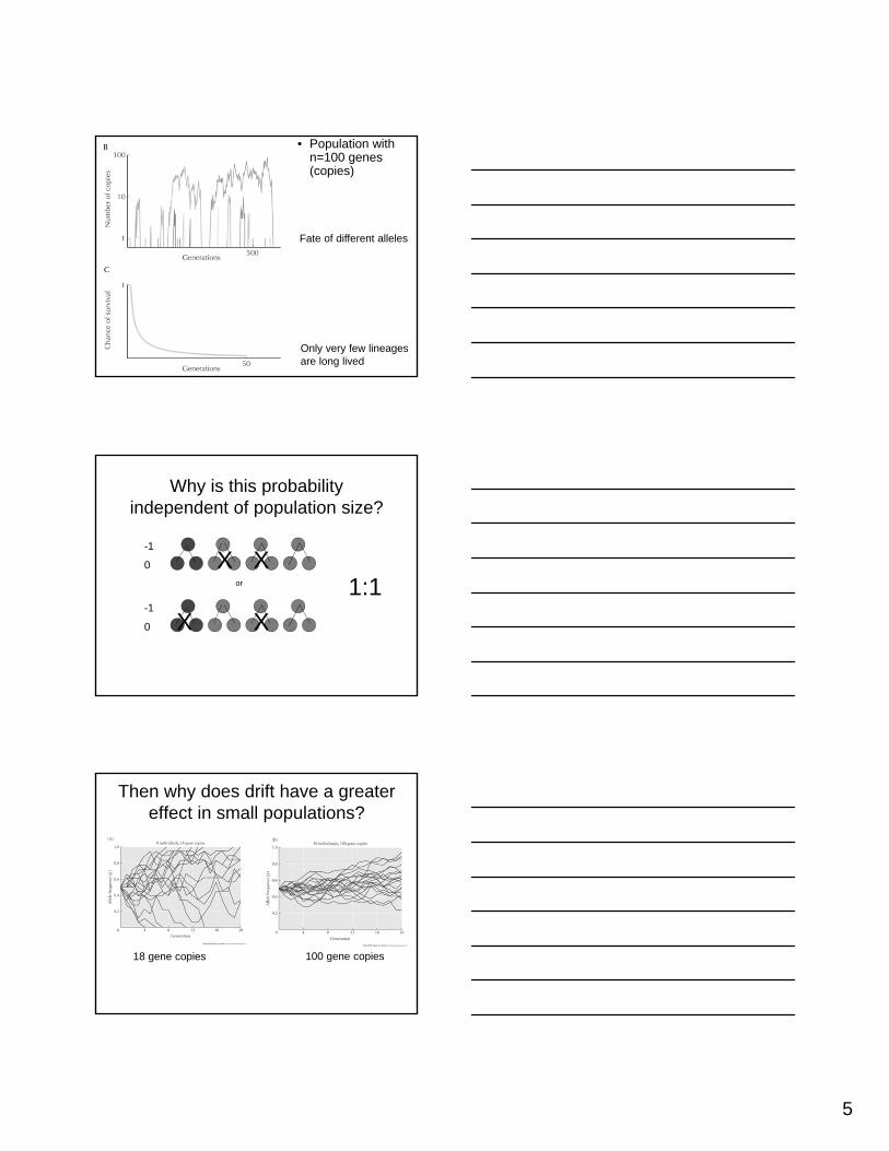
• Population with n=100 genes (copies)

Fate of different alleles

Only very few lineages are long lived

Why is this probability independent of population size?

-1

0 X X

-1

0 X X

or 1:1

Then why does drift have a greater effect in small populations?

18 gene copies 100 gene copies

6

Example: cape buffalo in game reserves of different size

• Microsatellite study by Heller et al. 2010

Example: cape buffalo in game reserves of different size

• Reserves ranged in size from 100 to 28,000 km2

Allelic richness = mean number of alleles across multiple microsatellite loci

In diploid organisms meiosis adds randomness

7

The Wright-Fisher Model

• Assumption: Population size is constant• Assumption: Each individual produces a large

number of gametes• Assumption: Gametes are produced in proportion to

parental allele frequencies• Assumption: Mating of alleles is random• Assumption: Generation are discrete

P Q Q Q

Frequency P = p = #P/2N =0.25 Frequency Q = q = #Q/2N = 0.75

N=2

The Wright-Fisher Model

• Which of the following outcomes is more likely?

= 0.75 x 0.75 x 0.75 x 0.75=0.32

• 0.32

The Wright-Fisher Model

= 0.75 x 0.75 x 0.75 x 0.25=0.105

= 0.75 x 0.75 x 0.75 x 0.25=0.105

= 0.75 x 0.75 x 0.75 x 0.25=0.105

= 0.75 x 0.75 x 0.75 x 0.25=0.105

=0.422

• 0.422

8

The Wright-Fisher Model

• 0.211

= 0.75 x 0.75 x 0.25 x 0.25=0.035

0.035 x 6 = 0.211

The Wright-Fisher Model

= 0.75 x 0.25 x 0.25 x 0.25=0.012

0.012 x 4 = 0.047

• 0.047

The Wright-Fisher Model

• 0.004

= 0.25 x 0.25 x 0.25 x 0.25=0.004

9

The outcome of the Wright-Fisher model is described by

the binomial distribution

• See table 28.1 (online on textbook site)

2N = n

Mean: 2Np

Variance: 2Npq

i = outcome with probability p (e.g. drawing a P allele for the next generation)

The Wright-Fisher model

• The probability for each of the 5 outcomes follows the binomial distribution

Mean=2Np=2*2*0.25=1

1/4=0.25

Mean allele frequency is expected to stay the same

The Wright-Fisher model

• The probability for each of the 5 outcomes follows the binomial distribution

Variance=2Npq=2*2*0.25*0.75=0.75

Variance for allele frequency:(p*q)/2N=(0.25*0.75)/(2*2)=0.047

10

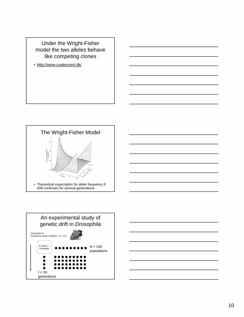
Under the Wright-Fisher model the two alleles behave

like competing clones

• http://www.coalescent.dk/

The Wright-Fisher Model

• Theoretical expectation for allele frequency if drift continues for several generations

An experimental study of genetic drift in Drosophila

8 males x8 females

Generation 0:Frequency brown mutation = p = 0.5

N = 100 populations

t = 19 generations

11

Observed variance of allele frequency in Drosophila experiment does not fit the

expected variance

• But it fits for a smaller than the census population size, the effective population size

In previous generation

Population size 16

Population size 11.5

12

Effective Population size

The size of the ideal Fisher-Wright population that would give the same rate of random drift as the actual population

(I.e. if the census population size and the effective population size do not match the population deviates from the Wright-Fisher model)

Population Size (N) vs. Effective Population Size (Ne)

Ne is what determines the strength of genetic drift

Factors that cause Ne to be less than N

• overlap of generations• variation among indivs in reproductive success

http://www.carnegiemnh.org

http://www.livingwilderness.com

http://wdfw.wa.gov

13

Population Size (N) vs. Effective Population Size (Ne)

Factors that cause Ne to be less than N

• overlap of generations• variation among indivs in reproductive success• unequal sex ratio

http://www.cf.adfg.state.ak.us

Population Size (N) vs. Effective Population Size (Ne)

Factors that cause Ne to be less than N

• overlap of generations• variation among indivs in reproductive success• unequal sex ratio • fluctuations in population size

14

Average N: 725Ne: 404

Population bottlenecks reduce variation and enhance genetic drift

http://www.fws.gov

http://www.nacwg.org

(approx. 1000 indivs in 1850s)

15

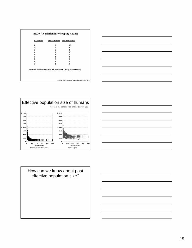
mtDNA variation in Whooping Cranes

Haplotype Pre-bottleneck Post-bottleneck

1 0 122 0 23 5 34 0 1*5 1 06 1 07 2 08 1 09 1 0

*Present immediately after the bottleneck (1951), but not today.

Glenn et al. (1999) Conservation Biology 13: 1097-1107.

Effective population size of humans

Yoruba, NigeriaNorthern and Western Europe

Tenesa et al., Genome Res. 2007. 17: 520-526

How can we know about past effective population size?

16

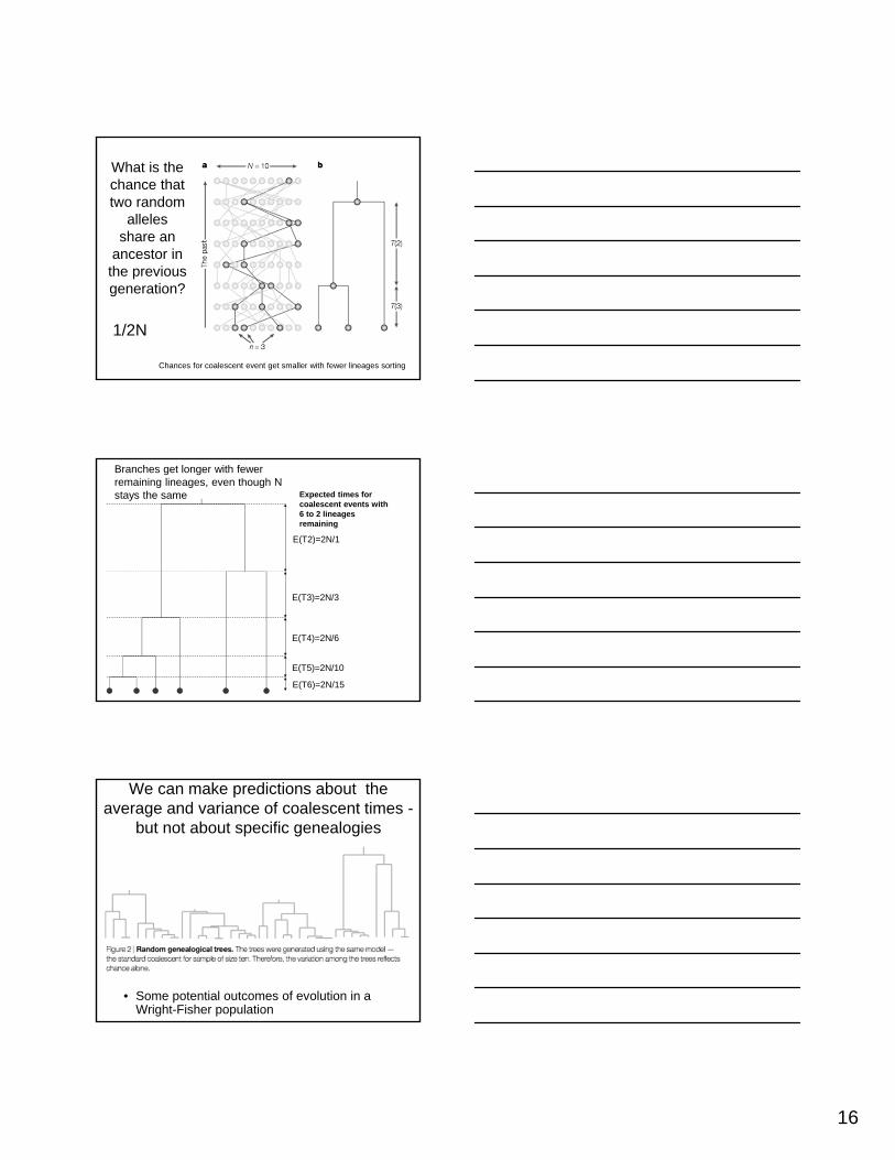
What is the chance that two random

alleles share an

ancestor in the previous generation?

1/2N

Chances for coalescent event get smaller with fewer lineages sorting

E(T2)=2N/1

E(T3)=2N/3

E(T4)=2N/6

E(T5)=2N/10

E(T6)=2N/15

Branches get longer with fewer remaining lineages, even though N stays the same Expected times for

coalescent events with 6 to 2 lineages remaining

We can make predictions about the average and variance of coalescent times -

but not about specific genealogies

• Some potential outcomes of evolution in a Wright-Fisher population

17

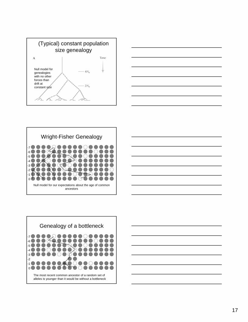
(Typical) constant population size genealogy

Null model for genealogies with no other forces than drift at constant size

Wright-Fisher Genealogy

0

-1

-2

-3

-4

-5

-6

-7

Null model for our expectations about the age of common ancestors

Genealogy of a bottleneck

0

-1

-2

-3

-4

-5

-6

-7

The most recent common ancestor of a random set of alleles is younger than it would be without a bottleneck

18

Bottleneck genealogy

Alleles trace back to a few ancestors in the recent past

bottleneck

The distribution of mutations in alleles can be used to estimate past population size

Many old mutations are shared, but young mutations occur only in certain alleles