Embed Size (px)
Citation preview

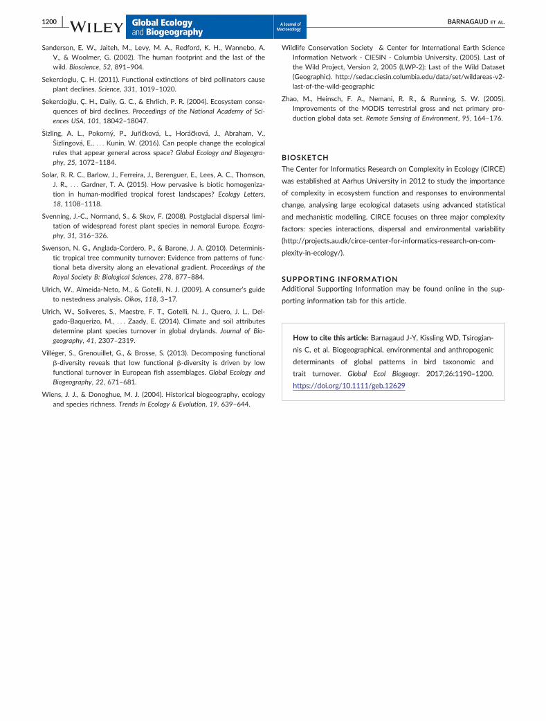
R E S E A R CH PA P E R
Biogeographical, environmental and anthropogenicdeterminants of global patterns in bird taxonomic andtrait turnover
Jean-Yves Barnagaud1,2 | W. Daniel Kissling3 | Constantinos Tsirogiannis4 |
Vissarion Fisikopoulos5 | S�ebastien Vill�eger6 | Cagan H. Sekercioglu7,8 |
Jens-Christian Svenning2
1Biog�eographie et Ecologie des Vert�ebr�es –
UMR 5175 CEFE – CNRS - Universit�e de
Montpellier - EPHE - SupAgro - IND - INRA -
PSL Research University, Montpellier, France
2Section for Ecoinformatics & Biodiversity,
Department of Bioscience, Aarhus
University, Aarhus, Denmark
3Institute for Biodiversity and Ecosystem
Dynamics (IBED), University of Amsterdam,
Amsterdam, The Netherlands
4Center for Massive Data Algorithmics
(MADALGO), Department of Computer
Science, Aarhus University, Aarhus,
Denmark
5D�epartement de Math�ematique, Boulevard
du Triomphe, Universit�e libre de Bruxelles,
Brussels, Belgium
6Laboratoire Biodiversit�e Marine et ses
Usages (MARBEC), UMR 9190 CNRS-IRD-
UM-IFREMER, Universit�e de Montpellier,
Montpellier Cedex 5, , France
7Department of Biology, University of Utah,
Salt Lake City, Utah
8College of Sciences, Koç University,
Rumelifeneri, Istanbul, Sariyer, Turkey
Correspondence
Jean-Yves Barnagaud, Biog�eographie
et Ecologie des Vert�ebr�es – CNRS, PSL
Research University, EPHE, UM, SupAgro,
IND, INRA, UMR 5175 CEFE, 1919 route
de Mende, F34293 Montpellier 5, France.
Email: [email protected]
Funding information
Aarhus University Research Foundation;
VILLUM FONDEN
Editor: Ana Santos
Abstract
Aim: To assess contemporary and historical determinants of taxonomic and ecological trait turn-
over in birds worldwide. We tested whether taxonomic and trait turnover (1) are structured by
regional bioclimatic conditions, (2) increase in relationship with topographic heterogeneity and
environmental turnover and change according to current and historical environmental conditions,
and (3) decrease with human impact.
Major Taxa: Birds.
Location: Global.
Methods: We used computationally efficient algorithms to map the taxonomic and trait turnover
of 8,040 terrestrial bird assemblages worldwide, based on a grid with 110 km3 110 km resolution
overlaid on the extent-of-occurrence maps of 7,964 bird species, and nine ecological traits reflect-
ing six key aspects of bird ecology (diet, habitat use, thermal preference, migration, dispersal and
body size). We used quantile regression and model selection to quantify the influence of biomes,
environment (temperature, precipitation, altitudinal range, net primary productivity, Quaternary
temperature and precipitation change) and human impact (human influence index) on bird
turnover.
Results: Bird taxonomic and trait turnover were highest in the north African deserts and boreal
biomes. In the tropics, taxonomic turnover tended to be higher, but trait turnover was lower than
in other biomes. Taxonomic and trait turnover exhibited markedly different or even opposing rela-
tionships with climatic and topographic gradients, but at their upper quantiles both types of
turnover decreased with increasing human influence.
Main conclusions: The influence of regional, environmental and anthropogenic factors differ
between bird taxonomic and trait turnover, consistent with an imprint of niche conservatism, envi-
ronmental filtering and topographic barriers on bird regional assemblages. Human influence on
these patterns is pervasive and demonstrates global biotic homogenization at a macroecological
scale.
K E YWORD S
Anthropocene, beta diversity, biogeographical legacies, biotic homogenization, functional diversity,
life-history traits, regional assemblages
1190 | VC 2017 JohnWiley & Sons Ltd wileyonlinelibrary.com/journal/geb Global Ecol Biogeogr. 2017;26:1190–1200.
Received: 12 October 2016 | Revised: 5 July 2017 | Accepted: 19 July 2017
DOI: 10.1111/geb.12629

1 | INTRODUCTION
Global biodiversity gradients are shaped from regional to local scales
by the concurrent effects of biogeographical and orographic barriers,
climate and habitat (Caley & Schluter, 1997; Ficetola, Mazel, & Thuiller,
2017; Ricklefs, 2004). However, the accelerating pace of human-driven
global change over the last centuries has deeply modified environmen-
tal filters and species interactions, has created or removed barriers or
broken down old biogeographical boundaries that could affect these
patterns (Capinha, Essl, Seebens, Moser, & Pereira, 2015; Ellis, 2015;
Ficetola et al., 2017). Whether anthropogenic imprint on global biodi-
versity gradients has become comparable to that of ecological and evo-
lutionary processes has therefore become a central question of
macroecology (Ellis, 2015).
Beta diversity, or the compositional difference between two or
more species assemblages, is the most direct and informative measure
of changes in species composition along biodiversity gradients (Koleff,
Gaston, & Lennon, 2003). Depending on the spatial scale, variations in
beta diversity convey signals of habitat composition and biotic interac-
tions, species’ rarity and commonness, metacommunity dynamics or
legacies of speciation/extinction dynamics (Kraft et al., 2011). Beta
diversity can be defined as the additive outcome of two simultaneous
processes: changes in species richness (nestedness-resultant compo-
nent) and changes in species composition (turnover component) (Base-
lga, 2010; Legendre, 2014; Leprieur et al., 2011). These two
components are independent, as an assemblage may be a strict subset
of another (full nestedness) or exhibit the same richness with com-
pletely different species composition (full turnover). They can thus be
analysed separately in the prospect of separating processes that trigger
species richness and compositional variations between assemblages.
While nestedness informs on how species are sorted along environ-
mental or historical gradients from a regional species pool (Svenning,
Normand, & Skov, 2008; Ulrich, Almeida-Neto, & Gotelli, 2009), turn-
over is especially helpful at broad spatial scales to understand how mul-
tiple regional species pools are separated by biogeographical barriers,
environmental gradients and human impact (Antonelli, Nylander, Pers-
son, & Sanmartín, 2009; Caley & Schluter, 1997; Gaston et al., 2007).
Taxonomic turnover is an incomplete measurement of the multi-
faceted structure of biodiversity because it does not reflect variations
in the ecological and evolutionary characteristics of species assemb-
lages (Pavoine & Bonsall, 2011). Trait turnover, or the turnover in spe-
cies’ ecological characteristics or life-history traits, is more appropriate
to investigate non-neutral gradients in assemblage composition, as it
accounts for the ecological non-equivalence of coexisting species (De
Bello et al., 2009). High taxonomic and trait turnovers are expected to
be associated with changes in both resource availability and composi-
tion, such as along altitudinal gradients or other sources of steep envi-
ronmental variation (Swenson, Anglada-Cordero, & Barone, 2010).
However, high taxonomic turnover can be associated with low trait
turnover under the effects of niche-based filtering or as a legacy of his-
torical processes, such as postglacial recolonization events (Vill�eger,
Grenouillet, & Brosse, 2013). Moreover, patterns of trait turnover can
depend on trait selection and resolution. A comparative analysis of
turnover measures computed with different traits that reflect species’
responses to environmental conditions, resource use, dispersal abilities
and biotic interactions is therefore essential to gain a deeper under-
standing of trait turnover (Ackerly & Cornwell, 2007; Lavorel &
Garnier, 2002).
Species assemblages are shaped by broad-scale environmental gra-
dients and by historical legacies related to diversification (speciation
and extinction) and colonization (Ricklefs, 2004; Svenning et al., 2008).
For instance, long-term climatic stability might promote high species
richness and pronounced levels of endemism, especially in the tropics
(Buckley & Jetz, 2007; Kissling, Baker, et al., 2012; Svenning et al.,
2008). Taxonomic turnover can thus be expected to be higher in tropi-
cal than temperate and boreal biomes. In addition, patterns of taxo-
nomic and trait turnover should bear the imprint of glacial refugia and
post-glacial recolonization dynamics as well as of physical barriers
(Antonelli et al., 2009; Baselga, 2010; Buckley & Jetz, 2007). Both
types of turnover are therefore expected to increase along mountain
chains, but also in extremely poor environments, such as deserts,
where low resource availability selects for rarity and small range sizes
(Gaston et al., 2007; Ulrich et al., 2014). Furthermore, niche replace-
ment associated with environmental heterogeneity should translate
into a positive relationship between the steepness of environmental
gradients (i.e., environmental turnover) and taxonomic or trait turnover,
as observed in amphibians and birds (Buckley & Jetz, 2007; Gaston
et al., 2007).
Well-established global diversity patterns, such as Bergmann’s rule
(Blanchet et al., 2010), the diversity–productivity relationship (Pautasso
et al., 2011) or evidence from the fossil record, show a strong human
imprint on biodiversity of our planet (Ellis, 2015; Faurby & Svenning,
2015; �Sizling et al., 2016). Anthropogenic land use decreases net pri-
mary productivity and modifies habitat gradients, favouring common
and widespread species with traits associated with ecological general-
ism (Eskildsen et al., 2015; Haberl et al., 2007). This triggers biotic
homogenization that should, at global and regional scales, result in a
decrease in both taxonomic and trait turnover along gradients of
human impact (Baiser & Lockwood, 2011). However, few studies have
quantitatively compared the influence of biogeographical, environmen-
tal and anthropogenic factors on regional species assemblages (Capinha
et al., 2015).
Here, we quantified global bird taxonomic and trait turnover
among adjacent species assemblages using a moving window approach
(‘neighbourhood turnover’). In doing so, we focused on taxonomic or
trait differences among assemblages that are directly neighbouring
each other, with the aim being to produce a continuous map of compo-
sitional change (as did, e.g., McKnight et al., 2007). We studied the vari-
ation in turnover among biomes and along gradients of environmental
conditions, environmental turnover and anthropogenic influence. We
grounded our study on a global dataset of > 8,000 regional bird
assemblages at 110 km 3 110 km grid cell resolution and on trait data
reflecting habitat use, diet and mobility for > 7,900 species. At this
spatial extent and resolution, we expected bioclimatic and historical
BARNAGAUD ET AL. | 1191

processes to be of key importance for structuring regional bird assemb-
lages (Ricklefs, 2004). We therefore hypothesized that taxonomic and
trait turnover in bird assemblages are structured by biomes, environ-
mental gradients and topography. We tested the following three com-
plementary predictions.
1. The ‘biome hypothesis’: Legacies of biogeographical processes
have triggered biome-level differences in turnover, with high taxo-
nomic and trait turnover in deserts and high taxonomic but low
trait turnover in tropical biomes.
2. The ‘environmental hypothesis’: Taxonomic and trait turnover
increase near topographic barriers and in association with high
environmental turnover. Taxonomic turnover increases and trait
turnover decreases with increasing primary productivity.
3. The ‘biotic homogenization hypothesis’: Taxonomic and trait turn-
over decrease with increasing human impact.
2 | METHODS
2.1 | Data collection
2.1.1 | Bird assemblages
We retrieved global extent-of-occurrence maps for 9,886 bird species
(Birdlife International & Nature Serve, 2012). These data have been
compiled from multiple sources, including specimens, distribution
atlases, survey reports, published literature and expert opinion, and
currently represent the most comprehensive assessment of global bird
species occurrences. We overlaid these maps onto a grid in cylindric
equal area projection with 110 km 3 110 km resolution, corresponding
to 40,680 grid cells (10,599 terrestrial cells), which we used to define
bird assemblages (Kissling, Sekercioglu, & Jetz, 2012). We excluded
Antarctica, cells covering > 50% of water, and cells for which at least
one of the eight neighbours did not have any bird record. We concen-
trated on terrestrial bird assemblages and therefore excluded all pelagic
birds and species related to wetlands that never occur in other terres-
trial habitats. Out of 8,255 terrestrial species, we excluded a further
291 species because of missing trait data (see section 2.1.2), consider-
ing that this additional filter would induce less uncertainty than gap fill-
ing in the trait matrix. This selection resulted in a final matrix of 8,040
cells 3 7,964 species, with an average species richness of 177.86
129.6 (mean6 SD).
2.1.2 | Ecological traits
We recorded the following nine traits that reflect major axes of bird
ecological niches: dietary preference (scores of use summing up to 10
among eight diet categories: invertebrates, fruits, nectar, seeds, vegeta-
tion, fishes, vertebrates and scavenging); Levin’s index of dietary spe-
cialization (Belmaker, Sekercioglu, & Jetz, 2011); habitat use (binary)
among 11 habitat classes arranged along a gradient from forested to
open habitats, derived from the International Union for Conservation
of Nature (IUCN) habitat classification version 3 (Supporting Informa-
tion Appendix S1); preferential vegetation layers (among eight levels
ranging from ground to canopy species); propensity to latitudinal or
altitudinal migrations (three levels: migratory, sedentary or partial
migrant); propensity to irregular dispersal events (three levels: dis-
perser, partial disperser or non-disperser); body mass (in grams); and
thermal preference (average temperature over a species’ range; Barna-
gaud et al., 2014). We acquired these traits from a comprehensive liter-
ature survey covering 8,255 terrestrial bird species (Şekercio�glu, Daily,
& Ehrlich, 2004), corrected and updated with the most recently pub-
lished literature on bird traits (Belmaker et al., 2011; Del Hoyo, Elliott,
& Sargatal, 2013). Most of the data retrieved are averages over multi-
ple individuals with no information on intraspecific variability, which is
beyond the scope and resolution of this study. Among the 291 species
excluded because of missing trait values, 65 species lacked dietary
scores, and five, 18 and two species lacked data for latitudinal migra-
tion, altitudinal migration and irregular movements, respectively. The
remaining 201 missing species were lacking body mass information.
Furthermore, we chose not to include traits related to sociality and
reproductive productivity because of the lack of data for too many spe-
cies. We therefore built our analyses on a complete trait matrix without
relying on gap filling.
2.1.3 | Biogeographical regions
We assigned every grid cell to one of 13 biomes as defined by combi-
nations of coherent climatic and habitat features (World Wide Fund for
Nature, https://www.worldwildlife.org/biomes, updated from Olson
et al., 2001).
2.1.4 | Environmental gradients
We compiled data on current climate (mean annual temperature and
precipitations 1950–2000, from Worldclim, http://www.worldclim.org/),
topography (altitudinal range, Global Land Cover Characterization Data
Base, https://lta.cr.usgs.gov/GLCC), net primary productivity (NPP, from
Moderate-Resolution Imaging Spectroradiometer (MODIS), Zhao,
Heinsch, Nemani, & Running, 2005) and Quaternary climate change
[represented as anomalies, i.e., absolute differences of temperature and
precipitations, between the Last Glacial Maximum (LGM) and the pres-
ent; Ara�ujo et al., 2008; Kissling, Baker, et al., 2012]. The two Quater-
nary climate change variables were calculated across two palaeoclimatic
simulations, the Community Climate System Model version 3 and the
Model for Interdisciplinary Research on Climate version 3.2 (PMIP2;
http://pmip2.lsce.ipsl.fr/; Braconnot et al., 2007). We averaged each
environmental variable across all eight surrounding cells of a focal cell
and the focal cell itself, so that the resolution of environmental assess-
ment matched that of bird turnover.
2.1.5 | Human impact
To estimate human impact, we used the human influence index (HII),
which measures the total amount of anthropogenic footprint accumu-
lated in 1 km2 pixels [Wildlife Conservation Society (WCS), 2005;
updated from Sanderson et al., 2002]. Its computation is extensively
justified elsewhere (Sanderson et al., 2002). In brief, influence scores
from zero (lowest) to 10 (highest) were assessed for eight items consid-
ered to impact wildlife and their habitats directly, based on expert
1192 | BARNAGAUD ET AL.

advice and published literature (11 human population density classes,
proximity to railways, roads, navigable rivers and coastlines, four night-
time light values, inside or outside urban polygons and four land cover
categories). The HII was subsequently computed by summing up these
scores at a 1 km2 grain size. We averaged these HII values to yield a
synthetic measure of the amount of anthropogenic footprint for each
of our 100 km3 100 km grid cells.
2.2 | Turnover computations
2.2.1 | Taxonomic turnover
We computed neighbourhood taxonomic turnover from a decomposi-
tion of neighbourhood beta diversity measured by Jaccard’s dissimilar-
ity index (Baselga, 2012), as follows:
b1ca1b1c
523minimum b; cð Þ
a123minimum b; cð Þ1jb2cja1b1c
3a
a123minimum b; cð Þ (1)
where a is the number of species shared by two adjacent assemblages
which have b and c unique species, respectively, such that a1 b1 c
equals the total species richness among the two communities. In Equa-
tion 1, the first component reflects taxonomic turnover (changes in
species composition irrespective of species richness, ranging from zero,
where one assemblage is a subset of the other, to one, where there are
no shared species) and the second is a nestedness-resultant measure
that accounts for the species richness gradient across the two cells
(beyond the scope of this study). Several alternative frameworks allow
a similar decomposition of Jaccard’s or Sorensen’s dissimilarity indices
and are essentially equivalent in the way they compute turnover
(Legendre, 2014). However, the independence of turnover from spe-
cies richness variations is only ensured by the framework of Baselga
(2012), which we used in this study (Baselga & Leprieur, 2015). We
obtained a unique measure of turnover for each bird assemblage by
averaging pairwise turnovers across each given assemblage and its
eight nearest neighbours. We did not investigate the variation in turn-
over for higher-order neighbourhoods. Although considering a range of
neighbourhood distances smooths the effects of range limits and grain
size (McKnight et al., 2007), meaningful predictions for the relation-
ships between turnover in non-adjacent assemblages and environmen-
tal gradients would be hard to formulate, especially because of the
confounding effects of historical legacies. Also note that computations
of beta diversity indices at multiple neighbourhood orders could
become intractable at the scale of our study.
2.2.2 | Trait turnover
We computed trait dissimilarity between all pairs of species using an
extended version of Gower’s distance that allows dealing with mixed
trait types with adequate weighing to account for structural non-
independencies that typically arise with dietary scores or binary varia-
bles (Pavoine, Vallet, Dufour, Gachet, & Daniel, 2009). We then sum-
marized this dissimilarity matrix with a principal coordinates analysis
(PCoA), from which we retained the three first axes to build a multidi-
mensional trait space that faithfully represents trait-based distance
between species (Supporting Information Appendix S2 displays
correlations of traits with PCoA axes and the amount of variance
explained by each axis).
We computed the turnover component of trait neighbourhood
beta diversity (hereafter ‘neighbourhood trait turnover’ or ‘trait turn-
over’ in our context) as an adaptation of Equation 1 based on the pro-
portion of the trait space (convex hull) shared and not shared by each
bird assemblage and its eight nearest neighbours (Vill�eger et al., 2013),
using species’ scores on the three first axes of the PCoA. This compu-
tation is challenging because calculating the volume of intersection
between convex hulls is disproportionally more difficult than simply
calculating the volume of a single convex hull. Hence, we had to use
elaborate algorithmic methods together with powerful computational
servers. We tested three different convex hull implementations
through Polymake (https://polymake.org) and ended up using the most
efficient for our dataset (Irs: http://cgm.cs.mcgill.ca/~avis/C/lrs.html).
To refine the interpretation of trait turnover patterns, we com-
puted turnover based on five alternative three-dimensional PCoA ordi-
nations built with five distinct subsets of traits: dietary scores (‘diet
turnover’), habitat use (‘habitat turnover’), propensity to migration or
irregular dispersal events (‘mobility turnover’), body mass (‘body mass
turnover’) and thermal preference (‘thermal turnover’). Note that these
additional turnovers were so highly skewed towards zero (see Results)
that we did not subject them to any statistical analysis.
2.2.3 | Environmental turnover
We summarized the six environmental variables into a principal coordi-
nate analysis (PCA), from which we extracted the three first axes, rep-
resenting 81% of total inertia (see Supporting Information Appendix S3
for variable loadings and maps of the raw variables and the principal
components). The first axis (PC1) was dominated by a combination of
temperature, precipitations and primary productivity and opposed trop-
ical to temperate and boreal climates. The second axis (PC2) was a
temperature axis contrasting cells with warm–wet past climates (nega-
tive values) and warm–wet current climates (positive values). The third
axis (PC3) was mostly dominated by topographic heterogeneity (high-
est in negative values). In addition to environmental conditions, we also
quantified environmental turnover by calculating the mean Euclidean
distance of the coordinates of each grid cell with its eight nearest
neighbours on each PC axis (similar to Buckley & Jetz, 2007).
2.3 | Statistical analyses
Scatter plots of taxonomic and trait turnover values against environ-
mental covariates revealed highly skewed distributions, high heterosce-
dasticity and triangular relationships. To overcome these issues, we
used quantile regressions with either taxonomic or trait turnover as the
response variable, using the .10, .25, .50, .75 and .90 quantiles.
We compared four models aimed at a formal comparison of our
biome, environmental and biotic homogenization hypotheses: (a) inter-
cept only (control); (b) biomes only (biome hypothesis); (c) environmental
conditions plus human impact plus biomes (environmental and biotic
homogenization hypotheses); and (d) environmental turnover plus
human impact plus biomes (environmental and biotic homogenization
BARNAGAUD ET AL. | 1193

hypotheses). We made all regression coefficients comparable within
each model by scaling all continuous variables to mean50 and SD51.
The comparison between model (c) and model (d) allowed us to assess
which of environmental turnover, average environmental conditions or
human impact most strongly influenced bird turnover. To control for the
inherent relationship between species and traits, we added taxonomic
turnover as a covariate in models (b), (c) and (d) for trait turnover. We
therefore tested an additional control model (e) for trait turnover, with
taxonomic turnover as a single covariate.
We selected the most parsimonous model on the basis of the
Akaike information criterion (AIC) separately for each quantile. We also
computed an approximate measure of goodness of fit for each quantile
as the ratio of the objective function at the solution (i.e., optimization)
of a given model and the control model (Koenker & Machado, 1999).
We performed all analyses with R 3.3.2 (R Core Team, 2016) and the
package quantreg (Koenker, 2016).
3 | RESULTS
3.1 | Geographical structure of bird turnover
Taxonomic turnover was on average 0.1160.06 (mean 6 SD), ranging
from zero (n512, in North Africa, Arabia and arctic Canada) to 0.51 (n51,
in North Africa), indicating relatively low rates of species replacement
among neighbouring assemblages. The highest taxonomic turnover
occurred in the Andes, eastern North Africa and the Middle East, whereas
Siberia, Europe, North America and Amazonia exhibited comparatively
lower values (Figure 1). Trait turnover was expectedly lower (mean-
50.0260.03; minimum50 in 209 cells spread worldwide; maximum5
0.6, in two North African cells), indicating that adjacent assemblages tend
to have similar trait compositions. Spatial variations in trait turnover were
roughly congruent with taxonomic turnover but were lower in sub-Saharan
Africa and along mountain chains (Figure 2a). However, the two types of
turnover were weakly correlated at the global scale (Pearson’s r2 5 .26),
indicating that changes in the taxonomic composition of bird assemblages
do not adequately reflect associated changes in trait composition.
Spatial variation in trait turnover was equally correlated with turn-
over in habitat (Figure 2b; r25 .45) and dietary (Figure 2c; r25 .44)
preferences. Turnover in migration, dispersal and body mass were all
close to zero except in western and eastern North Africa and the Ara-
bian Peninsula (Figure 2d,e) and therefore contributed little to the
global pattern. Turnover in thermal preferences (Figure 2f) was mostly
structured by mountains and climatic transition regions, such as that
between the Amazonian forest and drier regions of South America
(compare with maps in Supporting Information Appendix S3).
3.2 | Model selection
Models for taxonomic and trait turnover (using all traits) had low fits,
especially at the lowest quantiles, where data tend to be more dis-
persed (adjusted R2 between .03 and .17). Nevertheless, biomes, envi-
ronmental variables and human influence explained substantial
variation in turnover (Table 1, left side, all AIC differences between the
best model and an intercept-only model above 1,600 units). For all
quantiles, the biome effect accounted for approximately one-quarter of
the AIC difference between the intercept-only model and the most-
supported model. Therefore, environmental variation among adjacent
assemblages seemed to have a stronger impact on taxonomic turnover
than coarse bioclimatic differences.
The influence of environmental variables and human influence on
trait turnover increased towards higher quantiles from an AIC differ-
ence of 44.62 (.10 quantile) to 1,604.30 (.90 quantile), in comparison to
a model including biome and taxonomic turnover only (Table 1, right
side). Interestingly, bioclimatic control was strongest for assemblages
with high trait turnover (Table 1; increase in the difference between
models with and without environmental variables of 33.60 to 1,023.30
AIC units from the .10 to the .90 quantiles).
3.3 | Biome hypothesis
Consistent with the biome hypothesis, deserts and xeric shrublands
had the lowest taxonomic and trait turnover of all biomes (Figure 3).
However, while tundra had, as expected, the second highest taxonomic
FIGURE 1 Taxonomic turnover of birds for 8,040 terrestrial assemblages within cells of 110 km 3 110 km resolution. For each cell, turnover iscomputed as the average difference in its bird species composition with its eight nearest neighbours, including all terrestrial species
1194 | BARNAGAUD ET AL.

turnover (Figure 3a), it was associated with the lowest trait turnover
(Figure 3b). Bird assemblages in the high Arctic therefore differ because
of species that share most of their ecological traits, consistent with
large-scale environmental filtering. Interestingly, boreal forests, which
are geographically adjacent to arctic tundra, had the inverse pattern:
low taxonomic turnover (Figure 3a) paired with comparatively high trait
turnover (Figure 3b). All four tropical biomes were spread across the
distribution of taxonomic turnover values (Figure 3a), but for functional
turnover they were in the lower half of the ranking (Figure 3b), in line
with our prediction.
3.4 | Environmental hypothesis
Environmental turnover was positively correlated with all quantiles of
taxonomic turnover (Figure 4a), but it was retained by AIC for the .10,
.25 and .50 quantiles only (Table 1). This result supported the predic-
tion that the steepness of environmental gradients imposes a lower
bound to bird turnover. However, this was not as clear for the lower
quantiles of trait turnover, which either decreased (PC1), increased
(PC2) or did not vary (PC3) with increasing environmental turnover
(Figure 4b). Also consistent with our predictions, environmental condi-
tions imposed an upper limit to taxonomic and trait turnover (Table 1
and Figure 4c,d). Both turnover values decreased from the tropics to
boreal areas (PC1), but whereas taxonomic turnover increased towards
warm and wet areas (PC2) and from high to low topographic heteroge-
neity (PC3), trait turnover decreased along these two gradients.
3.5 | Biotic homogenization hypothesis
Human influence increased both turnover values at lower quantiles
but, consistent with our prediction, decreased them at the .75 and .90
quantiles (Figure 4e,f). Hence, while human impact appeared to trigger
heterogeneity among adjacent bird assemblages that are otherwise
rather homogeneous, it imposed a strong biotic homogenization on
areas with higher taxonomic and trait heterogeneity. Interestingly,
human influence on bird turnover was of the same order of magnitude
(1023) as those of other environmental gradients.
4 | DISCUSSION
Our study unifies previous work on taxonomic turnover (Buckley &
Jetz, 2008), trait turnover (Vill�eger et al., 2013) and the role of large-
scale environmental determinants in shaping regional assemblages
(Hortal, Rodríguez, Nieto-Díaz, & Lobo, 2008). Taxonomic and trait
turnover values among adjacent assemblages were correlated with
dominant bioclimatic gradients and their steepness, consistent with a
major role of bioclimatic filters and physical barriers to dispersal in
shaping global patterns of bird assemblage composition (Pigot, Owens,
FIGURE 2 Trait turnover of birds for 8,040 terrestrial assemblages within cells of 110 km 3 110 km resolution. For each cell, trait turnover iscomputed as the average difference in its bird trait composition with its eight nearest neighbours, including all terrestrial species and (a) all traitsor (b–f) one of five trait subsamples. Trait turnover decreases when fewer traits are considered, demonstrating that functional differencesamong adjacent assemblages are attributable to changes in trait combinations rather than to variations in individual trait pools
BARNAGAUD ET AL. | 1195

& Orme, 2010). Accordingly, neighbourhood trait turnover was domi-
nated by species’ habitat, diet and, to a lesser extent, thermal preferen-
ces in most regions. Importantly, human influence imposed an upper
bound on taxonomic and trait turnover values, as expected under biotic
homogenization.
Consistent with the biome hypothesis, trait turnover was high in
deserts but low in tropical biomes. All traits, and notably those related
to resource use (habitat preference and, to a lesser extent, dietary pref-
erence), showed low turnover rates around the Amazon Basin and in
Southeast Asia in spite of high levels of endemism and resource spe-
cialization (Del Hoyo et al., 2013). Hence, tropical bird assemblages are
relatively homogeneous in traits at the regional scale, which could be
explained by the concurring effects of tropical niche conservatism,TABLE1
Akaikeinform
ationcriterion(AIC)-ba
sedselectionofqu
antile
regressions
forbird
taxo
nomic
andtraitturnove
rwithfive
quan
tiles
Mode
lTax
ono
mic
turnove
rTraitturnove
r
Qua
ntile
.1.25
.5.75
.9.1
.25
.5.75
.9
Env
ironm
ental
turnove
r1HII1
region
225,764.24
226,143.26
224,690.24
221,445.89
217,653.13
248,323.28
246,934.15
243,561.16
237,811.49
231,095.17
Env
ironm
ental
cond
itions
1HII1region
225,765.62
226,093.9
224,596.68
221,454.97
217,796.11
248,322.43
246,917.31
243,565.37
237,891.85
231,242.22
Env
ironm
ental
turnove
r1region
225,718.21
226,113.38
224,680.08
221,447.3
217,601.18
248,318.18
246,935.75
243,553.01
237,733.47
230,831.99
Env
ironm
ental
cond
itions
1region
225,709.75
226,052.89
224,591.46
221,455.54
217,728.14
248,316.4
246,918.61
243,559.25
237,821.09
231,005.62
HII1region
225,489.25
225,765.49
224,265.04
221,024.86
217,146.6
248,320.26
246,919.37
243,520.02
237,710.75
230,932.31
Reg
ion
225,418.56
225,710.13
224,232.28
221,023.35
217,101.81
248,312.29
246,920.85
243,511.54
237,618.93
230,661.13
Taxono
mic
turnove
r2
22
22
248278.66
246758.3
243109.84
236989.66
229637.88
Intercep
tonly
223,970.93
224,344.3
223,041.47
219,616.03
214,903.53
247,795.06
245,427.52
240,844.34
233,799.11
224,896.88
Fit(adjustedR2,
lowestAIC
mode
l).11
.11
.1.11
.17
.03
.09
.16
.16
.16
AIC
5Akaikeinform
ationcriterion;
HII5
human
influe
nceinde
x.Note.
Retaine
dmode
lsareindicatedin
bold,an
dthead
justed
R2is
repo
rted
forthelowestAIC
model.Environmen
talco
nditionsan
den
vi-
ronm
entalturnove
rco
rrespo
ndto
thescoresofthe8,040bird
assemblages
onthreeprincipa
lco
mpo
nent
axes
andtheiraveragedifferen
cewiththeireigh
tnea
rest
neigh
bours.
FIGURE 3 Biome-related variations in bird (a) taxonomic and (b)trait turnover. Differences among biomes are shown as contrastsassessed from quantile regressions (quantile shown5 .5), taking the‘boreal forests and taiga’ (BFT) biome as an arbitrary reference(dashed line). DXS5 deserts and xeric shrublands; FGS5 floodedgrasslands and savannas; MFWS5mediterranean forests,woodlands and scrub; MGS5montane grasslands and shrublands;T5 tundra; TBMF5 temperate broadleaf and mixed forests;TCF5 temperate conifer forests; TGSS5 temperate grasslands,savannas and shrublands; TSCF5 tropical and subtropicalconiferous forests; TSDBF5 tropical and subtropical dry broadleafforests; TSGSS5 tropical and subtropical grasslands, savannas andshrublands; TSMBF5 tropical and subtropical moist broadleafforests
1196 | BARNAGAUD ET AL.

predominance of high rates of local radiation, and low dispersal in the
tropics (Barnagaud et al., 2014; Salisbury, Seddon, Cooney, & Tobias,
2012; Wiens & Donoghue, 2004). These processes have been related
to long-term climatic stability and high resource availability in the tropi-
cal zone (Wiens & Donoghue, 2004). In line with this interpretation,
taxonomic turnover increased while trait turnover decreased towards
warm and wet current climatic conditions. Turnover calculated at finer
resolution (for instance, considering different classes of frugivores or
measurements related to bill size and coloration) would probably yield
more positive correlations between taxonomic and trait turnover if
local specialization on resources and biotic interactions underpin geo-
graphical distributions in tropical bird assemblages (Dehling et al.,
2014). At the other extreme of the climatic gradient, arctic tundra was
also characterized by high taxonomic turnover, but the lowest trait
turnover of all biomes. This was especially true for dietary and habitat
preferences, suggesting strong effects of environmental filtering and
post-glacial recolonization events (Vill�eger et al., 2013).
Taxonomic turnover increased with topographic heterogeneity,
whereas trait turnover decreased. The strong zonation of climatic and
resource conditions in mountains triggers increases in beta diversity
attributable to changes in species richness and species segregation
under the joint effects of thermal and habitat preferences (Dobrovolski,
Melo, Cassemiro, & Diniz-Filho, 2012; Melo, Rangel, & Diniz-Filho,
2009; Swenson et al., 2010). Such patterns are hardly visible at the
spatial resolution of our study because a single bird assemblage in a
mountainous area encompasses the whole range of traits from typical
lowland species to alpine specialists. Consequently, studies within bio-
mes using finer trait classifications and a higher spatial resolution of
species assemblages would probably give different results (Belmaker &
Jetz, 2013; McKnight et al., 2007). Although there was no evidence for
temperature-mediated turnover along altitudinal gradients, turnover in
thermal preferences was higher along biome borders, especially at high
latitudes, the southern border of the Amazonian forest and between
the eastern Sahara and savannahs. This supports the hypothesis of a
FIGURE 4 Environmental effects on (a,c,e) bird taxonomic turnover and (b,d,f) trait turnover as estimated from quantile regressions withfive quantiles. Estimates and 95% confidence intervals (CIs) based on a Gaussian approximation are represented for each tested variable:environmental turnover on three principal component axes (turnover PC1, PC2 and PC3); regional environmental conditions reflected bythese axes (PC1, PC2 and PC3) and human impact quantified by the human influence index. Coefficients corresponding to quantiles thatwere not retained by an Akaike information criterion selection procedure are displayed in grey
BARNAGAUD ET AL. | 1197

relationship between habitat and thermal niches mediated by biogeo-
graphical history (Barnagaud et al., 2012).
As one of multiple forms of biotic homogenization, human-
mediated global change reorganizes bird diversity into more taxonomi-
cally and functionally redundant assemblages (Baiser & Lockwood,
2011; Meynard et al., 2011; Solar et al., 2015). Our results were in line
with this and, furthermore, showed that human influence was the
strongest where taxonomic and trait turnover were highest, such as in
assemblages composed of range-restricted or specialist species, which
usually exhibit low resilience to disturbance (Salisbury et al., 2012) and
are more likely to go extinct (Sekercioglu, 2011). This is notably the
case in deserts and the arctic, where HII is comparably low (Sanderson
et al., 2002), suggesting that small levels of anthropogenic disturbance
have a disproportionate impact on species-poor assemblages. At a
global scale, the magnitude of human influence on bird turnover was
comparable to that of environmental and biogeographical gradients, as
observed in other taxa or at finer spatial scales (�Sizling et al., 2016).
Our results therefore support the hypothesis that a few thousand years
of human imprint on the earth have become a major process structur-
ing biodiversity patterns at macroecological scales (Ellis, 2015) .
5 | CONCLUSION
Although patterns of bird taxonomic turnover have been studied at
various spatial scales (Buckley & Jetz, 2007; Gaston et al., 2007), our
study brings major advances. First, we separated turnover from gra-
dients in species and trait diversity, and could therefore more
adequately address hypotheses that were previously tested globally
using beta diversity as a surrogate of turnover (Gaston et al., 2007;
Koleff, Lennon, & Gaston, 2003). Second, we showed that humans set
a bound to diversity gradients, providing macroecological evidence of
biotic homogenization at a global scale. Our results should stimulate
further assessments of how processes operating at multiple time scales,
including anthropogenic ones, shape present-day turnover of biodiver-
sity across our planet.
DATA ACCESSIBIL ITY
Bird extent of occurrence data can be freely retrieved at http://www.
birdlife.org/datazone/info/spcdownload. All environmental variables
can be retrieved freely on the Internet at the URL provided in the main
text. The species-traits matrix is available upon request from the
authors.
ACKNOWLEDGMENTS
This study is a contribution by the Center for Informatics Research
on Complexity in Ecology (CIRCE), funded by the Aarhus University
Research Foundation under the AU Ideas programme. We are grate-
ful to the Universit�e Libre de Bruxelles for allowing access to its
computation cluster. We thank Simon Chamaill�e-Jammes for advice
on quantile regression. We are grateful to dozens of volunteers and
students, especially Monte Neate-Clegg, Joshua Horns, Evan
Buechley, Jason Socci, Sherron Bullens, Debbie Fisher, David Hayes,
Beth Karpas and Kathleen McMullen, for their dedicated help with
the world bird ecology database. J.-C.S. also considers this work a
contribution to his VILLUM Investigator project ‘Biodiversity Dynam-
ics in a Changing World’ funded by VILLUM FONDEN. W.D.K.
acknowledges a University of Amsterdam starting grant, and Ç.H.S.
acknowledges University of Utah and Koç University support. We
thank Ana Santos and two anonymous referees for their construc-
tive comments on an earlier version of this article.
ORCID
Jean-Yves Barnagaud http://orcid.org/0000-0002-8438-7809
REFERENCES
Ackerly, D. D., & Cornwell, W. K. (2007). A trait-based approach to com-
munity assembly: Partitioning of species trait values into within- and
among-community components. Ecology Letters, 10, 135–145.
Antonelli, A., Nylander, J. A. A., Persson, C., & Sanmartín, I. (2009). Trac-
ing the impact of the Andean uplift on Neotropical plant evolution.
Proceedings of the National Academy of Sciences USA, 106,
9749–9754.
Ara�ujo, M. B., Nogu�es-Bravo, D., Diniz-Filho, J. A. F., Haywood, A. M.,
Valdes, P. J., & Rahbek, C. (2008). Quaternary climate changes
explain diversity among reptiles and amphibians. Ecography, 31,
8–15.
Baiser, B., & Lockwood, J. L. (2011). The relationship between functional
and taxonomic homogenization. Global Ecology and Biogeography, 20,
134–144.
Barnagaud, J.-Y., Devictor, V., Jiguet, F., Barbet-Massin, M., Le Viol, I., &
Archaux, F. (2012). Relating habitat and climatic niches in birds. PLoS
One, 7, e32819.
Barnagaud, J.-Y., Kissling, W. D., Sandel, B., Eiserhardt, W. L., Şeker-cio�glu, Ç. H., Enquist, B. J., & Svenning, J. C. (2014). Ecological traits
influence the phylogenetic structure of bird species co-occurrences
worldwide. Ecology Letters, 17, 811–820.
Baselga, A. (2010). Partitioning the turnover and nestedness components
of beta diversity. Global Ecology and Biogeography, 19, 134–143.
Baselga, A. (2012). The relationship between species replacement, dis-
similarity derived from nestedness, and nestedness. Global Ecology
and Biogeography, 21, 1223–1232.
Baselga, A., & Leprieur, F. (2015). Comparing methods to separate
components of beta diversity. Methods in Ecology and Evolution, 6,
1069–1079.
Belmaker, J., & Jetz, W. (2013). Spatial scaling of functional structure
in bird and mammal assemblages. The American Naturalist, 181,
464–478.
Belmaker, J., Sekercioglu, C. H., & Jetz, W. (2011). Global patterns of
specialization and coexistence in bird assemblages. Journal of Biogeog-
raphy, 39, 193–203.
Birdlife International & NatureServe. (2012). Bird species distribution maps
of the world. Version 2.0. BirdLife International, Cambridge, UK and
NatureServe, Arlington, USA.
Blanchet, S., Grenouillet, G., Beauchard, O., Tedesco, P. A., Leprieur, F.,
D€urr, H. H., . . . Brosse, S. (2010). Non-native species disrupt the
worldwide patterns of freshwater fish body size: Implications for
Bergmann’s rule. Ecology Letters, 13, 421–431.
1198 | BARNAGAUD ET AL.

Braconnot, P., Otto-Bliesner, B., Harrison, S., Joussaume, S., Peterchmitt,
J.-Y., Abe-Ouchi, A., . . . Zhao, Y. (2007). Results of PMIP2 coupled
simulations of the Mid-Holocene and Last Glacial Maximum – Part 1:
Experiments and large-scale features. Climate of the Past, 3,
261–277.
Buckley, L. B., & Jetz, W. (2007). Environmental and historical constraints
on global patterns of amphibian richness. Proceedings of the Royal
Society B: Biological Sciences, 274, 1167–1173.
Buckley, L. B., & Jetz, W. (2008). Linking global turnover of species and
environments. Proceedings of the National Academy of Sciences USA,
105, 17836–17841.
Caley, M. J., & Schluter, D. (1997). The relationship between local and
regional diversity. Ecology, 78, 70–80.
Capinha, C., Essl, F., Seebens, H., Moser, D., & Pereira, H. M. (2015). The
dispersal of alien species redefines biogeography in the Anthropo-
cene. Science, 348, 1248–1251.
De Bello, F., Thuiller, W., Lep�s, J., Choler, P., Cl�ement, J.-C., Macek, P.,
. . . Lavorel, S. (2009). Partitioning of functional diversity reveals the
scale and extent of trait convergence and divergence. Journal of Veg-
etation Science, 20, 475–486.
Dehling, D. M., Fritz, S. A., T€opfer, T., Päckert, M., Estler, P., B€ohning-
Gaese, K., & Schleuning, M. (2014). Functional and phylogenetic
diversity and assemblage structure of frugivorous birds along an ele-
vational gradient in the tropical Andes. Ecography, 37, 1047–1055.
Del Hoyo, J., Elliott, A., & Sargatal, J. (2013). Handbook of the birds of the
world. Barcelona, Spain: Lynx Edicions.
Dobrovolski, R., Melo, A. S., Cassemiro, F. A. S., & Diniz-Filho, J. A. F.
(2012). Climatic history and dispersal ability explain the relative
importance of turnover and nestedness components of beta diver-
sity. Global Ecology and Biogeography, 21, 191–197.
Ellis, E. C. (2015). Ecology in an anthropogenic biosphere. Ecological
Monographs, 85, 287–331.
Eskildsen, A., Carvalheiro, L. G., Kissling, W. D., Biesmeijer, J. C.,
Schweiger, O., & Høye, T. T. (2015). Ecological specialization matters:
Long-term trends in butterfly species richness and assemblage com-
position depend on multiple functional traits. Diversity and Distribu-
tions, 21, 792–802.
Faurby, S., & Svenning, J.-C. (2015). Historic and prehistoric human-
driven extinctions have reshaped global mammal diversity patterns.
Diversity and Distributions, 21, 1155–1166.
Ficetola, G. F., Mazel, F., & Thuiller, W. (2017). Global determinants of
zoogeographical boundaries. Nature Ecology & Evolution, 1, 0089.
Gaston, K. J., Davies, R. G., Orme, C. D. L., Olson, V. A., Thomas, G. H., Ding,
T.-S., . . . Blackburn, T. M. (2007). Spatial turnover in the global avifauna.
Proceedings of the Royal Society B: Biological Sciences, 274, 1567–1574.
Haberl, H., Erb, K. H., Krausmann, F., Gaube, V., Bondeau, A., Plutzar, C.,
. . . Fischer-Kowalski, M. (2007). Quantifying and mapping the human
appropriation of net primary production in earth’s terrestrial ecosys-
tems. Proceedings of the National Academy of Sciences USA, 104,
12942–12947.
Hortal, J., Rodríguez, J., Nieto-Díaz, M., & Lobo, J. M. (2008). Regional
and environmental effects on the species richness of mammal
assemblages. Journal of Biogeography, 35, 1202–1214.
Kissling, W. D., Baker, W. J., Balslev, H., Barfod, A. S., Borchsenius, F.,
Dransfield, J., . . . Svenning, J.-C. (2012). Quaternary and pre-
quaternary historical legacies in the global distribution of a major
tropical plant lineage. Global Ecology and Biogeography, 21, 909–921.
Kissling, W. D., Sekercioglu, C. H., & Jetz, W. (2012). Bird dietary guild
richness across latitudes, environments and biogeographic regions.
Global Ecology and Biogeography, 21, 328–340.
Koenker, R. (2016). quantreg: Quantile Regression. R package version
5.29. https://CRAN.R-project.org/package5quantreg
Koenker, R., & Machado, J. A. F. (1999). Goodness of fit and related
inference processes for quantile regression. Journal of the American
Statistical Association, 94, 1296–1310.
Koleff, P., Gaston, K. J., & Lennon, J. J. (2003). Measuring beta diversity
for presence–absence data. Journal of Animal Ecology, 72, 367–382.
Koleff, P., Lennon, J. J., & Gaston, K. J. (2003). Are there latitudinal
gradients in species turnover? Global Ecology and Biogeography, 12,
483–498.
Kraft, N. J. B., Comita, L. S., Chase, J. M., Sanders, N. J., Swenson, N. G.,
Crist, T. O., . . . Myers, J. A. (2011). Disentangling the drivers of b
diversity along latitudinal and elevational gradients. Science, 333,
1755–1758.
Lavorel, S., & Garnier, E. (2002). Predicting changes in community com-
position and ecosystem functioning from plant traits: Revisiting the
Holy Grail. Functional Ecology, 16, 545–556.
Legendre, P. (2014). Interpreting the replacement and richness difference
components of beta diversity. Global Ecology and Biogeography, 23,
1324–1334.
Leprieur, F., Tedesco, P. A., Hugueny, B., Beauchard, O., D€urr, H. H.,
Brosse, S., & Oberdorff, T. (2011). Partitioning global patterns of
freshwater fish beta diversity reveals contrasting signatures of past
climate changes. Ecology Letters, 14, 325–334.
McKnight, M. W., White, P. S., McDonald, R. I., Lamoreux, J. F., Sechrest,
W., Ridgely, R. S., & Stuart, S. N. (2007). Putting beta-diversity on
the map: Broad-scale congruence and coincidence in the extremes.
PLoS Biology, 5, e272.
Melo, A. S., Rangel, T. F. L. V. B., & Diniz-Filho, J. A. F. (2009). Environ-
mental drivers of beta-diversity patterns in New-World birds and
mammals. Ecography, 32, 226–236.
Meynard, C. N., Devictor, V., Mouillot, D., Thuiller, W., Jiguet, F., & Mou-
quet, N. (2011). Beyond taxonomic diversity patterns: How do a, b
and g components of bird functional and phylogenetic diversity
respond to environmental gradients across France? Global Ecology
and Biogeography, 893–903.
Olson, D. M., Dinerstein, E., Wikramanayake, E. D., Burgess, N. D.,
Powell, G. V. N., Underwood, E. C., . . . Kassem, K. R. (2001). Terres-
trial ecoregions of the worlds: A new map of life on Earth. Bioscience,
51, 933–938.
Pautasso, M., B€ohning-Gaese, K., Clergeau, P., Cueto, V. R., Dinetti, M.,
Fern�andez-Juricic, E., . . . Cantarello, E. (2011). Global macroecology
of bird assemblages in urbanized and semi-natural ecosystems. Global
Ecology and Biogeography, 20, 426–436.
Pavoine, S., & Bonsall, M. B. (2011). Measuring biodiversity to explain
community assembly: A unified approach. Biological Reviews, 86,
792–812.
Pavoine, S., Vallet, J., Dufour, A.-B., Gachet, S., & Daniel, H. (2009). On the
challenge of treating various types of variables: Application for improv-
ing the measurement of functional diversity. Oikos, 118, 391–402.
Pigot, A. L., Owens, I. P. F., & Orme, C. D. L. (2010). The environmental
limits to geographic range expansion in birds. Ecology Letters, 13,
705–715.
R Core Team. (2016). R: A language and environment for statistical com-
puting. Vienna, Austria: R Foundation for Statistical Computing.
Ricklefs, R. E. (2004). A comprehensive framework for global patterns in
biodiversity. Ecology Letters, 7, 1–15.
Salisbury, C. L., Seddon, N., Cooney, C. R., & Tobias, J. A. (2012). The lat-
itudinal gradient in dispersal constraints: Ecological specialisation
drives diversification in tropical birds. Ecology Letters, 15, 847–855.
BARNAGAUD ET AL. | 1199
Sanderson, E. W., Jaiteh, M., Levy, M. A., Redford, K. H., Wannebo, A.
V., & Woolmer, G. (2002). The human footprint and the last of the
wild. Bioscience, 52, 891–904.
Sekercioglu, Ç. H. (2011). Functional extinctions of bird pollinators cause
plant declines. Science, 331, 1019–1020.
Şekercio�glu, Ç. H., Daily, G. C., & Ehrlich, P. R. (2004). Ecosystem conse-
quences of bird declines. Proceedings of the National Academy of Sci-
ences USA, 101, 18042–18047.
�Sizling, A. L., Pokorn�y, P., Ju�ričkov�a, L., Hor�ačkov�a, J., Abraham, V.,�Sizlingov�a, E., . . . Kunin, W. (2016). Can people change the ecological
rules that appear general across space? Global Ecology and Biogeogra-
phy, 25, 1072–1184.
Solar, R. R. C., Barlow, J., Ferreira, J., Berenguer, E., Lees, A. C., Thomson,
J. R., . . . Gardner, T. A. (2015). How pervasive is biotic homogeniza-
tion in human-modified tropical forest landscapes? Ecology Letters,
18, 1108–1118.
Svenning, J.-C., Normand, S., & Skov, F. (2008). Postglacial dispersal limi-
tation of widespread forest plant species in nemoral Europe. Ecogra-
phy, 31, 316–326.
Swenson, N. G., Anglada-Cordero, P., & Barone, J. A. (2010). Determinis-
tic tropical tree community turnover: Evidence from patterns of func-
tional beta diversity along an elevational gradient. Proceedings of the
Royal Society B: Biological Sciences, 278, 877–884.
Ulrich, W., Almeida-Neto, M., & Gotelli, N. J. (2009). A consumer’s guide
to nestedness analysis. Oikos, 118, 3–17.
Ulrich, W., Soliveres, S., Maestre, F. T., Gotelli, N. J., Quero, J. L., Del-
gado-Baquerizo, M., . . . Zaady, E. (2014). Climate and soil attributes
determine plant species turnover in global drylands. Journal of Bio-
geography, 41, 2307–2319.
Vill�eger, S., Grenouillet, G., & Brosse, S. (2013). Decomposing functional
b-diversity reveals that low functional b-diversity is driven by low
functional turnover in European fish assemblages. Global Ecology and
Biogeography, 22, 671–681.
Wiens, J. J., & Donoghue, M. J. (2004). Historical biogeography, ecology
and species richness. Trends in Ecology & Evolution, 19, 639–644.
Wildlife Conservation Society & Center for International Earth Science
Information Network - CIESIN - Columbia University. (2005). Last of
the Wild Project, Version 2, 2005 (LWP-2): Last of the Wild Dataset
(Geographic). http://sedac.ciesin.columbia.edu/data/set/wildareas-v2-
last-of-the-wild-geographic
Zhao, M., Heinsch, F. A., Nemani, R. R., & Running, S. W. (2005).
Improvements of the MODIS terrestrial gross and net primary pro-
duction global data set. Remote Sensing of Environment, 95, 164–176.
BIOSKETCH
The Center for Informatics Research on Complexity in Ecology (CIRCE)
was established at Aarhus University in 2012 to study the importance
of complexity in ecosystem function and responses to environmental
change, analysing large ecological datasets using advanced statistical
and mechanistic modelling. CIRCE focuses on three major complexity
factors: species interactions, dispersal and environmental variability
(http://projects.au.dk/circe-center-for-informatics-research-on-com-
plexity-in-ecology/).
SUPPORTING INFORMATIONAdditional Supporting Information may be found online in the sup-
porting information tab for this article.
How to cite this article: Barnagaud J-Y, Kissling WD, Tsirogian-
nis C, et al. Biogeographical, environmental and anthropogenic
determinants of global patterns in bird taxonomic and
trait turnover. Global Ecol Biogeogr. 2017;26:1190–1200.
https://doi.org/10.1111/geb.12629
1200 | BARNAGAUD ET AL.