Biogeochemical Modelling of Ria Formosa (South Coast of Portugal) with EcoDynamo

Model description

Pedro Duarte, António Pereira, Manuela Falcão, Dalila Serpa, Catarina Ribeiro, Rui Bandeira and Bruno Azevedo

University Fernando Pessoa, Centre for Modelling and

Analysis of Environmental Systems

June 2006 DITTY (Development of an information technology tool for the

management of Southern European lagoons under the influence of river-basin runoff) (EESD Project EVK3-CT-2002-00084)

Summary In this work a biogeochemical model of Ria Formosa (South of Portugal) is presented. Ria Formosa is a large (c.a. 100 km2) mesotidal lagunary system with large intertidal areas and several conflicting uses, such as fisheries, aquaculture, tourism and nature conservation. This coastal ecosystem is a natural park where several management plans and administrative responsibilities overlap. The work presented here is part of a coupled hydrodynamic-biogeochemical model that includes pelagic and benthic processes and variables. It is a two-dimensional vertically integrated model, based on a finite differences grid with a 100 m spatial step and a semi-implicit resolution scheme. It is forced by conditions at the sea boundary, river and water treatment plant discharges, wind speed, light intensity and air temperature. The model includes a wet-drying scheme to account for the dynamics of the large intertidal areas. The purposes of this work are to describe the biogeochemical model and how it has been coupled with a hydrodynamic model, discuss its structure and present some calibration exercises.

CONTENTS

1 Introduction ................................................................................................................ 1 1.1 Site description ..................................................................................................... 1 1.2 Objectives ............................................................................................................. 2

2 Methodology............................................................................................................... 2 2.1 Model software description and implementation ................................................. 3 2.2 Biogeochemical model description ...................................................................... 8

2.2.1. Hydrodynamic object ................................................................................. 24 2.2.2. Wind object................................................................................................. 24 2.2.3. Air temperature object ................................................................................ 24 2.2.4. Light intensity and water temperature objects............................................ 24 2.2.5 Dissolved substances object ....................................................................... 24 2.2.6 Suspended matter object................................................................................. 25 2.2.7 Phytoplankton object .................................................................................. 26 2.2.8 Enteromorpha spp. and Ulva spp. objects ................................................. 27 2.2.9 Zostera noltii object.................................................................................... 27 2.2.10 Ruditapes decussatus object ...................................................................... 27

2.3 Model setup ........................................................................................................ 28 2.4 Model testing ...................................................................................................... 31

3 Results and discussion.............................................................................................. 32 4 References ................................................................................................................ 44

1

1 Introduction

This work is part of the DITTY project “Development of an Information Technology

Tool for the Management of European Southern Lagoons under the influence of river-

basin runoff” (http://www.dittyproject.org/). The general objective of DITTY is the

development of information technology tools integrating Databases, Geographical

Information Systems (GIS), Mathematical Models and Decision Support Systems to

help in the management of southern European coastal lagoons and adjacent watersheds,

within the objectives of the Water Framework Directive (UE, 2000).

The DITTY project takes place at five southern European coastal lagoons. The work

presented here concerns the biogeochemical modelling of Ria Formosa – the Portuguese

case study within DITTY (Fig. 1-1).

1.1 Site description

Ria Formosa is a shallow mesotidal lagoon located at the south of Portugal (Algarve

coast) with a wet area of 10 500 ha (Figure 1-1). The lagoon has several channels and a

large intertidal area, which corresponds roughly to 50% of the total area, mostly covered

by sand, muddy sand-flats and salt marshes. The intertidal area is exposed to the

atmosphere for several hours, over each semi-diurnal tidal period, due to its gentle

slopes. Salinity remains close to 36 ppt, except during sporadic and short periods of

winter run-off. Tidal amplitude varies from 1 to 3.5 meters and the mean water depth is

3.5 m.

2

8.05 8.00 7.95 7.90 7.85 7.80 7.75 7.70 7.65 7.60 7.55 7.50

Longitude (ºW)

36.95

37.00

37.05

37.10

37.15

37.20

Latit

u de

(ºN

)

I1I2

Atlantic OceanI3

I4

I5

I6

III 111 ––– SSS... LLLuuuííísss IIInnnlll eeetttIII 222 ––– FFFaaarrrooo---OOOlllhhhãããoooIIInnnlll eeetttIII 333 ––– AAArrrmmmooonnnaaa IIInnnlll eeetttIII 444 ––– FFFuuuzzzeeetttaaa IIInnnlll eeetttIII 555 ––– TTTaaavvviii rrraaa IIInnnllleeetttIII 666 ––– CCCaaaccceeelll aaa IIInnnlll eeettt

FaroOlhão

Tavira

Marim

Cacela

ncão

RFFuzeta

8.05 8.00 7.95 7.90 7.85 7.80 7.75 7.70 7.65 7.60 7.55 7.50

Longitude (ºW)

36.95

37.00

37.05

37.10

37.15

37.20

Latit

u de

(ºN

)

8.05 8.00 7.95 7.90 7.85 7.80 7.75 7.70 7.65 7.60 7.55 7.50

Longitude (ºW)

36.95

37.00

37.05

37.10

37.15

37.20

Latit

u de

(ºN

)

I1I2

Atlantic OceanI3

I4

I5

I6

III 111 –

I1I2

Atlantic OceanI3

I4

I5

I6

III 111 ––– SSS... LLLuuuííísss IIInnnlll eeetttIII 222 ––– FFFaaarrrooo---OOOlllhhhãããoooIIInnnlll eeetttIII 333 ––– AAArrrmmmooonnnaaa IIInnnlll eeetttIII 444 ––– FFFuuuzzzeeetttaaa

–– SSS... LLLuuuííísss IIInnnlll eeetttIII 222 ––– FFFaaarrrooo---OOOlllhhhãããoooIIInnnlll eeetttIII 333 ––– AAArrrmmmooonnnaaa IIInnnlll eeetttIII 444 ––– FFFuuuzzzeeetttaaa IIInnnlll eeetttIII 555 ––– TTTaaavvviii rrraaa IIInnnllleeetttIII 666 ––– CCCaaaccceeelll aaa IIInnnlll eeettt

FaroOlhão

Tavira

Marim

Cacela

ncão

RFFuzeta

Figure 1-1- Geographic location of Ria Formosa and its inlets (I1 – I6).

1.2 Objectives The purposes of this work are to describe a biogeochemical model implemented for Ria

Formosa and how it has been coupled with a hydrodynamic model, discuss its structure

and present some calibration exercises.

2 Methodology The biogeochemical model implemented in this work is a two dimensional vertically

integrated model based on a finite difference staggered grid, as described previously for

the hydrodynamic model (cf. – Duarte et al, 2005), that calculates the velocity field with

the equations of motion and the equation of continuity (Knauss, 1997) and solves the

transport equation for all pelagic variables:

( ) ( ) 2 2

2 2uS vSdS S S

Sources SinksA Ax ydt x y x y

∂ ∂ ∂ ∂+ + = + + −∂ ∂ ∂ ∂

(1)

3

Where,

u and v - current speeds in x (West-East) and y (South-North) directions (m s-1); A –

Coefficient of eddy diffusivity (m2 s-1); S – A conservative (Sources and Sinks are null)

or a non conservative variable in the respective concentration units.

The biogeochemical model provides the values for the Sources and Sinks terms of

equation 1 at each grid cell.

2.1 Model software description and implementation

The model was implemented using EcoDynamo (Pereira & Duarte, 2005). EcoDynamo

uses Object Oriented Programming (OOP) to relate a set of "ecological" objects by

means of a server or shell, which allows these to interact with each other, and displays

the results of their interaction. Both the EcoDynamo shell and the objects have been

programmed in C++ for WindowsTM. There are different objects to simulate

hydrodynamic, thermodynamic and biogeochemical processes and variables. The shell

interface allows the user to choose among different models and to define the respective

setups – time steps, output formats (file, graphic and tables), objects to be used and

variables to be visualised. The objects used in the present model are listed in Table 2-1

and described below. The physical and biogeochemical processes simulated by the

model are presented in Figs. 2-2 and 2-3. Differential equations for water column, pore

water, sediment and benthic variables are shown in Tables 2-2 – 2-5. Part of these

equations (those concerning pelagic state variables), represent the sources-sinks terms of

Equation 1. The corresponding rate equations are presented in Tables 2-6 – 2-9. Model

parameters are listed in Table 2-10.

4

Table 2-1 – EcoDynamo objects implemented for Ria Formosa and respective variable outputs (see text).

Object type Object name Object outputs Wind object Wind speed Air temperature object Air temperature Water temperature object Radiative fluxes and balance

between water and atmosphere and water temperature

Light intensity object Total and photosynthetically active radiation (PAR) at the surface and at any depth

Tide object Tidal height

Objects providing forcing functions

Salt marsh object Nitrate consumption, ammonia and suspended matter release

Hydrodynamic 2D object Sea level, current speed and direction

Sediment biogeochemistry object Pore water dissolved inorganic nitrogen (ammonia, nitrate and nitrite), inorganic phosphorus and oxygen, sediment adsorbed inorganic phophorus, organic phosphorus, nitrogen and carbon

Dissolved substances object Dissolved inorganic nitrogen (ammonia, nitrate and nitrite), inorganic phosphorus and oxygen

Suspended matter object Total particulate matter (TPM), particulate organic matter (POM), carbon (POC), nitrogen (PON),phosphorus (POP) and the water light extinction coefficient

Objects providing state variables

Phytoplankton object Phytoplankton biomass, productivity and cell nutrient quotas

Enteromorpha sp. object Macroalgal biomass, productivity and cell nutrient quotas

Ulva sp. object Macroalgal biomass, productivity and cell nutrient quotas

Zostera noltti object Macrophyte biomass and numbers, cell nutrient quotas and demographic fluxes

Clams (Ruditapes decussatus) object Clam size, biomass, density, filtration, feeding, assimilation and scope for growth

5

Phytoplankton

Enteromorpa sp. Ulva sp. Zostera nolti

Salt marsh

Ruditapesdecussatus

NH4S NO3S

PO4S O2SNorgS PorgS

NH4WNO3W

PO4W

O2W

CorgS

CorgWdet

NorgWdet

PorgWdet

NPhyto CPhyto PPhyto

POM

NEnt CEnt PEnt NUlva CUlva PUlva NZos CZos PZos

Fig. 2-1 - Biogeochemical processes and variables simulated by the model. The name of the variables is the same as in Tables 2-2 – 2-8. The prefix N, C, and P refers to Nitrogen, Carbon and Phosphorus. The subscripts w and s refer to water column or

sediment variables.

Given the large intertidal areas of Ria Formosa (cf. – 1.1 Site description), the model

includes a wet-drying scheme that prevents any grid cell from running completely dry,

avoiding numerical errors. The general approach is to stop using the advection term

when depth is lower than a threshold value (0.1 m in the present case) to avoid

numerical instabilities. Below this threshold and until a minimum limit of 0.05 m, the

model computes all remaining terms. When this limit is reached, computations do not

take place in a given cell until a neighbour cell has a higher water level, allowing then

the pressure term to start “filling” the “dry” cell.

This hydrodynamic model is forced by water level and river discharges at sea and land

boundaries, respectively. The former are calculated by the equations and the harmonic

components for the Faro-Olhão harbour (cf. – Fig.1-1) described in SHOM (1984) and

listed in a previous report (Duarte et al., 2005). Biogeochemical processes are forced by

6

sea-lagoon exchanges, river discharges, air-water heat and mass exchanges and light

intensity.

NH4S

NO3S

PO4S

O2S

NH4WNO3W PO4W O2W

NO3S

NH4S PO4S

O2S

Water

1st Sedimentlayer

2nd Sedimentlayer

Water-air mass diffusion

Water-sediment diffusion

Sediment-sediment diffusion

NorgPorgSCorgS

Deposition/Resuspension

CorgWdet

NorgWdet

PorgWdet

Horizontal advectionand turbulent diffusion

Fig. 2-2 - Physical and biogeochemical processes and variables simulated by the model. The name of the variables is the same as in Tables 2 – 5. The prefix N, C, and P refers to

Nitrogen, Carbon and Phosphorus. The subscripts w and s refer to fluxes in the water column or in sediment layers.

The wet-drying scheme referred above requires a relatively high spatial and temporal

resolution. In the present case, the former is 100 m and the latter 3 s. A lower temporal

resolution leads to numerical errors, in spite of the semi-implicit numerical scheme of

the hydrodynamic model (Duarte et al., 2005). Therefore, the model requires a large

computing time. Several steps were taken to reduce the computational costs: (i) To

subdivide Ria Formosa in two subsystems – the western and the eastern Ria - as

described in a previous report (Duarte et al., 2005); (ii) To run biogeochemistry only for

the part of the model domain covering the precise area of Ria Formosa; (iii) To run only

the hydrodynamic part of the model, save the results and “rewind” them later to provide

7

the hydrodynamic forcing for the biogeochemical simulations (cf. - 2.2.1 Hydrodynamic

object) and (iv) To produce a multi- processing version of EcoDynamo.

In what concerns the first step, Ria Formosa was indeed sub-divided. In the present

work it was considered only the “Western Ria” (Fig. 2-3).

Lagoon Water Quality Stations sampled in 1992.

Lagoon Sediment, Sediment Fluxes andPore Water Stations, sampled in 2001.

RA Station

RC Station

RB Station

Lagoon Sediment, Sediment Fluxes andPore Water Stations, sampled in 2001.

RA Station

RC Station

RB Station

Water Quality Stations sampled in 1992, used inthe model as boundary conditions.

30 km

Land and river boundaries

Wes

tern

sea

boun

dar

y

Eas

tern

sea

bou

ndar

y

Southern sea boundary

Fig. 2-3 – Model domain covering a total area of 546 km2 (whole rectangle) and 98 km2 (only the area of covered by the lagoon), for the hydrodynamic and biogeochemical

simulations, respectively. Spatial resolution is 100 mm. Time step is 3 and 30 seconds for the hydrodynamic and the biogeochemical simulations, respectively (see text).

Regarding the second step, it is possible to run only a part of the model domain, by

defining a sub-domain, allowing a much faster simulation of biogeochemical processes.

In the present case, sub-domain shape matches exactly the shape of the Western Ria

Formosa. However, current velocity data must be available for transport calculations

(equation 1) (cf. - 2.2.1 Hydrodynamic object). Pereira & Duarte (2005) describe how to

run a sub-domain with the EcoDynamo shell. Rodrigues et al. (2005) describe how to

produce a text file of coordinates using ArcGIS that may be handled with EcoDynamo

as a sub-domain.

In what concerns the third item, there are two main different running modes in

EcoDynamo – one with an online coupling of hydrodynamic and biogeochemical

processes and another with an offline coupling. The latter uses previously obtained and

8

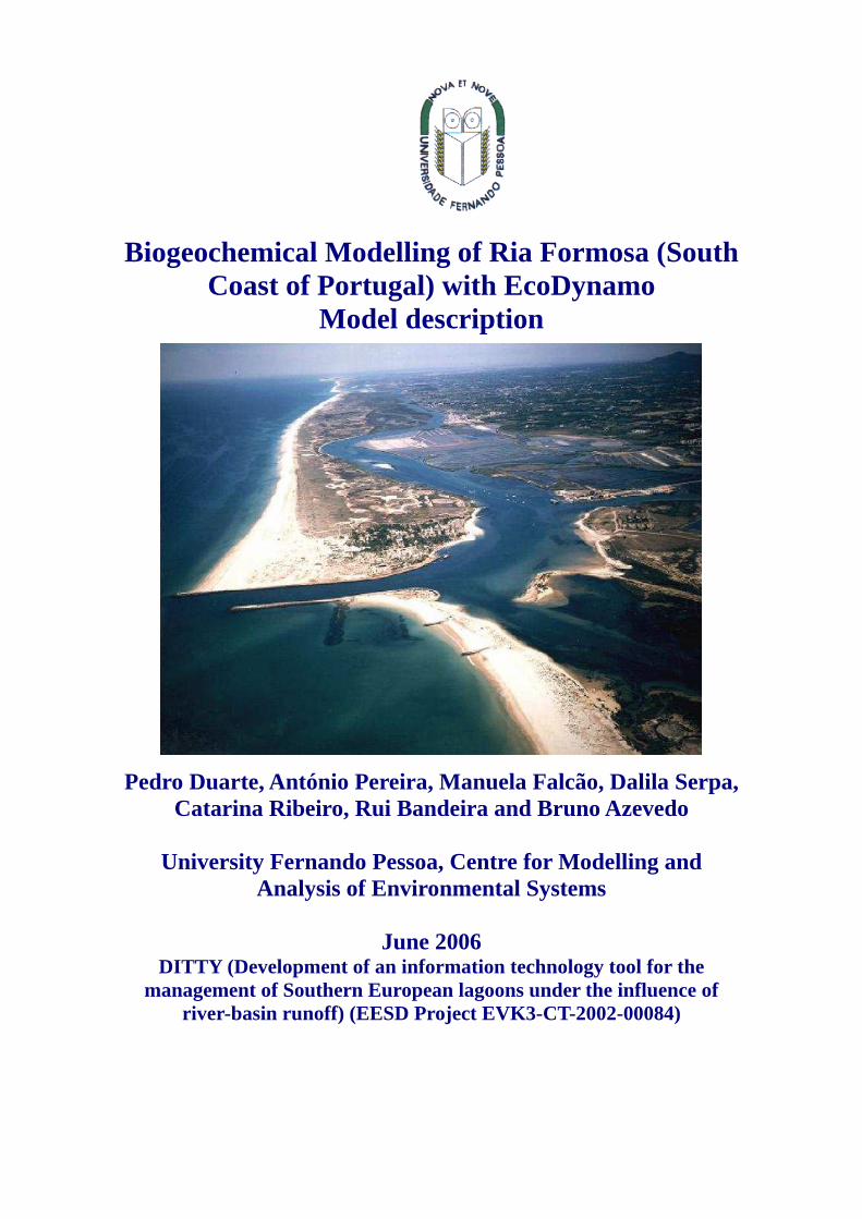
time integrated (for 5 minute periods in the present case) data series of current flows

with the hydrodynamic object, to transport water properties among model grid cells.

This allows for a faster simulation, avoiding the computation overhead of

hydrodynamic processes and the small time steps generally required. This simplified

mode was used in the present work. Whereas “online coupling” needs a 3 s time step for

stability restrictions, mostly because of very low depths over intertidal areas, the offline

simulations may use a time step of up to 60 s. In fact, a variable time step is used, so

that sites where instabilities may arise are resolved with more detail and properly time

integrated with neighbour cells. Instabilities generally occur when the volume in a cell

is very low. In this case, if the time step is not small enough, the computed flow across

one of the cell “walls” times the time step, may be larger than cell volume. When

calculating transport of salt or any other property, this situation may lead to the violation

of mass conservation. The algorithm consists in resolving with more detail these

“critical cells” and their interactions with neighbour cells, finding a time step small

enough to prevent mass conservation violations and numerical instabilities.

Regarding the multi-processing version of EcoDynamo, it handles different objects has

different threads, meaning that they may run in different processors. This implied to

synchronize the objects. The transport equation (equation 1) must be solved only after

all pelagic objects (see below) calculate their source and sink terms, because some of

these terms depend on state variables of other objects.

2.2 Biogeochemical model description

Differential equations used for suspended matter dynamics and biogeochemical

processes are shown in Tables 2-2 – 2-5. Part of these equations (those concerning

pelagic state variables), represent the sources-sinks terms of Equation 1. The

corresponding rate equations are presented in Tables 2-6 – 2-8. Model parameters are

listed in Table 2-9.

The model includes the pelagic and the benthic compartment as well as their

interactions. Pelagic variables are water temperature and those depicted in Tables 2-2

and 2-4 – dissolved nutrients, suspended matter and phytoplankton. Benthic variables

9

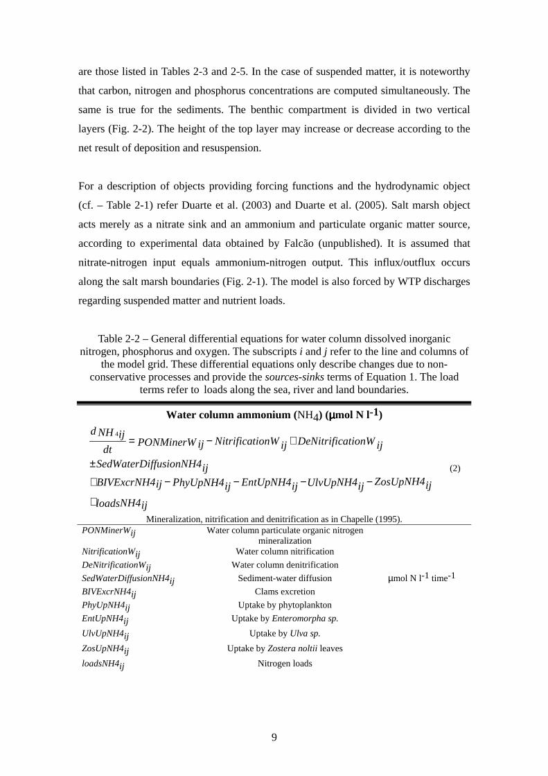
are those listed in Tables 2-3 and 2-5. In the case of suspended matter, it is noteworthy

that carbon, nitrogen and phosphorus concentrations are computed simultaneously. The

same is true for the sediments. The benthic compartment is divided in two vertical

layers (Fig. 2-2). The height of the top layer may increase or decrease according to the

net result of deposition and resuspension.

For a description of objects providing forcing functions and the hydrodynamic object

(cf. – Table 2-1) refer Duarte et al. (2003) and Duarte et al. (2005). Salt marsh object

acts merely as a nitrate sink and an ammonium and particulate organic matter source,

according to experimental data obtained by Falcão (unpublished). It is assumed that

nitrate-nitrogen input equals ammonium-nitrogen output. This influx/outflux occurs

along the salt marsh boundaries (Fig. 2-1). The model is also forced by WTP discharges

regarding suspended matter and nutrient loads.

Table 2-2 – General differential equations for water column dissolved inorganic nitrogen, phosphorus and oxygen. The subscripts i and j refer to the line and columns of

the model grid. These differential equations only describe changes due to non-conservative processes and provide the sources-sinks terms of Equation 1. The load

terms refer to loads along the sea, river and land boundaries.

Water column ammonium (NH4) (µµµµmol N l-1)

4dNH ijNitrificationW DeNitrificationWPONMinerWij ij ijdt

SedWaterDiffusionNH4ijZ NH4osUpP EntUpNH4 NH4BIVExcrNH4 hyUpNH4 UlvUpij ijij ij ij

NH4loads ij

= − +

±

− − − −+

+

(2)

Mineralization, nitrification and denitrification as in Chapelle (1995). PONMinerWij Water column particulate organic nitrogen

mineralization NitrificationWij Water column nitrification

DeNitrificationWij Water column denitrification

SedWaterDiffusionNH4ij Sediment-water diffusion

BIVExcrNH4ij Clams excretion

PhyUpNH4ij Uptake by phytoplankton

EntUpNH4ij Uptake by Enteromorpha sp.

UlvUpNH4ij Uptake by Ulva sp.

ZosUpNH4ij Uptake by Zostera noltii leaves

loadsNH4ij Nitrogen loads

µmol N l-1 time-1

10

Water column nitrate+nitrite ( NO) (µµµµmol N l-1) dNOij

NitrificationW DenitrificationW SedWaterDiffusionNOij ij ijdtZ NOosUpP EntUpNO NOhyUpNO UlvUp ijij ij ij

loadsNOij

= ±−

− − − −

+

(3) The fluxes for the uptakes have the same prefix as for ammonia to indicate the species or species group

responsible for each uptake. Their units are µmol N l-1 time-1.

Water column phosphate (PO4) (µµµµmol P l-1) 4dPO ij

SedWaterDiffusionPO4POPMinerWij ijdtZosUpP EntUphyUpPO4 PO4 UlvUpPO4 PO4ijij ij ij

PO4loads ij

= ±

− − − −

+ (4)

The fluxes for the uptakes have the same prefix as for ammonia and nitrate to indicate the species or

species group responsible for each uptake. Their units are µmol P l-1 time-1. POPMinerWij Water column particulate

organic phosphorus mineralization

Water column dissolved oxygen (DO) (mg O2 l-1)

( )dDOijKarSedWaterDiffusion DOsat DOij ijijdt

BIVResp P P ResphyPHOT hyij ij ij

Ent EntRespPHOTij ij

UlvRespPHOTUlv ij ij

ZosRespZosPHOTij ij

NitrificationConsW MineralizationConsWijij

= ± + −

− + −

+ −

+ −

+ −

− −

(5)

Raeration coefficient calculated as a function of wind speed as in Burns (2000). Oxygen consumption by nitrification and mineralization as in Chapelle (1995) and Chapelle et al. (2000). Kar Gas transfer/raeration coefficient time-1

DOsatij Dissolved oxygen saturation concentration mg O2 l-1

BIVRespij Bivalve respiration

PhyPHOTij Phytoplankton photosynthesis

PhyRespij Phytoplankton respiration

EntPHOTij Enteromorpha sp. photosynthesis

EntRespij Enteromorpha sp. respiration

UlvPHOTij Ulva sp. photosynthesis

UlvRespij Ulva sp. respiration

ZosPHOTij Zostera noltii photosynthesis

ZosRespij Z. noltii above ground respiration

NitrificationConsWij Consumption by water column nitrification

MineralizationConsWij Consumption by water column mineralization

mg O2 l-1time -1

11

Table 2-3 - General differential equations for pore water variables – pore water

ammonium, nitrate+nitrite, phosphate and oxygen – and sediment variables – organic carbon, nitrogen and phosphorus. The subscripts i and j refer to the line and columns of

the model grid.

Pore water ammonium (NH4s) (µµµµmol N l-1)

4s OrgNMinerSd SedWaterRatioNH ijij ijNitrificationS DeNitrificationSij ijdt NAtomicMass

Z RootNH4os SijSedWaterDiffusionNH4ij

= − +

−±

(6) OrgNMinerSij Mineralization of sediment organic nitrogen µg g-1 N time-1 SedWaterRatioij g l-1 NitrificationSij Pore water nitrification

DeNitrificationSij Pore water denitrification

SedWaterDiffusionNH4ij Sediment-water diffusion

ZosRootUpNH4Ssij Uptake by Zostera noltii roots

µmol N l-1 time-1

Pore water nitrate+nitrite (NOs) (µµµµmol N l-1) dNOsij

NitrificationS SedWaterDiffusionNOs DenitrificationSij ij ijdt= ± −

(7)

Nitrification and denitrification as in Chapelle (1995).

Pore water phosphate (PO4s) (µµµµmol N l-1)

4s OrgPMinerSd SedWaterRatioPO ijij ijSedWaterDiffusionijdt PAtomicMass

SedimentAdsorption SedimentDesorption ZosRootUpPO4Sij ijij

= ±

− + −

(8) Adorption and desorption as in Chapelle (1995).

OrgPMinerSij Mineralization of sediment organic phosphorus µg g-1 N time-1 ZosRootUpNH4Ssij Uptake by Z. noltii roots µmol P l-1 time-1

Pore water oxygen (DO) (mg l-1) dDOij

Zos RespSedWaterDiffusion Root ijijdtNitrificationConsS MineralizationConsSijij

−= ±

− − (9)

ZosRootRespij Z. noltii below ground respiration

NitrificationConsSij Consumption by pore water nitrification

MineralizationConsSij Consumption by pore water mineralization

mg O2 l-1time -1

12

OrgN (µµµµg N g-1) dOrgNij

DetrDepN PhySetN OrgNMinerSij ij ijdt= + − (10)

DetrDepNij Deposition of particulate nitrogen

PhySetNij Settling of phytoplankton cells

µg N g-1 time-1

OrgP(µµµµg P g-1) dOrgPij

DetrDepP PhySetP OrgPMinerSij ij ijdt= + − (11)

DetrDepPij Deposition of particulate nitrogen

PhySetPij Settling of phytoplankton cells

µg P g-1 time-1

Adsorbed PO4 (µµµµg P g-1)

( )4AdsdPO PAtomicMassijSedimentAdsorption SedimentDesorptionij ijdt SedWaterRatioij

= − (12)

(µg P g-1 time-1)

Table 2-4 – General differential equations for suspended matter. The subscripts i and j refer to the line and columns of the model grid. These differential equations only

describe changes due to non-conservative processes and provide the sources-sinks terms of Equation 1. The load terms refer to loads along the sea and river boundaries.

Total (TPM) and organic (POM) particulate matter (mg l-1) dTPMij

TPMDep TPMResus PHYTONPP POMMiner TPMLoadsij ij ij ijijdt= − + − +

(13) dPOMij

POMDep POMResus PHYTONPP POMMiner POMLoadsij ij ij ijijdt= − + − +

(14) (following Duarte et al. (2003))

TPMDepij TPM Deposition rate

TPMResusij TPM Resuspension rate

PHYTONPPij Net Phytoplankton Production (in dry weight)

TPMLoadsij TPM loads

POMDepij POM Deposition rate

POMResusij POM Resuspension rate

POMMinerij POM mineralization

POMLoadsij POM loads

mg l-1 time-1

* - POM and POM fluxes are expressed in POM mass, Carbon, Nitrogen and Phosphorus units

13

Phytoplankton (µµµµg C l-1)*

( ) -dPHYij

PHYRespPHYGPP PHYExud PHYMortPHYij ij ij ijijdtBIV convGb PHYLoadsij ijij

= − − −

+ (15)

*For output, phytoplankton biomass is converted to Chlorophyll, assuming a Chlrophyll / Carbon ratio of 0.02 (Jørgensen et al., 1991)

PHYGPPij Gross primary productivity

PHYExudij Exudation rate

PHYRespij Respiration rate

PHYMortij Mortality rate

Gbij Bivalve grazing rate

time-1

BIVijconv Bivalve biomass converted to carbon

PHYLoadsij Phytoplankton loads

µg C l-1time-1

Table 2-5 - General differential equations for benthic variables. The subscripts i and j refer to the line and columns of the model grid.

Enteromorpha sp(g DW m-2)

( )dENTij

ENTRespENT ENTGPP ENTMortij ij ijijdt= − − (18)

ENTGPPij Gross primary productivity g DW m-2 time-1

ENTRespij Respiration rate time-1

ENTMortij Mortality rate time-1

Ulva sp. (g DW m-2)

( )dULVij

ULVRespULV ULVGPP ULVMortij ij ijijdt= − − (19)

ULVGPPij Gross primary productivity g DW m-2 time-1

ULVRespij Respiration rate time-1

ULVMortij Mortality rate time-1

Zostera noltii (g DW m-2) Variables and equations as described in Plus et al. (2003)

Ruditapes decussatus (g DW m-2)

( )dBIVBij

BIVRespBIVDens BIVAbsor BIVExcr BIVMortij ij ij ijijdt= − − − (20)

dBIVDensijBIVDens BIVSeed BIVHarvij ij ijdt

= −µ + − (21)

BIVDensij Density ind. m-2 BIVAbsorij Absorption rate BIVRespij Respiration rate BIVExcrij Excretion rate BIVMortij Mortality rate

g DW ind-1 time-1

14

BIVSeedij Seeding rate BIVHarvij Harvest rate

g DW m-2 time-1

µ Mortality rate time-1

Table 2-6 – Equations for suspended matter rate processes (see text).

TPM and POM

TPMijTPMDep SinkingVelocityij ij Depthij

=

(22)

( )

( )( )

.

0

20.02 1.0,2

min 2

1.02

VelocityShearErateTPMResusij ij

if Drag CurrentVelocity CritSpeed then

elseVelocityShearij

CritSpeedVelocityShearij

Drag CurrentVelocity

CritSpeed

=

<=

−

= −

0.02 – Threshold value to avoid very high resuspension rates (calibrated)

(23)

(24)

POMijPOMDep TPMDepij ij TPMij

=

(25)

POMijPOMResus TPMResusij ij

TPMij=

(26)

2

1 3gnDrag

Depth= (calculated by the hydrodynamic object)

(27)

n Manning coefficient

g Gravity m s-2

CritSpeed Velocity threshold for resuspension m s-1

15

Table 2-7 – Equations for phytoplankton rate processes. Each rate is multiplied by corresponding carbon, nitrogen or phosphorus stocks to obtain fluxes (see text).

Processes Equations Units

Vertically integrated ( light limited productivity, from Steele’s equation (Steele, 1962))

exp 0II zexp expP Pg(I) max k z I Iopt opt

= − − −

(28)

where, Pmax – Maximum rate of photosynthesis; Iopt – Optimal light intensity for photosynthesis;

Iz – Light intensity at depth z;

time-1

Light intensity at box depth

exp( )kzI Iz 0= − (29)

µ E m-2 time-1

Light extinction coefficient

0.0243 0.0484k TPM= + (30) (empirical relationship with TPM concentration used in Duarte et al.

(2003)) m-1

Light and temperature limited productivity

.P P Tlimitg(I,T) g( )I= (31)

where, Tlimit – Temperature limitation factor

time-1

Light, temperature and nutrient limited productivity

min ,

Ncell Pcell

P T,NutPHYGPP g(I, )ij

Ncell Pcellij ijP Tg(I, )

k Ncell k Pcellij ij

= =

+ +

(32)

where, KNcell – Half saturation constant for growth limited by nitrogen cell

quota; KPcell – Half saturation constant for growth limited by phosphorus

cell quota.

time-1

Nitrogen cell quota

PHYNijNcellij

PHYCij= (33)

where, PHYNij and PHYCij represent phytoplankton biomass in nitrogen

and carbon units, respectively

mg N mg C-1

Phosphorus cell quota

PHYPijPcellij

PHYCij= (34)

where, PHYPij represent phytoplankton biomass in phosphorus units

mg P mg C-1

Nitrogen uptake

.NPHYUptakeN V PHYNijij = (35)

µg N L-1 time-

1 Phosphorus uptake

.PPHYUptakeP V PHYPijij = (36)

µg P L-1 time-1

16

Nitrogen uptake rate (VN)

If Nmin < PHYNij < Nmax and

PHYNij / PHYPij < maxN/Pij

4

4

1maxAmmonium

NH Ncellij ijV VAmmonium N Nmaxk NH ij

= − +

(37)

( ).max 0, max

1Nitrate Nitrite

V Nitrate Nitrite V VAmmoniumN

NO Ncellij ijNmaxk NOij+

−+ =

− +

(38)

NV V VAmmonium Nitrate Nitrite= + +

else VN = 0, (39)

where

Nmin – minimal nitrogen cell quota (mg N mg C-1) ;

Nmax - maximal nitrogen cell quota (mg N mg C-1) ; KAmmonium – half saturation constant for ammonium uptake

(µmol N L-1); maxN/Pij – Maximal cellular nitrogen:phosphorus ratio;

VmaxN– Maximal uptake rate (d-1);

KNitrate+Nitrite – half saturation constant for Nitrate + Nitrite

uptake (µmol N L-1);

time-1

Phosphorus uptake rate (VP)

If PHOSmin < PHYPij < PHOSmax and

PHYNij / PHYPij > minN/Pij

4

4

1maxPP

PO Pcellij ijV V P PHOSmaxk PO ij

= − +

(40) else

VP = 0, where

PHOSmin – minimal phosphous cell quota (mg P mg C-1) ;

PHOSmax - maximal phosphous cell quota (mg P mg C-1) ;

Kp – half saturation constant for phosphous uptake (µmol P L-1); minN/Pij – Minimal cellular nitrogen:phosphorus ratio;

VmaxP– Maximal uptake rate (d-1);

time-1

Phytoplankton exudation rate of Carbon

.ExudPHYGPPPHYExud ijij = , where (41)

Exud – Fraction exudated;

time-1

( )0 . . .

. .24

dark Tlimit DailyMeanPHYResp GPPR R ijij

CarbonToOxygenOxygenMolecularWeight

ChlorophyllToCarbon

= +

(42)

during the night

( )0 . . . .

. .24

dark Tlimit DLratio DailyMeanPHYResp GPPR R ijij

CarbonToOxygenOxygenMolecularWeight

ChlorophyllToCarbon

= +

17

Phytoplankton respiration rate

(43)

during the day, where

R0 – Maintenance respiration (mmol O2 mg Chl-1 h-1);

Rdark– Linear coefficient of increase in biomass-specific dark

respiration with gross photosynthesis (dimensionless);

DLratio – Ratio between respiration in the light and respiration in the dark (dimensionless);

DailyMeanGPPij - Daily integrated gross productivity (mmol

O2 mg Chl-1 h-1);

CarbonToOxygen – Conversion factor between oxygen consumed

and carbon produced in respiration (mg C mg O2-1);

ChlorophyllToCarbon – Conversion factor from chlorophyll to

carbon (mg C mg Chl-1)

time-1

Temperature limitation factor

( )( )exp TempAugRate 0Tlimit T Tij= − (44)

where,

TempAugRate – Temperature augmentation rate;

T0 – Reference temperature.

dimensionless

Nitrogen mortality loss

.. NcellPHYCPHYMortN PHYMort ijij ij ij= (45) µg N l-1time-1

Phosphorus mortality loss

.. PcellPHYCPHYMortP PHYMort ijij ij ij= (46) µg P l-1time-1

Carbon settling loss rate

SettlingSpeedPHYSetij Depthij

= , (47)

where,

SettlingSpeed – Fall velocity of phytoplankton cells (m d-1);

Depthij – Depth of layer j in column i (m)

time-1

Nitrogen settling loss

.PHYNij

SettlingSpeedPHYSetNij Depthij= (48) µg N l-1time-1

Phosphorus settling loss

.PHYPij

SettlingSpeedPHYSetPij Depthij= (49) µg P l-1time-1

18

Table 2-8 – Equations for Enteromorpha sp. and Ulva sp. rate processes. Each rate is multiplied by corresponding dry weight, carbon, nitrogen or phosphorus stocks to obtain

fluxes (see text).

Processes Equations Units

Steele’s equation (Steele, 1962))

exp 1I Iz zP Pg(I) maxI Iopt opt

= −

(50)

where, Pmax – Maximum rate of photosynthesis; Iopt – Optimal light intensity for photosynthesis;

Iz – Light intensity at depth z;

time-1

Light and temperature limited productivity

.P P Tlimitg(I,T) g( )I= (51)

where, Tlimit – Temperature limitation factor

time-1

Temperature limitation factor

( )( )1

1 exp -TempCoeff 0Tlimit

T Tij=

+ −

(52)

where,

TempCoeff – Temperature coefficient;

T0 – Reference temperature.

dimensionless

Light, temperature and nutrient limited productivity

min ,

Por T,NutENTGPP ULVGPP g(I, )ij ij

PHOSminNcell Pcellij Nmin ijP Tg(I, )

Nmax Nmin PHOSmax PHOSmin

= =

− − − −

(53)

Symbols as before for phytoplankton (cf. – Table 7)

time-1

Enteromorpha

nitrogen uptake

.NEntUpDIN V ENTijij = (54)

g N m-2 time-1

Enteromorpha

phosphorus uptake

.PEntUpDIN V ENTijij = (55)

g P m-2 time-1

Ulva nitrogen uptake

.NUlvUpDIN V ULV ijij = (56)

g N m-2 time-1 Ulva phosphorus uptake

.PUlvUpDIN V ULV ijij = (57)

g P m-2 time-1

19

Nitrogen uptake rate (VN)

4

4

max ,0maxDIN

NH NO Nmax Ncellij ij ijV VN N Nmax Nmink NH NOij ij

+ −= + + −

(58)

where KDIN – half saturation constant for inorganic nitrogen uptake

(µmol N L-1);

time -1

Phosphorus uptake rate (VP)

4

4

max ,0maxPP

PO PHOSmax Pcellij ijV V P PHOSmax PHOSmink PO ij

−= + −

(59)

time -1

Enteromorpha mortality rate

( )0,. . .

MAX OxygenDemand DOijijbetaENTDeathLoss KTEntENTMort ENT ENTij ijij OxygenDemandij

−= +

KTEnt – Mortality coefficient for oxygen limitation

OxygenDemandij – Quantity of oxygen necessary over one time step to support Enteromorpha respiration (only positive when respiration

> photosynthesis)

(60)

time -1

Ulva mortality rate

( ),0. . .

MAX OxygenDemand DOijijbetaULVDeathLoss KTUlvaULVMort ULV ULVij ijij OxygenDemandij

−= +

KTEnt – Mortality coefficient for oxygen limitation

OxygenDemandij – Quantity of oxygen necessary over one time step to support Ulva respiration (only positive when respiration >

photosynthesis)

(61)

time -1

20

Table 2-9 - Equations for Ruditapes decussatus rate processes.

Processes Equations Units

Clearance rate

WFCaCR= (62) Where,

a –allometric parameter;W – meat dry weight (g); FC – allometric exponent for clearance

L individual-1

day-1

Coefficient

WFCst

CRsta = (63)

Where, CRst – Clearance rate of a standard animal; Wst – meat dry weight of a standar clam (g)

Clearance rate of a standard clam ( ) ( ) ( )0.003 1.426 f T f DOCR TPMijst = − + (64)

L individual-1 day-1

Temperature limitation

( ) ( )

( ) ( )

20º

1.0 0.045 20.0

1.0 0.040 20.0

if CTij

f T Tij

else

f T Tij

<

= + −

= − −

(65)

(66)

Dimensionenless

Dissolved oxygen limitation

( )

( ) ( )

28%

1

1.0 0.06 28.0

if DOsatij

f DO

else

f DO DOsatij

>

=

= + −

(67)

Dimensionenless

Suspended matter filtration

.Cons CRTPMij= g individual-1 day-1

Pseudofaeces production rate

( )( )1 exp .

delta ThresCons Cons

PF PFmax xkp delta

= −

= −(68) where,

(69) ThresCons – Threshold filtration rate; PFmax – Pseudofaeces maximal production rate; xkp – Coefficient

Dimensionenless

Suspended matter ingestion

(1 )Ing Cons PF conv= − (70) g individual-1 day-1

Absorption

.A Ing AE= (71)

Where, AE – Absorption efficiency

J individual-1 day-1

(it is converted to/from g

individual-1 day-1

assuming an energy contents for the clams of 20000

J g-1 (Sobral, (1995))

Absorption efficiency

APAE AEmax

OCI= −

Dimensionless

21

Where, AEmax – Maximum absorption efficiency; AP – Empirical coefficient; OCI – Organic contents of ingested food

Respiration rate

( )Wst

W RCRstR = (72) where,

Rst – respiration of a standar mussel (1 g DW);

RC – respiration exponent

J individual-1

day-1

(it is converted to/from g

individual-1 day-1

assuming an energy contents for the clams of 20000

J g-1 (Sobral, 1995))

Respiration rate of a standard mussel

If DOsatij < 28% Rst = 1.5 else Rst = 3.1 J day-1 ind-1

22

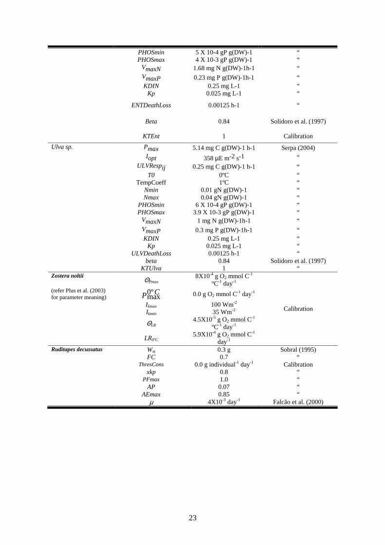
Table 2-10 – Model parameters and respective values. Most values were calibrated from ranges reported by quoted authors.

Object Parameter Value Reference

Hydrodynamic 2D object

Manning coefficient 0.03 s m-1/3 Grant and Bacher (2001)

Eddy diffusivity 5 m2 s-1 Neves (1985) Suspended matter object

CritSpeed 0.00773 m s-1 Calibrated

SinkingVelocity

0.4 and 20 m day-1 for POM and TPM,

respectively

Calibrated

Erate 432 g m-2 day-1 Calibrated Phytoplankton object Nmin 0.1 mg N mg C-1 Jørgensen et al (1991) Nmax 0.53 mg N mg C-1 “ KAmmonium 2.94 µmol N l-1 “ maxN/Pij 291 “ VmaxP and VmaxN 1.08 d-1 Cochlan & Harrison (1991) KNitrate+Nitrite 30 µmol N l-1 Jørgensen et al (1991) PHOSmin 0.002 mg P mg C-1 “ PHOSmax 0.08 mg P mg C-1 “ minN/Pij 4 “ Kp 2 µmol P l-1 “ Pmax 1.1 d-1 “ Iopt 850 µE m-2 s-1 “ KNcell 0.028 mg N mg C-1 Calibrated KPcell 0.004 mg P mg C-1 Calibrated Exud 0.1 Jørgensen et al (1991)

R0 0.02 mmol O2 mg Chl-

1 h-1

Langdon (1993)

Rdark

0.3

Calibrated

DLratio 2

Langdon (1993) CarbonToOxygen 0.3125 mg C mg O2

-1 Vollenweider (1974)

ChlorophyllToCarbon 50 mg C mg Chl-1

Jørgensen & Jørgensen (1991)

TempAugRate 0.069 ºC-1 Estimated T0 0ºC for photosynthesis

and 25ºC for respiration

Calibrated SettlingSpeed 1 m d-1 Mann & Lazier (1996)

PHYMortij 0.05 day-1 Jørgensen & Jørgensen

(1991) Enteromorpha sp Pmax 6.93 mg C g(DW)-1 h-1 Serpa (2004) Iopt 335 µE m-2 s-1 “ ENTRespij 0.04 mg C g(DW)-1 h-1 “ T0 0ºC “ TempCoeff 1ºC “ Nmin 0.01 gN g(DW)-1 “ Nmax 0.035 gN g(DW)-1 “

23

PHOSmin 5 X 10-4 gP g(DW)-1 “ PHOSmax 4 X 10-3 gP g(DW)-1 “ VmaxN 1.68 mg N g(DW)-1h-1 “ VmaxP 0.23 mg P g(DW)-1h-1 “ KDIN 0.25 mg L-1 “ Kp 0.025 mg L-1 “

ENTDeathLoss 0.00125 h-1 “

Beta 0.84 Solidoro et al. (1997)

KTEnt 1 Calibration

Ulva sp. Pmax 5.14 mg C g(DW)-1 h-1 Serpa (2004) Iopt 358 µE m-2 s-1 “ ULVRespij 0.25 mg C g(DW)-1 h-1 “ T0 0ºC “ TempCoeff 1ºC “ Nmin 0.01 gN g(DW)-1 “ Nmax 0.04 gN g(DW)-1 “ PHOSmin 6 X 10-4 gP g(DW)-1 “ PHOSmax 3.9 X 10-3 gP g(DW)-1 “ VmaxN 1 mg N g(DW)-1h-1 “ VmaxP 0.3 mg P g(DW)-1h-1 “ KDIN 0.25 mg L-1 “ Kp 0.025 mg L-1 “ ULVDeathLoss 0.00125 h-1 “ beta 0.84 Solidoro et al. (1997) KTUlva 1 “ Zostera noltii

ΘPmax 8X10-4 g O2 mmol C-1

ºC-1 day-1 (refer Plus et al. (2003) for parameter meaning)

0ºmax

CP 0.0 g O2 mmol C-1 day-1

Ikmax 100 Wm-2 Ikmin 35 Wm-2

ΘLR 4.5X10-5 g O2 mmol C-1

ºC-1 day-1

LR0ºC 5.9X10-4 g O2 mmol C-1

day-1

Calibration

Ruditapes decussatus Wst 0.3 g Sobral (1995) FC 0.7 “ ThresCons 0.0 g individual-1 day-1 Calibration xkp 0.8 “ PFmax 1.0 “ AP 0.07 “ AEmax 0.85 “ µ 4X10-3 day-1 Falcão et al. (2000)

24

2.2.1. Hydrodynamic object

The hydrodynamic object was described in a previous report (Duarte et al., 2005). This

object allows the output of time integrated current velocities and flow values for each

grid cell. These outputs may later be used to run the remaining objects without the

necessary calculation overhead of the hydrodynamic processes. Therefore, a specific

transport object was implemented in EcoDynamo just to handle the time series

calculated by the hydrodynamic object. This transport object computes the equation of

continuity, as described in Duarte et al. (2005) and the transport equation (1) for all

pelagic variables of the other objects.

2.2.2. Wind object

This object returns wind speed forcing variable average values to the water temperature

object. These values are then used to calculate water heat losses through evaporation.

2.2.3. Air temperature object

This object reads forcing variable air temperature values and returns them to the water

temperature object, to be used to calculate sensible heat exchanges between the water

and the atmosphere.

2.2.4. Light intensity and water temperature object s

Light intensity and water temperature were calculated by a light and a water

temperature object using standard formulations described in Brock (1981) and Portela &

Neves (1994). Submarine light intensity was computed from the Lambert-Beer law. The

water light extinction coefficient was computed by the suspended matter object (cf. –

2.2.6).

2.2.5 Dissolved substances object

The concentrations of dissolved inorganic nitrogen (DIN) - ammonium, nitrite and

nitrate -, inorganic phosphorus and oxygen in each of the model grid cells are calculated

25

as a function of biogeochemical and transport processes, including exchanges with the

sea, loads from rivers and waste water treatment plants (WTPs), and exchanges across

the sediment water interface (Figs. 2-1, 2-2 and Table 2-2).

These variables are also calculated in pore water (Table 2-3). Both the nitrogen and

phosphorus cycles are simulated using equations and parameters described in Chapelle

(1995). The only exception is the raeration coefficient, calculated as a function of wind

speed, following Burns (2000). Phytoplankton and macroalgae remove nutrients from

flowing water. Zostera noltti also removes nutrients from pore water through the roots

(Plus et al., 2003).

2.2.6 Suspended matter object

This object computes total particulate matter (TPM in mg L-1) and particulate organic

matter (POM in mg L-1) from deposition and resuspension rates, from the exchanges

with the sea and with other boxes (transport by the hydrodynamic object), and from the

net contribution of phytoplankton biomass (Figs. 2-1, 2-2 and Table 2-4). POM

mineralization is calculated as in Chapelle (1995), returning the resulting inorganic

nitrogen and phosphorus to the dissolved substances object.

Deposition of TPM in each grid cell is based on sinking velocity and cell depth

(returned by the hydrodynamic object). Sinking velocity is considered constant but with

different values for inorganic and organic matter (calibrated) (Tables 2-4, 2-6 and 2-10).

Resuspension of TPM in each grid cell is calculated as a function of current velocity

and bottom drag, returned by the hydrodynamic object (Table 2-6). Below a critical

velocity value, resuspension does not occur. Above a certain threshold for the product of

bottom drag times current velocity (velocity shear), resuspension is assumed constant.

This is to avoid unrealistically high resuspension rates. This object is partly based on a

Stella model developed by Grant and Bacher (unpublished).

26

The light extinction coefficient (m-1) is calculated from an empirical relationship with

TPM (Equation 30 in Table 2-7), obtained from historical data for Sungo Bay (Bacher,

pers com).

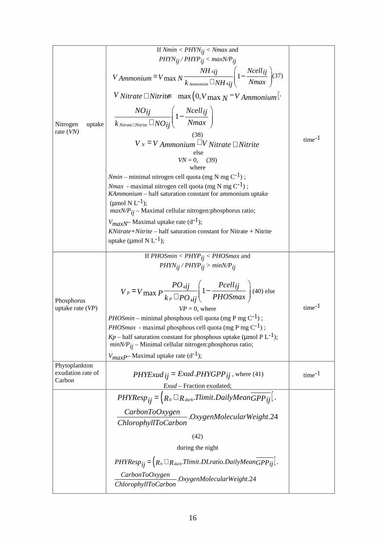
2.2.7 Phytoplankton object

Phytoplankton productivity is described as a function of light intensity (depth integrated

Steele’s equation) (Steele, 1962), temperature and a limiting nutrient – nitrogen or

phosphorus (Tables 2-4 and 2-7). In this model, phytoplankton is represented through

chlorophyll, carbon, nitrogen and phosphorus pools. This allows the necessary

bookkeeping calculations on cell quotas. Traditional approaches with models based

solely on nitrogen or phosphorus do not allow these computations. Internal cell quotas

are then used to limit carbon fixation through photosynthesis. A nutrient limiting factor

in the range 0 – 1 is calculated both for internal nitrogen and phosphorus. The lowest

obtained value is then multiplied by light and temperature limited photosynthesis

following Liebig’s law of minimum.

Nutrient uptake and limitation is described as a three-stage process (Table 2-7,

equations 35-40), following Jørgensen & Bendoricchio (2001) :

(i) The uptake of nitrogen and phosphorus is dependent on their concentration

in the water, on their cell quotas and on the ranges of their cellular ratios;

(ii) After uptake, nutrients accumulate in the cells;

(iii) Internal nutrient concentration is used to limit phytoplankton productivity.

A Michaelis-Menten equation is used to relate nutrient uptake with their concentration

in the water, following several authors (e.g. Parsons et al., 1984; Ducobu et al., 1998;

Jørgensen & Bendoriccchio, 2001). The parameters of this equation are the half-

saturation constant and the maximum uptake rate. These were taken from the literature,

within the range of measured values (Cochlan and Harrison, 1991; Jørgensen et al.,

1991). The Michaelis-Menten equation is not the only regulating mechanism of nutrient

uptake, which is also constrained by current cell quotas to avoid values outside ranges

reported in the literature. When N:P ratios are outside limits currently measured, N or P

uptake is constrained. Nitrogen uptake rate is calculated first for ammonium nitrogen

and then for nitrite + nitrate, reducing their uptake proportionally to ammonium uptake.

This is based on the usual assumption that ammonium is the preferred nitrogen source

27

for phytoplankton (Parsons et al., 1984). Phytoplankton respiration is based on the

model of Langdon (1993) (Table 2-7, equations 42 and 43).

2.2.8 Enteromorpha spp. and Ulva spp. objects

These objects were computed as described in Solidoro et al. (1997) and Serpa (2004)

(Tables 2-5 and 2-8).

2.2.9 Zostera noltii object

This object computes Z. noltii photosynthesis, respiration, nutrient uptake, translocation

and reclamation, growth, mortality and recruitment as described in Plus et al. (2003),

except for some modifications described below. In Plus et al. (2003), growth is

calculated without considering any limit to plant individual weight or size. Therefore,

the model may produce biomass standing stocks and plant densities that imply

unrealistically large individual sizes. This can be avoided by careful calibration.

However, in the present model it was decided to create some mechanisms to avoid this

potential problem. This was done by defining an asymptotic individual weight for

Zostera leaves. Any biomass production leading to growth above that asymptotic value

is released as detritus to the suspended matter object. Z. noltii parameters differing from

those reported in Plus et al. (2003) are listed in Table 2-10, using the same symbols of

those authors.

2.2.10 Ruditapes decussatus object

Differential and rate equations for the clam object are depicted in Tables 2-5 and 2-9,

respectively. Parameters are listed in Table 2-10. Rate equations were obtained from

ecophysiology data reported in Sobral (1995). The general approach to simulate bivalve

feeding and growth is similar to other works (e.g. Raillard et al., 1993; Raillard &

Ménesguen, 1994; Ferreira et al., 1998; Duarte et al., 2003). Clearance rate is computed

from an empirical relationship with TPM, water temperature and oxygen concentration.

Temperature limitation is calculated from a direct linear relationship with water

temperature, until 20ºC, and an inverse linear relationship, above that value. Oxygen

28

limitation is calculated as a linear function of oxygen saturation, when this is below

28% saturation (hypoxia conditions). Ingestion is calculated from clearance and

pseudofaeces production rate. Absorption is calculated from ingestion and faeces

production and the usual asymptotic relationship with ingested organics (e.g. Hawkins

et al., 1998). Scope for growth is calculated from absorption and metabolism.

Respiration is calculated as a function of oxygen saturation. When saturation is below

33 %, respiration rate decreases (Sobral, 1995). Allometric relationships are used to

correct for bivalve weight.

2.3 Model setup

In what concerns pelagic variables, the model was initialized with the same

concentrations over all model domain, under the assumption that local and exchange

processes would produce a rapid change (within a few hours) of initial conditions,

which was the case. Regarding pore water and sediment variables, uniform values were

used to initialize conditions in similar sediment types. These were defined as sand,

sand-muddy, muddy-sand and muddy. Water, pore water and sediment variable values

were obtained from a database available at the DITTY project web site

(www.dittyproject.org). Sediment types and distribution of benthic variables were

obtained from a GIS developed partly during the DITTY project (Rodrigues et al.,

2005). Figs 2-4 – 2-6 summarize distribution of sediment types and benthic variables.

Fig. 2-4 – GIS image showing sediments type distribution in Ria Formosa.

29

Enteromorpha spSalt Marsh

Ulva sp. Zoostera noltii

Enteromorpha spSalt Marsh

Ulva sp. Zoostera noltii

Enteromorpha spSalt Marsh

Ulva sp. Zoostera noltii

Salt Marsh

Ulva sp. Zoostera noltii

Fig. 2-5 – GIS images showing Ria Formosa benthic species considered in this work – Salt Marshes, Ulva sp., Enteromorpha sp and Zostera noltti.

30

Fig. 2-6 – Ria Formosa shellfish farming areas.

31

2.4 Model testing

Validation of the hydrodynamic sub-model was carried out before (Duarte et al., 2005;

Duarte et al, submitted) and will not be discussed in this work. The same applies to the

SWAT model application used to force the lagoon model at river boundaries (Guerreiro

& Martins, 2005).

Regarding the biogeochemical sub-model, a significant part of model parameters was

taken from the literature: e.g. water column and sediment biogeochemistry, seagrass,

macroalgal and some phytoplankton parameters from Chapelle (1995), Solidoro et al.

(1997), Plus et al. (2003), Serpa (2004) and Falcão (1996), respectively. Some

parameters were calibrated with a zero dimensional (0D) version of the model. Several

simulations were carried out with full model complexity to check if predictions

remained within reasonable limits.

For the purposes of model calibration and validation it is important to have data on

boundary and forcing conditions collected simultaneously with data inside the lagoon.

Most of the data available for Ria Formosa does not fulfil these requirements – for some

years there is data collected inside the lagoon but not at the sea and river boundaries and

vive-versa. Fortunately, there is a relatively old data set for 1992 (Falcão, 1996) that

includes nutrient data inside and outside (at the sea boundary) the lagoon sampled at a

number of stations depicted in Fig 2-3. This data set was used to test the model. This

test simulation will be hereafter referred as the “standard simulation”. However, given

the fact that lagoon bathymetry changes very rapidly and that the bathymetry used in the

model was obtained in a relatively recent survey (conducted by the Portuguese

Hydrographic Institute in 2000), the comparison between observed and predicted data

should be carried out with caution.

32

3 Results and discussion

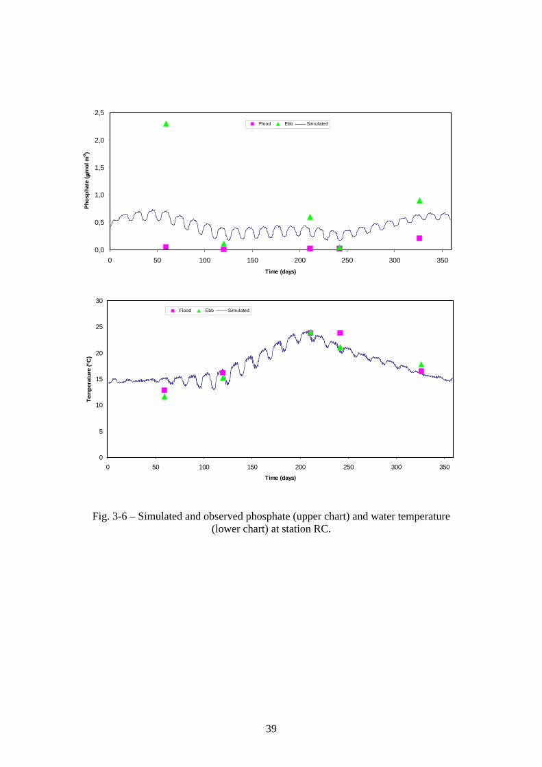
Comparisons between observed and predicted values in the Standard simulation (cf. –

Methodology – Model testing) are shown in Figs. 3-1 to 3-6 for nitrate, ammonia,

phosphate and water temperature. Observations were made during the ebb and during

the flood for each sampling occasion. Nutrient flood values are lower than ebb values

and closer to the sea boundary conditions, except for nitrate in some occasions. This is

also the case for simulated data, as can be seen for nitrate in Fig. 3-1, shown together

with water depth. The small number of observations prevents any powerful statistical

test to quantify model performance. Furthermore, data is available only for a small

number of stations located not very distant from one another (c.a. 500 – 1000 m) and for

a small number of variables. However, in most situations, the ranges predicted by the

model are within those observed, with the poorer performance for ammonia -

overestimated by the model.

Fig. 3-7 shows an example of two contour plots – for nitrate and chlorophyll. The range

for nitrate is very large (up to 880 µmol L-1) as a result of river inputs. Apart from river

mouths, concentrations are usually around 1 µmol L-1.

Comparisons between model predictions and ranges reported in several works were also

made for the biomass of benthic species, water column chlorophyll, sediment pore

water nutrient and oxygen concentrations and sediment carbon, nitrogen and

phosphorus contents. However, available data for these variables were obtained in

different years than water quality data shown in Figs. 3-1 – 3-6. Therefore, comparisons

with results reported in other authors (Aníbal, 1998; Falcão et al., 2000; Santos et al.,

2000) were just to make sure that model predictions remained within reasonable limits,

which was the case.

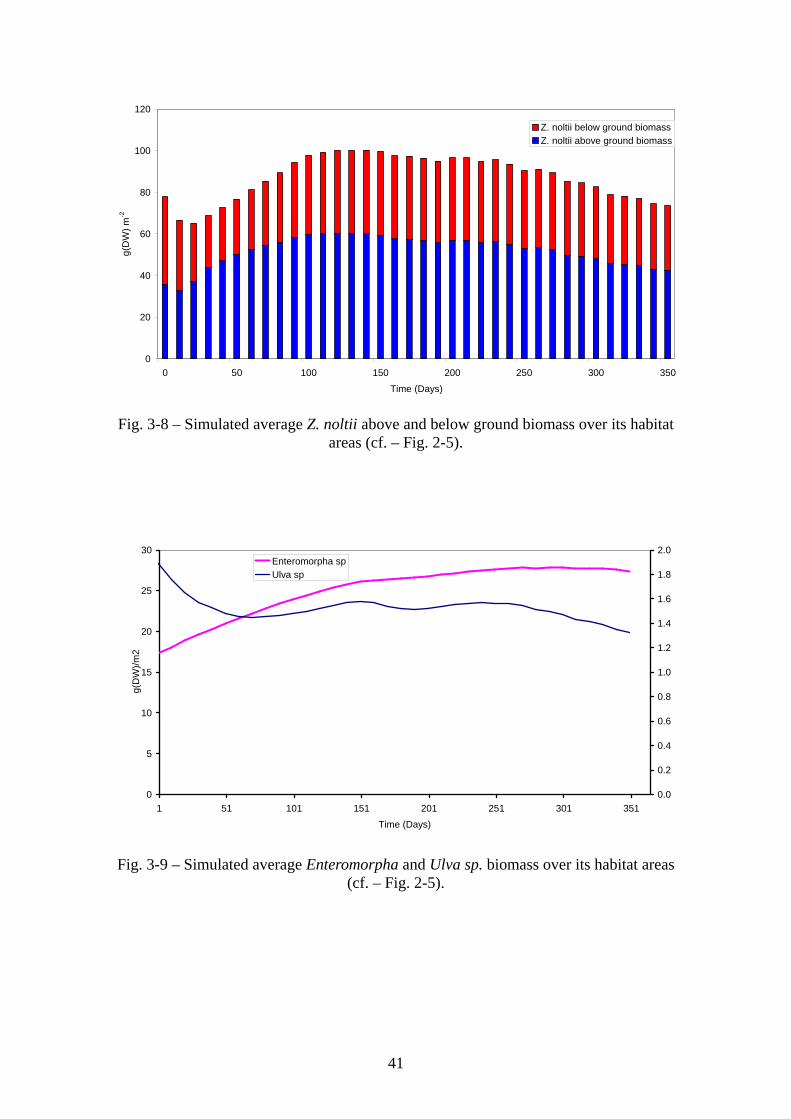
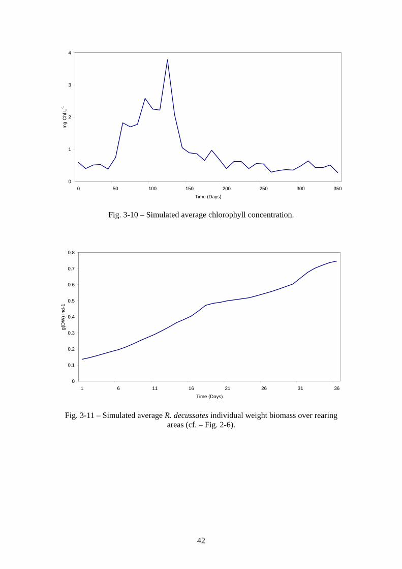
Figs. 3-8 – 3-10 show predicted average Z. noltii, Enteromorpha sp., Ulva sp. biomasses

and chlorophyll concentrations over a period of one year. The model may underestimate

Z. noltii biomass, which has been reported to reach values in excess of 200 g (DW) m-2

is some areas, without a very clear seasonal pattern (Santos et al., 2000). However,

considering that the results shown in Fig. 3-8 are averages over all habitat area (cf. –

33

Fig. 2-5), this underestimation is probably not very large. In what concerns macroalgae,

Enteromorpha and Ulva biomasses hardly reach 50 and 10 g (DW) m-2, respectively,

with the latter being usually below 5 g (DW) m-2 (Aníbal, 1998). Fig 3-11 shows R.

decussatus average individual weight for the same period. Clam growth is similar to

growth curves reported in previous works (Falcão et al., 2000).

Table 3-1 synthesis average values predicted by the model for a period of one year for

several sediment and pore water variables, considering the sediment types depicted in

Fig. 2-4. All values are well within ranges measured in Ria Formosa at the different

sediment types as checked in a database available at the DITTY web site.

Although presented results do not allow a complete and systematic testing of the model

in the light of available data, due to the lack of a complete dataset for one year,

including boundary conditions, the model, as it is, seems to be a good starting point as a

management tool. Further testing is necessary and also several improvements in the

definition of initial conditions. For example, GIS data presented in Fig. 2-5 are only an

approximate representation of the distribution of macroalgae and seagrasses.

Furthermore, the functional role of salt marshes in Ria Formosa need to be accessed to

improve their forcing to the model.

34

Fig 3-1- Simulated and observed nitrate (upper chart) and ammonia (lower chart) at station RA. Also shown simulated box depth to emphasize the opposite trends between

concentration and water depth (upper chart)

0.0

0.5

1.0

1.5

0 50 100 150 200 250 300 350

Time (days)

Nitr

ate

(µµ µµm

ol m

-3)

0.0

1.0

2.0

3.0

4.0

5.0

6.0

7.0

8.0

9.0

10.0

Depht (m

)Flood Ebb Box Depth Simulated

0.0

1.0

2.0

3.0

4.0

5.0

6.0

0 50 100 150 200 250 300 350

Time (days)

Am

mon

ium

(mm

ol m

-3)

Flood Ebb Simulated

35

Fig 3-2- Simulated and observed phosphate (upper chart) and water temperature (lower chart) at station RA.

0,0

0,5

1,0

1,5

2,0

2,5

0 50 100 150 200 250 300 350

Time (days)

Pho

spha

te (

µµ µµmol

m-3

)Flood Ebb Simulated

0

5

10

15

20

25

30

0 50 100 150 200 250 300 350

Time (days)

Tem

pera

ture

(ºC

)

Flood Ebb Simulated

36

Fig. 3-3 – Simulated and observed nitrate (upper chart) and ammonia (lower chart) at station RB.

0,0

0,5

1,0

1,5

2,0

2,5

3,0

0 50 100 150 200 250 300 350

Time (days)

Nitr

ate

(µµ µµm

ol m

-3)

Flood Ebb Simulated

0,0

1,0

2,0

3,0

4,0

5,0

6,0

7,0

8,0

0 50 100 150 200 250 300 350

Time (days)

Am

mon

ium

(µµ µµm

ol m

-3)

Flood Ebb Simulated

37

Fig. 3-4 – Simulated and observed phosphate (upper chart) and water temperature (lower chart) at station RB.

0,0

0,5

1,0

1,5

2,0

2,5

3,0

0 50 100 150 200 250 300 350

Time (days)

Pho

spha

te (

µµ µµmol

m-3

)Flood Ebb Simulated

0

5

10

15

20

25

30

0 50 100 150 200 250 300 350

Time (days)

Tem

pera

ture

(ºC

)

Flood Ebb Simulated

38

Fig. 3-5 – Simulated and observed nitrate (upper chart) and ammonia (lower chart) at station RC.

0,0

0,5

1,0

1,5

2,0

2,5

3,0

3,5

0 50 100 150 200 250 300 350

Time (days)

Nitr

ate

(µµ µµm

ol m

-3)

Flood Ebb Simulated

0,0

0,5

1,0

1,5

2,0

2,5

3,0

3,5

4,0

4,5

5,0

0 50 100 150 200 250 300 350

Time (days)

Am

mon

ium

(µµ µµm

ol m

-3)

Flood Ebb Simulated

39

Fig. 3-6 – Simulated and observed phosphate (upper chart) and water temperature (lower chart) at station RC.

0,0

0,5

1,0

1,5

2,0

2,5

0 50 100 150 200 250 300 350

Time (days)

Pho

spha

te (

µµ µµmol

m-3

)

Flood Ebb Simulated

0

5

10

15

20

25

30

0 50 100 150 200 250 300 350

Time (days)

Tem

pera

ture

(ºC

)

Flood Ebb Simulated

40

Fig. 3-7 – Example of contour plots showing nitrate (upper figure) in µmol L-1 and chlorophyll concentrations (lower figure) in µg L-1.

41

0

20

40

60

80

100

120

0 50 100 150 200 250 300 350

Time (Days)

g(D

W)

m-2

Z. noltii below ground biomassZ. noltii above ground biomass

Fig. 3-8 – Simulated average Z. noltii above and below ground biomass over its habitat areas (cf. – Fig. 2-5).

0

5

10

15

20

25

30

1 51 101 151 201 251 301 351

Time (Days)

g(D

W)/

m2

0.0

0.2

0.4

0.6

0.8

1.0

1.2

1.4

1.6

1.8

2.0Enteromorpha spUlva sp

Fig. 3-9 – Simulated average Enteromorpha and Ulva sp. biomass over its habitat areas (cf. – Fig. 2-5).

42

0

1

2

3

4

0 50 100 150 200 250 300 350

Time (Days)

mg

Chl

L-1

Fig. 3-10 – Simulated average chlorophyll concentration.

0

0.1

0.2

0.3

0.4

0.5

0.6

0.7

0.8

1 6 11 16 21 26 31 36

Time (Days)

g(D

W)

ind-

1

Fig. 3-11 – Simulated average R. decussates individual weight biomass over rearing areas (cf. – Fig. 2-6).

43

Table 3-1 – Sediment and pore water average values (0 – 5 cm), predicted by the model for different sediment types over a period of one year.

Organic carbon

Organic nitrogen

Organic phosphorus

Adsorbed phosphorus Ammonium Nitrate Phosphate

µµµµg g-1 µµµµmol L -1 Mud 7951.85 366.59 161.88 2.80 38.67 0.85 0.95 Muddy-sand 5268.89 192.51 66.87 1.72 39.94 0.81 1.67 Sany-mud 5254.10 175.98 65.01 1.76 39.75 0.93 1.76 Sand 2851.39 76.38 20.53 2.38 33.53 0.43 1.58

44

4 References Aníbal, J., 1998. Impacte da macroepifauna sobre as macroalgas Ulvales (Chlorophyta)

na Ria Formosa. MSc Thesis. Coimbra University, 73 pp.

Brock, T.D., 1981. Calculating solar radiation for ecological studies. Ecol Modelling 14, 1 - 9. Burns, L.A., 2000. Exposure analysis modelling system (EXAMS): User manual and system documentation. U.S. Environmental Protection Agency. Chapelle, A., 1995. A preliminary model of nutrient cycling in sediments of a Mediterranean lagoon. Ecological Modelling 80: 131-147. Chapelle, A., Ménesguen, A., Deslous-Paoli, J.M., Souchu, P., Mazouni, N., Vaquer, A. and B. Millet, 2000. Modelling nitrogen, primary production and oxygen in a Mediterranean lagoon. Impact of oysters farming and inputs from the watershed. Ecological Modelling 127: 161-181. Cochlan, W. P. & P.J. Harrison, 1991. Uptake of nitrate, ammonium, and urea by nitrogens-starved cultures of Micromonas pusilla (Prasinophyceae): transient esponses. J. Phycol.: 673-679. Duarte, P., Meneses, R. , Hawkins, A.J.S., Zhu, M., Fang, J. and J. Grant, 2003. Mathematical modelling to assess the carrying capacity for multi-species culture within coastal water. Ecological Modelling 168: 109-143. Duarte, P., Azevedo, B. and A. Pereira, 2005. Hydrodynamic Modelling of Ria Formosa (South Coast of Portugal) with EcoDynamo. DITTY report. Available at http://www.dittyproject.org/Reports.asp. Ducobu, H., Huisman, J., Richard, Jonker, R. & L.R. Mur, 1998. Competition between a Prochlorophyte and a Cyanobacterium under various phosphorus regimes: comparison with the droop model. Journal of Phycology: 467-476. Falcão, M.M., 1996. Dinâmica dos nutrientes na Ria Formosa: efeitos da interacção da laguna com as suas interfaces na reciclagem do azoto, fósforo e sílica. PhD, University of Algarve. Falcão, M, Duarte, P., Matias, D., Joaquim, S., Fontes, T. & R. Meneses, 2000. Gestão do cultivo de bivalves na Ria Formosa com recurso à modelação matemática. IPIMAR. Falcão, M, L. Fonseca, D. Serpa, D. Matias, S. Joaquim, P. Duarte, A. Pereira, C. Martins & M.J. Guerreiro, 2003. Synthesis report. Available at http://www.dittyproject.org/Reports.asp.

45

Ferreira, J., Duarte, P. & B. Ball, 1998. Trophic capacity of Carlingford Lough for aquaculture - analysis by ecological modelling. Aquatic Ecology, 31 (4): 361 – 379. Grant, J., & C. Bacher, 2001. A numerical model of flow modification induced by suspended aquaculture in a Chinese Bay. Can. J. Fish. Aquat. Sci. 58: 1 - 9. Guerreiro, M.J. & C. Martins, 2005. Calibration of SWAT Model: Ria Formosa Basin (South Coast of Portugal). DITTY report. Available at http://www.dittyproject.org/Reports.asp. Hawkins, A. J. S., Bayne, B.L., Bougrier, S., Héral, M., Iglesias, J.I.P., Navaro, E., Smith, R.F.M. & M.B. Urrutia, 1998. Some general relationships in comparing the feeding physiology of suspension-feeding bivalve molluscs. Journal of Experimental Marine Biology and Ecology 219: 87-103. Jørgensen, S.E. & G. Bendoricchio, 2001. Fundamentals of ecological modelling. Developments in Ecological Modelling 21. Elsevier, Amsterdam, 530 pp. Jørgensen, S.E., Nielsen, S. & L. Jørgensen, 1991. Handbook of Ecological Parameters and Ecotoxicology. Elsevier, Amsterdam, 1263 pp. Knauss, J.A. 1997. Introduction to physical oceanography. Prentice-Hall. Langdon, C., 1993. The significance of respiration in production measurements based on oxygen. ICES mar. Sci. Symp. 197, 69-78. Mann, K.H. & J.R.M. Lazier, 1996. Dynamics of marine ecosystems. Blackwell Science. Neves, R.J.J., 1985. Étude expérimentale et modélisation mathématique des circulations transitoire et rédiduelle dans l’estuaire du Sado. Ph.D. Thesis, Université de Liège. Parsons, T.R., Takahashi, M., & B. Hargrave, 1984. Biological oceanographic processes. 3rd. Edition. Pergamon Press. Pereira, A. & P. Duarte, 2005. EcoDynamo Ecological Dynamics Model Application. University Fernando Pessoa. DITTY report. Available at http://www.dittyproject.org/Reports.asp. Plus, M., Chapelle,A., Ménesguen, A., Deslous-Paoli, J.-M. & I. Auby, 2003. Modelling seasonal dynamics of biomasses and nitrogen contents in a seagrass meadow (Zostera noltti Hornem.): application to the Thau lagoon (French Mediterranean coast). Ecological Modelling 161: 213-238. Portela, L.I. & R. Neves, 1994. Modelling temperature distribution in the shallow Tejo estuary. In: Tsakiris and Santos (Editors), Advances in Water Resources Technology and Management, Balkema, Rotterdam, pp. 457 - 463. Raillard, O., Deslous-Paoli , J.-M., Héral, M. & D. Razet , 1993. Modélisation du comportement nutritionnel et de la croissance de l'huître japonaise Crassostrea gigas.” Oceanologica Acta 16: 73-82.

46

Raillard, O. & A. Ménesguen, 1994. An ecosystem box model for estimating the carrying capacity of a macrotidal shellfish system. Marine Ecology Progress Series 115: 117-130. Rodrigues, A. Carvalho, A., Reia, J., Azevedo, B., Martins, C., Duarte, P., Serpa, D. & M. Falcão, 2005. A geographical information system for Ria Formosa (South coast of Portugal). DITTY report. Available at http://www.dittyproject.org/Reports.asp. Santos, R, Sprung, M., Machás, R., Aníbal, J., Dias, N., Mata, L., Vieira, V., Piedade, F., Pérez-Lloréns, L., Hernández, I., Vergara, J. & G. Peralta, 2000. Relatório final do projecto “Produção bentónica e fluxos de matéria orgânica na Ria Formosa, Algarve, Portugal. Relatório final do projecto contracto nº º 12/REG/6196. Serpa, D., 2004. Macroalgal (Enteromorpha spp. and Ulva spp.) primary productivity in the Ria Formosa lagoon. Master thesis, Faculty of Science and Technology, New University of Lisbon. Service Hydrographique et Océanographique de la Marine (SHOM), 1984. Table des marées des grands ports du Monde. Service Hydrographique et Océanographique de la Marine, 188 pp. Sobral, M.P.O., 1995. Ecophysiology of Ruditapes decussatus L. (Bivalvia, Veneridae). PHD thesis, Universidade Nova de Lisboa. Solidoro,C., Pecenik, G.., Pastres, R., Franco, D. & C. Dejak ,1997. Modelling macroalgae (Ulva rigida) in the Venice lagoon: Model structure identification and first parameters estimation. Ecological Modelling, 94: 191-206. Steele, J.H., 1962. Environmental control of photosynthesis in the sea. Limnol. Oceanogr., 7: 137-150. UE (2000). Directiva 2000/60/CE do Parlamento Europeu e do Conselho que estabelece um Quadro de Acção Comunitária no Domínio da Política da Água. J.O.C. de 22.12.2000. Vollenweider, R.A., 1974. A manual on methods for measuring primary productivity in aquatic environments. Blackwell Scientific Publications.