HAL Id: inria-00544387https://hal.inria.fr/inria-00544387

Submitted on 3 Feb 2011

HAL is a multi-disciplinary open accessarchive for the deposit and dissemination of sci-entific research documents, whether they are pub-lished or not. The documents may come fromteaching and research institutions in France orabroad, or from public or private research centers.

L’archive ouverte pluridisciplinaire HAL, estdestinée au dépôt et à la diffusion de documentsscientifiques de niveau recherche, publiés ou non,émanant des établissements d’enseignement et derecherche français ou étrangers, des laboratoirespublics ou privés.

Biochemical Reaction Rules with ConstraintsMathias John, Cédric Lhoussaine, Joachim Niehren, Cristian Versari

To cite this version:Mathias John, Cédric Lhoussaine, Joachim Niehren, Cristian Versari. Biochemical Reaction Ruleswith Constraints. 20th European Symposium on Programming Languages, Mar 2011, Saarbrücken,Germany. Springer, 6602, pp.338-357, 2011, LNCS. <inria-00544387>

Biochemical Reaction Rules with Constraints

Mathias John12, Cedric Lhoussaine12,Joachim Niehren13, and Cristian Versari4

1 BioComputing, Lifl (Cnrs Umr8022) & Iri (Cnrs Usr3078)2 University of Lille 1

3 Inria, Lille4 University of Bologna

Abstract. We propose React(C ), an expressive programming languagefor stochastic modeling and simulation in systems biology that is basedon biochemical reactions with constraints. We prove that React(C ) canexpress the stochastic π-calculus, in contrast to previous rule-based pro-gramming languages, and further illustrate the high expressiveness ofReact(C ). We present a stochastic simulator for React(C ) independentlyof the choice of the constraint language C . Our simulator decides for agiven reaction rule whether it can be applied to the current biochemicalsolution. We show that this decision problem is NP-complete for arbi-trary constraint systems C and that it can be solved in polynomial timefor rules of bounded arity. In practice, we propose to solve this problemby constraint programming.

1 Introduction

The paradigm of chemical reactions is predominant in programming languagesused for modeling and simulation in systems biology [6, 9, 3, 19, 1]. Chemical re-actions are advantageous in that they can be given both, a continuous semanticsin terms of ordinary differential equations (odes) as well as a stochastic seman-tics in terms of continuous time Markov chains (ctmcs). While odes describedeterministically the average dynamics of molecule populations, ctmcs describethe probabilities and speed of molecular interactions in an individual-based man-ner. The continuous semantics of a system of chemical reactions is an abstractionof its more precise stochastic semantics.

Biochemical reactions in the κ-calculus are widely accepted as a useful mod-eling language for systems biology [4, 12, 5, 6]. The underlying idea is to modelbiochemical reactions as graph rewrite rules. The following rewrite rule, for in-stance, states that a C-molecule with a free binding site 1 can be linked toan A-B complex by using the free binding site 1 of A (while the complex usesbinding sites 2 of A and 1 of B).

A(1 + 2y), B(1y), C(1)4.5−−→ (νx)A(1x + 2y), B(1y), C(1x)

The stochastic rate 4.5 determines the distribution of the speed of this interac-tions according to the law of mass-action.

The alternative paradigm of agent-based modeling languages attracted alsomuch interest for modeling and simulation in systems biology. It underlies thestochastic π-calculus and its many extensions, [18, 21, 14, 17, 23, 11], BioAmbi-ents [20], BlenX or beta-binders [22], etc. The close relationship between model-ing languages of both paradigms was first pointed out by Cardelli [2]. He iden-tified the fragment of the stochastic π-calculus without ν-binders with systemsof chemical reactions with the same ctmcs in order to obtain a continuous se-mantics of π-calculus processes in terms of odes. So far, however, there existsno positive result showing the expressiveness of the stochastic π-calculus for anylanguage of chemical reactions. There exists a result for the π-calculus withoutstochastic semantics, which was shown equally expressive to the join calculus, aprogramming language based on chemical reaction rules, by Fournet et. al. [7].Unfortunately, the encoding presented cannot be adapted to a stochastic settingin any obvious manner. Conversely, Danos and Laneve [6] showed that binaryreaction rules of the κ-calculus without ν-binders on the left-hand side can beencoded in the π-calculus. The stochastic semantics is preserved as shown in [15].A main limitation of the κ-calculus compared to the π-calculus is the restrictionto graph rather than hypergraph rewriting.

In this paper we present React(C ), a language of biochemical reaction ruleswith constraints. React(C ) extends on the κ-calculus by hyperedge rewriting inparticular. The graph rewrite rule from the κ-calculus above, for instance, canbe written as follows, where free is a constant standing for a free binding site:

A(free; y), B(y), C(free)4.5−−→ (νx) A(x; y), B(y), C(x)

Note that names of binding sites are identified by positions in React(C ). Theusefulness of hypergraph rewriting can be illustrated at modeling compartments,where the natural idea is to attribute each molecule by its compartment’s name,i.e., to introduce a hyperedge per compartment that links all its molecules. Onecan then constrain reactions to happen only within a same compartment. Forinstance, consider a dimerization reaction between two A-molecules in the samecompartment x:

A(x, free), A(x, free)3.1−−→ (νz)A(x; z), A(x; z)

Variables with numeric values and arithmetic constraints are supported byReact(C ) too. These are useful for modeling dynamic volumes of compartmentsand to cope with alternative kinetics as those of the π-calculus. Simpler finite do-main constraints were proposed for biological modeling in [13] and in BioCham.The following reaction rule for instance states that a polymerase bound at theDNA nucleotide with position x can advance to the next nucleotide at positiony = x+ 1 if x belongs to the finite domain {1, . . . 47} \ {37}. The speed is givenby the law of Mass action with a stochastic rate of 4.5.

∀x ∈ {1, . . . 47} \ {37}. Pol(x),Dna(y)if y=x+1 then 4.5 else 0−−−−−−−−−−−−−−−−−→ Dna(x),Pol(y)

Finally, React(C ) enables general kinetics beside Mass action and Michaelis-Menten. Note that BioCham [3] and sbml [9] support both these kinetics butneither variables nor ν-binders.

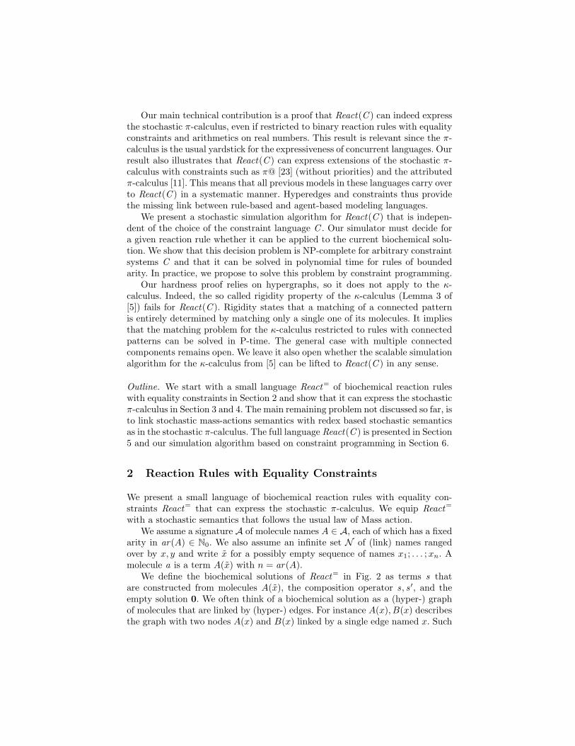
Our main technical contribution is a proof that React(C ) can indeed expressthe stochastic π-calculus, even if restricted to binary reaction rules with equalityconstraints and arithmetics on real numbers. This result is relevant since the π-calculus is the usual yardstick for the expressiveness of concurrent languages. Ourresult also illustrates that React(C ) can express extensions of the stochastic π-calculus with constraints such as π@ [23] (without priorities) and the attributedπ-calculus [11]. This means that all previous models in these languages carry overto React(C ) in a systematic manner. Hyperedges and constraints thus providethe missing link between rule-based and agent-based modeling languages.

We present a stochastic simulation algorithm for React(C ) that is indepen-dent of the choice of the constraint language C . Our simulator must decide fora given reaction rule whether it can be applied to the current biochemical solu-tion. We show that this decision problem is NP-complete for arbitrary constraintsystems C and that it can be solved in polynomial time for rules of boundedarity. In practice, we propose to solve this problem by constraint programming.

Our hardness proof relies on hypergraphs, so it does not apply to the κ-calculus. Indeed, the so called rigidity property of the κ-calculus (Lemma 3 of[5]) fails for React(C ). Rigidity states that a matching of a connected patternis entirely determined by matching only a single one of its molecules. It impliesthat the matching problem for the κ-calculus restricted to rules with connectedpatterns can be solved in P-time. The general case with multiple connectedcomponents remains open. We leave it also open whether the scalable simulationalgorithm for the κ-calculus from [5] can be lifted to React(C ) in any sense.

Outline. We start with a small language React= of biochemical reaction ruleswith equality constraints in Section 2 and show that it can express the stochasticπ-calculus in Section 3 and 4. The main remaining problem not discussed so far, isto link stochastic mass-actions semantics with redex based stochastic semanticsas in the stochastic π-calculus. The full language React(C ) is presented in Section5 and our simulation algorithm based on constraint programming in Section 6.

2 Reaction Rules with Equality Constraints

We present a small language of biochemical reaction rules with equality con-straints React= that can express the stochastic π-calculus. We equip React=

with a stochastic semantics that follows the usual law of Mass action.We assume a signature A of molecule names A ∈ A, each of which has a fixed

arity in ar(A) ∈ N0. We also assume an infinite set N of (link) names rangedover by x, y and write x for a possibly empty sequence of names x1; . . . ;xn. Amolecule a is a term A(x) with n = ar(A).

We define the biochemical solutions of React= in Fig. 2 as terms s thatare constructed from molecules A(x), the composition operator s, s ′, and theempty solution 0. We often think of a biochemical solution as a (hyper-) graphof molecules that are linked by (hyper-) edges. For instance A(x), B(x) describesthe graph with two nodes A(x) and B(x) linked by a single edge named x. Such

Solutions s ::= A(x) | s, s ′ | 0 where A ∈ A, x ∈ N

Rate expressions e ::= if x1=x2 then e1 else e2 where x1, x2 ∈ N

| e1 + e2 | e1 ∗ e2 | d and d ∈ R+0

Reaction rules r ::= se−→ (νx)s ′ where fn(r) = fn(s)

Reactions ρ ::= sd−→ s ′

Fig. 1. Syntax of reaction rules of language React=

Precongruence (s1, s2), s3 ≈ s1, (s2, s3) s1, s2 ≈ s2, s1 s,0 ≈ s

Congruences ≈ s ′ σ : N → N injective

s ≡ s ′σ

Fig. 2. Precongruence and congruence on solutions

graphs do neither depend on the order of molecules nor on the concrete choiceof link names. For instance, the same graph is obtained by solutions B(y), A(y)and A(x), B(x).

In Fig. 2, we define two congruence relations on solutions. The precongruence≈ captures order independence. It is the least equivalence relation on solutionsthat renders the composition operator “,” associative and commutative with theneutral element 0. We write [s]≈ for the equivalence class of a solution s. Clearly,we can identify precongruence classes with multisets of molecules. The weakercongruence relation ≡ accounts for the irrelevance of concrete names in addition.It is defined such that s ≡ s ′ if and only if there exists a solution s ′′ ≈ s andan injective function σ : N → N such that s ′ = s ′′σ, i.e., the term obtained byrenaming all names x in s ′′ to σ(x).

We write fn(s) for the set of names occurring in s. As usual, we define it-

erated compositions∏0

i=1 si = 0,∏n

i=1 si = (∏n−1

i=1 si), sn, and sm =∏m

i=1 s. Ifa1, . . . , an are pairwise distinct molecules then we define ·

∏n

i=1 ami

i =∏n

i=1 ami

i .Modulo precongruence, this term stands for the multiset with mi occurrences ofmolecule ai.

Reactions ρ are terms of the form s1d−→ s2. They can be applied to rewrite

solutions congruent to s, s1 to some solution congruent to s, s2:

(react)s ′1 ≡ s, s1 s, s2 ≡ s ′2

s1d−→ s2 ⊢ s ′1 → s ′2

Judgements ρ ⊢ s ′1 → s ′2 capture the non-deterministic semantics of reactions.Note that the rate constant d is irrelevant here; it matters in the stochasticsemantics only, see below.

Reaction rules r are terms of the form se−→ (νx)s ′. They are to be understood

as schemas that define sets of reactions, one reaction per substitution σ : N →

(cond1)e1 ⇓ d1

if x=x then e1 else e2 ⇓ d1(cond2)

x1 6= x2 e2 ⇓ d2

if x1=x2 then e1 else e2 ⇓ d2

(reals)d ∈ R

+0

d ⇓ d(+)

e1 ⇓ d1 e2 ⇓ d2

e1 + e2 ⇓ d1 +R d2

(∗)e1 ⇓ d1 e2 ⇓ d2

e1 ∗ e2 ⇓ d1 ∗R d2

Fig. 3. Big-step evaluator of rate expressions.

(inst)σ : fn(s) → N σ′ : {x} → N\(N ∪ fn(s)) injective eσ ⇓ d

se−→ (νx)s ′ ⇓σ,N sσ

d−→ s ′σ′σ

Fig. 4. Instantiation and evaluation of reactions rules to reactions.

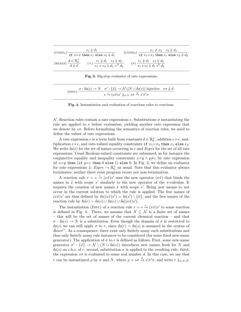
N . Reaction rules contain a rate expressions e. Substitutions σ instantiating therule are applied to e before evaluation, yielding another rate expression thatwe denote by eσ. Before formalizing the semantics of reaction rules, we need todefine the values of rate expressions.

A rate expression e is a term built from constants d ∈ R+0 , addition e+e, mul-

tiplication e ∗ e, and rate-valued equality constraints if x1=x2 then e1 else e2.We write fn(e) for the set of names occurring in e and Exprs for the set of all rateexpressions. Usual Boolean-valued constraints are subsumed, as for instance theconjunctive equality and inequality constraints x=y ∧ y 6=z by rate expressionif x=y then (if y=z then 0 else 1) else 0. In Fig. 3, we define an evaluatorfor rate expressions ⇓: Exprs → R

+0 as usual. Note that this evaluator always

terminates: neither there exist program errors nor non-termination.

A reaction rule r = se−→ (νx)s ′ uses the new operator (νx) that binds the

names in x with scope s ′ similarly to the new operator of the π-calculus. Itrequires the creation of new names x with scope s ′. Being new means to notoccur in the current solution to which the rule is applied. The free names of(νx)s ′ are thus defined by fn((νx)s ′) = fn(s ′) \ {x}, and the free names of thereaction rule by fn(r) = fn(s) ∪ fn(e) ∪ fn((νx)s ′).

The instantiation (Inst) of a reaction rule r = se−→ (νx)s ′ to some reaction

is defined in Fig. 4. There, we assume that N ⊆ N is a finite set of names– this will be the set of names of the current chemical reaction – and thatσ : fn(s) → N is a substitution. Even though the domain of σ is restricted tofn(s) we can still apply σ to r, since fn(r) = fn(s) is assumed in the syntax ofReact=. As a consequence, there exist only finitely many such substitutions andthus only finitely many rule instances to be considered (for some fixed new-namegenerator). The application of σ to r is defined as follows. First, some new-namegenerator σ′ : {x} → N \ (N ∪ fn(s)) introduces new names fresh for N andfn(s) on r.h.s. of r, second, substitution σ is applied to the resulting rule, third,the expression eσ is evaluated to some real number d. In this case, we say that

r can be instantiated ρ by σ and N , where ρ = sσd−→ s ′σ′σ, and write r ⇓σ,N ρ.

(count)s ≈ ·

∏n

i=1 amii s ′ ≈ ·

∏n+m

i=1 am′

ii

count(s; s ′) =∏n

i=1

(

m′

imi

)(reactma)

s ′1 ≈ s, s1 s, s2 ≡ s ′2

s1d−→ s2 ⊢ s ′1

d∗count(s1;s′

1)−−−−−−−−−→ s ′2

(rulesma)

s1 ≡ s ′1 d =∑

r∈R

∑

{(d′,σ) | r⇓σ,fn(s′1)ρ, ρ ⊢ s

′

1

d′−→s2}d′

R ⊢ s1d−→ma

s2

Fig. 5. Stochastic mass-action semantics of React=.

The non-deterministic semantics of a reaction rule can now be defined byreduction to the non-deterministic semantics of reactions:

(rule)r ⇓σ,fn(s) ρ ρ ⊢ s −→ s ′

r ⊢ s −→ s ′

The set of free names of the current solution s is passed over to the instantiatorr ⇓σ,fn(s) ρ, in order to ensure that new-bound names are instantiated by freshnames for the current solution. Recall that only finitely many substitutions σ :fn(r) → fn(s) are to be considered. These are the possible matchings of the lefthand side of the rule with the current solution.

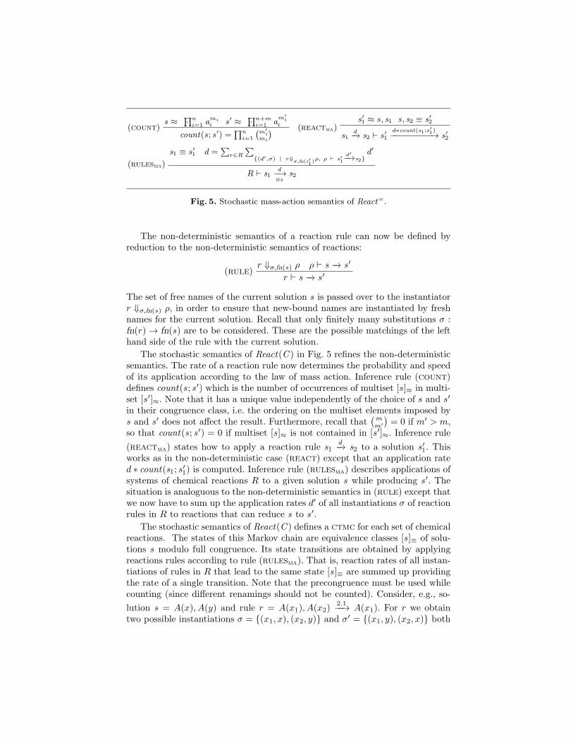
The stochastic semantics of React(C ) in Fig. 5 refines the non-deterministicsemantics. The rate of a reaction rule now determines the probability and speedof its application according to the law of mass action. Inference rule (count)defines count(s; s ′) which is the number of occurrences of multiset [s]≈ in multi-set [s ′]≈. Note that it has a unique value independently of the choice of s and s ′

in their congruence class, i.e. the ordering on the multiset elements imposed bys and s ′ does not affect the result. Furthermore, recall that

(mm′

)= 0 if m′ > m,

so that count(s; s ′) = 0 if multiset [s]≈ is not contained in [s ′]≈. Inference rule

(reactma) states how to apply a reaction rule s1d−→ s2 to a solution s ′1. This

works as in the non-deterministic case (react) except that an application rated ∗ count(s1; s

′1) is computed. Inference rule (rulesma) describes applications of

systems of chemical reactions R to a given solution s while producing s ′. Thesituation is analoguous to the non-deterministic semantics in (rule) except thatwe now have to sum up the application rates d′ of all instantiations σ of reactionrules in R to reactions that can reduce s to s ′.

The stochastic semantics of React(C ) defines a ctmc for each set of chemicalreactions. The states of this Markov chain are equivalence classes [s]≡ of solu-tions s modulo full congruence. Its state transitions are obtained by applyingreactions rules according to rule (rulesma). That is, reaction rates of all instan-tiations of rules in R that lead to the same state [s]≡ are summed up providingthe rate of a single transition. Note that the precongruence must be used whilecounting (since different renamings should not be counted). Consider, e.g., so-

lution s = A(x), A(y) and rule r = A(x1), A(x2)2.1−−→ A(x1). For r we obtain

two possible instantiations σ = {(x1, x), (x2, y)} and σ′ = {(x1, y), (x2, x)} both

(red)s1 =

∏n

i=1 ai s2 =∏n′

i=1 a′i

redex (s1; s2) = {ℓ : {1, . . . , n} → {1, . . . , n′} injective |a ′ℓ(i) = ai for all i ∈ {1, . . . , n}}

(reactred)s ′1 ≈ s, s1 s, s2 ≡ s ′2 d ∈ R

+ ℓ ∈ redex (s1; s′1)

s1d−→ s2 ⊢ s ′1

d−→ℓ

s ′2

(rulesred)

s ′1 ≡ s1 d =∑

r∈R

∑

{(d′,ℓ) | r⇓σ,fn(s′1)ρ, ρ⊢ s

′

1

d′−→ℓ

s2}d′

R ⊢ s1d

−−→red

s2

Fig. 6. Stochastic redex semantics of language React=red.

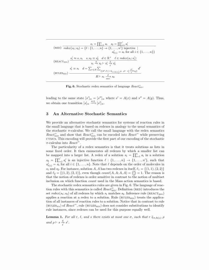
leading to the same state [s ′]≡ = [s ′′]≡ where s ′ = A(x) and s ′′ = A(y). Thus,

we obtain one transition [s]≡4.2−−→ [s ′]≡.

3 An Alternative Stochastic Semantics

We provide an alternative stochastic semantics for systems of reaction rules inthe small language that is based on redexes in analogy to the usual semantics ofthe stochastic π-calculus. We call the small language with the redex semanticsReact=red and show that React=red can be encoded into React= while preservingctmcs. This encoding will provide the first part of our encoding of the stochasticπ-calculus into React=.

The particularity of a redex semantics is that it treats solutions as lists insome fixed order. It then enumerates all redexes by which a smaller list canbe mapped into a larger list. A redex of a solution s1 =

∏n

i=1 ai in a solution

s2 =∏n′

i=1 a′i is an injective function ℓ : {1, . . . , n} → {1, . . . , n′}, such that

a ′ℓ(i) = ai for all i ∈ {1, . . . , n}. Note that ℓ depends on the order of molecules in

s1 and s2. For instance, solution A,A has two redexes in itself, ℓ1 = {(1, 1), (2, 2)}and ℓ2 = {(1, 2), (2, 1)}, even though count(A,A;A,A) =

(22

)= 1. The reason is

that the notion of redexes is order sensitive in contrast to the notion of multisetinclusion on which function count used in the Mass action semantics is based.

The stochastic redex semantics rules are given in Fig. 6. The language of reac-tion rules with this semantics is called React=red. Definition (red) introduces theset redex (s1; s2) of all redexes by which s1 matches s2. Inference rule (reactred)applies a reaction at a redex to a solution. Rule (rulesred) treats the applica-tion of all instances of reaction rules to a solution. Notice that in contrast to rule(rulesma) of React

=, rule (rulesred) does not consider substitutions to identifyrule instances, since redexes can be used for this purpose equally well.

Lemma 1. For all r, ℓ, and s there exists at most one σ, such that r ⇓σ,fn(s) ρ

and ρ ⊢ sd−→ℓ

s ′.

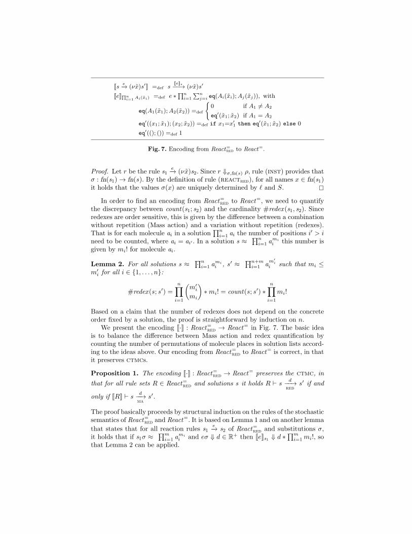
Jse−→ (νx)s ′K =def s

JeKs−−→ (νx)s ′

JeK∏ni=1 Ai(xi) =def e ∗

∏n

i=1

∑n

j=i eq(Ai(xi);Aj(xj)), with

eq(A1(x1);A2(x2)) =def

{

0 if A1 6= A2

eq′(x1; x2) if A1 = A2

eq′((x1; x1); (x2; x2)) =def if x1=x′

1 then eq′(x1; x2) else 0

eq′((); ()) =def 1

Fig. 7. Encoding from React=red to React=.

Proof. Let r be the rule s1e−→ (νx)s2. Since r ⇓σ,fn(s) ρ, rule (inst) provides that

σ : fn(s1) → fn(s). By the definition of rule (reactred), for all names x ∈ fn(s1)it holds that the values σ(x) are uniquely determined by ℓ and S. �

In order to find an encoding from React=red to React=, we need to quantifythe discrepancy between count(s1; s2) and the cardinality #redex (s1, s2). Sinceredexes are order sensitive, this is given by the difference between a combinationwithout repetition (Mass action) and a variation without repetition (redexes).That is for each molecule ai in a solution

∏n

i=1 ai the number of positions i′ > ineed to be counted, where ai = ai′ . In a solution s ≈ ·

∏n

i=1 ami

i this number isgiven by mi! for molecule ai.

Lemma 2. For all solutions s ≈ ·∏n

i=1 ami

i , s ′ ≈ ·∏n+m

i=1 am′

i

i such that mi ≤m′

i for all i ∈ {1, . . . , n}:

#redex (s; s ′) =

n∏

i=1

(m′

i

mi

)∗mi! = count(s; s ′) ∗

n∏

i=1

mi!

Based on a claim that the number of redexes does not depend on the concreteorder fixed by a solution, the proof is straightforward by induction on n.

We present the encoding J·K : React=red → React= in Fig. 7. The basic ideais to balance the difference between Mass action and redex quantification bycounting the number of permutations of molecule places in solution lists accord-ing to the ideas above. Our encoding from React=red to React= is correct, in thatit preserves ctmcs.

Proposition 1. The encoding J·K : React=red → React= preserves the ctmc, in

that for all rule sets R ∈ React=red and solutions s it holds R ⊢ sd

−−→red

s ′ if and

only if JRK ⊢ sd

−−→ma

s ′.

The proof basically proceeds by structural induction on the rules of the stochasticsemantics of React=red and React=. It is based on Lemma 1 and on another lemma

that states that for all reaction rules s1e−→ s2 of React=red and substitutions σ,

it holds that if s1σ ≈ ·∏m

i=1 ami

i and eσ ⇓ d ∈ R+ then JeKs1 ⇓ d ∗

∏m

i=1mi!, sothat Lemma 2 can be applied.

Prefixes π ::= x?y receiver where x, y, z ∈ N| x:d!z sender and d ∈ R

+0

Sums M ::= π.P prefixed process| M1 +M2 choice

Processes P,Q,O ::= A(x) defined process where A ∈ A| P1 | P2 parallel composition| (νx)P channel creation| 0 idle process

Definitions D ::= A(x) , M process definition where fn(M) ⊆ {x}

Fig. 8. Syntax of the π-calculus.

4 Expressing the Stochastic π-Calculus

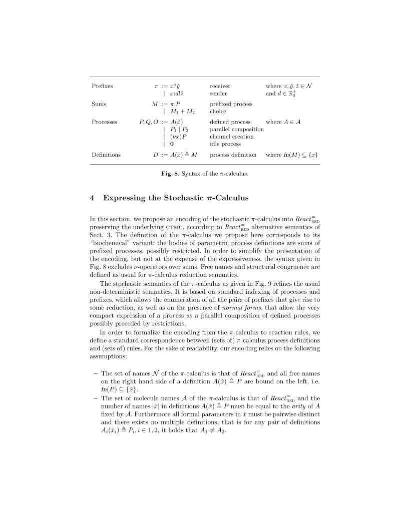
In this section, we propose an encoding of the stochastic π-calculus into React=redpreserving the underlying ctmc, according to React=red alternative semantics ofSect. 3. The definition of the π-calculus we propose here corresponds to its“biochemical” variant: the bodies of parametric process definitions are sums ofprefixed processes, possibly restricted. In order to simplify the presentation ofthe encoding, but not at the expense of the expressiveness, the syntax given inFig. 8 excludes ν-operators over sums. Free names and structural congruence aredefined as usual for π-calculus reduction semantics.

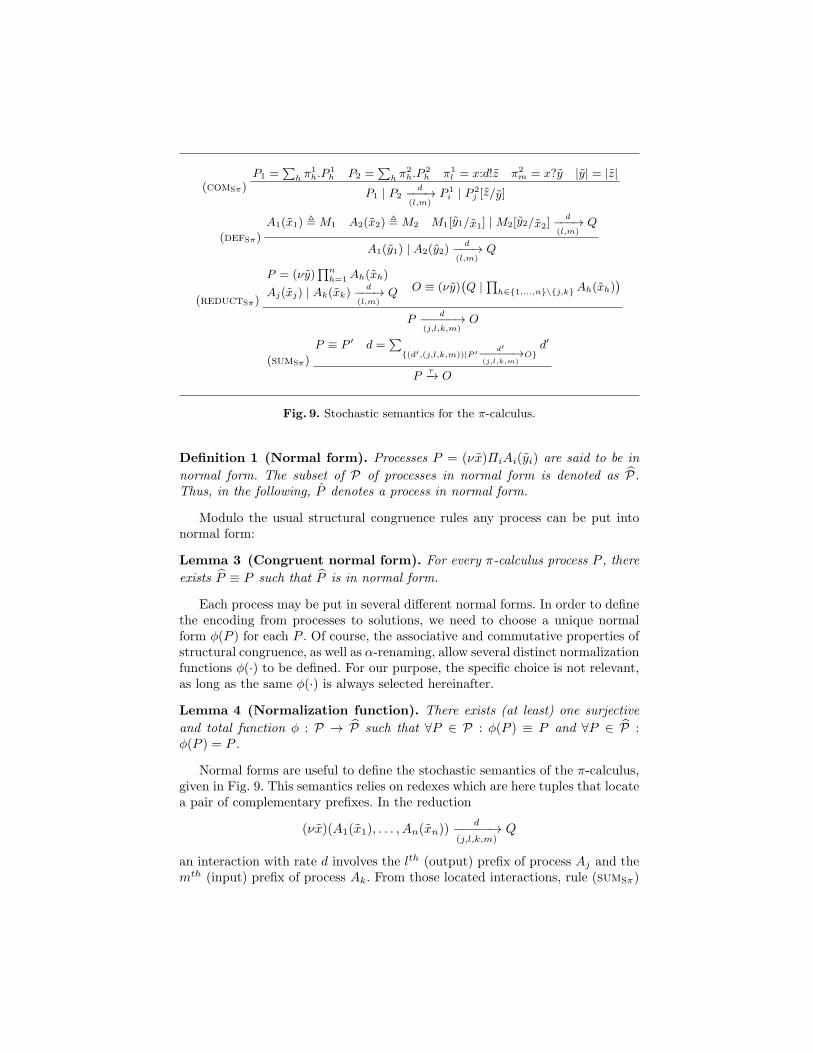
The stochastic semantics of the π-calculus as given in Fig. 9 refines the usualnon-deterministic semantics. It is based on standard indexing of processes andprefixes, which allows the enumeration of all the pairs of prefixes that give rise tosome reduction, as well as on the presence of normal forms, that allow the verycompact expression of a process as a parallel composition of defined processespossibly preceded by restrictions.

In order to formalize the encoding from the π-calculus to reaction rules, wedefine a standard correspondence between (sets of) π-calculus process definitionsand (sets of) rules. For the sake of readability, our encoding relies on the followingassumptions:

– The set of names N of the π-calculus is that of React=red and all free nameson the right hand side of a definition A(x) , P are bound on the left, i.e.fn(P ) ⊆ {x}.

– The set of molecule names A of the π-calculus is that of React=red and thenumber of names |x| in definitions A(x) , P must be equal to the arity of Afixed by A. Furthermore all formal parameters in x must be pairwise distinctand there exists no multiple definitions, that is for any pair of definitionsAi(xi) , Pi, i ∈ 1, 2, it holds that A1 6= A2.

(comSπ)P1 =

∑

h π1h.P

1h P2 =

∑

h π2h.P

2h π1

l = x:d!z π2m = x?y |y| = |z|

P1 | P2d

−−−→(l,m)

P 1i | P 2

j [z/y]

(defSπ)

A1(x1) , M1 A2(x2) , M2 M1[y1/x1] | M2[y2/x2]d

−−−→(l,m)

Q

A1(y1) | A2(y2)d

−−−→(l,m)

Q

(reductSπ)

P = (νy)∏n

h=1 Ah(xh)

Aj(xj) | Ak(xk)d

−−−→(l,m)

Q O ≡ (νy)(

Q |∏

h∈{1,...,n}\{j,k} Ah(xh))

Pd

−−−−−→(j,l,k,m)

O

(sumSπ)

P ≡ P ′ d =∑

{(d′,(j,l,k,m))|P ′d′−−−−−→

(j,l,k,m)O}

d′

Pr−→ O

Fig. 9. Stochastic semantics for the π-calculus.

Definition 1 (Normal form). Processes P = (νx)ΠiAi(yi) are said to be in

normal form. The subset of P of processes in normal form is denoted as P.Thus, in the following, P denotes a process in normal form.

Modulo the usual structural congruence rules any process can be put intonormal form:

Lemma 3 (Congruent normal form). For every π-calculus process P , there

exists P ≡ P such that P is in normal form.

Each process may be put in several different normal forms. In order to definethe encoding from processes to solutions, we need to choose a unique normalform φ(P ) for each P . Of course, the associative and commutative properties ofstructural congruence, as well as α-renaming, allow several distinct normalizationfunctions φ(·) to be defined. For our purpose, the specific choice is not relevant,as long as the same φ(·) is always selected hereinafter.

Lemma 4 (Normalization function). There exists (at least) one surjective

and total function φ : P → P such that ∀P ∈ P : φ(P ) ≡ P and ∀P ∈ P :φ(P ) = P .

Normal forms are useful to define the stochastic semantics of the π-calculus,given in Fig. 9. This semantics relies on redexes which are here tuples that locatea pair of complementary prefixes. In the reduction

(νx)(A1(x1), . . . , An(xn))d

−−−−−→(j,l,k,m)

Q

an interaction with rate d involves the lth (output) prefix of process Aj and themth (input) prefix of process Ak. From those located interactions, rule (sumSπ)

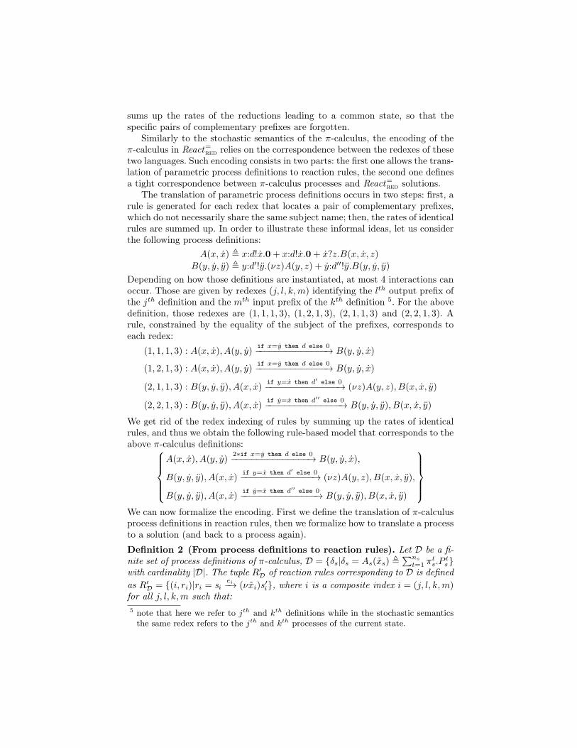
sums up the rates of the reductions leading to a common state, so that thespecific pairs of complementary prefixes are forgotten.

Similarly to the stochastic semantics of the π-calculus, the encoding of theπ-calculus in React=red relies on the correspondence between the redexes of thesetwo languages. Such encoding consists in two parts: the first one allows the trans-lation of parametric process definitions to reaction rules, the second one definesa tight correspondence between π-calculus processes and React=red solutions.

The translation of parametric process definitions occurs in two steps: first, arule is generated for each redex that locates a pair of complementary prefixes,which do not necessarily share the same subject name; then, the rates of identicalrules are summed up. In order to illustrate these informal ideas, let us considerthe following process definitions:

A(x, x) , x:d!x.0+ x:d!x.0+ x?z.B(x, x, z)

B(y, y, y) , y:d′!y.(νz)A(y, z) + y:d′′!y.B(y, y, y)

Depending on how those definitions are instantiated, at most 4 interactions canoccur. Those are given by redexes (j, l, k,m) identifying the lth output prefix ofthe jth definition and the mth input prefix of the kth definition 5. For the abovedefinition, those redexes are (1, 1, 1, 3), (1, 2, 1, 3), (2, 1, 1, 3) and (2, 2, 1, 3). Arule, constrained by the equality of the subject of the prefixes, corresponds toeach redex:

(1, 1, 1, 3) : A(x, x), A(y, y)if x=y then d else 0−−−−−−−−−−−−−−→ B(y, y, x)

(1, 2, 1, 3) : A(x, x), A(y, y)if x=y then d else 0−−−−−−−−−−−−−−→ B(y, y, x)

(2, 1, 1, 3) : B(y, y, y), A(x, x)if y=x then d′

else 0−−−−−−−−−−−−−−→ (νz)A(y, z), B(x, x, y)

(2, 2, 1, 3) : B(y, y, y), A(x, x)if y=x then d′′

else 0−−−−−−−−−−−−−−−→ B(y, y, y), B(x, x, y)

We get rid of the redex indexing of rules by summing up the rates of identicalrules, and thus we obtain the following rule-based model that corresponds to theabove π-calculus definitions:

A(x, x), A(y, y)2∗if x=y then d else 0−−−−−−−−−−−−−−−→ B(y, y, x),

B(y, y, y), A(x, x)if y=x then d′

else 0−−−−−−−−−−−−−−→ (νz)A(y, z), B(x, x, y),

B(y, y, y), A(x, x)if y=x then d′′

else 0−−−−−−−−−−−−−−−→ B(y, y, y), B(x, x, y)

We can now formalize the encoding. First we define the translation of π-calculusprocess definitions in reaction rules, then we formalize how to translate a processto a solution (and back to a process again).

Definition 2 (From process definitions to reaction rules). Let D be a fi-nite set of process definitions of π-calculus, D = {δs|δs = As(xs) ,

∑ns

t=1 πts.P

ts}

with cardinality |D|. The tuple R′D of reaction rules corresponding to D is defined

as R′D = {(i, ri)|ri = si

ei−→ (νxi)s′i}, where i is a composite index i = (j, l, k,m)

for all j, l, k,m such that:

5 note that here we refer to jth and kth definitions while in the stochastic semanticsthe same redex refers to the jth and kth processes of the current state.

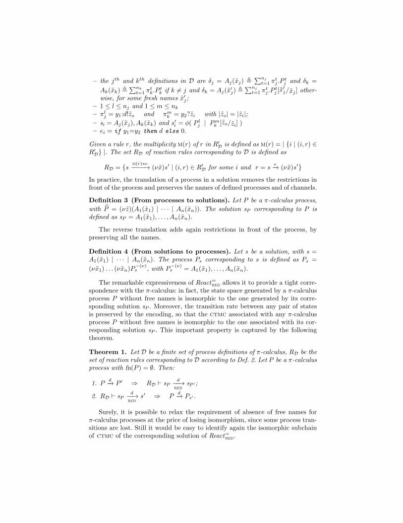
– the jth and kth definitions in D are δj = Aj(xj) ,∑nj

t=1 πtj .P

tj and δk =

Ak(xk) ,∑nk

t=1 πtk.P

tk if k 6= j and δk = Aj(x

′j) ,

∑nj

t=1 πtj .P

tj [x

′j/xj ] other-

wise, for some fresh names x′j;– 1 ≤ l ≤ nj and 1 ≤ m ≤ nk– πl

j = y1:d!zo and πmk = y2?zi with |zo| = |zi|;

– si = Aj(xj), Ak(xk) and s ′i = φ( P lj | Pm

k [zo/zi] )– ei = if y1=y2 then d else 0.

Given a rule r, the multiplicity m(r) of r in R′D is defined as m(r) = | {i | (i, r) ∈

R′D} |. The set RD of reaction rules corresponding to D is defined as

RD = {sm(r)∗e−−−−→ (νx)s ′ | (i, r) ∈ R′

D for some i and r = se−→ (νx)s ′}

In practice, the translation of a process in a solution removes the restrictions infront of the process and preserves the names of defined processes and of channels.

Definition 3 (From processes to solutions). Let P be a π-calculus process,

with P = (νz)(A1(x1) | · · · | An(xn)). The solution sP corresponding to P isdefined as sP = A1(x1), . . . , An(xn).

The reverse translation adds again restrictions in front of the process, bypreserving all the names.

Definition 4 (From solutions to processes). Let s be a solution, with s =A1(x1) | · · · | An(xn). The process Ps corresponding to s is defined as Ps =

(νx1) . . . (νxn)P−(ν)s , with P

−(ν)s = A1(x1), . . . , An(xn).

The remarkable expressiveness of React=red allows it to provide a tight corre-spondence with the π-calculus: in fact, the state space generated by a π-calculusprocess P without free names is isomorphic to the one generated by its corre-sponding solution sP . Moreover, the transition rate between any pair of statesis preserved by the encoding, so that the ctmc associated with any π-calculusprocess P without free names is isomorphic to the one associated with its cor-responding solution sP . This important property is captured by the followingtheorem.

Theorem 1. Let D be a finite set of process definitions of π-calculus, RD be theset of reaction rules corresponding to D according to Def. 2. Let P be a π-calculusprocess with fn(P ) = ∅. Then:

1. Pd−→ P ′ ⇒ RD ⊢ sP

d−−→red

sP ′ ;

2. RD ⊢ sPd

−−→red

s ′ ⇒ Pd−→ Ps′ .

Surely, it is possible to relax the requirement of absence of free names forπ-calculus processes at the price of losing isomorphism, since some process tran-sitions are lost. Still it would be easy to identify again the isomorphic subchainof ctmc of the corresponding solution of React=red.

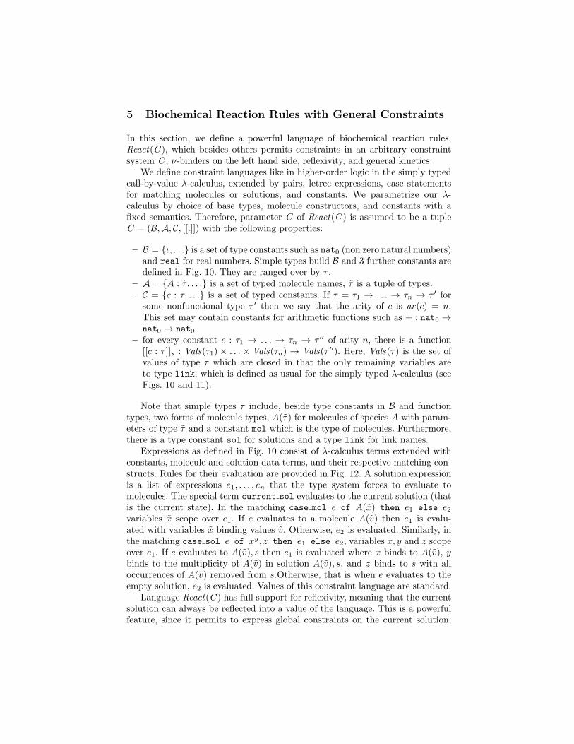
5 Biochemical Reaction Rules with General Constraints

In this section, we define a powerful language of biochemical reaction rules,React(C ), which besides others permits constraints in an arbitrary constraintsystem C , ν-binders on the left hand side, reflexivity, and general kinetics.

We define constraint languages like in higher-order logic in the simply typedcall-by-value λ-calculus, extended by pairs, letrec expressions, case statementsfor matching molecules or solutions, and constants. We parametrize our λ-calculus by choice of base types, molecule constructors, and constants with afixed semantics. Therefore, parameter C of React(C ) is assumed to be a tupleC = (B,A, C, [[.]]) with the following properties:

– B = {ι, . . .} is a set of type constants such as nat0 (non zero natural numbers)and real for real numbers. Simple types build B and 3 further constants aredefined in Fig. 10. They are ranged over by τ .

– A = {A : τ , . . .} is a set of typed molecule names, τ is a tuple of types.– C = {c : τ, . . .} is a set of typed constants. If τ = τ1 → . . . → τn → τ ′ for

some nonfunctional type τ ′ then we say that the arity of c is ar(c) = n.This set may contain constants for arithmetic functions such as + : nat0 →nat0 → nat0.

– for every constant c : τ1 → . . . → τn → τ ′′ of arity n, there is a function[[c : τ ]]s : Vals(τ1) × . . . × Vals(τn) → Vals(τ ′′). Here, Vals(τ) is the set ofvalues of type τ which are closed in that the only remaining variables areto type link, which is defined as usual for the simply typed λ-calculus (seeFigs. 10 and 11).

Note that simple types τ include, beside type constants in B and functiontypes, two forms of molecule types, A(τ) for molecules of species A with param-eters of type τ and a constant mol which is the type of molecules. Furthermore,there is a type constant sol for solutions and a type link for link names.

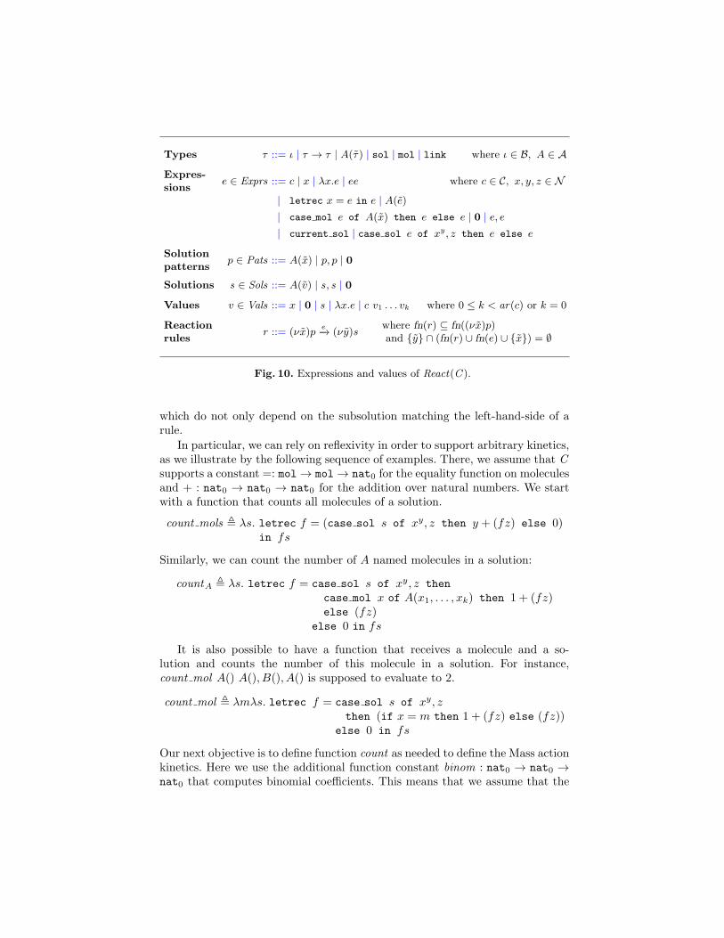
Expressions as defined in Fig. 10 consist of λ-calculus terms extended withconstants, molecule and solution data terms, and their respective matching con-structs. Rules for their evaluation are provided in Fig. 12. A solution expressionis a list of expressions e1, . . . , en that the type system forces to evaluate tomolecules. The special term current sol evaluates to the current solution (thatis the current state). In the matching case mol e of A(x) then e1 else e2variables x scope over e1. If e evaluates to a molecule A(v) then e1 is evalu-ated with variables x binding values v. Otherwise, e2 is evaluated. Similarly, inthe matching case sol e of xy, z then e1 else e2, variables x, y and z scopeover e1. If e evaluates to A(v), s then e1 is evaluated where x binds to A(v), ybinds to the multiplicity of A(v) in solution A(v), s, and z binds to s with alloccurrences of A(v) removed from s.Otherwise, that is when e evaluates to theempty solution, e2 is evaluated. Values of this constraint language are standard.

Language React(C ) has full support for reflexivity, meaning that the currentsolution can always be reflected into a value of the language. This is a powerfulfeature, since it permits to express global constraints on the current solution,

Types τ ::= ι | τ → τ | A(τ) | sol | mol | link where ι ∈ B, A ∈ A

Expres-

sionse ∈ Exprs ::= c | x | λx.e | ee where c ∈ C, x, y, z ∈ N

| letrec x = e in e | A(e)

| case mol e of A(x) then e else e | 0 | e, e

| current sol | case sol e of xy, z then e else e

Solution

patternsp ∈ Pats ::= A(x) | p, p | 0

Solutions s ∈ Sols ::= A(v) | s, s | 0

Values v ∈ Vals ::= x | 0 | s | λx.e | c v1 . . . vk where 0 ≤ k < ar(c) or k = 0

Reaction

rulesr ::= (νx)p

e−→ (νy)s

where fn(r) ⊆ fn((νx)p)and {y} ∩ (fn(r) ∪ fn(e) ∪ {x}) = ∅

Fig. 10. Expressions and values of React(C ).

which do not only depend on the subsolution matching the left-hand-side of arule.

In particular, we can rely on reflexivity in order to support arbitrary kinetics,as we illustrate by the following sequence of examples. There, we assume that Csupports a constant =: mol → mol → nat0 for the equality function on moleculesand + : nat0 → nat0 → nat0 for the addition over natural numbers. We startwith a function that counts all molecules of a solution.

count mols , λs. letrec f = (case sol s of xy, z then y + (fz) else 0)in fs

Similarly, we can count the number of A named molecules in a solution:

countA , λs. letrec f = case sol s of xy, z then

case mol x of A(x1, . . . , xk) then 1 + (fz)else (fz)

else 0 in fs

It is also possible to have a function that receives a molecule and a so-lution and counts the number of this molecule in a solution. For instance,count mol A() A(), B(), A() is supposed to evaluate to 2.

count mol , λmλs. letrec f = case sol s of xy, zthen (if x = m then 1 + (fz) else (fz))

else 0 in fs

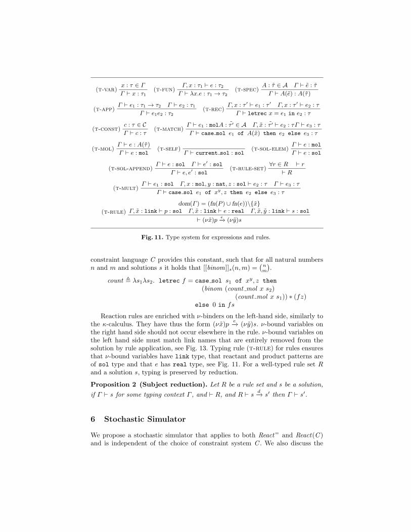
Our next objective is to define function count as needed to define the Mass actionkinetics. Here we use the additional function constant binom : nat0 → nat0 →nat0 that computes binomial coefficients. This means that we assume that the

(t-var)x : τ ∈ Γ

Γ ⊢ x : τ1(t-fun)

Γ, x : τ1 ⊢ e : τ2

Γ ⊢ λx.e : τ1 → τ2(t-spec)

A : τ ∈ A Γ ⊢ e : τ

Γ ⊢ A(e) : A(τ)

(t-app)Γ ⊢ e1 : τ1 → τ2 Γ ⊢ e2 : τ1

Γ ⊢ e1e2 : τ2(t-rec)

Γ, x : τ ′ ⊢ e1 : τ ′ Γ, x : τ ′ ⊢ e2 : τ

Γ ⊢ letrec x = e1 in e2 : τ

(t-const)c : τ ∈ C

Γ ⊢ c : τ(t-match)

Γ ⊢ e1 : molA : τ ′ ∈ A Γ, x : τ ′ ⊢ e2 : τΓ ⊢ e3 : τ

Γ ⊢ case mol e1 of A(x) then e2 else e3 : τ

(t-mol)Γ ⊢ e : A(τ)

Γ ⊢ e : mol(t-self)

Γ ⊢ current sol : sol(t-sol-elem)

Γ ⊢ e : mol

Γ ⊢ e : sol

(t-sol-append)Γ ⊢ e : sol Γ ⊢ e′ : sol

Γ ⊢ e, e′ : sol(t-rule-set)

∀r ∈ R ⊢ r

⊢ R

(t-mult)Γ ⊢ e1 : sol Γ, x : mol, y : nat, z : sol ⊢ e2 : τ Γ ⊢ e3 : τ

Γ ⊢ case sol e1 of xy, z then e2 else e3 : τ

(t-rule)

dom(Γ ) = (fn(P ) ∪ fn(e))\{x}Γ, x : link ⊢ p : sol Γ, x : link ⊢ e : real Γ, x, y : link ⊢ s : sol

⊢ (νx)pe−→ (νy)s

Fig. 11. Type system for expressions and rules.

constraint language C provides this constant, such that for all natural numbersn and m and solutions s it holds that [[binom]]s(n,m) =

(nm

).

count , λs1λs2. letrec f = case sol s1 of xy, z then

(binom (count mol x s2)(count mol x s1)) ∗ (fz)

else 0 in fs

Reaction rules are enriched with ν-binders on the left-hand side, similarly tothe κ-calculus. They have thus the form (νx)p

e−→ (νy)s. ν-bound variables on

the right hand side should not occur elsewhere in the rule. ν-bound variables onthe left hand side must match link names that are entirely removed from thesolution by rule application, see Fig. 13. Typing rule (t-rule) for rules ensuresthat ν-bound variables have link type, that reactant and product patterns areof sol type and that e has real type, see Fig. 11. For a well-typed rule set Rand a solution s, typing is preserved by reduction.

Proposition 2 (Subject reduction). Let R be a rule set and s be a solution,

if Γ ⊢ s for some typing context Γ , and ⊢ R, and R ⊢ sd−→ s ′ then Γ ⊢ s ′.

6 Stochastic Simulator

We propose a stochastic simulator that applies to both React= and React(C )and is independent of the choice of constraint system C . We also discuss the

v ⇓s v

e1 ⇓s λx.e e2 ⇓s v′ e[v′/x] ⇓s v

e1e2 ⇓s v

e1 ⇓s v1 6= λx.e e2 ⇓s v2 v1v2 ⇓s v

e1e2 ⇓s v

c : τ ∈ C ar(x) = n e1 ⇓s v1 . . . en ⇓s vn

c e1 . . . en ⇓s [[c]]s(v1, . . . , vn)

e2[e1/x] ⇓s v

letrec x = e1 in e2 ⇓s v

e ⇓s v

A(e) ⇓s A(v)

e1 ⇓s A(v′) e2[v′/x] ⇓s v

case mol e1 of A(x) then e2 else e3 ⇓s v

e1 ⇓s B(v′) A 6= B e3 ⇓s v

case mol e1 of A(x) then e2 else e3 ⇓s v

e1 ⇓s s1 s1 ≡ ·∏n

i=1 amii s1 = a1, s

′1 s2 ≡ ·

∏n

i=2 amii e2[a/x,m1/y, s2/z] ⇓s v

case sol e1 of xy, z then e2 else e3 ⇓s v

e1 ⇓s 0 e3 ⇓s v

case sol e1 of xy, z then e2 else e3 ⇓s v

e ⇓s s e′ ⇓s s ′

e, e′ ⇓s s, s ′ current sol ⇓s s

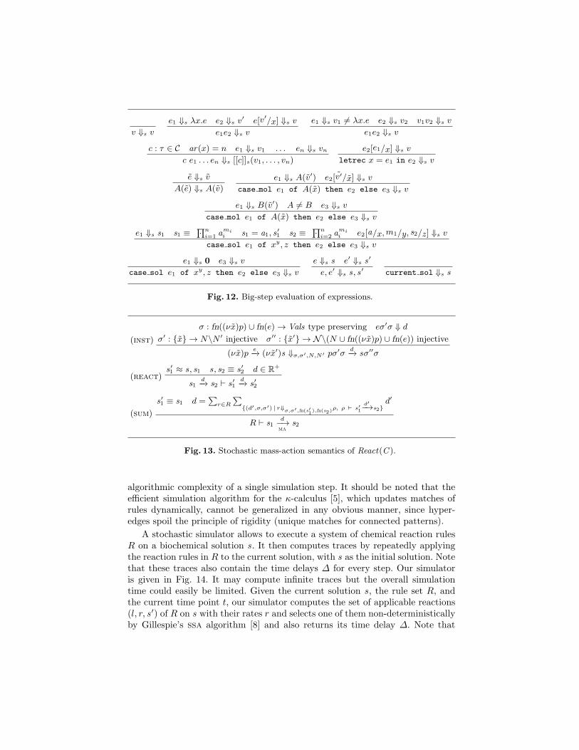
Fig. 12. Big-step evaluation of expressions.

(inst)

σ : fn((νx)p) ∪ fn(e) → Vals type preserving eσ′σ ⇓ d

σ′ : {x} → N\N ′ injective σ′′ : {x′} → N\(N ∪ fn((νx)p) ∪ fn(e)) injective

(νx)pe−→ (νx′)s ⇓σ,σ′,N,N′ pσ′σ

d−→ sσ′′σ

(react)s ′1 ≈ s, s1 s, s2 ≡ s ′2 d ∈ R

+

s1d−→ s2 ⊢ s ′1

d−→ s ′2

(sum)

s ′1 ≡ s1 d =∑

r∈R

∑

{(d′,σ,σ′) | r⇓σ,σ′,fn(s′1),fn(s2)ρ, ρ ⊢ s

′

1

d′−→s2}d′

R ⊢ s1d−→ma

s2

Fig. 13. Stochastic mass-action semantics of React(C ).

algorithmic complexity of a single simulation step. It should be noted that theefficient simulation algorithm for the κ-calculus [5], which updates matches ofrules dynamically, cannot be generalized in any obvious manner, since hyper-edges spoil the principle of rigidity (unique matches for connected patterns).

A stochastic simulator allows to execute a system of chemical reaction rulesR on a biochemical solution s. It then computes traces by repeatedly applyingthe reaction rules in R to the current solution, with s as the initial solution. Notethat these traces also contain the time delays ∆ for every step. Our simulatoris given in Fig. 14. It may compute infinite traces but the overall simulationtime could easily be limited. Given the current solution s, the rule set R, andthe current time point t, our simulator computes the set of applicable reactions(l, r, s ′) of R on s with their rates r and selects one of them non-deterministicallyby Gillespie’s ssa algorithm [8] and also returns its time delay ∆. Note that

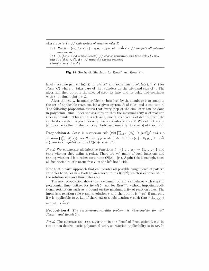
s imulate (s, t) // with system of reaction rules R

l et Reacts = {(d, (l, r, s ′)) | r ∈ R, r ⇓l ρ, ρ ⊢ sd−→ s ′} // compute all potential

reaction stepsl et (d, (l, r, s ′), ∆) = ssa(Reacts) // choose transition and time delay by ssaoutput (d, (l, r, s ′), ∆) // trace the chosen reactions imulate (s ′, t+∆)

Fig. 14. Stochastic Simulator for React= and React(C ).

label l is some pair (σ, fn(s ′)) for React= and some pair (σ, σ′, fn(s), fn(s ′)) forReact(C ) where σ′ takes care of the ν-binders on the left-hand side of r. Thealgorithm then outputs the selected step, its rate, and its delay and continueswith s ′ at time point t+∆.

Algorithmically, the main problem to be solved by the simulator is to computethe set of applicable reactions for a given system R of rules and a solution s.The following proposition states that every step of the simulator can be donein polynomial time under the assumption that the maximal arity n of reactionrules is bounded. This result is relevant, since the encoding of definitions of thestochastic π-calculus produces only reactions rules of arity 2. We define the size|r| of a rule as the number of its symbols, and similarly the size |s| of a solution.

Proposition 3. Let r be a reaction rule (νx)∏n

i=1Ai(xi)e−→ (νx′)p′ and s a

solution∏m

j=1A′j(v

′j) then the set of possible instantiations {l | r ⇓l ρ, ρ ⊢ s

d−→

s ′} can be computed in time O(|r|+ |s|+mn).

Proof. We enumerate all injective functions ℓ : {1, . . . , n} → {1, . . . ,m} andtests whether they define a redex. There are mn many of such functions andtesting whether ℓ is a redex costs time O(|s| + |r|). Again this is enough, sinceall free variables of r occur freely on the left hand side. �

Note that a naive approach that enumerates all possible assignments of patternvariables to values in s leads to an algorithm in O(|r||s|) which is exponential inthe solution size and thus unfeasible.

The next proposition shows that we cannot obtain a simulator with steps inpolynomial time, neither for React(C ) nor for React=, without imposing addi-tional restrictions such as a bound on the maximal arity of reaction rules. Theinput is a reaction rule r and a solution s and the output is “yes” if and onlyif r is applicable to s, i.e., if there exists a substitution σ such that r ⇓σ,fn(s) ρ

and ρ ⊢ sd−→ s ′.

Proposition 4. The reaction-applicability problem is np-complete for bothReact= and React(C ).

Proof. The generate and test algorithm in the Proof of Proposition 3 can berun in non-deterministic polynomial time, so reaction applicability is in np. In

order to prove np-hardness, we show that 3SAT can be reduced to reaction-applicability in polynomial time. We illustrate the ideas of our encoding at thefollowing two 3SAT clauses as an example.

(b1 ∨ b2) ∧ (b1 ∨ b2 ∨ b3)

We now express theses clauses by a reaction rule pd−→ s ′ that is supposed to

match a solution s. For each of the two clauses Ci where 1 ≤ i ≤ 2, we fixa variable xi which will match either of the three Boolean variable b1, b2, b3and that zi matches the value of this Boolean variable in variable assignmentssatisfying the clauses. We use molecule names in A = {Ci, Eij | 1 ≤ i, j ≤ 2}.

1. The first clause is expressed by adding a reactant C1(x1, z1) to pattern pand molecules C1(b1, 1), C1(b2, 0) to the solution s.

2. The second clause is expressed by adding a reactant C2(x2, z2) to pattern pand molecules C2(b1, 1), C2(b2, 1), C2(b3, 0) to the solution s.

3. In order to express that zi must match the Boolean that is assigned to theBoolean variable matching xi, we encode condition xi = xj ⇒ zi = zj for all1 ≤ i < j ≤ 2. This can be done by adding the reactants Eij(xi, xj , zi, zj)to pattern p and the following molecules to solution s:∏

β,β′∈B

∏1≤k 6=l≤3Eij(bk, bk, β, β), Eij(bk, bl, β, β

′)

So if xi and xj match the same bk then zi and zj must match the sameBoolean β. Otherwise, there is no restriction.

Pattern p grows linearly in the size of the clauses, while solution s grows both,quadratically with the number of clauses and quadratically with the number ofBoolean variables, and thus polynomially in the size of the clauses. �

Computing matching redexes by constraint programming. We propose to useconstraint programming in order to find an algorithm that computes the set ofapplicable reactions for a given system R of reaction rules and a biochemicalsolution s with a complexity less than the worst complexity O(|r| + |s| +mn).This is relevant, since this algorithm will always need quadratic time for eachstep of binary rules, while one would hope for linear time in many cases.

Rather than generating all redex candidates ℓ and then testing whether ℓ isindeed a redex of r and s, we define a constraint that states whether a redexcandidate for a solution is indeed a redex and then solve this constraint byconstraint programming, i.e. by propagating and splitting rather than generatingand testing. For a given solution s = ·

∏n

i=1 ami

i and a reaction∏m

i=1 pie−→ s ′,

the constraint ψ(r, s) is defined as follows:

ψ(∏m

i=1 pie−→ s ′, ·

∏n

i=1 ami

i ) = e ⇓ d ∈ R+ ∧m

i=1Ii ∈ {1, . . . , n} ∧ pi = aIi∧∧mi=1#{j | Ii = Ij} ≤ mi

We use finite domain variables Ii and so called element constraints for express-ing ∧m

i=1Ii ∈ {1, . . . , n} ∧ pi = aIi which states that all pi match aIi (line 2).Strong propagators for element constraints are provided by all current constraintprogramming libraries. Additional requirements are that the number of patternsmatched to the same molecule must not exceed the number of that molecule inthe solution (line 3) and that e evaluates to a successful value (line 1).

7 Conclusion

We introduced a new language of biochemical reaction rules with constraintsReact(C ) that is highly expressive. We sowed that with equality constraints andhyperedges the missing features for subsuming the expressiveness of the stochas-tic π-calculus are provided. Besides constraints React(C ) supports reflexivity,which enables modelers to define arbitrary kinetics.

We presented a simulator for React(C ) that computes steps in polynomialtime, under the assumption that the arity of reaction rules is bounded. Weshowed that efficient simulation is impossible without this assumption. A con-straint programming solution that may often avoid the higher polynomials inthe worst case was presented. An implementation is under way.

In future work, we would like to show that the attributed π-calculus π(C )can be encoded in React(C ) restricted to binary rules. Furthermore, we conjec-ture that the imperative π-calculus can be encoded into React(C ) restricted toternary rules. This would prove that React(C ) subsumes BioAmbients as well.The relationship of React(C ) to Bigraphs is also to be elaborated.

References

1. ML. Blinov, JR. Faeder, B. Goldstein, and WS. Hlavacek. Bionetgen: software forrule-based modeling of signal transduction based on the interactions of moleculardomains. Bioinformatics, 20(17):3289–3291, 2004.

2. L. Cardelli. From processes to odes by chemistry. In IFIP TCS, volume 273 ofIFIP, pages 261–281. 2008.

3. N. Chabrier-Rivier, F. Fages, and S. Soliman. The biochemical abstract machinebiocham. In Computational Methods in Systems Biology, International ConferenceCMSB 2004, volume 3082 of LNCS, pages 172–191. 2005.

4. V. Danos, J. Feret, W. Fontana, R. Harmer, and J. Krivine. Abstracting thedifferential semantics of rule-based models: Exact and automated model reduction.In 25th LICS, pages 362–381. IEEE Press, 2010.

5. V. Danos, J. Feret, W. Fontana, and J. Krivine. Scalable simulation of cellular sig-naling networks. In Programming Languages and Systems, 5th Asian Symposium,volume 4807 of LNCS, pages 139–157. 2007.

6. V. Danos and C. Laneve. Formal molecular biology. TCS, 325(1):69–110, 2004.7. C. Fournet and G. Gonthier. The reflexive cham and the join-calculus. In POPL,

pages 372–385, ACM press, 1996.8. DT. Gillespie. A general method for numerically simulating the stochastic time evo-

lution of coupled chemical reactions. Journal of Computational Physics, 22(4):403– 434, 1976.

9. SW. Gilroy and MD. Harrison. SBML: a user interface mark-up language basedon interaction style. Int. J. Web Eng. Technol., 4(2):207–234, 2008.

10. M. John, C. Lhoussaine, and J. Niehren. Dynamic compartments in the impera-tive pi calculus. In Computational Methods in Systems Biology, 7th InternationalConference, volume 5688 of LNCS, pages 235–250. 2009.

11. M. John, C. Lhoussaine, J. Niehren, and A. Uhrmacher. The attributed pi calculuswith priorities. Trans. on Computational Systems Biology, 5945(XII):13–76, 2010.

12. J. Krivine, V. Danos, and A. Benecke. Modelling epigenetic information mainte-nance: A kappa tutorial. In 21st CAV, volume 5643 of LNCS, pages 17–32. 2009.

13. C. Kuttler, C. Lhoussaine, and M. Nebut. Rule-based modeling of transcriptionalattenuation at the tryptophan operon. Trans. on Computational Systems Biology,5945(XII):199–228, 2010.

14. C. Kuttler, C. Lhoussaine, and J. Niehren. A stochastic pi calculus for concurrentobjects. In Second International Conference on Algebraic Biology, volume 4545 ofLNCS, pages 232–246. 2007.

15. C. Laneve, S. Pradalier, and G. Zavattaro. From biochemistry to stochastic pro-cesses. ENTCS, 253(3):167–185, 2009.

16. N. Papanikolaou. The space and motion of communicating agents author: RobinMilner SIGACT News, 41(3):51–55, 2010.

17. A. Phillips and L. Cardelli. Efficient, correct simulation of biological processes inthe stochastic pi-calculus. In Computational Methods in Systems Biology, Inter-national Conference, volume 4695 of LNCS, pages 184–199. 2007.

18. C. Priami. Stochastic pi-calculus. Comput. J., 38(7):578–589, 1995.19. S. Ramsey, D. Orrell, and H. Bolouri. Dizzy: Stochastic simulation of large-scale ge-

netic regulatory networks. J. Bioinformatics and Computational Biology, 3(2):415–436, 2005.

20. A. Regev, E. M. Panina, W. Silverman, L. Cardelli, and E. Y. Shapiro. Bioambi-ents: an abstraction for biological compartments. TCS, 325(1):141–167, 2004.

21. A. Regev and E. Shapiro. Cells as Computation. Nature, 419:343, 2002.22. A. Romanel and C. Priami. On the computational power of BlenX. TCS,

411(2):542–565, 2010.23. C. Versari. A core calculus for a comparative analysis of bio-inspired calculi. In

ESOP, volume 4421 of LNCS, pages 411–425. 2007.