BIO5312 BiostatisticsBIO5312 Biostatistics Lecture 04: Central Limit Theorem and Three Lecture 04: Central Limit Theorem and Three

Distributions Derived from the Normal Distributions Derived from the Normal Distribution Distribution

Dr. Junchao Xia

Center of Biophysics and Computational Biology

Fall 2016

9/21/2016 1/23

In this lecture we will talk about main concepts as listed below,

Expected value and variance of functions of random variables

Linear combination of random variables

Moments and moment generating function

Theoretical derivation of the central limit theorem

Three distributions derived from the normal distribution

IntroductionIntroduction

9/21/2016 2/23

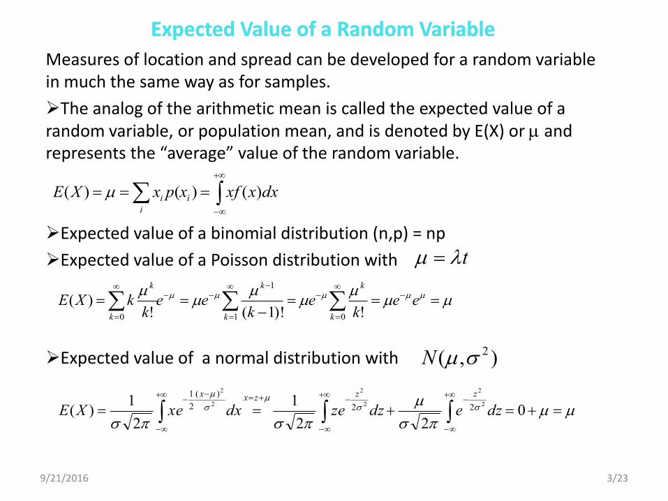
Measures of location and spread can be developed for a random variable in much the same way as for samples.

The analog of the arithmetic mean is called the expected value of a random variable, or population mean, and is denoted by E(X) or and represents the “average” value of the random variable.

Expected value of a binomial distribution (n,p) = np

Expected value of a Poisson distribution with

Expected value of a normal distribution with

Expected Value of a Random VariableExpected Value of a Random Variable

9/21/2016

dxxxfxpxXE i

i

i )()()(

eek

ek

eek

kXEk

k

k

k

k

k

01

1

0 !)!1(!)(

t

),( 2N

022

1

2

1)(

2

2

2

2

2

2

22

)(

2

1

dzedzzedxxeXE

zzzxx

3/23

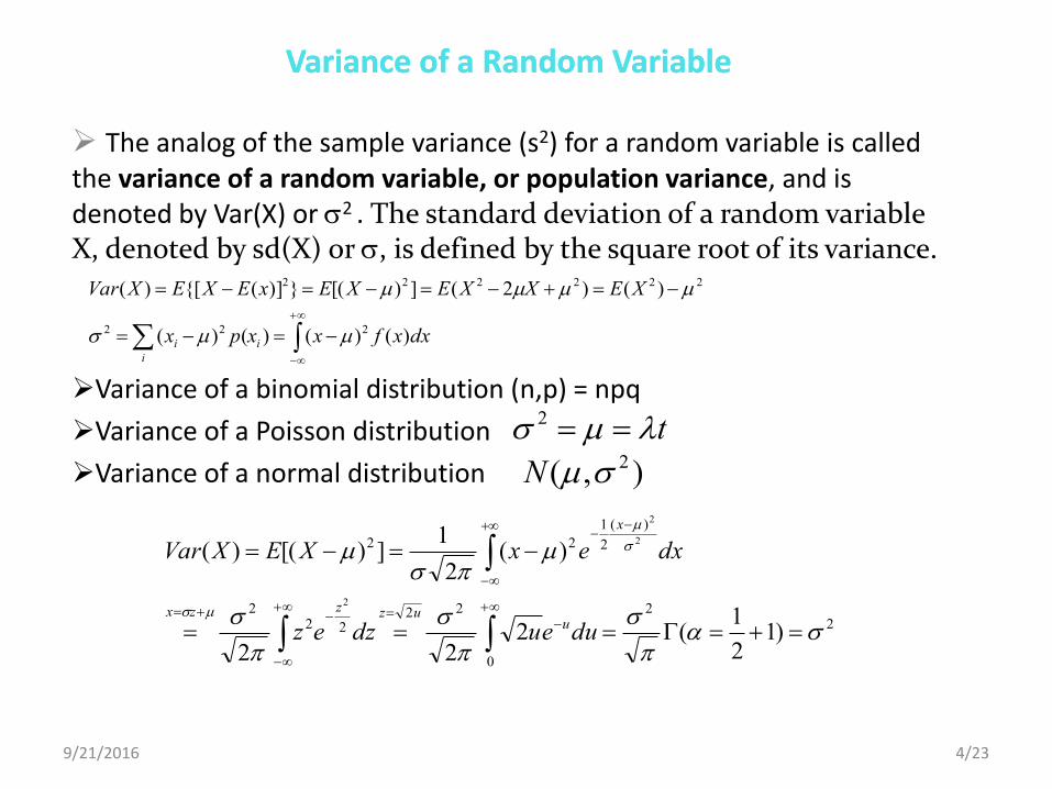
The analog of the sample variance (s2) for a random variable is called the variance of a random variable, or population variance, and is denoted by Var(X) or 2 . The standard deviation of a random variable X, denoted by sd(X) or , is defined by the square root of its variance.

Variance of a binomial distribution (n,p) = npq

Variance of a Poisson distribution

Variance of a normal distribution

Variance of a Random VariableVariance of a Random Variable

9/21/2016

dxxfxxpx

XEXXEXExEXEXVar

i

i

i )()()()(

)()2(])[(})]({[)(

222

222222

t 2

),( 2N

22

0

2222

2

)(

2

1

22

)12

1(2

22

)(2

1])[()(

2

2

2

dueudzez

dxexXEXVar

uuzzzx

x

4/23

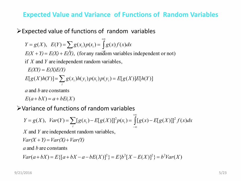
Expected value of functions of random variables

Variance of functions of random variables

Expected Value and Variance of Functions of Random VariablesExpected Value and Variance of Functions of Random Variables

9/21/2016

dxxfxgxpxgYEXgY i

i

i )()()()()( ),(

)()(

constants are and

)]([)]([)()()()()]()([

, variablesrandomt independen are and if

not)or t independen variablesrandomany (for ,

XbEabXaE

ba

YhEXgEypxpyhxgYhXgE

E(X)E(Y)E(XY)

YX

E(Y)E(X)Y)E(X

ii

i

ii

dxxfXgExgxpXgExgYVarXgY i

i

i )()]]([)([)()]]([)([)( ),( 22

)(})]([{})]({[)(

constants are and

, variablesrandomt independen are and

2222 XVarbXEXbEXbEabXaEbXaVar

ba

Var(Y)Var(X)Y)Var(X

YX

5/23

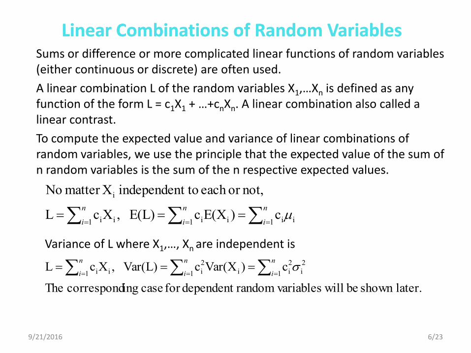
Sums or difference or more complicated linear functions of random variables (either continuous or discrete) are often used.

A linear combination L of the random variables X1,…Xn is defined as any function of the form L = c1X1 + …+cnXn. A linear combination also called a linear contrast.

To compute the expected value and variance of linear combinations of random variables, we use the principle that the expected value of the sum of n random variables is the sum of the n respective expected values.

Variance of L where X1,…, Xn are independent is

n

i

n

i

n

i 1 ii1 ii1 ii

i

c)E(XcE(L) ,XcL

not,or each t toindependen Xmatter No

later.shown be will variablesrandomdependent for case ingcorrespond The

c)Var(XcVar(L) ,XcL 2

i1

2

i1 i

2

i1 ii

n

i

n

i

n

i

Linear Combinations of Random VariablesLinear Combinations of Random Variables

9/21/2016 6/23

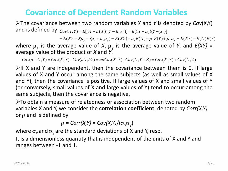
The covariance between two random variables X and Y is denoted by Cov(X,Y) and is defined by

where x is the average value of X, y is the average value of Y, and E(XY) = average value of the product of X and Y.

If X and Y are independent, then the covariance between them is 0. If large values of X and Y occur among the same subjects (as well as small values of X and Y), then the covariance is positive. If large values of X and small values of Y (or conversely, small values of X and large values of Y) tend to occur among the same subjects, then the covariance is negative.

To obtain a measure of relatedness or association between two random variables X and Y, we consider the correlation coefficient, denoted by Corr(X,Y) or and is defined by

= Corr(X,Y) = Cov(X,Y)/(xy)

where x and y are the standard deviations of X and Y, resp.

It is a dimensionless quantity that is independent of the units of X and Y and ranges between -1 and 1.

Covariance of Dependent Random VariablesCovariance of Dependent Random Variables

9/21/2016

)()()()()()()(

)])([())]())(([(),(

YEXEXYEYEXEXYEYXXYE

YXEYEYXEXEYXCov

yxxyyxxy

yx

),(),(),( ),,(),( ),,(),( ZXCovYXCovZYXCovYXabCovbYaXCovYXCovYXaCov

7/23

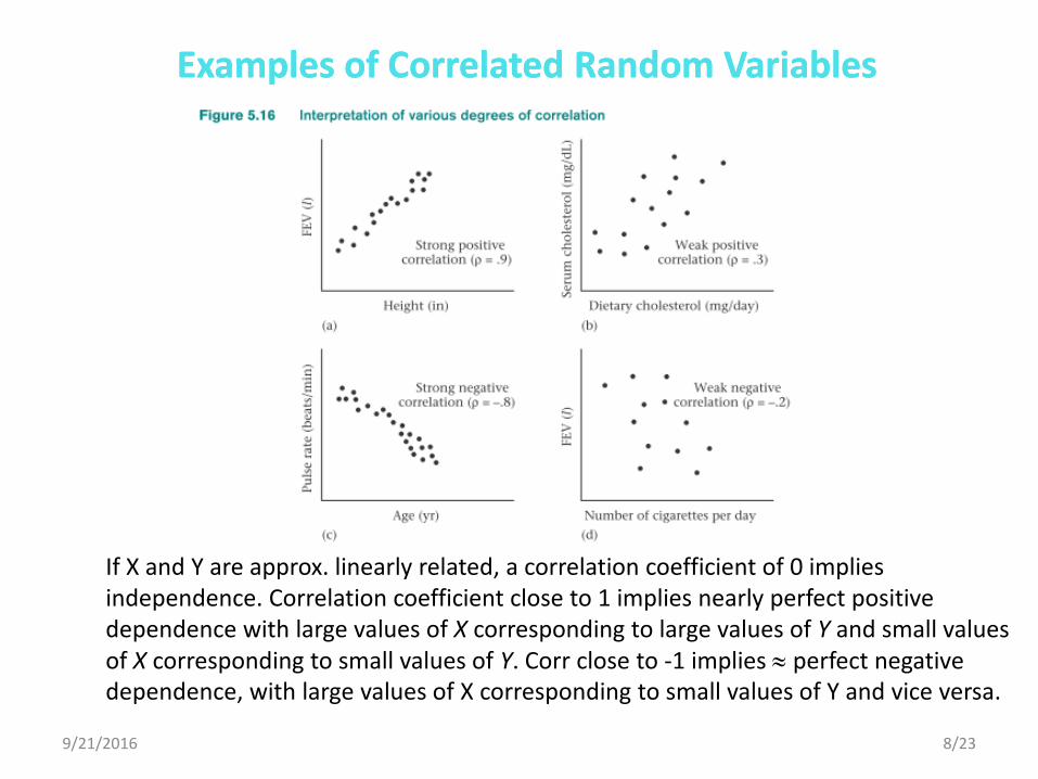
If X and Y are approx. linearly related, a correlation coefficient of 0 implies independence. Correlation coefficient close to 1 implies nearly perfect positive dependence with large values of X corresponding to large values of Y and small values of X corresponding to small values of Y. Corr close to -1 implies perfect negative dependence, with large values of X corresponding to small values of Y and vice versa.

Examples of Correlated Random VariablesExamples of Correlated Random Variables

9/21/2016 8/23

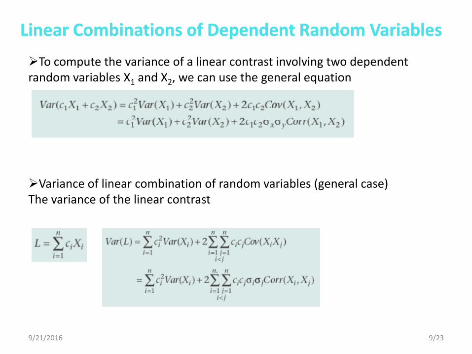
To compute the variance of a linear contrast involving two dependent random variables X1 and X2, we can use the general equation

Variance of linear combination of random variables (general case) The variance of the linear contrast

Linear Combinations of Dependent Random VariablesLinear Combinations of Dependent Random Variables

9/21/2016 9/23

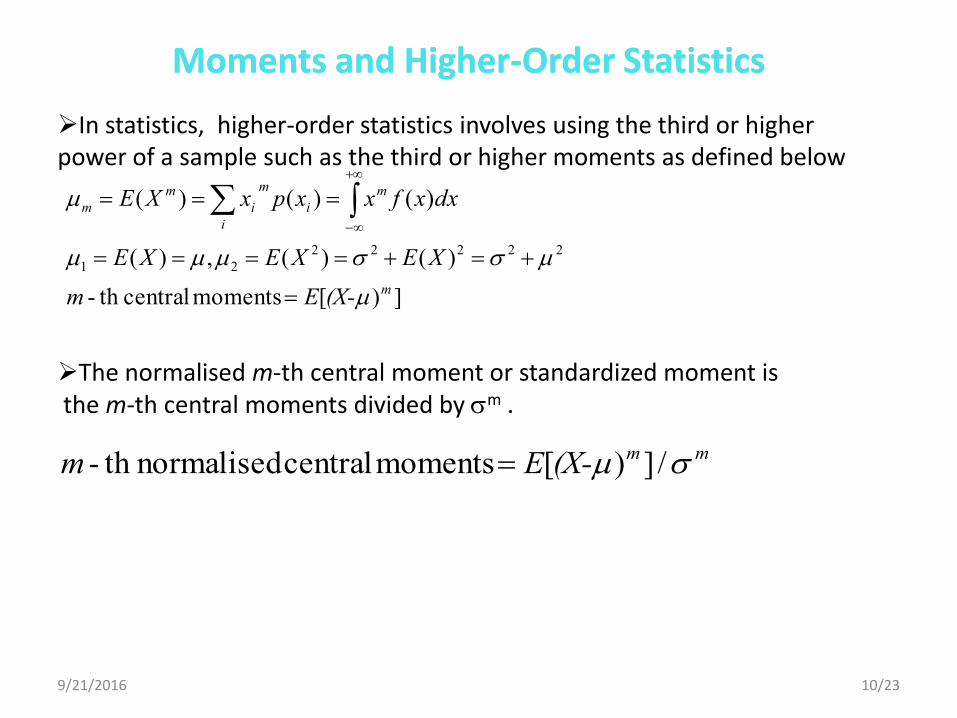
In statistics, higher-order statistics involves using the third or higher power of a sample such as the third or higher moments as defined below

The normalised m-th central moment or standardized moment is the m-th central moments divided by m .

Moments and HigherMoments and Higher--Order StatisticsOrder Statistics

9/21/2016

])[ moments centralth -

)()(,)(

)()()(

22222

21

m

m

i

m

i

i

m

m

(X-Em

XEXEXE

dxxfxxpxXE

mm(X-Em /])[ moments central normalisedth -

10/23

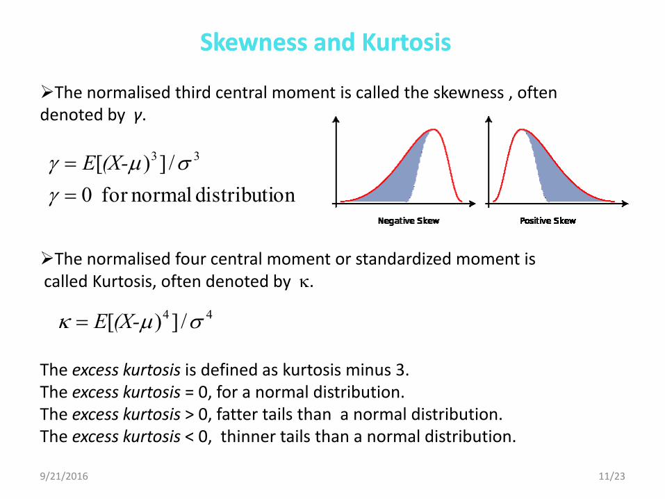
The normalised third central moment is called the skewness , often denoted by γ.

The normalised four central moment or standardized moment is called Kurtosis, often denoted by . The excess kurtosis is defined as kurtosis minus 3. The excess kurtosis = 0, for a normal distribution. The excess kurtosis > 0, fatter tails than a normal distribution. The excess kurtosis < 0, thinner tails than a normal distribution.

SkewnessSkewness and Kurtosisand Kurtosis

9/21/2016

44 /])[ (X-E

ondistributi normalfor 0

/])[ 33

(X-E

11/23

Sampling DistributionSampling Distribution

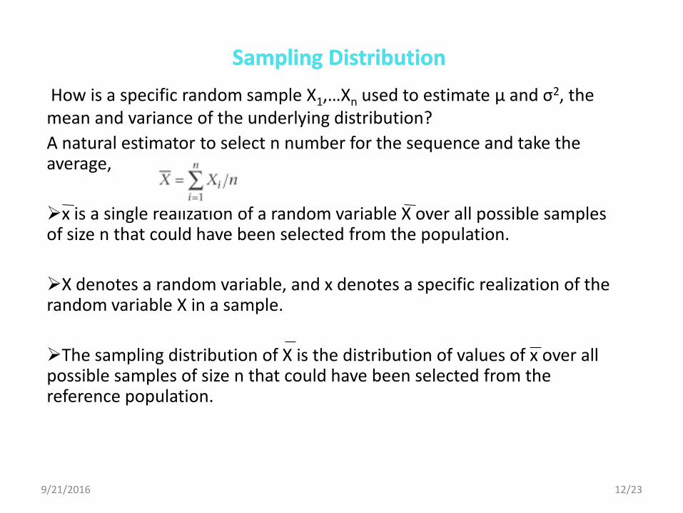
How is a specific random sample X1,…Xn used to estimate μ and σ2, the mean and variance of the underlying distribution?

A natural estimator to select n number for the sequence and take the average,

x is a single realization of a random variable X over all possible samples of size n that could have been selected from the population.

X denotes a random variable, and x denotes a specific realization of the random variable X in a sample.

The sampling distribution of X is the distribution of values of x over all possible samples of size n that could have been selected from the reference population.

9/21/2016 12/23

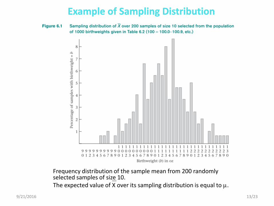
Frequency distribution of the sample mean from 200 randomly selected samples of size 10. The expected value of X over its sampling distribution is equal to .

Example of Sampling Distribution Example of Sampling Distribution

9/21/2016 13/23

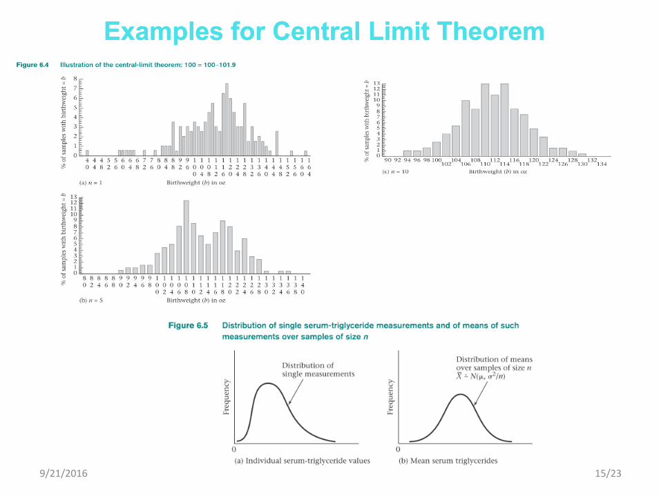
Let X1, …, Xn be a random sample from some population with mean and variance 2. Then for large n, X N(, 2/n) even if the underlying distribution of individual observations in the population is not normal. (The symbol is used to represent “approximately distributed.)

This theorem allows us to perform statistical inference based on the approximate normality of the sample mean despite the nonnormality of the distribution of individual observations.

The skewness of the distribution can be reduced by transformation data using log scale. The central-limit theorem can them be applicable for smaller sizes than if the data are retained in the original scale.

Central Limit TheoremCentral Limit Theorem

9/21/2016 14/23

~

~

Examples for Central Limit TheoremExamples for Central Limit Theorem

9/21/2016 15/23

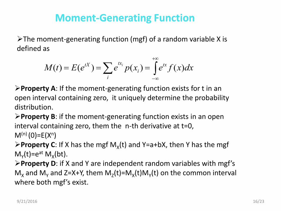
The moment-generating function (mgf) of a random variable X is defined as

Property A: If the moment-generating function exists for t in an open interval containing zero, it uniquely determine the probability distribution. Property B: if the moment-generating function exists in an open interval containing zero, them the n-th derivative at t=0, M(n) (0)=E(Xn) Property C: If X has the mgf MX(t) and Y=a+bX, then Y has the mgf MY(t)=eat MX(bt). Property D: if X and Y are independent random variables with mgf’s MX and MY and Z=X+Y, them MZ(t)=MX(t)MY(t) on the common interval where both mgf’s exist.

MomentMoment--Generating FunctionGenerating Function

9/21/2016

dxxfexpeeEtM tx

i

tx

i

tX i

)()()()(

16/23

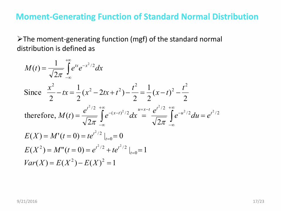
The moment-generating function (mgf) of the standard normal distribution is defined as

MomentMoment--Generating Function of Standard Normal Distribution Generating Function of Standard Normal Distribution

9/21/2016

1)()()(

1|)0(")(

0|)0(')(

22)( therefore,

2)(

2

1

2)2(

2

1

2 Since

2

1)(

22

0

2/2/2

0

2/

2/2/2/

2/)(2/

22

222

2

2/

22

2

22

2

2

2

2

XEXEXVar

teetMXE

tetMXE

eduee

dxee

tM

ttx

tttxxtx

x

dxeetM

t

tt

t

t

tuttxu

txt

xtx

17/23

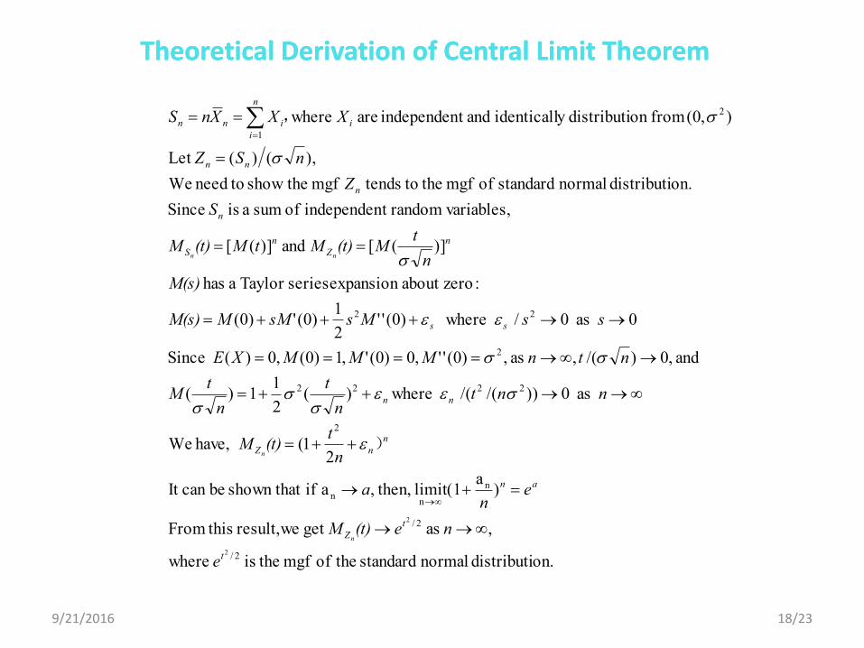
Theoretical Derivation of Central Limit TheoremTheoretical Derivation of Central Limit Theorem

9/21/2016

on.distributi normal standard theof mgf theis where

, as get weresult, thisFrom

)a

(1limit then,,a if shown that becan It

21( have, We

as 0))/(/( where)(2

11)(

and ,0)/(, as ,)0('',0)0(',1)0(,0)( Since

0 as 0/ where)0(''2

1)0(')0(

:zeroabout expansion seriesTaylor a has

)]([ and )]([

, variablesrandomt independen of sum a is Since

on.distributi normal standard of mgf the to tends mgf theshow toneed We

),()(Let

),0( fromon distributiy identicall andt independen are where

2/

2/

n

nn

2

22

22

2

2

2

2

1

2

2

t

t

Z

an

n

nZ

nn

ss

n

Z

n

S

n

n

nn

i

n

i

inn

e

ne(t)M

en

a

n

t(t)M

nntn

t

n

tM

ntnMMMXE

ssMssMMM(s)

M(s)

n

tM(t)MtM(t)M

S

Z

nSZ

XXXnS

n

n

nn

）

，

18/23

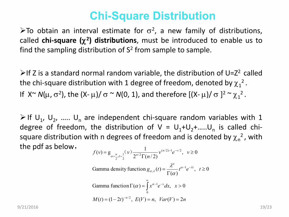
To obtain an interval estimate for 2, a new family of distributions, called chi-square (2) distributions, must be introduced to enable us to find the sampling distribution of S2 from sample to sample.

If Z is a standard normal random variable, the distribution of U=Z2 called the chi-square distribution with 1 degree of freedom, denoted by 1

2 .

If X~ N(, 2), the (X- )/ ~ N(0, 1), and therefore [(X- )/ ]2 ~ 12 .

If U1, U2, ….. Un are independent chi-square random variables with 1

degree of freedom, the distribution of V = U1+U2+…..Un is called chi-square distribution with n degrees of freedom and is denoted by n

2 , with the pdf as below，

ChiChi--Square DistributionSquare Distribution

nVVarnVEttM

xdxex

tettg

vevn

vvf

n

x

t

vn

nn

2)( ,)( ,)21()(

0 ,)(function Gamma

0 ,)(

)(function density Gamma

0 ,)2/(2

1g)(

2/

0

1

1

,

2/1)2/(

2/

2

1,

2

）（

9/21/2016 19/23

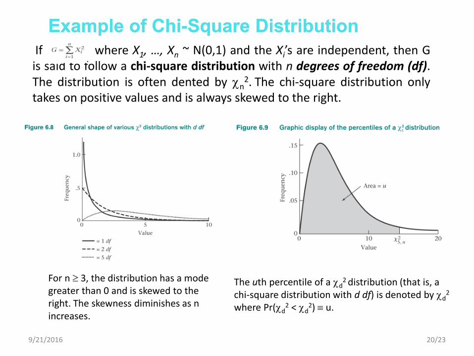
If where X1, …, Xn ~ N(0,1) and the Xi’s are independent, then G is said to follow a chi-square distribution with n degrees of freedom (df). The distribution is often dented by n

2. The chi-square distribution only takes on positive values and is always skewed to the right.

Example of Example of ChiChi--Square DistributionSquare Distribution

For n 3, the distribution has a mode greater than 0 and is skewed to the right. The skewness diminishes as n increases.

The uth percentile of a d2 distribution (that is, a

chi-square distribution with d df) is denoted by d2

where Pr(d2 < d

2) u.

9/21/2016 20/23

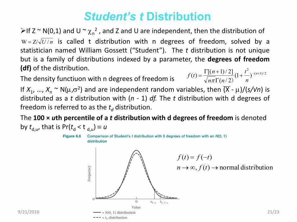
If Z ~ N(0,1) and U ~ n2 , and Z and U are independent, then the distribution of

is called t distribution with n degrees of freedom, solved by a statistician named William Gossett (“Student”). The t distribution is not unique but is a family of distributions indexed by a parameter, the degrees of freedom (df) of the distribution.

The density functiuon with n degrees of freedom is

If X1, …, Xn ~ N(,2) and are independent random variables, then (X - )/(s/√n) is distributed as a t distribution with (n - 1) df. The t distribution with d degrees of freedom is referred to as the td distribution.

The 100 × uth percentile of a t distribution with d degrees of freedom is denoted by td,u, that is Pr(td < t d,u) u

Student’s tStudent’s t DistributionDistribution

nU /Z/W

2/)1(2

)1(2/(

]2/)1[()(

n

n

t

nn

ntf

）

ondistributi normal )(,

)()(

tfn

tftf

9/21/2016 21/23

Let U and V be independent chi-square random variables with m and n degrees of freedom respectively. The distribution of a new random variable W=(U/m)/(V/n) is called the F distribution with m and n degrees of freedom and is denoted by Fm,n, with the density function as

F F DistributionDistribution

0 ,)m

1()m

()2/)2/(

]2/)[()( 2/)(12/2/

ww

nw

nnm

nmwf nmmm

（

9/21/2016 22/23

Summary

In this chapter, we discussed

Expected and variance of functions of random variables

Moment generating function

Central-limit theorem

Three distributions from the normal distribution

t, chi-square, and F distributions

9/21/2016 23/23

The End

9/21/2016 24/23