FISH 437/537Fisheries Oceanography

January 30, 2009

Bio-Physical Coupling in Fisheries Oceanography – A

biological oceanographer’s view

Jeffrey NappNOAA – Fisheries

Alaska Fisheries Science Center

Definitions

• Autecology-

• Synecology-

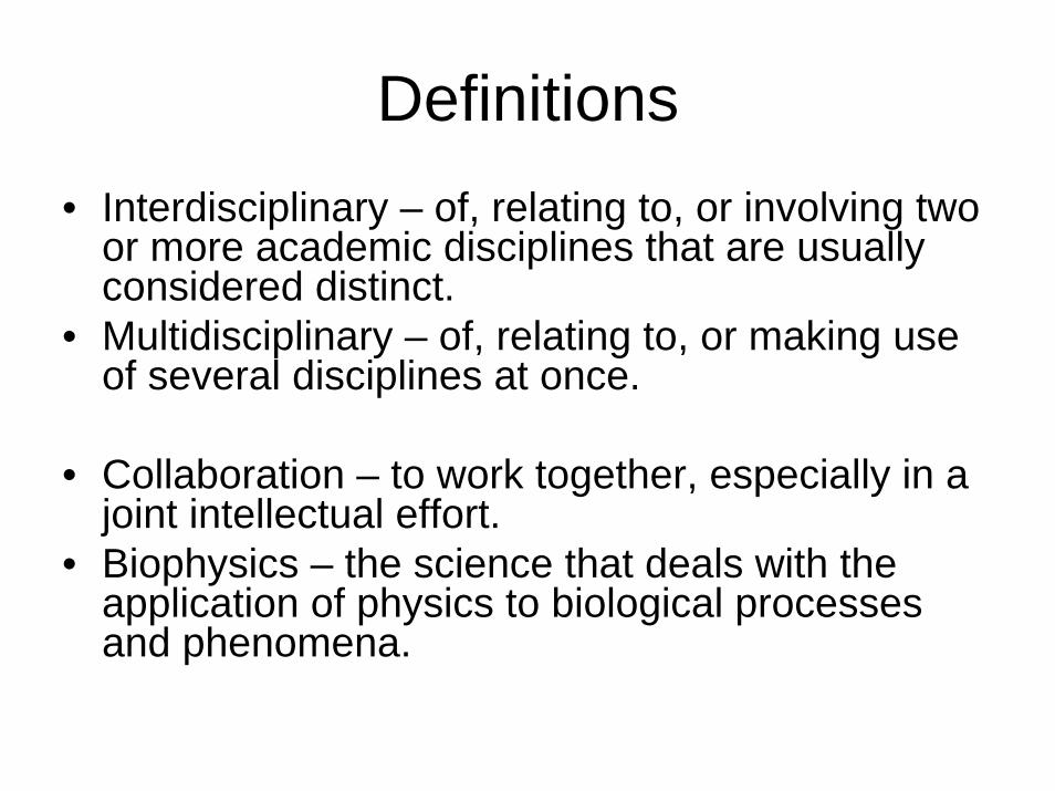
Definitions• Interdisciplinary – of, relating to, or involving two

or more academic disciplines that are usually considered distinct.

• Multidisciplinary – of, relating to, or making use of several disciplines at once.

• Collaboration – to work together, especially in a joint intellectual effort.

• Biophysics – the science that deals with the application of physics to biological processes and phenomena.

Is It Fisheries or Biological Oceanography?

“Biological Oceanography is concerned with the interactions of populations of marine organisms with one another and with their physical and chemical environment. Because these interactions are frequently complex, and because the concepts and techniques used are drawn from many fields, biological oceanography is, of necessity, interdisciplinary. Therefore, studies in physical oceanography, marine chemistry, and marine geology, and several biological areas are pertinent.”

SIO Graduate Department (http://scrippseducation.ucsd.edu/Graduate_

Students/PhD_Program/Specializations/Biological_Oceanography/)

Summary of Process to Conduct Biophysical Coupling Projects

• Define your questions• Identify mechanisms or paradigm• Identify key variables (include potential

interactions)• Identify necessary expertise (collaborate?)• Conduct a trial or pilot study• Refine approach• Do It!

Start with a Paradigm, Hypothesis or Set of Mechanisms

Biophysical Factors Influencing GOA Walleye Pollock Recruitment

Are There Competing Paradigms? Complexity & Fish Recruitment

Recruitment of Populations &

Stocks

Activating Factors Constraining Factors(Stochastic Impact) (Deterministic Impact)

High γ environmentTurbulencePrey availabilityAdvectionPlanktonic and

migratory predatorsIntra-cohort density

processes

Low γ effectsLong-lived predatorsPhysical barriersAdaptationsHabitat sizeInter-cohort density

processesCommunity structure

Bailey et al., (2005) Prog. Oceanogr. 67: 24 - 42

Recruitment of Populations &

Stocks

Activating Factors Constraining Factors(Stochastic Impact) (Deterministic Impact)

Example # 1 -- Larval Fish Feeding

Feeding = f (what variables)

• Size & development of larva

• Past feeding (hunger)

• Prey density

• Available prey (susceptibility todetection & capture, nutritionalcondition)

• Light (season, cloud cover)

• Temperature (large & small scalepatterns in solar radiation)

• Small-scale turbulence (wind, watercolumn stability)

• Water turbidity / clarity (biologicalproduction, sediments)

• Interactions among variables

Problem: General lack of field studies that quantitatively address the potential interactions among environmental covariates that affect larval fish feeding.

Objective: Explain variability of in situ feeding of larval walleye pollock

Tool: Generalized Additive Models (GAM) to allow the inclusion of non-additive effects.

Porter, S. et al., 2005. MEPS 302:207-217.

Partial Additive Effects of VariablesPositive effect on feeding

Negative effect on feeding

R2 = 0.82w/o interactions

R2 = 0.89w. interactions

Conclusion: Effect of turbulence cannot be

determined in isolation, but is dependent on the

amount of light.

Interaction of Light & Wind

Mechanism: both larvae and their prey are moving deeper in the water column to avoid turbulence. Results in concentration of prey, but requires higher incident light levels to see prey at these greater depths.

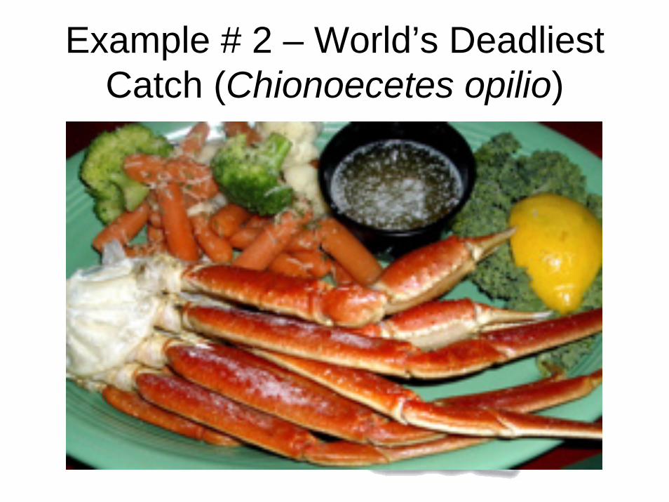
Example # 2 – World’s Deadliest Catch (Chionoecetes opilio)

Contraction and shift of geographic range of snow crab

Eastern Bering Sea Shelf Structure

?

• Female snow crab distribution has shifted and contracted to the northwestern parts of the Eastern Bering Sea (EBS)

• This coincides with warming of near bottom temperatures over the EBS, and reduction of the “Cold Pool”

S. Hinckley, C. Parada, D. Armstrong, L. Orensanz, B. Ernst, J. Horne, B. Megrey, J. Napp

Important Variables / Mechanisms

• Spatial distributions (females, prey, predators)

• Advection (rates, water column shear)• Planktonic duration (development,

temperature)• Mortalities during planktonic phase• Optimal nursery habitat (temperature)

Snow crab conceptual model

Release time Settlement time

Upward larval movement

Mixed layer

Release areas Bottom layer Settlement areas

Early juvenile settlement

Horizontal advection and vertical maintenance around this layer

3 months

2 months

Time

1th April 1th June 1th July 1th October

space

• Couple a hydrodynamic model and an individual-based model to study the transport of crab larvae from release to potential settlement areas in Bering Sea

Methodological approach

ROMS Crab IBM

Winds

Temperature

Atmosphericheat

Currents

Freshwaterfluxes

Salinity Particle positionsHydrodynamic model

Individual-based model

forcings

inputs

Temperatureat settlement

GIS

Number ofsettlers

Connectivitymatrix

Statisticalanalysis

Visualizationandanimations

outputs

analysis

• Spatial Release:8 historical distribution areasMiddle and outer domainDepth: Vertical release at the bottom

• Temporal Release: 2 months between • 1st April and 1st June

• Settlement: 90 days after release

• Simulations• Larvae were released in the areas randomly during the release

period• For all years the same initial conditions were used.• The physical environment was representative of years 1978-2003

(from ROMS model).• Once larvae are released, they migrate vertically to the mixed layer

where stay until settlement period. • Trajectories to settlement were followed.

0 1

23

45

769

8

1011

1213

14

15

16Model Configuration

Connectivity Results

Retention Area

> 50%

25-50 %

10-25 %

Climate & Optimal Nursery Areas

1978 1979 1980 1981 1982

1983 1984 1985 1986 1987

1988 1989 1990 1991 1992

1993 1994 1995 1996 1997

1999 2000 200220011998

0-2oC

2-4oC

>4oC

< 0oC

Warm years

Cold years

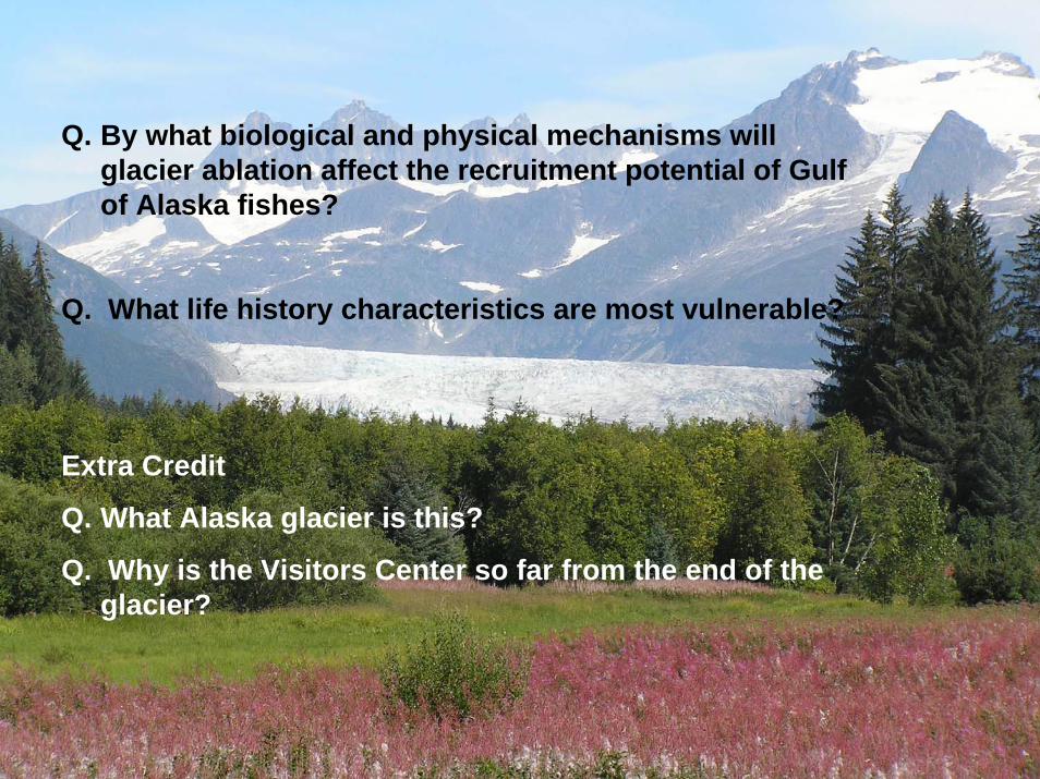
Q. By what biological and physical mechanisms will glacier ablation affect the recruitment potential of Gulf of Alaska fishes?

Q. What life history characteristics are most vulnerable?

Extra Credit

Q. What Alaska glacier is this?

Q. Why is the Visitors Center so far from the end of the glacier?

Summary of Process to Conduct Biophysical Coupling Projects

• Define your questions• Identify mechanisms or paradigm• Identify key variables (consider potential

interactions)• Identify necessary expertise (collaborate?)• Conduct a trial or pilot study• Refine approach• Do It!

“Operational” Biophysical Fisheries Oceanography – How to Find a

Partner (E-harmony)• Well respected in their own field; gives and

gets respect• Not over-committed• Open to thinking in a new way• A good teacher; tolerant, flexible• Enthusiastic• Open to challenges from peers

(assumptions and conclusions)

How To Prepare Yourself To Be An Exceptional Partner

• Become multi-disciplinary• Take oceanography classes• Acquire advanced quantitative skills• Learn to show your enthusiasm – it’s

contagious• Learn as much as you can about your

collaborator’s fields

Example #3 – Eastern Bering Sea Walleye Pollock

• GOA (2008) -161,000 t

• Bogoslof Is. (2007) –290,000 t

• EBS (2009) –1,443,000 t

SpawningAdults Eggs Yolk sac

larvaeFeedinglarvae

Advection & Mesoscale Variability

EffectivePrey Concentration

Presence or Absence of Sea-Ice & Water Temperature

Wind Mixing/Turbulence

Timing of Preferred Prey Production

Oce

anic

Reg

ion

She

lfR

egio

n

Mechanisms

Napp et al., 2000 Fish. Oceanogr. 9: 147-162See more recent revisions by Hunt et al., 2008 & 2002

Transport – Role of Eddies-1

-1

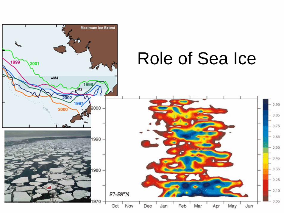
Role of Sea Ice

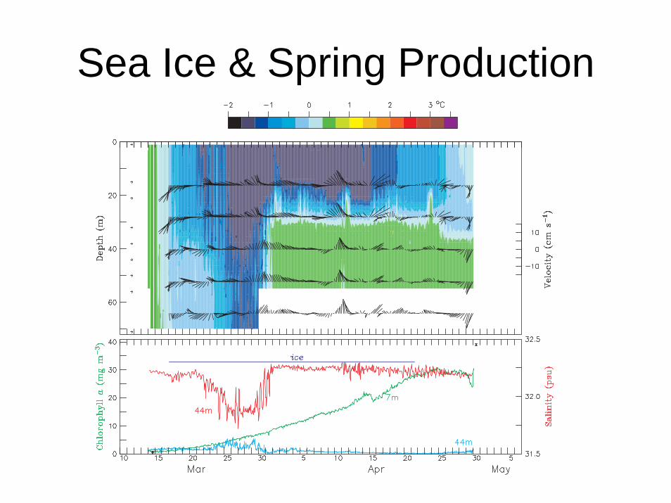
Sea Ice & Spring Production

Think ecosystems and biophysical coupling!

Adapted from S.A. Macklin, NOAA - PMEL