Binomial Distibutions

Target Goal:

I can determine if the conditions for a binomial random variable are met.

I can find the individual and cumulative binomial probabilities using the calculator.

6.3a

h.w: pg 381: 61, 65, 66; pg 403: 69, 71, 73

The Binomial Distribution

When we are studying situations with two possible outcomes we are interested in a binomial setting.

What are some outcomes with two possible outcomes?

Toss a coin Shoot a free throw Have a boy or a girl

Binomial Setting

Suppose the random variable X = the number of successes in n observations.

Then X is a binomial random variable if:

1. Binary: there are only two outcomes, success or failure.

2. There is a fixed number n of trials.

3. The n trials are independent.

4. The probability of success p is the same for each trial (observation).

If X is a binomial random variable, it is said to have a binomial distribution, and is denoted as

B(n, p) n: # of observations p: probability of success

A binomial distribution or not?

Blood Types

Parents carry genes O and A blood type. The probability a child gets two “O” genes is 0.25. If there are 5 children in a family, is each birth independent?

Yes, so X is the count of success

(“O” blood type), and

X is B(5, 0.25)

Dealing cards No. If you deal cards without replacement,

the next card is affected by the previous. Not independent.

Inspecting Switches In a shipment, 10 % of the switches are bad

(unknown to the inspector). If the engineer takes a SRS of 10 switches

from 10,000. The engineer counts X, the number of bad switches.

Is this Binomial?

Not quite binomial. Removing one changes the proportion of bad switches.

But, if the SRS is 10,000, removing one changes the remaining 9,999 very little.

When the population is much larger than the sample, we say the distribution is approximately binomial and very close to:

B(10,0.10)

Activity: A Gaggle of Girls How unusual is it for a family to have three

girls if the probability of having a boy and a girl is equally likely?

If success = girl and failure = boy, then p(success) = 0.5.0.5.

Define the random variable X as the number of girls.

We want to simulate families with three children.

Our goal is to determine the long term relative frequency of a family with 3 girls, P(X=3)

Using the Random Number Table D

1. Let the even digits represent “girl” and the odd digits represent “boy”.

Each student select their own row, and beginning at that row, read off numbers three at a time.

Each three digits will constitute one trail. Use tally marks to record the results of 40

trails which will then be pooled with the class.

Calculate the relative frequency of the event.

P(X=3) = /40 = vs. Class relative frequency:

3 girls 3 girls

Not 3 girls Not 3 girls

Using the Calculator

2. Using the codes 1 = girl and 0 = boy; Enter the command

math:prb:randint(0,1,3). This command instructs the calculator to

randomly pick a whole number from the set {0,1} and do this three times.

The outcome {0,0,1} represents {boy, boy, girl}.

Continue to press ENTER until you have 40 trails.

Use a tally mark to record each time a {1,1,1} result.

3 girls 3 girls

Not 3 girls Not 3 girls

Calculate the relative frequency of the event.

P(X=3) = /40 = vs. class relative frequency: Do the results of our simulation come close

to the theoretical value for P(X=3) which is 0.125?

Even quicker…Try

Math:PRB:randBin(#trials,prob,#of simulations) randBin(3,.5,40) store L1

(2 1 0 3 …); 3 is 3 girls or next, Sum(L1=3): count the # of 3 girl possibilities. It changes the 3’s to 1(true) and counts.

Finding Binomial Probabilities using the Calculator The probability distribution function(p.d.f.)

assigns a probability to each value of X.

P(X=2)

Calculator: TI-83:

2nd:VARS: binompdf (n, p, X)

Cumulative Distributions The cumulative distribution function(c.d.f.)

calculates the sum of the probabilities up to X.

P(X≤ 2) = P(X=0) + P(X=1) + P(X = 2)

Calculator: TI-83:

2nd:VARS: binomcdf (n, p, X)

Example: Glex’s Free Throws Over an entire season Glex shoots 75%

free throw percentage. She shoots 7/12 and the fans think she was nervous.

Is this unusual for Glex to shoot so poorly?

Studies of long series found no evidence that free throws are dependent so assume free throws are independent.

Probability of success = 0.75 X: The number of baskets made in 12

attempts. Find the probability of making at most 7

free throws.

B(n, p)

B(12, 0.75)

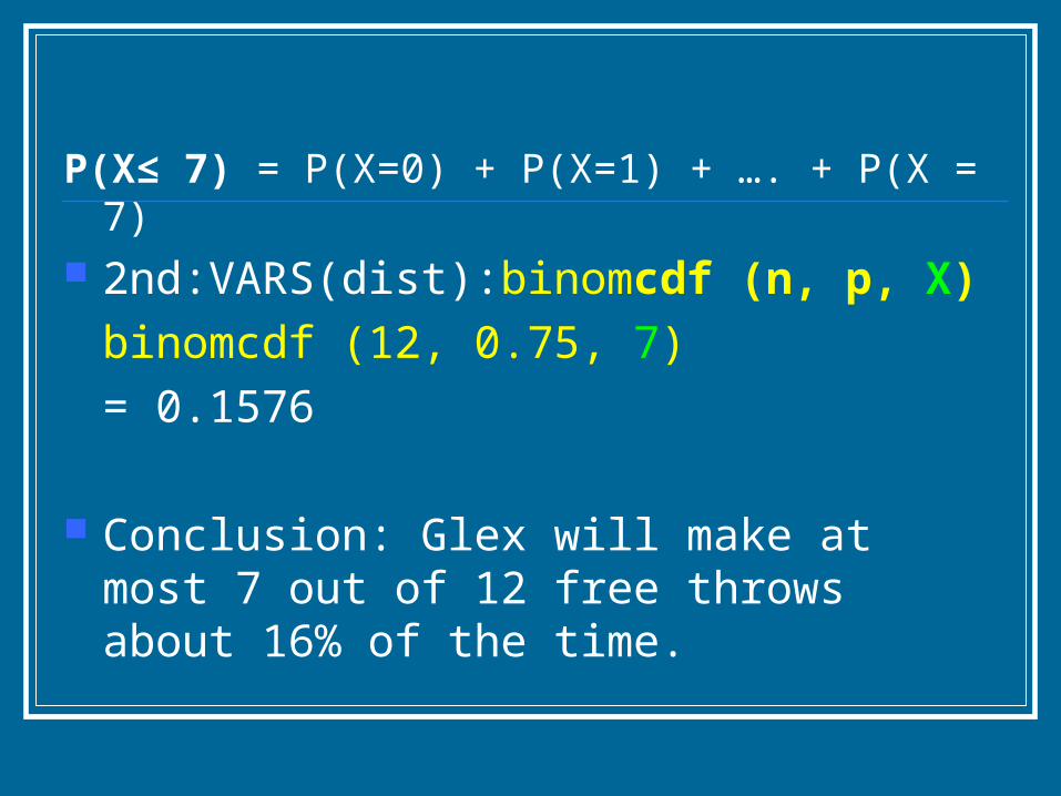
P(X≤ 7) = P(X=0) + P(X=1) + …. + P(X = 7) 2nd:VARS(dist):binomcdf (n, p, X)

binomcdf (12, 0.75, 7)

= 0.1576

Conclusion: Glex will make at most 7 out of 12 free throws about 16% of the time.

Example : Type O Blood Type Suppose each child born to John and Katie

has probability 0.25 of having blood type O. If John and Katie have 5 children, what is the probability that exactly 2 of them have type O blood?

Binomial distribution?

X: the number of children with type O blood.

Calculator: TI-83: binompdf(n, p, X) Note: binompdf ( 5, 0.25, 0) = 0.2373, finds

the P(X=0), none of the children have type O blood.

TI-89: tistat.binomPdf(n, p, X)

Calculator Procedure: Enter values of x; 0, 1, 2, 3, 4, 5 into L1

Enter the binomial probabilities into L2. Highlight L2 and enter 2nd:VARS(dist):

binompdf (5, 0.25, L1). Fill in table. (2 min)

What is the probability that exactly 2 of them have type O blood?

P(X=2) = 0.2637

XX 00 11 22 33 44 55

P(X) P(X) 0.2370.2373 3

0.3950.39555

0.2630.26377

0.0870.08799

0.0140.01466

0.000.0011

Plot a histogram of the binomial pdf.

Deselect or delete active functions in Y = window.

Define Plot1 to be a histogram with Xlist: L1, Freq: L2

Set the window X[0, 6]1 and Y[0, 1]0.1

Use the TRACE button to inspect the heights of the bars.

Verify that the sum of the probabilities is 1.

STAT:CALC:1-VAR Stats L2

Fill in the following table of the cumulative distribution function (c.d.f.) for the binomial random variable, X.

To calculate cumulative probabilities: Highlight L3 and enter

2nd:VARS(dist): binomcdf (5, 0.25, L1).

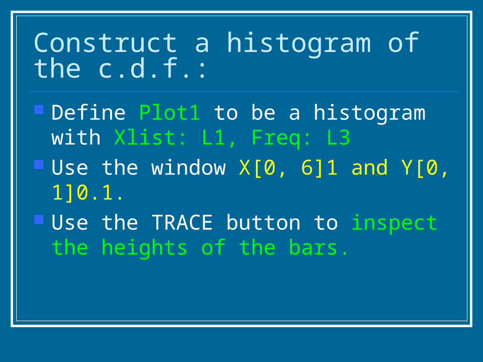
Construct a histogram of the c.d.f.:

Define Plot1 to be a histogram with Xlist: L1, Freq: L3

Use the window X[0, 6]1 and Y[0, 1]0.1. Use the TRACE button to inspect the

heights of the bars.

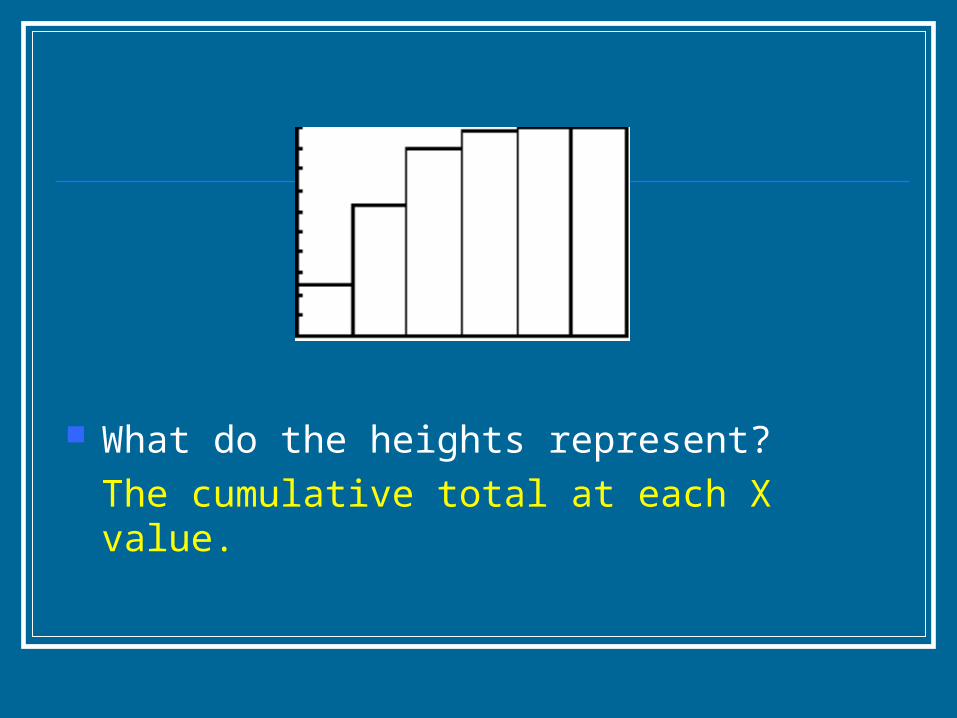
What do the heights represent?

The cumulative total at each X value.

Compare: p.d.f.

c.d.f.

Note: Binomcdf ( 5, 0.25, 1) = 0.6328

XX 00 11 22 33 44 55

P(X)P(X) 0.2370.2373 3

0.3950.39555

0.26370.2637 0.0870.08799

0.0140.01466

0.000.0011

F(X) F(X) 0.2370.237

3 3 0.6320.632

88 0.89650.8965 0.9840.984

44 0.9840.984

44 11

( 0)P X ( 1)P X ( 2)P X ( 3)P X ( 4)P X ( 5)P X