Embed Size (px)
Citation preview
School of Informatics, University of Edinburgh
System 6 Introduction
Is there a Wedge in this 3D scene?
Data a stereo pair of images!
AV: 3D recognition from binocular stereo Fisher lecture 6 slide 1
School of Informatics, University of Edinburgh
Binocular Stereo Vision
Given two 2D images of an object, how can wereconstruct 3D awareness of it?
AV: 3D recognition from binocular stereo Fisher lecture 6 slide 2
School of Informatics, University of Edinburgh
Stereo vision - a solution
1) Feature extraction
2) Feature matching:
3) Triangulation:
AV: 3D recognition from binocular stereo Fisher lecture 6 slide 3
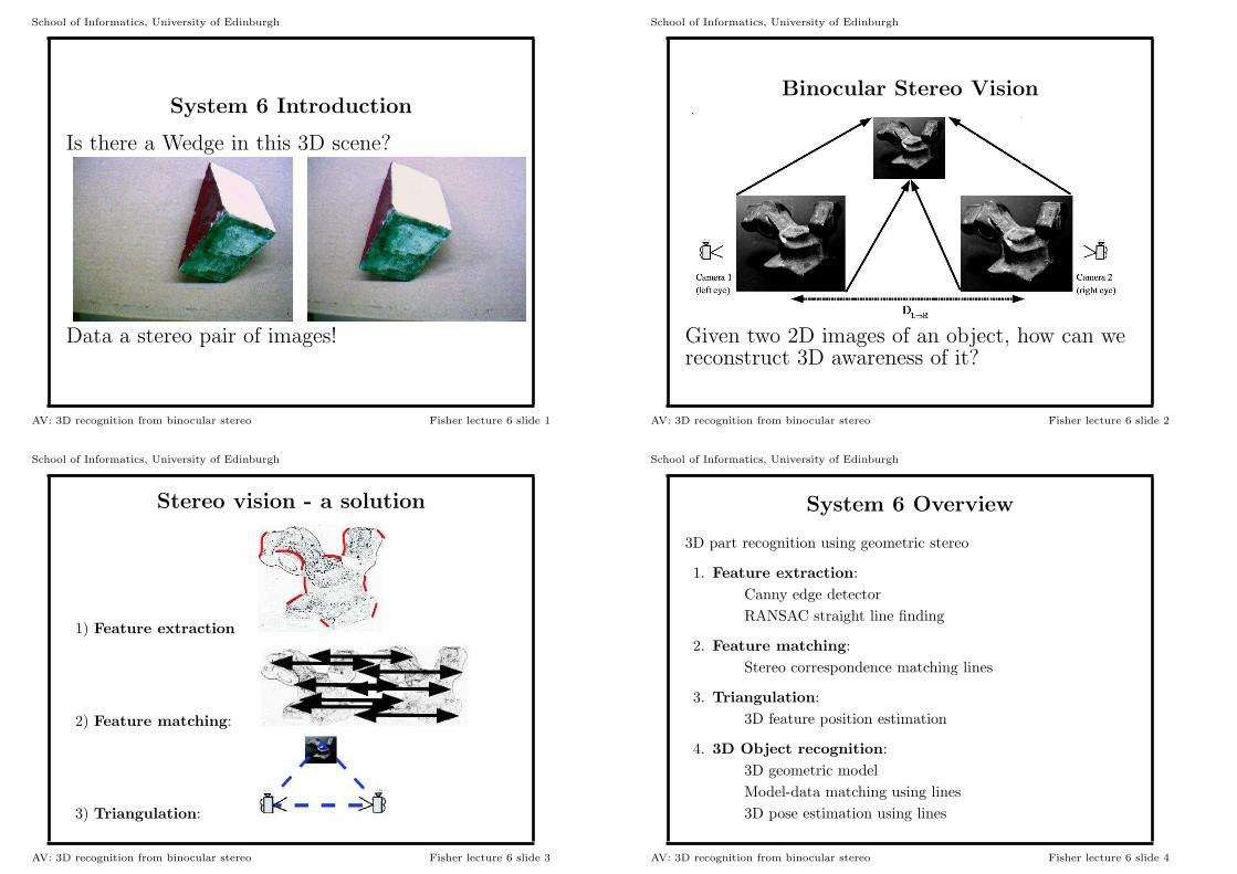
School of Informatics, University of Edinburgh
System 6 Overview
3D part recognition using geometric stereo
1. Feature extraction:
Canny edge detector
RANSAC straight line finding
2. Feature matching:
Stereo correspondence matching lines
3. Triangulation:
3D feature position estimation
4. 3D Object recognition:
3D geometric model
Model-data matching using lines
3D pose estimation using lines
AV: 3D recognition from binocular stereo Fisher lecture 6 slide 4
School of Informatics, University of Edinburgh
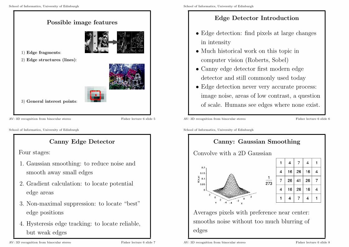
Possible image features
1) Edge fragments:
2) Edge structures (lines):
3) General interest points:
AV: 3D recognition from binocular stereo Fisher lecture 6 slide 5
School of Informatics, University of Edinburgh
Edge Detector Introduction
• Edge detection: find pixels at large changes
in intensity
• Much historical work on this topic in
computer vision (Roberts, Sobel)
• Canny edge detector first modern edge
detector and still commonly used today
• Edge detection never very accurate process:
image noise, areas of low contrast, a question
of scale. Humans see edges where none exist.
AV: 3D recognition from binocular stereo Fisher lecture 6 slide 6
School of Informatics, University of Edinburgh
Canny Edge Detector
Four stages:
1. Gaussian smoothing: to reduce noise and
smooth away small edges
2. Gradient calculation: to locate potential
edge areas
3. Non-maximal suppression: to locate “best”
edge positions
4. Hysteresis edge tracking: to locate reliable,
but weak edges
AV: 3D recognition from binocular stereo Fisher lecture 6 slide 7
School of Informatics, University of Edinburgh
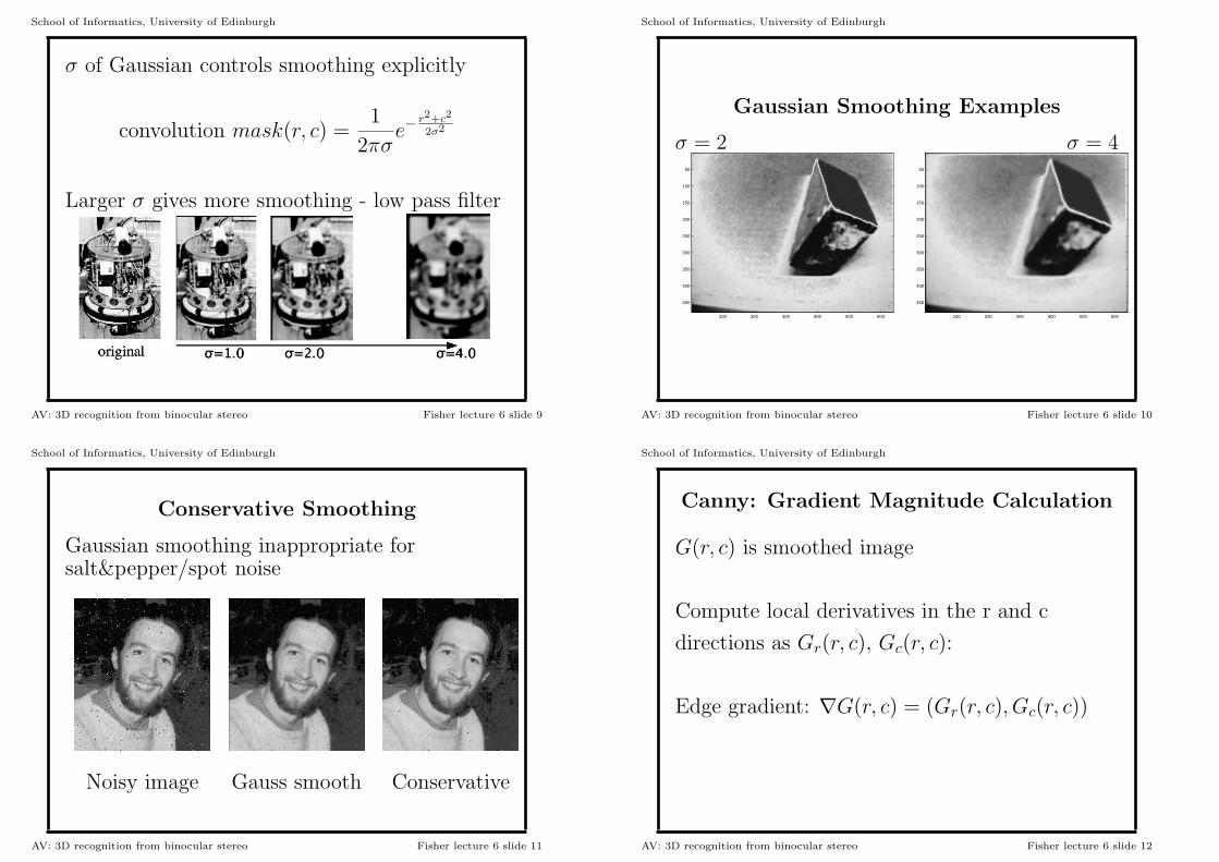
Canny: Gaussian Smoothing
Convolve with a 2D Gaussian
Averages pixels with preference near center:
smooths noise without too much blurring of
edges
AV: 3D recognition from binocular stereo Fisher lecture 6 slide 8
School of Informatics, University of Edinburgh
σ of Gaussian controls smoothing explicitly
convolution mask(r, c) =1
2πσe−
r2+c2
2σ2
Larger σ gives more smoothing - low pass filter
AV: 3D recognition from binocular stereo Fisher lecture 6 slide 9
School of Informatics, University of Edinburgh
Gaussian Smoothing Examples
σ = 2 σ = 4
100 200 300 400 500 600
50
100
150
200
250
300
350
400
450
100 200 300 400 500 600
50
100
150
200
250
300
350
400
450
AV: 3D recognition from binocular stereo Fisher lecture 6 slide 10
School of Informatics, University of Edinburgh
Conservative Smoothing
Gaussian smoothing inappropriate forsalt&pepper/spot noise
Noisy image Gauss smooth Conservative
AV: 3D recognition from binocular stereo Fisher lecture 6 slide 11
School of Informatics, University of Edinburgh
Canny: Gradient Magnitude Calculation
G(r, c) is smoothed image
Compute local derivatives in the r and c
directions as Gr(r, c), Gc(r, c):
Edge gradient: ∇G(r, c) = (Gr(r, c), Gc(r, c))
AV: 3D recognition from binocular stereo Fisher lecture 6 slide 12
School of Informatics, University of Edinburgh
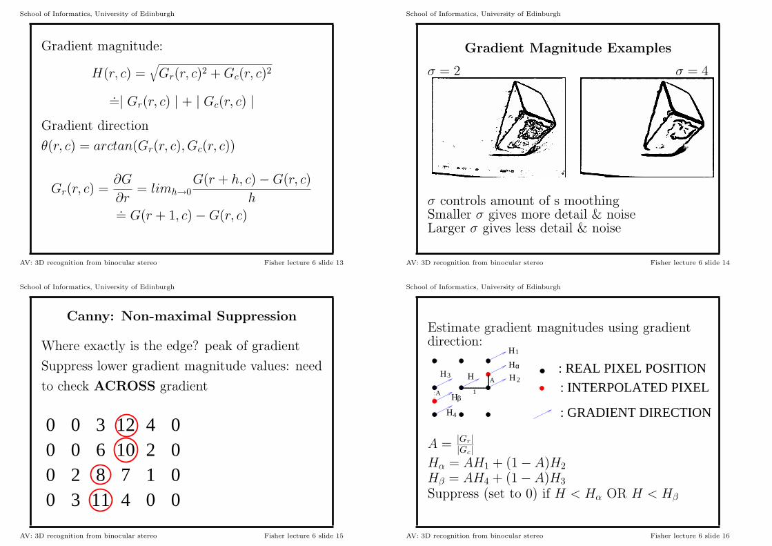
Gradient magnitude:
H(r, c) =√
Gr(r, c)2 + Gc(r, c)2
.=| Gr(r, c) | + | Gc(r, c) |
Gradient direction
θ(r, c) = arctan(Gr(r, c), Gc(r, c))
Gr(r, c) =∂G
∂r= limh→0
G(r + h, c) − G(r, c)
h.= G(r + 1, c) − G(r, c)
AV: 3D recognition from binocular stereo Fisher lecture 6 slide 13
School of Informatics, University of Edinburgh
Gradient Magnitude Examples
σ = 2 σ = 4
σ controls amount of s moothingSmaller σ gives more detail & noiseLarger σ gives less detail & noise
AV: 3D recognition from binocular stereo Fisher lecture 6 slide 14
School of Informatics, University of Edinburgh
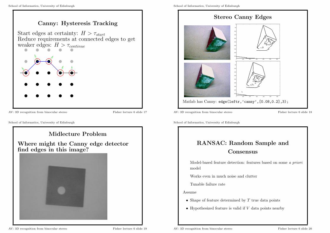
Canny: Non-maximal Suppression
Where exactly is the edge? peak of gradient
Suppress lower gradient magnitude values: need
to check ACROSS gradient
0 0 3 12 4 0000
0 00003
6 10 22 8 7 1
11 4
AV: 3D recognition from binocular stereo Fisher lecture 6 slide 15
School of Informatics, University of Edinburgh
Estimate gradient magnitudes using gradientdirection:
H4
3H H
H
H
H
1
2
α
A
A
1
: GRADIENT DIRECTION
: INTERPOLATED PIXELHβ
: REAL PIXEL POSITION
A = |Gr||Gc|
Hα = AH1 + (1 − A)H2
Hβ = AH4 + (1 − A)H3
Suppress (set to 0) if H < Hα OR H < Hβ
AV: 3D recognition from binocular stereo Fisher lecture 6 slide 16
School of Informatics, University of Edinburgh
Canny: Hysteresis Tracking
Start edges at certainty: H > τstartReduce requirements at connected edges to getweaker edges: H > τcontinue
AV: 3D recognition from binocular stereo Fisher lecture 6 slide 17
School of Informatics, University of Edinburgh
Stereo Canny Edges
0 100 200 300 400 500 600
0
50
100
150
200
250
300
350
400
450
0 100 200 300 400 500 600
0
50
100
150
200
250
300
350
400
450
Matlab has Canny: edge(leftr,’canny’,[0.08,0.2],3);
AV: 3D recognition from binocular stereo Fisher lecture 6 slide 18
School of Informatics, University of Edinburgh
Midlecture Problem
Where might the Canny edge detectorfind edges in this image?
AV: 3D recognition from binocular stereo Fisher lecture 6 slide 19
School of Informatics, University of Edinburgh
RANSAC: Random Sample and
Consensus
Model-based feature detection: features based on some a priori
model
Works even in much noise and clutter
Tunable failure rate
Assume
• Shape of feature determined by T true data points
• Hypothesized feature is valid if V data points nearby
AV: 3D recognition from binocular stereo Fisher lecture 6 slide 20
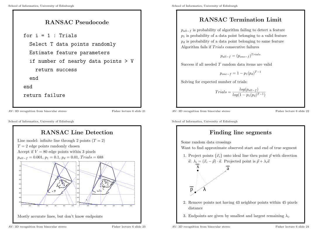
School of Informatics, University of Edinburgh
RANSAC Pseudocode
for i = 1 : Trials
Select T data points randomly
Estimate feature parameters
if number of nearby data points > V
return success
end
end
return failure
AV: 3D recognition from binocular stereo Fisher lecture 6 slide 21
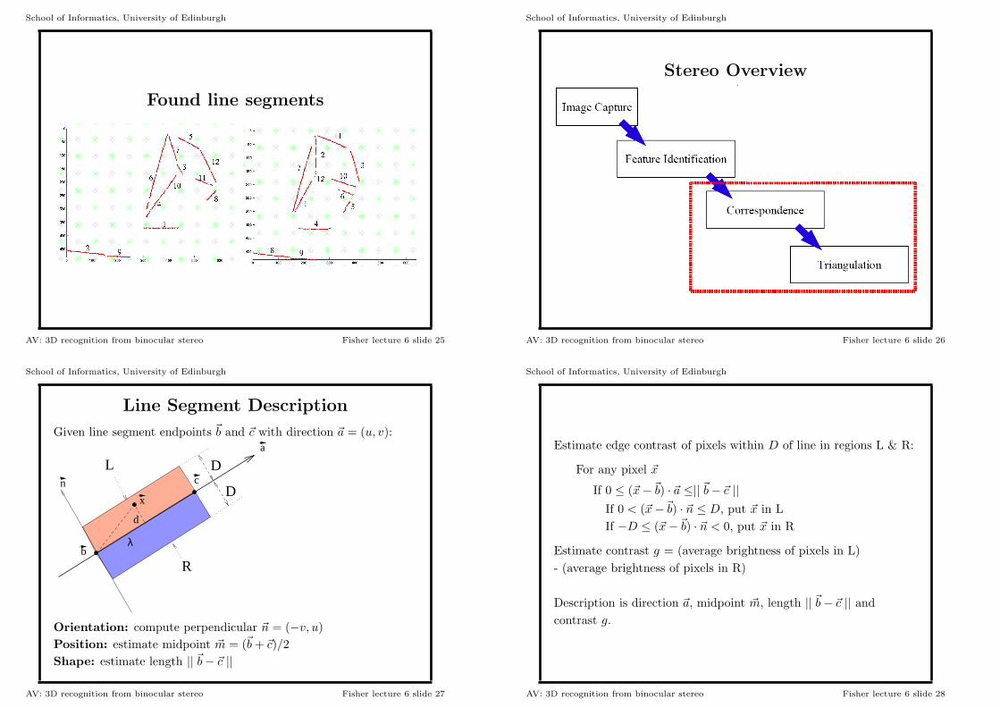
School of Informatics, University of Edinburgh
RANSAC Termination Limit
pall−f is probability of algorithm failing to detect a feature
p1 is probability of a data point belonging to a valid feature
pd is probability of a data point belonging to same feature
Algorithm fails if Trials consecutive failures
pall−f = (pone−f )Trials
Success if all needed T random data items are valid
pone−f = 1 − p1(pd)T−1
Solving for expected number of trials:
Trials =log(pall−f )
log(1 − p1(pd)T−1)
AV: 3D recognition from binocular stereo Fisher lecture 6 slide 22
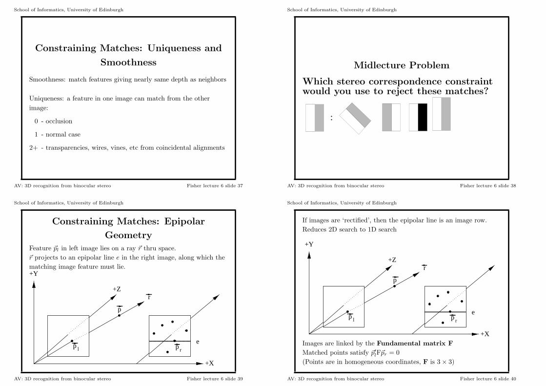
School of Informatics, University of Edinburgh
RANSAC Line Detection
Line model: infinite line through 2 points (T = 2)
T = 2 edge points randomly chosen
Accept if V = 80 edge points within 3 pixels
pall−f = 0.001, p1 = 0.1, pd = 0.01, Trials = 688
0 100 200 300 400 500 600
0
50
100
150
200
250
300
350
400
450
0 100 200 300 400 500 600
0
50
100
150
200
250
300
350
400
450
Mostly accurate lines, but don’t know endpoints
AV: 3D recognition from binocular stereo Fisher lecture 6 slide 23
School of Informatics, University of Edinburgh
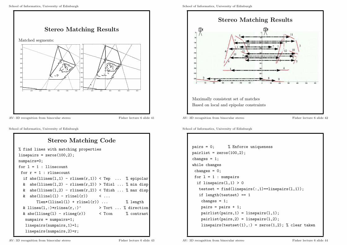
Finding line segments
Some random data crossings
Want to find approximate observed start and end of true segment
1. Project points {~xi} onto ideal line thru point ~p with direction
~a: λi = (~xi − ~p) · ~a. Projected point is ~p + λi~a
p
ax
λ
2. Remove points not having 43 neighbor points within 45 pixels
distance
3. Endpoints are given by smallest and largest remaining λi.
AV: 3D recognition from binocular stereo Fisher lecture 6 slide 24
School of Informatics, University of Edinburgh
Found line segments
AV: 3D recognition from binocular stereo Fisher lecture 6 slide 25
School of Informatics, University of Edinburgh
Stereo Overview
AV: 3D recognition from binocular stereo Fisher lecture 6 slide 26
School of Informatics, University of Edinburgh
Line Segment Description
Given line segment endpoints ~b and ~c with direction ~a = (u, v):
L
R
D
Dn
x
b
c
a
d
λ
Orientation: compute perpendicular ~n = (−v, u)
Position: estimate midpoint ~m = (~b + ~c)/2
Shape: estimate length || ~b − ~c ||
AV: 3D recognition from binocular stereo Fisher lecture 6 slide 27
School of Informatics, University of Edinburgh
Estimate edge contrast of pixels within D of line in regions L & R:
For any pixel ~x
If 0 ≤ (~x −~b) · ~a ≤|| ~b − ~c ||
If 0 < (~x −~b) · ~n ≤ D, put ~x in L
If −D ≤ (~x −~b) · ~n < 0, put ~x in R
Estimate contrast g = (average brightness of pixels in L)
- (average brightness of pixels in R)
Description is direction ~a, midpoint ~m, length || ~b − ~c || and
contrast g.
AV: 3D recognition from binocular stereo Fisher lecture 6 slide 28

School of Informatics, University of Edinburgh
Corresponding Line Properties
Edges L dir R dir L len R len
L1:R4 (0.00,-1.00) (0.00,-1.00) 137 125
L5:R11 (0.45,0.89) (0.38,0.93) 90 119
L6:R7 (0.96,-0.28) (0.96,-0.29) 291 251
L7:R2 (0.95,0.32) (1.00,0.00) 93 140
L8:R5 (0.70,-0.71) (0.86,-0.50) 49 61
L10:R12 (0.81,-0.59) (0.86,-0.52) 87 82
L11:R10 (-0.33,-0.94) (-0.29,-0.96) 72 101
L12:R3 (0.89,0.45) (0.96,0.28) 129 115
AV: 3D recognition from binocular stereo Fisher lecture 6 slide 29
School of Informatics, University of Edinburgh
Edges L mid R mid L con R con
L1:R4 (370,369) (364,242) -91 -37
L5:R11 (55,477) (40,309) 28 18
L6:R7 (158,355) (181,194) 44 55
L7:R2 (74,416) (90,246) -117 -44
L8:R5 (250,567) (278,371) -66 -31
L10:R12 (208,402) (205,221) 38 55
L11:R10 (199,536) (195,358) 141 113
L12:R3 (140,554) (132,400) 47 23
AV: 3D recognition from binocular stereo Fisher lecture 6 slide 30
School of Informatics, University of Edinburgh
Binocular Stereo
Goal: build 3D scene description (eg. depth) given two 2D image
descriptions
Useful for: obstacle avoidance, grasping, object location
Key principle: triangulation
D
α β
LEFTSENSOR
RIGHTSENSOR
AV: 3D recognition from binocular stereo Fisher lecture 6 slide 31
School of Informatics, University of Edinburgh
Image Features
What to match?
Edge fragments from edge detector. Usually many.
Larger structures, like lines (RANSAC, vertical for mobile robots)
Larger easier to match but harder to get and less dependable
Human visual system thought to work at edge fragment level
AV: 3D recognition from binocular stereo Fisher lecture 6 slide 32

School of Informatics, University of Edinburgh
Stereo Correspondence Problem
Which feature in left image matches a given feature in the right?LEFT RIGHT
WHICH?{Different pairings give different depth results
Often considered the key problem of stereo
AV: 3D recognition from binocular stereo Fisher lecture 6 slide 33
School of Informatics, University of Edinburgh
Constraining Matches: Edge Direction
:
OK BAD BADMatch features with nearly same orientation
AV: 3D recognition from binocular stereo Fisher lecture 6 slide 34
School of Informatics, University of Edinburgh
Constraining Matches: Edge Contrast
:
OK BAD BADMatch features with nearly same contrast across edge
AV: 3D recognition from binocular stereo Fisher lecture 6 slide 35
School of Informatics, University of Edinburgh
Constraining Matches: Feature Shape
:
OK BAD BADMatch features with nearly same length
AV: 3D recognition from binocular stereo Fisher lecture 6 slide 36
School of Informatics, University of Edinburgh
Constraining Matches: Uniqueness and
Smoothness
Smoothness: match features giving nearly same depth as neighbors
Uniqueness: a feature in one image can match from the other
image:
0 - occlusion
1 - normal case
2+ - transparencies, wires, vines, etc from coincidental alignments
AV: 3D recognition from binocular stereo Fisher lecture 6 slide 37
School of Informatics, University of Edinburgh
Midlecture Problem
Which stereo correspondence constraintwould you use to reject these matches?
:
AV: 3D recognition from binocular stereo Fisher lecture 6 slide 38
School of Informatics, University of Edinburgh
Constraining Matches: Epipolar
Geometry
Feature ~pl in left image lies on a ray ~r thru space.
~r projects to an epipolar line e in the right image, along which the
matching image feature must lie.
lp
+Z
+Y
+X
e
r
p r
p
AV: 3D recognition from binocular stereo Fisher lecture 6 slide 39
School of Informatics, University of Edinburgh
If images are ‘rectified’, then the epipolar line is an image row.
Reduces 2D search to 1D search
lp
+Z
+Y
+X
e
r
p r
p
Images are linked by the Fundamental matrix F
Matched points satisfy ~p′lF~pr = 0
(Points are in homogeneous coordinates, F is 3 × 3)
AV: 3D recognition from binocular stereo Fisher lecture 6 slide 40
School of Informatics, University of Edinburgh
Stereo Matching Results
Matched segments:
0 100 200 300 400 500 600
0
50
100
150
200
250
300
350
400
450
0 100 200 300 400 500 600
0
50
100
150
200
250
300
350
400
450
AV: 3D recognition from binocular stereo Fisher lecture 6 slide 41
School of Informatics, University of Edinburgh
Stereo Matching Results
Maximally consistent set of matches
Based on local and epipolar constraints
AV: 3D recognition from binocular stereo Fisher lecture 6 slide 42
School of Informatics, University of Edinburgh
Stereo Matching Code
% find lines with matching properties
linepairs = zeros(100,2);
numpairs=0;
for l = 1 : llinecount
for r = 1 : rlinecount
if abs(llinem(l,1) - rlinem(r,1)) < Tep ... % epipolar
& abs(llinem(l,2) - rlinem(r,2)) > Tdisl ... % min disp
& abs(llinem(l,2) - rlinem(r,2)) < Tdish ... % max disp
& abs(llinel(l) - rlinel(r)) < ...
Tlen*(llinel(l) + rlinel(r)) ... % length
& llinea(l,:)*rlinea(r,:)’ > Tort ... % direction
& abs(llineg(l) - rlineg(r)) < Tcon % contrast
numpairs = numpairs+1;
linepairs(numpairs,1)=l;
linepairs(numpairs,2)=r;
AV: 3D recognition from binocular stereo Fisher lecture 6 slide 43
School of Informatics, University of Edinburgh
pairs = 0; % Enforce uniqueness
pairlist = zeros(100,2);
changes = 1;
while changes
changes = 0;
for l = 1 : numpairs
if linepairs(l,1) > 0
testset = find(linepairs(:,1)==linepairs(l,1));
if length(testset) == 1
changes = 1;
pairs = pairs + 1;
pairlist(pairs,1) = linepairs(l,1);
pairlist(pairs,2) = linepairs(l,2);
linepairs(testset(1),:) = zeros(1,2); % clear taken
AV: 3D recognition from binocular stereo Fisher lecture 6 slide 44
School of Informatics, University of Edinburgh
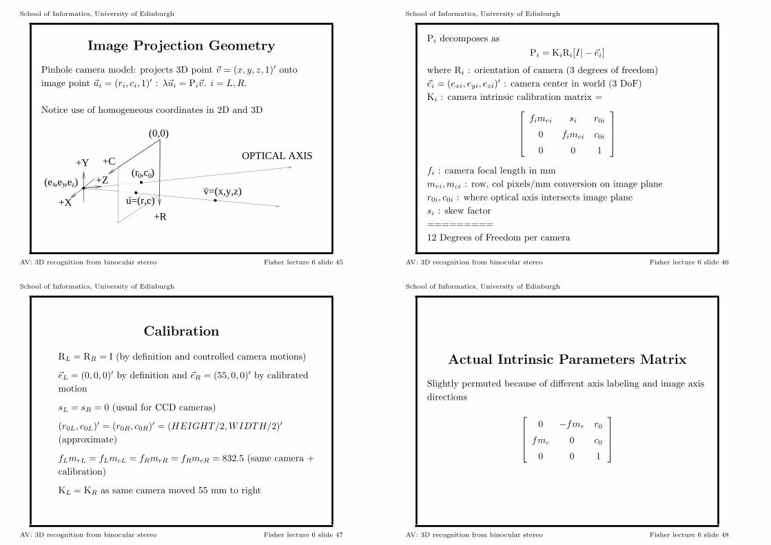
Image Projection Geometry
Pinhole camera model: projects 3D point ~v = (x, y, z, 1)′ onto
image point ~ui = (ri, ci, 1)′ : λ~ui = Pi~v. i = L, R.
Notice use of homogeneous coordinates in 2D and 3D
(r ,c )0 0
v=(x,y,z)+X
+Y
+Z
+C
+R
(0,0)
OPTICAL AXIS
zyx(e ,e ,e )
u=(r,c)
AV: 3D recognition from binocular stereo Fisher lecture 6 slide 45
School of Informatics, University of Edinburgh
Pi decomposes as
Pi = KiRi[I| − ~ei]
where Ri : orientation of camera (3 degrees of freedom)
~ei = (exi, eyi, ezi)′ : camera center in world (3 DoF)
Ki : camera intrinsic calibration matrix =
fimri si r0i
0 fimci c0i
0 0 1
fi : camera focal length in mm
mri, mci : row, col pixels/mm conversion on image plane
r0i, c0i : where optical axis intersects image plane
si : skew factor
=========
12 Degrees of Freedom per camera
AV: 3D recognition from binocular stereo Fisher lecture 6 slide 46
School of Informatics, University of Edinburgh
Calibration
RL = RR = I (by definition and controlled camera motions)
~eL = (0, 0, 0)′ by definition and ~eR = (55, 0, 0)′ by calibrated
motion
sL = sR = 0 (usual for CCD cameras)
(r0L, c0L)′ = (r0R, c0R)′ = (HEIGHT/2, WIDTH/2)′
(approximate)
fLmrL = fLmcL = fRmrR = fRmcR = 832.5 (same camera +
calibration)
KL = KR as same camera moved 55 mm to right
AV: 3D recognition from binocular stereo Fisher lecture 6 slide 47
School of Informatics, University of Edinburgh
Actual Intrinsic Parameters Matrix
Slightly permuted because of different axis labeling and image axis
directions
0 −fmr r0
fmc 0 c0
0 0 1
AV: 3D recognition from binocular stereo Fisher lecture 6 slide 48
School of Informatics, University of Edinburgh
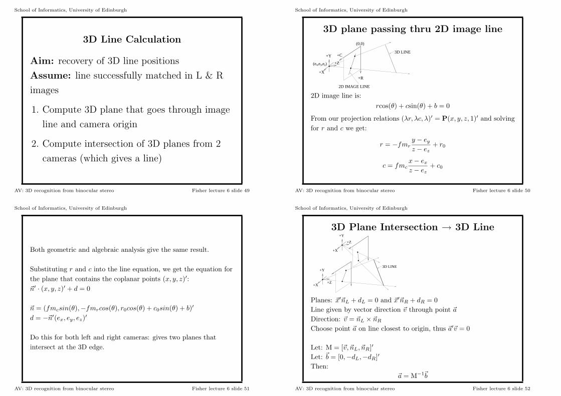
3D Line Calculation
Aim: recovery of 3D line positions
Assume: line successfully matched in L & R
images
1. Compute 3D plane that goes through image
line and camera origin
2. Compute intersection of 3D planes from 2
cameras (which gives a line)
AV: 3D recognition from binocular stereo Fisher lecture 6 slide 49
School of Informatics, University of Edinburgh
3D plane passing thru 2D image line
+X
+Y
+Z
+C
+R
(0,0)
3D LINE
2D IMAGE LINE
(e ,e ,e )zyx
2D image line is:
rcos(θ) + csin(θ) + b = 0
From our projection relations (λr, λc, λ)′ = P(x, y, z, 1)′ and solving
for r and c we get:
r = −fmr
y − ey
z − ez
+ r0
c = fmc
x − ex
z − ez
+ c0
AV: 3D recognition from binocular stereo Fisher lecture 6 slide 50
School of Informatics, University of Edinburgh
Both geometric and algebraic analysis give the same result.
Substituting r and c into the line equation, we get the equation for
the plane that contains the coplanar points (x, y, z)′:
~n′ · (x, y, z)′ + d = 0
~n = (fmcsin(θ),−fmrcos(θ), r0cos(θ) + c0sin(θ) + b)′
d = −~n′(ex, ey, ez)′
Do this for both left and right cameras: gives two planes that
intersect at the 3D edge.
AV: 3D recognition from binocular stereo Fisher lecture 6 slide 51
School of Informatics, University of Edinburgh
3D Plane Intersection → 3D Line
3D LINE
+X
+Y
+Z
+X
+Y
+Z
Planes: ~x′~nL + dL = 0 and ~x′~nR + dR = 0
Line given by vector direction ~v through point ~a
Direction: ~v = ~nL × ~nR
Choose point ~a on line closest to origin, thus ~a′~v = 0
Let: M = [~v, ~nL, ~nR]′
Let: ~b = [0,−dL,−dR]′
Then:
~a = M−1~b
AV: 3D recognition from binocular stereo Fisher lecture 6 slide 52
School of Informatics, University of Edinburgh
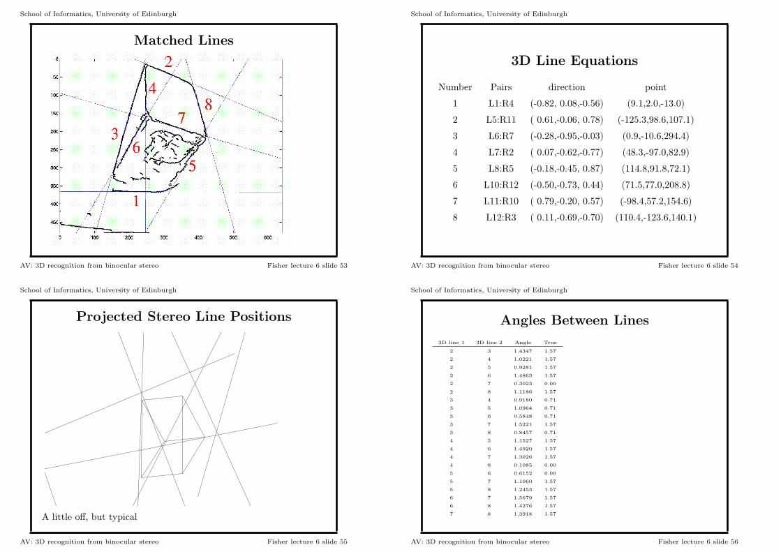
Matched Lines
AV: 3D recognition from binocular stereo Fisher lecture 6 slide 53
School of Informatics, University of Edinburgh
3D Line Equations
Number Pairs direction point
1 L1:R4 (-0.82, 0.08,-0.56) (9.1,2.0,-13.0)
2 L5:R11 ( 0.61,-0.06, 0.78) (-125.3,98.6,107.1)
3 L6:R7 (-0.28,-0.95,-0.03) (0.9,-10.6,294.4)
4 L7:R2 ( 0.07,-0.62,-0.77) (48.3,-97.0,82.9)
5 L8:R5 (-0.18,-0.45, 0.87) (114.8,91.8,72.1)
6 L10:R12 (-0.50,-0.73, 0.44) (71.5,77.0,208.8)
7 L11:R10 ( 0.79,-0.20, 0.57) (-98.4,57.2,154.6)
8 L12:R3 ( 0.11,-0.69,-0.70) (110.4,-123.6,140.1)
AV: 3D recognition from binocular stereo Fisher lecture 6 slide 54
School of Informatics, University of Edinburgh
Projected Stereo Line Positions
A little off, but typical
AV: 3D recognition from binocular stereo Fisher lecture 6 slide 55
School of Informatics, University of Edinburgh
Angles Between Lines
3D line 1 3D line 2 Angle True
2 3 1.4347 1.57
2 4 1.0221 1.57
2 5 0.9281 1.57
2 6 1.4863 1.57
2 7 0.3023 0.00
2 8 1.1186 1.57
3 4 0.9180 0.71
3 5 1.0964 0.71
3 6 0.5848 0.71
3 7 1.5221 1.57
3 8 0.8457 0.71
4 5 1.1527 1.57
4 6 1.4920 1.57
4 7 1.3026 1.57
4 8 0.1085 0.00
5 6 0.6152 0.00
5 7 1.1060 1.57
5 8 1.2453 1.57
6 7 1.5679 1.57
6 8 1.4276 1.57
7 8 1.3918 1.57
AV: 3D recognition from binocular stereo Fisher lecture 6 slide 56
School of Informatics, University of Edinburgh
3D Edge Based Recognition Pipeline
AV: 3D recognition from binocular stereo Fisher lecture 6 slide 57
School of Informatics, University of Edinburgh
3D Edge Based Recognition
Match 3D data edges to 3D wireframe model edges
M4
M6
M3
M7
M9M5M2M1
M8
+Z
(0,0,46)
(0,67,0)
+X +Y
(67,0,0)
(0,0,0)
Model =
(0,0,0)-(67,0,0)
(0,0,0)-(0,67,0)
(0,0,0)-(0,0,46)
(67,0,0)-(67,0,46)
(0,67,0)-(0,67,46)
(0,0,46)-(67,0,46)
(0,0,46)-(0,67,46)
(67,0,0)-(0,67,0)
(67,0,46)-(0,67,46)
AV: 3D recognition from binocular stereo Fisher lecture 6 slide 58
School of Informatics, University of Edinburgh
3D Model Matching
Use Interpretation Tree algorithm: matchedges, Limit = 5
Unary test: similar length | lm − ld |< τl(lm + ld)
Binary test: similar angle between pairs:| θm − θd |< τa
AV: 3D recognition from binocular stereo Fisher lecture 6 slide 59
School of Informatics, University of Edinburgh
Matching Performance
144 interpretation tree matches thru to pose estimation and
verification
Two valid solutions found (symmetric model rotated 180 degrees)
Data Model 1 Model 2
Segment Segment Segment
3 M8 M9
4 M2 M6
6 M1 M7
7 M3 M3
8 M7 M1
AV: 3D recognition from binocular stereo Fisher lecture 6 slide 60
School of Informatics, University of Edinburgh
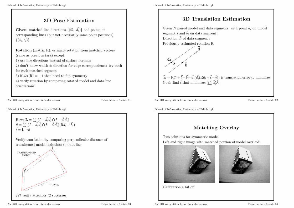
3D Pose Estimation
Given: matched line directions {(~mi, ~di)} and points on
corresponding lines (but not necessarily same point positions)
{(~ai,~bi)}
Rotation (matrix R): estimate rotation from matched vectors
(same as previous task) except:
1) use line directions instead of surface normals
2) don’t know which ± direction for edge correspondence: try both
for each matched segment
3) if det(R) = −1 then need to flip symmetry
4) verify rotation by comparing rotated model and data line
orientations
AV: 3D recognition from binocular stereo Fisher lecture 6 slide 61
School of Informatics, University of Edinburgh
3D Translation Estimation
Given N paired model and data segments, with point ~ai on model
segment i and ~bi on data segment i
Direction ~di of data segment i
Previously estimated rotation R
b
a
d
Rλ
~λi = R~ai +~t−~b− ~di(~d′
i(R~ai +~t−~b)) is translation error to minimize
Goal: find ~t that minimizes∑
i~λ′
i~λi
AV: 3D recognition from binocular stereo Fisher lecture 6 slide 62
School of Informatics, University of Edinburgh
How: L =∑
i(I − ~di~d′i)
′(I − ~di~d′i)
~n =∑
i(I − ~di~d′i)
′(I − ~di~d′i)(R~ai −~bi)
~t = L−1~n
Verify translation by comparing perpendicular distance of
transformed model endpoints to data line
TRANSFORMEDMODEL
λ
λ
DATA
287 verify attempts (2 successes)
AV: 3D recognition from binocular stereo Fisher lecture 6 slide 63
School of Informatics, University of Edinburgh
Matching Overlay
Two solutions for symmetric model
Left and right image with matched portion of model overlaid:
Calibration a bit off
AV: 3D recognition from binocular stereo Fisher lecture 6 slide 64
School of Informatics, University of Edinburgh
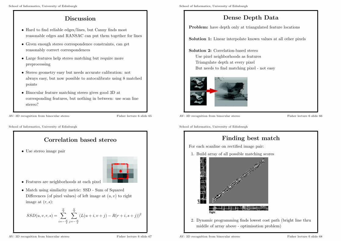
Discussion
• Hard to find reliable edges/lines, but Canny finds most
reasonable edges and RANSAC can put them together for lines
• Given enough stereo correspondence constraints, can get
reasonably correct correspondences
• Large features help stereo matching but require more
preprocessing
• Stereo geometry easy but needs accurate calibration: not
always easy, but now possible to autocalibrate using 8 matched
points
• Binocular feature matching stereo gives good 3D at
corresponding features, but nothing in between: use scan line
stereo?
AV: 3D recognition from binocular stereo Fisher lecture 6 slide 65
School of Informatics, University of Edinburgh
Dense Depth Data
Problem: have depth only at triangulated feature locations
Solution 1: Linear interpolate known values at all other pixels
Solution 2: Correlation-based stereo
Use pixel neighborhoods as features
Triangulate depth at every pixel
But needs to find matching pixel - not easy
AV: 3D recognition from binocular stereo Fisher lecture 6 slide 66
School of Informatics, University of Edinburgh
Correlation based stereo
• Use stereo image pair
• Features are neighborhoods at each pixel
• Match using similarity metric: SSD - Sum of Squared
Differences (of pixel values) of left image at (u, v) to right
image at (r, s):
SSD(u, v, r, s) =
N
2∑
i=−N
2
N
2∑
j=−N
2
(L(u + i, v + j) − R(r + i, s + j))2
AV: 3D recognition from binocular stereo Fisher lecture 6 slide 67
School of Informatics, University of Edinburgh
Finding best match
For each scanline on rectified image pair:
1. Build array of all possible matching scores
2. Dynamic programming finds lowest cost path (bright line thru
middle of array above - optimisation problem)
AV: 3D recognition from binocular stereo Fisher lecture 6 slide 68
School of Informatics, University of Edinburgh
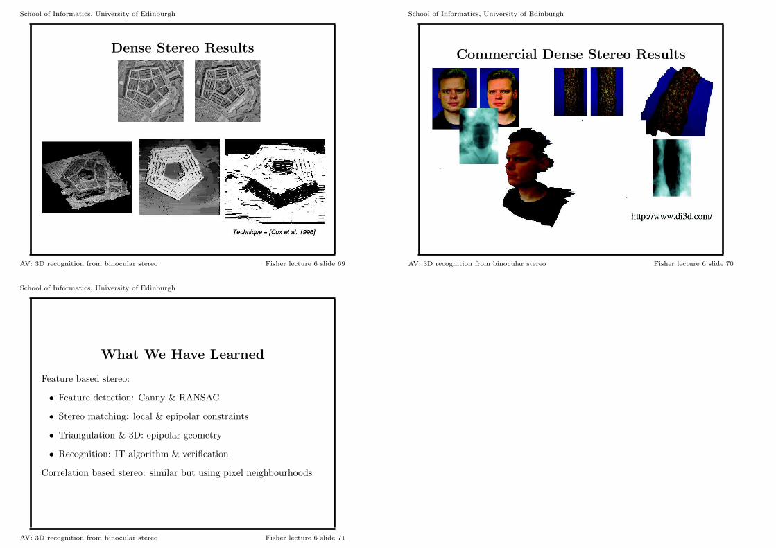
Dense Stereo Results
AV: 3D recognition from binocular stereo Fisher lecture 6 slide 69
School of Informatics, University of Edinburgh
Commercial Dense Stereo Results
AV: 3D recognition from binocular stereo Fisher lecture 6 slide 70
School of Informatics, University of Edinburgh
What We Have Learned
Feature based stereo:
• Feature detection: Canny & RANSAC
• Stereo matching: local & epipolar constraints
• Triangulation & 3D: epipolar geometry
• Recognition: IT algorithm & verification
Correlation based stereo: similar but using pixel neighbourhoods
AV: 3D recognition from binocular stereo Fisher lecture 6 slide 71