BING3D: Fast Spatio-Temporal Proposals for Action Localization

Ella GatiUniversity of Amsterdam

John G. M. SchavemakerTNO

Jan C. van GemertDelft University of Technology

Abstract

The goal of this work is realistic action localization invideo with the aid of spatio-temporal proposals. Currentproposal generation methods are computationally demand-ing and are not practical for large-scale datasets. The maincontribution of this work is a novel and fast alternative.Our method uses spatio-temporal gradient computations, ageneralization of BING to the temporal domainleading toBING3D. The method is orders of magnitude faster thancurrent methods and performs on par or above the localiza-tion accuracy of current proposals on the UCF sports andMSR-II datasets. Furthermore, due to our efficiency, we arethe first to report action localization results on the largeand challenging UCF 101 dataset. Another contributionof this work is our Apenheul case study, where we createdand tested our proposals performance on a novel and chal-lenging dataset. The Apenheul dataset is large-scale, as itcontains full high definition videos, featuring gorillas in anatural environment, with uncontrolled background, light-ing conditions and quality.

1. Introduction

Action localization (1) deals with unraveling when,where and what happens in a video. In this work we pro-pose a method for action localization using spatio-temporalproposals, which is fast and achieves state-of-the-art results.The naive approach to action localization is using a slidingsub-volume, which is the 3D extension of the sliding win-dow approach for static images. While effective for staticimages [15], when dealing with videos sliding window ap-proaches become computationally intractable even for mod-est sized videos.

More recent methods for action localization [10, 20, 30]are proposals based. This is inspired by successful object-proposals methods in static images [1, 4, 19, 29]. Proposalbased methods first reduce the search space to a small setof spatio-temporal tubes, with high likelihood to contain anaction. Compared to sliding-subvolume approaches, suchas [12, 24, 26], proposals for action localization are moreefficient and allow using bigger datasets. Another advan-

Golf swing

Golf swing

Figure 1. Action localization aims to find where, when and whataction is taking place in a video. The red tubelet is the groundtruth, the blue cuboid is our best proposal. The action label indi-cates what action is taking place.

tage of proposal based methods is that the small numberof proposals that has to be classified makes it possible touse more computationally expensive features and more ad-vanced classifiers, that would be impractical otherwise, toachieve state-of-the-art localization accuracy.

Current action proposal algorithms are based on densetrajectories [30] or use video segmentation [10, 20] to gen-erate the action proposals. Segmentation is computationalexpensive, and takes several minutes for a modest video of720x400 video of 55 frames [20, 35] and can take days fora realistic full HD video. The computational demands ofsegmentation based action proposals are not practical forlarge-scale video processing. This is the main motivationfor creating a fast large-scale action localization method.

In this work, we present BING3D, a generalization ofBING [4] from image to video for high speed 3D propos-als, in which we use spatio-temporal video gradients insteadof video segmentation. We chose BING because of its im-pressive speed and small number of quality object propos-als. The strength of BING’s efficiency lies in simple gra-dient features and an approximation method for fast pro-posal selection. We generalize to the temporal domain byadding temporal features, and a spatio-temporal approxima-tion method leading to BING3D.

1

BING3D is orders of magnitude faster than current meth-ods and performs on par or above the localization accuracyof current proposals on benchmark datasets.

section 2 gives a short review of the related research inthe field. The method is described and explained in section3. We present the experimental setup, as well as experi-ments results and analysis in section 4. Finally we concludeour work in section 5.

2. Related WorkSeveral action localization methods apply an action clas-

sifier directly on the video. Examples include sliding 3Dsubvolume methods like spatio-temporal template match-ing [24], a 3D boosting cascade [12] and spatio-temporaldeformable 3D parts [26]. Other methods maximize atemporal classification path of 2D boxes through staticframes [27, 28] or search for the optimal classification resultwith a branch and bound scheme [36]. The benefit is thatthese methods do not require an intermediate representationand directly apply a classifier to densely sampled parts ofthe video. The disadvantage of such methods, however, isthat they have to perform the same dense sampling for eachindividual action class separately. Due to the computationalcomplexity of the sampling, this is impractical for largernumbers of action classes. Instead, we use spatio-temporalproposals to first generate a small set of bounding-box tubesthat are likely to contain any type of action.

Current spatio-temporal proposals are inspired by 2Dobject proposals in static images. A version of object-ness [1] is extened to video [2], selective search [29] ledto tubelets from motion [10] and randomized Prim [19]was generalized to a spatio-temporal variant [20]. Several2D object proposal methods and their 3D generalizationsare based on a super-pixel segmentation pre-processingstep [1, 2, 10, 14, 19, 20, 29] which we argue is compu-tationally too demanding for large scale video processing.Other 2D proposal methods such as edge boxes [38] useedge-detection and BING [4] uses gradient computation aspre-processing steps. Since gradients are the fastest to com-pute we propose a 3D extension of BING for large-scalespatio-temporal action proposals. To avoid the expensivepre-processing step altogether, we also propose a method ofgenerating proposals without any pre-processing. This sec-ond method generates proposals from the local features asrequired later on by the action classifier.

Local features provide a solid base for action recognitionand action localization. Points are sampled at salient spatio-temporal locations [6, 17], densely [25, 34] or along densetrajectories [31, 33]. The points are represented by pow-erful local descriptors [18, 13, 5] that are robust to modestchanges in motion and in appearance. Robustness to cameramotion is either directly modeled from the video [9, 33] ordealt with at the feature level by the MBH descriptor [5, 31].

After aggregating local descriptors in a global video repre-sentation such as VLAD [9] or Fisher [21, 22, 33] they areinput to a classifier like SVM. Due to the excellent perfor-mance of dense trajectory features [31, 33] in action local-ization [10], we adopt them as our feature representationthroughout this paper.

3. Method

The generation of action proposals is done usingBING3D, our extension of the BING [4] algorithm fromstatic images to videos. BING stands for ’BInariazed Nor-malized Gradient’, as it is based on image gradient as itsbasic features. Image derivatives, as well as their three-dimensional extension for videos, are simple features thatcan be computed efficiently. It has been shown that ob-jects tend to have well-defined object boundaries [4], thatare captured correctly by the spatial derivatives magnitude.Adding the temporal derivative to the gradient is imperativeto capture the temporal extent of an action.

3.1. NG3D

We use normalized video gradients (referred to asNG3D) as the base to our features. The gradient of videov is defined by the partial derivatives of each dimension|∇v| = |(vx, vy, vz)T |, where vx, vy, vz are the partialderivative of the x, y, z axes respectively. The partial deriva-tives are efficiently computed by convolving the video vwith a 1D mask [-1 0 1], which is an approximation ofthe Gaussian derivative, in each dimension separately. Foreach pixel the gradient magnitude is computed and thenclipped at 255 to fit the value in a byte, as min(|vx| +|vy| + |vz|, 255). The final feature vector is the L1 nor-malized, concatenated gradient magnitudes of a pixel block.The shape of the pixel block is 8x8 spatially, so it fits in asingle int64 variable, which allow for easy use of bitwiseoperations, and we vary the temporal depth of the featureDresulting in a 8× 8×D block. In section 4 we evaluate theperformance when varying the temporal depth D.

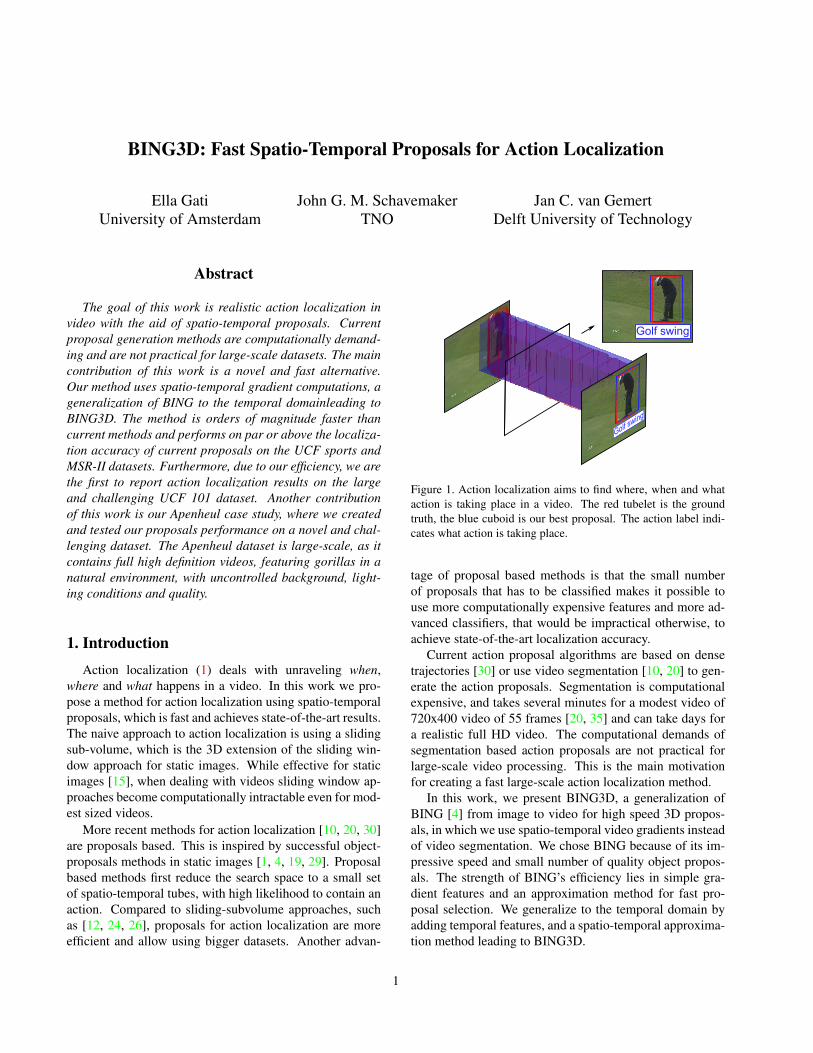
Figure 2 illustrates the NG3D features. The top rowis showing a sequence of random frames from one of thetraining videos. The red boxes are random boxes of non-action, while the green boxes cover a Running action. Thebottom boxes illustrate the spatio-temporal NG3D featuresof the boxes drawn on top. The action is described withD = 4 temporal layers on NG3D feature, while randomblocks from the same video do not display a similar patternillustrating that the NG3D feature can be used for discrimi-nating actions from non-actions.

In order to generate diverse proposals in terms of width,height and length, we first resize our videos to a set of pre-defined scales (1/2, 1/4, 1/8, 1/16, 1/32), using trilinear in-terpolation.

Figure 2. Visualization of 3D Normalized Gradients (NG3D). Top:The red boxes are on non-action parts in the video, the green boxcovers a Running action. Bottom: visualisation of the spatio-temporal NG3D features in the red and green boxes from the topin 8 × 8 spatial resolution and D = 4 temporal frames. The ac-tion is clearly described with NG3D feature, while random blocksfrom the same video do not display a similar pattern illustratingthat the NG3D feature can be used for discriminating actions fromnon-actions.

3.2. BING3D

To compute BING3D, we learn a classifier model, com-pute its approximation and then binarize the NG3D featuresto what we call BING3D. The computed features and ap-proximated model are used to compute proposal scores.

Learning a classifier model The positive samples in thetrain set are approximations of the ground truth tracks. Eachtrack is enlarged to a cuboid and then resized with differentscales. Cuboids that overlap more than a threshold (0.25)with the ground truth cuboid are used as positive samples.The negative samples are random cusboids that do ot over-lap with any gt track. We use linear SVM to learn modelw.

Approximate model Efficient proposal classification isachieved by approximating the SVM model w in a binaryembedding [4, 8] which allows fast bitwise operations inthe evaluation. The learned model w ∈ R8×8×D is approx-imated by a set of binary basis vectors a ∈ {−1, 1}8×8 andtheir coefficients β ∈ R. The approximation becomes

w ≈D∑i=1

Nw∑j=1

βijaij . (1)

In section 4 we evaluate the quality of the approximationwith different number of components Nw. Pseudo code forcomputing the binary embedding is given in algorithm 1.

Generating BING3D features In addition to the approx-imation of the model, we also approximate the normed gra-dient values using the top Ng binary bits of the BYTE val-ues. Thus, each dimension of the NG3D feature gl can be

Algorithm 1 Binary approximation of wInput: w, Nw, DOutput: {{βij}Nw

j=1}Di=1, {{aij}Nwj=1}Di=1

for i = 1 to D doε = wi

for j = 1 to Nw doaij = sign(ε)βij = 〈aij , ε〉/||aij ||2ε← ε− βijaij

end forend for

approximated by Ng binarized normed gradient features as:

gl =

Ng∑k=1

28−kbk,l (2)

where l = (i, x, y, z) is the scale and location of the fea-ture. The 8 × 8 ×D patches of approximated gradient arethe BING3D features. As with the approximation of w, weapproximate each temporal slice independently. We use thefast algorithm proposed in [4], and presented in algorithm2 to compute the 8 × 8 feature for each of the D temporalslices. Thanks to the cumulative relation between adjacentBING3D features and their last rows, we can avoid loop-ing over the 8 × 8 region, by using BITWISE SHIFT andBITWISE OR operations.

Algorithm 2 BING [4] algorithm to compute BING fea-tures for W ×H positionsInput: binary normed gradient map bW×HOutput: BING feature matrix bW×H

Initialize: bW×H = 0, rW×H = 0for each position (x, y) in scan-line order dorx,y = (rx−1,y � 1) | bx,ybx,y = (bx,y−1 � 8) | rx,y

end for

Proposals Generation The proposal generation processinvolves computing an approximated classifier score (or’proposal score’) sl for each scale and location in the videoand then choosing only the top scored proposals.

The approximated classifier score is defined as

sl = 〈w, gl〉 (3)

and can be efficiently tested using:

sl ≈D∑i=1

Nw∑j=1

βij

Ng∑k=1

28−k(2〈a+ij ,bk,l〉 − |bk,l|) (4)

We use non-maximum suppression to reduce the numberof proposals according to their proposal score.

3.3. Action Localization

We use the state-of-art descriptors computed along im-proved dense trajectory [33]. To represent a proposal, weaggregate all the visual words corresponding to the trajec-tories that fall inside of it. For training, we use a one-vs-restlinear SVM classifier.

4. Experiments4.1. Datasets

We evaluate on three diverse datasets for action local-ization: UCF Sports, UCF 101 and MSR-II. UCF Sportsconsists of 150 videos extracted from sports broadcasts ofvarying resolution; it is trimmed to contain a single actionin all frames. UCF101 is collected from YouTube and has101 action categories where 24 of them contain localizationannotations, corresponding to 3,204 videos. All UCF101videos contain exactly one action1, most of them (74.6%)are trimmed to fit the action. In contrast, the MSR-II Ac-tion dataset consists of 203 actions in 54 videos where eachvideo has multiple actions of three classes. The actionsare performed in a crowded environment with ample back-ground movement. The MSR-II videos are relatively long,on average 763 frames, and the videos are untrimmed.

4.2. Experimental Setup

For all experiments in this section we use a train-test splitand state results obtained on the test set. For UCF Sportsand UCF 101 we use the standard split, and for MSR-IIa random split of 50% train and 50% test videos. SinceUCF-sports and UCF 101 are trimmed, BING3D outputsfull length proposals for them. Both in BING3D and in thelocalization training, we set the positive samples thresholdto 0.25 in all experiments. We used liblinear [7] everywhereSVM is used, and the SVM parameter is set using crossvalidation. We used default parameters in the extraction ofthe improved dense trajectories. For the Fisher encoding,we always reduced descriptors’ dimensionality to half, assuggested in [32].

In the experiments and evaluation of the algorithm weused three benchmark action localization datasets, namelyUCF Sports, UCF 101 and MSR-II

We used different methods to quantify the performanceof our algorithms. For the proposals quality evaluation weused the ABO, MABO and Best Overlap recall measures,as explained in more details next. The action localization isevaluated using average precision and AUC.

The proposal quality of a proposal P with a groundtruth tube G is evaluated with spatio-temporal tube over-lap measured as the average ”intersection-over-union” scorefor 2D boxes for all frames where there is either a ground

1We used the first annotated “person” in the XML file.

truth box or a proposal box. More formally, for a videoV of F frames, a tube of bounding boxes is given by(B1, B2, ...BF ), where Bf = ∅, if there is no action i inframe f , φ is the set of frames where at least one of Gf , Pfis not empty. The localization score between G and P isL(G,P ) = 1

|φ|∑f∈φ

Gf∩Pf

Gf∪Pf.

The Average Best Overlap (ABO) score is computed byaveraging the localization score of the best proposal foreach ground truth action. The Mean Average Best Over-lap (MABO) is the mean of the per class ABO score. Therecall is the percentage of ground truth actions with bestoverlap score over a threshold. It is is worth mentioningthat although other papers often use 0.2 as the threshold, wechose to use stricter criteria, thus unless stated otherwise wereport recall with a 0.5 threshold.

The localization performance is measured in means ofaverage precision (AP) and mean average precision (mAP).To compute average precision, the proposals are sorted ac-cording to their classification score. A proposal is consid-ered relevant if its label is predicted correctly and its over-lap score with the ground truth tubelet is over a threshold.We present plots of AP and mAP scores for different over-lap thresholds. For comparability with previous works , wealso provide AUC plot, computed as in [16].

4.3. Experiments

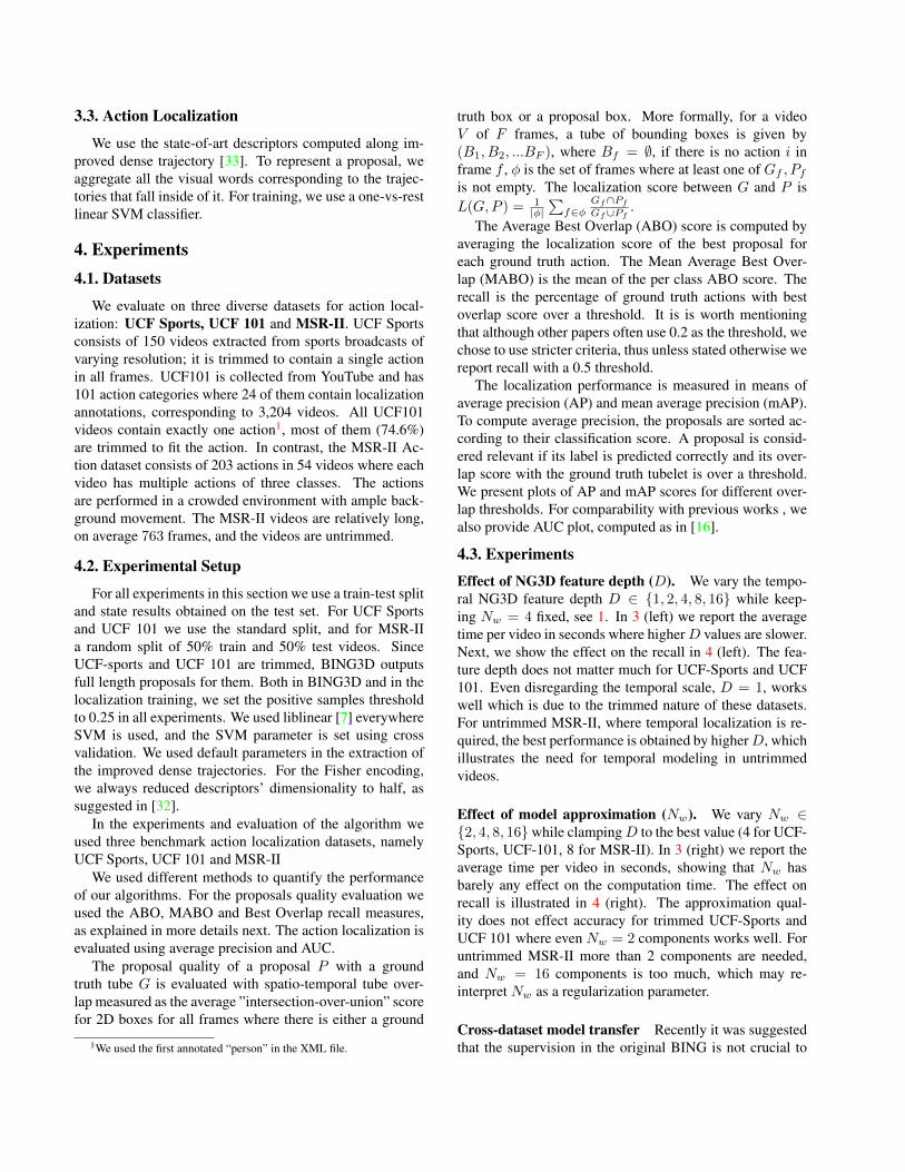
Effect of NG3D feature depth (D). We vary the tempo-ral NG3D feature depth D ∈ {1, 2, 4, 8, 16} while keep-ing Nw = 4 fixed, see 1. In 3 (left) we report the averagetime per video in seconds where higherD values are slower.Next, we show the effect on the recall in 4 (left). The fea-ture depth does not matter much for UCF-Sports and UCF101. Even disregarding the temporal scale, D = 1, workswell which is due to the trimmed nature of these datasets.For untrimmed MSR-II, where temporal localization is re-quired, the best performance is obtained by higherD, whichillustrates the need for temporal modeling in untrimmedvideos.

Effect of model approximation (Nw). We vary Nw ∈{2, 4, 8, 16}while clampingD to the best value (4 for UCF-Sports, UCF-101, 8 for MSR-II). In 3 (right) we report theaverage time per video in seconds, showing that Nw hasbarely any effect on the computation time. The effect onrecall is illustrated in 4 (right). The approximation qual-ity does not effect accuracy for trimmed UCF-Sports andUCF 101 where even Nw = 2 components works well. Foruntrimmed MSR-II more than 2 components are needed,and Nw = 16 components is too much, which may re-interpret Nw as a regularization parameter.

Cross-dataset model transfer Recently it was suggestedthat the supervision in the original BING is not crucial to

UCF Sports UCF 101 MSR−II0123456789

101112131415161718

Tim

e (s

econ

ds)

Effect of NG3D feature depth on time

D=1D=2D=4D=8D=16

UCF Sports UCF 101 MSR−II0

1

2

3

4

5

Tim

e (s

econ

ds)

Effect of number of components on time

#Comp=2#Comp=4#Comp=8#Comp=16

Effect of D Effect of NwFigure 3. Evaluating BING3D parameters D (left) and Nw (right)on computation time (s). The feature depth has a strong impact onthe generation time.

UCF Sports UCF 101 MSR−II0

0.1

0.2

0.3

0.4

0.5

0.6

0.7

0.8

0.9

1

% R

ecal

l (≥

0.5

over

lap)

Effect of NG3D feature depth on recall

D=1D=2D=4D=8D=16

UCF Sports UCF 101 MSR−II0

0.1

0.2

0.3

0.4

0.5

0.6

0.7

0.8

0.9

1

% R

ecal

l (≥

0.5

over

lap)

Effect of number of components on recall

#Comp=2#Comp=4#Comp=8#Comp=16

Effect of D Effect of NwFigure 4. Evaluating BING3D parameters D (left) and Nw (right)on recall. The untrimmed MSR-II dataset is the most sensitive toparameter variations, illustrating the need for temporal modeling.

0.68

0.39

0.31

0.68

0.40

0.41

0.66

0.39

0.52

0.66

0.39

0.52

Trained on

Tes

ted

on

Recall for cross dataset training

UCF Sports UCF101 MSR−II KTH

UCF Sports

UCF101

MSR−II

Figure 5. Cross dataset training a model on set A, and applying iton set B. Note the robustness on UCF-Sports and UCF101. Theuntrimmed MSR-II set is sensitive to model variations.

its success [37]. To test how this affects BING3D we eval-uate the quality of the learned model w by training on onedataset, and evaluation on another dataset. For training, weinclude the spatio-temporal annotations of the KTH dataset[11], KTH is commonly used as a train set for MSR-II [10].We show cross-dataset results in 5. For UCF Sports andUCF 101 the results are similar for all models. For MSR-II however, the model learned on the untrimmed MSR-IIand KTH sets outperforms models trained on the trimmeddatasets. We conclude that for trimmed videos the modelhas limited influence, yet, for untrimmed videos a modeltrained on untrimmed data is essential.

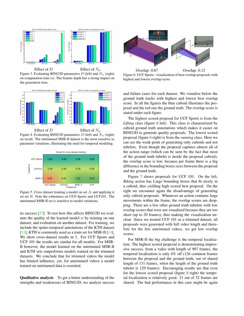
Qualitative analysis To get a better understanding of thestrengths and weaknesses of BING3D, we analyze success

Overlap: 0.87 Overlap: 0.12Figure 6. UCF Sports: visualization of best overlap proposals withhighest and lowest overlap score.

and failure cases for each dataset. We visualize below theground truth tracks with highest and lowest best overlapscore. In all the figures the blue cuboid illustrates the pro-posal and the red one the ground truth. The overlap score isstated under each figure.

The highest scored proposal for UCF Sports is from theLifting class (figure 6 left). This class is characterized bycuboid ground truth annotations which makes it easier onBING3D to generate quality proposals. The lowest scoredproposal (figure 6 right) is from the running class. Here wecan see the weak point of generating only cuboids and nottubelets. Even though the proposal captures almost all ofthe action range (which can be seen by the fact that mostof the ground truth tubelet is inside the proposal cuboid),the overlap score is low, because per frame there is a bigdifference in the bounding boxes sizes between the proposaland the ground truth.

Figure 7 shows proposals for UCF 101. On the left,Biking action has Large bounding boxes that fit nicely ina cuboid, thus yielding high scored best proposal. On theright we encounter again the disadvantage of generatingonly cuboid proposals. Whenever an action contains largemovements within the frame, the overlap scores are drop-ping. There are a few other ground truth tubelets with lowoverlap scores that were not visualized because they are tooshort (up to 20 frames), thus making the visualization un-clear. Since we treated UCF 101 as a trimmed dataset, allproposals were generated with full video length and there-fore for the few untrimmed videos, we get low overlapscores.

For MSR-II the big challenge is the temporal localiza-tion. The highest scored proposal is demonstrating impres-sive success, from a video with length of 907 frames, thetemporal localization is only 4% off (126 common framesbetween the proposal and the ground truth, out of sharedlength of 131 frames, when the length of the ground truthtubelet is 129 frames). Encouraging results are that evenfor the lowest scored proposal (figure 8 right) the tempo-ral localization is relatively good. 21 out of 32 frames areshared. The bad performance in this case might be again

Overlap: 0.81 Overlap: 0.05Figure 7. UCF 101: visualization of best overlap proposals withhighest and lowest overlap score.

Overlap: 0.84 Overlap: 0.29Figure 8. MSR-II: visualization of best overlap proposals withhighest and lowest overlap score.

Computation time (s)Pre-processing Generation Total

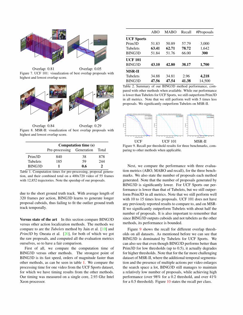
Prim3D 840 38 878Tubelets 185 59 244BING3D 1 0.6 2

Table 1. Computation times for pre-processing, proposal genera-tion, and their combined total on a 400x720 video of 55 frameswith 12,852 trajectories. Note the speedup of our proposals.

due to the short ground truth track. With average length of320 frames per action, BING3D learns to generate longerproposal cuboids, thus failing to fit the outlier ground truthtrack temporally.

Versus state of the art In this section compare BING3Dversus other action localization methods. The methods wecompare to are the Tubelets method by Jain et al. [10] andPrim3D by Oneata et al. [20], for both of which we gotthe raw proposals, and computed all the evaluation metricsourselves, so to have a fair comparison.

First of all, we compare the computation time ofBING3D versus other methods. The strongest point ofBING3D is its fast speed, orders of magnitude faster thanother methods, as can be seen in table 1. We compare theprocessing time for one video from the UCF Sports dataset,for which we have timing results from the other methods.Our timing was measured on a single core, 2.93 Ghz IntelXeon processor.

ABO MABO Recall #Proposals

UCF SportsPrim3D 51.83 50.89 57.79 3,000Tubelets 63.41 62.71 78.72 1,642BING3D 51.84 51.76 66.00 300

UCF 101BING3D 43.10 42.80 38.17 1,700

MSR-IITubelets 34.88 34.81 2.96 4,218BING3D 47.56 47.54 41.38 14,500

Table 2. Summary of our BING3D method performance, com-pared with other methods when available. While our performanceis lower than Tubelets for UCF Sports, we still outperform Prim3Din all metrics. Note that we still perform well with 5 times lessproposals. We significantly outperform Tubelets on MSR-II.

0 0.1 0.2 0.3 0.4 0.5 0.6 0.7 0.8 0.9 10

0.1

0.2

0.3

0.4

0.5

0.6

0.7

0.8

0.9

1UCF Sports: Recall per overlap threshold (150 actions)

Overlap threshold

% R

ecal

l

BING3DTubeletsPrim3D

0 0.1 0.2 0.3 0.4 0.5 0.6 0.7 0.8 0.9 10

0.1

0.2

0.3

0.4

0.5

0.6

0.7

0.8

0.9

1UCF 101: Recall per overlap threshold (3204 actions)

Overlap threshold

% R

ecal

l

BING3D

0 0.1 0.2 0.3 0.4 0.5 0.6 0.7 0.8 0.9 10

0.1

0.2

0.3

0.4

0.5

0.6

0.7

0.8

0.9

1MSR−II: Recall per overlap threshold (203 actions)

Overlap threshold

% R

ecal

l

BING3DTubelets

UCF UCF 101 MSR-IIFigure 9. Recall per threshold results for three benchmarks, com-paring to other methods when applicable.

Next, we compare the performance with three evalua-tion metrics (ABO, MABO and recall), for the three bench-marks. We also state the number of proposals each methodgenerated. Note that the number of proposals generated byBING3D is significantly lower. For UCF Sports our per-formance is lower than that of Tubelets, but we still outper-form Prim3D in all metrics. Note that we still perform wellwith 10 to 15 times less proposals. UCF 101 does not haveany previously reported results to compare to, and on MSR-II we significantly outperform Tubelets with about half thenumber of proposals. It is also important to remember thatsince BING3D outputs cuboids and not tubelets as the othermethods, its performance is bounded.

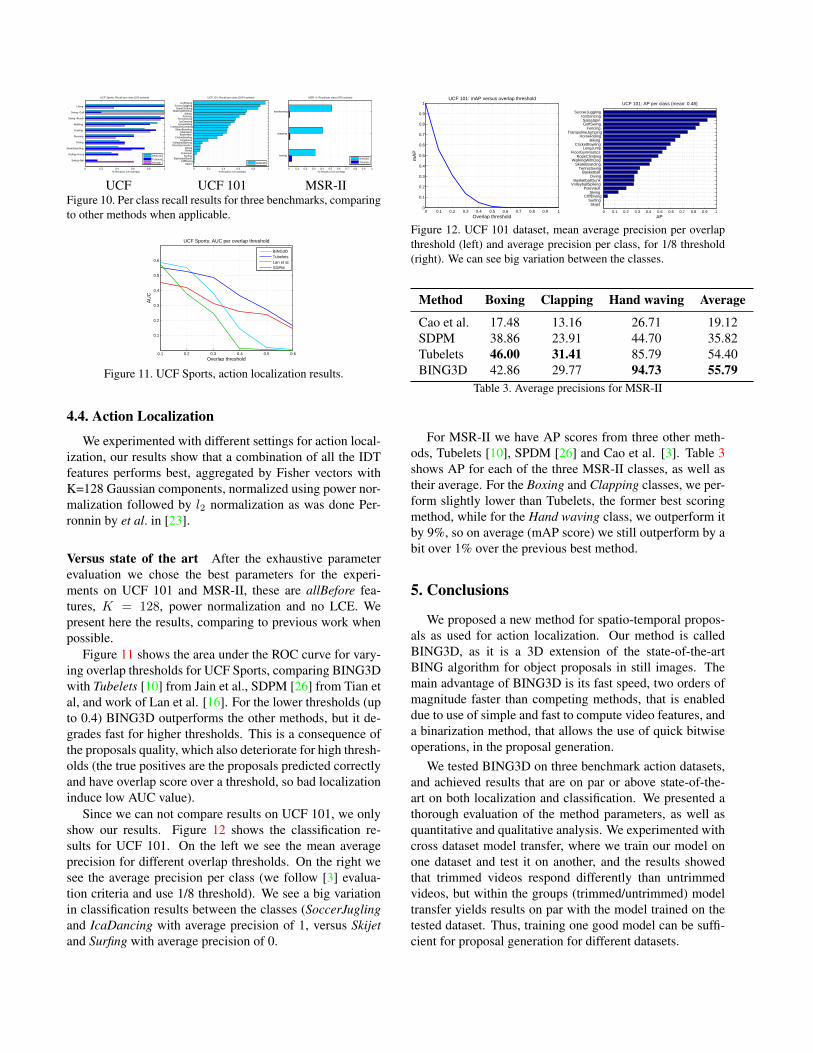
Figure 9 shows the recall for different overlap thresh-olds on all datasets. As mentioned before we can see thatBING3D is dominated by Tubelets for UCF Sports. Wecan also see that even though BING3D performs better thanPrim3D for low thresholds (up to 0.5), it actually degradesfor higher thresholds. Note that for the far more challengingdataset of MSR-II, where the additional temporal segmenta-tion and the presence of multiple actions per video enlargesthe search space a lot, BING3D still manages to maintaina relatively low number of proposals, while achieving highperformance (over 98% for a 0.2 threshold, and over 41%for a 0.5 threshold). Figure 10 states the recall per class.

0 0.2 0.4 0.6 0.8 1

Swing−Bar

Riding−Horse

SkateBoarding

Diving

Running

Kicking

Walking

Swing−Bench

Swing−Golf

Lifting

% Recall (≥ 0.5 overlap)

UCF Sports: Recall per class (150 actions)

BING3DTubeletsPrim3D

0 0.2 0.4 0.6 0.8 1

Skijet CliffDiving

BasketballDunk Surfing

PoleVault Skiing Diving

FloorGymnastics VolleyballSpiking

LongJump CricketBowling

Basketball SalsaSpin

SkateBoarding TrampolineJumping

HorseRiding IceDancing

TennisSwing Fencing

Biking WalkingWithDog

RopeClimbing SoccerJuggling

GolfSwing

% Recall (≥ 0.5 overlap)

UCF 101: Recall per class (3204 actions)

BING3D

0 0.1 0.2 0.3 0.4 0.5 0.6 0.7 0.8 0.9 1

boxing

clapping

handwaving

% Recall (≥ 0.5 overlap)

MSR−II: Recall per class (203 actions)

BING3DTubelets

UCF UCF 101 MSR-IIFigure 10. Per class recall results for three benchmarks, comparingto other methods when applicable.

0.1 0.2 0.3 0.4 0.5 0.6

0.1

0.2

0.3

0.4

0.5

0.6

Overlap threshold

AU

C

UCF Sports: AUC per overlap threshold

BING3DTubeletsLan et al.SDPM

Figure 11. UCF Sports, action localization results.

4.4. Action Localization

We experimented with different settings for action local-ization, our results show that a combination of all the IDTfeatures performs best, aggregated by Fisher vectors withK=128 Gaussian components, normalized using power nor-malization followed by l2 normalization as was done Per-ronnin by et al. in [23].

Versus state of the art After the exhaustive parameterevaluation we chose the best parameters for the experi-ments on UCF 101 and MSR-II, these are allBefore fea-tures, K = 128, power normalization and no LCE. Wepresent here the results, comparing to previous work whenpossible.

Figure 11 shows the area under the ROC curve for vary-ing overlap thresholds for UCF Sports, comparing BING3Dwith Tubelets [10] from Jain et al., SDPM [26] from Tian etal, and work of Lan et al. [16]. For the lower thresholds (upto 0.4) BING3D outperforms the other methods, but it de-grades fast for higher thresholds. This is a consequence ofthe proposals quality, which also deteriorate for high thresh-olds (the true positives are the proposals predicted correctlyand have overlap score over a threshold, so bad localizationinduce low AUC value).

Since we can not compare results on UCF 101, we onlyshow our results. Figure 12 shows the classification re-sults for UCF 101. On the left we see the mean averageprecision for different overlap thresholds. On the right wesee the average precision per class (we follow [3] evalua-tion criteria and use 1/8 threshold). We see a big variationin classification results between the classes (SoccerJuglingand IcaDancing with average precision of 1, versus Skijetand Surfing with average precision of 0.

0 0.1 0.2 0.3 0.4 0.5 0.6 0.7 0.8 0.9 10

0.1

0.2

0.3

0.4

0.5

0.6

0.7

0.8

0.9

1

Overlap threshold

mA

P

UCF 101: mAP versus overlap threshold

0 0.1 0.2 0.3 0.4 0.5 0.6 0.7 0.8 0.9 1

Skijet Surfing

CliffDiving Skiing

PoleVault VolleyballSpiking

BasketballDunk Diving

Basketball TennisSwing

SkateBoarding WalkingWithDog

RopeClimbing FloorGymnastics

LongJump CricketBowling

Biking HorseRiding

TrampolineJumping Fencing

GolfSwing SalsaSpin

IceDancing SoccerJuggling

AP

UCF 101: AP per class (mean: 0.48)

Figure 12. UCF 101 dataset, mean average precision per overlapthreshold (left) and average precision per class, for 1/8 threshold(right). We can see big variation between the classes.

Method Boxing Clapping Hand waving Average

Cao et al. 17.48 13.16 26.71 19.12SDPM 38.86 23.91 44.70 35.82Tubelets 46.00 31.41 85.79 54.40BING3D 42.86 29.77 94.73 55.79

Table 3. Average precisions for MSR-II

For MSR-II we have AP scores from three other meth-ods, Tubelets [10], SPDM [26] and Cao et al. [3]. Table 3shows AP for each of the three MSR-II classes, as well astheir average. For the Boxing and Clapping classes, we per-form slightly lower than Tubelets, the former best scoringmethod, while for the Hand waving class, we outperform itby 9%, so on average (mAP score) we still outperform by abit over 1% over the previous best method.

5. Conclusions

We proposed a new method for spatio-temporal propos-als as used for action localization. Our method is calledBING3D, as it is a 3D extension of the state-of-the-artBING algorithm for object proposals in still images. Themain advantage of BING3D is its fast speed, two orders ofmagnitude faster than competing methods, that is enableddue to use of simple and fast to compute video features, anda binarization method, that allows the use of quick bitwiseoperations, in the proposal generation.

We tested BING3D on three benchmark action datasets,and achieved results that are on par or above state-of-the-art on both localization and classification. We presented athorough evaluation of the method parameters, as well asquantitative and qualitative analysis. We experimented withcross dataset model transfer, where we train our model onone dataset and test it on another, and the results showedthat trimmed videos respond differently than untrimmedvideos, but within the groups (trimmed/untrimmed) modeltransfer yields results on par with the model trained on thetested dataset. Thus, training one good model can be suffi-cient for proposal generation for different datasets.

References[1] B. Alexe, T. Deselaers, and V. Ferrari. Measuring the object-

ness of image windows. TPAMI, 2012. 1, 2[2] M. V. D. Bergh, G. Roig, X. Boix, S. Manen, and L. V.

Gool. Online video seeds for temporal window objectness.In ICCV, 2013. 2

[3] L. Cao, Z. Liu, and T. S. Huang. Cross-dataset action detec-tion. In Computer vision and pattern recognition (CVPR),2010 IEEE conference on, pages 1998–2005. IEEE, 2010. 7

[4] M.-M. Cheng, Z. Zhang, W.-Y. Lin, and P. Torr. Bing: Bina-rized normed gradients for objectness estimation at 300fps.In CVPR, 2014. 1, 2, 3

[5] N. Dalal, B. Triggs, and C. Schmid. Human detection usingoriented histograms of flow and appearance. In ECCV, 2006.2

[6] I. Everts, J. C. van Gemert, and T. Gevers. Evaluation ofcolor spatio-temporal interest points for human action recog-nition. TIP, 23(4):1569–1580, 2014. 2

[7] R.-E. Fan, K.-W. Chang, C.-J. Hsieh, X.-R. Wang, and C.-J.Lin. LIBLINEAR: A library for large linear classification.Journal of Machine Learning Research, 9:1871–1874, 2008.4

[8] S. Hare, A. Saffari, and P. H. Torr. Efficient online structuredoutput learning for keypoint-based object tracking. In CVPR,2012. 3

[9] M. Jain, H. Jegou, and P. Bouthemy. Better exploiting mo-tion for better action recognition. In CVPR, 2013. 2

[10] M. Jain, J. C. van Gemert, H. Jegou, P. Bouthemy, andC. G. M. Snoek. Action localization with tubelets from mo-tion. In CVPR, 2014. 1, 2, 5, 6, 7

[11] Z. Jiang, Z. Lin, and L. S. Davis. Recognizing humanactions by learning and matching shape-motion prototypetrees. TPAMI, 34(3):533–547, 2012. 5

[12] Y. Ke, R. Sukthankar, and M. Hebert. Efficient visual eventdetection using volumetric features. In ICCV, 2011. 1, 2

[13] A. Klaser, M. Marszalek, and C. Schmid. A spatio-temporaldescriptor based on 3d-gradients. In BMVC, 2008. 2

[14] P. Krahenbuhl and V. Koltun. Geodesic object proposals. InECCV, 2014. 2

[15] C. H. Lampert, M. B. Blaschko, and T. Hofmann. Beyondsliding windows: Object localization by efficient subwindowsearch. In Computer Vision and Pattern Recognition, 2008.CVPR 2008. IEEE Conference on, pages 1–8. IEEE, 2008. 1

[16] T. Lan, Y. Wang, and G. Mori. Discriminative figure-centricmodels for joint action localization and recognition. In Com-puter Vision (ICCV), 2011 IEEE International Conferenceon, pages 2003–2010. IEEE, 2011. 4, 7

[17] I. Laptev and T. Lindeberg. Space-time interest points. InICCV, 2003. 2

[18] I. Laptev, M. Marzalek, C. Schmid, and B. Rozenfeld. Learn-ing realistic human actions from movies. In CVPR, 2008. 2

[19] S. Manen, M. Guillaumin, and L. V. Gool. Prime objectproposals with randomized prim’s algorithm. In ICCV, 2013.1, 2

[20] D. Oneata, J. Revaud, J. Verbeek, and C. Schmid. Spatio-temporal object detection proposals. In ECCV, 2014. 1, 2,6

[21] D. Oneata, J. Verbeek, and C. Schmid. Action and EventRecognition with Fisher Vectors on a Compact Feature Set.In ICCV, 2013. 2

[22] X. Peng, C. Zou, Y. Qiao, and Q. Peng. Action recognitionwith stacked fisher vectors. In ECCV, 2014. 2

[23] F. Perronnin, J. Sanchez, and T. Mensink. Improving thefisher kernel for large-scale image classification. In Com-puter Vision–ECCV 2010, pages 143–156. Springer, 2010.7

[24] M. D. Rodriguez, J. Ahmed, and M. Shah. Action mach:a spatio-temporal maximum average correlation height filterfor action recognition. In CVPR, 2008. 1, 2

[25] F. Shi, E. Petriu, and R. Laganiere. Sampling strategies forreal-time action recognition. In CVPR, 2013. 2

[26] Y. Tian, R. Sukthankar, and M. Shah. Spatiotemporal de-formable part models for action detection. In CVPR, 2013.1, 2, 7

[27] D. Tran and J. Yuan. Max-margin structured output regres-sion for spatio-temporal action localization. In NIPS, 2012.2

[28] D. Tran, J. Yuan, and D. Forsyth. Video event detection:From subvolume localization to spatio-temporal path search.TPAMI, 2013. 2

[29] J. R. Uijlings, K. E. van de Sande, T. Gevers, and A. W.Smeulders. Selective search for object recognition. IJCV,104(2):154–171, 2013. 1, 2

[30] J. C. van Gemert, M. Jain, E. Gati, and C. G. M. Snoek.APT: Action localization Proposals from dense Trajectories.In BMVC, 2015. 1

[31] H. Wang, A. Klaser, C. Schmid, and C.-L. Liu. Action recog-nition by dense trajectories. In CVPR, 2011. 2

[32] H. Wang, A. Klaser, C. Schmid, and C.-L. Liu. Dense tra-jectories and motion boundary descriptors for action recog-nition. International journal of computer vision, 103(1):60–79, 2013. 4

[33] H. Wang and C. Schmid. Action Recognition with ImprovedTrajectories. In ICCV, 2013. 2, 4

[34] G. Willems, T. Tuytelaars, and L. Van Gool. An efficientdense and scale-invariant spatio-temporal interest point de-tector. In ECCV, 2008. 2

[35] C. Xu and J. J. Corso. Evaluation of super-voxel methods forearly video processing. In CVPR, 2012. 1

[36] J. Yuan, Z. Liu, and Y. Wu. Discriminative subvolume searchfor efficient action detection. In CVPR, 2009. 2

[37] Q. Zhao, Z. Liu, and B. Yin. Cracking bing and beyond. InBMVC, 2014. 5

[38] C. L. Zitnick and P. Dollar. Edge boxes: Locating objectproposals from edges. In ECCV, 2014. 2