BINF733s2006 VisualizingData solka - UB · W. S. Cleveland, Visualizing Data. Hobart Press, Summit, New Jersey, 1993. W. S. Cleveland. The Elements of Graphing Data (Revised).Hobart

Copyright J.SolkaBINF733 Spring06 Solka/Weller -

Visualizing Data

Visualizing Data

BINF733 SPRING2006

Dr. Jeff Solka and Dr. Jennifer Weller

BINF733 Spring06 Solka/Weller -Visualizing Data

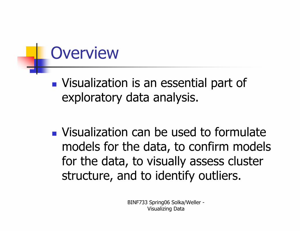
Overview

� Visualization is an essential part of exploratory data analysis.

� Visualization can be used to formulate models for the data, to confirm models for the data, to visually assess cluster structure, and to identify outliers.


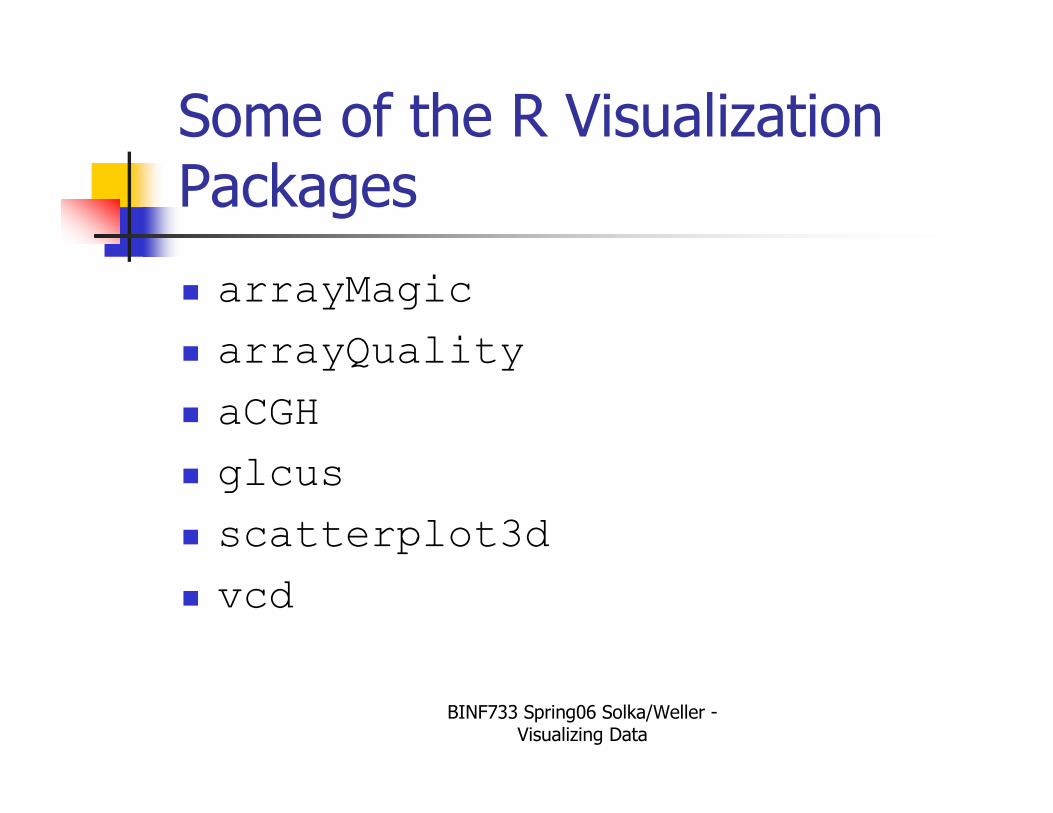
Some of the R Visualization Packages

� arrayMagic

� arrayQuality

� aCGH

� glcus

� scatterplot3d

� vcd


References - I

� J. Bertin. Semiologie Graphique. Walter de Gruyter, Inc., Berlin, 2 edition, 1973.

� W. S. Cleveland, Visualizing Data. Hobart Press, Summit, New Jersey, 1993.

� W. S. Cleveland. The Elements of Graphing Data (Revised). Hobart Press, Summit, New Jersey, 1994.

� E. Tufte. Envisioning Information (2e). Graphics Press, Cheshire, 1990.

� E. Tufte. The Visual Display of Quantitative Information (2e). Graphics Press Cheshire, 2001.


References - II

� Brewer, Cynthia A., 1996, Prediction of Simultaneous Contrast between Map Colors with Hunt’s Model of Color Appearance, Color Research and Application21(3): 221-235.

� Brewer, Cynthia A., 1994, Color Use Guidelines for Mapping and Visualization, Chapter 7 (pp. 123-147) in Visualization in Modern Cartography, edited by A.M. MacEachren and D.R.F. Taylor, Elsevier Science, Tarrytown, NY.


Color Space

� The work of Cynthia Brewer (1994a, b) discussed the fact that distances in color space should reflect quantitative distances between data.

� RColorBrewer


Interactive Graphics in R

� tcltk

� RGtk

� iSPlot

� GGobi

� Rggobi


High-volume Scatterplots

� D. B. Carr, R. J. Littlefield, W. L. Nicholson, and J. S. Littlefield. Scatterplot matrix techniques for large n. J. of the American Statistical Association, 82(398):424--436, 1987.


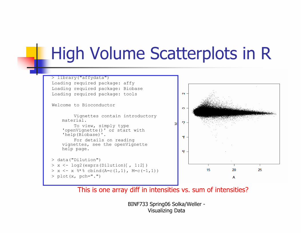
High Volume Scatterplots in R> library("affydata")

Loading required package: affy

Loading required package: Biobase

Loading required package: tools

Welcome to Bioconductor

Vignettes contain introductory material.

To view, simply type 'openVignette()' or start with 'help(Biobase)'.

For details on reading vignettes, see the openVignettehelp page.

> data("Dilution")

> x <- log2(exprs(Dilution)[, 1:2])

> x <- x %*% cbind(A=c(1,1), M=c(-1,1))

> plot(x, pch=".")

This is one array diff in intensities vs. sum of intensities?

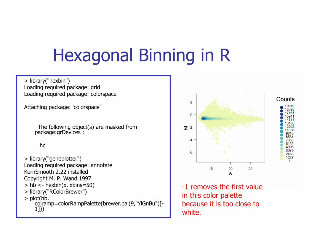
Hexagonal Binning in R

> library("hexbin")Loading required package: gridLoading required package: colorspace

Attaching package: 'colorspace'

The following object(s) are masked from package:grDevices :

hcl

> library("geneplotter")Loading required package: annotateKernSmooth 2.22 installedCopyright M. P. Wand 1997> hb <- hexbin(x, xbins=50)> library("RColorBrewer")> plot(hb,

colramp=colorRampPalette(brewer.pal(9,"YlGnBu")[-1]))

-1 removes the first value in this color palette because it is too close to white.


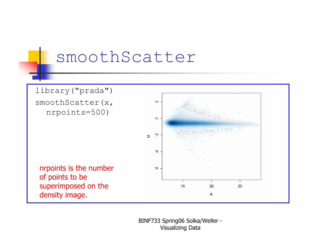
smoothScatter

library("prada")

smoothScatter(x,

nrpoints=500)

nrpoints is the number of points to be superimposed on the density image.


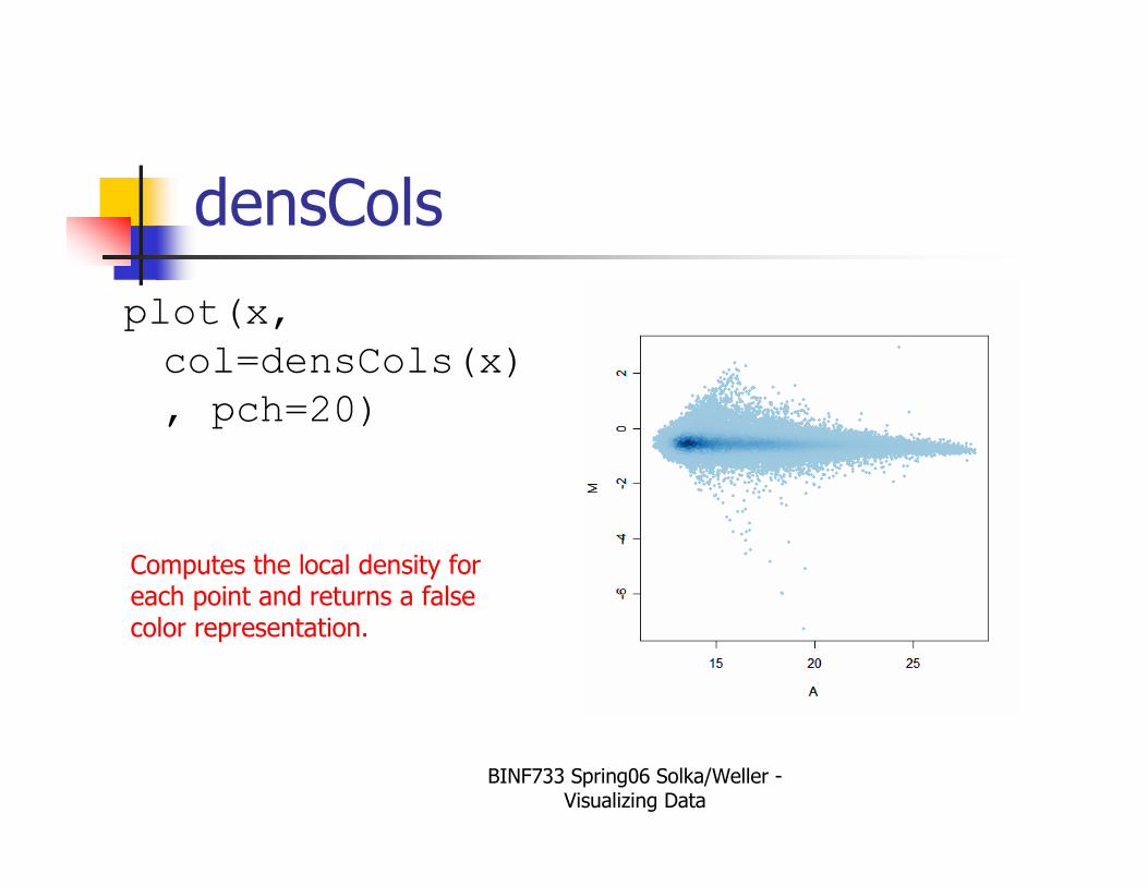
densCols

plot(x,

col=densCols(x)

, pch=20)

Computes the local density for each point and returns a false color representation.


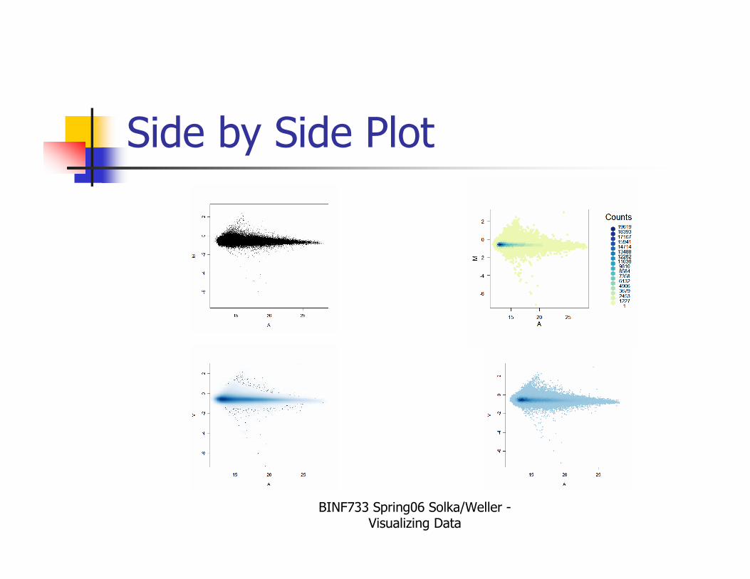
Side by Side Plot


A Few Notes on Performance

� pdf or ps files involving large numbers of points in a scatterplot can take a great deal of time to render.

� Advantages of binning� Long drawing times reduced once the bin counts have been computed

� A careful choice of bins can be used to replace observations prior to smoothing.� One can obtain good fitted curve performance assuming a decent choice of the bin locations.

� Smooth uses centers of bins as exemplars.


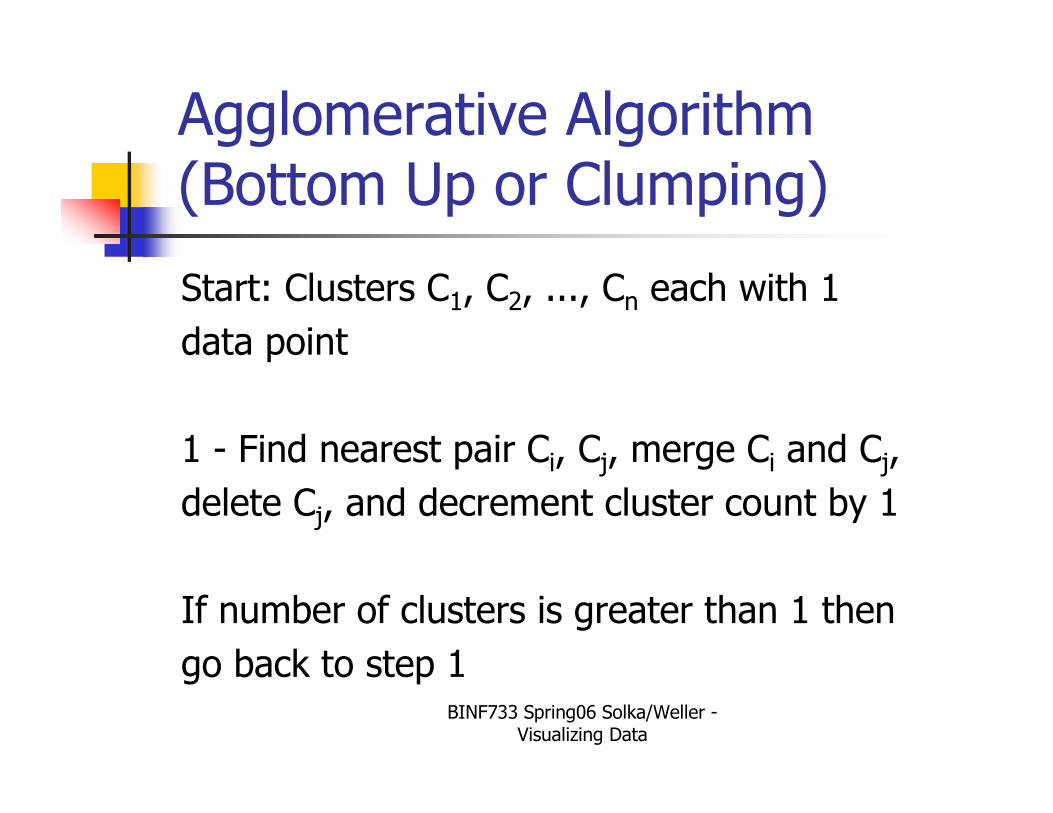
Agglomerative Algorithm(Bottom Up or Clumping)

Start: Clusters C1, C2, ..., Cn each with 1

data point

1 - Find nearest pair Ci, Cj, merge Ci and Cj,

delete Cj, and decrement cluster count by 1

If number of clusters is greater than 1 then

go back to step 1


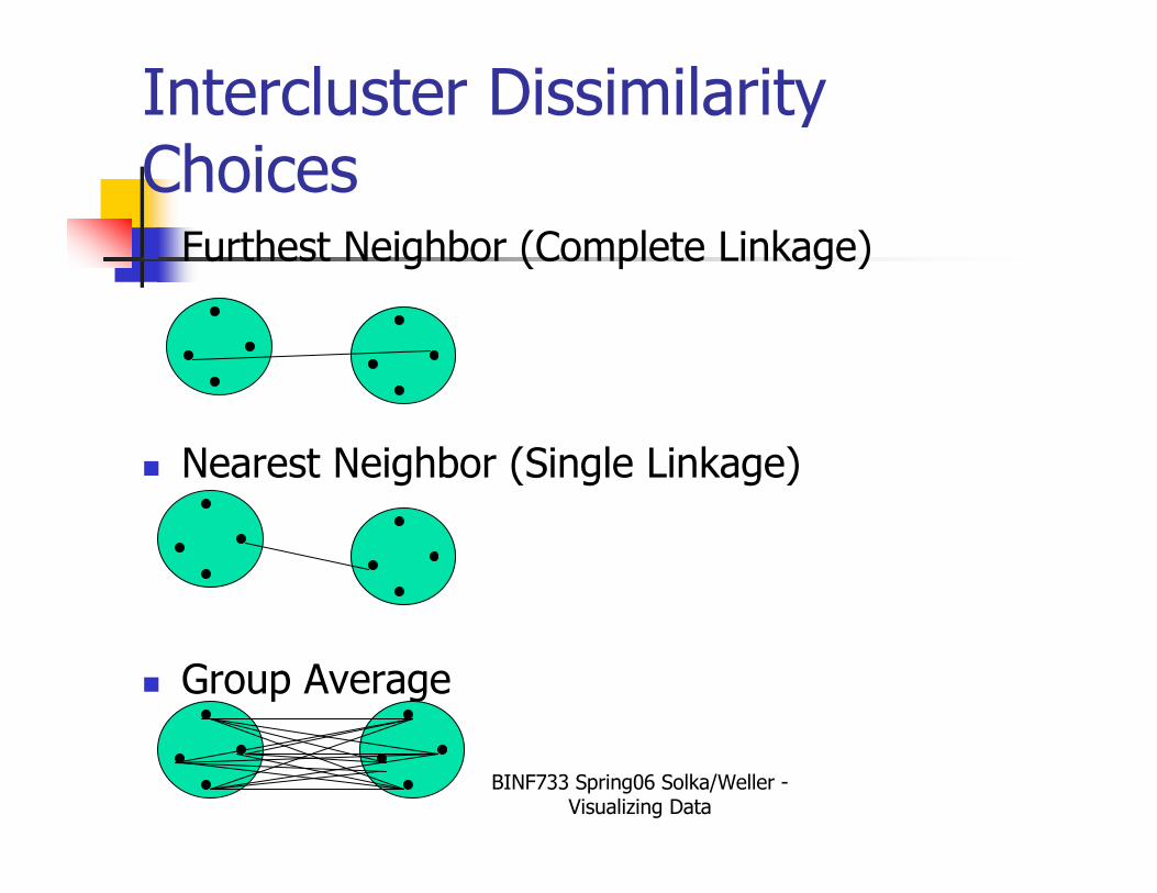
Intercluster Dissimilarity Choices� Furthest Neighbor (Complete Linkage)

� Nearest Neighbor (Single Linkage)

� Group Average


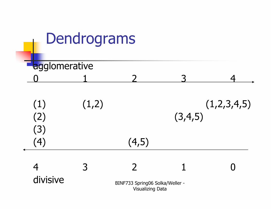
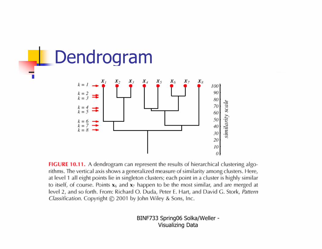
Dendrograms

agglomerative

0 1 2 3 4

(1) (1,2) (1,2,3,4,5)

(2) (3,4,5)

(3)

(4) (4,5)

4 3 2 1 0

divisive


Dendrogram


Heatmaps

� Eisen, MB., Spellman, PT., et al., (1998). Cluster analysis and display of genome-wide expression patterns. PNAS. 95:14863-14868.

� "The data image: a tool for exploring high dimensional data sets," Michael C. Minnotte and R. Webster West, 1998 Proceedings of the ASA Section on Statistical Graphics.

� E. Wegman. Hyperdimensional data analysis using parallel coordinates. Journal of the American Statistical Association, 85:664--675, 1990.

� Semiology of graphics (Hardcover) by Jacques Bertin, 1983


Heat Map (Data Imaging) Motivation

� How does one identify structure in large data sets in high dimensional space?

� Pairs plot

� n-dimensional data implies n x n plots

� Given a proposed clustering of such a data set then can one devise a method to allow the human visual system to assess the clustering?


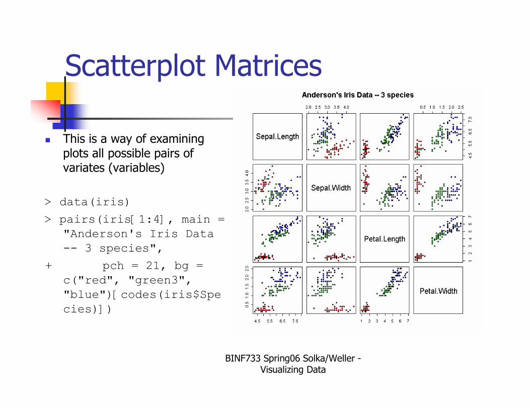
Scatterplot Matrices

� This is a way of examining plots all possible pairs of variates (variables)

> data(iris)

> pairs(iris[1:4], main =

"Anderson's Iris Data

-- 3 species",

+ pch = 21, bg =

c("red", "green3",

"blue")[codes(iris$Spe

cies)])


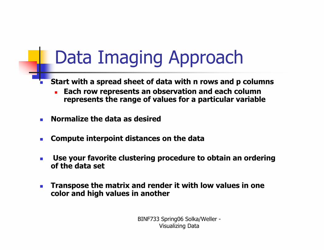
Data Imaging Approach� Start with a spread sheet of data with n rows and p columns

� Each row represents an observation and each column represents the range of values for a particular variable

� Normalize the data as desired

� Compute interpoint distances on the data

� Use your favorite clustering procedure to obtain an ordering of the data set

� Transpose the matrix and render it with low values in one color and high values in another

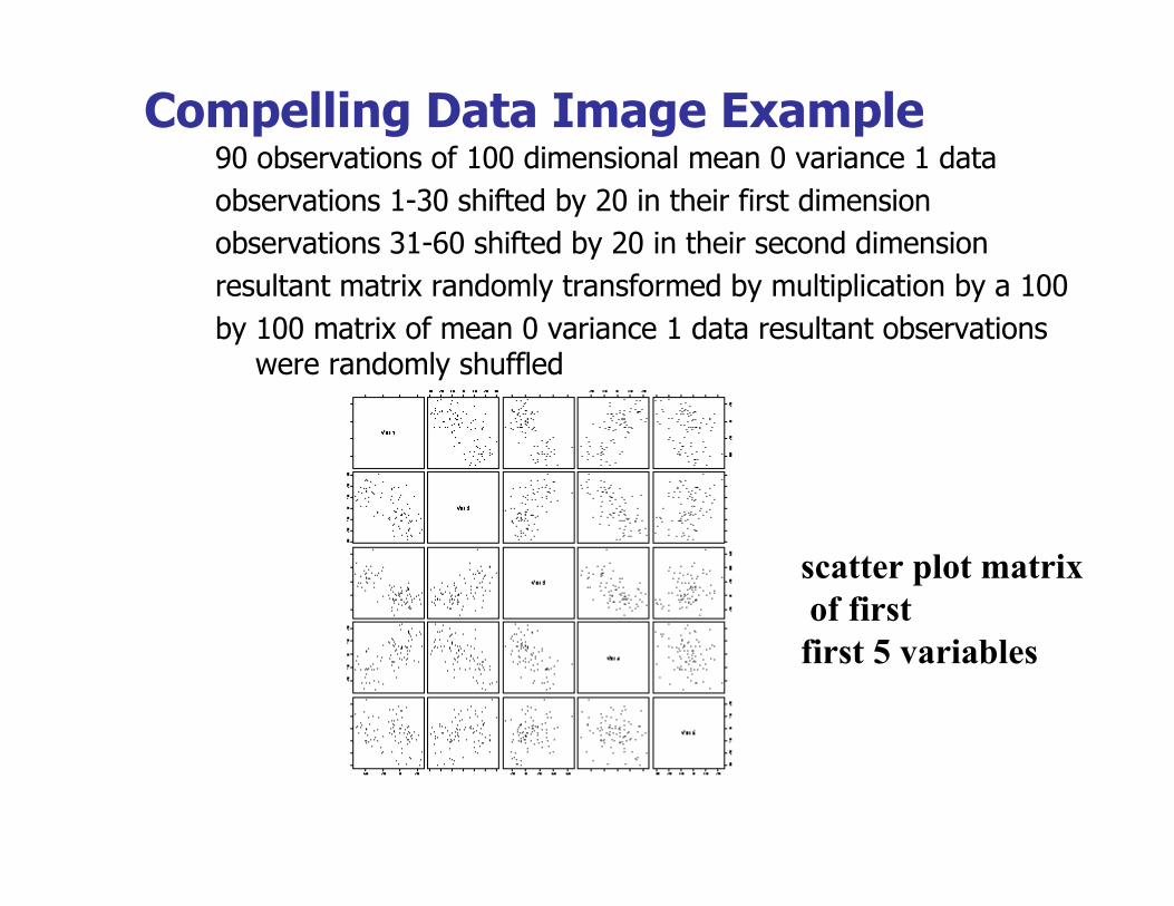
Compelling Data Image Example90 observations of 100 dimensional mean 0 variance 1 data

observations 1-30 shifted by 20 in their first dimension

observations 31-60 shifted by 20 in their second dimension

resultant matrix randomly transformed by multiplication by a 100

by 100 matrix of mean 0 variance 1 data resultant observations were randomly shuffled

scatter plot matrix

of first

first 5 variables


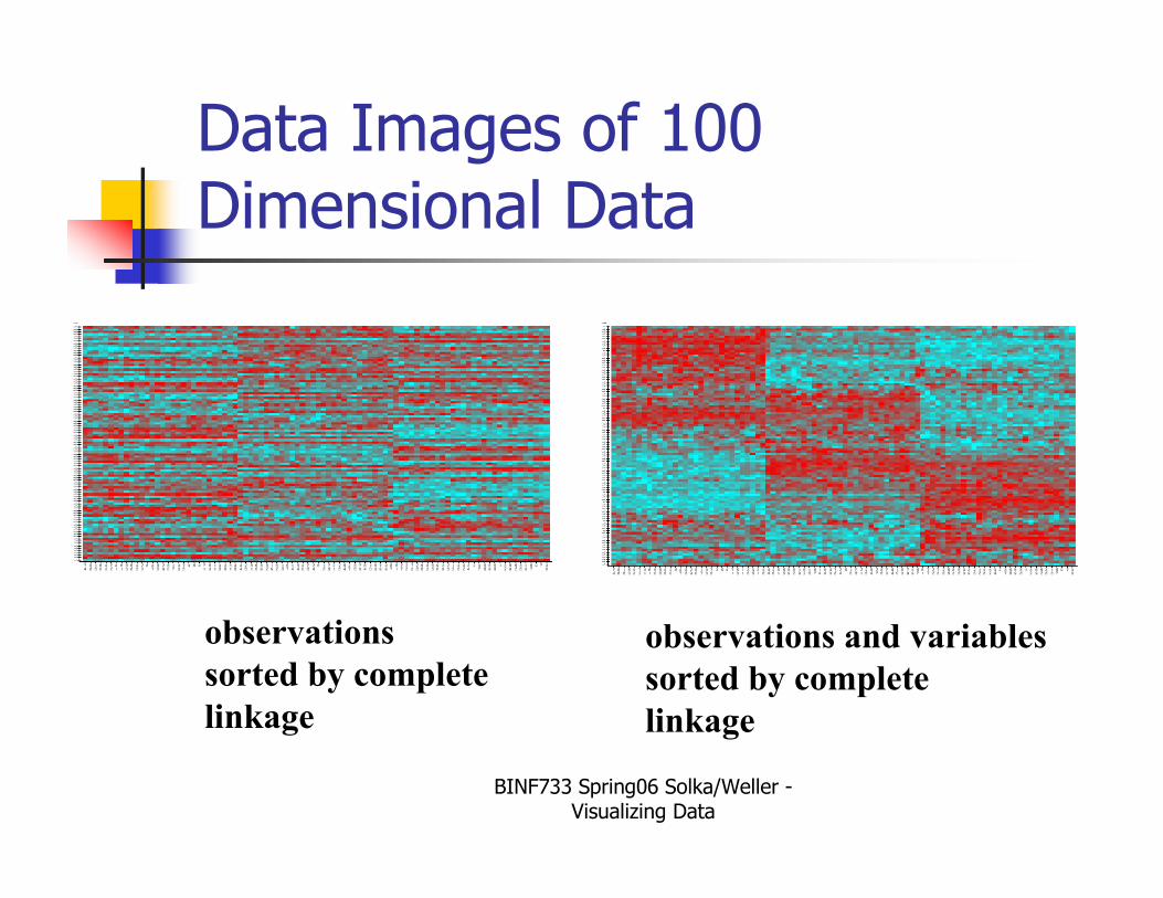
Data Images of 100 Dimensional Data

observations

sorted by complete

linkage

observations and variables

sorted by complete

linkage


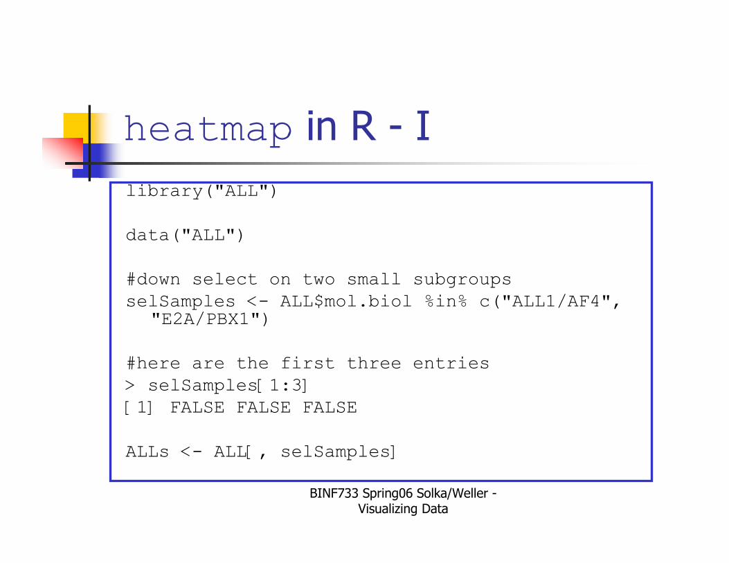
heatmap in R - I

library("ALL")

data("ALL")

#down select on two small subgroups

selSamples <- ALL$mol.biol %in% c("ALL1/AF4", "E2A/PBX1")

#here are the first three entries

> selSamples[1:3]

[1] FALSE FALSE FALSE

ALLs <- ALL[, selSamples]


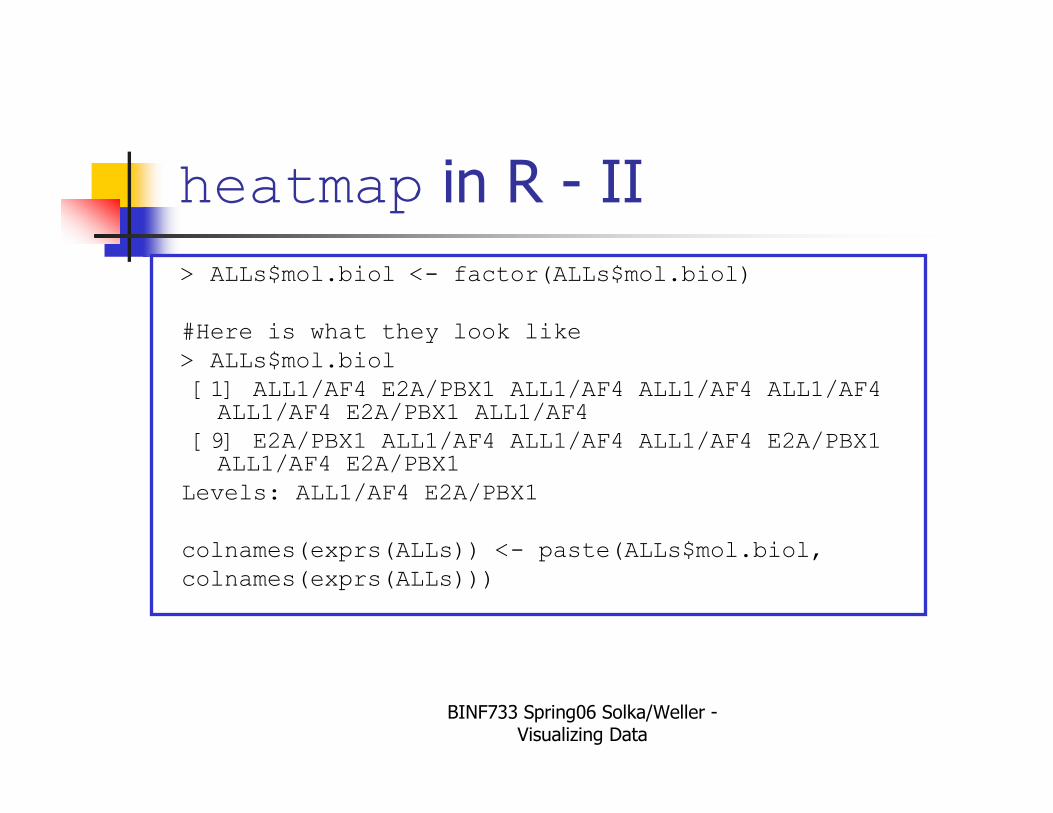
heatmap in R - II

> ALLs$mol.biol <- factor(ALLs$mol.biol)

#Here is what they look like

> ALLs$mol.biol

[1] ALL1/AF4 E2A/PBX1 ALL1/AF4 ALL1/AF4 ALL1/AF4 ALL1/AF4 E2A/PBX1 ALL1/AF4

[9] E2A/PBX1 ALL1/AF4 ALL1/AF4 ALL1/AF4 E2A/PBX1 ALL1/AF4 E2A/PBX1

Levels: ALL1/AF4 E2A/PBX1

colnames(exprs(ALLs)) <- paste(ALLs$mol.biol,

colnames(exprs(ALLs)))


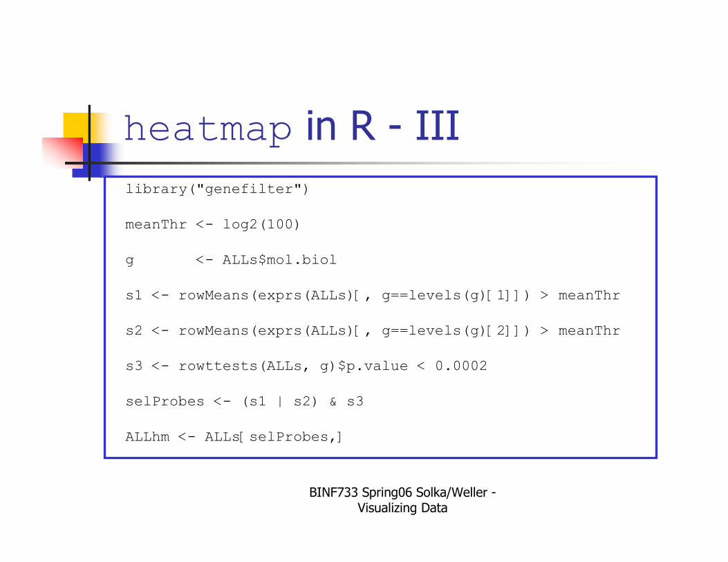
heatmap in R - III

library("genefilter")

meanThr <- log2(100)

g <- ALLs$mol.biol

s1 <- rowMeans(exprs(ALLs)[, g==levels(g)[1]]) > meanThr

s2 <- rowMeans(exprs(ALLs)[, g==levels(g)[2]]) > meanThr

s3 <- rowttests(ALLs, g)$p.value < 0.0002

selProbes <- (s1 | s2) & s3

ALLhm <- ALLs[selProbes,]


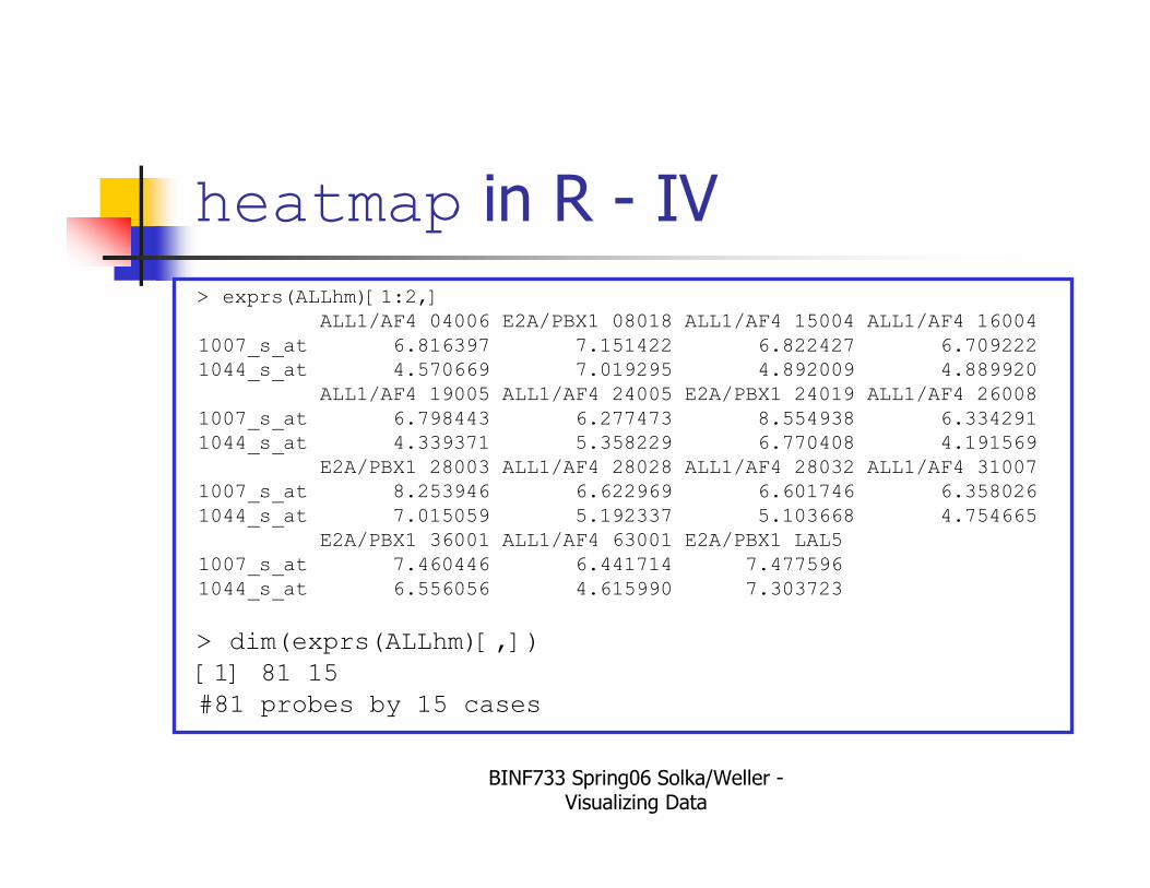
heatmap in R - IV

> exprs(ALLhm)[1:2,]ALL1/AF4 04006 E2A/PBX1 08018 ALL1/AF4 15004 ALL1/AF4 16004

1007_s_at 6.816397 7.151422 6.822427 6.7092221044_s_at 4.570669 7.019295 4.892009 4.889920

ALL1/AF4 19005 ALL1/AF4 24005 E2A/PBX1 24019 ALL1/AF4 26008

1007_s_at 6.798443 6.277473 8.554938 6.3342911044_s_at 4.339371 5.358229 6.770408 4.191569

E2A/PBX1 28003 ALL1/AF4 28028 ALL1/AF4 28032 ALL1/AF4 310071007_s_at 8.253946 6.622969 6.601746 6.358026

1044_s_at 7.015059 5.192337 5.103668 4.754665E2A/PBX1 36001 ALL1/AF4 63001 E2A/PBX1 LAL5

1007_s_at 7.460446 6.441714 7.477596

1044_s_at 6.556056 4.615990 7.303723

> dim(exprs(ALLhm)[,])

[1] 81 15

#81 probes by 15 cases


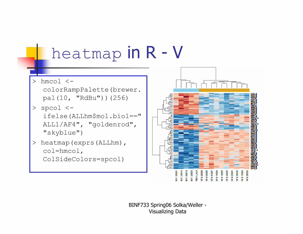
heatmap in R - V

> hmcol <-

colorRampPalette(brewer.

pal(10, "RdBu"))(256)

> spcol <-

ifelse(ALLhm$mol.biol=="

ALL1/AF4", "goldenrod",

"skyblue")

> heatmap(exprs(ALLhm),

col=hmcol,

ColSideColors=spcol)


Heatmaps of Residuals - I

� Y = f(x) + ε� Y is the observed data and x are the explanatory variables.

� An examination of the residuals can often leads to insights into the nature of the fit.

ˆˆ Y fε = −


Heatmaps of Residuals - II

� estrogen data

� 8 samples from and estrogen positive breast cancer cell line

� After serum starvation four samples were exposed to estrogen and then harvested for analysis with Affymetrix human genome U-95Av2 after 10 hours for two samples and 48 hours for the other two.


Heatmaps of Residuals - III

� For each probe set we have

� 8 measurements

� 4 coefficients

� Overall baseline

� Estrogen stimulation (+ = yes, - = no)

� Time effect (10h, 48h)

� Interaction between treatment and time

� Difference in treatment effect between 10h and 48h

� This leaves four residual degrees of freedom for each probe set


Heatmaps of Residuals - IV

� So we wish to compare the expression values that are computed by our model against the actual expression values.


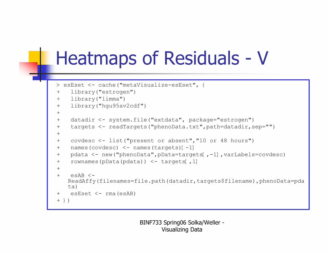
Heatmaps of Residuals - V> esEset <- cache("metaVisualize-esEset", {+ library("estrogen")

+ library("limma")+ library("hgu95av2cdf")

+

+ datadir <- system.file("extdata", package="estrogen")+ targets <- readTargets("phenoData.txt",path=datadir,sep="")

+ + covdesc <- list("present or absent","10 or 48 hours")

+ names(covdesc) <- names(targets)[-1]+ pdata <- new("phenoData",pData=targets[,-1],varLabels=covdesc)

+ rownames(pData(pdata)) <- targets[,1]

+ + esAB <-

ReadAffy(filenames=file.path(datadir,targets$filename),phenoData=pdata)

+ esEset <- rma(esAB)+ })


Heatmaps of Residuals - VI

Loading required package: hgu95av2

Loading required package:

hgu95av2cdf

Loading required package: vsn

Background correcting

Normalizing

Calculating Expression


Heatmaps of Residuals - VII

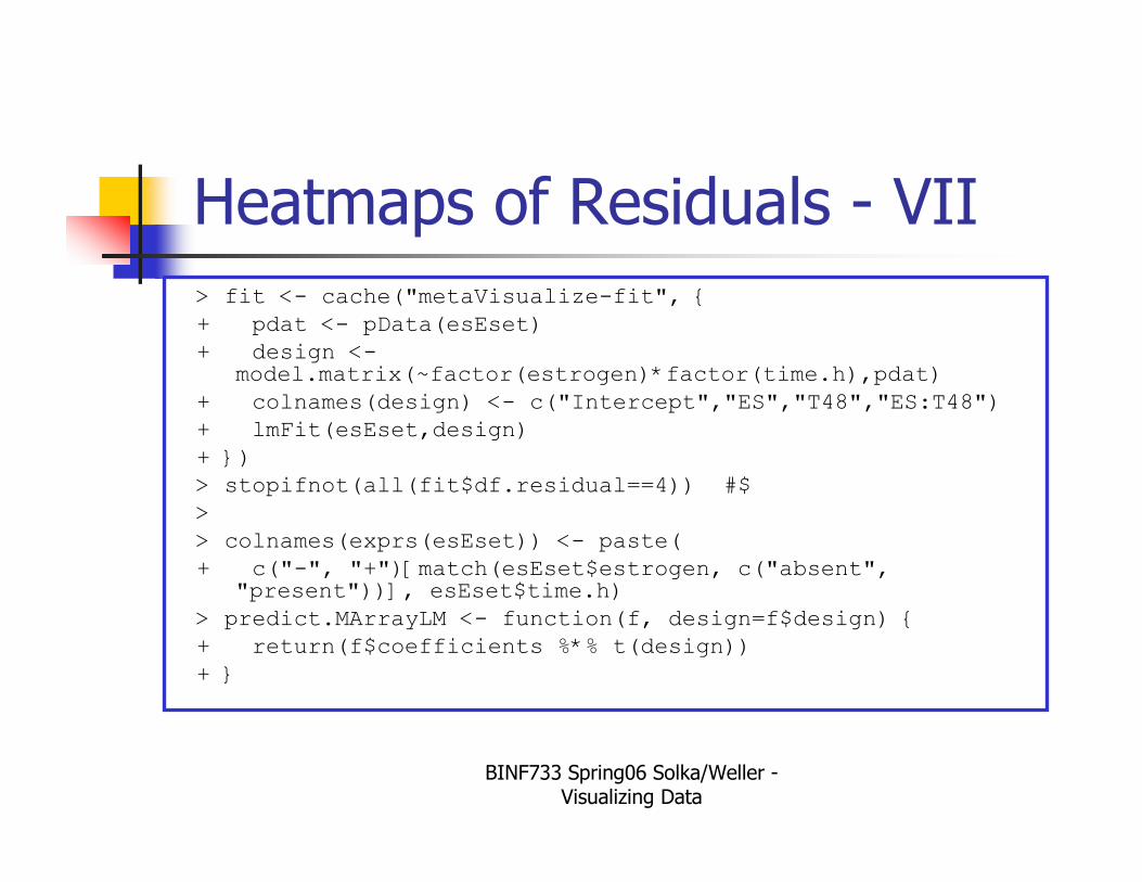
> fit <- cache("metaVisualize-fit", {

+ pdat <- pData(esEset)

+ design <-model.matrix(~factor(estrogen)*factor(time.h),pdat)

+ colnames(design) <- c("Intercept","ES","T48","ES:T48")

+ lmFit(esEset,design)

+ })

> stopifnot(all(fit$df.residual==4)) #$

>

> colnames(exprs(esEset)) <- paste(

+ c("-", "+")[match(esEset$estrogen, c("absent", "present"))], esEset$time.h)

> predict.MArrayLM <- function(f, design=f$design) {

+ return(f$coefficients %*% t(design))

+ }


Heatmaps of Residuals - VIII

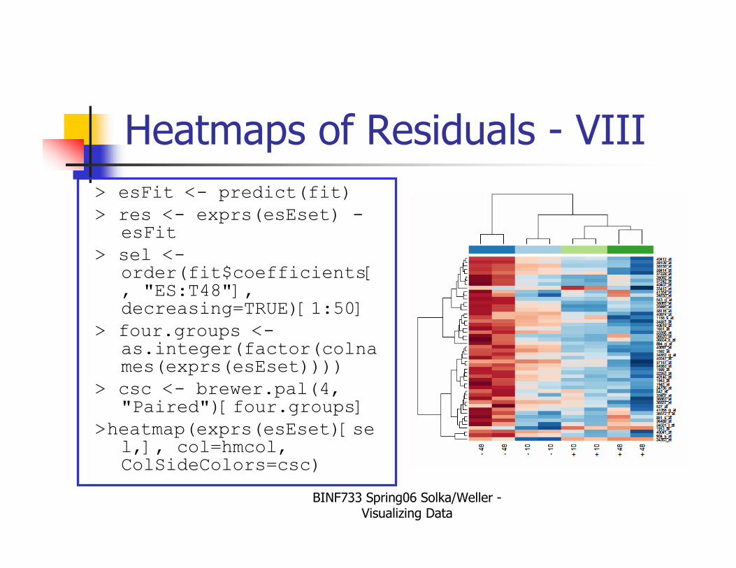
> esFit <- predict(fit)

> res <- exprs(esEset) -esFit

> sel <-order(fit$coefficients[, "ES:T48"], decreasing=TRUE)[1:50]

> four.groups <-as.integer(factor(colnames(exprs(esEset))))

> csc <- brewer.pal(4, "Paired")[four.groups]

>heatmap(exprs(esEset)[sel,], col=hmcol, ColSideColors=csc)


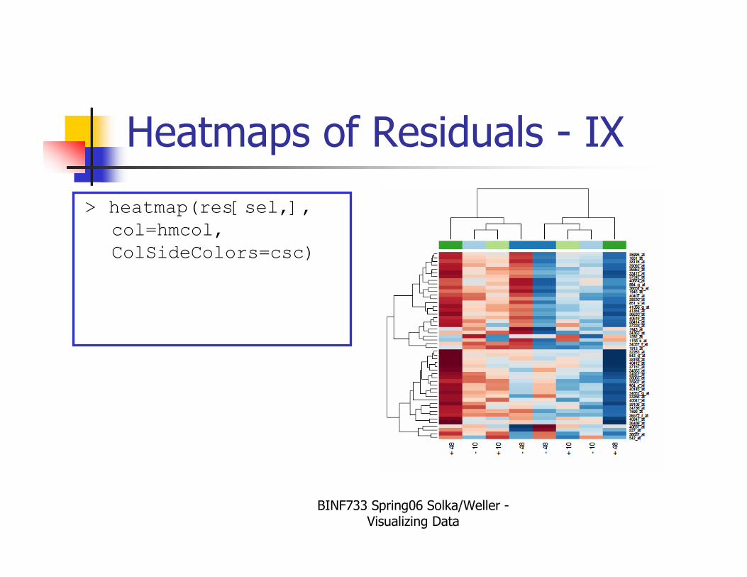
Heatmaps of Residuals - IX

> heatmap(res[sel,],

col=hmcol,

ColSideColors=csc)


Visualizing Distances

� We will have much more to say about distances and clustering/dendrograms later.

� Dendrograms impose an ordering on the data based on the sequence of merges in hierarchical agglomerative clustering.

� Cophenetic correlation can be used to measure the association between two different distance measures.� cophenetic in R


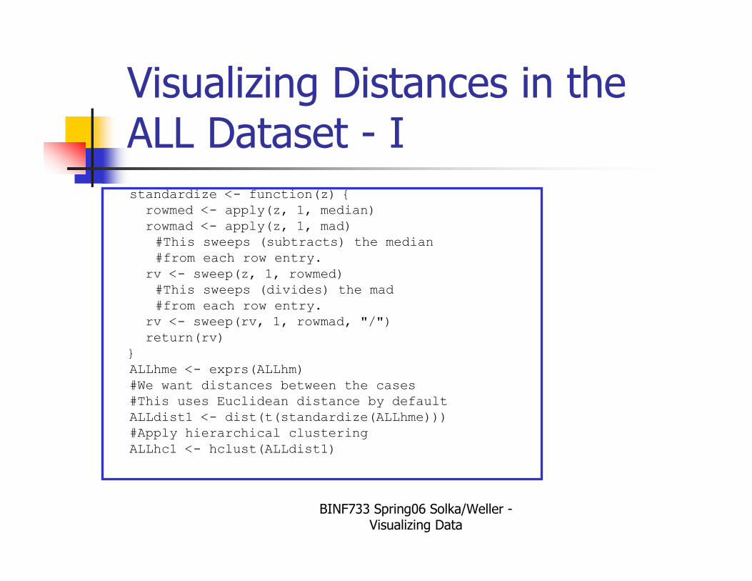
Visualizing Distances in the ALL Dataset - Istandardize <- function(z) {rowmed <- apply(z, 1, median)

rowmad <- apply(z, 1, mad)#This sweeps (subtracts) the median

#from each row entry.

rv <- sweep(z, 1, rowmed)#This sweeps (divides) the mad

#from each row entry.rv <- sweep(rv, 1, rowmad, "/")

return(rv)}

ALLhme <- exprs(ALLhm)

#We want distances between the cases#This uses Euclidean distance by default

ALLdist1 <- dist(t(standardize(ALLhme)))#Apply hierarchical clustering

ALLhc1 <- hclust(ALLdist1)


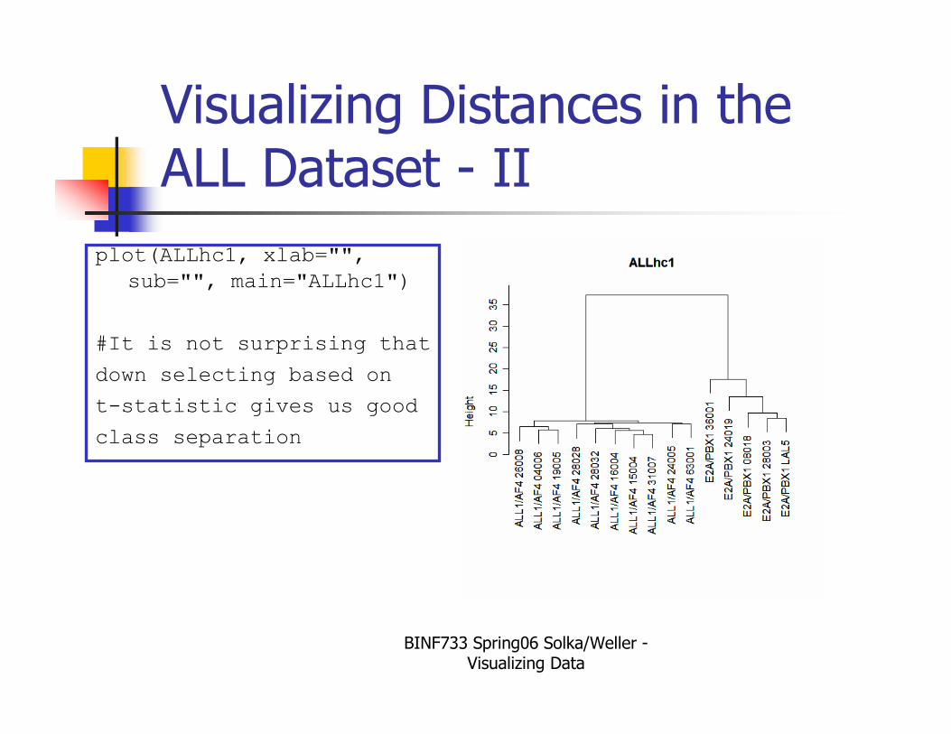
Visualizing Distances in the ALL Dataset - II

plot(ALLhc1, xlab="",

sub="", main="ALLhc1")

#It is not surprising that

down selecting based on

t-statistic gives us good

class separation


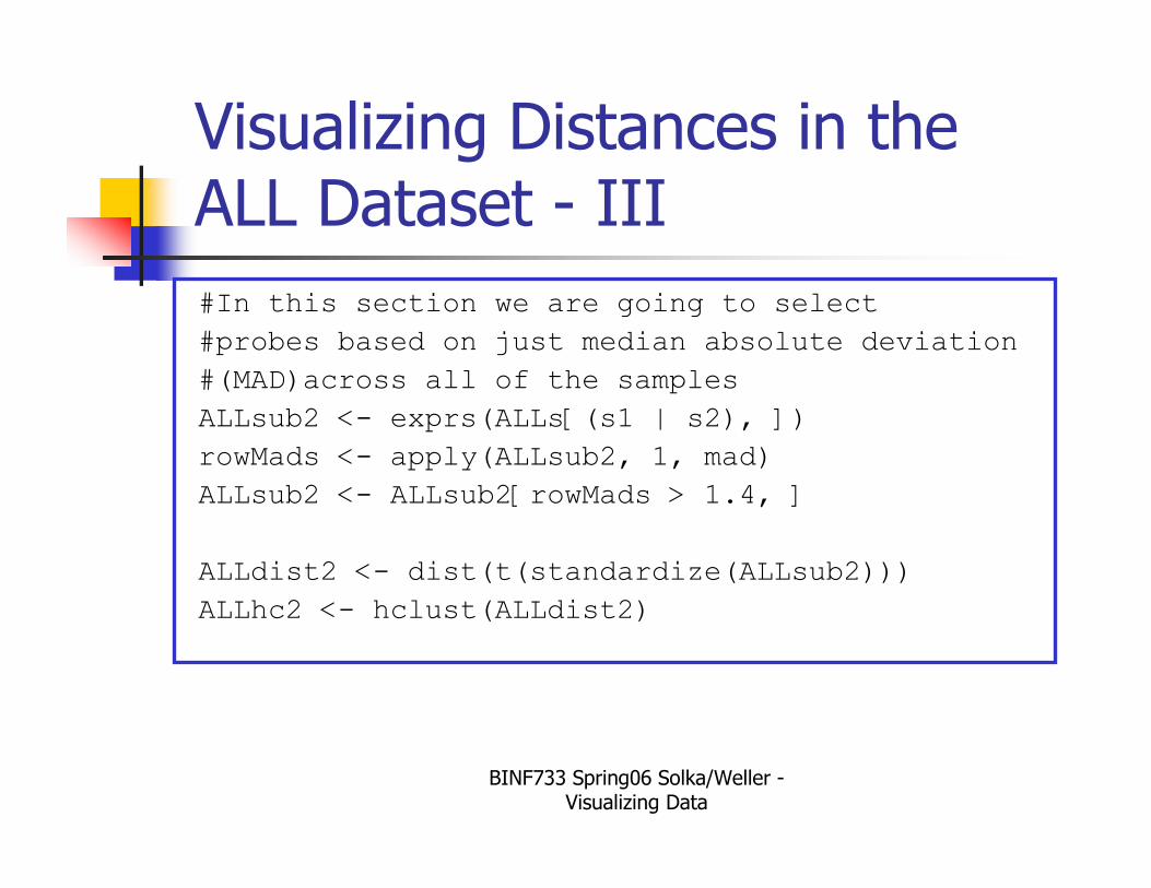
Visualizing Distances in the ALL Dataset - III

#In this section we are going to select

#probes based on just median absolute deviation

#(MAD)across all of the samples

ALLsub2 <- exprs(ALLs[(s1 | s2), ])

rowMads <- apply(ALLsub2, 1, mad)

ALLsub2 <- ALLsub2[rowMads > 1.4, ]

ALLdist2 <- dist(t(standardize(ALLsub2)))

ALLhc2 <- hclust(ALLdist2)


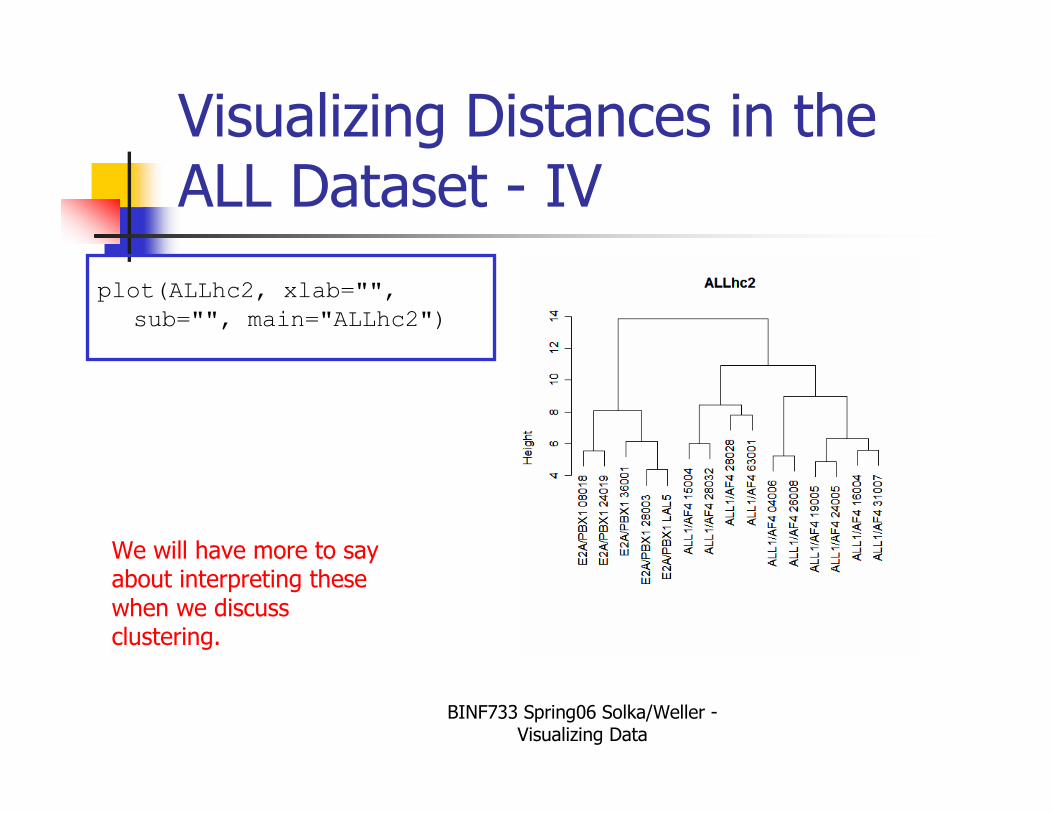
Visualizing Distances in the ALL Dataset - IV

plot(ALLhc2, xlab="",

sub="", main="ALLhc2")

We will have more to say about interpreting these when we discuss clustering.


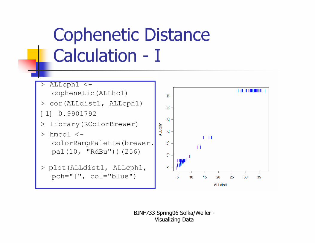
Cophenetic Distance Calculation - I

> ALLcph1 <-

cophenetic(ALLhc1)

> cor(ALLdist1, ALLcph1)

[1] 0.9901792

> library(RColorBrewer)

> hmcol <-

colorRampPalette(brewer.

pal(10, "RdBu"))(256)

> plot(ALLdist1, ALLcph1,

pch="|", col="blue")


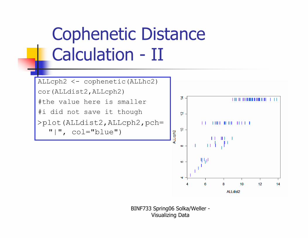
Cophenetic Distance Calculation - II

ALLcph2 <- cophenetic(ALLhc2)

cor(ALLdist2,ALLcph2)

#the value here is smaller

#i did not save it though

>plot(ALLdist2,ALLcph2,pch=

"|", col="blue")


Multi-dimensional Scaling (MDS)

� How can we evaluate the results of clustering high-dimensional observations?

� The dissimilarity measure that we used may not be a metric.

� We can’t draw a picture of the clustering in the high-dimensional space.

� Can we project to a lower dimensional space while preserving the distance relationships among the observations.

� This is the focus of multidimensional scaling (MDS)


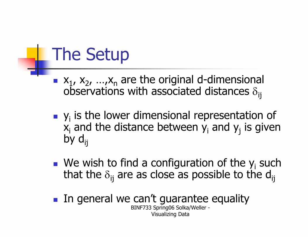
The Setup

� x1, x2, …,xn are the original d-dimensional observations with associated distances δij

� yi is the lower dimensional representation of xi and the distance between yi and yj is given by dij

� We wish to find a configuration of the yi such that the δij are as close as possible to the dij

� In general we can’t guarantee equality

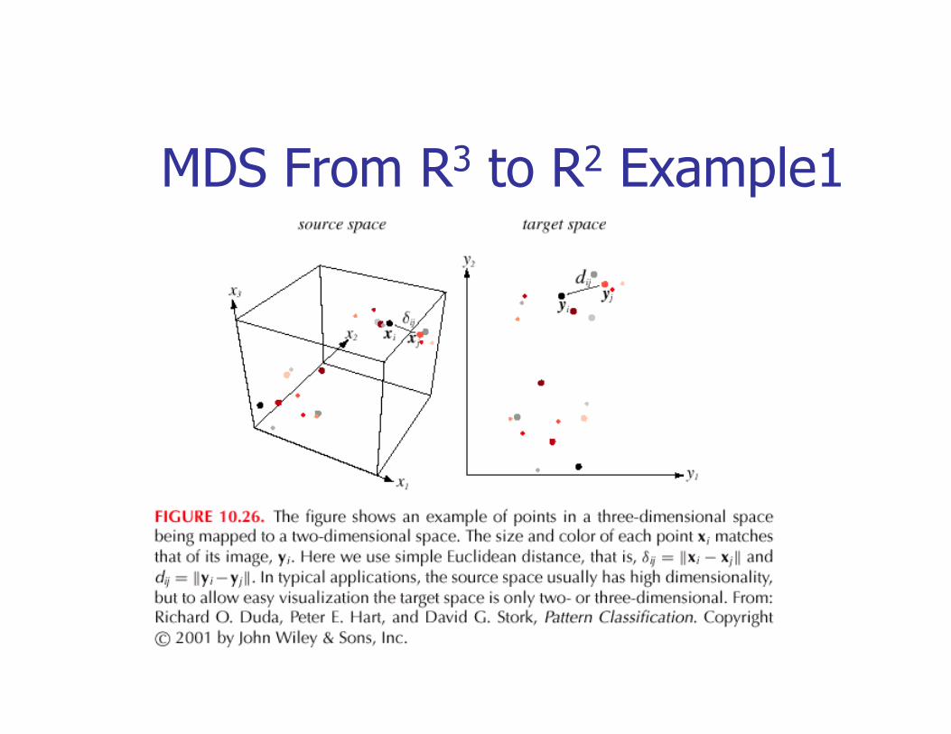
MDS From R3 to R2 Example1


MDS Criteria Functions

( )∑

∑<

<−

=ji ij

ji ijij

ee

dJ

2

2

δ

δ

2

∑<

−=

ji ij

ijij

ff

dJ

δ

δ

( )∑∑ <<

−=

ji ij

ijij

ji ij

ef

dJ

δ

δ

δ

21

• All criteria are invariant to rigid body

motions of the points

•Invariant to dilations of the points

•Jee emphasizes errors regardless of the

size of the δij

•Jff emphasizes large fraction errors

regardless of whether |δij - dij| is large or

small

•Jef is a compromise


MDS Procedure

� Choose Criteria

� Choose an initial configuration of the yi’s� Randomly

� Based on the coordinates with the largest variance

� Move the points in the direction of the greatest decrease in the criteria function

d̂


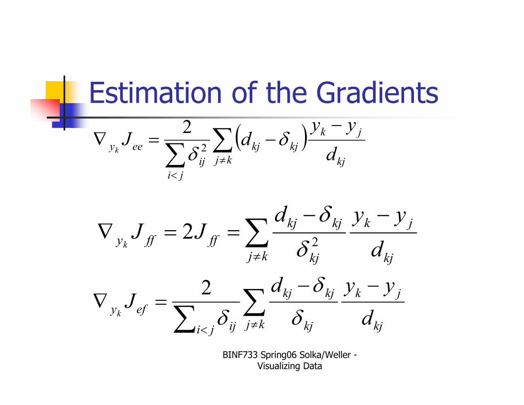
Estimation of the Gradients

( )∑∑ ≠<

−−=∇

kj kj

jk

kjkj

ji

ij

eeyd

yydJ

kδ

δ 2

2

kj

jk

kj kj

kjkj

ffffyd

yydJJ

k

−−==∇ ∑

≠2

2δ

δ

kj

jk

kj kj

kjkj

ji ij

efyd

yydJ

k

−−=∇ ∑∑ ≠<

δ

δ

δ2


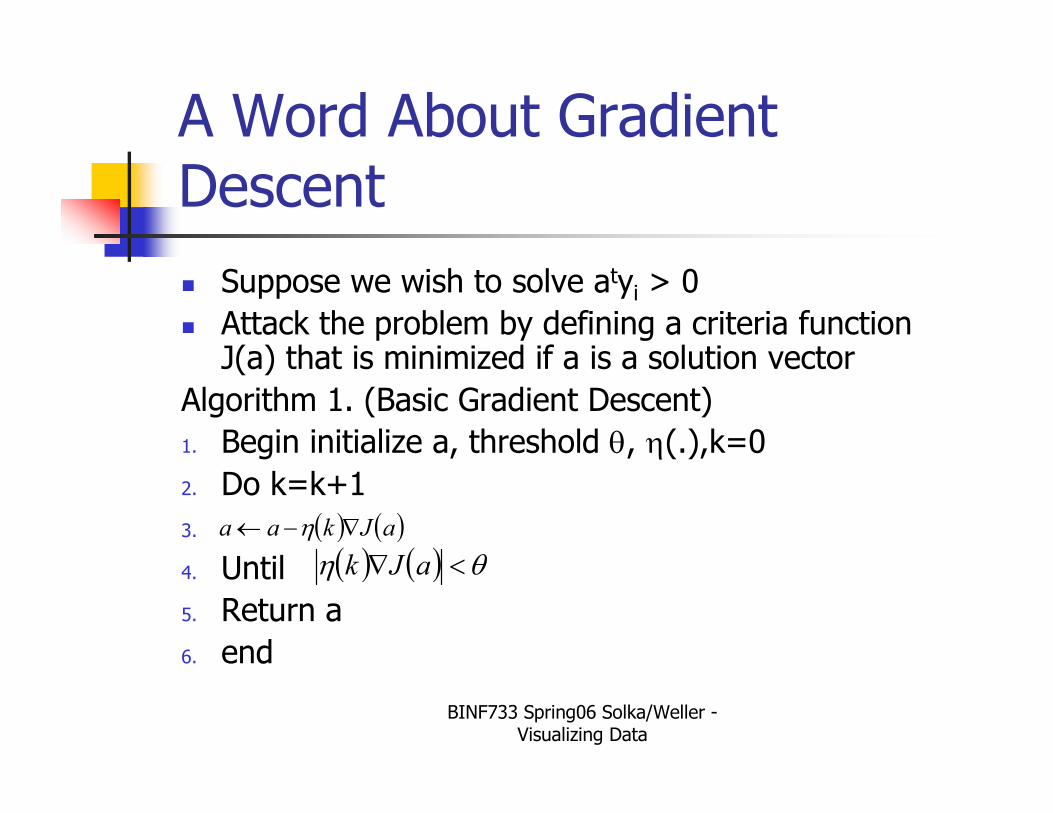
A Word About Gradient Descent

� Suppose we wish to solve atyi > 0

� Attack the problem by defining a criteria function J(a) that is minimized if a is a solution vector

Algorithm 1. (Basic Gradient Descent)

1. Begin initialize a, threshold θ, η(.),k=02. Do k=k+1

3.

4. Until

5. Return a

6. end

( ) ( )aJkaa ∇−← η

( ) ( ) θη <∇ aJk


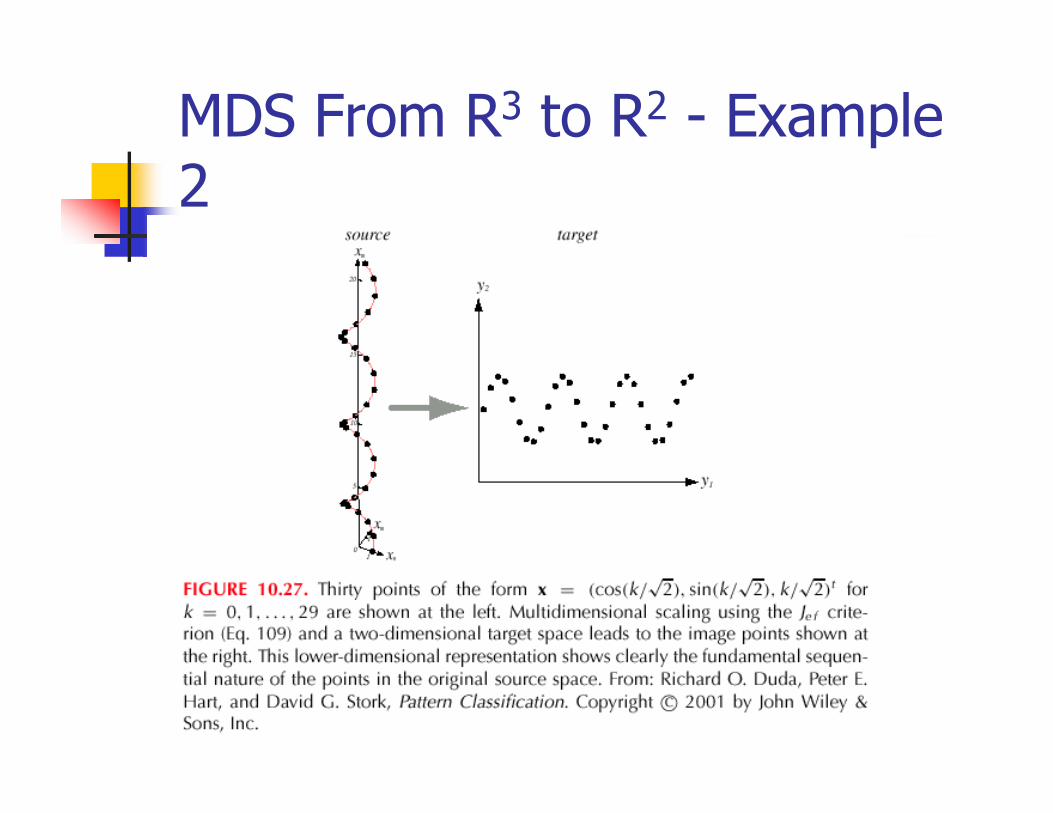
MDS From R3 to R2 - Example 2


Classical Multidimensional Scaling in R - I

� cmdscale in stats package

� Uses classical MDS with a least squares definition of energy Jee

� Computes a singular value decomposition of the double centered matrix of squared distances

� Solutions are nested (first two dimensions in k = 3 match the k = 2 solutions)


Classical Multidimensional Scaling in R - II

� Goodness of fit (GOF)

� For each dimension

� Sum of the eigenvalues for the components S divided by the sum of the absolute value of all eigenvalues

� Sum of the eigenvalues for the components S divided by the sum of all positive eigenvalues

� Examine scree plot and look for the elbow in the curve


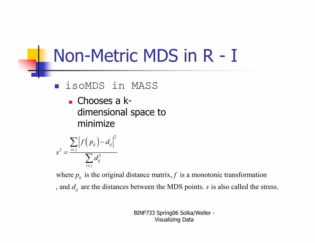
Non-Metric MDS in R - I

� isoMDS in MASS

� Chooses a k-dimensional space to minimize

( )2

2

2

where is the original distance matrix, is a monotonic transformation

, and are the distances between the MDS points. is also called the stress.

ij ij

i j

ij

i j

ij

ij

f p d

sd

p f

d s

≠

≠

−

=∑

∑


Non-Metric MDS in R - II

� sammon in MASS

� Uses a different loss function.


cmdscale and sammon in R

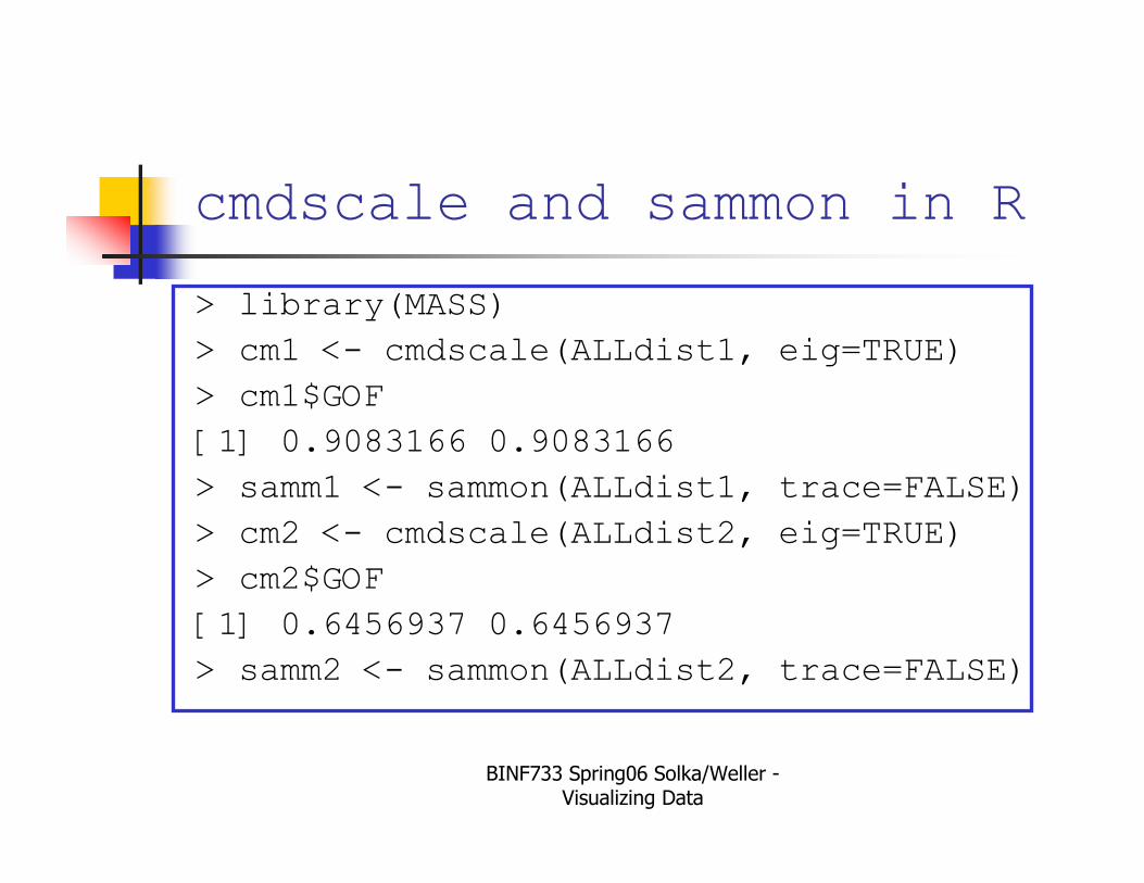
> library(MASS)

> cm1 <- cmdscale(ALLdist1, eig=TRUE)

> cm1$GOF

[1] 0.9083166 0.9083166

> samm1 <- sammon(ALLdist1, trace=FALSE)

> cm2 <- cmdscale(ALLdist2, eig=TRUE)

> cm2$GOF

[1] 0.6456937 0.6456937

> samm2 <- sammon(ALLdist2, trace=FALSE)


Setting Up Colors for the MDS Plots

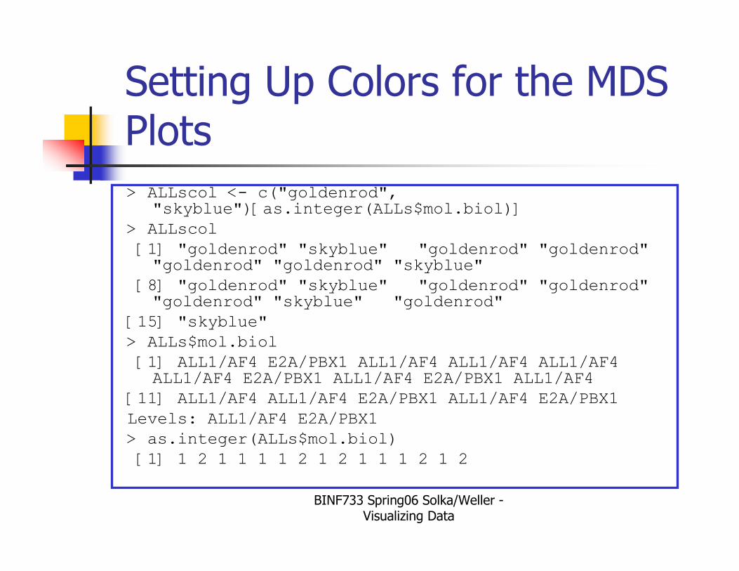
> ALLscol <- c("goldenrod", "skyblue")[as.integer(ALLs$mol.biol)]

> ALLscol

[1] "goldenrod" "skyblue" "goldenrod" "goldenrod" "goldenrod" "goldenrod" "skyblue"

[8] "goldenrod" "skyblue" "goldenrod" "goldenrod" "goldenrod" "skyblue" "goldenrod"

[15] "skyblue"

> ALLs$mol.biol

[1] ALL1/AF4 E2A/PBX1 ALL1/AF4 ALL1/AF4 ALL1/AF4ALL1/AF4 E2A/PBX1 ALL1/AF4 E2A/PBX1 ALL1/AF4

[11] ALL1/AF4 ALL1/AF4 E2A/PBX1 ALL1/AF4 E2A/PBX1

Levels: ALL1/AF4 E2A/PBX1

> as.integer(ALLs$mol.biol)

[1] 1 2 1 1 1 1 2 1 2 1 1 1 2 1 2


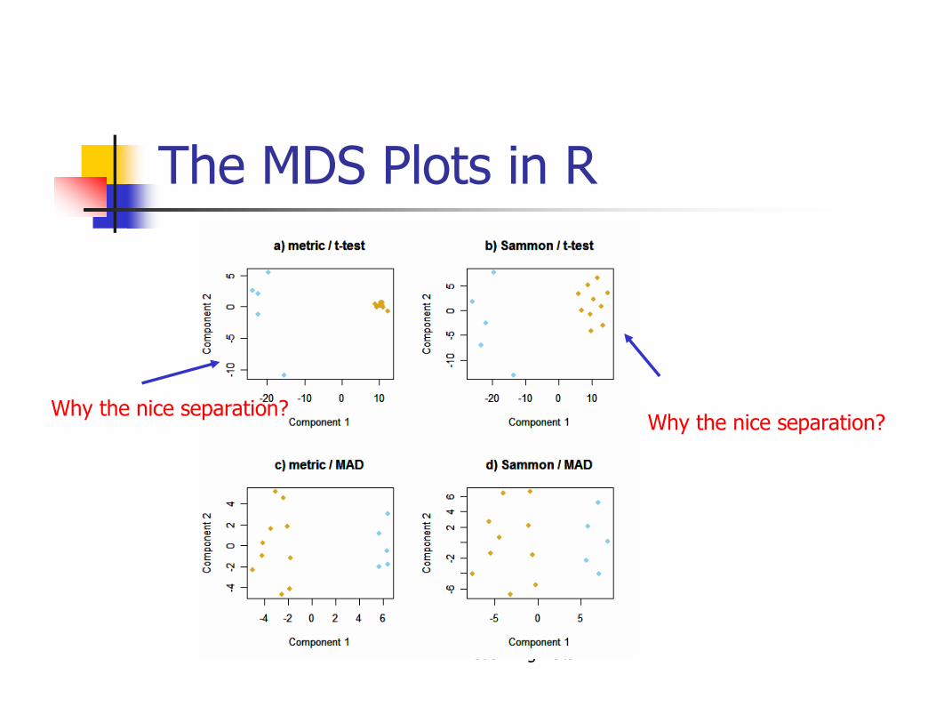
Creating the MDS Plots in R

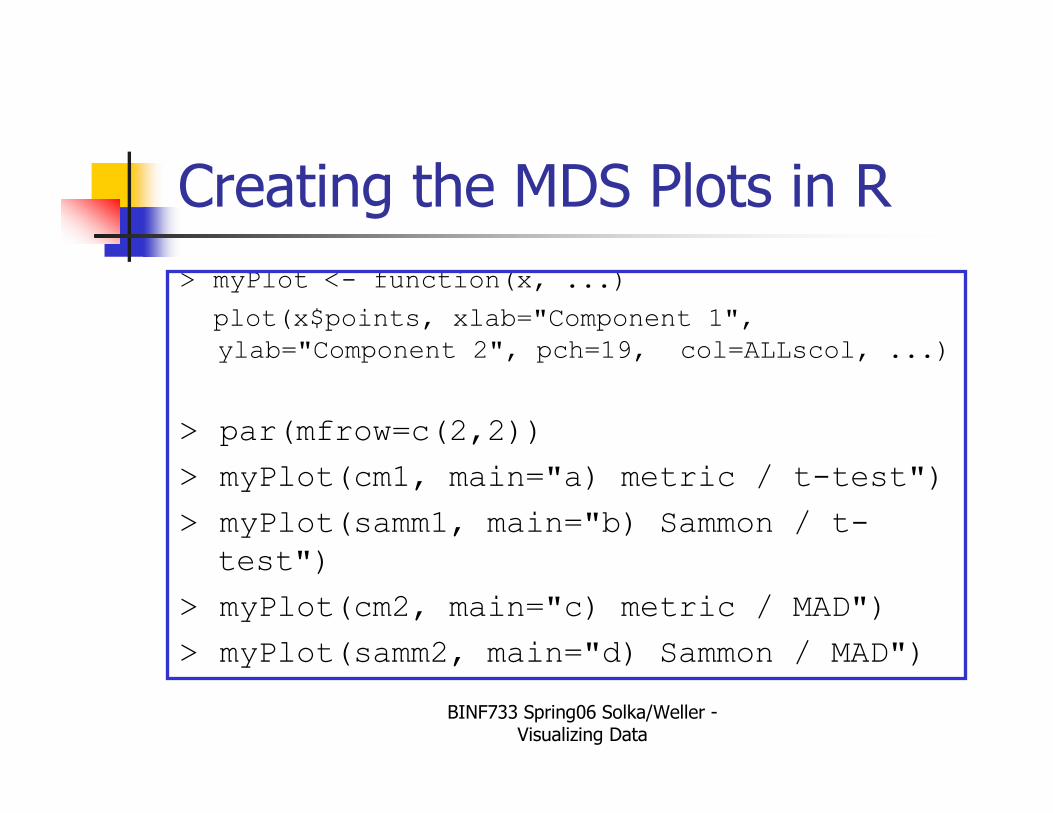
> myPlot <- function(x, ...)

plot(x$points, xlab="Component 1",

ylab="Component 2", pch=19, col=ALLscol, ...)

> par(mfrow=c(2,2))

> myPlot(cm1, main="a) metric / t-test")

> myPlot(samm1, main="b) Sammon / t-

test")

> myPlot(cm2, main="c) metric / MAD")

> myPlot(samm2, main="d) Sammon / MAD")


The MDS Plots in R

Why the nice separation?Why the nice separation?


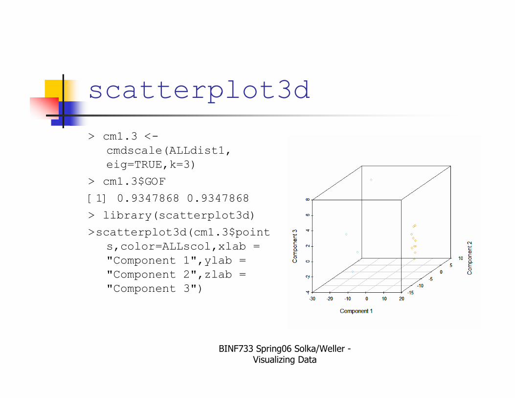
scatterplot3d

> cm1.3 <-

cmdscale(ALLdist1,

eig=TRUE,k=3)

> cm1.3$GOF

[1] 0.9347868 0.9347868

> library(scatterplot3d)

>scatterplot3d(cm1.3$point

s,color=ALLscol,xlab =

"Component 1",ylab =

"Component 2",zlab =

"Component 3")


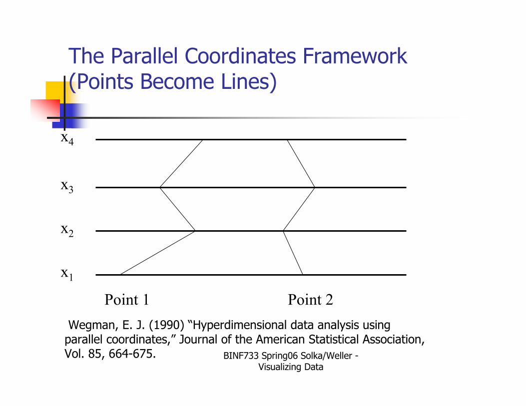
The Parallel Coordinates Framework(Points Become Lines)

x1

x2

x3

x4

Point 1 Point 2

Wegman, E. J. (1990) “Hyperdimensional data analysis using parallel coordinates,” Journal of the American Statistical Association, Vol. 85, 664-675.


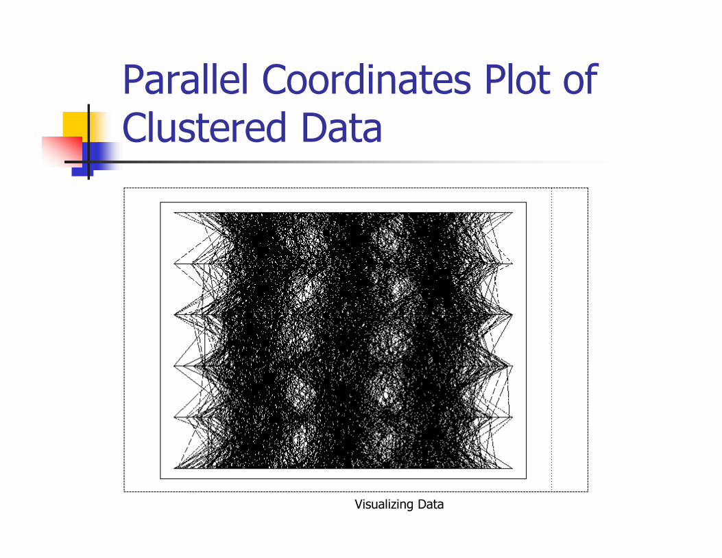
Parallel Coordinates Plot of Clustered Data


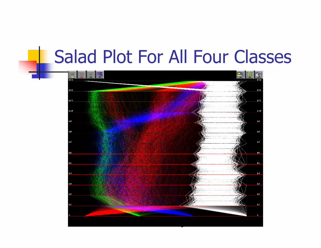
Salad Plot For All Four Classes


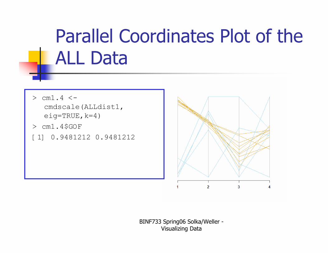
Parallel Coordinates Plot of the ALL Data

> cm1.4 <-

cmdscale(ALLdist1,

eig=TRUE,k=4)

> cm1.4$GOF

[1] 0.9481212 0.9481212


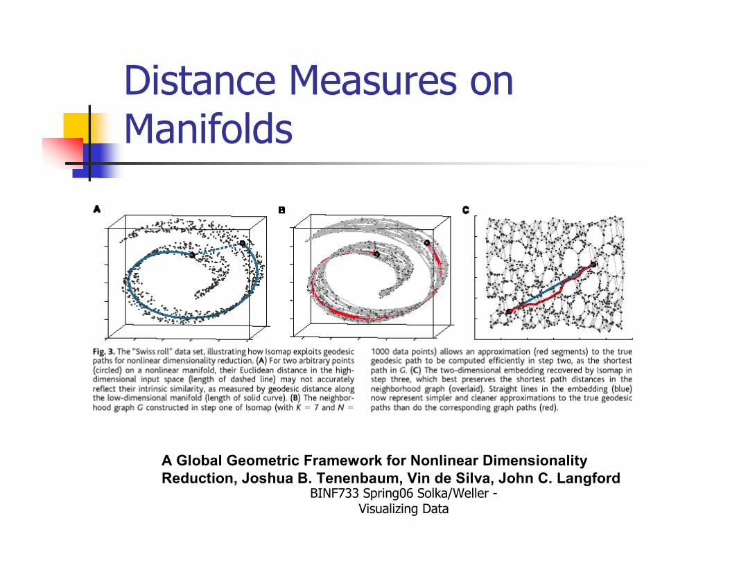
Distance Measures on Manifolds

A Global Geometric Framework for Nonlinear Dimensionality

Reduction, Joshua B. Tenenbaum, Vin de Silva, John C. Langford

The ISOMAP Algorithm

A Global Geometric Framework for Nonlinear Dimensionality

Reduction, Joshua B. Tenenbaum, Vin de Silva, John C. Langford


ISOMAP in Action

� Ref. Bioinformatics ISOMAP paper and snapshot some pictures.


Plotting Along Genomic Coordinates - I

� These tools relate gene expression to chromosomal location

� DNA

� Sense strand (Watson or + strand)

� Antisense strand (Crick or – strand)


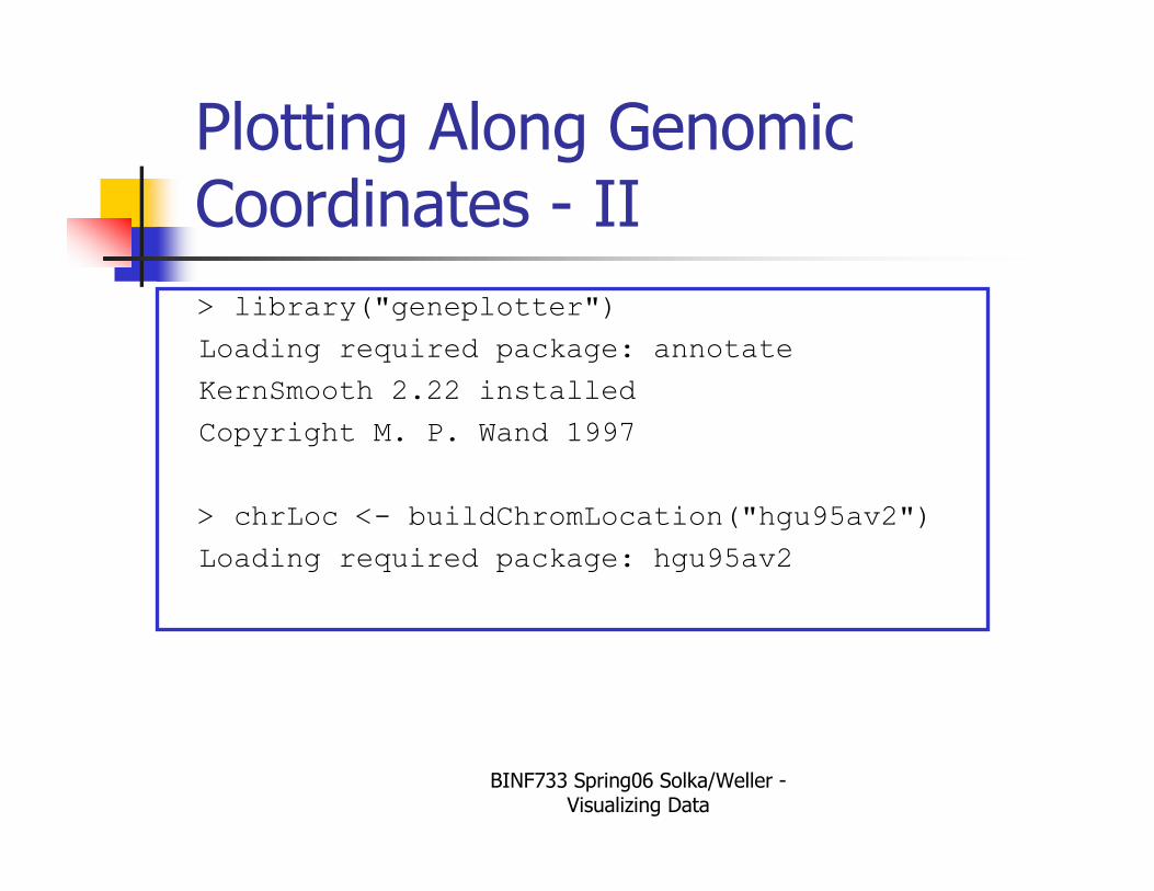
Plotting Along Genomic Coordinates - II

> library("geneplotter")

Loading required package: annotate

KernSmooth 2.22 installed

Copyright M. P. Wand 1997

> chrLoc <- buildChromLocation("hgu95av2")

Loading required package: hgu95av2


Plotting Along Genomic Coordinates - III

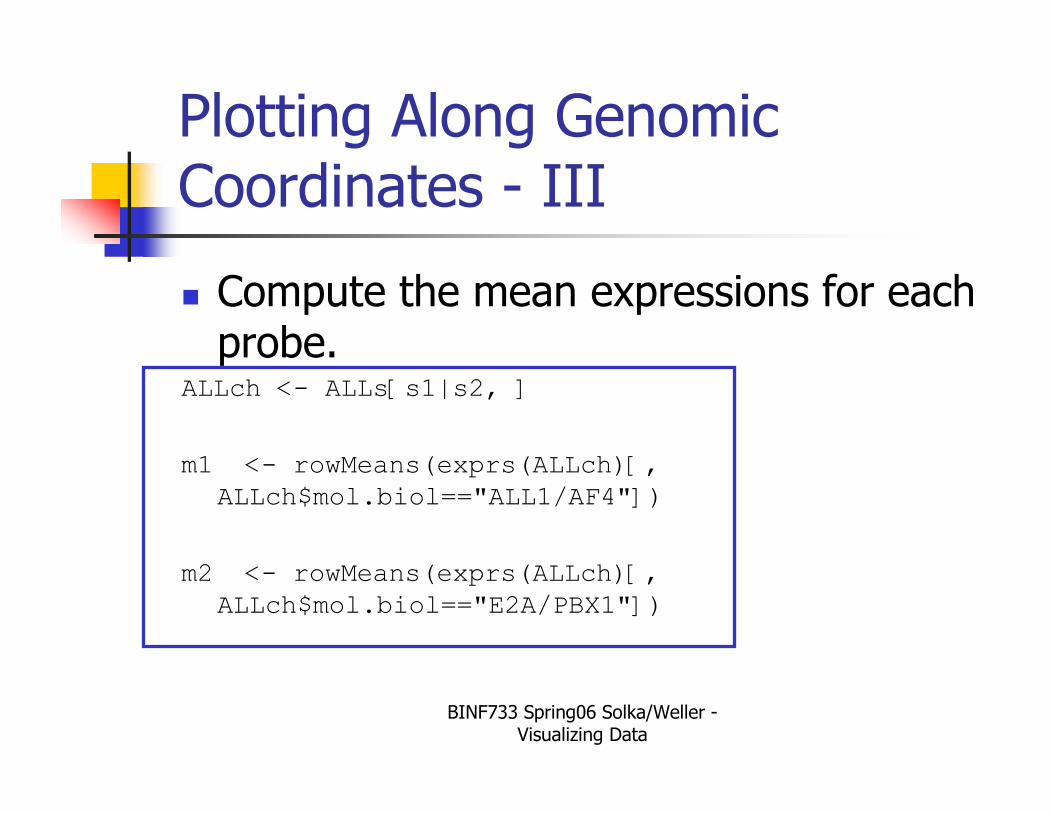
� Compute the mean expressions for each probe.

ALLch <- ALLs[s1|s2, ]

m1 <- rowMeans(exprs(ALLch)[,

ALLch$mol.biol=="ALL1/AF4"])

m2 <- rowMeans(exprs(ALLch)[,

ALLch$mol.biol=="E2A/PBX1"])


Plotting Along Genomic Coordinates - IV

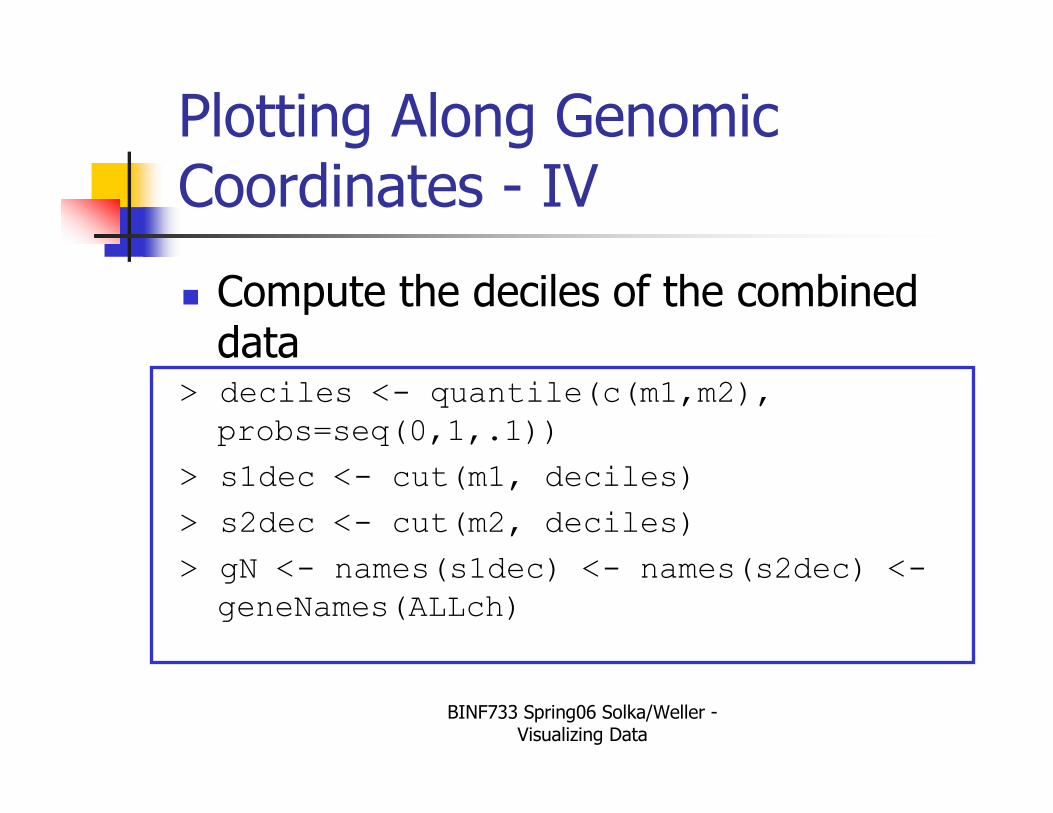
� Compute the deciles of the combined data

> deciles <- quantile(c(m1,m2),

probs=seq(0,1,.1))

> s1dec <- cut(m1, deciles)

> s2dec <- cut(m2, deciles)

> gN <- names(s1dec) <- names(s2dec) <-

geneNames(ALLch)


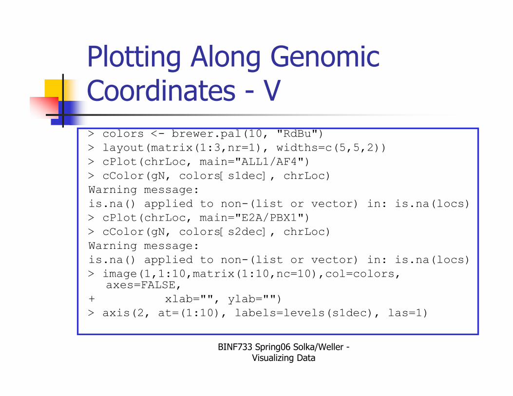
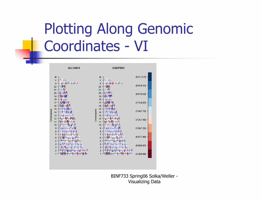
Plotting Along Genomic Coordinates - V

> colors <- brewer.pal(10, "RdBu")

> layout(matrix(1:3,nr=1), widths=c(5,5,2))

> cPlot(chrLoc, main="ALL1/AF4")

> cColor(gN, colors[s1dec], chrLoc)

Warning message:

is.na() applied to non-(list or vector) in: is.na(locs)

> cPlot(chrLoc, main="E2A/PBX1")

> cColor(gN, colors[s2dec], chrLoc)

Warning message:

is.na() applied to non-(list or vector) in: is.na(locs)

> image(1,1:10,matrix(1:10,nc=10),col=colors, axes=FALSE,

+ xlab="", ylab="")

> axis(2, at=(1:10), labels=levels(s1dec), las=1)


Plotting Along Genomic Coordinates - VI


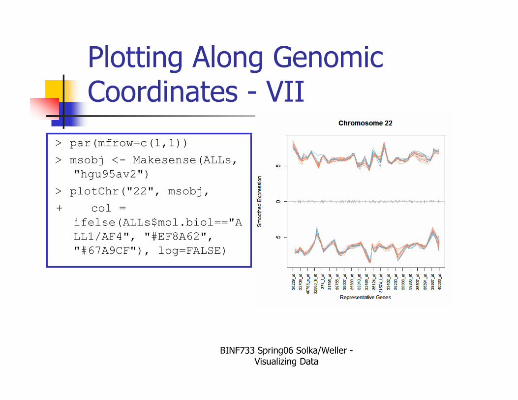
Plotting Along Genomic Coordinates - VII

> par(mfrow=c(1,1))

> msobj <- Makesense(ALLs,

"hgu95av2")

> plotChr("22", msobj,

+ col =

ifelse(ALLs$mol.biol=="A

LL1/AF4", "#EF8A62",

"#67A9CF"), log=FALSE)

Documents

BINF733s2006 VisualizingData solka - UB · W. S. Cleveland, Visualizing Data. Hobart Press, Summit, New Jersey, 1993. W. S. Cleveland. The Elements of Graphing Data (Revised).Hobart