Embed Size (px)
Citation preview
Binaural Sound Reproduction via
Distributed Loudspeaker Systems
Diplomarbeit
durchgeführt von
Martin TESCHL
Institut für Elektronische Musik
der Universität für Musik und darstellende Kunst Graz
durchgeführt am
Institute of Sound and Vibration Research
University of Southampton, UK
Betreuer:Prof. Philip A. NelsonTakashi TakeuchiProf. Robert Höldrich Graz, im Dezember 2000

Diese Diplomarbeit ist meinen Eltern, Franz und Maria Teschl, gewidmet.
This thesis is dedicated to my parents.
Abstract
The basic principle of binaural sound reproduction technique is to reconstruct the same soundpressures at a listener's eardrums that would have caused there by a real sound source to besimulated. Consequently, the listener cannot distinguish between the real sound source andthe generated virtual sound source. If a pair of loudspeakers is used, the appropriate earsignals are delivered to the listener by inverting the transmission paths between the twoloudspeakers and the two ears. This process, known as "crosstalk cancellation", can beconsidered as an inversion of a [2 × 2] matrix of transfer functions.Previous work undertaken in this area was concentrated on the use of a conventional stereoset-up where the loudspeakers span an angle of 60° as seen from the listener. As opposed to astereo set-up, by using two closely spaced loudspeakers, the performance had proven morerobust with respect to misalignment or movement of the listener's head. However, onedisadvantage of this approach is the source strengths required for the crosstalk cancellation atlow frequencies. In terms of matrix algebra, the crosstalk cancellation problem is said to be"ill-conditioned" at these frequencies.Based on a free-field model of the problem, it can be shown that ill-conditioning depends onfrequency and the loudspeaker span of the system, respectively. For instance, for a smallerspan the system inversion is ill-conditioned at low frequencies, whereas for larger sourcespans the conditioning is worse at higher frequencies. This connection resulted in the idea tovary the source span as a function of frequency in order to maintain the best possibleconditioning over the whole frequency range. A practical solution of this new approach is touse multiple pairs of loudspeakers for each frequency range with corresponding source spansin order to eventually cover the whole audible frequency range.This diploma thesis will discuss the potential for such an approach. Theory, practicalimplementation, and testing of such systems will be described in detail. Many soundlocalisation experiments were conducted in order to subjectively validate the system'sperformance. Results show a significant improvement, in particular with respect to azimuthlocalisation for virtual images well to the sides.

Zusammenfassung
Das Grundprinzip binauraler Schallwiedergabetechnik ist, denselben Schalldruck amTrommelfell eines Hörers zu rekonstruieren, der dort von einer realen Schallquelle verursachtwerden würde. Als Folge kann der Hörer nicht mehr zwischen der realen und der simulierten,virtuellen Schallquelle unterscheiden. Bei der Verwendung von zwei Lautsprechern, müssendie Übertragungsfunktionen zwischen den beiden Lautsprechern und den beiden Ohreninvertiert werden, um die entsprechenden Signale korrekt an die Ohren des Hörers zu liefern.Dieser Vorgang, der allgemein als Übersprechkompensation bezeichnet wird, kann als eineInversion einer [2 × 2] Matrix von Übertragungsfunktionen betrachtet werden.Frühere Arbeiten auf diesem Gebiet haben sich auf die Verwendung eines konventionellenStereo Systems konzentriert, wo die beiden Lautsprecher einen Winkel von 60° aufspannen.Im Vergleich dazu hat sich eine Anordnung der beiden Lautsprecher sehr nahe aneinander alsrobuster in Bezug auf Kopfbewegung des Hörers bzw. auf ungenaue Positionierungherausgestellt. Ein Nachteil dieser Methode ist jedoch, dass die Übersprechkompensationsehr hohe Lautsprechersignale im Niederfrequenzbereich erfordert. Inverse Probleme dieserArt werden in der Matrixalgebra als eine "schlecht gestellte Aufgabe" bezeichnet, oder mansagt, die Aufgabe ist "schlecht konditioniert".Anhand eines Freifeldmodells des Kompensationsproblems kann gezeigt werden, dassschlechte Konditionierung neben der Frequenz auch von der Geometrie derLautsprecheranordnung (vom aufgespannten Winkel) abhängig ist. So ist dieSysteminversion mit kleineren Winkeln im Niederfrequenzbereich schlecht konditioniert,wohingegen größere Aufspannwinkel schlechtere Konditionierung für hohe Frequenzenergeben. Dieser Zusammenhang hat zur Idee geführt, den Aufspannwinkel abhängig von derFrequenz zu variieren um so die bestmögliche Konditionierung über den gesamtenFrequenzbereich zu sichern. Eine praktische Lösung dafür ist die Verwendung mehrererLautsprecherpaare für verschiedene Frequenzbereiche, die jeweils unter entsprechendenWinkeln angeordnet werden um letztlich den gesamten hörbaren Frequenzbereichabzudecken.Diese Diplomarbeit diskutiert die generelle Machbarkeit und Möglichkeiten einer derartigenMethode. Die zugrundeliegende Theorie, die praktische Umsetzung sowie die Erprobungsolcher Systeme wird im Detail beschrieben. Resultate von umfassenden Schallokalisierungs-experimenten zeigen eindeutig signifikante Verbesserung, im speziellen hinsichtlich derAzimutlokalisierung für stark seitlich präsentierte virtuelle Schallquellen.
Acknowledgements:

First and foremost, I would like to thank Professor Philip Nelson and Mr. Takashi Takeuchi,
my supervisors at the ISVR in Southampton, for their constant encouragement, guidance,
enthusiasm, vital help, patience and kindness throughout the progress of this project. I would
also like to thank Professor Robert Höldrich, my supervisor in Graz, especially for the helpful
discussions concerning the data analysis of the subjective experiments.
I am most grateful to my parents who gave me all the wonderful opportunities in my life and
who always support me in everything I do.

Contents
CHAPTER 1 INTRODUCTION....................................................................................... 1
1.1 INTRODUCTION AND LITERATURE REVIEW..................................................................... 1
1.2 OBJECTIVES.................................................................................................................... 3
1.3 ORGANISATION OF THIS DOCUMENT ............................................................................... 6
CHAPTER 2 SPATIAL HEARING ................................................................................. 8
2.1 INTRODUCTION............................................................................................................... 8
2.2 HEAD-RELATED COORDINATE SYSTEMS ........................................................................ 9
2.3 INTERAURAL CUES....................................................................................................... 11
2.4 SPECTRAL CUES ........................................................................................................... 13
2.5 DISTANCE CUES ........................................................................................................... 15
2.6 DYNAMIC CUES............................................................................................................ 17
2.7 THE PRECEDENCE EFFECT............................................................................................ 18
2.8 LOCALISATION AND REVERBERATION.......................................................................... 19
2.9 HEAD-RELATED TRANSFER FUNCTIONS....................................................................... 22
CHAPTER 3 3D SOUND REPRODUCTION............................................................... 26
3.1 INTRODUCTION............................................................................................................. 26
3.2 BINAURAL SYNTHESIS OF VIRTUAL SOUND SOURCES.................................................. 27
3.3 HEADPHONE DISPLAYS ................................................................................................ 30
3.4 THEORY OF CROSSTALK CANCELLATION ..................................................................... 30
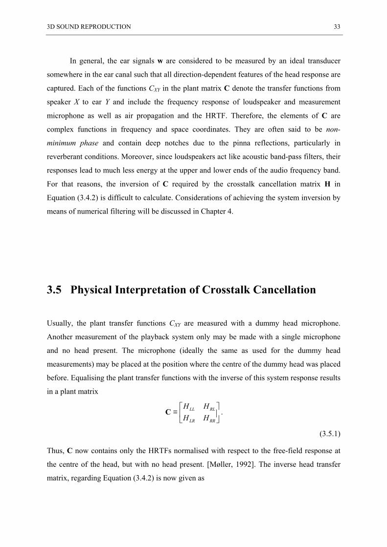
3.5 PHYSICAL INTERPRETATION OF CROSSTALK CANCELLATION....................................... 33
3.6 STEREO DIPOLE............................................................................................................ 35

CONTENTS II
CHAPTER 4 INVERSE FILTER DESIGN................................................................... 38
4.1 INTRODUCTION............................................................................................................. 38
4.2 EXACT INVERSION OF SINGLE CHANNEL SYSTEMS ...................................................... 39
4.3 OPTIMAL SINGLE CHANNEL INVERSION ....................................................................... 44
4.4 REGULARISATION......................................................................................................... 49
4.5 MULTI-CHANNEL SYSTEM INVERSION ......................................................................... 51
4.6 FAST DECONVOLUTION USING REGULARISATION......................................................... 53
4.7 ILL-CONDITIONING AND THE EFFECT OF REGULARISATION ........................................... 54
CHAPTER 5 OPTIMAL SOURCE DISTRIBUTION ................................................. 58
5.1 INTRODUCTION............................................................................................................. 58
5.2 FREE FIELD MODEL OF THE SYSTEM.............................................................................. 58
5.3 DYNAMIC RANGE LOSS................................................................................................ 61
5.4 ROBUSTNESS OF THE SYSTEM INVERSION .................................................................... 63
5.5 EFFECT OF REGULARISATION ....................................................................................... 64
5.6 PRINCIPLE OF THE “OSD” SYSTEM............................................................................... 65
5.7 PRACTICAL DISCRETE SYSTEM..................................................................................... 67
5.8 DESIGN CONSIDERATIONS............................................................................................ 69
5.9 EXAMPLES OF “OSD” SYSTEMS ................................................................................... 70
5.10 INVERSE FILTERING WHEN USING CROSS-OVER FILTERS ............................................... 73
CHAPTER 6 SYSTEM DESIGN.................................................................................... 77
6.1 INTRODUCTION............................................................................................................. 77
6.2 GENERAL SET-UP DESCRIPTION ................................................................................... 77
6.3 MEASUREMENTS OF THE PLANT MATRIX ..................................................................... 81
6.4 MEASUREMENT METHOD............................................................................................. 82
6.5 MEASUREMENT PROCEDURES ...................................................................................... 84
6.6 PROCESSING AND DATA REDUCTION............................................................................ 86
6.7 MEASUREMENT RESULTS ............................................................................................. 87

CONTENTS III
CHAPTER 7 SUBJECTIVE EXPERIMENTS ............................................................. 91
7.1 INTRODUCTION............................................................................................................. 91
7.2 EXPERIMENTAL SET-UP ................................................................................................ 91
7.3 PILOT STUDY - GENERAL IMPRESSION ......................................................................... 93
7.4 CHOICE OF TARGET LOCATIONS................................................................................... 95
7.5 PREPARATIONS OF TEST STIMULI ................................................................................. 97
7.6 LOCALISATION EXPERIMENT PROCEDURE.................................................................... 99
7.7 STATISTICAL ANALYSIS.............................................................................................. 101
CHAPTER 8 RESULTS AND DISCUSSION ............................................................. 105
8.1 INTRODUCTION........................................................................................................... 105
8.2 AZIMUTH LOCALISATION ........................................................................................... 105
8.3 ELEVATION LOCALISATION ........................................................................................ 109
8.4 ANGULAR ERROR STATISTIC...................................................................................... 113
8.5 FRONT-BACK REVERSALS.......................................................................................... 117
8.6 CONCLUDING REMARKS............................................................................................. 120
BIBLIOGRAPHY ............................................................................................................... 123
Chapter 1 Introduction
1.1 Introduction and Literature Review
Basically, any 3D sound reproduction system attempts to give a listener a sense of ”space”,
and hence must somehow make the listener believe that sound is coming from a position
where no real sound source exists in fact. This approach is usually referred to as virtual
source imaging.
A considerable part of current research into virtual source imaging systems relies
heavily on binaural technology. This technique can be considered as the art of ”fooling” the
human auditory mechanism for sound localization. It is based on the sensible engineering
principle that if a sound reproduction system is able to generate the same sound pressures at
the listener’s eardrums as would have been reproduced there by a real sound source, then the
listener should not be able to tell the difference between the virtual image and the real sound
source. In order to determine these binaural signals, or ”target” signals, it is necessary to
know how the listener’s torso (upper body), head and pinnae (outer ears) modify the
incoming sound waves according to a specific position of the sound source. This information
can be obtained by means of measurements on “dummy heads” or human subjects [Kleiner,
1978; Møller et al. 1997]. The results of such measurements are usually called Head-Related
Transfer Functions, or just HRTFs. Any synthetic binaural signal can be created by
convolving (filtering) a monophonic sound signal with the appropriate pair of HRTFs, a
procedure referred to as binaural synthesis.
In order to correctly deliver the binaural signal to a listener using transducers, the
signal must be equalized to compensate for the transmission paths from the transducers to the
INTRODUCTION 2
eardrums. In terms of control theory, these transmission paths are usually referred to as the
“plant”, which denotes the physical system to be controlled.
Headphones are often used for binaural audio because they ensure excellent channel
separation, they can isolate the listener from external sounds and room reverberation, and the
transmission paths from the transducers to the ears are easily equalized. An alternative to
headphones is the use of conventional stereo loudspeakers placed in front of the listener. In
this case, the transmission path equalization is accomplished by inverting the [2 × 2] matrix
of transfer functions between the two loudspeakers and the two ears. This procedure is called
crosstalk cancellation since it involves the acoustical cancellation of the unwanted crosstalk
from each speaker to the opposite ear. Usually, the term ”generalized” is added to
characterize crosstalk cancellation systems that account for the influence of the listener’s
head by allowing realistic HRTFs to be included. Thus, the purpose of generalized crosstalk
cancellation is to be able to produce a specified desired signal very accurately at one ear of
the listener, while nothing is heard at the other ear. Once this can be achieved, any pair of
binaural signals can be produced at the ears of a listener.
The technique of crosstalk cancellation was first introduced by Bauer [1961], and put
into practice by Schroeder and Atal [1963; Atal et al., 1966]. Later, it was subjectively
verified by Damaske [1971] and Schroeder [1975] with good results even for phantom
images positioned outside the angle spanned by the loudspeakers. The method, using analog
techniques, was based on a free-field model that did not account for the presence of the
listener in the sound field. Since then, more sophisticated methods, some based on digital
signal processing techniques, have been developed for generalized crosstalk cancellation,
such as by Cooper and Bauck [1989]; Bauck and Cooper [1996], Kirkeby et al. [1996a],
Nelson et al. [1992, 1995], Nelson and Orduña-Bustamente [1996], Griesinger [1989], and
Møller [1989].
With a few notable exceptions [Bauck and Cooper, 1996; Heegaard, 1992], most
researchers have concentrated on systems using the traditional stereo loudspeaker
arrangements spanning an angle of typically 60 degrees as seen by the listener. A
fundamental problem that one faces when using relatively widely spaced loudspeakers is that
the listener’s ears are required to be within a rather small region (”equalization zone”) which
is under the control of the system. Misalignment of the head results in a change of the HRTFs
and thus in an inaccurate synthesis of the binaural signals. Consequently, the directional
INTRODUCTION 3
information associated with the acoustic signals is inaccurately reproduced. In addition, the
digital signal processing tends to give the reproduced sound an unpleasant “coloration”.
However, a system using two closely spaced loudspeakers turned out to be
surprisingly robust with respect to head movement [Takeuchi et al., 1997], and it also avoids
coloration of the reproduced sound. The size of the equalization zone around the listener’s
head is increased significantly without any noticeable reduction in performance. Kirkeby et
al. [1996b; 1997] use the term “Stereo Dipole” to describe such a virtual source imaging
system since the inputs to the two closely spaced loudspeakers are close to being exactly out
of phase over a wide frequency range [Kirkeby and Nelson, 1997]. Consequently, they
reproduce a sound field very similar to that generated by a point dipole source. Strictly
speaking, the reproduced field rather approximates that field generated by a combination of a
point dipole and a point monopole source at the same position [Nelson et al., 1997; Bauck
and Cooper, 1996]. Thus, it would be more accurate to use the term “stereo monopole-
dipole”.
1.2 Objectives
In practice, crosstalk-cancelling systems suffer from a variety of problems apart from the fact
that they are fairly sensitive to the position of the listener’s head. First of all is that the multi-
channel system inversion involved with crosstalk-cancellation requires amplification of the
signal at certain frequencies and attenuation of the signal at other frequencies. The maximum
required amplification yields the maximum output signal of the system, which must be within
the range of the overall system in order to avoid clipping of the signals. Thus, the maximum
amplification due to the system inversion directly results in loss of dynamic range.
The stability or robustness of the system inversion is another important problem. The
electro-acoustic transfer functions of the transmission path between loudspeakers and the
listener’s ears show very small magnitudes at certain frequencies. These frequencies are
usually referred as being “ill-conditioned” because the inversion of their magnitudes results
in very high values [Wilkinson, 1965]. Thus, a small change (a small error) in the transfer
INTRODUCTION 4
function (e.g. due to a slight movement of the listener) causes a large change in the solution
for the inverse filter around ill-conditioned frequencies. In order to avoid this,
“regularisation” is often used in the design of practical filters for multi-channel system
inversion [Press et al., 1992; Kirkeby et al., 1996a]. In principle, the technique of
regularisation allows to reduce both dynamic range loss caused by the system inversion, and
sensitivity to small changes around ill-conditioned frequencies. This is done by means of
penalising the excess amplification due to the inversion, but this in turn results in poor
control performance around ill-conditioned frequencies. In other words, regularisation is a
matter of finding an appropriate trade-off between allowed dynamic range loss, limiting large
output magnitudes around ill-conditioned frequencies, and obtaining a desired control
performance in terms of crosstalk cancellation.
In general, the problems of dynamic range loss and ill-conditioning depend on
frequency and on the positions of the reproduction loudspeakers relative to the ears. For
instance, as the loudspeaker span is reduced, it is much harder to achieve efficient crosstalk
cancellation at low frequencies, and, in addition, an increasing amount of low-frequency
energy is required in order to create a virtual source image at a position well outside the
angles spanned by the two loudspeakers [Kirkeby et al., 1997; 1998].
More specified investigations show that a small loudspeaker span creates a system
that is “well-behaving” within a wide region in the middle-band frequencies, whereas a large
loudspeaker span works better at low frequencies [Takeuchi and Nelson, 2000a; 2000b]. In
fact, these results represent the main feature as well as the main drawback of the “Stereo-
Dipole” system. Though, using closely spaced loudspeakers greatly widens the equalisation
zone in the middle-band frequencies, it compromises the performance at low frequencies
considerably. Without any precautions, the inverse filters tend to excessively amplify the ill-
conditioned low frequencies, which likely leads to saturation of the audio amplifiers and/or
damage of the loudspeakers.
However, if one were able to continuously vary the loudspeaker span as a function of
frequency, this problems could be ideally solved. A practical solution for this is to divide the
audible frequency range into two or more bands, and hence “discretise” the loudspeaker span.
The low frequency band is reproduced through widely spaced loudspeakers while the
loudspeakers for the high frequency band are spaced closer together. Although this
arrangement uses four or more loudspeakers, it still has to be considered as a two-channel
INTRODUCTION 5
loudspeaker system. Following this idea, Takeuchi and Nelson [2000a; 2000b] accomplished
extensive investigations, based on a free-field model of the problem, in order to find optimal
solutions of how to dicretise the audible frequency range and how to distribute the
loudspeakers. Eventually, these investigations resulted in the proposal of a new virtual
acoustic system, referred to as “Optimal Source Distribution” or “OSD” system. Thereby,
the word “optimal” indicates that the system has to be designed to ensure as well behaviour
of the system as possible over a frequency range that is as wide as possible.
The main objective of the present work is to put such a system into practice and
investigate its performance. Cross-over filters (low pass, high pass, or band pass) are used in
order to distribute the signals of the appropriate frequency range to the appropriate pair of
driver units. Other than for the ideal case of theoretical simulations, there are transition
regions around the cross-over frequencies where multiple pairs of loudspeakers are
contributing significantly to the synthesis of the reproduced binaural signals. This is obvious
because an ideal cross-over filter which gives a rectangular window in the frequency domain
cannot be realised in practice. Therefore, it is important to ensure the transition regions of the
cross-over filters are also within the “well-behaving” range of the applied principle.
If the matrix of transmission paths (the plant matrix) is measured when including the
cross-over network, it contains the responses of the cross-over network as well as the
interaction between different pairs of loudspeakers. Designing the inverse filter matrix from
this plant matrix is obviously the most straightforward among other options, since it
automatically compensates for the cross-over network. Alternatively, one can design inverse
filter matrices for plants of each pair of driver units separately. It is also possible to obtain the
plant matrix by measuring the transmission paths for each single transducer to the ears. In
that case, the system is underdetermined and the solution of the inverse filter matrix
distributes the signals to the different drivers such that “least effort” (i.e., the smallest
output) is required [Takeuchi and Nelson, 2000a, 2000b]. Omitting the cross-over filters
yields to a conventional multi-channel system, contrary to the “OSD” system which is a
multi-way system.
In any case, the cross-over filters can be passive, active, or digital filters. Obviously,
if they are digital filters, they can also be included in the same filters which implement the
system inversion.
INTRODUCTION 6
The aim of the present work is to investigate the technical feasibility of those various
options, and, as far as possible, to evaluate their advantages and disadvantages. The
performance in terms of accuracy of the inverse filtering, gain of dynamic range and crosstalk
cancellation is examined by means of physical measurements on the investigated systems.
Potential improvement of these parameters would eventually result in accurate virtual source
imaging, good signal-to-noise ratio, and sound quality as a general impression. The
subjective performance parameters are evaluated by means of extensive sound localisation
experiments. The project has been undertaken by the author at the Institute of Sound and
Vibration Research (ISVR), University of Southampton, in the time between 1st of March and
31st of August 2000.
1.3 Organisation of this document
The present degree dissertation has 8 chapters. The first following chapters after this
introduction will review two important topics relevant to this work. Chapter 2 discusses the
human mechanism of sound localisation, and spatial hearing, respectively. In Chapter 3, a
general discussion of 3D sound reproduction is addressed, particularly with regard to binaural
techniques for virtual sound source imaging. Hereby, the basic idea related to the theory of
crosstalk cancellation will be especially emphasised as well as particular features of the
“Stereo Dipole” system. Digital signal processing theory concerning the practical design of
digital inverse filters for crosstalk cancellation will be considered in Chapter 4. The problems
of ill-conditioning and loss of dynamic range will be discussed in detail. In Chapter 5, the
“OSD” system will be proposed as a possible solution of the mentioned problems. The basic
ideas behind this method will be outlined based on the papers by Takeuchi and Nelson
[2000a, 2000b]. Chapter 6 comprises a comprehensive discussion of the practical
implementation of the systems, as well as a description of the experimental set-up and
measurement procedures. Considerations about the subjective evaluation of the system are
addressed in Chapter 7. In particular, the procedure of sound localisation experiments are
explained. Finally, Chapter 8 concludes with a summary and discussion of the results of this

INTRODUCTION 7
study. Areas of future work are suggested.
Chapter 2 Spatial Hearing
2.1 Introduction
As indicated in the first chapter, typical applications of 3D sound systems complement,
modify, or replace sound attributes that occur in natural listening situations in order to obtain
control on one’s spatial perception. This control can not be achieved based on physical
attributes only. Psychoacoustic considerations of the human sound localisation also play
important roles in analysing, designing, and testing 3D sound systems. In order to manipulate
a listener’s spatial auditory perception, a thorough understanding of the psychoacoustical
phenomena occurring in natural spatial hearing is essential. By modifying the physical
parameters associated with those phenomena, the control goal may be achieved.
The important cues used by the human auditory system to localise sound sources in
space, are identified by psychoacoustic experiments [Blauert, 1997]. It is widely believed that
localisation of sources in the horizontal plane (azimuth localisation)1 is due to the differences
between the sound waves received at each ear (interaural differences). Localisation of sound
sources not in the horizontal plane (elevation localisation) is strongly influenced by spectral
cues due to the acoustic filtering of short wavelength sound waves. Human listeners are also
capable of estimating the sound source distance in addition to azimuth and elevation angles.
Interaural, spectral, and distance cues are discussed in Sections 2.3, 2.4, and 2.5, respectively.
When the above mentioned cues are ambiguous, humans usually move their heads
(some animals move their ears), so that more (or less) interaural and spectral cues are
1 See Figure 2.2.1 for the definition of these terms.
SPATIAL HEARING 9
introduced, making the localisation task easier. These dynamic cues are addressed in Section
2.6.
Room reverberation degrades human localisation performance, since the direction of
a reflected sound may be confused with the direction of the sound coming directly from the
source. However, thanks to the precedence effect, human listeners are still able to localise
sounds in reverberant environments. The precedence effect as well as physical and perceptual
aspects of room reverberation are discussed in Sections 2.7 and 2.8, respectively.
All physical parameters associated with the localisation cues that occur in natural
listening situations are embedded in the pair of acoustic transmissions from the source to
each of the listener’s eardrums. As mentioned in Chapter 1, these acoustic transmissions are
usually referred to as the Head-Related Transfer Function (HRTF) pair, and can be measured
and stored in the form of digital filters. The basic principle of modern 3D sound systems
based on binaural technology [Begault, 1994; Duda, 1996; Gardner, 1997; Wightman and
Kistler, 1989a] is to make use of this HRTF information in order to eventually control a
listener’s spatial perception. A thorough discussion of the physical properties of HRTFs
follows in Section 2.9.
2.2 Head-related Coordinate Systems
References to position in connection with spatial hearing are usually made in terms of a head-
related system of coordinates [Blauert, 1997]. This system is practically constant relative to
the position of the listener’s head and hence relative to the position of the ears. In the
following discussion throughout this document, the systems shown in Figure 2.2.1 will be
assumed. Both systems are chosen so that the origin is at the centre point between the
listener’s ears (the interaural axis). The +x-axis passes through the right ear, the +y-axis
points straight ahead, and the +z-axis is vertical. This defines the three standard planes, the xy
or horizontal plane, the xz or frontal plane, and the yz denotes the median plane.
Obviously, the horizontal plane defines up/down separation, the frontal plane defines
front/back separation, and the median plane defines right/left separation.
SPATIAL HEARING 10
Spherical coordinate systems are used here since the human head is approximately
spherical. Hereby the standard coordinates are the azimuth angle ϕ, the elevation angle δ, and
the range r. Unfortunately, these coordinates can be defined in different ways.
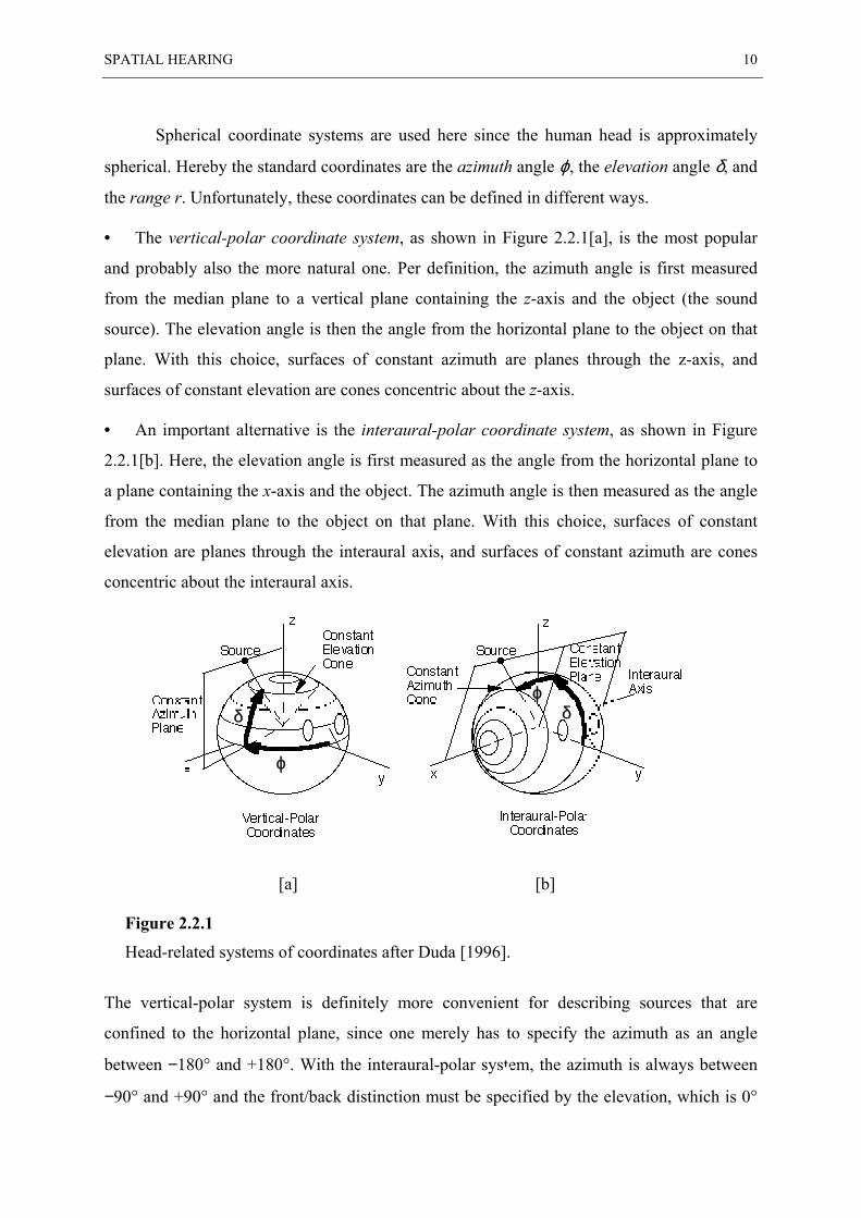
• The vertical-polar coordinate system, as shown in Figure 2.2.1[a], is the most popular
and probably also the more natural one. Per definition, the azimuth angle is first measured
from the median plane to a vertical plane containing the z-axis and the object (the sound
source). The elevation angle is then the angle from the horizontal plane to the object on that
plane. With this choice, surfaces of constant azimuth are planes through the z-axis, and
surfaces of constant elevation are cones concentric about the z-axis.
• An important alternative is the interaural-polar coordinate system, as shown in Figure
2.2.1[b]. Here, the elevation angle is first measured as the angle from the horizontal plane to
a plane containing the x-axis and the object. The azimuth angle is then measured as the angle
from the median plane to the object on that plane. With this choice, surfaces of constant
elevation are planes through the interaural axis, and surfaces of constant azimuth are cones
concentric about the interaural axis.
[a] [b]
Figure 2.2.1
Head-related systems of coordinates after Duda [1996].
The vertical-polar system is definitely more convenient for describing sources that are
confined to the horizontal plane, since one merely has to specify the azimuth as an angle
between −180° and +180°. With the interaural-polar system, the azimuth is always between
−90° and +90° and the front/back distinction must be specified by the elevation, which is 0°
ϕ
δϕ
δ
SPATIAL HEARING 11
for sources in the front horizontal plane, and ±180° for sources in the back. Even though this
may appear a bit clumsy, the interaural-polar system makes it significantly simpler to express
interaural differences at all elevations.
When using an interaural-polar coordinate system and by holding the azimuth constant, a
constant value for the Interaural Time Difference (ITD) is achieved. Thus, there is a simple
one-to-one correspondence between the ITD and the cone of constant azimuth, which is
usually called the "cone of confusion". This is not the case for the vertical-polar system. A
detailed description of these terms is given in the following Section 2.3. Depending on
whether azimuth or elevation was considered at a time, both coordinate systems were applied
for subjective experiments and the analysis of the results, as discussed in Chapter 7 and
Chapter 8, respectively.
2.3 Interaural Cues
In natural listening situations, the difference between sound waves received at the listener’s
left and right ears is an important cue used by the human auditory system to estimate the
sound source position in space. These difference cues, referred to as interaural or binaural
cues are best explained using the far field anechoic listening situation shown in Figure 2.3.1.
A sound signal emitted from a source S located in the horizontal plane at azimuth angle ϕ and
distance r from the centre of the listener’s head travels to the listener’s right (ipsilateral) and
left (contralateral)1 ears through path SR and SL, respectively. Since SR in this example is
shorter than SL, a sound wave reaches the right ear before the left ear. This difference in
arrival time is referred to as the Interaural Time Difference (ITD). Assuming a plane wave,
the ITD as a function of the azimuth angle ϕ is given by
( )ϕϕ sin+=caITD , −90° ≤ ϕ ≤ ϕ + 90°.
(2.3.1)
1 The term ipsilateral refers to the ear which is closer to the sound source, whereas the term contralateral
indicates the ear at the further distance to the sound source.
SPATIAL HEARING 12
The ITD is zero when the source is at azimuth zero (that is in the median plane), and is a
maximum at azimuth ±90°. This represents a difference of arrival time of about 0,7 ms for a
typical-size human head [Blauert, 1997]. ITD represents a powerful and dominating cue at
frequencies below about 1.5 kHz. At higher frequencies, the ITD represents an ambiguous
cue since it corresponds to a shift of many cycles of the incident sound wave. For complex
sound waves, the ITD of the envelope at high frequencies, which is referred to as the
Interaural Envelope Difference (IED), is perceived.
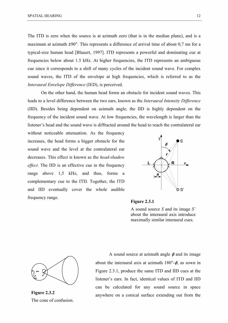
On the other hand, the human head forms an obstacle for incident sound waves. This
leads to a level difference between the two ears, known as the Interaural Intensity Difference
(IID). Besides being dependent on azimuth angle, the IID is highly dependent on the
frequency of the incident sound wave. At low frequencies, the wavelength is larger than the
listener’s head and the sound wave is diffracted around the head to reach the contralateral ear
without noticeable attenuation. As the frequency
increases, the head forms a bigger obstacle for the
sound wave and the level at the contralateral ear
decreases. This effect is known as the head-shadow
effect. The IID is an effective cue in the frequency
range above 1,5 kHz, and thus, forms a
complementary cue to the ITD. Together, the ITD
and IID eventually cover the whole audible
frequency range.
A sound source at azimuth angle ϕ and its image
about the interaural axis at azimuth 180°-ϕ, as sown in
Figure 2.3.1, produce the same ITD and IID cues at the
listener’s ears. In fact, identical values of ITD and IID
can be calculated for any sound source in space
anywhere on a conical surface extending out from the
S’
a
r
ϕS
y
xRL
Figure 2.3.1
A sound source S and its image S’about the interaural axis introducemaximally similar interaural cues.
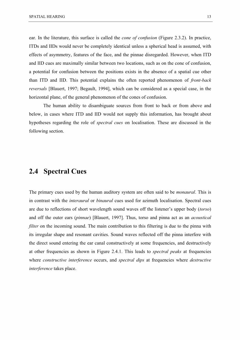
Figure 2.3.2
The cone of confusion.
SPATIAL HEARING 13
ear. In the literature, this surface is called the cone of confusion (Figure 2.3.2). In practice,
ITDs and IIDs would never be completely identical unless a spherical head is assumed, with
effects of asymmetry, features of the face, and the pinnae disregarded. However, when ITD
and IID cues are maximally similar between two locations, such as on the cone of confusion,
a potential for confusion between the positions exists in the absence of a spatial cue other
than ITD and IID. This potential explains the often reported phenomenon of front-back
reversals [Blauert, 1997; Begault, 1994], which can be considered as a special case, in the
horizontal plane, of the general phenomenon of the cones of confusion.
The human ability to disambiguate sources from front to back or from above and
below, in cases where ITD and IID would not supply this information, has brought about
hypotheses regarding the role of spectral cues on localisation. These are discussed in the
following section.
2.4 Spectral Cues
The primary cues used by the human auditory system are often said to be monaural. This is
in contrast with the interaural or binaural cues used for azimuth localisation. Spectral cues
are due to reflections of short wavelength sound waves off the listener’s upper body (torso)
and off the outer ears (pinnae) [Blauert, 1997]. Thus, torso and pinna act as an acoustical
filter on the incoming sound. The main contribution to this filtering is due to the pinna with
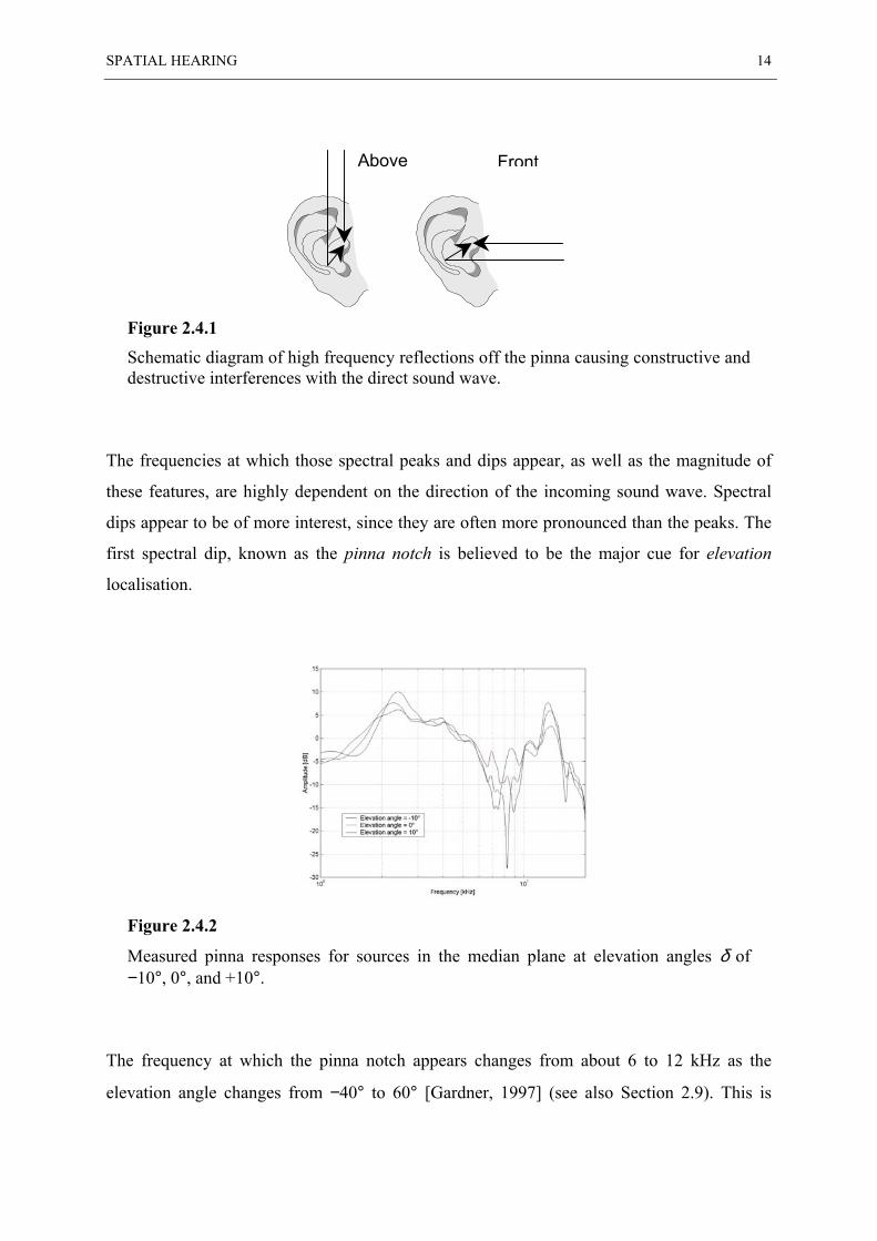
its irregular shape and resonant cavities. Sound waves reflected off the pinna interfere with
the direct sound entering the ear canal constructively at some frequencies, and destructively
at other frequencies as shown in Figure 2.4.1. This leads to spectral peaks at frequencies
where constructive interference occurs, and spectral dips at frequencies where destructive
interference takes place.
SPATIAL HEARING 14
Figure 2.4.1
Schematic diagram of high frequency reflections off the pinna causing constructive anddestructive interferences with the direct sound wave.
The frequencies at which those spectral peaks and dips appear, as well as the magnitude of
these features, are highly dependent on the direction of the incoming sound wave. Spectral
dips appear to be of more interest, since they are often more pronounced than the peaks. The
first spectral dip, known as the pinna notch is believed to be the major cue for elevation
localisation.
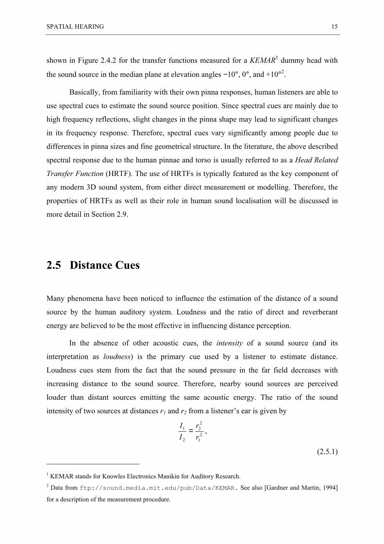
Figure 2.4.2
Measured pinna responses for sources in the median plane at elevation angles δ of−10°, 0°, and +10°.
The frequency at which the pinna notch appears changes from about 6 to 12 kHz as the
elevation angle changes from −40° to 60° [Gardner, 1997] (see also Section 2.9). This is
Above Front
SPATIAL HEARING 15
shown in Figure 2.4.2 for the transfer functions measured for a KEMAR1 dummy head with
the sound source in the median plane at elevation angles −10°, 0°, and +10°2.
Basically, from familiarity with their own pinna responses, human listeners are able to
use spectral cues to estimate the sound source position. Since spectral cues are mainly due to
high frequency reflections, slight changes in the pinna shape may lead to significant changes
in its frequency response. Therefore, spectral cues vary significantly among people due to
differences in pinna sizes and fine geometrical structure. In the literature, the above described
spectral response due to the human pinnae and torso is usually referred to as a Head Related
Transfer Function (HRTF). The use of HRTFs is typically featured as the key component of
any modern 3D sound system, from either direct measurement or modelling. Therefore, the
properties of HRTFs as well as their role in human sound localisation will be discussed in
more detail in Section 2.9.
2.5 Distance Cues
Many phenomena have been noticed to influence the estimation of the distance of a sound
source by the human auditory system. Loudness and the ratio of direct and reverberant
energy are believed to be the most effective in influencing distance perception.
In the absence of other acoustic cues, the intensity of a sound source (and its
interpretation as loudness) is the primary cue used by a listener to estimate distance.
Loudness cues stem from the fact that the sound pressure in the far field decreases with
increasing distance to the sound source. Therefore, nearby sound sources are perceived
louder than distant sources emitting the same acoustic energy. The ratio of the sound
intensity of two sources at distances r1 and r2 from a listener’s ear is given by
21
22
2
1
rr
II
= ,
(2.5.1) 1 KEMAR stands for Knowles Electronics Manikin for Auditory Research.2 Data from ftp://sound.media.mit.edu/pub/Data/KEMAR. See also [Gardner and Martin, 1994]
for a description of the measurement procedure.
SPATIAL HEARING 16
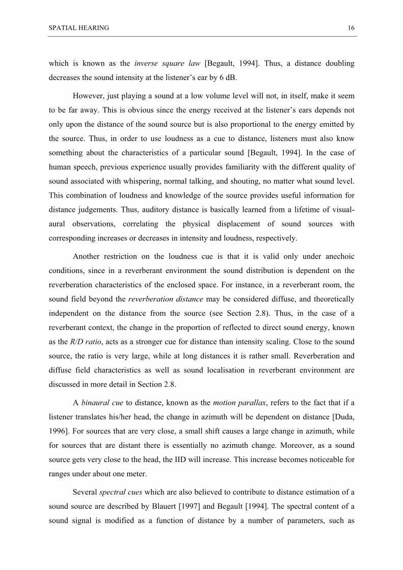
which is known as the inverse square law [Begault, 1994]. Thus, a distance doubling
decreases the sound intensity at the listener’s ear by 6 dB.
However, just playing a sound at a low volume level will not, in itself, make it seem
to be far away. This is obvious since the energy received at the listener’s ears depends not
only upon the distance of the sound source but is also proportional to the energy emitted by
the source. Thus, in order to use loudness as a cue to distance, listeners must also know
something about the characteristics of a particular sound [Begault, 1994]. In the case of
human speech, previous experience usually provides familiarity with the different quality of
sound associated with whispering, normal talking, and shouting, no matter what sound level.
This combination of loudness and knowledge of the source provides useful information for
distance judgements. Thus, auditory distance is basically learned from a lifetime of visual-
aural observations, correlating the physical displacement of sound sources with
corresponding increases or decreases in intensity and loudness, respectively.
Another restriction on the loudness cue is that it is valid only under anechoic
conditions, since in a reverberant environment the sound distribution is dependent on the
reverberation characteristics of the enclosed space. For instance, in a reverberant room, the
sound field beyond the reverberation distance may be considered diffuse, and theoretically
independent on the distance from the source (see Section 2.8). Thus, in the case of a
reverberant context, the change in the proportion of reflected to direct sound energy, known
as the R/D ratio, acts as a stronger cue for distance than intensity scaling. Close to the sound
source, the ratio is very large, while at long distances it is rather small. Reverberation and
diffuse field characteristics as well as sound localisation in reverberant environment are
discussed in more detail in Section 2.8.
A binaural cue to distance, known as the motion parallax, refers to the fact that if a
listener translates his/her head, the change in azimuth will be dependent on distance [Duda,
1996]. For sources that are very close, a small shift causes a large change in azimuth, while
for sources that are distant there is essentially no azimuth change. Moreover, as a sound
source gets very close to the head, the IID will increase. This increase becomes noticeable for
ranges under about one meter.
Several spectral cues which are also believed to contribute to distance estimation of a
sound source are described by Blauert [1997] and Begault [1994]. The spectral content of a
sound signal is modified as a function of distance by a number of parameters, such as
SPATIAL HEARING 17
atmospheric conditions, molecular absorption of the air, the curvature of the wavefront, air
humidity and temperature. At large distances in the environment outdoors, even the wind
profiles, ground cover, and barriers such as buildings give contribution. However, from a
psychoacoustic point of view, all these cues are relatively weak, compared to loudness,
familiarity, and reverberation cues.
2.6 Dynamic Cues
In ambiguous listening situations where interaural and spectral cues produce insufficient
information to localise the sound source, humans tend to turn their heads in order to minimise
(or maximise) the interaural differences; i.e., use the head as a sort of ”pointer” to resolve
ambiguity.
Ambiguous interaural cues are introduced at the listener’ ears due to the cone of
confusion phenomenon. A sound source at a certain azimuth angle ϕ to the right of the
listener in the horizontal plane introduces maximally similar interaural cues as a source at
azimuth angle 180°-ϕ as mentioned in Section 2.3. A human listener would resolve the
ambiguous interaural cues by turning his/her head to the right, since the ambiguous cues still
suggest that the source is at the listener’s right. After turning right, if the interaural cues are
minimised, the listener would decide that the source is in the front, otherwise if it is
maximised, the decision would be that the source is at the back. In general, listeners
apparently integrate some combination of the changes in ITD, IID, and movement of spectral
notches and peaks that occur with head movement over time, and subsequently use this
information to disambiguate, for instance, front imagery from rear imagery.
Although head movements improve the localisation performance in natural hearing,
they give rise to great difficulties to synthetic 3D sound systems. Unlike natural spatial
hearing, the integration of cues derived from head movement with both stereo loudspeakers
and headphones will provide false information for localising a virtual source. With
loudspeakers, a distortion of spatial imagery will occur when the head is turned to face the
virtual sound source, since the processing to create the illusion depends on a known
SPATIAL HEARING 18
orientation of the listener. With headphones, the head movement has no effect on localisation
of the sound, a situation that does not correspond to actual circumstances.
Just as moving the head causes dynamic changes for a fixed source, a moving source
will cause dynamic changes for a fixed head. One of the main cues for a moving source is the
Doppler shift, which denotes the change in pitch associated with source movement (e.g., a jet
plane passing overhead).
Cognitive cues are a large part of the sensation of motion. A monaural speaker, for
example, can give the sensation of a speeding automobile on a racetrack, through the
transmission of multiple, associative cues from experience.
2.7 The Precedence Effect
Natural sound localisation is affected by the above mentioned cues as well as by numerous
other psychoacoustical phenomena. One of those phenomena, the precedence effect, that is
directly related to localisation in reverberant environments, will be briefly mentioned in this
section. The precedence effect, also known as the law of the first wavefront [Blauert, 1997],
explains an important mechanism of the human auditory system that allows humans to
localise sounds in reverberant environments.
When a combination of direct and reflected sounds is heard, the listener does perceive
the sound to be coming from the direction of the direct sound, since it arrives first at his/her
ears. This is even true when the reflected sound is more intense than the direct sound
[Hartmann, 1997]. However, the precedence effect does not totally eliminate the effect of a
reflection on sound localisation. Reflections add a sense of spaciousness and loudness to the
sound. Experiments with two clicks of equal intensity have shown that if the second click
arrives about 1 ms after the first, the two clicks are perceived as an integrated entity. The
perceived location of this entity obeys the summing localisation regime [Hartmann, 1997].
Within this regime, there is a systematic weighting such that as the delay time increases, the
weighting decreases. For delays between 1 and 4 ms, the precedence effect is in operation
with its maximum at a delay about 2 ms, where the sound location is perceived to be at the
SPATIAL HEARING 19
location of the first click. Finally, in the range between 5 to 10 ms, the sound is perceived as
two separate clicks (echo) and the precedence effect starts to fail. However, it was noticed
that the second click not only contributes to spaciousness but the perceived location is also
biased towards the position of the second click. Furthermore, the second sound was found to
decrease the accuracy of azimuth and elevation localisation compared to anechoic listening
conditions [Begault, 1992 and 1994]. In normal listening situations, sound signals last longer
than clicks, and reflections arrive at the listener’s ears while the direct signal is still heard. In
such situations, the precedence effect operates on the onsets and transients in the two signals.
Furthermore, it was found that the precedence effect for speech signals, better known
as the Haas effect, has very different time constants than those mentioned above [Hartmann,
1997]. In that case, maximal suppression occurs for a delay between 10 to 20 ms, while
speech intelligibility is affected by reflections later than 50 ms.
2.8 Localisation and Reverberation
As indicated in the previous Section 2.7, the fact that human listeners are able to estimate the
direction of a sound source in a reverberant environment is basically due to the precedence
effect. Of course, this does not mean that reflected sound is not relevant for the sense of
human hearing. In fact, in natural listening situations most sound energy will always come
from reflections at environmental surfaces. Even out of doors, a significant amount of energy
is reflected by the ground and by surrounding structures and vegetation. Indeed, humans
subconsciously use this information to estimate sound source distance and recognise
environmental context. How used (even though not aware) the human hearing is to
reverberation, becomes fairly obvious upon entering an anechoic chamber for the first time.
Most people are astonished but also get an unpleasant feeling by how much softer and duller
everything sounds. However, unless reverberation is severe, the reflections have relatively
little effect on the human ability to localise sounds. The basic effects of reverberation and
room acoustics will be pointed out in the following.
A very important parameter in room acoustics is the reverberation time. The
SPATIAL HEARING 20
reverberation time T60 is defined as the time it takes for the sound pressure level to decay by
60 dB when a steady state sound source in a room is suddenly turned off. An approximate
formula for the reverberation time is
S660 βVT ≈ ,
(2.8.1)
where V is the room volume in m3, β denotes the average absorption coefficient of the room
boundaries, and S is the surface area of the room in m2. Since the average absorption
coefficient β is frequency dependent, the reverberation time is also frequency dependent,
and is usually given as the average in an octave band.
The reverberation distance is an indication for the distance from the sound source
beyond which the sound field may be considered diffuse. The direct sound pressure level Ld
is dependent only on the source characteristics and the distance between source and receiver.
Thus, it decreases by 6 dB per distance doubling. When the direct sound meets the
boundaries of the enclosure, a fraction of the acoustic energy is reflected to build the
reverberation field. When the reverberation field is a pure diffuse field, the reverberation
sound pressure level Lr is independent on the distance from the sound source. The
reverberation distance rr is then defined as the distance from the sound source where the
direct sound pressure and the reverberant sound pressure are equal, which may be
approximated by
60r 06,025,0
TVSr ≈=
πβ .
(2.8.2)
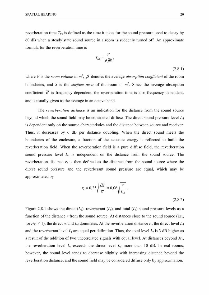
Figure 2.8.1 shows the direct (Ld), reverberant (Lr), and total (Lt) sound pressure levels as a
function of the distance r from the sound source. At distances close to the sound source (i.e.,
for r/rr < 1), the direct sound Ld dominates. At the reverberation distance rr, the direct level Ld
and the reverberant level Lr are equal per definition. Thus, the total level Lt is 3 dB higher as
a result of the addition of two uncorrelated signals with equal level. At distances beyond 3rr,
the reverberation level Lr exceeds the direct level Ld more than 10 dB. In real rooms,
however, the sound level tends to decrease slightly with increasing distance beyond the
reverberation distance, and the sound field may be considered diffuse only by approximation.
SPATIAL HEARING 21
Figure 2.8.1
Direct, reverberant, and total sound pressure levels in an enclosure as functions of thedistance from the sound source.
As mentioned in Section 2.5, the loudness cue for distance estimation is valid only in
anechoic environments since it is based on the decrease in sound pressure with increasing
distance from the source. Beyond the reverberation distance, which may be less than one
meter in average rooms, the total sound pressure level is almost constant, and the loudness
cue disappears. As the loudness cue becomes less effective with increasing reverberation, the
ratio D/R becomes more effective in distance perception. This ratio can be shown to be
( )( )
DR
PP
rr
rms
rms
r= =D
R
,
(2.8.3)
which is dependent only on the reverberation distance rr, a characteristic of the diffuse field
in the enclosure, and the distance r from the sound source. Therefore, D/R is considered to be
a much more effective distance cue than the loudness in a reverberant environment.
Furthermore, reverberation is considered to be important for the perception of the
environmental context. The reverberation time and level together with the experience with
sounds in reverberant rooms enable a listener to estimate the size and absorptiveness of the
surfaces in the environment.
Although, reverberation is important for distance and environmental context
perception, it was found to degrade the localisation accuracy of azimuth and elevation
[Begault, 1992 and 1994]. This is explained by the ability of humans to detect the direction of
the early reflections in severe reverberation conditions. The precedence effect mentioned in
Section 2.7 only partially suppresses the effects of reflected sounds. Moreover, the
0,1 1 10-20
-10
0
10
20
r/rr
Soun
d Pr
essu
re L
evel
[dB]
LrLdLt
SPATIAL HEARING 22
reverberation makes it difficult for the auditory system to correctly estimate the ITD at low
frequencies. This is because in typical rooms, the first reflections arrive before one period of
a low frequency cycle is completed. Thus, in a reverberant room, low frequency information
is essentially useless for localisation and azimuth localisation is severely degraded. In such
cases, the important timing information comes from the Interaural Envelope Difference
(IED), e.g. from the transients at the onset of a new sound.
2.9 Head-Related Transfer Functions
The most significant locationally dependent effect on the spectrum of a sound source can be
traced to the outer ears (pinnae), as mentioned in Section 2.4. This spectral filtering of a
sound source before it reaches the eardrum is usually termed the Head-Related Transfer
Function (HRTF). Within the literature, other terms equivalent to the term HRTF are used,
such as Head Transfer Function (HTF), Pinnae Transform, Outer Ear Transfer Function
(OETF), or Directional Transfer Function (DTF) [Møller, 1992].
From a psychoacoustic standpoint, the main role of HRTFs is thought to be the
disambiguation of front from back for sources on the cone of confusion, and, as an elevation
cue, the distinction of up from down. In fact, it can be shown that HRTFs capture all physical
cues to human sound localisation at once. This will be shown in the following by a discussion
of the basic physical properties of HRTFs.
HRTFs are functions in four variables, that is to say angle of incidence (ϕ and δ),
distance to the sound source (r), and frequency. If r is reasonably large (about one meter in
an anechoic environment), the source is said to be in the far field, and the response falls
inversely with the range as mentioned in Section 2.8. Most HRTF measurements are anechoic
far field measurements, which reduces an HRTF to be a function of three variables, namely
azimuth ϕ, elevation δ, and frequency.
HRTFs measured in an anechoic chamber do not include the effect of reverberation,
which is important for range estimation and environmental context perception. In that case,
unless binaural room simulation is used to introduce these important reflections, an improper
SPATIAL HEARING 23
ratio D/R results. When reproduced through headphones for example, the sound often seems
being either too close or inside the head1. It is possible, however, to measure the HRTFs in an
actual reverberant setting, but this has the disadvantage of limiting the simulated virtual
environment to a particular room and also leads to very long impulse responses.
Anechoic HRTFs of manikins and human subjects have been intensively studied in
search for physical characteristics that are related to sound localisation. For the present work,
a set of anechoic HRTFs measured on an acoustic manikin known as KEMAR by Gardner
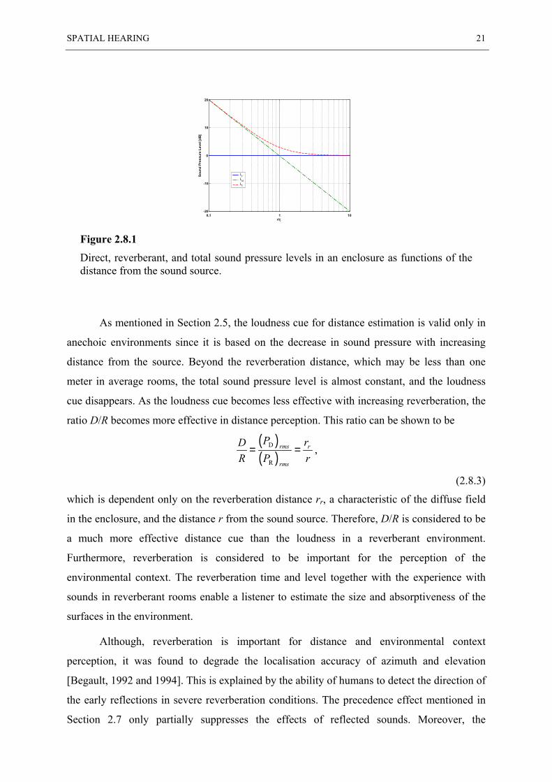
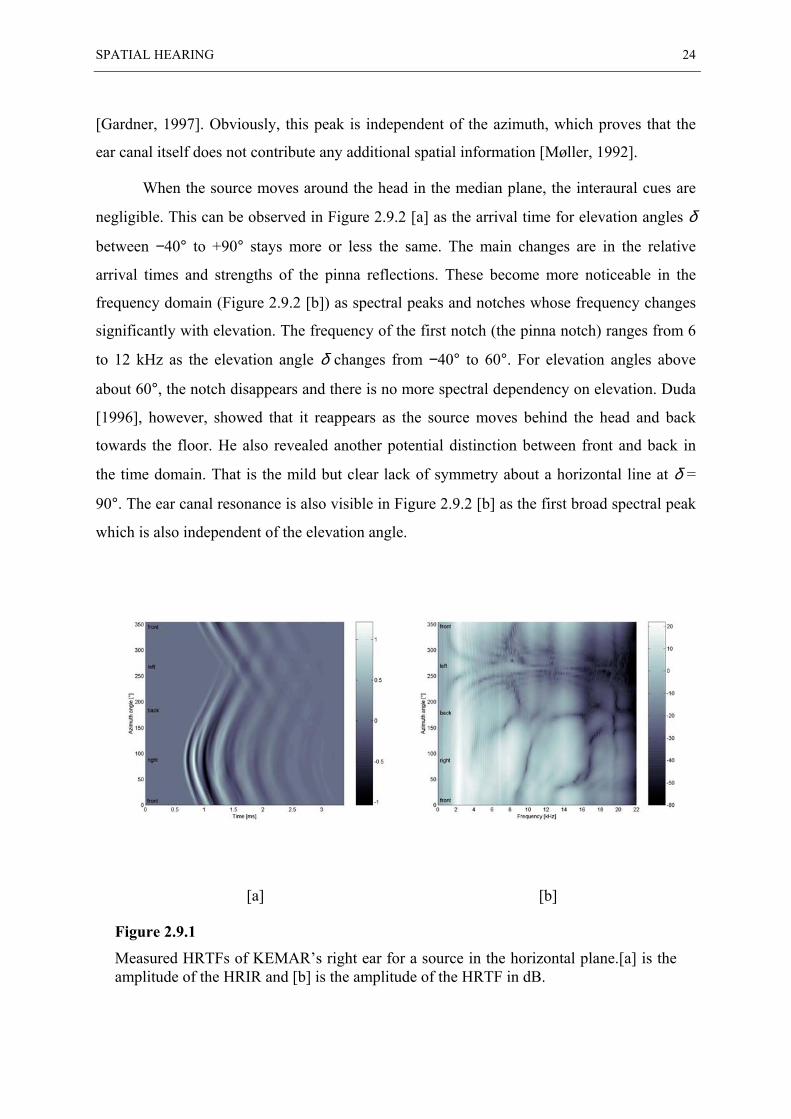
and Martin [1994], was used for the synthesis of virtual sound sources. Figure 2.9.1 [a] shows
the impulse response (the HRIR) of KEMAR’s right ear in the horizontal plane as a function
of the azimuth angle. The interaural cues can be readily recognised in this graph as the sound
has the highest amplitude and arrives first when it is coming from the right side (ϕ = 90°).
Conversely, it has the lowest amplitude and arrives latest when it is coming from the left side
(ϕ = 270°). The arrival time varies with azimuth in a more or less sinusoidal fashion as
estimated by a spherical head model [Blauert, 1997; Duda, 1996]. In fact, the arrival time
conforms quite well to the ITD equation (2.3.1). In particular, the difference between the
shortest and the longest arrival times is about 0.7 ms, just as the theory in Section 2.3
predicts.
Pinna reflections can also be noticed in the initial sequence of rapid changes when the
source is located at the right side of the head. The peak that arrives about 0.4 ms after the
initial peak is due to reflections off the shoulder. Finally, the cone of confusion phenomenon
can also be recognised as the response is almost symmetrical about the horizontal lines at
azimuth ϕ = 90° and ϕ = 270°, which constitute the interaural axis.
Figure 2.9.1 [b] shows the Fourier transform of the impulse response, i.e., the HRTF.
Also from this graph it can be clearly seen that the response is highest when the source is at
the right and weakest when the source is at the left. In addition, the pinna notch is easily
visible around 10 kHz when the source is at the right side of the head. For the opposite side,
the sound pressure is low due to head shadowing, and the notch appears not very clear. The
broad peak in the range between 2 and 3 kHz can be attributed to the ear canal resonance
1 This problem, which is very common particularly in headphone sound reproduction, is usually referred to as
Inside-Head Localisation (IHL).
SPATIAL HEARING 24
[Gardner, 1997]. Obviously, this peak is independent of the azimuth, which proves that the
ear canal itself does not contribute any additional spatial information [Møller, 1992].
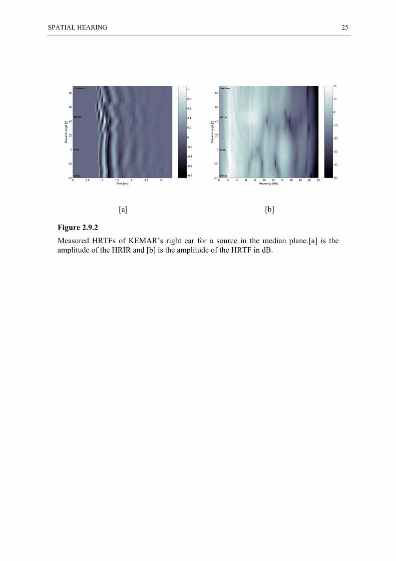
When the source moves around the head in the median plane, the interaural cues are
negligible. This can be observed in Figure 2.9.2 [a] as the arrival time for elevation angles δ
between −40° to +90° stays more or less the same. The main changes are in the relative
arrival times and strengths of the pinna reflections. These become more noticeable in the
frequency domain (Figure 2.9.2 [b]) as spectral peaks and notches whose frequency changes
significantly with elevation. The frequency of the first notch (the pinna notch) ranges from 6
to 12 kHz as the elevation angle δ changes from −40° to 60°. For elevation angles above
about 60°, the notch disappears and there is no more spectral dependency on elevation. Duda
[1996], however, showed that it reappears as the source moves behind the head and back
towards the floor. He also revealed another potential distinction between front and back in
the time domain. That is the mild but clear lack of symmetry about a horizontal line at δ =
90°. The ear canal resonance is also visible in Figure 2.9.2 [b] as the first broad spectral peak
which is also independent of the elevation angle.
[a] [b]
Figure 2.9.1
Measured HRTFs of KEMAR’s right ear for a source in the horizontal plane.[a] is theamplitude of the HRIR and [b] is the amplitude of the HRTF in dB.
SPATIAL HEARING 25
[a] [b]
Figure 2.9.2
Measured HRTFs of KEMAR’s right ear for a source in the median plane.[a] is theamplitude of the HRIR and [b] is the amplitude of the HRTF in dB.
Chapter 3 3D Sound Reproduction
3.1 Introduction
Psychoacousticians distinguish between the location of a sound source and the location of an
auditory event. The former is the position of a physical sound source in the listening space,
while the latter is the position where the listener experiences the sound [Blauert, 1997]. From
everyday experience, it is known that a monophonic audio signal played through a
loudspeaker makes the sound source and the auditory event locations coincide. However, it is
possible to process the audio signal so that the auditory event occurs at a different position in
the listening space than the position of the physical loudspeaker which actually emits the
sound. The listener perceives the sound to be coming from the auditory event position, which
is therefore referred to as a phantom or virtual sound source.
A simple form of this audio processing is the stereophonic audio system [AES, 1986],
where the amplitude or the phase of the sound is panned between two loudspeakers.
Stereophonic systems are able to position the virtual sound image at any point on the line
connecting the two loudspeakers. A direct extension to this technique is the surround sound
technique, where more than two loudspeakers surrounding the listener are used. By panning
the sound between every two adjacent loudspeakers, the auditory event can be positioned on
lines connecting the loudspeakers [Pulkki, 1997].
As the number of reproduction loudspeakers increases, the auditory event can be
accurately placed at any point in a three-dimensional (3D) space. This is exploited in the
wave field synthesis or holographic audio technique [Berkhout et al., 1993; Boone et al.,
3D SOUND REPRODUCTION 27
1995], which is based on the Kirchhoff-Helmholtz integral [Pierce, 1981]. The theory of the
Kirchhoff-Helmholtz integral suggests that any sound field can be reconstructed perfectly in
a given region by using a continuous layer of monopole and dipole sources. Although this is
currently impossible in practice, it represents the theoretical limiting case of exact sound field
reproduction.
In the present work, a more modest objective is considered, that is to say the problem
of reproducing a sound field locally at the eardrums of a listener. This approach requires far
fewer transducers than a system that attempts to reconstruct a complex sound field over a
relatively large area. As indicated in Chapter 1, the idea is to deliver binaural signals to the
ears of a listener. This is achieved by audio systems based on Head-Related Transfer
Functions (HRTFs). HRTF-based systems are also able to create multiple virtual sound
images simultaneously at different positions in the same listening space using two
loudspeakers only. This chapter introduces the basic principles behind virtual sound imaging
systems of this type.
3.2 Binaural Synthesis of Virtual Sound Sources
As discussed in Chapter 2, an HRTF measured from the source to the listener’s eardrum
captures all the physical cues to source localisation. This is also true if the HRTF was
measured at any point in the ear canals-possibly even a few millimetres outside and even
with a blocked ear canal, since all those measurements include the full spatial information
given to the ear [Møller, 1992]. Once the HRTFs corresponding to any desired position are
known, one can synthesise accurate binaural signals from any monaural source, and thus
place this source virtually at this desired location.
Consider the natural listening situation where a monophonic sound signal u(t)1 is
emitted from a source located at an arbitrary point (r, ϕ, δ) relatively to the centre of the
1 Note that this signal does not contain any spatial information.
3D SOUND REPRODUCTION 28
listener’s head. In principle, the sound pressure occurring in this situation at the listener’s
ears can be modelled by the convolution (filtering) between u(t) and the pair of Head-Related
Impulse Responses (HRIRs)1 between sound source and the listener’s left and right eardrums.
Conversely, filtering of the signal u(t) through the HRIR pair measured for a sound source at
the point (r, ϕ, δ) results in a pair of binaural signals which eventually create an auditory
event right at that measured point. This process-usually referred to as binaural synthesis-can
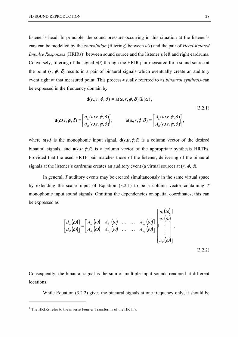
be expressed in the frequency domain by
)(),,,(),,,( ωδϕωδϕω urr ⋅= ad ,
(3.2.1)
,),,,(),,,(
),,,(
=
δϕωδϕω
δϕωrdrd
rR
Ld
=
),,,(),,,(
),,,(δϕωδϕω
δϕωrArA
rR
La ,
where u(ω) is the monophonic input signal, d(ω,r,ϕ,δ) is a column vector of the desired
binaural signals, and a(ω,r,ϕ,δ) is a column vector of the appropriate synthesis HRTFs.
Provided that the used HRTF pair matches those of the listener, delivering of the binaural
signals at the listener’s eardrums creates an auditory event (a virtual source) at (r, ϕ, δ).
In general, T auditory events may be created simultaneously in the same virtual space
by extending the scalar input of Equation (3.2.1) to be a column vector containing T
monophonic input sound signals. Omitting the dependencies on spatial coordinates, this can
be expressed as
( )( )
( ) ( ) ( )( ) ( ) ( )
( )( )
( )
⋅
=
ω
ωω
ωωωωωω
ωω
T
RRR
LLL
R
L
u
uu
AAAAAA
dd
T
T
M
MKK
KK 2
1
21
21 ,
(3.2.2)
Consequently, the binaural signal is the sum of multiple input sounds rendered at different
locations.
While Equation (3.2.2) gives the binaural signals at one frequency only, it should be
1 The HRIRs refer to the inverse Fourier Transforms of the HRTFs.
3D SOUND REPRODUCTION 29
kept in mind that there are as many equations of this form as there are frequencies. Assuming
the system is operating at a single frequency only, complex notation can be used to describe
the signals. Thus, it is assumed that all the signals are complex scalars. This allows the use of
well known matrix algebra for the proceeding discussion. Making those assumptions in the
following, the explicit dependency on the frequency ω may also be dropped to enhance the
readability of the equations. Thus, Equation (3.2.2) can be expressed in compact matrix
notation as
uAd ⋅= .
(3.2.3)
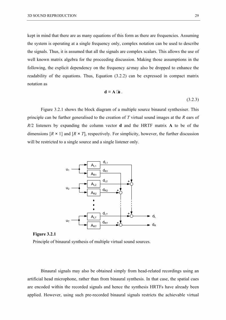
Figure 3.2.1 shows the block diagram of a multiple source binaural synthesiser. This
principle can be further generalised to the creation of T virtual sound images at the R ears of
R/2 listeners by expanding the column vector d and the HRTF matrix A to be of the
dimensions [R × 1] and [R × T], respectively. For simplicity, however, the further discussion
will be restricted to a single source and a single listener only.
Figure 3.2.1
Principle of binaural synthesis of multiple virtual sound sources.
Binaural signals may also be obtained simply from head-related recordings using an
artificial head microphone, rather than from binaural synthesis. In that case, the spatial cues
are encoded within the recorded signals and hence the synthesis HRTFs have already been
applied. However, using such pre-recorded binaural signals restricts the achievable virtual
dR
dL
dRT
dLT
dR2
dL2
dR1
dL1
u1
AL1
AR1
u2
AL2
AR2
uT
ALT
ART
+
+
+
+
3D SOUND REPRODUCTION 30
images to those already included with the recording. Subsequent processing in order to
manipulate the individual synthesis HRTFs is only possible with prior performing a
complicated unmixing procedure.
3.3 Headphone Displays
In 3D sound systems, the question arises of how to deliver the electrical binaural signals to
the listener’s eardrums as acoustic waves. In any case, the transmission paths from the
transducers to the listener’s ears (the listener’s HRTFs) have to be compensated in order to
correctly deliver the binaural signals. Headphones deliver dL at the left ear only and dR at the
right ear only, respectively, without any crosstalk from the opposite signal. Thus, the use of
headphones certainly simplifies the problem of transmission path inversion between the
transducers and the listener’s ears.
However, headphones have their own drawbacks: they may not be comfortable to
wear for a long time period. They also attenuate external sounds and isolate the user from the
surrounding environment. Sounds heard over headphones often seem to be too close or inside
the listener’s head as previously mentioned in Section 2.9. Since the physical sources (the
headphones) are actually very close to the listener’s ears, compensation is needed to
eliminate the acoustic cues to their locations. This compensation is very sensitive to the
headphone position. Finally, headphones can have notches and peaks in their frequency
responses that resemble the pinna responses. If uncompensated headphones are used,
elevation effects can be severely compromised [Duda, 1996].
3.4 Theory of Crosstalk Cancellation
3D SOUND REPRODUCTION 31
By using loudspeakers for binaural sound reproduction1, one can circumvent most of the
problems one encounters with headphone displays. However, as opposed to headphone
reproduction, the use of loudspeakers introduces the major problem of crosstalk. Thus, the
transmission path equalisation is considerably more difficult to achieve, since it also has to
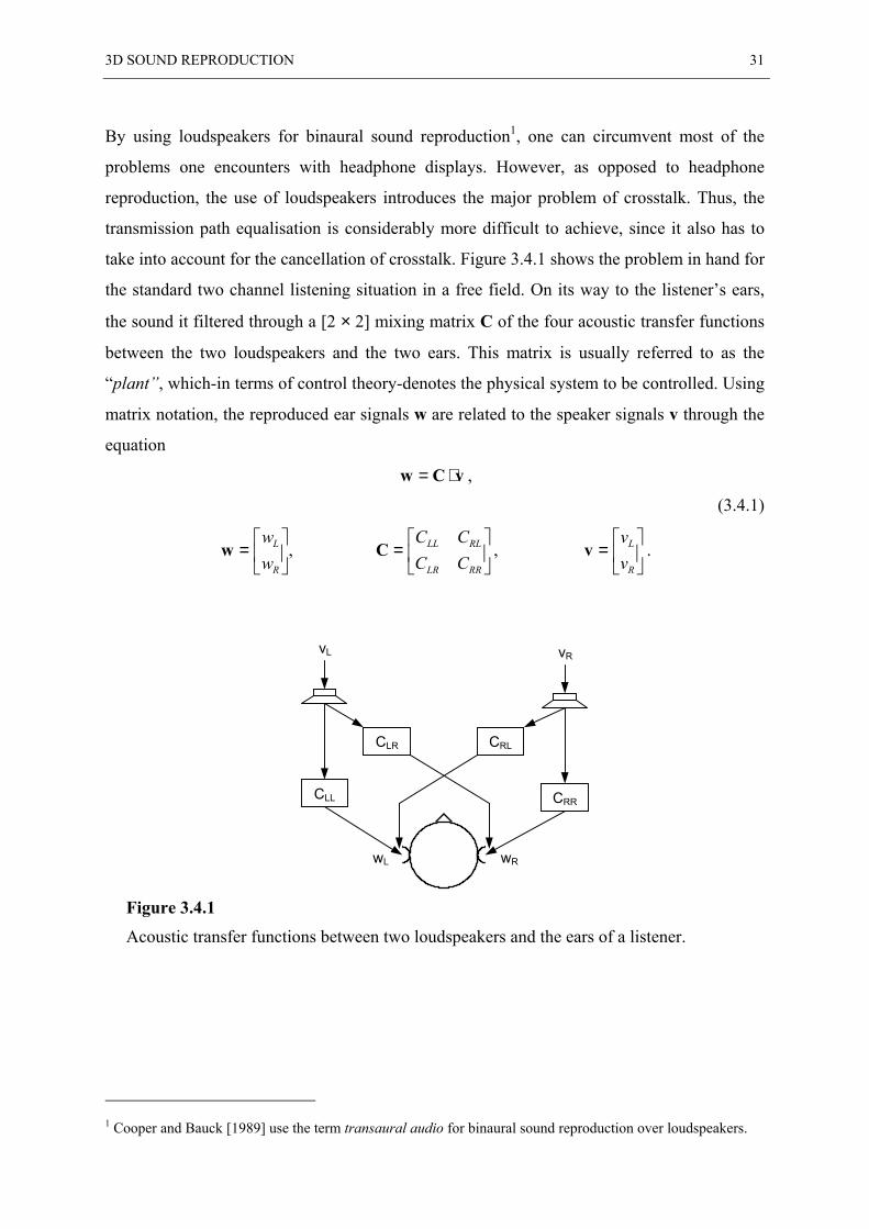
take into account for the cancellation of crosstalk. Figure 3.4.1 shows the problem in hand for
the standard two channel listening situation in a free field. On its way to the listener’s ears,
the sound it filtered through a [2 × 2] mixing matrix C of the four acoustic transfer functions
between the two loudspeakers and the two ears. This matrix is usually referred to as the
“plant”, which-in terms of control theory-denotes the physical system to be controlled. Using
matrix notation, the reproduced ear signals w are related to the speaker signals v through the
equation
vCw ⋅= ,
(3.4.1)
,
=
R
L
ww
w
=
RRLR
RLLL
CCCC
C ,
=
R
L
vv
v .
Figure 3.4.1
Acoustic transfer functions between two loudspeakers and the ears of a listener.
1 Cooper and Bauck [1989] use the term transaural audio for binaural sound reproduction over loudspeakers.
wRwL
vL vR
CRRCLL
CLR CRL
3D SOUND REPRODUCTION 32
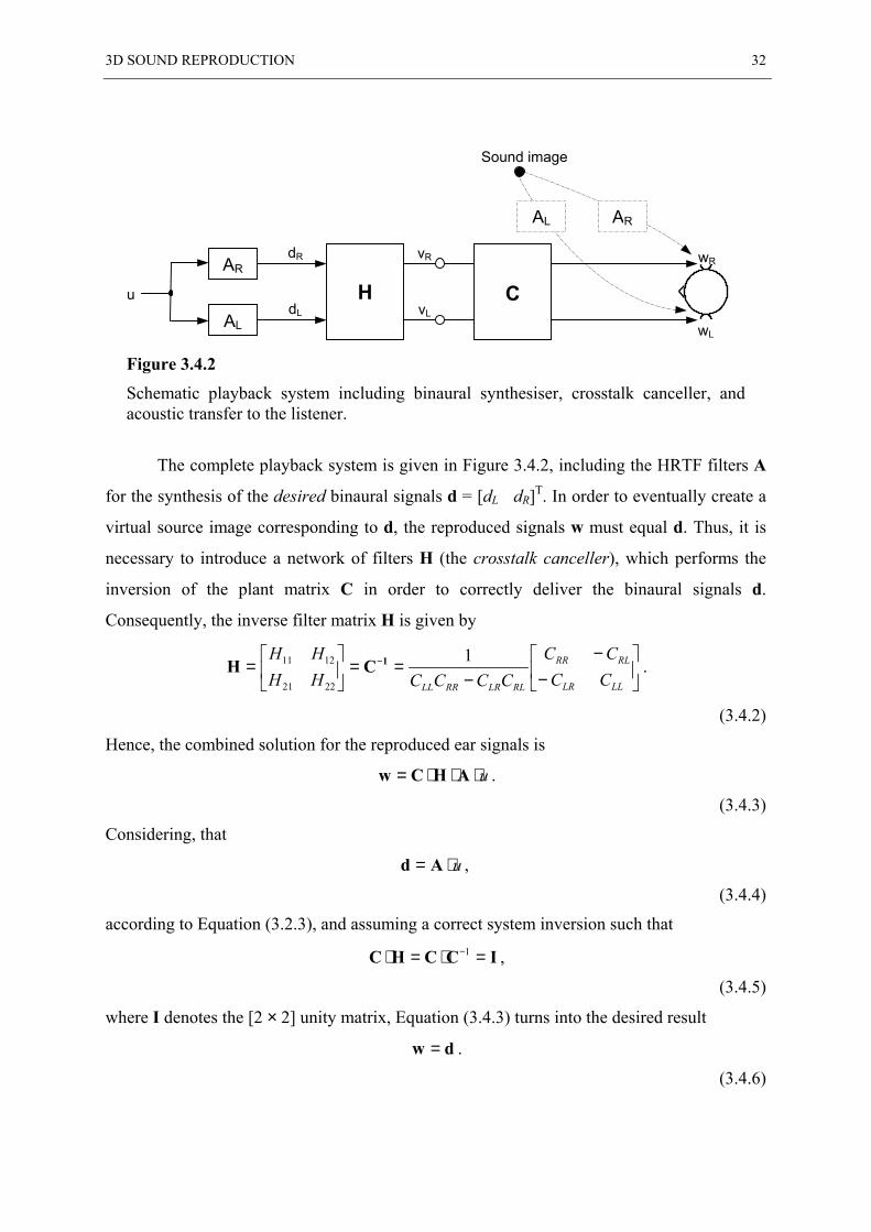
Figure 3.4.2
Schematic playback system including binaural synthesiser, crosstalk canceller, andacoustic transfer to the listener.
The complete playback system is given in Figure 3.4.2, including the HRTF filters A
for the synthesis of the desired binaural signals d = [dL dR]T. In order to eventually create a
virtual source image corresponding to d, the reproduced signals w must equal d. Thus, it is
necessary to introduce a network of filters H (the crosstalk canceller), which performs the
inversion of the plant matrix C in order to correctly deliver the binaural signals d.
Consequently, the inverse filter matrix H is given by
−
−−
==
= −
LLLR
RLRR
RLLRRRLL CCCC
CCCCHHHH 1
2221
1211 1CH .
(3.4.2)
Hence, the combined solution for the reproduced ear signals is
u⋅⋅⋅= AHCw .
(3.4.3)
Considering, that
u⋅= Ad ,
(3.4.4)
according to Equation (3.2.3), and assuming a correct system inversion such that
ICCHC =⋅=⋅ −1 ,
(3.4.5)
where I denotes the [2 × 2] unity matrix, Equation (3.4.3) turns into the desired result
dw = .
(3.4.6)
Sound image
vL
vR
dL
dR
CHAR
AL
u
AL AR
wL
wR
3D SOUND REPRODUCTION 33
In general, the ear signals w are considered to be measured by an ideal transducer
somewhere in the ear canal such that all direction-dependent features of the head response are
captured. Each of the functions CXY in the plant matrix C denote the transfer functions from
speaker X to ear Y and include the frequency response of loudspeaker and measurement
microphone as well as air propagation and the HRTF. Therefore, the elements of C are
complex functions in frequency and space coordinates. They are often said to be non-
minimum phase and contain deep notches due to the pinna reflections, particularly in
reverberant conditions. Moreover, since loudspeakers act like acoustic band-pass filters, their
responses lead to much less energy at the upper and lower ends of the audio frequency band.
For that reasons, the inversion of C required by the crosstalk cancellation matrix H in
Equation (3.4.2) is difficult to calculate. Considerations of achieving the system inversion by
means of numerical filtering will be discussed in Chapter 4.
3.5 Physical Interpretation of Crosstalk Cancellation
Usually, the plant transfer functions CXY are measured with a dummy head microphone.
Another measurement of the playback system only may be made with a single microphone
and no head present. The microphone (ideally the same as used for the dummy head
measurements) may be placed at the position where the centre of the dummy head was placed
before. Equalising the plant transfer functions with the inverse of this system response results
in a plant matrix
=
RRLR
RLLL
HHHH
C .
(3.5.1)
Thus, C now contains only the HRTFs normalised with respect to the free-field response at
the centre of the head, but with no head present. [Møller, 1992]. The inverse head transfer
matrix, regarding Equation (3.4.2) is now given as
3D SOUND REPRODUCTION 34
−
−== −
LLLR
RLRR
HHHH
D11CH RLLRRRLL HHHHD −= ,
(3.5.2)
where D is the determinant of the matrix C. The inverse determinant 1/D is common to all
terms and determines the stability of the inverse filter as will be shown in Chapter 4.
However, because it is a common factor, it only affects the overall equalisation and does not
affect crosstalk cancellation. When D is zero at any frequency, the matrix C is singular and
the inverse matrix H is undefined. Figure 3.5.1 shows the principle of a single source
binaural synthesiser cascaded with a crosstalk canceller. This block diagram is based on the
system suggested initially by Atal et al. [1966].
Dividing numerator and denominator by HLLHRR, Equation (3.5.2) can be rewritten as
RLL
R
RR
LL
ITFITFITFITF
HH
⋅−⋅
−
−⋅
=
11
11
1001
H ,
(3.5.3)
LL
LRL H
HITF =: ,RR
RLR H
HITF =:
Here, the ITF functions denote the so-called Interaural Transfer Functions, which describe
the difference in transmission to the ipsilateral and to the contralateral ear, respectively
[Møller, 1992].
Figure 3.5.1
Single source binaural synthesiser cascaded with a crosstalk canceller in block diagramform.
u
+−
−dR
dL vL
vR
1/DHRR
HLL 1/D
HRL
HLR
AL
AR+
3D SOUND REPRODUCTION 35
Observing Equation (3.5.3) reveals much about the physical process of crosstalk
cancellation. That is to say, crosstalk cancellation is effected by the ITF-terms in the off-
diagonal positions of the righthand matrix. These terms predict the crosstalk and send out an
out-of-phase cancellation signal into the opposite channel. For instance, the right input signal
is convolved with ITFR, which predicts the crosstalk that will reach the left ear, and the result
is subtracted from the left output signal. The common term 1/(1-ITFL·ITFR) compensates for
higher-order crosstalks, in other words, the fact that each crosstalk cancellation signal itself
transits to the opposite ear and must be cancelled by another cancellation signal. This
intrinsically recursive process, as recognised by Atal et al. [1966] will be further discussed in
the following section.
3.6 Stereo Dipole
As discussed above, the recursive nature of the crosstalk cancellation process gives rise to an
audible and hence undesirable frequency f0, usually referred to as the “ringing frequency”.
Obviously, this ringing frequency is also related to the time delay between the two
loudspeakers due to the finite distance between them. Thus, the value of f0 increases for
decreasing subtended angles 2θ 1. For a traditional stereo set-up with typically 2θ =60°, the
value of f0 is about 1,9 kHz, whereas with 2θ =10° the ringing frequency f0 becomes 10,8
kHz [Kirkeby et al., 1997]. Furthermore, it can be shown that the limiting case is equivalent
to a superposition of a point monopole and a point dipole source, both being placed at the
same point. A crosstalk cancellation system based on this source combination is considered
to be optimal since the reproduced sound field does not contain any “ringing” [Nelson et al.,
1997]. A system, referred to as the “Stereo Dipole” system, with a source span of 2θ =10° is
a good approximation of this theoretical set-up.
A free field simulation of the crosstalk cancellation principle is illustrated in Figure
1 The subtended angles, referred to as the loudspeaker span, are denoted here by 2θ (according to Figure 5.2.1).
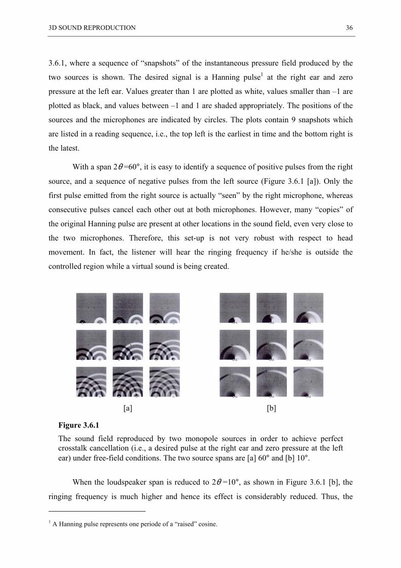
3D SOUND REPRODUCTION 36
3.6.1, where a sequence of “snapshots” of the instantaneous pressure field produced by the
two sources is shown. The desired signal is a Hanning pulse1 at the right ear and zero
pressure at the left ear. Values greater than 1 are plotted as white, values smaller than –1 are
plotted as black, and values between –1 and 1 are shaded appropriately. The positions of the
sources and the microphones are indicated by circles. The plots contain 9 snapshots which
are listed in a reading sequence, i.e., the top left is the earliest in time and the bottom right is
the latest.
With a span 2θ =60°, it is easy to identify a sequence of positive pulses from the right
source, and a sequence of negative pulses from the left source (Figure 3.6.1 [a]). Only the
first pulse emitted from the right source is actually “seen” by the right microphone, whereas
consecutive pulses cancel each other out at both microphones. However, many “copies” of
the original Hanning pulse are present at other locations in the sound field, even very close to
the two microphones. Therefore, this set-up is not very robust with respect to head
movement. In fact, the listener will hear the ringing frequency if he/she is outside the
controlled region while a virtual sound is being created.
Figu
Thecrosear)
ringing
1 A Han
[a] [b]
re 3.6.1
sound field reproduced by two monopole sources in order to achieve perfectstalk cancellation (i.e., a desired pulse at the right ear and zero pressure at the left under free-field conditions. The two source spans are [a] 60° and [b] 10°.
When the loudspeaker span is reduced to 2θ =10°, as shown in Figure 3.6.1 [b], the
frequency is much higher and hence its effect is considerably reduced. Thus, the
ning pulse represents one periode of a “raised” cosine.
3D SOUND REPRODUCTION 37
reproduced sound field is much simpler, and consequently, the area over which the sound
field can be controlled is larger. This suggests which was verified later by Takeuchi et al.
[1997], viz. that reducing the loudspeaker span 2θ improves the system’s robustness with
respect to head misalignment. In addition, since the ringing frequency and its harmonics are
more efficiently suppressed, the reproduced sound results in a more natural quality.
However, as the ringing frequency is increased, it is obvious that the adjacent pulses
overlap increasingly. Thus, it is also intuitively obvious that by increasing f0, the low-
frequency content of the signals is also increased. Consequently, in order to achieve perfect
crosstalk cancellation with a pair of closely spaced loudspeakers, a very large low-frequency
output is necessary. This happens because the crosstalk cancellation problem is said to be ill-
conditioned at low frequencies (see Section 4.7). In the case of virtual source imaging, i.e.,
when one attempts to produce a sound at both ears rather than at one ear only, the low-
frequency content is reduced because the positive and negative parts of the pulse trains cancel
each other out. Therefore, it is an easier task to create a virtual sound image than to achieve
perfect crosstalk cancellation [Kirkeby et al., 1997]. However, creating virtual sources well
outside 2θ still requires a considerable amount of low frequency, especially with a small
loudspeaker span.
Fortunately, though, as long as the loudspeaker span is not too small only a moderate
boost of low frequencies is required. In practice, the “Stereo Dipole” system with a
loudspeaker span of 10° is a good compromise.
Chapter 4 Inverse Filter Design
4.1 Introduction
The control filters in loudspeaker displays must implement both binaural synthesis and
crosstalk cancellation functions as discussed in the previous chapter. The task of the crosstalk
cancellation subsystem is to invert a matrix C of electro-acoustic transfer functions.
In practice, the exact inverse is difficult to calculate and in some cases, may not be
possible to achieve at certain frequencies. Only when C is a minimum phase system, it is
possible to achieve a stable time response for the inverse filter H. Basically, a minimum
phase signal has a minimum delay property, which effectively guarantees that the signal has
its energy concentrated at its start [Oppenheim and Schafer, 1975]. However, the electro-
acoustic transfer functions contained in C are not likely to be minimum phase, since they
contain echoes due to pinna reflections and the room response. If the impulse response of the
inverse of such a signal has to be stable, it generally has to start before time zero, hence, it is
said to be non-causal. In fact, the exact inverse of a non-minimum phase system has an
impulse response which begins infinitely far back in time. Another problem encountered with
the system inversion is that if C(ω) is very small within a narrow range of frequencies, the
inversion H(ω) = 1/C(ω) becomes very large. Such problems are said to be ill-conditioned.
Finally, since the performance of a digital filter is inevitably limited by the number of filter
coefficients, it is not realistic to expect an exact inversion.
However, by aiming at an approximation rather than at the exact inversion, it is
possible to design a digital finite impulse response (FIR) filter, such that the system is
INVERSE FILTER DESIGN 39
inverted (deconvolved) almost perfectly. Obviously, a good approximation is characterised by
being close, in some sense, to the exact solution. In order to be able to find the best
approximation, it is necessary to have a measure for the difference between the two: a ”cost
function”1. The most common choice is to use a cost function which is a time average of the
squared deviations (the error) between the desired output and the actual output from the
system.
Various methods for multi-channel inverse filter design have been suggested, both in
the time and frequency domain. Most of them apply the principle of minimisation or
optimisation in this “statistical” least squares sense. Initially, the principle of multi-channel
inverse filtering has been widely used in active noise control systems [Nelson and Elliott,
1992]. In terms of signal processing, the suppression of an unwanted sound and the
reproduction of a desired sound turn out to be very similar problems. Therefore, it is fairly
straightforward to apply these inverse filtering techniques also to sound reproduction
systems.
A very versatile adaptive time domain algorithm is the steepest descent Least-Mean-
Square (LMS) algorithm [Widrow and Stearns, 1985]. The method of fast deconvolution
using regularisation, on the other hand, is based on determining the inverse (FIR) filters in
the frequency domain, and was applied on multi-channel systems by Kirkeby et al. [1996a].
This method as well as a general study of the mentioned problems in digital inverse filter
design will be discussed in the following sections of this chapter.
4.2 Exact Inversion of Single Channel Systems
For the study of inverse filter design, the first requirement is an understanding of the basic
problems in the simplest case: the single channel case. The acoustic path between a source
and a receiver can be thought as a filter of a particular length. Representing this filter as a
discrete-time system, it may be analysed by using the z-transform [Oppenheim and Schafer,
1975]
1 Sometimes also called “error function” or “performance index”
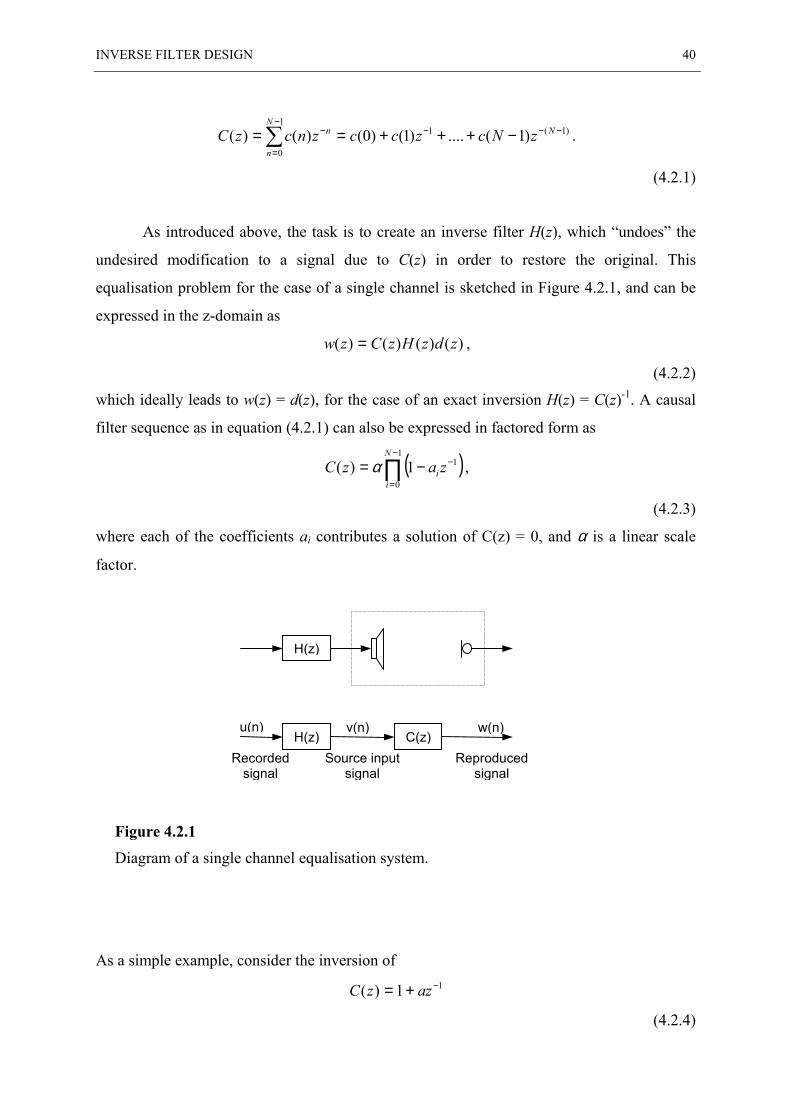
INVERSE FILTER DESIGN 40
)1(11
0)1(....)1()0()()( −−−
−
=
− −+++==∑ NN
n
n zNczccznczC .
(4.2.1)
As introduced above, the task is to create an inverse filter H(z), which “undoes” the
undesired modification to a signal due to C(z) in order to restore the original. This
equalisation problem for the case of a single channel is sketched in Figure 4.2.1, and can be
expressed in the z-domain as
)()()()( zdzHzCzw = ,
(4.2.2)
which ideally leads to w(z) = d(z), for the case of an exact inversion H(z) = C(z)-1. A causal
filter sequence as in equation (4.2.1) can also be expressed in factored form as
( )∏−
=
−−=1
0
11)(N
ii zazC α ,
(4.2.3)
where each of the coefficients ai contributes a solution of C(z) = 0, and α is a linear scale
factor.
Figure 4.2.1
Diagram of a single channel equalisation system.
As a simple example, consider the inversion of11)( −+= azzC
(4.2.4)
u(n)
H(z)
H(z) C(z)v(n) w(n)
Recordedsignal
Source inputsignal
Reproducedsignal

INVERSE FILTER DESIGN 41
to give an illustration of the problems involved in the single channel inversion. The inverse
filter may be first calculated directly as
111
)(1)( −+
==azzC
zH .
(4.2.5)
Observing equation (4.2.5) reveals that the zero of C(z) is now mapped into a pole of the
inverse filter function H(z). In general, an exact inversion of C(z) always maps the poles of
C(z) to the zeros of H(z), and the zeros of C(z) to the poles of H(z), respectively.
For the underlying example, two different cases have to be investigated in order to
determine the inverse filter in the z-domain and in terms of the corresponding pole-zero map.
• For the case that |a| < 1, using the binomial expansion
( ) ....1 )1(1 32
0
1 +−+−=−=+ ∑∞
=
− xxxxxk
kk ,
(4.2.6)
the inverse filter H can be turned into the all-zero model
( ) ....1 )(1)( 33221
0
11 +−+−=−=+= −−−∞
=
−−− ∑ zazaazzaazzHn
nn
(4.2.7)
This geometric series shows that, due to |a| < 1, the sequence is causal and convergent.
Thus, the designed inverse filter is causal and stable. The pole of H(z) is inside the unit circle
as can be observed in the pole-zero map of Figure 4.2.2. In general, a filter system with all its
zeros inside the unit circle, as C(z) is in this case, is called a minimum-phase system.
• For the case that |a| > 1, the filter system C in Equation (4.2.4) has its zero outside the
unit circle, and therefore, it is called a non-minimum phase system. Actually, systems
with all their zeros outside the unit circle are generally called maximum phase. On the
contrary, systems with some zeros inside the unit circle and the remaining zeros outside
the unit circle are usually referred to as non-minimum phase or mixed-phase systems
[Proakis and Manolakis, 1996]. For the present system, the inverse filter H can be turned
into an all-zero model by exploiting the geometric series as
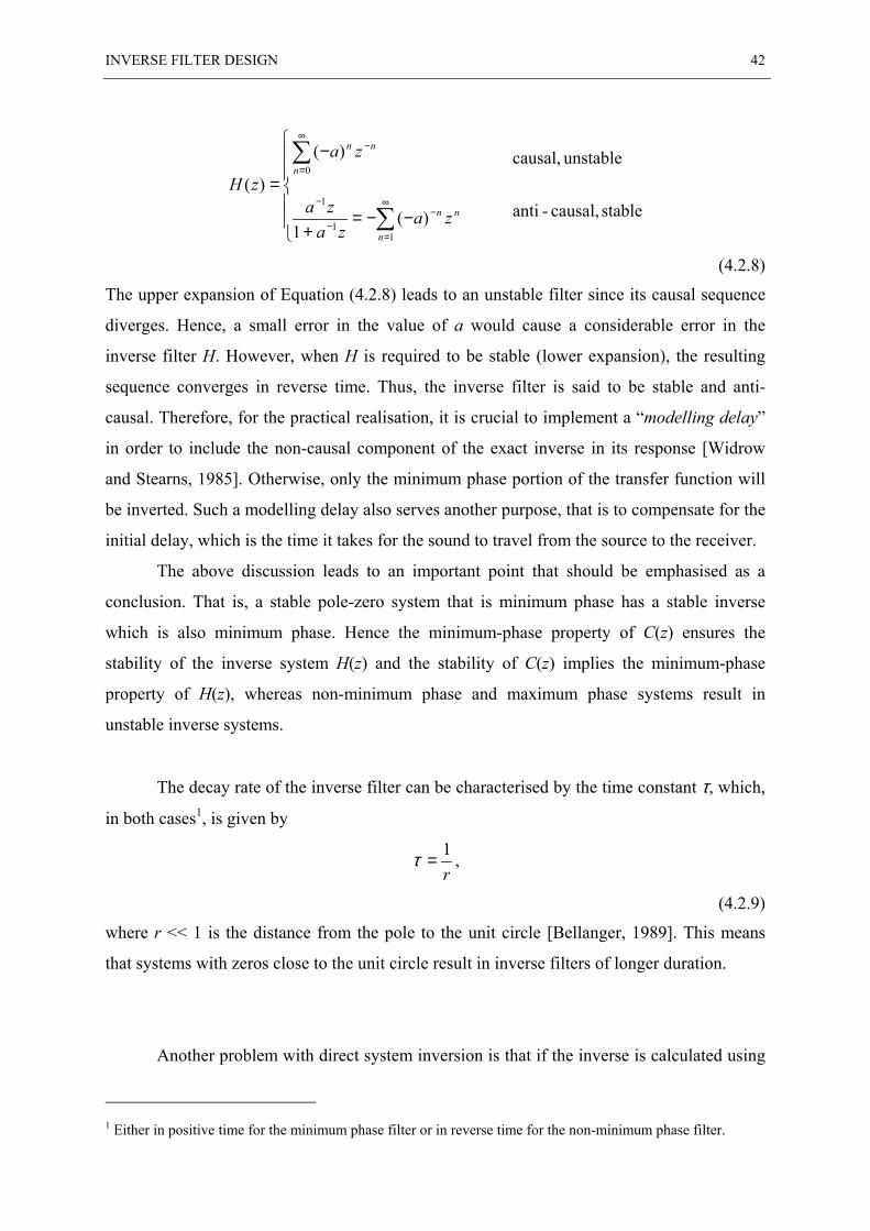
INVERSE FILTER DESIGN 42
stable causal,-anti
unstable causal,
)(1
)(
)(
11
1
0
−−=+
−
=
∑
∑
∞
=
−−
−
∞
=
−
n
nn
n
nn
zaza
za
za
zH
(4.2.8)
The upper expansion of Equation (4.2.8) leads to an unstable filter since its causal sequence
diverges. Hence, a small error in the value of a would cause a considerable error in the
inverse filter H. However, when H is required to be stable (lower expansion), the resulting
sequence converges in reverse time. Thus, the inverse filter is said to be stable and anti-
causal. Therefore, for the practical realisation, it is crucial to implement a “modelling delay”
in order to include the non-causal component of the exact inverse in its response [Widrow
and Stearns, 1985]. Otherwise, only the minimum phase portion of the transfer function will
be inverted. Such a modelling delay also serves another purpose, that is to compensate for the
initial delay, which is the time it takes for the sound to travel from the source to the receiver.
The above discussion leads to an important point that should be emphasised as a
conclusion. That is, a stable pole-zero system that is minimum phase has a stable inverse
which is also minimum phase. Hence the minimum-phase property of C(z) ensures the
stability of the inverse system H(z) and the stability of C(z) implies the minimum-phase
property of H(z), whereas non-minimum phase and maximum phase systems result in
unstable inverse systems.
The decay rate of the inverse filter can be characterised by the time constant τ, which,
in both cases1, is given by
r1=τ ,
(4.2.9)
where r << 1 is the distance from the pole to the unit circle [Bellanger, 1989]. This means
that systems with zeros close to the unit circle result in inverse filters of longer duration.
Another problem with direct system inversion is that if the inverse is calculated using
1 Either in positive time for the minimum phase filter or in reverse time for the non-minimum phase filter.
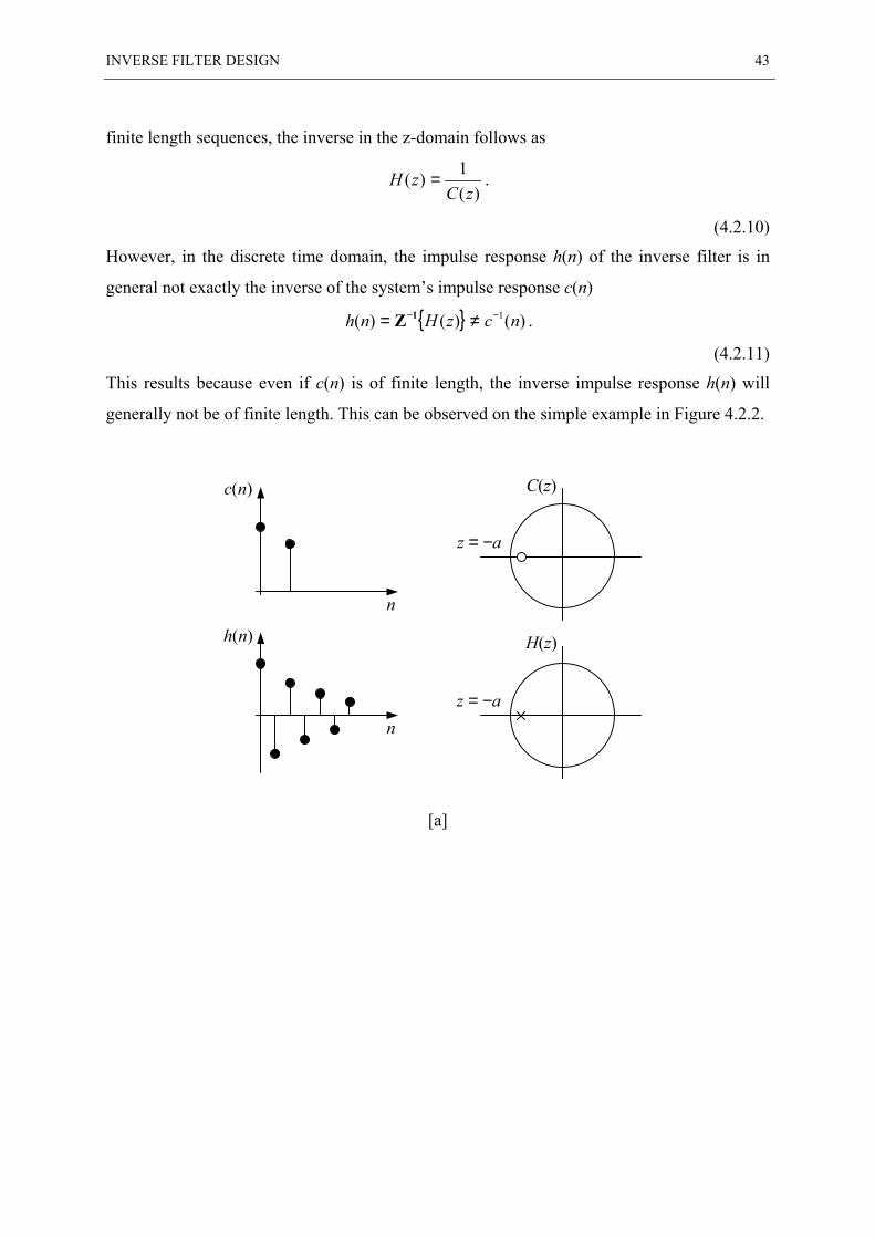
INVERSE FILTER DESIGN 43
finite length sequences, the inverse in the z-domain follows as
)(1)(zC
zH = .
(4.2.10)
However, in the discrete time domain, the impulse response h(n) of the inverse filter is in
general not exactly the inverse of the system’s impulse response c(n)
{ } )()()( 1 nczHnh −− ≠= 1Z .
(4.2.11)
This results because even if c(n) is of finite length, the inverse impulse response h(n) will
generally not be of finite length. This can be observed on the simple example in Figure 4.2.2.
[a]
c(n)
n
C(z)
z = −a
H(z)
z = −a
h(n)
n
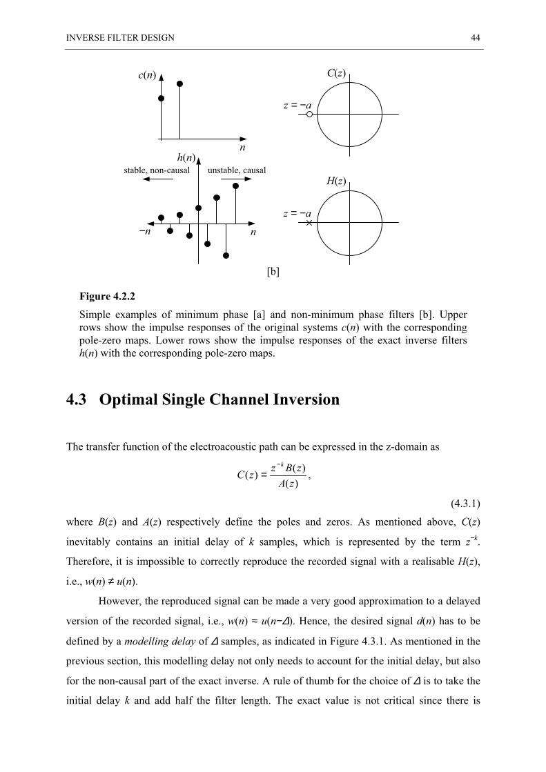
INVERSE FILTER DESIGN 44
[b]
Figure 4.2.2
Simple examples of minimum phase [a] and non-minimum phase filters [b]. Upperrows show the impulse responses of the original systems c(n) with the correspondingpole-zero maps. Lower rows show the impulse responses of the exact inverse filtersh(n) with the corresponding pole-zero maps.
4.3 Optimal Single Channel Inversion
The transfer function of the electroacoustic path can be expressed in the z-domain as
)()()(
zAzBzzC
k−
= ,
(4.3.1)
where B(z) and A(z) respectively define the poles and zeros. As mentioned above, C(z)
inevitably contains an initial delay of k samples, which is represented by the term z−k.
Therefore, it is impossible to correctly reproduce the recorded signal with a realisable H(z),
i.e., w(n) ≠ u(n).
However, the reproduced signal can be made a very good approximation to a delayed
version of the recorded signal, i.e., w(n) ≈ u(n−∆). Hence, the desired signal d(n) has to be
defined by a modelling delay of ∆ samples, as indicated in Figure 4.3.1. As mentioned in the
previous section, this modelling delay not only needs to account for the initial delay, but also
for the non-causal part of the exact inverse. A rule of thumb for the choice of ∆ is to take the
initial delay k and add half the filter length. The exact value is not critical since there is
c(n)
n
C(z)
z = −a
H(z)
z = −a
h(n)
n−n
stable, non-causal unstable, causal
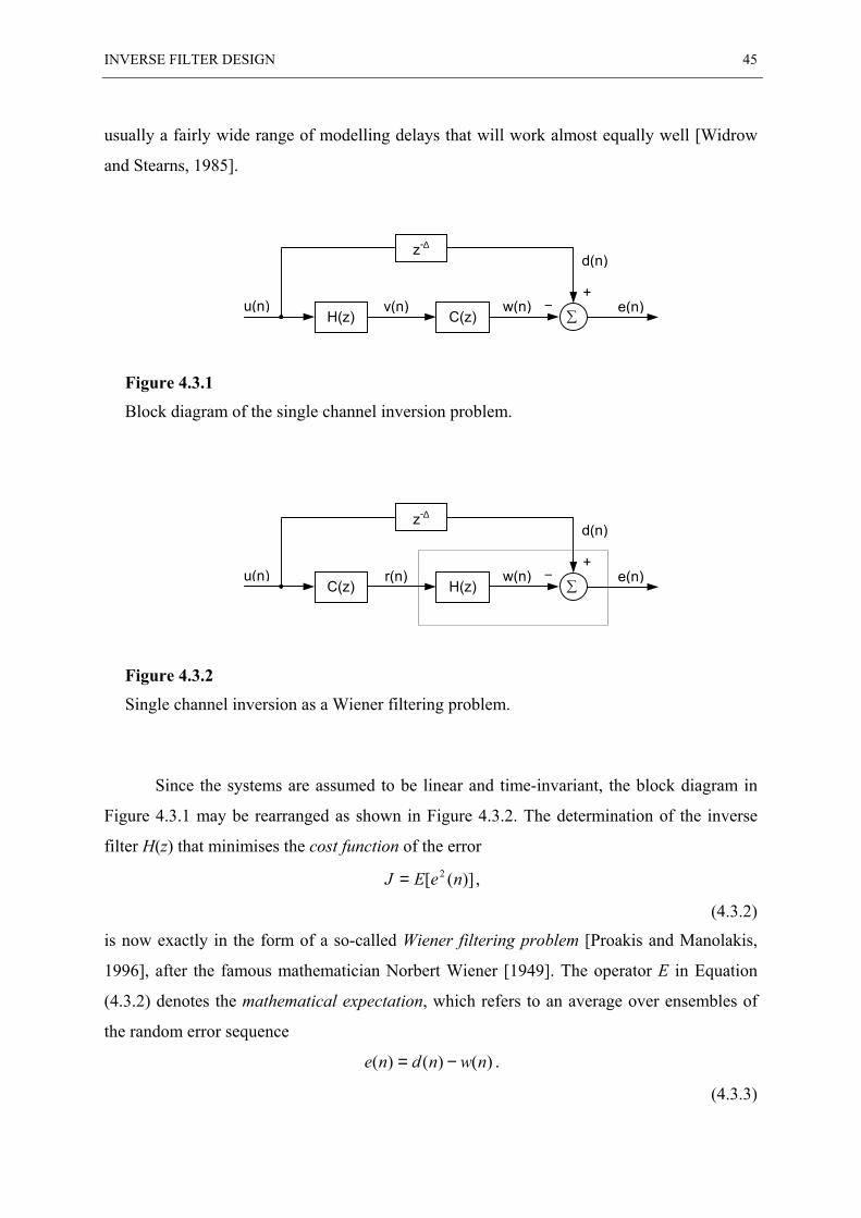
INVERSE FILTER DESIGN 45
usually a fairly wide range of modelling delays that will work almost equally well [Widrow
and Stearns, 1985].
Figure 4.3.1
Block diagram of the single channel inversion problem.
Figure 4.3.2
Single channel inversion as a Wiener filtering problem.
Since the systems are assumed to be linear and time-invariant, the block diagram in
Figure 4.3.1 may be rearranged as shown in Figure 4.3.2. The determination of the inverse
filter H(z) that minimises the cost function of the error
)]([ 2 neEJ = ,
(4.3.2)
is now exactly in the form of a so-called Wiener filtering problem [Proakis and Manolakis,
1996], after the famous mathematician Norbert Wiener [1949]. The operator E in Equation
(4.3.2) denotes the mathematical expectation, which refers to an average over ensembles of
the random error sequence
)()()( nwndne −= .
(4.3.3)
u(n)H(z)
v(n) w(n)
z-∆
C(z) ∑−
+
d(n)
e(n)
u(n)C(z)
r(n) w(n)
z-∆
H(z) ∑−
+
d(n)
e(n)
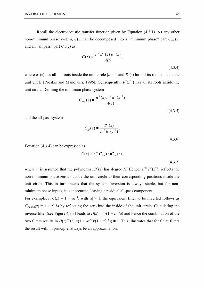
INVERSE FILTER DESIGN 46
Recall the electroacoustic transfer function given by Equation (4.3.1). As any other
non-minimum phase system, C(z) can be decomposed into a “minimum phase” part Cmin(z)
and an “all pass” part Cap(z) as
A(z)zBzBzzC
k )( )()(−+−
= ,
(4.3.4)
where B+(z) has all its roots inside the unit circle |z| = 1 and B−(z) has all its roots outside the
unit circle [Proakis and Manolakis, 1996]. Consequently, B−(z−1) has all its roots inside the
unit circle. Defining the minimum phase system
)()()()(
1
zAzBzzBzC
N
min
−−−+
=
(4.3.5)
and the all-pass system
)()()( 1−−−
−
=zBz
zBzC Nap ,
(4.3.6)
Equation (4.3.4) can be expressed as
)()()( zCzCzzC apmink−= ,
(4.3.7)
where it is assumed that the polynomial B−(z) has degree N. Hence, z−N B−(z−1) reflects the
non-minimum phase zeros outside the unit circle to their corresponding positions inside the
unit circle. This in turn means that the system inversion is always stable, but for non-
minimum phase inputs, it is inaccurate, leaving a residual all-pass component.
For example, if C(z) = 1 + az−1, with |a| > 1, the equivalent filter to be inverted follows as
Ceq,min(z) = 1 + z−1/a by reflecting the zero into the inside of the unit circle. Calculating the
inverse filter (see Figure 4.3.3) leads to H(z) = 1/(1 + z−1/a) and hence the combination of the
two filters results in H(z)⋅C(z) =(1 + az−1)/(1 + z−1/a) ≠ 1. This illustrates that for finite filters
the result will, in principle, always be an approximation.
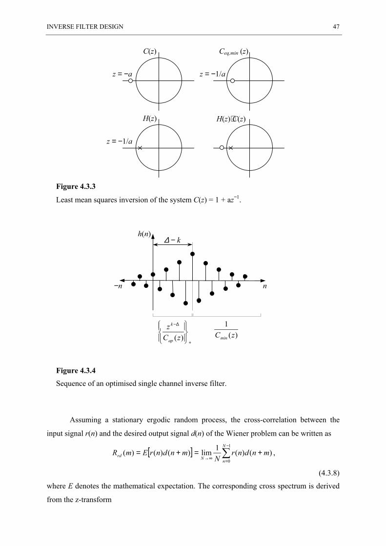
INVERSE FILTER DESIGN 47
Figure 4.3.3
Least mean squares inversion of the system C(z) = 1 + az−1.
Figure 4.3.4
Sequence of an optimised single channel inverse filter.
Assuming a stationary ergodic random process, the cross-correlation between the
input signal r(n) and the desired output signal d(n) of the Wiener problem can be written as
[ ] ∑−
=∞→+=+=
1
0)()(1lim)()()(
N
nNrd mndnrN
mndnrEmR ,
(4.3.8)
where E denotes the mathematical expectation. The corresponding cross spectrum is derived
from the z-transform
Ceq,min (z)
z = −1/a
H(z)⋅C(z)
C(z)
z = −a
H(z)
z = −1/a
h(n)
n−n
∆ − k
+
∆−
)(zCz
ap
k
)(1
zCmin
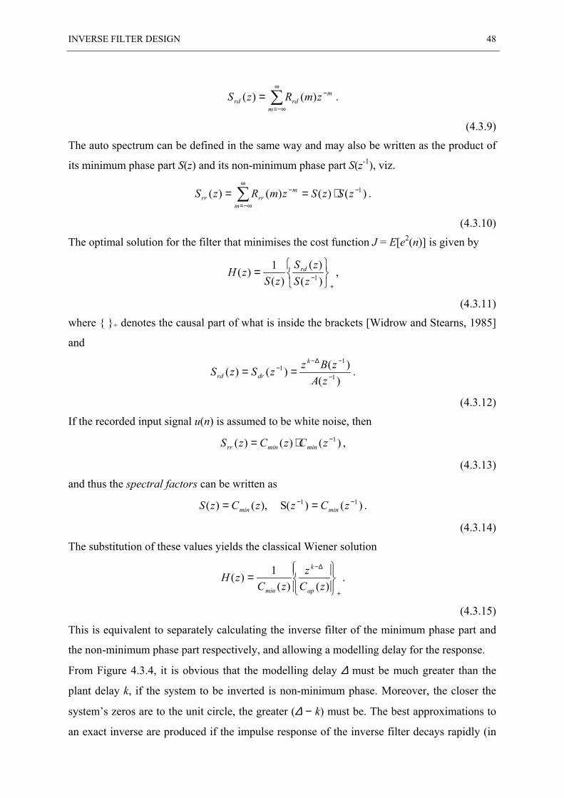
INVERSE FILTER DESIGN 48
∑∞
−∞=
−=m
mrdrd zmRzS )()( .
(4.3.9)
The auto spectrum can be defined in the same way and may also be written as the product of
its minimum phase part S(z) and its non-minimum phase part S(z-1), viz.
)()()()( 1−∞
−∞=
− ⋅== ∑ zSzSzmRzSm
mrrrr .
(4.3.10)
The optimal solution for the filter that minimises the cost function J = E[e2(n)] is given by
+−
=)()(
)(1)( 1zS
zSzS
zH rd ,
(4.3.11)
where { }+ denotes the causal part of what is inside the brackets [Widrow and Stearns, 1985]
and
)()()()( 1
11
−
−∆−− ==
zAzBzzSzS
k
drrd .
(4.3.12)
If the recorded input signal u(n) is assumed to be white noise, then
)()()( 1−⋅= zCzCzS minminrr ,
(4.3.13)
and thus the spectral factors can be written as
)()(S ),()( 11 −− == zCzzCzS minmin .
(4.3.14)
The substitution of these values yields the classical Wiener solution
+
∆−
=)()(
1)(zC
zzC
zHap
k
min
.
(4.3.15)
This is equivalent to separately calculating the inverse filter of the minimum phase part and
the non-minimum phase part respectively, and allowing a modelling delay for the response.
From Figure 4.3.4, it is obvious that the modelling delay ∆ must be much greater than the
plant delay k, if the system to be inverted is non-minimum phase. Moreover, the closer the
system’s zeros are to the unit circle, the greater (∆ − k) must be. The best approximations to
an exact inverse are produced if the impulse response of the inverse filter decays rapidly (in
INVERSE FILTER DESIGN 49
forward or reverse time) compared to the available filter length.
4.4 Regularisation
The technique of zero’th order regularisation [Press et al., 1992] is traditionally used when
one encounters ill-conditioned inversion problems, as will be discussed later in Section 4.7.
Basically, regularisation implies an optimisation process of the “effort” which is put into the
system by means of the source input signal v(n). This is done in addition to the optimisation
of the inverse filtering error “performance”. Correspondingly, the inverse filter H(z) has now
to be designed in order to minimise the modified cost function
)]([)]([ 22 nvEβneEJ += ,
(4.4.1)
The regularisation parameter β is a positive real constant that determines how much weight
to assign to the effort term E[v2(n)]. By varying β from zero to infinity, the solution changes
gradually from minimising the performance E[e2(n)] only to minimising the effort cost
E[v2(n)] only. Thus, regularisation represents a trade-off process between effort cost and
performance error in a way that a large value of β will minimise the effort at the expense of
the performance and vice versa for a small value of β.
The optimal solution for the Wiener filter which minimises J in that case is then given by
+
−
−∆−
=)()()(
)(1)( 1
1
zCzSzCz
zSzH
ap
mink
,
(4.4.2)
where, for white noise at the input u(n),
βzCzCβzSzSzS minminrr +=+= −− )()()()()( 11 .
(4.4.3)
Since a large value of β means that the optimal solution will favour a low power
output from the inverse filters (low effort) at the expense of a low performance, the physical
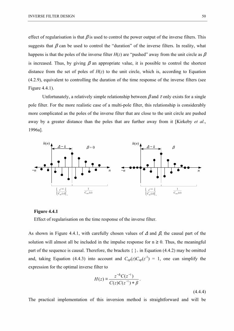
INVERSE FILTER DESIGN 50
effect of regularisation is that β is used to control the power output of the inverse filters. This
suggests that β can be used to control the “duration” of the inverse filters. In reality, what
happens is that the poles of the inverse filter H(z) are “pushed” away from the unit circle as β
is increased. Thus, by giving β an appropriate value, it is possible to control the shortest
distance from the set of poles of H(z) to the unit circle, which is, according to Equation
(4.2.9), equivalent to controlling the duration of the time response of the inverse filters (see
Figure 4.4.1).
Unfortunately, a relatively simple relationship between β and τ only exists for a single
pole filter. For the more realistic case of a multi-pole filter, this relationship is considerably
more complicated as the poles of the inverse filter that are close to the unit circle are pushed
away by a greater distance than the poles that are further away from it [Kirkeby et al.,
1996a].
Figure 4.4.1
Effect of regularisation on the time response of the inverse filter.
As shown in Figure 4.4.1, with carefully chosen values of ∆ and β, the causal part of the
solution will almost all be included in the impulse response for n ≥ 0. Thus, the meaningful
part of the sequence is causal. Therefore, the brackets { }+ in Equation (4.4.2) may be omitted
and, taking Equation (4.4.3) into account and Cap(z)Cap(z-1) = 1, one can simplify the
expression for the optimal inverse filter to
βzCzCzCzzH
+= −
−∆−
)()()()( 1
1
.
(4.4.4)
The practical implementation of this inversion method is straightforward and will be
h(n)
n−n
∆ − k
+
∆−
)(zCz
ap
k
)(1
zCmin
h(n)
n−n
∆ − k
+
∆−
)(zCz
ap
k
)(1
zCmin
β = 0 β
INVERSE FILTER DESIGN 51
explained later in Section 4.6.
4.5 Multi-Channel System Inversion
The generalised inversion problem for a multi-channel sound reproduction system is shown
in the block diagram in Figure 4.5.1. The variables are defined in the same way as in the
single channel case but now all the signals are represented by vectors and all the filters are
represented by matrices of a certain dimension. Define u(z) as a vector of T input signals, v(z)
as a vector of S source input or loudspeaker signals, w(z) as vector of R reproduced signals,
d(z) as a vector of R desired signals, and e(z) as a vector of R error signals. All vectors are
column vectors, so that
=
)(
)()(
1
zU
zUz
T
Mu ,
=
)(
)()(
1
zV
zVz
S
Mv ,
=
)(
)()(
1
zW
zWz
R
Mw ,
=
)(
)()(
1
zD
zDz
R
Md ,
=
)(
)()(
1
zE
zEz
R
Me .
(4.5.1)
Correspondingly, the multi-channel filters have the following structures: A(z) is an [R × T]
target matrix, C(z) is an [R × S] plant (electroacoustic) matrix, and H(z) is [S × T] matrix of
inverse filters.
=
)()(
)()()(
1
111
zAzA
zAzAz
RTR
T
L
MOM
L
A
=
)()(
)()()(
1
111
zCzC
zCzCz
RSR
S
L
MOM
L
C
(4.5.2)
=
)()(
)()()(
1
111
zHzH
zHzHz
STS
T
L
MOM
L
H
From the block diagram shown in Figure 4.5.1, it is straightforward to derive the following
relationships:
INVERSE FILTER DESIGN 52
)()()( zzz uHv = , a)
)()()( zzz uAd = , b)
)()()( zzz vCw = , c)
)()()( zzz wde −= . d)
(4.5.3)
For a multi-channel system, the aim is now to determine a matrix of inverse filters H(z) that
minimises the quadratic cost function
)]()([)]()([ nnEβnnEJ TT vvee += ,
(4.5.4)
where the superscript T denotes the transpose of its argument. As a generalisation of the
single channel case [Kirkeby et al., 1996a], the optimal solution for the inverse filter matrix
is given by
)()(])()([)( 1110 zzβzzz TT ACICCH −−− += .
(4.5.5)
In the present work, the system was restricted to a conventional two channel sound
reproduction system and one listener, i.e., the number of sources S = 2 and the number of
reproduced signals, or receivers, R = 2. For the purpose of crosstalk cancellation with such a
system, the inverse filters have to ensure that independent desired signals d(z) are reproduced
at the 2 ears of a listener. In this case, the target matrix A(z)=z-∆I, where I denotes a unity
matrix of order R = T (see Section 3.4). With no modelling delay (∆ = 0), the desired signals
d(z) are identical to the observed signal u(z), and the optimal inverse filter matrix is given by
)(])()([)( 111I
−−− += zβzzz TT CICCH ,
(4.5.6)
the so-called generalised crosstalk cancellation matrix. Once HI(z) is known, it is a trivial
matter to calculate H0(z) for any desired target matrix A(z), since, according to Equation
(4.5.5) and Equation (4.5.6),
)()()( I0 zzz AHH = .
(4.5.7)
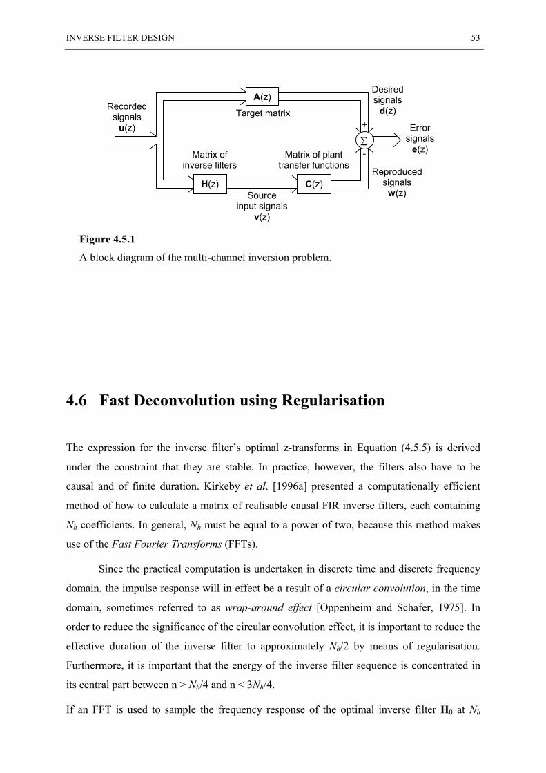
INVERSE FILTER DESIGN 53
Figure 4.5.1
A block diagram of the multi-channel inversion problem.
4.6 Fast Deconvolution using Regularisation
The expression for the inverse filter’s optimal z-transforms in Equation (4.5.5) is derived
under the constraint that they are stable. In practice, however, the filters also have to be
causal and of finite duration. Kirkeby et al. [1996a] presented a computationally efficient
method of how to calculate a matrix of realisable causal FIR inverse filters, each containing
Nh coefficients. In general, Nh must be equal to a power of two, because this method makes
use of the Fast Fourier Transforms (FFTs).
Since the practical computation is undertaken in discrete time and discrete frequency
domain, the impulse response will in effect be a result of a circular convolution, in the time
domain, sometimes referred to as wrap-around effect [Oppenheim and Schafer, 1975]. In
order to reduce the significance of the circular convolution effect, it is important to reduce the
effective duration of the inverse filter to approximately Nh/2 by means of regularisation.
Furthermore, it is important that the energy of the inverse filter sequence is concentrated in
its central part between n > Nh/4 and n < 3Nh/4.
If an FFT is used to sample the frequency response of the optimal inverse filter H0 at Nh
Recordedsignals
u(z)
H(z)Source
input signalsv(z)
Reproducedsignals
w(z)
A(z)
C(z)
∑-
+
Desiredsignals
d(z)
Errorsignals
e(z)
Target matrix
Matrix ofinverse filters
Matrix of planttransfer functions
INVERSE FILTER DESIGN 54
points around the unit circle, then the value of H0(k) at those frequencies is given by
)()(])()([)( 10 kkβkkk HH ACICCH −+= ,
(4.6.1)
where k denotes the k’th frequency line, that is the frequency corresponding to the complex
number exp(j2πk/Nh). The superscript H stands for the Hermitian operator which transposes
and conjugates its argument [Nelson and Elliott, 1992, Appendix A]. Consequently, the
generalised crosstalk cancellation matrix, according to Equation (4.5.6), is given by
)(])()([)( 1I kβkkk HH CICCH −+= .
(4.6.2)
Thus, for the practical implementation of the algorithm in order to calculate the impulse
responses of the inverse filters hI(n), the following steps are necessary:
1. Calculate C(k) by taking [R × S] Nh-point FFTs of the plant impulse responses crs(n).
2. For each of the Nh values of k, calculate the [S × R] matrix HI(k) from Equation (4.6.2).
3. Calculate hI(n) by taking [S × R] Nh-point inverse FFTs of the elements of HI(k) followed
by a cyclic shift of Nh/2 points in order to implement the modelling delay.
It should be mentioned that this method, referred to as “fast deconvolution”, is
typically several hundred times faster than a conventional time domain steepest descent
algorithm. However, this frequency domain method requires relatively long inverse filters.
Thus, it should be used only when hardware- or memory restrictions are not too severe. It is
necessary to set the regularisation parameter β to an appropriate value, but the ecaxt value of
β is usually not critical, and can be determined by a few trial-and-error experiments.
4.7 Ill-conditioning and the effect of regularisation
INVERSE FILTER DESIGN 55
As described in the previous sections, the whole physical process of inverse filtering is
solved numerically by means of equation systems which are usually cast into matrix form.
From matrix algebra, it is well known that the inverse of a matrix C can be calculated only
when C is not singular, i.e., its determinant is not zero. Any [R × S] matrix C can be
factorised into a product of three matrices U, Σ, and VH, such as
H1
H VUVΣUC
==
Sσ
σO ,
(4.7.1)
where U and V are orthonormal. Σ is a diagonal matrix containing the singular values σS of
C where σ1 ≥ σ2 ≥ ... ≥ σS. Therefore, Equation (4.7.1) is called the singular value
decomposition of C [Bronstein and Semendjajew, 1996], which illustrates some important
properties of linear equation systems. The singular values are defined as the square roots of
the eigenvalues of CHC, and since CHC is Hermitian, they are always real and positive
[Kreyszig, 1983].
If Σ contains a singular value of zero, the matrix C does not have full rank, i.e., there
is a linear dependence between its columns. In that case, the matrix C is said to be singular
and, consequently, its inversion does not exist. If C is not singular, its exact inverse is given
by
[ ] H1
H11H1 1
1 UVUΣVVΣUC
=== −−−
Sσ
σO .
(4.7.2)
In theory, a singular value is either zero or not zero, but when singular values are
calculated by a numerical algorithm, a true singular value of zero will usually come out as a
very small number [Press et al., 1992]. Similarly, if the equations are close to being linearly
dependent, but without being exactly linearly dependent, they will also result in a very small
singular value. A very small singular value σS makes the corresponding element 1/σS in Σ-1
very large. This phenomenon is called ill-conditioning, and it is usually undesirable because
it makes the solution very sensitive to small changes in the data.
A quantifier of the ill-conditioning problem is the so-called condition number,

INVERSE FILTER DESIGN 56
sometimes referred to as the spectral condition number [Wilkinson, 1965], which is defined
as the ratio between the maximum and the minimum singular value of C,
min
max)κ(σσ
=C .
(4.7.3)
A well-conditioned matrix has a condition number close to one, while an ill-conditioned
matrix has a large condition number.
Considering the crosstalk cancellation problem for a typical two channel sound
reproduction system, as it was applied in the present work, C(ω) is a [2 × 2] matrix of
electro-acoustic transfer functions between the two loudspeakers and the two microphones or
ears. For the arrangement given in Figure 3.4.1 and according to Equation 3.4.1, ill-
conditioning will occur for the following situations:
1. CLL(ω) = CRL(ω) = 0 or CRR(ω) = CLR(ω) = 0. This occurs when all transfer functions from
all loudspeakers to any of the microphones are zeros at the same frequency, leading to a
zero row in the matrix C(ω). In practice, this may happen when the frequency responses
of all loudspeakers have a notch at the same frequency, or the concerned microphone is
insensitive at a certain frequency.
2. CLL(ω) = CLR(ω) = 0 or CRR(ω) = CRL(ω) = 0. This occurs when all transfer functions from
any of the loudspeakers to all microphones are zeros at the same frequency, leading to a
zero column in the matrix C(ω). Similar practical causes as those mentioned above may
also be valid in this case.
3. CLL(ω)⋅CRR(ω) = CLR(ω)⋅CRL(ω). This situation occurs in special symmetrical acoustic
arrangements. For example, at low frequencies, the difference between the direct and the
crosstalk path length is very small compared to the wavelength. Therefore, all four
transfer functions show maximum similarity between each other, which leads to ill-
conditioning. This explains the particular difficulties of crosstalk cancellation systems at
low frequencies as mentioned in Section 3.4.
For the case of the crosstalk cancellation problem, ill-conditioning is undesirable

INVERSE FILTER DESIGN 57
since it tends to make the inverse filter’s output signals v very large. These signals in turn
represent the input signals to audio amplifiers which drive the reproduction loudspeakers of
the system. Thus, without any precautions, the inverse filters would excessively amplify the
ill-conditioned frequencies, which likely leads to saturation of the audio amplifiers and/or
damage of the loudspeakers.
If regularisation is applied to the system inversion, the optimal solution for the inverse
filters will be forced to a lower power output, as discussed in Section 4.4. Thus, by setting β
to an appropriate value it can be ensured that the system does not boost any ill-conditioned
frequencies to much. In other words, by means of the regularisation parameter β, it can be
exactly specified how “non-singular” the plant matrix C should be.
Chapter 5 Optimal Source Distribution
5.1 Introduction
As discussed in the previous chapter, the problem of ill-conditioning leads to a lack of
robustness of the system inversion involved with crosstalk cancellation. Moreover, the
system inversion requires amplification of the signal at certain frequencies and attenuation of
the signal at other frequencies. This amplification directly results in a loss of dynamic range
of the system. The technique of regularisation allows to reduce both dynamic range loss and
the sensitivity to small errors around ill-conditioned frequencies.
In general, as already indicated in Section 4.7, the conditioning of a system depends
on frequency and on the positions of the reproduction loudspeakers relative to the
microphones (ears). Investigations of the problem with respect to frequency and the system’s
geometry were undertaken by Takeuchi and Nelson [2000a; 2000b]. Thereby, based on an
analysis of a free field model of the system, it was shown that if one were able to vary the
loudspeaker span as a function of frequency, the problems of loss of dynamic range and
robustness, could be ideally solved. This idea has resulted in the proposal of a new system,
referred to as the “Optimal Source Distribution” or “OSD” system, by Takeuchi and Nelson
[2000a; 2000b]. In the present work, such a system was put into practice and its performance
investigated. Therefore, based on the publications of Takeuchi and Nelson [2000a; 2000b],
the essential points in the theory and the idea behind the „OSD“ system as well as practical
design considerations will be described in this chapter.
5.2 Free field model of the system
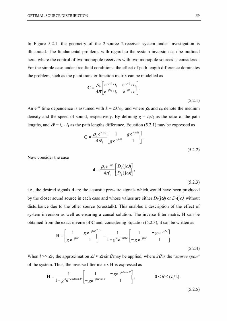
OPTIMAL SOURCE DISTRIBUTION 59
In Figure 5.2.1, the geometry of the 2-source 2-receiver system under investigation is
illustrated. The fundamental problems with regard to the system inversion can be outlined
here, where the control of two monopole receivers with two monopole sources is considered.
For the simple case under free field conditions, the effect of path length difference dominates
the problem, such as the plant transfer function matrix can be modelled as
= −−
−−
1j
2j
2j
1j
0
/e/e/e/e
4 12
21
llll
klkl
klkl
πρ
C ,
(5.2.1)
An ejωt time dependence is assumed with k = ω /c0, and where ρ0 and c0 denote the medium
density and the speed of sound, respectively. By defining g = l1/l2 as the ratio of the path
lengths, and ∆l = l2 - l1 as the path lengths difference, Equation (5.2.1) may be expressed as
=
∆−
∆−−
1ee1
4e
j
j
1
j0
1
lk
lkkl
gg
lπρ
C .
(5.2.2)
Now consider the case
=
−
)j()j(
4e
2
1
1
j0
1
ωω
πρ
DD
l
kl
d ,
(5.2.3)
i.e., the desired signals d are the acoustic pressure signals which would have been produced
by the closer sound source in each case and whose values are either D1(jω) or D2(jω) without
disturbance due to the other source (crosstalk). This enables a description of the effect of
system inversion as well as ensuring a causal solution. The inverse filter matrix H can be
obtained from the exact inverse of C and, considering Equation (5.2.3), it can be written as
−−
−=
=
∆−
∆−
∆−
−
∆−
∆−
1ee1
e11
1ee1
j
j
2j2
1
j
j
lk
lk
lklk
lk
gg
ggg
H .
(5.2.4)
When l >> ∆r, the approximation ∆l ≈ ∆rsinθ may be applied, where 2θ is the “source span”
of the system. Thus, the inverse filter matrix H is expressed as
−−
−=
∆−
∆−
∆− 1ee1
e11
sinrj
sinrj
sinr2j2 θ
θ
θ k
k
k gg
gH , )2(0 πθ ≤< .
(5.2.5)
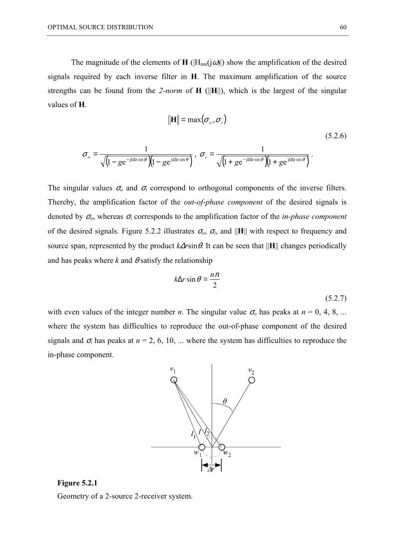
OPTIMAL SOURCE DISTRIBUTION 60
The magnitude of the elements of H (|Hmn(jω)|) show the amplification of the desired
signals required by each inverse filter in H. The maximum amplification of the source
strengths can be found from the 2-norm of H (||H||), which is the largest of the singular
values of H.
( )io σσ ,max=H
(5.2.6)
( )( )θθσ
sinrjsinrj e1e11
∆∆− −−=
kkogg
, ( )( )θθσ
sinrjsinrj e1e11
∆∆− ++=
kkigg
.
The singular values σo and σi correspond to orthogonal components of the inverse filters.
Thereby, the amplification factor of the out-of-phase component of the desired signals is
denoted by σo, whereas σi corresponds to the amplification factor of the in-phase component
of the desired signals. Figure 5.2.2 illustrates σo, σi, and ||H|| with respect to frequency and
source span, represented by the product k∆rsinθ. It can be seen that ||H|| changes periodically
and has peaks where k and θ satisfy the relationship
2sin πθ nrk =∆
(5.2.7)
with even values of the integer number n. The singular value σo has peaks at n = 0, 4, 8, ...
where the system has difficulties to reproduce the out-of-phase component of the desired
signals and σi has peaks at n = 2, 6, 10, ... where the system has difficulties to reproduce the
in-phase component.
Figure 5.2.1
Geometry of a 2-source 2-receiver system.
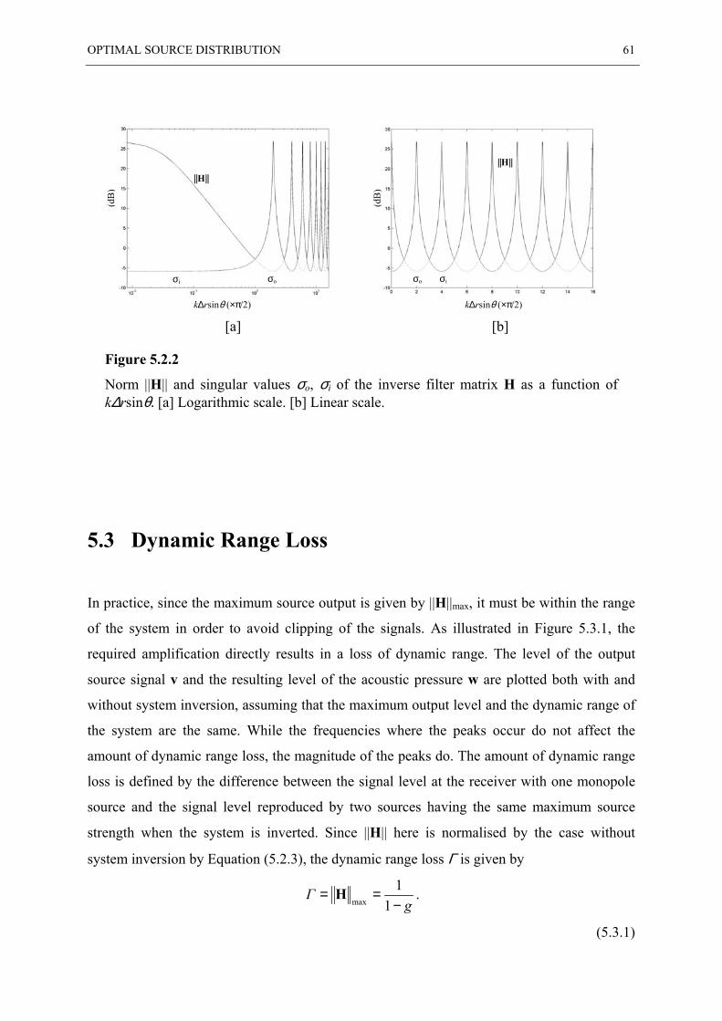
OPTIMAL SOURCE DISTRIBUTION 61
[a] [b]
Figure 5.2.2
Norm ||H|| and singular values σo, σi of the inverse filter matrix H as a function ofk∆rsinθ. [a] Logarithmic scale. [b] Linear scale.
5.3 Dynamic Range Loss
In practice, since the maximum source output is given by ||H||max, it must be within the range
of the system in order to avoid clipping of the signals. As illustrated in Figure 5.3.1, the
required amplification directly results in a loss of dynamic range. The level of the output
source signal v and the resulting level of the acoustic pressure w are plotted both with and
without system inversion, assuming that the maximum output level and the dynamic range of
the system are the same. While the frequencies where the peaks occur do not affect the
amount of dynamic range loss, the magnitude of the peaks do. The amount of dynamic range
loss is defined by the difference between the signal level at the receiver with one monopole
source and the signal level reproduced by two sources having the same maximum source
strength when the system is inverted. Since ||H|| here is normalised by the case without
system inversion by Equation (5.2.3), the dynamic range loss Γ is given by
gΓ
−==
11
maxH .
(5.3.1)
||H||
σi σo
||H||
k∆rsinθ (×π/2)
(dB
)
k∆rsinθ (×π/2)
σiσo
(dB
)
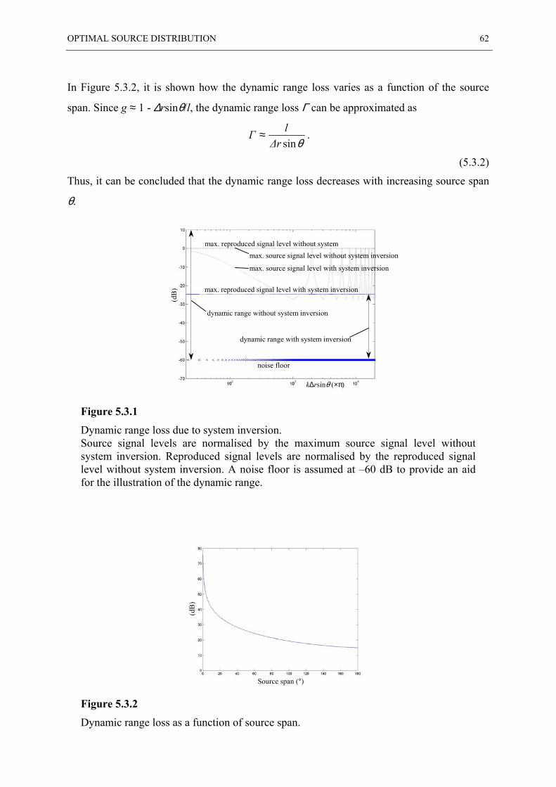
OPTIMAL SOURCE DISTRIBUTION 62
In Figure 5.3.2, it is shown how the dynamic range loss varies as a function of the source
span. Since g ≈ 1 - ∆rsinθ/l, the dynamic range loss Γ can be approximated as
θsin∆rlΓ ≈ .
(5.3.2)
Thus, it can be concluded that the dynamic range loss decreases with increasing source span
θ.
Figure 5.3.1
Dynamic range loss due to system inversion.Source signal levels are normalised by the maximum source signal level withoutsystem inversion. Reproduced signal levels are normalised by the reproduced signallevel without system inversion. A noise floor is assumed at –60 dB to provide an aidfor the illustration of the dynamic range.
Figure 5.3.2
Dynamic range loss as a function of source span.
Source span (°)
(dB
)
max. reproduced signal level without system
max. reproduced signal level with system inversion
dynamic range without system inversion
dynamic range with system inversion
noise floor
max. source signal level without system inversion
max. source signal level with system inversion
k∆rsinθ (×π)
(dB
)
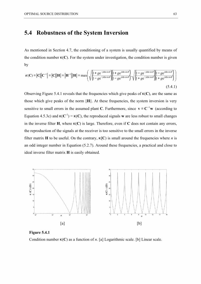
OPTIMAL SOURCE DISTRIBUTION 63
5.4 Robustness of the System Inversion
As mentioned in Section 4.7, the conditioning of a system is usually quantified by means of
the condition number κ(C). For the system under investigation, the condition number is given
by
( )( )( )( )
( )( )( )( )
++−−
−−++==== ∆∆−
∆∆−
∆∆−
∆∆−−−
θθ
θθ
θθ
θθ
κ sinrjsinrj
sinrjsinrj
sinrjsinrj
sinrjsinrj11
e1e1e1e1,
e1e1e1e1max)( kk
kk
kk
kk
gggg
ggggHHHCCCC
(5.4.1)
Observing Figure 5.4.1 reveals that the frequencies which give peaks of κ(C), are the same as
those which give peaks of the norm ||H||. At these frequencies, the system inversion is very
sensitive to small errors in the assumed plant C. Furthermore, since wCv 1−= (according to
Equation 4.5.3c) and κ(C-1) = κ(C), the reproduced signals w are less robust to small changes
in the inverse filter H, where κ(C) is large. Therefore, even if C does not contain any errors,
the reproduction of the signals at the receiver is too sensitive to the small errors in the inverse
filter matrix H to be useful. On the contrary, κ(C) is small around the frequencies where n is
an odd integer number in Equation (5.2.7). Around these frequencies, a practical and close to
ideal inverse filter matrix H is easily obtained.
[a] [b]
Figure 5.4.1
Condition number κ(C) as a function of n. [a] Logarithmic scale. [b] Linear scale.
κ (C
) (dB
)
κ(C
) (d
B)
nn
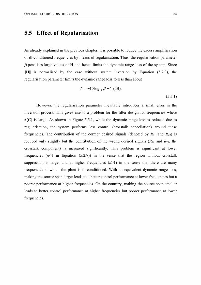
OPTIMAL SOURCE DISTRIBUTION 64
5.5 Effect of Regularisation
As already explained in the previous chapter, it is possible to reduce the excess amplification
of ill-conditioned frequencies by means of regularisation. Thus, the regularisation parameter
β penalises large values of H and hence limits the dynamic range loss of the system. Since
||H|| is normalised by the case without system inversion by Equation (5.2.3), the
regularisation parameter limits the dynamic range loss to less than about
6log10 10 −−≈ βΓ (dB).
(5.5.1)
However, the regularisation parameter inevitably introduces a small error in the
inversion process. This gives rise to a problem for the filter design for frequencies where
κ(C) is large. As shown in Figure 5.5.1, while the dynamic range loss is reduced due to
regularisation, the system performs less control (crosstalk cancellation) around these
frequencies. The contribution of the correct desired signals (denoted by R11 and R22) is
reduced only slightly but the contribution of the wrong desired signals (R12 and R21, the
crosstalk component) is increased significantly. This problem is significant at lower
frequencies (n<1 in Equation (5.2.7)) in the sense that the region without crosstalk
suppression is large, and at higher frequencies (n>1) in the sense that there are many
frequencies at which the plant is ill-conditioned. With an equivalent dynamic range loss,
making the source span larger leads to a better control performance at lower frequencies but a
poorer performance at higher frequencies. On the contrary, making the source span smaller
leads to better control performance at higher frequencies but poorer performance at lower
frequencies.
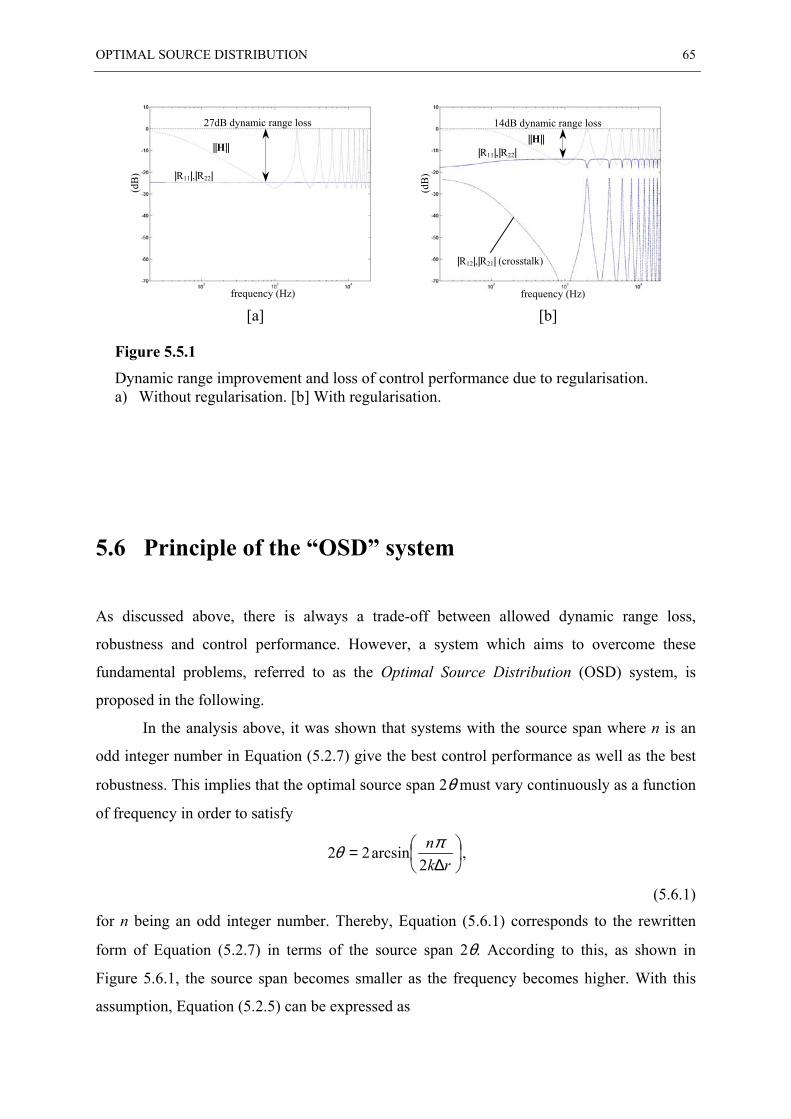
OPTIMAL SOURCE DISTRIBUTION 65
[a] [b]
Figure 5.5.1
Dynamic range improvement and loss of control performance due to regularisation.a) Without regularisation. [b] With regularisation.
5.6 Principle of the “OSD” system
As discussed above, there is always a trade-off between allowed dynamic range loss,
robustness and control performance. However, a system which aims to overcome these
fundamental problems, referred to as the Optimal Source Distribution (OSD) system, is
proposed in the following.
In the analysis above, it was shown that systems with the source span where n is an
odd integer number in Equation (5.2.7) give the best control performance as well as the best
robustness. This implies that the optimal source span 2θ must vary continuously as a function
of frequency in order to satisfy
∆=
rkn
2arcsin22 πθ ,
(5.6.1)
for n being an odd integer number. Thereby, Equation (5.6.1) corresponds to the rewritten
form of Equation (5.2.7) in terms of the source span 2θ. According to this, as shown in
Figure 5.6.1, the source span becomes smaller as the frequency becomes higher. With this
assumption, Equation (5.2.5) can be expressed as
27dB dynamic range loss
|R11|,|R22|
||H||
frequency (Hz)
(dB
)14dB dynamic range loss
|R11|,|R22|||H||
frequency (Hz)
(dB
)
|R12|,|R21| (crosstalk)
OPTIMAL SOURCE DISTRIBUTION 66
H =+
−−
11
112gg
gj
j.
(5.6.2)
Note that H = 1 2 and κ(C) = 1 for all frequencies. Therefore, there is no dynamic range
loss compared to the case without system inversion. In fact, the dynamic range is gained by
3dB since the two orthogonal components of the desired signals are π/2 out of phase. The
error in calculating the inverse filter is small and the system has very good control over the
reproduced signals. The system is also very robust to changes in the plant matrix.
According to Equation (5.6.1), the range of source span is given by the frequency
range of interest. In Figure 5.6.1 it can be seen that a smaller value of n gives a smaller
source span for the same frequency. Therefore, the smallest source span 2θh for the same
high frequency limit is given by n = 1. This value is about 8° to give optimal control of the
sound field at two positions separated by the distance between two ears (about 0.13m for a
KEMAR dummy head) up to a frequency of 20kHz.
Equation (5.2.7) can also be rewritten in terms of frequency as
θsin40
∆rnc
f = .
(5.6.3)
The smallest value of n gives the lowest frequency limit for a given source span. Because
sinθ ≤ 1,
∆rnc
f4
0≥ ,
(5.6.4)
i.e., the physically maximum source span of 2θ = 180° gives the low frequency limit fl.
Obviously, the lowest low frequency limit is given by n = 1. For a system designed to control
the sound field at the two ear positions, this value is about fl = 300 ~ 400 Hz.
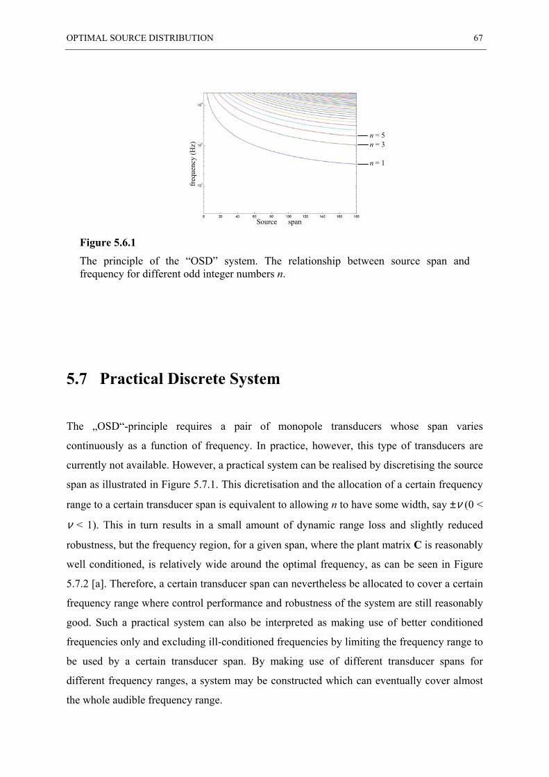
OPTIMAL SOURCE DISTRIBUTION 67
Figure 5.6.1
The principle of the “OSD” system. The relationship between source span andfrequency for different odd integer numbers n.
5.7 Practical Discrete System
The „OSD“-principle requires a pair of monopole transducers whose span varies
continuously as a function of frequency. In practice, however, this type of transducers are
currently not available. However, a practical system can be realised by discretising the source
span as illustrated in Figure 5.7.1. This dicretisation and the allocation of a certain frequency
range to a certain transducer span is equivalent to allowing n to have some width, say ±ν (0 <
ν < 1). This in turn results in a small amount of dynamic range loss and slightly reduced
robustness, but the frequency region, for a given span, where the plant matrix C is reasonably
well conditioned, is relatively wide around the optimal frequency, as can be seen in Figure
5.7.2 [a]. Therefore, a certain transducer span can nevertheless be allocated to cover a certain
frequency range where control performance and robustness of the system are still reasonably
good. Such a practical system can also be interpreted as making use of better conditioned
frequencies only and excluding ill-conditioned frequencies by limiting the frequency range to
be used by a certain transducer span. By making use of different transducer spans for
different frequency ranges, a system may be constructed which can eventually cover almost
the whole audible frequency range.
n = 1
n = 3n = 5
freq
uenc
y (H
z)
Source span
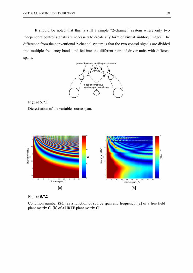
OPTIMAL SOURCE DISTRIBUTION 68
It should be noted that this is still a simple “2-channel” system where only two
independent control signals are necessary to create any form of virtual auditory images. The
difference from the conventional 2-channel system is that the two control signals are divided
into multiple frequency bands and fed into the different pairs of driver units with different
spans.
Figure 5.7.1
Dicretisation of the variable source span.
[a] [b]
Figure 5.7.2
Condition number κ(C) as a function of source span and frequency. [a] of a free fieldplant matrix C. [b] of a HRTF plant matrix C.
Source span (°)
freq
uenc
y (H
z)
(dB
)
Source span (°)
freq
uenc
y (H
z)
(dB
)
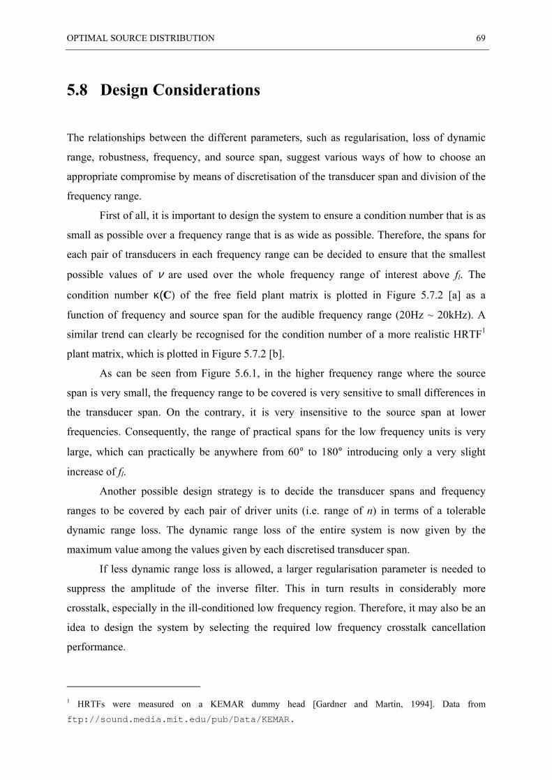
OPTIMAL SOURCE DISTRIBUTION 69
5.8 Design Considerations
The relationships between the different parameters, such as regularisation, loss of dynamic
range, robustness, frequency, and source span, suggest various ways of how to choose an
appropriate compromise by means of discretisation of the transducer span and division of the
frequency range.
First of all, it is important to design the system to ensure a condition number that is as
small as possible over a frequency range that is as wide as possible. Therefore, the spans for
each pair of transducers in each frequency range can be decided to ensure that the smallest
possible values of ν are used over the whole frequency range of interest above fl. The
condition number κ(C) of the free field plant matrix is plotted in Figure 5.7.2 [a] as a
function of frequency and source span for the audible frequency range (20Hz ~ 20kHz). A
similar trend can clearly be recognised for the condition number of a more realistic HRTF1
plant matrix, which is plotted in Figure 5.7.2 [b].
As can be seen from Figure 5.6.1, in the higher frequency range where the source
span is very small, the frequency range to be covered is very sensitive to small differences in
the transducer span. On the contrary, it is very insensitive to the source span at lower
frequencies. Consequently, the range of practical spans for the low frequency units is very
large, which can practically be anywhere from 60° to 180° introducing only a very slight
increase of fl.
Another possible design strategy is to decide the transducer spans and frequency
ranges to be covered by each pair of driver units (i.e. range of n) in terms of a tolerable
dynamic range loss. The dynamic range loss of the entire system is now given by the
maximum value among the values given by each discretised transducer span.
If less dynamic range loss is allowed, a larger regularisation parameter is needed to
suppress the amplitude of the inverse filter. This in turn results in considerably more
crosstalk, especially in the ill-conditioned low frequency region. Therefore, it may also be an
idea to design the system by selecting the required low frequency crosstalk cancellation
performance.
1 HRTFs were measured on a KEMAR dummy head [Gardner and Martin, 1994]. Data fromftp://sound.media.mit.edu/pub/Data/KEMAR.
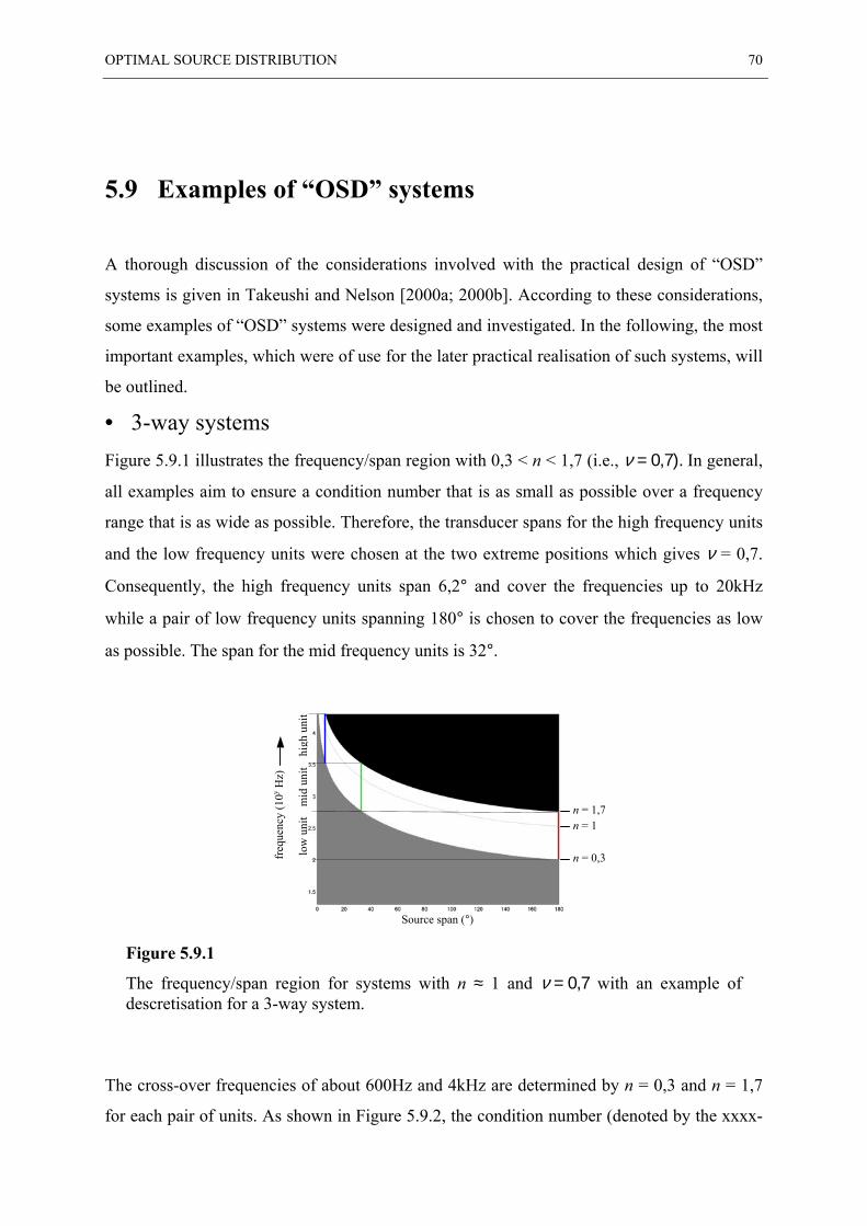
OPTIMAL SOURCE DISTRIBUTION 70
5.9 Examples of “OSD” systems
A thorough discussion of the considerations involved with the practical design of “OSD”
systems is given in Takeushi and Nelson [2000a; 2000b]. According to these considerations,
some examples of “OSD” systems were designed and investigated. In the following, the most
important examples, which were of use for the later practical realisation of such systems, will
be outlined.
• 3-way systemsFigure 5.9.1 illustrates the frequency/span region with 0,3 < n < 1,7 (i.e., ν = 0,7). In general,
all examples aim to ensure a condition number that is as small as possible over a frequency
range that is as wide as possible. Therefore, the transducer spans for the high frequency units
and the low frequency units were chosen at the two extreme positions which gives ν = 0,7.
Consequently, the high frequency units span 6,2° and cover the frequencies up to 20kHz
while a pair of low frequency units spanning 180° is chosen to cover the frequencies as low
as possible. The span for the mid frequency units is 32°.
Figure 5.9.1
The frequency/span region for systems with n ≈ 1 and ν = 0,7 with an example ofdescretisation for a 3-way system.
The cross-over frequencies of about 600Hz and 4kHz are determined by n = 0,3 and n = 1,7
for each pair of units. As shown in Figure 5.9.2, the condition number (denoted by the xxxx-
n = 0,3
n = 1n = 1,7
low
uni
thi
gh u
nit
mid
uni
t
freq
uenc
y (1
0y Hz)
Source span (°)
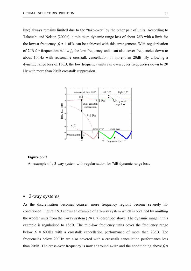
OPTIMAL SOURCE DISTRIBUTION 71
line) always remains limited due to the “take-over” by the other pair of units. According to
Takeuchi and Nelson [2000a], a minimum dynamic range loss of about 7dB with a limit for
the lowest frequency fl ≈ 110Hz can be achieved with this arrangement. With regularisation
of 7dB for frequencies below fl, the low frequency units can also cover frequencies down to
about 100Hz with reasonable crosstalk cancellation of more than 20dB. By allowing a
dynamic range loss of 13dB, the low frequency units can even cover frequencies down to 20
Hz with more than 20dB crosstalk suppression.
Figure 5.9.2
An example of a 3-way system with regularisation for 7dB dynamic range loss.
• 2-way systemsAs the discretisation becomes coarser, more frequency regions become severely ill-
conditioned. Figure 5.9.3 shows an example of a 2-way system which is obtained by omitting
the woofer units from the 3-way system (ν ≈ 0.7) described above. The dynamic range in this
example is regularised to 18dB. The mid-low frequency units cover the frequency range
below fl ≈ 600Hz with a crosstalk cancellation performance of more than 20dB. The
frequencies below 200Hz are also covered with a crosstalk cancellation performance less
than 20dB. The cross-over frequency is now at around 4kHz and the conditioning above fl ≈
|R11|, |R22|
|R12|, |R21|
sub-low & low: 180° mid: 32°
7dB dynamicrange loss
crosstalk limit fl
||H||
20dB crosstalksuppression
frequency (Hz)
κ(C)
||H||,
|Rm
n| (d
B)
high: 6,2°
cross-overcross-over
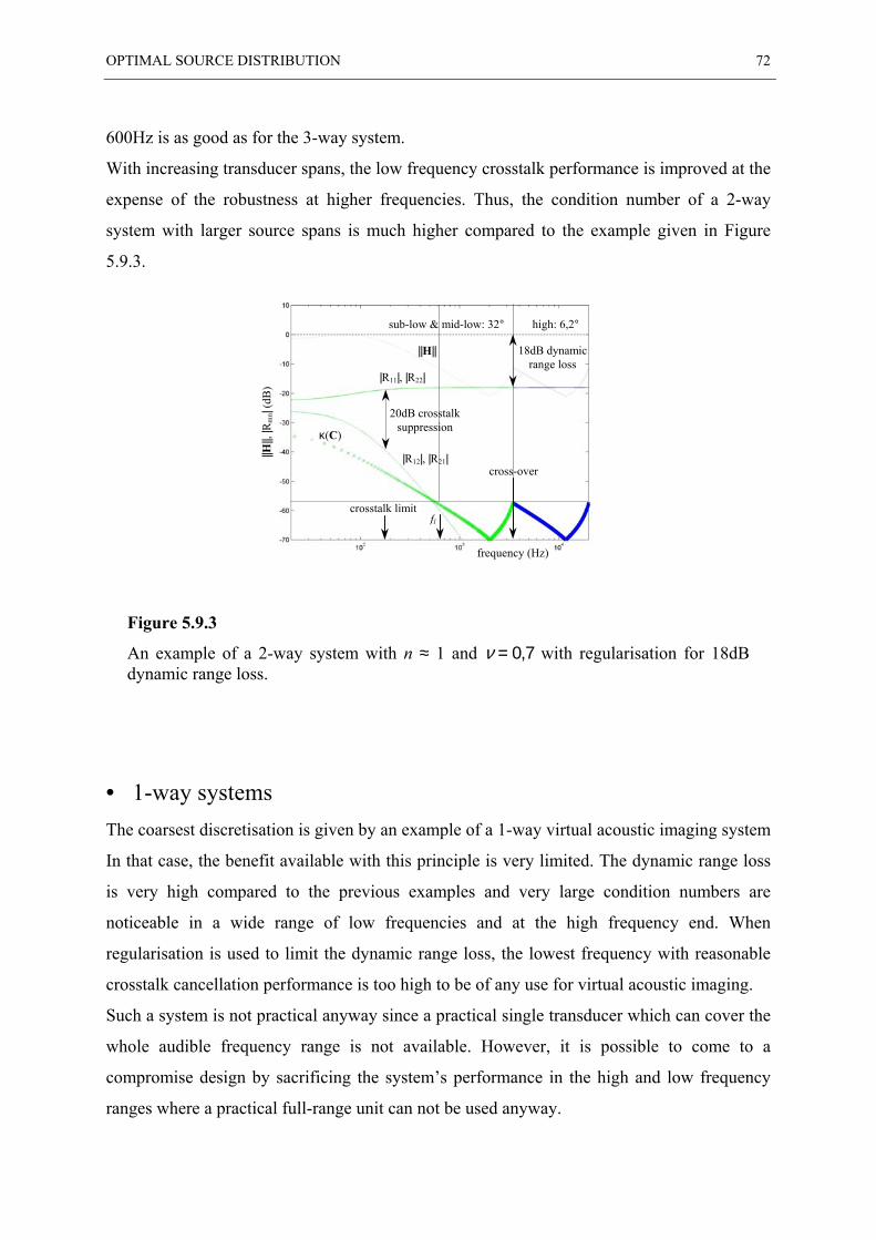
OPTIMAL SOURCE DISTRIBUTION 72
600Hz is as good as for the 3-way system.
With increasing transducer spans, the low frequency crosstalk performance is improved at the
expense of the robustness at higher frequencies. Thus, the condition number of a 2-way
system with larger source spans is much higher compared to the example given in Figure
5.9.3.
Figure 5.9.3
An example of a 2-way system with n ≈ 1 and ν = 0,7 with regularisation for 18dBdynamic range loss.
• 1-way systemsThe coarsest discretisation is given by an example of a 1-way virtual acoustic imaging system
In that case, the benefit available with this principle is very limited. The dynamic range loss
is very high compared to the previous examples and very large condition numbers are
noticeable in a wide range of low frequencies and at the high frequency end. When
regularisation is used to limit the dynamic range loss, the lowest frequency with reasonable
crosstalk cancellation performance is too high to be of any use for virtual acoustic imaging.
Such a system is not practical anyway since a practical single transducer which can cover the
whole audible frequency range is not available. However, it is possible to come to a
compromise design by sacrificing the system’s performance in the high and low frequency
ranges where a practical full-range unit can not be used anyway.
|R11|, |R22|
|R12|, |R21|
sub-low & mid-low: 32° high: 6,2°
18dB dynamicrange loss
crosstalk limitfl
||H||
20dB crosstalksuppression
frequency (Hz)
κ(C)
||H||,
|Rm
n| (d
B)
cross-over
OPTIMAL SOURCE DISTRIBUTION 73
• “Multi-region” systemsIt is also possible to compromise further by utilising two or more regions of n. This approach
is beneficial when one attempts to cover a wider frequency range with a smaller number of
transducer pairs. The “Stereo Dipole” system [Kirkeby et al., 1996b], which uses a source
span of 10°, is such a system. The simplest case with a single pair of transducers is when the
regions of 0 < n < 2 and 2 < n < 4 are utilised. In that case, the cross-talk cancellation
performance in the low frequency range is improved compared to a 1-way system described
above. However, the system makes also use of the region where n = 2 (even). Thus, the
system has little control and is not robust at the frequencies corresponding to this (unusable)
region of n.
5.10 Inverse filtering when using cross-over filters
In order to distribute the frequencies of the signal to the appropriate pair of driver units,
cross-over filters (low pass, high pass or band pass filters) have to be applied to the “OSD”
system. Since an ideal filter which gives a rectangular window in the frequency domain can
not be realised in practice, there are frequency regions around the cross-over frequency where
multiple pairs of driver units are contributing to the synthesis of the reproduced signals w.
Therefore, it is important to ensure that this transition region is also within the well-
conditioned region of the principle.
For the practical design, the plant matrix C of the system needs to be known in order
to enable an appropriate inverse filtering for the crosstalk cancellation. The most obvious
way of obtaining C is when the cross-over network is included in the measurements, as it is
illustrated for a 2-way system in Figure 5.10.1. In this case, the plant C consists of a single [2
× 2] matrix of electro-acoustic transfer functions and the obtained inverse filter matrix H
automatically compensates for the response of the cross-over network and the interaction
OPTIMAL SOURCE DISTRIBUTION 74
between different pairs of driver units around the cross-over frequency.
Alternatively, one can design m inverse filter matrices H1, H2, ... Hm for plants C1, C2,
... Cm of m pairs of driver units (Figure 5.10.2). In this case, around cross-over frequencies, a
virtual acoustic environment is synthesised with two adjacent inverse filter matrices.
Provided the cross-over filters behave well, the correct desired signals are reproduced as a
simple sum of the two involved desired signals. Since the system inversion is now
independent of the cross-over filters, the cross-over filters can be applied both after and prior
to the inverse filters.
It is also possible to obtain a [2 × 2m] plant matrix C, between each driver unit and
the two ears separately, where m is the number of driver pairs (Figure 5.10.3).
The system is now underdetermined and a [2m × 2] pseudo inverse filter matrix H is given by
[ ]H C CC I= +−H H 1
β .
(5.10.1)
This solution ensures that the least effort (smallest output) of the transducers is used in
providing the desired signals at the listener’s ears. The net result is similar to the case with a
single [2 × 2] plant matrix inversion described above.
When the cross-over filters are omitted, the problem becomes a conventional multi-
channel system, contrary to the “OSD” system which is a multi-way system. In this case, the
plant matrix is again of dimension [2 × 2m] where 2m is the number of channels. The [2m ×
2] pseudo inverse filter matrix H given by Equation (5.10.1) automatically distributes the
signal to different drivers so that least effort is required. This property is beneficial since ill-
conditioned frequencies and HRTF-minima are automatically avoided. On the other hand,
with the absence of the cross-over filters, multi-channel systems do not have some of the
merit of the “OSD” system. Even though the inversion of multi-channel systems ensures that
most of the lower frequency signals are distributed to the pair of units with larger span
(woofers), some of the higher frequency signals are also distributed to the woofers. This is
because due to its periodic nature there are a number of frequencies for which the larger span
gives a smaller condition number. This in turn requires the woofers to produce a very wide
frequency range of signals, which is not practical. Another merit of the “OSD” system is also
lost in a multi-channel system. That is to say that only two independent output signals, hence
only two amplifier channels, are required for a “OSD” system whereas the same number of
channels as the number of driver units are always required for a multi-channel system.
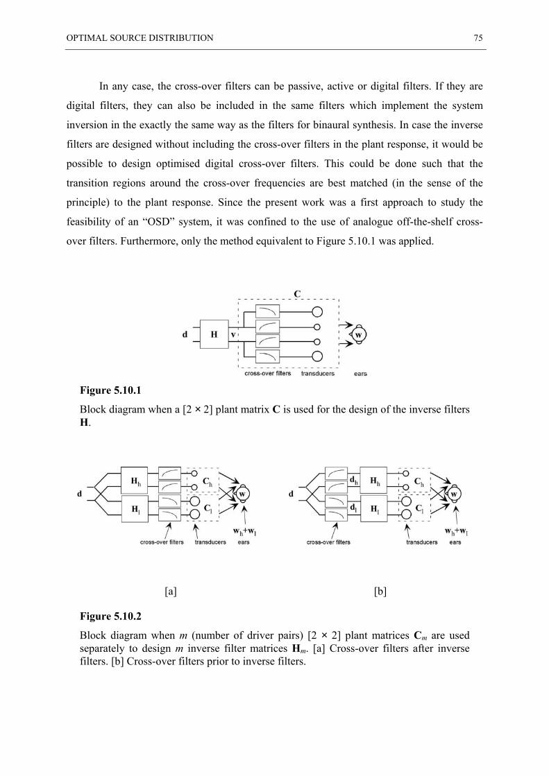
OPTIMAL SOURCE DISTRIBUTION 75
In any case, the cross-over filters can be passive, active or digital filters. If they are
digital filters, they can also be included in the same filters which implement the system
inversion in the exactly the same way as the filters for binaural synthesis. In case the inverse
filters are designed without including the cross-over filters in the plant response, it would be
possible to design optimised digital cross-over filters. This could be done such that the
transition regions around the cross-over frequencies are best matched (in the sense of the
principle) to the plant response. Since the present work was a first approach to study the
feasibility of an “OSD” system, it was confined to the use of analogue off-the-shelf cross-
over filters. Furthermore, only the method equivalent to Figure 5.10.1 was applied.
Figure 5.10.1
Block diagram when a [2 × 2] plant matrix C is used for the design of the inverse filtersH.
[a] [b]
Figure 5.10.2
Block diagram when m (number of driver pairs) [2 × 2] plant matrices Cm are usedseparately to design m inverse filter matrices Hm. [a] Cross-over filters after inversefilters. [b] Cross-over filters prior to inverse filters.
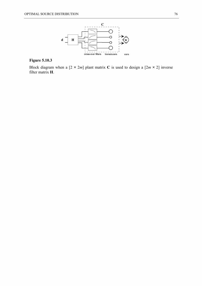
OPTIMAL SOURCE DISTRIBUTION 76
Figure 5.10.3
Block diagram when a [2 × 2m] plant matrix C is used to design a [2m × 2] inversefilter matrix H.
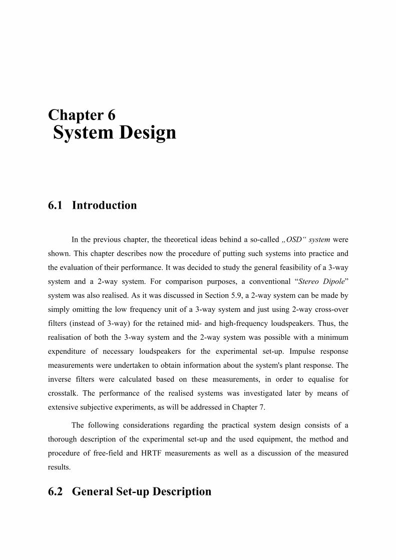
Chapter 6 System Design
6.1 Introduction
In the previous chapter, the theoretical ideas behind a so-called „OSD“ system were
shown. This chapter describes now the procedure of putting such systems into practice and
the evaluation of their performance. It was decided to study the general feasibility of a 3-way
system and a 2-way system. For comparison purposes, a conventional “Stereo Dipole”
system was also realised. As it was discussed in Section 5.9, a 2-way system can be made by
simply omitting the low frequency unit of a 3-way system and just using 2-way cross-over
filters (instead of 3-way) for the retained mid- and high-frequency loudspeakers. Thus, the
realisation of both the 3-way system and the 2-way system was possible with a minimum
expenditure of necessary loudspeakers for the experimental set-up. Impulse response
measurements were undertaken to obtain information about the system's plant response. The
inverse filters were calculated based on these measurements, in order to equalise for
crosstalk. The performance of the realised systems was investigated later by means of
extensive subjective experiments, as will be addressed in Chapter 7.
The following considerations regarding the practical system design consists of a
thorough description of the experimental set-up and the used equipment, the method and
procedure of free-field and HRTF measurements as well as a discussion of the measured
results.
6.2 General Set-up Description
SYSTEM DESIGN 78
As it is presented in the photograph in Figure 6.2.1, the entire system was set up based on a
rotating steel frame ring with a radius of r = 1,6 m. Mounting the loudspeakers onto this ring
ensures a source layout which is very accurate, both in terms of constant distance and
constant angles (source spans). A sketch of the set-up’s geometry is shown in Figure 6.2.2.
The loudspeaker driver units used for the system were chosen considering the
specifications given in Chapter 5.9. Thus, the woofer units should have the flattest possible
frequency response up to an upper frequency limit of fu > 600Hz and the mid-frequency unit
should feature fu > 3500Hz while still performing reasonably well at low frequencies down to
about 200Hz. Another critical consideration for the choice of driver units was the necessary
volume of their enclosures, since the geometrical dimensions of the speakers were fairly
restricted due to the source layout (see Figure 6.2.2). Eventually, after considering various
other options, the following driver units were chosen:
• for the „OSD“ systems:
Dome tweeter, Visaton1 DT 94
Low-Midrange driver, Visaton W 100 S
Woofer, Visaton W 200 S
• for the „Stereo Dipole“ system:
Fullrange driver, Visaton FRS 8.
Cross-over filters are necessary in order to distribute the frequencies to the
appropriate pair of loudspeakers. As discussed in Section 5.10, it is most straightforward to
use a pair of passive analogue cross-overs, as they are available “off the shelf”. Since the
object of this project was rather a first approach, it was decided to confine oneself to the use
of following commercial cross-over filters in the first place:
Cross-over “Alto IIIc”, 3-way
Cross-over “Alto I/II”, 2-way
Since Visaton-Speakers, the manufacturer of the loudspeakers, offers those cross-overs in
combination with the chosen driver units, they were expected to be of best use for the present
purpose. In fact, their given cut-off frequencies of 450Hz/3500Hz and 3500Hz, respectively,
1 Manufactured by VISATON-Speakers, D-42781 Haan, Germany.
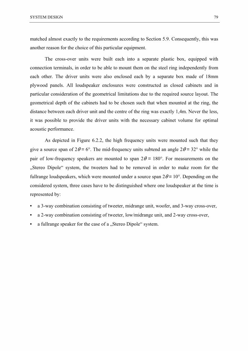
SYSTEM DESIGN 79
matched almost exactly to the requirements according to Section 5.9. Consequently, this was
another reason for the choice of this particular equipment.
The cross-over units were built each into a separate plastic box, equipped with
connection terminals, in order to be able to mount them on the steel ring independently from
each other. The driver units were also enclosed each by a separate box made of 18mm
plywood panels. All loudspeaker enclosures were constructed as closed cabinets and in
particular consideration of the geometrical limitations due to the required source layout. The
geometrical depth of the cabinets had to be chosen such that when mounted at the ring, the
distance between each driver unit and the centre of the ring was exactly 1,4m. Never the less,
it was possible to provide the driver units with the necessary cabinet volume for optimal
acoustic performance.
As depicted in Figure 6.2.2, the high frequency units were mounted such that they
give a source span of 2θ = 6°. The mid-frequency units subtend an angle 2θ = 32° while the
pair of low-frequency speakers are mounted to span 2θ = 180°. For measurements on the
„Stereo Dipole“ system, the tweeters had to be removed in order to make room for the
fullrange loudspeakers, which were mounted under a source span 2θ = 10°. Depending on the
considered system, three cases have to be distinguished where one loudspeaker at the time is
represented by:
• a 3-way combination consisting of tweeter, midrange unit, woofer, and 3-way cross-over,
• a 2-way combination consisting of tweeter, low/midrange unit, and 2-way cross-over,
• a fullrange speaker for the case of a „Stereo Dipole“ system.
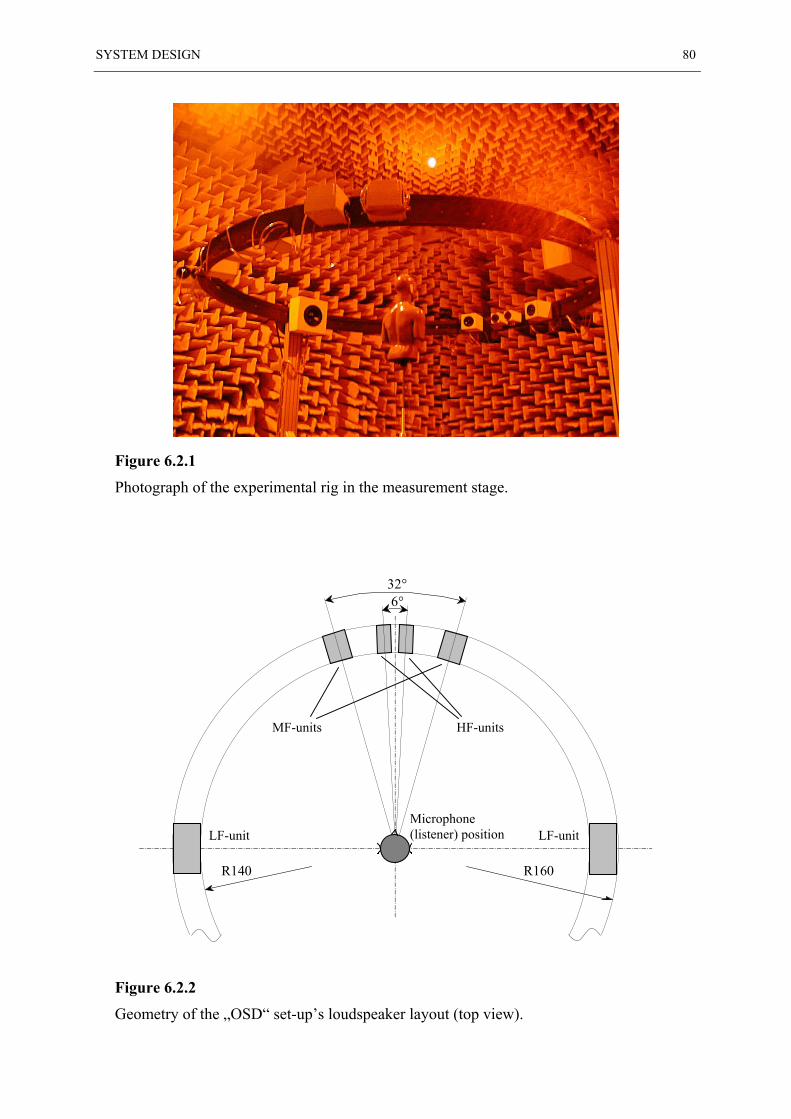
SYSTEM DESIGN 80
Figure
Photogr
Figure
Geomet
6.2.1
aph of the experimental rig in the measurement stage.
6.2.2
ry of the „OSD“ set-up’s loudspeaker layout (top view).
32°6°
R160R140
LF-unit LF-unit
MF-units HF-units
Microphone(listener) position
SYSTEM DESIGN 81
6.3 Measurements of the Plant Matrix
As discussed earlier, the task of binaural virtual acoustic imaging with loudspeakers requires
an appropriate inverse filtering for the crosstalk cancellation. Thus, the system's plant matrix
of the electro-acoustic paths C has to be measured. In consideration of section 5.10, there are
various options of obtaining the plant, which differ mainly depending on where the cross-
over network is inserted to the system. Therefore, measurements were made for the two
different „OSD“ systems (3-way and 2-way) and the „Stereo Dipole“ system as well as for
every single loudspeaker of the arrangements separately. This was made in order to provide
data about the appropriate plants for all of those different options. Some of them may be
subject of investigations in future experiments. For the present experiment, only the data for
"OSD" systems including the cross-over filter network were used to calculate the crosstalk
cancellation filters H. As shown in Figure 5.10.1, the plant C consists of a [2 × 2] matrix of
electro-acoustic transfer functions in this case. The response of the cross-over filters is
already included in the plant measurement. Consequently, the obtained inverse filter matrix
H automatically compensates for the cross-over network as well as for the interaction
between different pairs of driver units around the cut-off frequencies of the cross-over filters.
Measurements were made of four impulse responses that represent the Head-Related
Transfer Functions (HRTFs) in the time domain between the two loudspeakers and the two
ears of a KEMAR dummy head. The dummy head was positioned at the centre of the steel
ring such that the distance of the KEMAR’s centre to each speaker was 1,4m.
In order to obtain two different sets of HRTF measurements at once, two different
pinna styles were installed on the KEMAR. The left was the smaller model DB-061 and the
right was the larger model DB-065. Assuming the KEMAR had perfect medial symmetry,
including the pinnae, the resulting sets of HRTF measurements would be symmetric within
the limits of measurement accuracy. In other words, two complete sets of measurements can
be obtained by mirroring the two half sets on the median plane. This was also done with
respect to the HRTF measurements of the KEMAR accomplished by Gardner and Martin
[1994], since their set of HRTFs was applied later for the binaural synthesis of virtual
acoustic images. Thus, the option of trying both ear type’s HRTFs was left open and it had
not to be decided in the measurement stage of the project which set to use later on.
Generally, the measurements always include not only the HRTFs but also the
SYSTEM DESIGN 82
response of the measurement system itself, consisting of the loudspeakers, the microphones,
D/A and A/D converters, anti-alias filters, audio and microphone amplifiers, and inevitably
some room characteristics. Interference due to reflections can be avoided by ensuring that
they occur well after the head response time, which is several milliseconds. This is certainly
the case for room reflections but some reflections off certain obstacles of the experimental
set-up might falsify the measurements slightly. Therefore, additional measurements were
made of all loudspeakers and the two “OSD” systems. This system's free-field response may
be deconvolved from the HRTF data if necessary. The measurement method (to be discussed
in the following section) was exactly the same as for the HRTF measurements, except that
the KEMAR dummy head was replaced by a single microphone, in particular the one which
was mounted in KEMAR’s right ear.
6.4 Measurement Method
The impulse responses were obtained using a maximum length sequence (MLS) measurement
technique. This method which is based on a time-domain cross-correlation between input and
output signal and is implemented in the MLSSA1 computer package [Rife, 1994]. MLSSA is
based on a DSP card installed in a personal computer and the software is running either in
DOS or Windows environments. The main advantage of MLSSA over other measurement
methods such as FFT frequency analyser, is the high noise and distortion immunity due to
pre-averaging techniques and the capability to measure long impulse responses quickly [Rife
and Vanderkooy, 1989; Vanderkooy, 1994]. Interfering background noise in the
measurement is reduced by means of pre-averaging of the measurement system's output. This
is possible since background noise is usually equally distributed over the measurement time.
The averaging is made prior to the cross-correlation process, which is indicated by the term
"pre-averaging". By this means, the signal-to-noise ratio is increased by 3dB per
measurement doubling. Errors due to non-linearities (e.g., caused by the loudspeakers) result,
unlike background noise, in rather impulsive and non-uniformly spread irregularities in the
1 MLSSA (Maximum Length Sequence System Analyser) is a trademark of DRA laboratories.
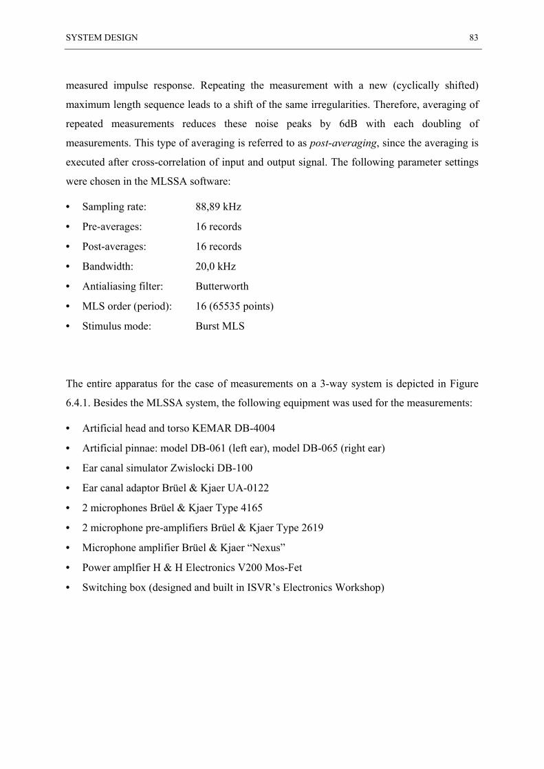
SYSTEM DESIGN 83
measured impulse response. Repeating the measurement with a new (cyclically shifted)
maximum length sequence leads to a shift of the same irregularities. Therefore, averaging of
repeated measurements reduces these noise peaks by 6dB with each doubling of
measurements. This type of averaging is referred to as post-averaging, since the averaging is
executed after cross-correlation of input and output signal. The following parameter settings
were chosen in the MLSSA software:
• Sampling rate: 88,89 kHz
• Pre-averages: 16 records
• Post-averages: 16 records
• Bandwidth: 20,0 kHz
• Antialiasing filter: Butterworth
• MLS order (period): 16 (65535 points)
• Stimulus mode: Burst MLS
The entire apparatus for the case of measurements on a 3-way system is depicted in Figure
6.4.1. Besides the MLSSA system, the following equipment was used for the measurements:
• Artificial head and torso KEMAR DB-4004
• Artificial pinnae: model DB-061 (left ear), model DB-065 (right ear)
• Ear canal simulator Zwislocki DB-100
• Ear canal adaptor Brüel & Kjaer UA-0122
• 2 microphones Brüel & Kjaer Type 4165
• 2 microphone pre-amplifiers Brüel & Kjaer Type 2619
• Microphone amplifier Brüel & Kjaer “Nexus”
• Power amplfier H & H Electronics V200 Mos-Fet
• Switching box (designed and built in ISVR’s Electronics Workshop)
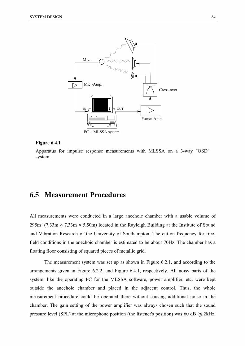
SYSTEM DESIGN 84
Figure 6.4.1
Apparatus for impulse response measurements with MLSSA on a 3-way "OSD"system.
6.5 Measurement Procedures
All measurements were conducted in a large anechoic chamber with a usable volume of
295m3 (7,33m × 7,33m × 5,50m) located in the Rayleigh Building at the Institute of Sound
and Vibration Research of the University of Southampton. The cut-on frequency for free-
field conditions in the anechoic chamber is estimated to be about 70Hz. The chamber has a
floating floor consisting of squared pieces of metallic grid.
The measurement system was set up as shown in Figure 6.2.1, and according to the
arrangements given in Figure 6.2.2, and Figure 6.4.1, respectively. All noisy parts of the
system, like the operating PC for the MLSSA software, power amplifier, etc. were kept
outside the anechoic chamber and placed in the adjacent control. Thus, the whole
measurement procedure could be operated there without causing additional noise in the
chamber. The gain setting of the power amplifier was always chosen such that the sound
pressure level (SPL) at the microphone position (the listener's position) was 60 dB @ 2kHz.
Power-Amp.
Cross-over
Mic.
PC + MLSSA system
OUTIN
Mic.-Amp.
SYSTEM DESIGN 85
This was controlled with a sound level meter since the same SPL was intended to use for the
later subjective experiments. Only for the direct measurements on the high frequency units,
the gain was reduced significantly in order to avoid damage due to the low-frequency content
in the MLS signal.
The position of the free-field microphone was calibrated by means of "trial-and-error"
impulse response measurements. Thereby, the time delays between two opposite loud-
speakers were compared and the microphone was moved around until both impulse responses
had the same delay (± 1 sample). This comparison was done between both corresponding
loudspeakers left and right and corresponding loudspeakers in front and behind the
microphone position. Therefore, the same set of loudspeakers (apart from the woofers) was
installed on both sides of the steel ring, in front and in the rear of the listener (microphone).
This can be recognised on the left of Figure 6.2.1. The correct height of the microphone was
controlled with a tape measure and two pieces of string which were spanned each between
two opposite facing holes in the steel ring.
For the HRTF measurements, the KEMAR dummy head was mounted in the middle
of the loudspeaker arrangement. The correct alignment of the KEMAR was achieved in a
similar manner. Because the KEMAR was equipped with two different pinna types, they
were removed and hence only the microphones in the two ear canals were used for the
alignment process to ensure symmetry. The point of origin in terms of "left-right" position
was reached when the time delays between left microphone and left woofer and between
right microphone and right woofer, respectively, were equal (± 1 sample). In the same way,
the impulse responses between the midrange units and the respective opposite ear were
compared to ensure the KEMAR wasn't rotated towards either side. The height and the
"front-back" position of the two ears (microphones) were again aligned with spanned strings.
SYSTEM DESIGN 86
6.6 Processing and Data Reduction
Each measurement yielded a 65535 points impulse response at a fS = 88,89 kHz sampling
frequency. Most of these data are irrelevant since the length of the stored responses is larger
than necessary to cover the duration of the response of interest. The 1,4m air travel between
the loudspeakers and the microphones corresponds to about 360 samples. After this initial
delay follows the system response, which persists typically only a few milliseconds in the
case of a head response (HRTF). Data after the system response are due to reflections off
objects in the anechoic chamber such as the steel ring and other reflecting obstacles of the
experimental rig.
In order to reduce the size of the data set without eliminating anything of potential
interest, the first 360 samples of each impulse response were discarded. The following
samples were truncated where the response became smallest just before the onset of the first
major reflection. This was after around 900 samples (~10 msec) but the exact number varies
for each conditions and units. The truncation of the impulse response data is known to
introduce ripples in the frequency domain, an effect referred to as the Gibbs phenomenon
[Oppenheim and Schafer, 1975]. Therefore, the retained data were multiplied with a half
Hanning window in order to smooth the response and alleviate the effect of ripples.
Before the impulse response was further processed for the implementation of
crosstalk-cancellation filters, the data were downsampled by the factor 2, i.e., every second
sample was left out. It should be noted that there was a slight discrepancy between the
sampling rate resulting from the downsampling, which is fS = 44,445 kHz and the usual
sampling frequency fS = 44,1 kHz. However, it was assumed that this error would not affect
the later subjective experiments significantly. In fact, considering the HRTF measurements,
this sampling rate difference corresponds to a negligible enlargement of the geometrical head
dimensions. In other words, the effect is the same as when the KEMAR was larger of the
factor 1,0078 when measuring with fS = 44,1 kHz. Seeing that the morphological dimensions
of KEMAR appear fairly small compared to a typical size European head, this might even be
a desirable effect than a drawback due to the awkward parameter options with MLSSA.
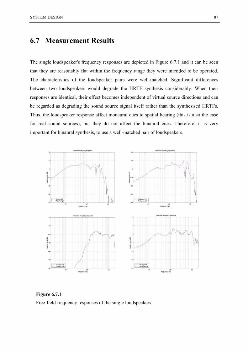
SYSTEM DESIGN 87
6.7 Measurement Results
The single loudspeaker's frequency responses are depicted in Figure 6.7.1 and it can be seen
that they are reasonably flat within the frequency range they were intended to be operated.
The characteristics of the loudspeaker pairs were well-matched. Significant differences
between two loudspeakers would degrade the HRTF synthesis considerably. When their
responses are identical, their effect becomes independent of virtual source directions and can
be regarded as degrading the sound source signal itself rather than the synthesised HRTFs.
Thus, the loudspeaker response affect monaural cues to spatial hearing (this is also the case
for real sound sources), but they do not affect the binaural cues. Therefore, it is very
important for binaural synthesis, to use a well-matched pair of loudspeakers.
Figure 6.7.1
Free-field frequency responses of the single loudspeakers.
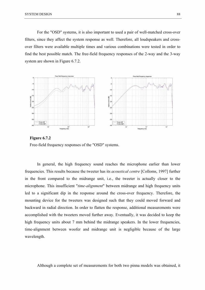
SYSTEM DESIGN 88
For the "OSD" systems, it is also important to used a pair of well-matched cross-over
filters, since they affect the system response as well. Therefore, all loudspeakers and cross-
over filters were available multiple times and various combinations were tested in order to
find the best possible match. The free-field frequency responses of the 2-way and the 3-way
system are shown in Figure 6.7.2.
Figure 6.7.2
Free-field frequency responses of the "OSD" systems.
In general, the high frequency sound reaches the microphone earlier than lower
frequencies. This results because the tweeter has its acoustical centre [Colloms, 1997] further
in the front compared to the midrange unit, i.e., the tweeter is actually closer to the
microphone. This insufficient "time-alignment" between midrange and high frequency units
led to a significant dip in the response around the cross-over frequency. Therefore, the
mounting device for the tweeters was designed such that they could moved forward and
backward in radial direction. In order to flatten the response, additional measurements were
accomplished with the tweeters moved further away. Eventually, it was decided to keep the
high frequency units about 7 mm behind the midrange speakers. In the lower frequencies,
time-alignment between woofer and midrange unit is negligible because of the large
wavelength.
Although a complete set of measurements for both two pinna models was obtained, it
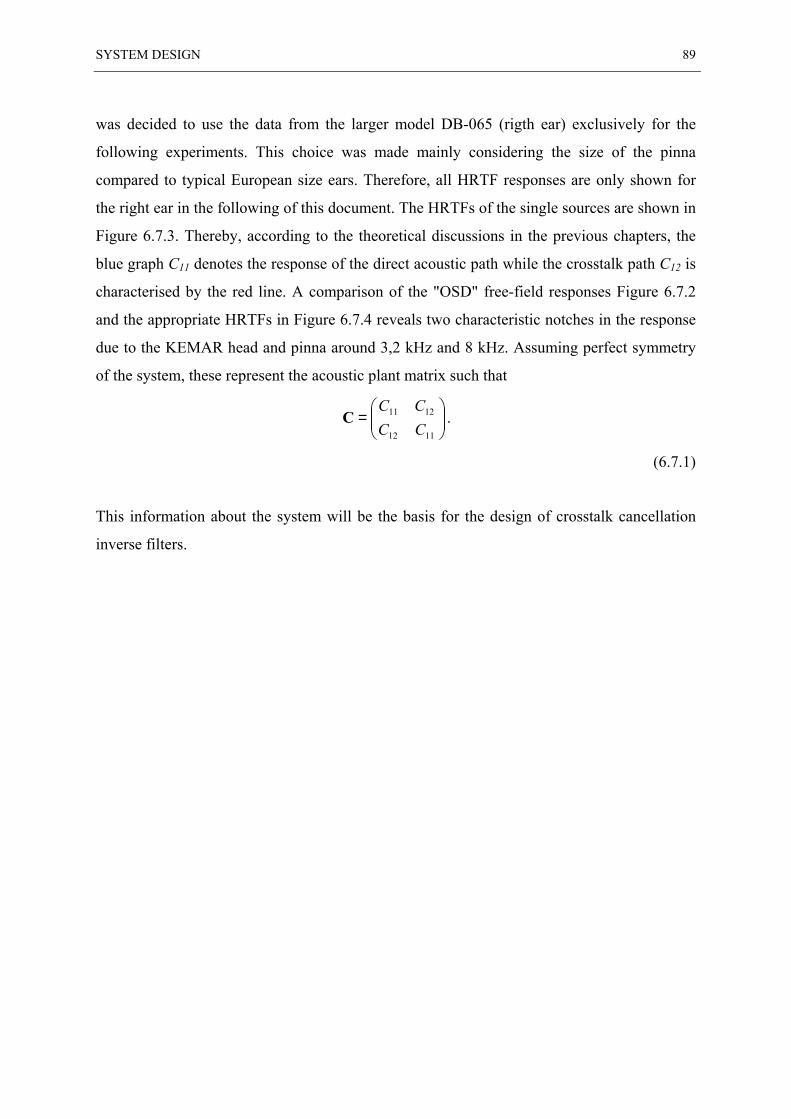
SYSTEM DESIGN 89
was decided to use the data from the larger model DB-065 (rigth ear) exclusively for the
following experiments. This choice was made mainly considering the size of the pinna
compared to typical European size ears. Therefore, all HRTF responses are only shown for
the right ear in the following of this document. The HRTFs of the single sources are shown in
Figure 6.7.3. Thereby, according to the theoretical discussions in the previous chapters, the
blue graph C11 denotes the response of the direct acoustic path while the crosstalk path C12 is
characterised by the red line. A comparison of the "OSD" free-field responses Figure 6.7.2
and the appropriate HRTFs in Figure 6.7.4 reveals two characteristic notches in the response
due to the KEMAR head and pinna around 3,2 kHz and 8 kHz. Assuming perfect symmetry
of the system, these represent the acoustic plant matrix such that
=
1112
1211
CCCC
C .
(6.7.1)
This information about the system will be the basis for the design of crosstalk cancellation
inverse filters.
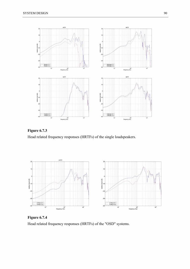
SYSTEM DESIGN 90
Figure 6.7.3
Head related frequency responses (HRTFs) of the single loudspeakers.
Figure 6.7.4
Head related frequency responses (HRTFs) of the "OSD" systems.
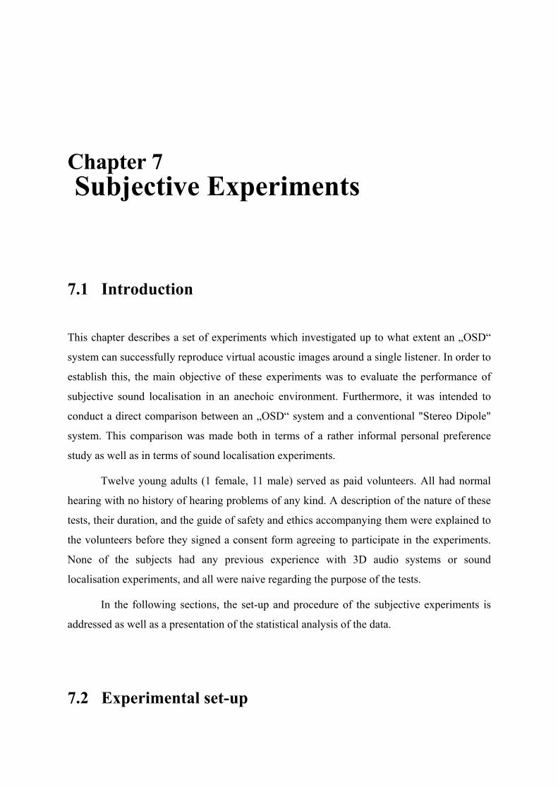
Chapter 7 Subjective Experiments
7.1 Introduction
This chapter describes a set of experiments which investigated up to what extent an „OSD“
system can successfully reproduce virtual acoustic images around a single listener. In order to
establish this, the main objective of these experiments was to evaluate the performance of
subjective sound localisation in an anechoic environment. Furthermore, it was intended to
conduct a direct comparison between an „OSD“ system and a conventional "Stereo Dipole"
system. This comparison was made both in terms of a rather informal personal preference
study as well as in terms of sound localisation experiments.
Twelve young adults (1 female, 11 male) served as paid volunteers. All had normal
hearing with no history of hearing problems of any kind. A description of the nature of these
tests, their duration, and the guide of safety and ethics accompanying them were explained to
the volunteers before they signed a consent form agreeing to participate in the experiments.
None of the subjects had any previous experience with 3D audio systems or sound
localisation experiments, and all were naive regarding the purpose of the tests.
In the following sections, the set-up and procedure of the subjective experiments is
addressed as well as a presentation of the statistical analysis of the data.
7.2 Experimental set-up
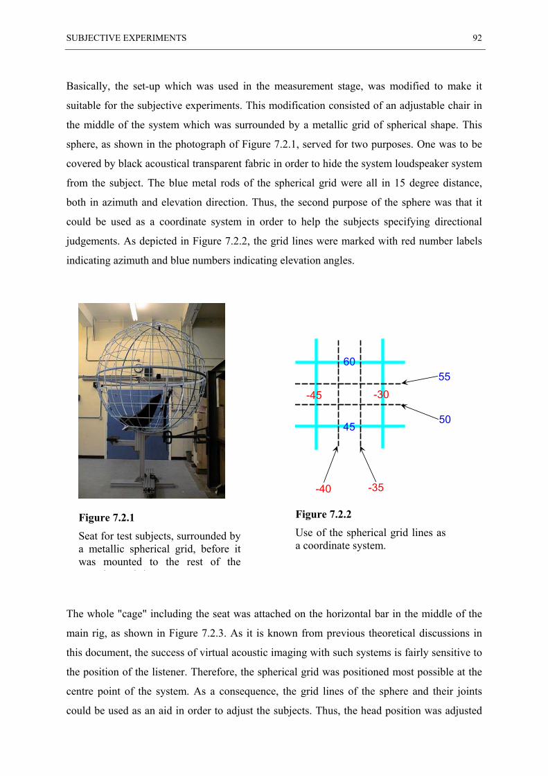
SUBJECTIVE EXPERIMENTS 92
Basically, the set-up which was used in the measurement stage, was modified to make it
suitable for the subjective experiments. This modification consisted of an adjustable chair in
the middle of the system which was surrounded by a metallic grid of spherical shape. This
sphere, as shown in the photograph of Figure 7.2.1, served for two purposes. One was to be
covered by black acoustical transparent fabric in order to hide the system loudspeaker system
from the subject. The blue metal rods of the spherical grid were all in 15 degree distance,
both in azimuth and elevation direction. Thus, the second purpose of the sphere was that it
could be used as a coordinate system in order to help the subjects specifying directional
judgements. As depicted in Figure 7.2.2, the grid lines were marked with red number labels
indicating azimuth and blue numbers indicating elevation angles.
T as attached on the horizontal bar in the middle of the
m
th
th
ce
co
-45 -30
45
60
-40 -35
50
55
Figure 7.2.2
Use of the spherical grid lines asa coordinate system.
he whole "cage" including the seat w
Figure 7.2.1
Seat for test subjects, surrounded bya metallic spherical grid, before itwas mounted to the rest of the
i l i
ain rig, as shown in Figure 7.2.3. As it is known from previous theoretical discussions in
is document, the success of virtual acoustic imaging with such systems is fairly sensitive to
e position of the listener. Therefore, the spherical grid was positioned most possible at the
ntre point of the system. As a consequence, the grid lines of the sphere and their joints
uld be used as an aid in order to adjust the subjects. Thus, the head position was adjusted
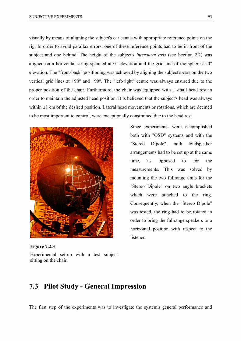
SUBJECTIVE EXPERIMENTS 93
visually by means of aligning the subject's ear canals with appropriate reference points on the
rig. In order to avoid parallax errors, one of these reference points had to be in front of the
subject and one behind. The height of the subject's interaural axis (see Section 2.2) was
aligned on a horizontal string spanned at 0° elevation and the grid line of the sphere at 0°
elevation. The "front-back" positioning was achieved by aligning the subject's ears on the two
vertical grid lines at +90° and −90°. The "left-right" centre was always ensured due to the
proper position of the chair. Furthermore, the chair was equipped with a small head rest in
order to maintain the adjusted head position. It is believed that the subject's head was always
within ±1 cm of the desired position. Lateral head movements or rotations, which are deemed
to be most important to control, were exceptionally constrained due to the head rest.
Since experiments were accomplished
both with "OSD" systems and with the
"Stereo Dipole", both loudspeaker
arrangements had to be set up at the same
time, as opposed to for the
measurements. This was solved by
mounting the two fullrange units for the
"Stereo Dipole" on two angle brackets
which were attached to the ring.
Consequently, when the "Stereo Dipole"
was tested, the ring had to be rotated in
order to bring the fullrange speakers to a
horizontal position with respect to the
listener.
7.3 Pilot Study - General Impression
The first step of the experiments was to investigate the system's general performance and
Figure 7.2.3
Experimental set-up with a test subjectsitting on the chair.
SUBJECTIVE EXPERIMENTS 94
whether the system is able to create virtual acoustic images at all. For these purposes,
crosstalk cancellation filters were implemented based on the previously measured system
plants. All filters were calcualted off-line in MATLAB1. The algorithm for the system
inversion was implemented in the frequency domain, based on the method of fast
deconvolution using regularisation [Kirkeby et al., 1996a], as it was discussed previously in
Chapter 4. For all investigated system configurations, the inversion process was regularised
to ensure about 20dB dynamic range loss, according to the considerations in Chapter 5.
Further processing which was included later for the binaural synthesis of virtual sources,
would lead to additional dynamic range loss (or sometimes gain). The caculated inverse
filters were implemented in the HURON2 digital audio convolution workstation, using 8638-
point FIR filters. The HURON workstation utilises low-latency convolution algorithms to
enable the convolution of signals and impulse responses in real-time.
For initial trials, binaural recordings of sounds in the nature3 on Compact Disc were
used as source signals. Most of these recordings were reported to be made with the "Aachen
Head", an artficial head microphone from Head Acoustics, Germany. The CD-signal was fed
into the input of the Huron where the signal was processed with the appropriate inverse
filters, depending on the system under investigation. A rather informal study was undertaken
by comparing the general impression of the three evaluated systems.
The most remarkable difference was the far wider lateral range of the sound stage
with the use of an "OSD" system as opposed to the "Stereo Dipole" configuration. In fact, all
participating listeners reacted amazed and where overwhelmed by the clarity of the sound
images and how differentiated one could perceive particular details in the recordings. This
was also true for a 2-way system but clearly the 3-way "OSD" system left the best
impression.
One reason for this unisonous preference probably were the additional woofer speakers. Due
to the better low-frequency reproduction, the system itself just sounded more impressing.
Hence, there was no evidence yet that the performance in terms of convincing virtual
acoustic imaging and sound localisation accuracy was superior compared to the other
systems. Therefore, more sophisticated and extensive listening tests were undertaken in order
1 The MathWorks, Inc.2 Lake DSP Pty Ltd., Ultimo, Australia.3 Published by the Japan Audio Society.
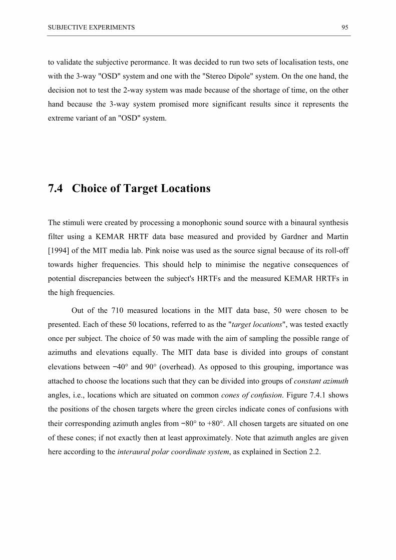
SUBJECTIVE EXPERIMENTS 95
to validate the subjective perormance. It was decided to run two sets of localisation tests, one
with the 3-way "OSD" system and one with the "Stereo Dipole" system. On the one hand, the
decision not to test the 2-way system was made because of the shortage of time, on the other
hand because the 3-way system promised more significant results since it represents the
extreme variant of an "OSD" system.
7.4 Choice of Target Locations
The stimuli were created by processing a monophonic sound source with a binaural synthesis
filter using a KEMAR HRTF data base measured and provided by Gardner and Martin
[1994] of the MIT media lab. Pink noise was used as the source signal because of its roll-off
towards higher frequencies. This should help to minimise the negative consequences of
potential discrepancies between the subject's HRTFs and the measured KEMAR HRTFs in
the high frequencies.
Out of the 710 measured locations in the MIT data base, 50 were chosen to be
presented. Each of these 50 locations, referred to as the "target locations", was tested exactly
once per subject. The choice of 50 was made with the aim of sampling the possible range of
azimuths and elevations equally. The MIT data base is divided into groups of constant
elevations between −40° and 90° (overhead). As opposed to this grouping, importance was
attached to choose the locations such that they can be divided into groups of constant azimuth
angles, i.e., locations which are situated on common cones of confusion. Figure 7.4.1 shows
the positions of the chosen targets where the green circles indicate cones of confusions with
their corresponding azimuth angles from −80° to +80°. All chosen targets are situated on one
of these cones; if not exactly then at least approximately. Note that azimuth angles are given
here according to the interaural polar coordinate system, as explained in Section 2.2.
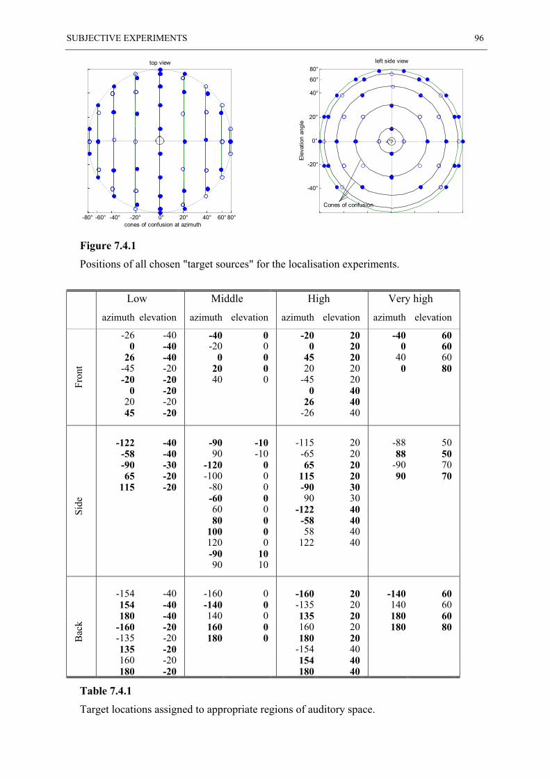
SUBJECTIVE EXPERIMENTS 96
80°left side view
top viewFigure 7.4.1
Positions of all chosen "target sources" for the localisation experiments.
Low Middle High Very high
azimuth elevation azimuth elevation azimuth elevation azimuth elevation
-26 -40 -40 0 -20 20 -40 600 -40 -20 0 0 20 0 60
26 -40 0 0 45 20 40 60-45 -20 20 0 20 20 0 80-20 -20 40 0 -45 20
0 -20 0 4020 -20 26 40
Fron
t
45 -20 -26 40
-122 -40 -90 -10 -115 20 -88 50-58 -40 90 -10 -65 20 88 50-90 -30 -120 0 65 20 -90 7065 -20 -100 0 115 20 90 70
115 -20 -80 0 -90 30-60 0 90 3060 0 -122 4080 0 -58 40
100 0 58 40120 0 122 40-90 10
Side
90 10
-154 -40 -160 0 -160 20 -140 60154 -40 -140 0 -135 20 140 60180 -40 140 0 135 20 180 60
-160 -20 160 0 160 20 180 80-135 -20 180 0 180 20135 -20 -154 40160 -20 154 40
Bac
k
180 -20 180 40
Table 7.4.1
Target locations assigned to appropriate regions of auditory space.
-80° -40° -20° 0° 20° 40° 80°-60°cones of confusion at azimuth
60°
-40°
-20°
0°
20°
40°
Elev
atio
n an
gle
60°
Cones of confusion
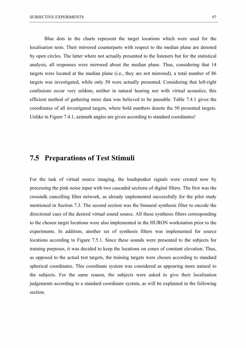
SUBJECTIVE EXPERIMENTS 97
Blue dots in the charts represent the target locations which were used for the
localisation tests. Their mirrored counterparts with respect to the median plane are denoted
by open circles. The latter where not actually presented to the listeners but for the statistical
analysis, all responses were mirrored about the median plane. Thus, considering that 14
targets were located at the median plane (i.e., they are not mirrored), a total number of 86
targets was investigated, while only 50 were actually presented. Considering that left-right
confusions occur very seldom, neither in natural hearing nor with virtual acoustics, this
efficient method of gathering more data was believed to be passable. Table 7.4.1 gives the
coordinates of all investigated targets, where bold numbers denote the 50 presented targets.
Unlike in Figure 7.4.1, azimuth angles are given according to standard coordinates!
7.5 Preparations of Test Stimuli
For the task of virtual source imaging, the loudspeaker signals were created now by
processing the pink noise input with two cascaded sections of digital filters. The first was the
crosstalk cancelling filter network, as already implemented successfully for the pilot study
mentioned in Section 7.3. The second section was the binaural synthesis filter to encode the
directional cues of the desired virtual sound source. All these synthesis filters corresponding
to the chosen target locations were also implemented in the HURON workstation prior to the
experiments. In addition, another set of synthesis filters was implemented for source
locations according to Figure 7.5.1. Since these sounds were presented to the subjects for
training purposes, it was decided to keep the locations on cones of constant elevation. Thus,
as opposed to the actual test targets, the training targets were chosen according to standard
spherical coordinates. This coordinate system was considered as appearing more natural to
the subjects. For the same reason, the subjects were asked to give their localisation
judgements according to a standard coordinate system, as will be explained in the following
section.
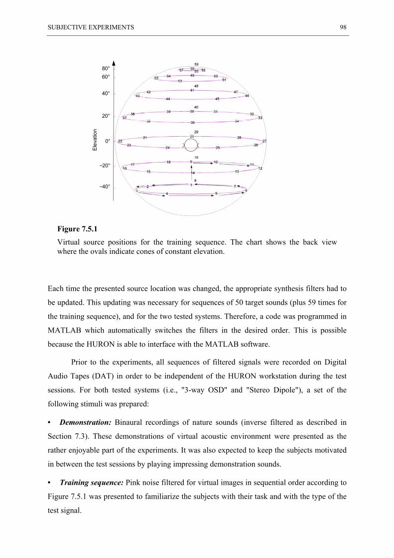
SUBJECTIVE EXPERIMENTS 98
Figure 7.5.1
Virtual source positions for the training sequence. The chart shows the back viewwhere the ovals indicate cones of constant elevation.
Each time the presented source location was changed, the appropriate synthesis filters had to
be updated. This updating was necessary for sequences of 50 target sounds (plus 59 times for
the training sequence), and for the two tested systems. Therefore, a code was programmed in
MATLAB which automatically switches the filters in the desired order. This is possible
because the HURON is able to interface with the MATLAB software.
Prior to the experiments, all sequences of filtered signals were recorded on Digital
Audio Tapes (DAT) in order to be independent of the HURON workstation during the test
sessions. For both tested systems (i.e., "3-way OSD" and "Stereo Dipole"), a set of the
following stimuli was prepared:
• Demonstration: Binaural recordings of nature sounds (inverse filtered as described in
Section 7.3). These demonstrations of virtual acoustic environment were presented as the
rather enjoyable part of the experiments. It was also expected to keep the subjects motivated
in between the test sessions by playing impressing demonstration sounds.
• Training sequence: Pink noise filtered for virtual images in sequential order according to
Figure 7.5.1 was presented to familiarize the subjects with their task and with the type of the
test signal.
−40°
80°60°
40°
20°
0°
−20°
Elev
atio
n
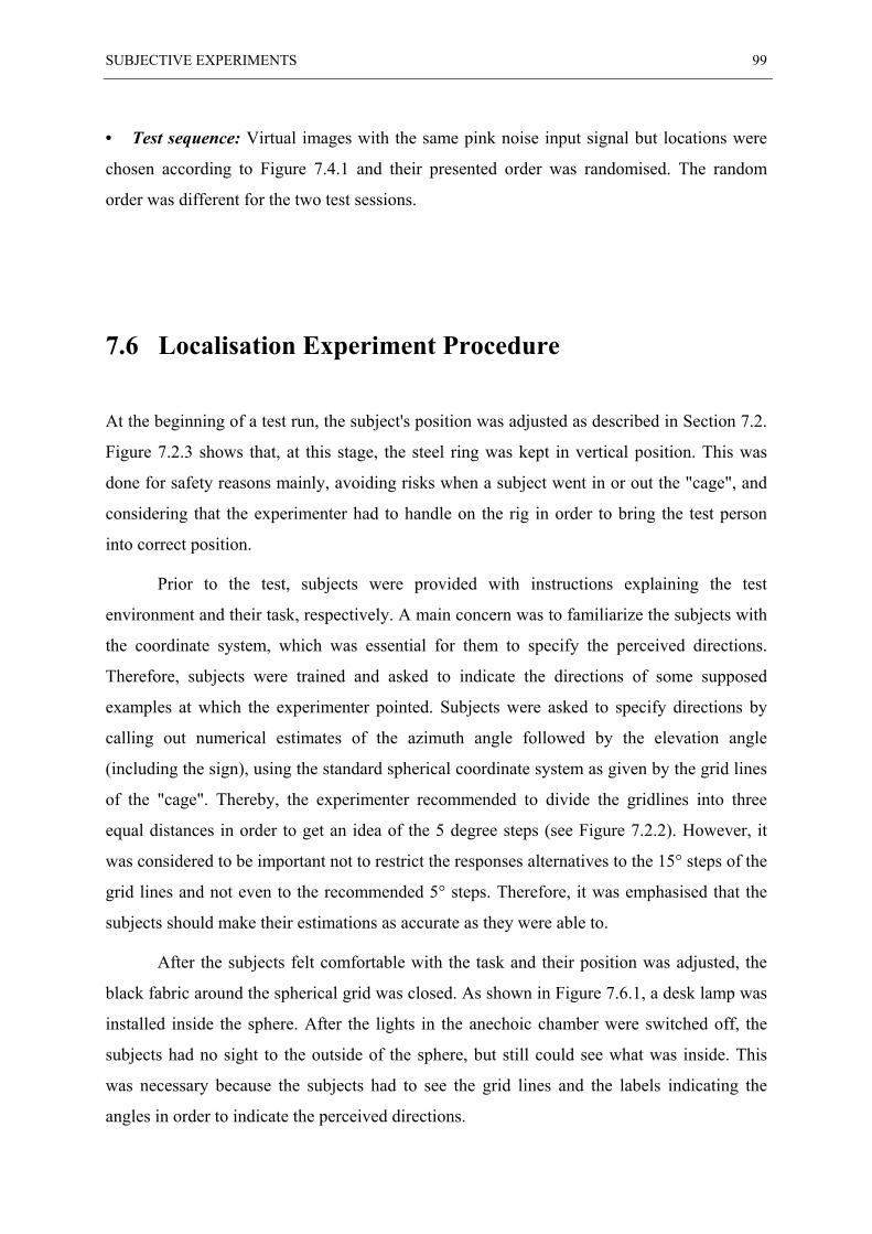
SUBJECTIVE EXPERIMENTS 99
• Test sequence: Virtual images with the same pink noise input signal but locations were
chosen according to Figure 7.4.1 and their presented order was randomised. The random
order was different for the two test sessions.
7.6 Localisation Experiment Procedure
At the beginning of a test run, the subject's position was adjusted as described in Section 7.2.
Figure 7.2.3 shows that, at this stage, the steel ring was kept in vertical position. This was
done for safety reasons mainly, avoiding risks when a subject went in or out the "cage", and
considering that the experimenter had to handle on the rig in order to bring the test person
into correct position.
Prior to the test, subjects were provided with instructions explaining the test
environment and their task, respectively. A main concern was to familiarize the subjects with
the coordinate system, which was essential for them to specify the perceived directions.
Therefore, subjects were trained and asked to indicate the directions of some supposed
examples at which the experimenter pointed. Subjects were asked to specify directions by
calling out numerical estimates of the azimuth angle followed by the elevation angle
(including the sign), using the standard spherical coordinate system as given by the grid lines
of the "cage". Thereby, the experimenter recommended to divide the gridlines into three
equal distances in order to get an idea of the 5 degree steps (see Figure 7.2.2). However, it
was considered to be important not to restrict the responses alternatives to the 15° steps of the
grid lines and not even to the recommended 5° steps. Therefore, it was emphasised that the
subjects should make their estimations as accurate as they were able to.
After the subjects felt comfortable with the task and their position was adjusted, the
black fabric around the spherical grid was closed. As shown in Figure 7.6.1, a desk lamp was
installed inside the sphere. After the lights in the anechoic chamber were switched off, the
subjects had no sight to the outside of the sphere, but still could see what was inside. This
was necessary because the subjects had to see the grid lines and the labels indicating the
angles in order to indicate the perceived directions.
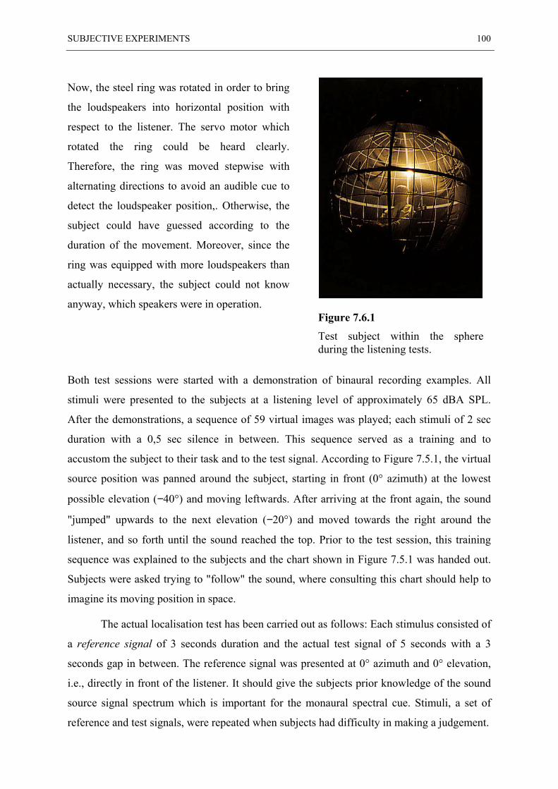
SUBJECTIVE EXPERIMENTS 100
Now, the steel ring was rotated in order to bring
the loudspeakers into horizontal position with
respect to the listener. The servo motor which
rotated the ring could be heard clearly.
Therefore, the ring was moved stepwise with
alternating directions to avoid an audible cue to
detect the loudspeaker position,. Otherwise, the
subject could have guessed according to the
duration of the movement. Moreover, since the
ring was equipped with more loudspeakers than
actually necessary, the subject could not know
anyway, which speakers were in operation.
Both test sessions were started with a demonstration of binaural recording examples. All
stimuli were presented to the subjects at a listening level of approximately 65 dBA SPL.
After the demonstrations, a sequence of 59 virtual images was played; each stimuli of 2 sec
duration with a 0,5 sec silence in between. This sequence served as a training and to
accustom the subject to their task and to the test signal. According to Figure 7.5.1, the virtual
source position was panned around the subject, starting in front (0° azimuth) at the lowest
possible elevation (−40°) and moving leftwards. After arriving at the front again, the sound
"jumped" upwards to the next elevation (−20°) and moved towards the right around the
listener, and so forth until the sound reached the top. Prior to the test session, this training
sequence was explained to the subjects and the chart shown in Figure 7.5.1 was handed out.
Subjects were asked trying to "follow" the sound, where consulting this chart should help to
imagine its moving position in space.
The actual localisation test has been carried out as follows: Each stimulus consisted of
a reference signal of 3 seconds duration and the actual test signal of 5 seconds with a 3
seconds gap in between. The reference signal was presented at 0° azimuth and 0° elevation,
i.e., directly in front of the listener. It should give the subjects prior knowledge of the sound
source signal spectrum which is important for the monaural spectral cue. Stimuli, a set of
reference and test signals, were repeated when subjects had difficulty in making a judgement.
Figure 7.6.1
Test subject within the sphereduring the listening tests.
SUBJECTIVE EXPERIMENTS 101
Subjects were asked to lean their head against the head rest in order to stay in position. They
were instructed to look always straight ahead and not to move the head (nor the body) while
any sounds were presented. Only after each set of reference and test sound had stopped,
subjects were allowed to move in order to look at the perceived direction and to work out the
appropriate coordinates. The experimenter, who was always present in a corner of the
anechoic chamber in order to operate the experiments, verified head position and stability.
The subject's responses were entered on a data sheet immediately after termination of
the stimuli. Thereby, no feedback was given to the subjects. When a sound was heard as
coming from more than one direction clearly or ambiguous among multiple directions,
subjects were asked to answer all apparent directions, as far as possible. Short breaks with
refreshments were given between the sessions. Subjects, who were all paid, were informed
that an additional award will be paid as a bonus for those who achieved a high score. Even
though it was just a matter of a small amount of money, this little psychological trick was
expected to help motivating the subjects.
7.7 Statistical analysis
Before analysing and discussing the results of the experiments, three principle types of errors
should be addressed the localisation performance is subject to. These are as follows:
• Systematic errors between the mean judged location and the target location that have the
form of a response bias. In free-field listening, these "localisation errors"1 are smallest in
azimuth judgements for frontal horizontal targets, and largest in elevation judgements for
rear medial targets. In the present experiment, additional errors over free-field conditions
are expected due to the systematic variation between the synthesis HRTFs and the listener
HRTFs. Furthermore, linear distortions in transmitting the binaural signals to the ears
might contribute errors.
• Usually, responses vary around the mean. Blauert [1997] defines the "localisation blur"
1 Term according to Blauert [1997].
SUBJECTIVE EXPERIMENTS 102
to be the amount of displacement of the target that is recognised by 50% of the listeners
as a change in judged location-in other words, the just noticeable difference. Rather than
using the strictly defined term "localisation blur", these errors will be called "response
variation" in this document.
• Front-back and up-down reversals (also called confusions): Errors are attributed to this
type, when the target location is confused with the mirror symmetric location obtained by
reflecting the target with respect to the frontal plane (for front-back reversals) or the
horizontal plane (for up-down reversals). Compared to front-back reversals, which are
very common, up-down reversals are less common and difficult to distinguish from other
types of errors.
Analysing the results of this sort of localisation experiments is complicated because the
stimuli and responses are represented by points in a three-dimensional space. In the present
case, points on the surface of a sphere are considered since the distance was constant. For
spherically organised data, the usual statistics (mean and variance) are either inappropriate or
potentially misleading. For example, using standard spherical coordinates, an azimuth error
of 30° for a source on the horizontal plane is much larger in an absolute distance sense than a
30° azimuth error for a point at 60° elevation. Therefore, azimuth judgements were analysed
based on a interaural spherical coordinate system. In other words, not the azimuth angles as
defined by a standard spherical coordinate system were treated, but the corresponding cones
of confusion of target and answer directions were compared. This means is advantageous
since the interaural differences (IID and ITD) are clearly represented between different cones
of confusion. In the same way as the cones of confusion represent the lateral displacement,
cones of constant elevation (as defined in Section 2.2 by a vertical polar coordinate system)1
give a sense of height. Hence, the performance in terms of elevation localisation was
investigated by comparing the elevation angles as they were reported by the subjects.
As a matter of fact, this kind of data analysis is only suitable to evaluate azimuth
localisation and elevation localisation, respectively. For example, it is impossible to detect
1 Note: For the definitions in Section 2.2, the terms "vertical polar" and "interaural polar" coordinate system,
SUBJECTIVE EXPERIMENTS 103
front-back reversals by this means. General statements about the localisation performance in
a three-dimensional sense are not possible either. Therefore, following Wightman and Kistler
[1989b], the following additional statistics will be used in order to characterise the results:
• Average angular error: -is defined as the mean unsigned angle, measured on a great
circle between each judgement vector and the corresponding vector from the origin to the
target position.
• Front-back reversals: If the angle between the target and the judgement is made smaller
by reflecting the judgement about the frontal plane, then the judgement was entered in
reflected form, and a counter for the number of front-back reversals was increased by
one. In other words, the reversals were counted and resolved before further analysis.
Front-to-back (F→B) reversals and back-to-front (B→F) reversals were classified
separately. The algorithm for resolving the reversals treats each judgement identically,
regardless of target azimuth. Hence, it undoubtedly produces a slight overestimate of
confusion rate and an underestimate of error angles for target positions near ±90°.
• Correlations: -between target and judgement azimuth and between target elevation and
judgement elevation angles.
Unlike Wenzel et al. [1993], no attempt was made to detect or correct up-down reversals,
because (considering own experience) it is believed most elevation judgements that would be
classified as up-down reversals are actually the result of localisation errors or localisation
blur.
• t-test: In practice of statistics, the "t-test" is usually applied in order to test whether the
means of two data series X and Y are significantly different or whether the difference is a
coincidence. According to Bronstein and Semendjajew [1996], the t-value is obtained by
( )( ) ( )( )( )
21
2121
22
21
2
11 nnnnnn
ynxn
yxt+
−+
∆−+∆−
−= ,
(7.7.1)
with x and y denoting the mean values, n1 and n2 are the numbers of data points, and ∆x and
∆y are the empirical variances of the data sets X and Y, respectively. With m = n1 + n2 −1 and
a chosen α-confidence interval, the critical t-value tα,m can be found according to a so-called
respectively, were used in stead of "standard spherical" and "interaural spherical" coordiante system.

SUBJECTIVE EXPERIMENTS 104
t-distribution. The means of the two data series are said to be significantly different, if
mtt ,α> .
(7.7.2)
This statement is subject to an error probability of α. For example, for α = 0,05 (as it was
chosen for our tests) and if the test series consist of 100 trials, the obtained result might be
wrong five times out of the 100.
Chapter 8 Results and Discussion
8.1 Introduction
In this chapter, results from the subjective experiments are summarized. As outlined in
Section 7.7, results have been analysed with respect to various aspects of sound localisation.
In principle, a comparison of the 3-way "OSD" system results and the "Stereo Dipole" system
results is shown, as far as possible. In order to detect individual differences, results have been
generally analysed for each subject separately, and overall mean values were calculated out
of them.
In the following, results in terms of azimuth and elevation localisation are summarised as
well as precision statistics such as correlation between judgement and target directions or
average angular errors. Individual response variations emerge most clearly in the percentage
of front-back reversals. A concluding discussion and proposals for potential future work is
given in a closing section.
8.2 Azimuth Localisation
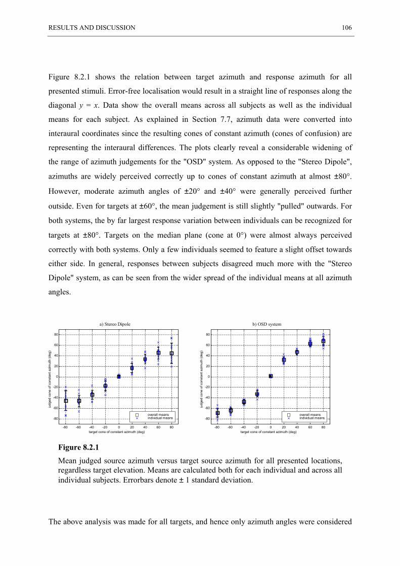
RESULTS AND DISCUSSION 106
Figure 8.2.1 shows the relation between target azimuth and response azimuth for all
presented stimuli. Error-free localisation would result in a straight line of responses along the
diagonal y = x. Data show the overall means across all subjects as well as the individual
means for each subject. As explained in Section 7.7, azimuth data were converted into
interaural coordinates since the resulting cones of constant azimuth (cones of confusion) are
representing the interaural differences. The plots clearly reveal a considerable widening of
the range of azimuth judgements for the "OSD" system. As opposed to the "Stereo Dipole",
azimuths are widely perceived correctly up to cones of constant azimuth at almost ±80°.
However, moderate azimuth angles of ±20° and ±40° were generally perceived further
outside. Even for targets at ±60°, the mean judgement is still slightly "pulled" outwards. For
both systems, the by far largest response variation between individuals can be recognized for
targets at ±80°. Targets on the median plane (cone at 0°) were almost always perceived
correctly with both systems. Only a few individuals seemed to feature a slight offset towards
either side. In general, responses between subjects disagreed much more with the "Stereo
Dipole" system, as can be seen from the wider spread of the individual means at all azimuth
angles.
80
a) Stereo Dipole
40
60
80
(deg
)
b) OSD system
40
60
(deg
)
Figure 8.2.1
Mean judged source azimuth versus target source azimuth for all presented locations,regardless target elevation. Means are calculated both for each individual and across allindividual subjects. Errorbars denote ± 1 standard deviation.
The above analysis was made for all targets, and hence only azimuth angles were considered
-80 -60 -40 -20 0 20 40 60 80
-80
-60
-40
-20
0
20
target cone of constant azimuth (deg)
judg
ed c
one
of c
onst
ant a
zimut
h
overall meansindividual means
-80 -60 -40 -20 0 20 40 60 80
-80
-60
-40
-20
0
20
target cone of constant azimuth (deg)
judg
ed c
one
of c
onst
ant a
zim
uth
overall meansindividual means
RESULTS AND DISCUSSION 107
regardless the elevation. Unlike this, Figure 8.2.2 and Figure 8.2.3 show results of the same
kind of investigations but analysed separately at four different groups of target elevation. For
the sake of clearness, individual means are omitted in these graphs but the standard deviation
bars give information about the interindividual response variations. The elevation range was
divided in accordance with Table 7.4.1 into the following groups:
• Low: −40° ≤ δ ≤ −20°
• Middle: −10° ≤ δ ≤ +10°
• High: +20° ≤ δ ≤ +40°
• Very high: +50° ≤ δ ≤ +80°
Generally, results from these charts look fairly similar compared to the overall results given
in Figure 8.2.1. The wider azimuth range with the "OSD" system is obtained at all elevations
as well as the slightly exaggerated judgements for moderate azimuth targets. Biased azimuth
estimations around the median plane, as mentioned above, seem to occur mainly for very
high elevated targets. Larger interindividual differences with the "Stereo Dipole", as seen
above, emerge here also at all target elevations.
Concluding, it can be stated that with both investigated systems the azimuth
localisation performance is generally independent of target elevations. In agreement with the
results of the pilot study, it is shown that with the "OSD" system azimuth angles are
perceived further outwards. Furthermore, the performance of azimuth judgements with
"OSD" is improved not only in terms of the correctly perceived range but also in terms of
more reliable estimations, as can be seen from the smaller response variation
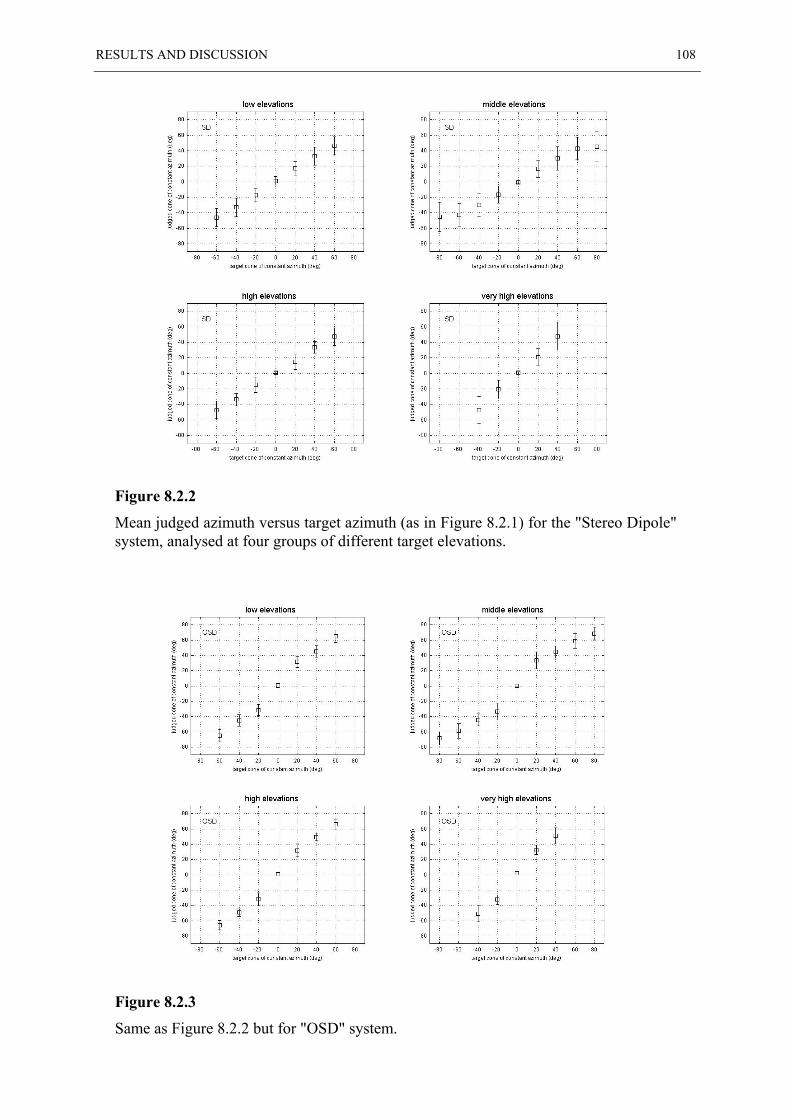
RESULTS AND DISCUSSION 108
Figure 8.2.2
Mean judged azimuth versus target azimuth (as in Figure 8.2.1) for the "Stereo Dipole"system, analysed at four groups of different target elevations.
Figure 8.2.3
Same as Figure 8.2.2 but for "OSD" system.
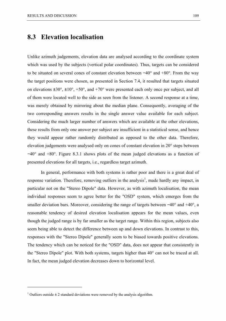
RESULTS AND DISCUSSION 109
8.3 Elevation localisation
Unlike azimuth judgements, elevation data are analysed according to the coordinate system
which was used by the subjects (vertical polar coordinates). Thus, targets can be considered
to be situated on several cones of constant elevation between −40° and +80°. From the way
the target positions were chosen, as presented in Section 7.4, it resulted that targets situated
on elevations ±30°, ±10°, +50°, and +70° were presented each only once per subject, and all
of them were located well to the side as seen from the listener. A second response at a time,
was merely obtained by mirroring about the median plane. Consequently, averaging of the
two corresponding answers results in the single answer value available for each subject.
Considering the much larger number of answers which are available at the other elevations,
these results from only one answer per subject are insufficient in a statistical sense, and hence
they would appear rather randomly distributed as opposed to the other data. Therefore,
elevation judgements were analysed only on cones of constant elevation in 20° steps between
−40° and +80°. Figure 8.3.1 shows plots of the mean judged elevations as a function of
presented elevations for all targets, i.e., regardless target azimuth.
In general, performance with both systems is rather poor and there is a great deal of
response variation. Therefore, removing outliers in the analysis1, made hardly any impact, in
particular not on the "Stereo Dipole" data. However, as with azimuth localisation, the mean
individual responses seem to agree better for the "OSD" system, which emerges from the
smaller deviation bars. Moreover, considering the range of targets between −40° and +40°, a
reasonable tendency of desired elevation localisation appears for the mean values, even
though the judged range is by far smaller as the target range. Within this region, subjects also
seem being able to detect the difference between up and down elevations. In contrast to this,
responses with the "Stereo Dipole" generally seem to be biased towards positive elevations.
The tendency which can be noticed for the "OSD" data, does not appear that consistently in
the "Stereo Dipole" plot. With both systems, targets higher than 40° can not be traced at all.
In fact, the mean judged elevation decreases down to horizontal level.
1 Outliers outside ± 2 standard deviations were removed by the analysis algorithm.
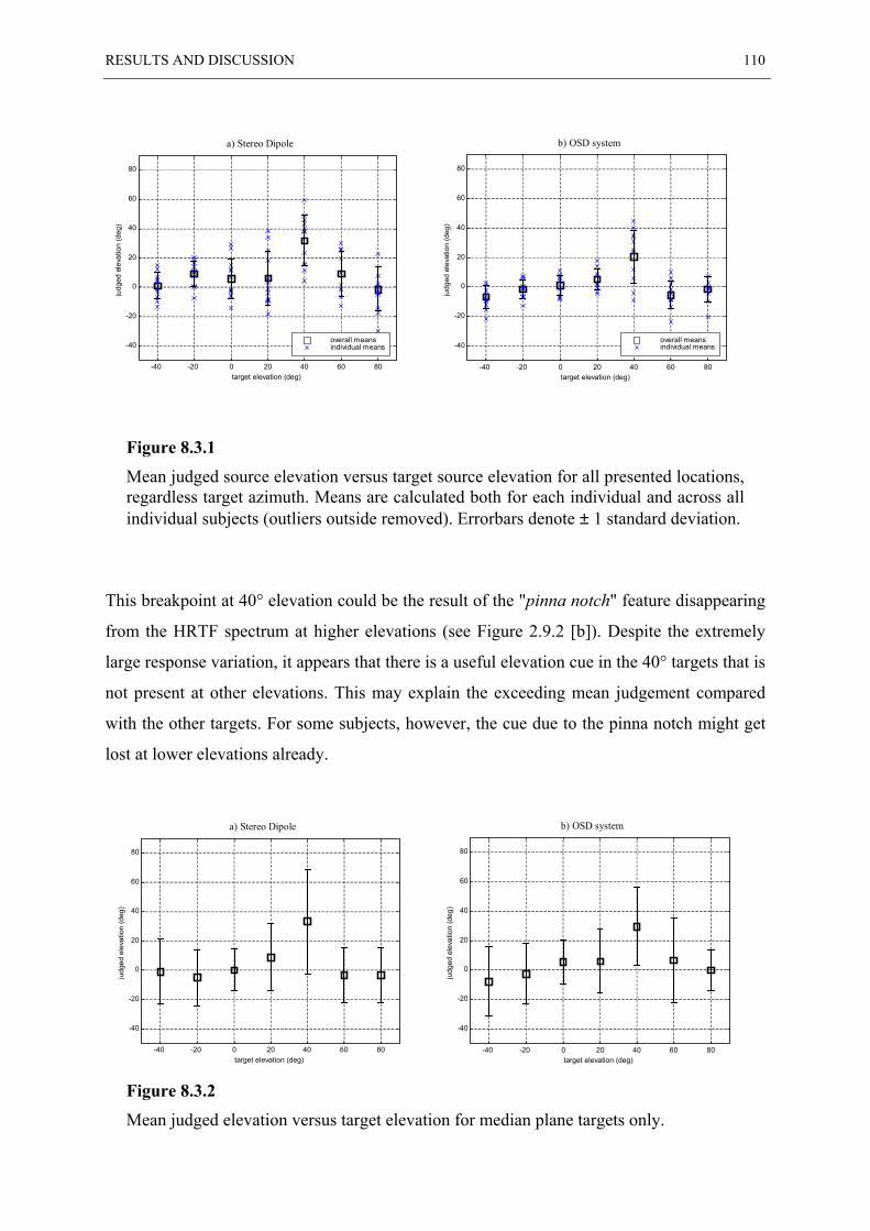
RESULTS AND DISCUSSION 110
b) OSD system
a) Stereo DipoleFigure 8.3.1
Mean judged source elevation versus target source elevation for all presented locations,regardless target azimuth. Means are calculated both for each individual and across allindividual subjects (outliers outside removed). Errorbars denote ± 1 standard deviation.
This breakpoint at 40° elevation could be the result of the "pinna notch" feature disappearing
from the HRTF spectrum at higher elevations (see Figure 2.9.2 [b]). Despite the extremely
large response variation, it appears that there is a useful elevation cue in the 40° targets that is
not present at other elevations. This may explain the exceeding mean judgement compared
with the other targets. For some subjects, however, the cue due to the pinna notch might get
lost at lower elevations already.
-40 -20 0 20 40 60 80
-40
-20
0
20
40
60
80
target elevation (deg)
judg
ed e
leva
tion
(deg
)
overall meansindividual means
-40 -20 0 20 40 60 80
-40
-20
0
20
40
60
80
target elevation (deg)
judg
ed e
leva
tion
(deg
)
overall meansindividual means
b) OSD system
a) Stereo DipoleFigure 8.3.2
Mean judged elevation versus target elevation for median plane targets only.
-40 -20 0 20 40 60 80
-40
-20
0
20
40
60
80
target elevation (deg)
judg
ed e
leva
tion
(deg
)
-40 -20 0 20 40 60 80
-40
-20
0
20
40
60
80
target elevation (deg)
judg
ed e
leva
tion
(deg
)
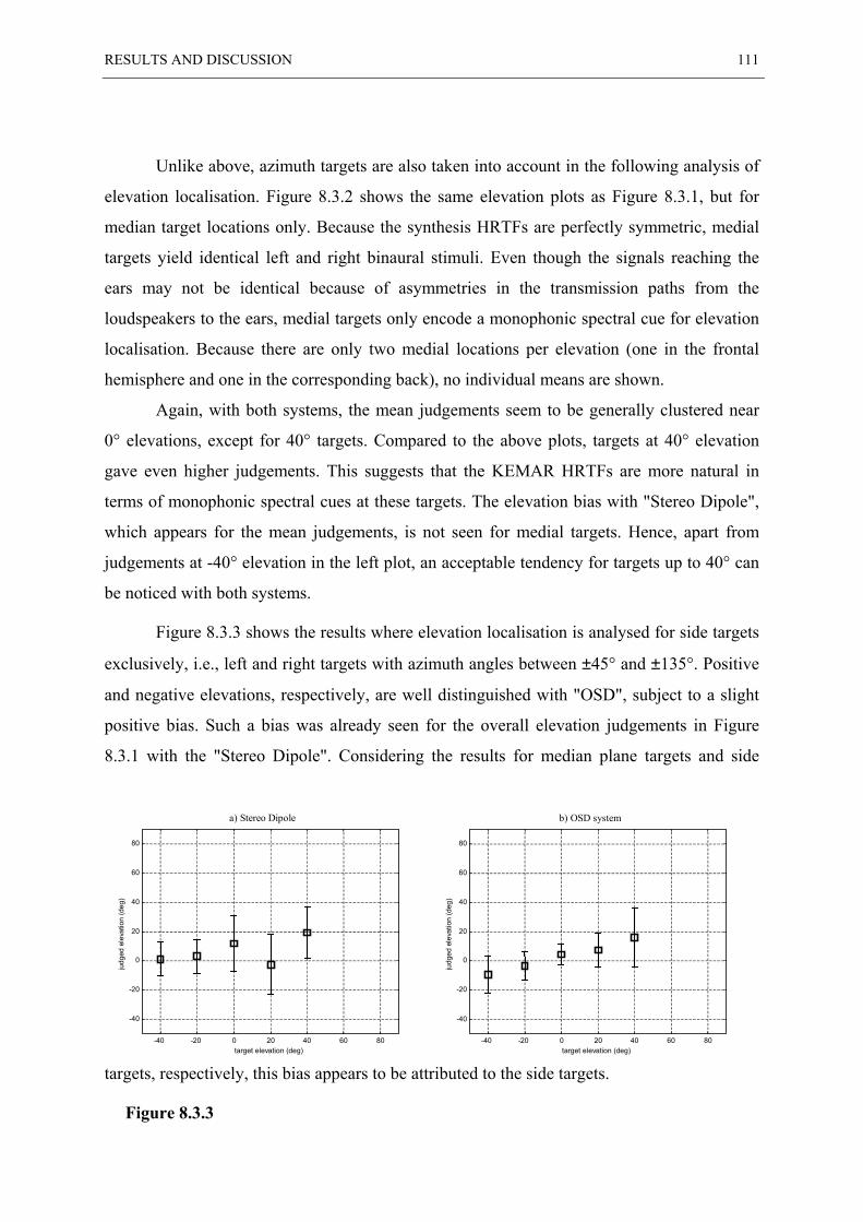
RESULTS AND DISCUSSION 111
Unlike above, azimuth targets are also taken into account in the following analysis of
elevation localisation. Figure 8.3.2 shows the same elevation plots as Figure 8.3.1, but for
median target locations only. Because the synthesis HRTFs are perfectly symmetric, medial
targets yield identical left and right binaural stimuli. Even though the signals reaching the
ears may not be identical because of asymmetries in the transmission paths from the
loudspeakers to the ears, medial targets only encode a monophonic spectral cue for elevation
localisation. Because there are only two medial locations per elevation (one in the frontal
hemisphere and one in the corresponding back), no individual means are shown.
Again, with both systems, the mean judgements seem to be generally clustered near
0° elevations, except for 40° targets. Compared to the above plots, targets at 40° elevation
gave even higher judgements. This suggests that the KEMAR HRTFs are more natural in
terms of monophonic spectral cues at these targets. The elevation bias with "Stereo Dipole",
which appears for the mean judgements, is not seen for medial targets. Hence, apart from
judgements at -40° elevation in the left plot, an acceptable tendency for targets up to 40° can
be noticed with both systems.
Figure 8.3.3 shows the results where elevation localisation is analysed for side targets
exclusively, i.e., left and right targets with azimuth angles between ±45° and ±135°. Positive
and negative elevations, respectively, are well distinguished with "OSD", subject to a slight
positive bias. Such a bias was already seen for the overall elevation judgements in Figure
8.3.1 with the "Stereo Dipole". Considering the results for median plane targets and side
b) OSD system
a) Stereo Dipoletargets, respectively, this bias appears to be attributed to the side targets.
Figure 8.3.3
-40 -20 0 20 40 60 80
-40
-20
0
20
40
60
80
target elevation (deg)
judg
ed e
leva
tion
(deg
)
-40 -20 0 20 40 60 80
-40
-20
0
20
40
60
80
target elevation (deg)
judg
ed e
leva
tion
(deg
)
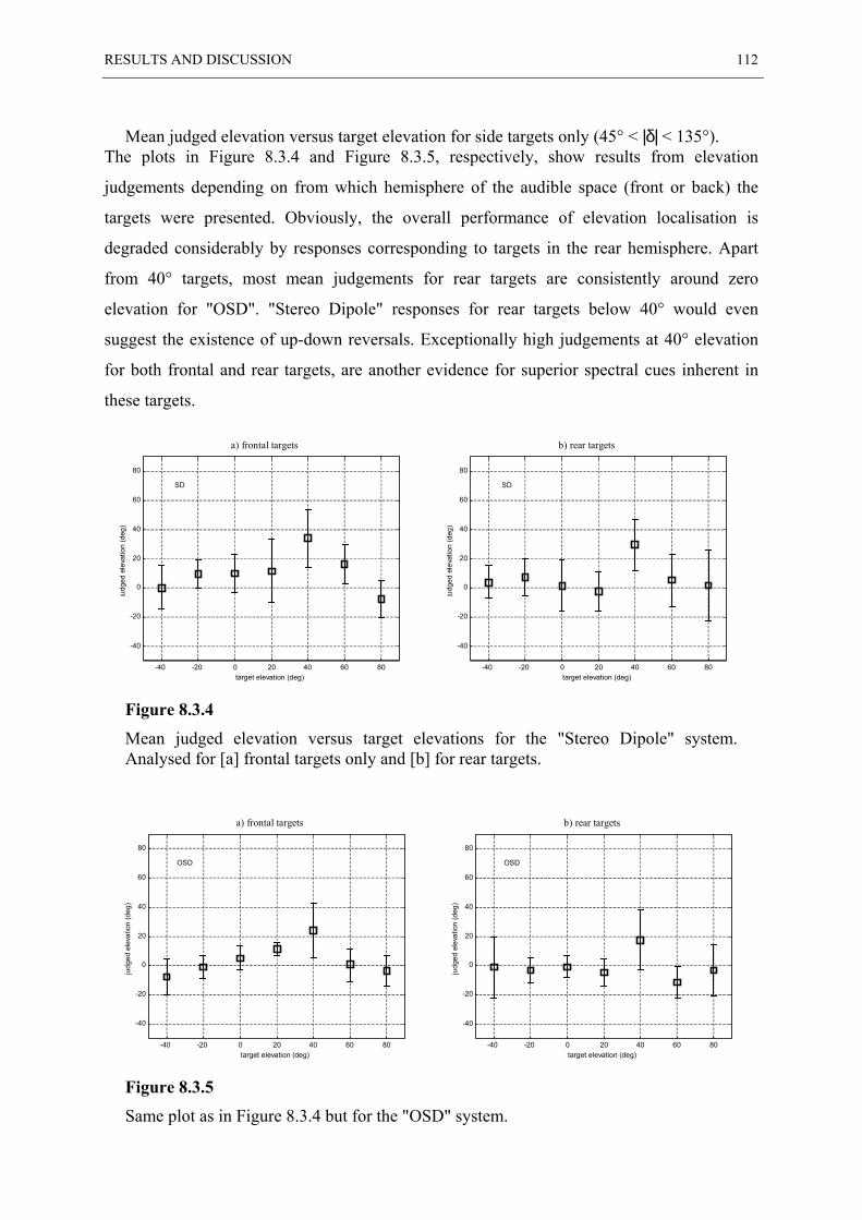
RESULTS AND DISCUSSION 112
Mean judged elevation versus target elevation for side targets only (45° < |δ| < 135°).The plots in Figure 8.3.4 and Figure 8.3.5, respectively, show results from elevation
judgements depending on from which hemisphere of the audible space (front or back) the
targets were presented. Obviously, the overall performance of elevation localisation is
degraded considerably by responses corresponding to targets in the rear hemisphere. Apart
from 40° targets, most mean judgements for rear targets are consistently around zero
elevation for "OSD". "Stereo Dipole" responses for rear targets below 40° would even
suggest the existence of up-down reversals. Exceptionally high judgements at 40° elevation
for both frontal and rear targets, are another evidence for superior spectral cues inherent in
these targets.
Figure 8.3.4
Mean judged elevation versus target elevations for the "Stereo Dipole" system.Analysed for [a] frontal targets only and [b] for rear targets.
b) rear targets
-40 -20 0 20 40 60 80
-40
-20
0
20
40
60
80
target elevation (deg)
judg
ed e
leva
tion
(deg
)
SD
-40 -20 0 20 40 60 80
-40
-20
0
20
40
60
80
b) rear targets
target elevation (deg)
judg
ed e
leva
tion
(deg
)
SD
a) frontal targets
a) frontal targets
Figure 8.3.5
Same plot as in Figure 8.3.4 but for the "OSD" system.
-40 -20 0 20 40 60 80
-40
-20
0
20
40
60
80
target elevation (deg)
judg
ed e
leva
tion
(deg
)
OSD
-40 -20 0 20 40 60 80
-40
-20
0
20
40
60
80
target elevation (deg)
judg
ed e
leva
tion
(deg
)
OSD
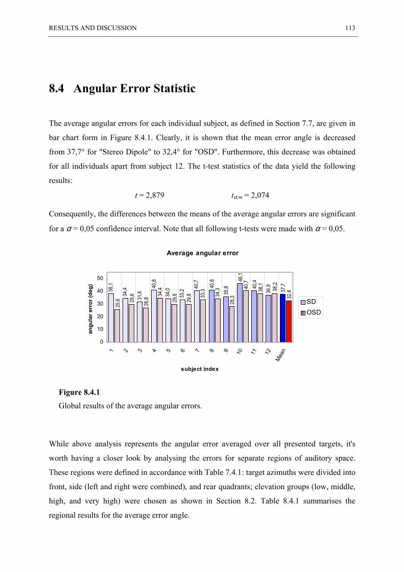
RESULTS AND DISCUSSION 113
8.4 Angular Error Statistic
The average angular errors for each individual subject, as defined in Section 7.7, are given in
bar chart form in Figure 8.4.1. Clearly, it is shown that the mean error angle is decreased
from 37,7° for "Stereo Dipole" to 32,4° for "OSD". Furthermore, this decrease was obtained
for all individuals apart from subject 12. The t-test statistics of the data yield the following
results:
t = 2,879 tα,m = 2,074
Consequently, the differences between the means of the average angular errors are significant
for a α = 0,05 confidence interval. Note that all following t-tests were made with α = 0,05.
Figure 8.4.1
Global results of the average angular errors.
While above analysis represents the angular error averaged over all presented targets, it's
worth having a closer look by analysing the errors for separate regions of auditory space.
These regions were defined in accordance with Table 7.4.1: target azimuths were divided into
front, side (left and right were combined), and rear quadrants; elevation groups (low, middle,
high, and very high) were chosen as shown in Section 8.2. Table 8.4.1 summarises the
regional results for the average error angle.
Average angular error
34,4
34,0
33,2
40,7
40,8
31,638
,1
35,8 36,9
37,740
,446,1
40,8
29,8
29,834
,4
26,829
,6
25,6
33,3 38
,2
32,438
,140,7
34,3
28,3
0
10
20
30
40
50
1 2 3 4 5 6 7 8 9 10 11 12M
ean
subject index
angu
lar e
rror
(deg
)
SDOSD
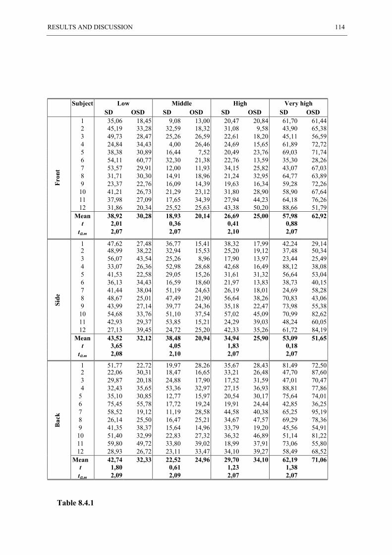
RESULTS AND DISCUSSION 114
Subject Low Middle High Very highSD OSD SD OSD SD OSD SD OSD
1 35,06 18,45 9,08 13,00 20,47 20,84 61,70 61,442 45,19 33,28 32,59 18,32 31,08 9,58 43,90 65,383 49,73 28,47 25,26 26,59 22,61 18,20 45,11 56,594 24,84 34,43 4,00 26,46 24,69 15,65 61,89 72,725 38,38 30,89 16,44 7,52 20,49 23,76 69,03 71,746 54,11 60,77 32,30 21,38 22,76 13,59 35,30 28,267 53,57 29,91 12,00 11,93 34,15 25,82 43,07 67,038 31,71 30,30 14,91 18,96 21,24 32,95 64,77 63,899 23,37 22,76 16,09 14,39 19,63 16,34 59,28 72,26
10 41,21 26,73 21,29 23,12 31,80 28,90 58,90 67,6411 37,98 27,09 17,65 34,39 27,94 44,23 64,18 76,2612 31,86 20,34 25,52 25,63 43,38 50,20 88,66 51,79
Mean 38,92 30,28 18,93 20,14 26,69 25,00 57,98 62,92t 2,01 0,36 0,41 0,88
tα,m 2,07 2,07 2,10 2,07
Fron
t
1 47,62 27,48 36,77 15,41 38,32 17,99 42,24 29,142 48,99 38,22 32,94 15,53 25,20 19,12 37,48 50,343 56,07 43,54 25,26 8,96 17,90 13,97 23,44 25,494 33,07 26,36 52,98 28,68 42,68 16,49 88,12 38,085 41,53 22,58 29,05 15,26 31,61 31,32 56,64 53,046 36,13 34,43 16,59 18,60 21,97 13,83 38,73 40,157 41,44 38,04 51,19 24,63 26,19 18,01 24,69 58,288 48,67 25,01 47,49 21,90 56,64 38,26 70,83 43,069 43,99 27,14 39,77 24,36 35,18 22,47 73,98 55,38
10 54,68 33,76 51,10 37,54 57,02 45,09 70,99 82,6211 42,93 29,37 53,85 15,21 24,29 39,03 48,24 60,0512 27,13 39,45 24,72 25,20 42,33 35,26 61,72 84,19
Mean 43,52 32,12 38,48 20,94 34,94 25,90 53,09 51,65t 3,65 4,05 1,83 0,18
tα,m 2,08 2,10 2,07 2,07
Side
1 51,77 22,72 19,97 28,26 35,67 28,43 81,49 72,502 22,06 30,31 18,47 16,65 33,21 26,48 47,70 87,603 29,87 20,18 24,88 17,90 17,52 31,59 47,01 70,474 32,43 35,65 53,36 32,97 27,15 36,93 88,81 77,86
5 35,10 30,85 12,77 15,97 20,54 30,17 75,64 74,016 75,45 55,78 17,72 19,24 19,91 24,44 42,85 36,257 58,52 19,12 11,19 28,58 44,58 40,38 65,25 95,198 26,14 25,50 16,47 25,21 34,67 47,57 69,29 78,369 41,35 38,37 15,64 14,96 33,79 19,20 45,56 54,91
10 51,40 32,99 22,83 27,32 36,32 46,89 51,14 81,2211 59,80 49,72 33,80 39,02 18,99 37,91 73,06 55,8012 28,93 26,72 23,11 33,47 34,10 39,27 58,49 68,52
Mean 42,74 32,33 22,52 24,96 29,70 34,10 62,19 71,06t 1,80 0,61 1,23 1,38
Bac
k
tα,m 2,09 2,09 2,07 2,07
Table 8.4.1
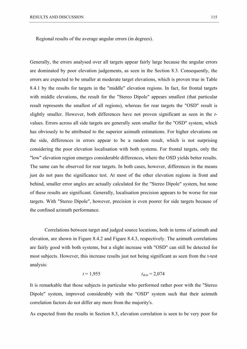
RESULTS AND DISCUSSION 115
Regional results of the average angular errors (in degrees).
Generally, the errors analysed over all targets appear fairly large because the angular errors
are dominated by poor elevation judgements, as seen in the Section 8.3. Consequently, the
errors are expected to be smaller at moderate target elevations, which is proven true in Table
8.4.1 by the results for targets in the "middle" elevation regions. In fact, for frontal targets
with middle elevations, the result for the "Stereo Dipole" appears smallest (that particular
result represents the smallest of all regions), whereas for rear targets the "OSD" result is
slightly smaller. However, both differences have not proven significant as seen in the t-
values. Errors across all side targets are generally seen smaller for the "OSD" system, which
has obviously to be attributed to the superior azimuth estimations. For higher elevations on
the side, differences in errors appear to be a random result, which is not surprising
considering the poor elevation localisation with both systems. For frontal targets, only the
"low" elevation region emerges considerable differences, where the OSD yields better results.
The same can be observed for rear targets. In both cases, however, differences in the means
just do not pass the significance test. At most of the other elevation regions in front and
behind, smaller error angles are actually calculated for the "Stereo Dipole" system, but none
of these results are significant. Generally, localisation precision appears to be worse for rear
targets. With "Stereo Dipole", however, precision is even poorer for side targets because of
the confined azimuth performance.
Correlations between target and judged source locations, both in terms of azimuth and
elevation, are shown in Figure 8.4.2 and Figure 8.4.3, respectively. The azimuth correlations
are fairly good with both systems, but a slight increase with "OSD" can still be detected for
most subjects. However, this increase results just not being significant as seen from the t-test
analysis:
t = 1,955 tα,m = 2,074
It is remarkable that those subjects in particular who performed rather poor with the "Stereo
Dipole" system, improved considerably with the "OSD" system such that their azimuth
correlation factors do not differ any more from the majority's.
As expected from the results in Section 8.3, elevation correlation is seen to be very poor for
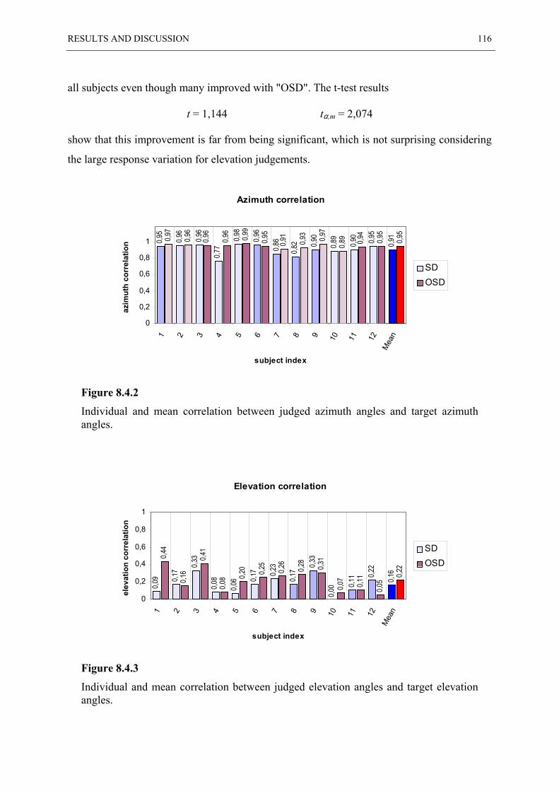
RESULTS AND DISCUSSION 116
all subjects even though many improved with "OSD". The t-test results
t = 1,144 tα,m = 2,074
show that this improvement is far from being significant, which is not surprising considering
the large response variation for elevation judgements.
Figure 8.4.2
Individual and mean correlation between judged azimuth angles and target azimuthangles.
Figure 8.4.3
Individual and mean correlation between judged elevation angles and target elevationangles.
Azimuth correlation
0,95
0,96
0,96
0,77
0,98
0,96
0,86
0,82 0,9
0
0,89
0,90 0,95
0,910,9
7
0,96
0,96
0,96
0,99
0,95
0,91
0,93 0,97
0,89 0,9
4
0,95
0,95
0
0,2
0,4
0,6
0,8
1
1 2 3 4 5 6 7 8 9 10 11 12M
ean
subject index
azim
uth
corr
elat
ion
SDOSD
Elevation correlation
0,09 0,1
7 0,33
0,08
0,06 0,1
7 0,23
0,17 0,3
3
0,11 0,2
2
0,16
0,44
0,16
0,41
0,08 0,2
0 0,25
0,26
0,28
0,31
0,07
0,11
0,05
0,22
0,00
0
0,2
0,4
0,6
0,8
1
1 2 3 4 5 6 7 8 9 10 11 12M
ean
subject index
elev
atio
n co
rrel
atio
n
SDOSD
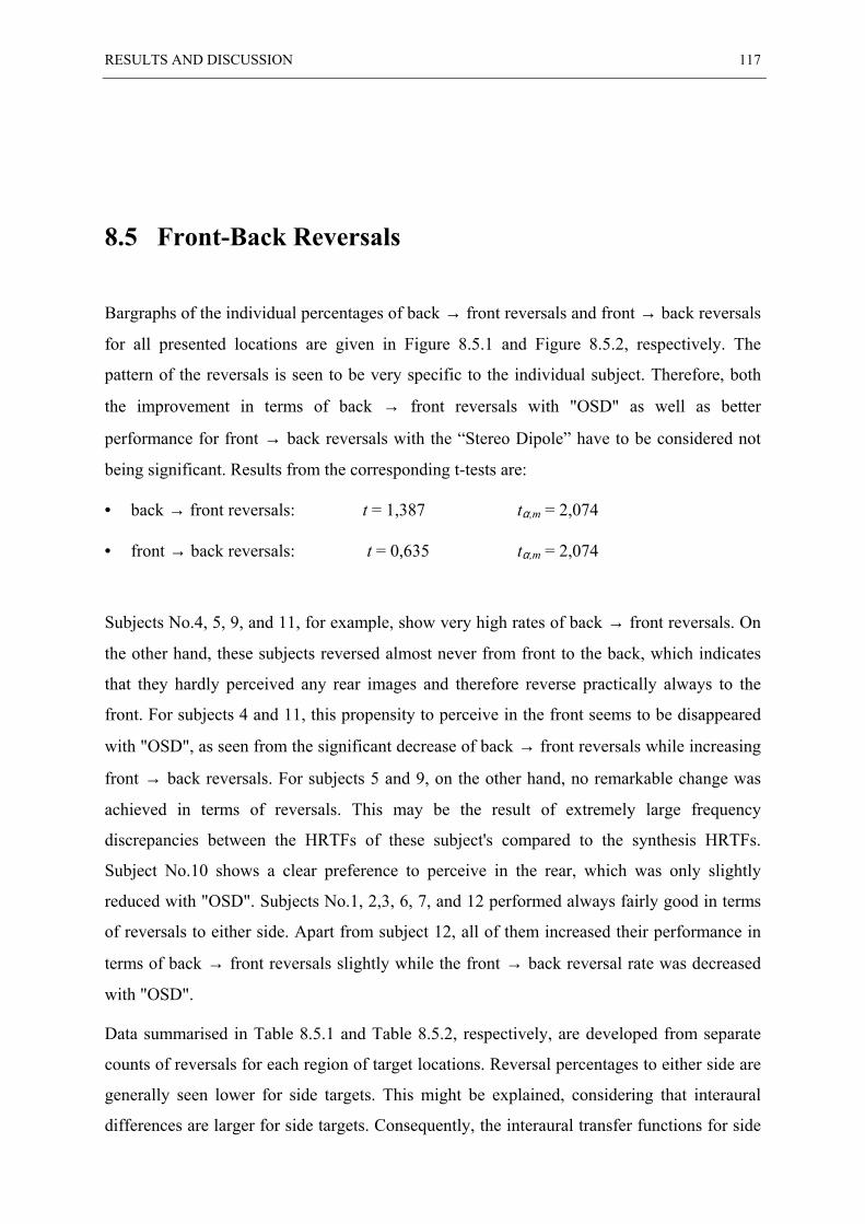
RESULTS AND DISCUSSION 117
8.5 Front-Back Reversals
Bargraphs of the individual percentages of back → front reversals and front → back reversals
for all presented locations are given in Figure 8.5.1 and Figure 8.5.2, respectively. The
pattern of the reversals is seen to be very specific to the individual subject. Therefore, both
the improvement in terms of back → front reversals with "OSD" as well as better
performance for front → back reversals with the “Stereo Dipole” have to be considered not
being significant. Results from the corresponding t-tests are:
• back → front reversals: t = 1,387 tα,m = 2,074
• front → back reversals: t = 0,635 tα,m = 2,074
Subjects No.4, 5, 9, and 11, for example, show very high rates of back → front reversals. On
the other hand, these subjects reversed almost never from front to the back, which indicates
that they hardly perceived any rear images and therefore reverse practically always to the
front. For subjects 4 and 11, this propensity to perceive in the front seems to be disappeared
with "OSD", as seen from the significant decrease of back → front reversals while increasing
front → back reversals. For subjects 5 and 9, on the other hand, no remarkable change was
achieved in terms of reversals. This may be the result of extremely large frequency
discrepancies between the HRTFs of these subject's compared to the synthesis HRTFs.
Subject No.10 shows a clear preference to perceive in the rear, which was only slightly
reduced with "OSD". Subjects No.1, 2,3, 6, 7, and 12 performed always fairly good in terms
of reversals to either side. Apart from subject 12, all of them increased their performance in
terms of back → front reversals slightly while the front → back reversal rate was decreased
with "OSD".
Data summarised in Table 8.5.1 and Table 8.5.2, respectively, are developed from separate
counts of reversals for each region of target locations. Reversal percentages to either side are
generally seen lower for side targets. This might be explained, considering that interaural
differences are larger for side targets. Consequently, the interaural transfer functions for side
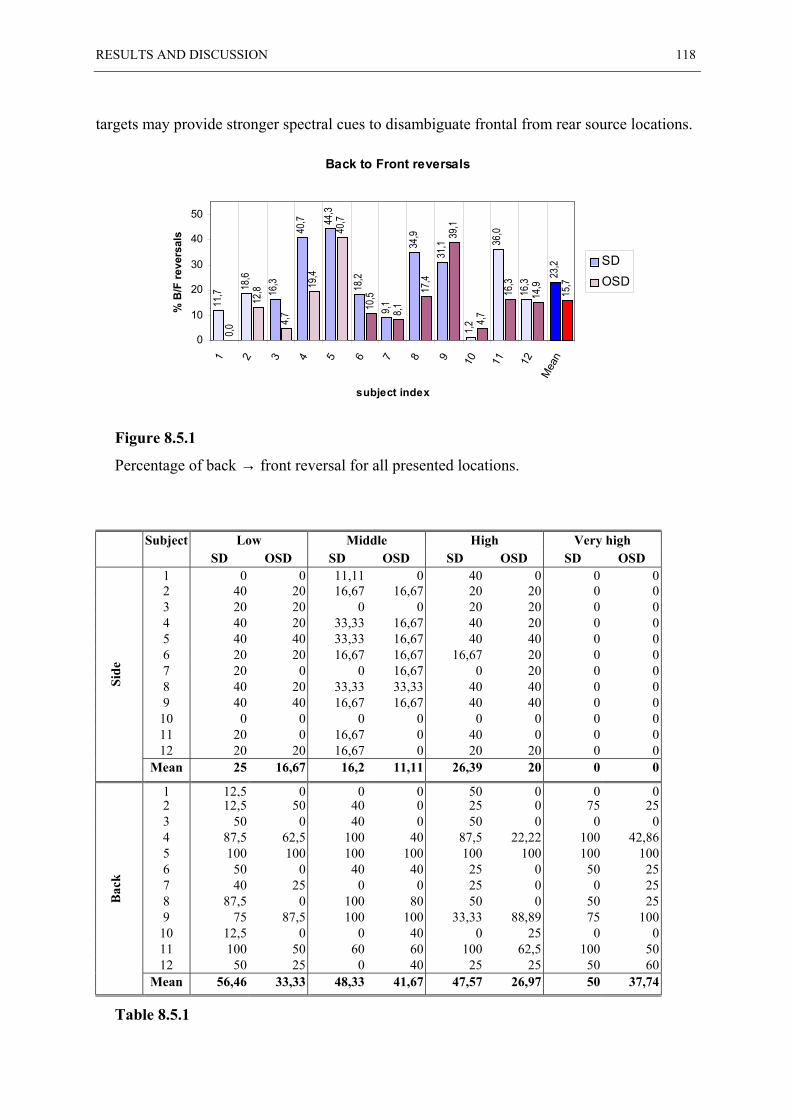
RESULTS AND DISCUSSION 118
targets may provide stronger spectral cues to disambiguate frontal from rear source locations.
Figure 8.5.1
Percentage of back → front reversal for all presented locations.
Subject Low Middle High Very highSD OSD SD OSD SD OSD SD OSD
1 0 0 11,11 0 40 0 0 02 40 20 16,67 16,67 20 20 0 03 20 20 0 0 20 20 0 04 40 20 33,33 16,67 40 20 0 05 40 40 33,33 16,67 40 40 0 06 20 20 16,67 16,67 16,67 20 0 07 20 0 0 16,67 0 20 0 08 40 20 33,33 33,33 40 40 0 09 40 40 16,67 16,67 40 40 0 0
10 0 0 0 0 0 0 0 011 20 0 16,67 0 40 0 0 012 20 20 16,67 0 20 20 0 0
Mean 25 16,67 16,2 11,11 26,39 20 0 0
Side
1 12,5 0 0 0 50 0 0 02 12,5 50 40 0 25 0 75 253 50 0 40 0 50 0 0 04 87,5 62,5 100 40 87,5 22,22 100 42,865 100 100 100 100 100 100 100 1006 50 0 40 40 25 0 50 257 40 25 0 0 25 0 0 258 87,5 0 100 80 50 0 50 259 75 87,5 100 100 33,33 88,89 75 100
10 12,5 0 0 40 0 25 0 011 100 50 60 60 100 62,5 100 5012 50 25 0 40 25 25 50 60
Mean 56,46 33,33 48,33 41,67 47,57 26,97 50 37,74
Bac
k
Table 8.5.1
Back to Front reversals
11,7 18
,6
16,3
40,7 44
,3
18,2
9,1
34,9
31,1
1,2
36,0
16,3
23,2
0,0
12,8
4,7
19,4
40,7
10,5
8,1
17,4
39,1
4,7
16,3
14,9
15,7
0
10
20
30
40
501 2 3 4 5 6 7 8 9 10 11 12
Mea
n
subject index
% B
/F re
vers
als
SDOSD
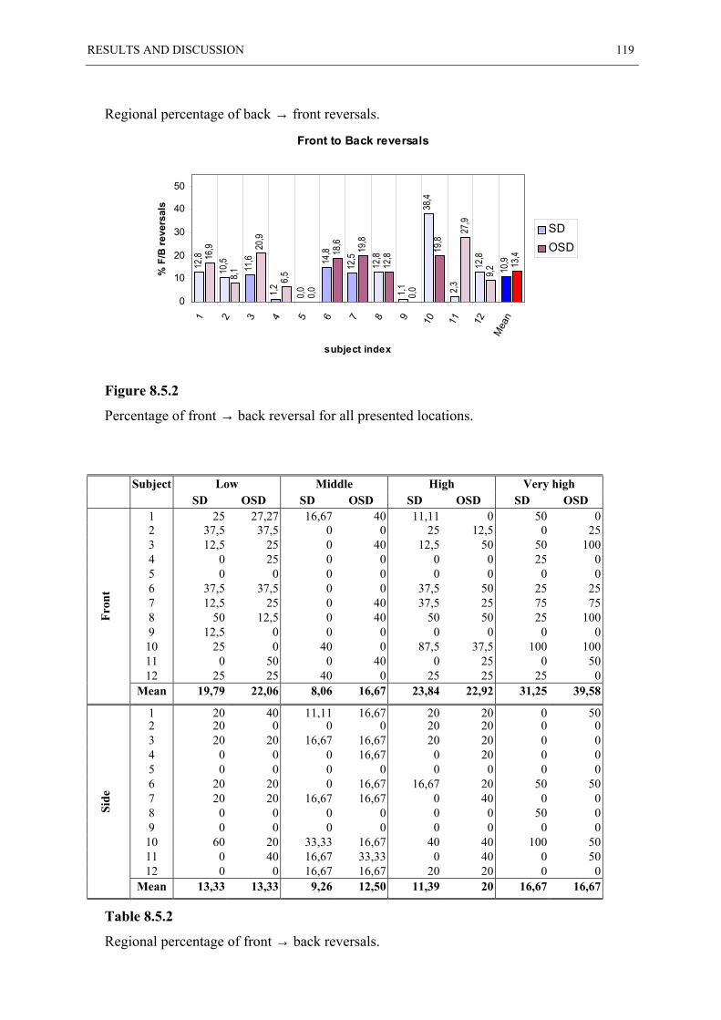
RESULTS AND DISCUSSION 119
Regional percentage of back → front reversals.
Figure 8.5.2
Percentage of front → back reversal for all presented locations.
Subject Low Middle High Very highSD OSD SD OSD SD OSD SD OSD
1 25 27,27 16,67 40 11,11 0 50 02 37,5 37,5 0 0 25 12,5 0 253 12,5 25 0 40 12,5 50 50 1004 0 25 0 0 0 0 25 05 0 0 0 0 0 0 0 06 37,5 37,5 0 0 37,5 50 25 257 12,5 25 0 40 37,5 25 75 758 50 12,5 0 40 50 50 25 1009 12,5 0 0 0 0 0 0 0
10 25 0 40 0 87,5 37,5 100 10011 0 50 0 40 0 25 0 5012 25 25 40 0 25 25 25 0
Mean 19,79 22,06 8,06 16,67 23,84 22,92 31,25 39,58
Fron
t
1 20 40 11,11 16,67 20 20 0 502 20 0 0 0 20 20 0 03 20 20 16,67 16,67 20 20 0 04 0 0 0 16,67 0 20 0 05 0 0 0 0 0 0 0 06 20 20 0 16,67 16,67 20 50 507 20 20 16,67 16,67 0 40 0 08 0 0 0 0 0 0 50 09 0 0 0 0 0 0 0 0
10 60 20 33,33 16,67 40 40 100 5011 0 40 16,67 33,33 0 40 0 5012 0 0 16,67 16,67 20 20 0 0
Mean 13,33 13,33 9,26 12,50 11,39 20 16,67 16,67
Side
Table 8.5.2
Regional percentage of front → back reversals.
Front to Back reversals
12,8
10,5 11,6
1,2 0,0
14,8
12,5
12,8
1,1
38,4
2,3
12,8
10,916
,9
8,1
20,9
6,5
0,0
18,6 19,8
12,8
0,0
19,8
27,9
9,2
13,4
0
10
20
30
40
501 2 3 4 5 6 7 8 9 10 11 12
Mea
n
subject index
% F
/B re
vers
als
SDOSD
RESULTS AND DISCUSSION 120
It is remarkable that for very high elevations on the side, none of the subjects reversed to the
front while some located frontal targets in the rear. However, considering that only a few
targets corresponding to this region were actually presented, this result should be handled
with care. With both systems, highest reversal rates resulted for rear targets at all elevations,
which were located at the front. Subjects who perceive preferably at the front seem to be
more common and they make their judgements more consistently. This is seen from some
subjects who show 100% back → front reversals for almost all target elevations around the
median plane. Despite some weak indications, due to the large individual variations related to
reversals, it is fairly difficult to trace a significant difference between the investigated
systems.
8.6 Concluding Remarks
This study has discussed how loudspeaker binaural audio systems can be practically
implemented as “multi-way” systems. Such systems are referred to as “Optimal Source
Distribution”, or “OSD” systems. It was shown that such systems are well-behaving in terms
of acoustic transmission path inversion (crosstalk cancellation) over a wide frequency range.
As a consequence, “OSD” systems are capable to create very convincing virtual images in a
3D listening space. Results of subjective sound localisation experiments confirmed some
remarkable improvements compared to a conventional “Stereo Dipole” system, which uses a
pair of closely spaced transducers over the whole reproduced frequency range. The most
significant improvement is seen as a respectable widening of the range of perceived azimuth
angles towards lateral source locations. While cones of confusions at azimuth angles within
approximately ± 45° were recognised reasonably well with the “Stereo Dipole” system, the
“OSD” system yielded a range of almost ± 70°.
Moreover, obtained results generally appear more reliable with the “OSD” system,
considering the much smaller response variation between subjects. This was also seen for
elevation judgements, even though performance in terms of elevation localisation was rather
RESULTS AND DISCUSSION 121
poor for both systems. In general, elevation localisation is difficult to test due to the large
variation in the responses, contrary to azimuth localisation. It is known from experiments
with real sound sources that the just noticeable difference (JND) of elevation is relatively
large [Blauert, 1997]. Never the less, for target elevations within ± 40°, reasonably consistent
results for the “OSD” system still suggest improved accuracy of elevation localisation.
Average angular error calculations can be considered as an analysis of localisation
precision in a three-dimensional sense. Over all presented target locations, this performance
was significantly improved with the “OSD” system. However, separate investigations for
particular regions of the listening space reveal that this improvement is mainly attributed to
the better performance for side targets. For targets close to the median plane (frontal and
rear), no significant differences in terms of error angles could be found.
The percentage of front-reversals is seen as being very specific to the individual
subject. Therefore, significant differences between the two systems must be considered
influenced by other factors, such as match of synthesis HRTFs with the subjects HRTFs.
A procedural disadvantage of the localisation tests might be the fact that all target
locations were presented only once per subject with each system. As a consequence, response
variation was fairly large which makes it difficult in some cases to draw reliable conclusions
out of the results. With the hypothesis that interindividual variance is generally larger than
intraindividual variance, this lack of reproducibility could have had alleviated. Considering
time schedules for the experiments, the experimenter had accept this compromise. Otherwise,
less targets had to be presented if one wants to avoid increasing the duration of the test
sessions.
Objectives for future work in this area could be to test more practical systems. Since
virtual acoustic systems based on binaural reproduction are still fairly sensitive to listener
position, a major application of them is in the field of desktop applications, such as
computers, video games, or cars. Hence, a 3-way system as it was designed here, (with low-
frequency speakers span of 180°) will not be practically for many of those applications.
Consequently, systems which require less space appear to be of more interest. This could be
realised in 2-way or in 3-way with smaller loudspeaker span for the woofers. According to
Takeuchi and Nelson [2000a; 2000b], in theory the woofer span could be considerably
reduced without remarkable changes of the low-frequency limit with crosstalk cancellation
(see Section 5.8).
RESULTS AND DISCUSSION 122
Another challenge will be to realise transducers, which in reality change their span as a
function of frequency. As proposed by Takeuchi and Nelson [2000a], this might, for
example, be realised by exciting a triangular shaped plate whose width varies along its
length. The requirement of such a transducer is that a certain frequency of vibration is excited
most at a particular position having a certain width such that sound of that frequency is
radiated mostly from that position.

Bibliography
AES (1986), edited by Eargle, J.M., Stereophonic Techniques, The Audio Engineering
Society, New York, 1986.
Atal, B.S., M. Hill, M.R. Schroeder (1966), Apparent Sound Source Translator, United
States Patent Office, No. 3,236,949 (22 February 1966).
Bauck, J.L., and D.H. Cooper (1996), Generalised Transaural Stereo and Applications, J.
Audio Eng. Soc., Vol. 44, No. 9, pp. 683-705.
Bauer, B.B. (1961), Stereophonic Earphones and Binaural Loudspeakers, J. Audio Eng.
Soc., Vol. 9, No.2, pp. 148-151.
Begault, D.R. (1992), Perceptual Effects of Synthetic Reverberation on Three-Dimensional
Audio Systems, J. Audio Eng. Soc., Vol. 40, pp. 895-904.
Begault, D.R. (1994), 3-D Sound for Virtual Reality and Multimedia, Academic Press
Professional, ISBN 0-12-084735-3.
Berkhout, A.J., D. de Vries, P. Vogel (1993), Acoustic Control by Wave Field Synthesis, J.
Acoust. Soc. of Am., No. 5, pp. 2764-2778.
Blauert, J. (1997), Spatial Hearing: The Psychophysics of Human Sound Localisation, MIT
Press, ISBN 0-262-02413-6.

BIBLIOGRAPHY 124
Boone, M.M., E. Verheijen, P. Tol (1995), Spatial Sound Field Reproduction by Wave Field
Synthesis, J. Audio Eng. Soc., Vol. 43, No. 12, pp. 1003-1012.
Bronstein, I.N., and K.A. Semendjajew (1996), Teubner-Taschenbuch der Mathematik,
B.G. Teubner, Stuttgart, ISBN 3-8154-2001-6.
Colloms, M., (1997), High Performance Loudspeakers, 5th edition, John Wiley & Sons.
Cooper, D.H., and J.L. Bauck (1989), Prospects for transaural recording, J. Audio Eng.
Soc., Vol. 37, No.1/2, pp. 3-19.
Damaske, P. (1971), Head-Related Two-Channel Stereophony with Loudspeaker
Reproduction, J. Acoust. Soc. of Am., Vol. 50, No. 4, pp. 1109-1115.
Duda, R.O. (1996), 3-D Audio for Human Computer Interface, San Jose State University,
<http://www-engr.sjsu.edu/~knapp/HCIROD3D/3D_home.htm>.
Gardner, W.G., and K.D. Martin (1994), HRTF Measurements of a KEMAR Dummy-Head
Microphone, M.I.T. Media Lab, Perceptual Computing Section, Technical Report No. 280.
<http://sound.media.mit.edu/KEMAR.html>
Gardner, W.G. (1997), 3-D Audio Using Loudspeakers, PhD dissertation, M.I.T. Media
Lab.
Griesinger, D. (1989), Equalisation and Spatial Equalisation of Dummy-Head Recordings
for Loudspeaker Reproduction, J. Audio Eng. Soc., Vol. 37, No.1/2, pp. 20-29.
Hartmann, W.M. (1997), Listening in a Room and the Precedence Effect, in Binaural and
Spatial Hearing in Real and Virtual Environments, ed. R.H. Gilkey and T.R. Anderson,
Lawrence, Erlbaum Associates, ISBN 0-8058-1654-2.
Heegaard, F.D. (1992), The Reproduction of Sound in Auditory Perspective and a
BIBLIOGRAPHY 125
Compatible System of Stereophony, EBU Rev., Pt. A-Technical, No. 50, pp. 2-6 (1958 Dec.);
reprinted in J. Audio Eng. Soc., Vol. 40, No. 10, pp. 802-808.
Kirkeby, O., P.A. Nelson, H. Hamada, F. Orduña-Bustamente (1996a), Fast
Deconvolution of Multi-Channel Systems using Regularisation, ISVR Technical Report, No.
255, Institute of Sound and Vibration Research, University of Southampton.
Kirkeby, O., P.A. Nelson, H. Hamada (1996b), “Stereo Dipole”, British Patent
Application, No. 9603236.2
Kirkeby, O., P.A. Nelson, H. Hamada (1997), The “Stereo Dipole” - Binaural Sound
Reproduction using two closely spaced Loudspeakers, presented at the 102nd Audio
Engineering Society Convention, 22-25 March 1997, Munich, Germany, AES preprint 4463
(I6). Also published in J. Audio Eng. Soc., Vol. 46, No. 5, pp. 387-395 (1998).
Kirkeby, O., and P.A. Nelson (1997), Virtual Source Imaging using the “Stereo Dipole”,
presented at the 103rd Audio Engineering Society Convention, 26-29 September 1997, New
York, AES preprint 4574 (J10).
Kirkeby, O., P.A. Nelson, H. Hamada (1998), Local Sound Field Reproduction using two
closely spaced Loudspeakers, J. Acoust. Soc. of Am., Vol. 104, No. 4, pp. 1973-1981.
Kleiner, M. (1978), Problems in the design and use of “dummy heads”, Acustica, Vol. 41,
pp. 183-193.
Kreyszig, E. (1983), Advanced Engineering Mathematics, John Wiley and Sons.
Møller, H. (1989), Reproduction of Artificial-Head Recordings through Loudspeakers, J.
Audio Eng. Soc., Vol. 37, No.1/2, pp. 30-33.
Møller, H. (1992), Fundamentals of Binaural Technology, Applied Acoustics, Vol. 36, 1992,
pp. 171-218
BIBLIOGRAPHY 126
Møller, H., C.B. Jensen, D. Hammershøi, M.F. Sørensen (1997), Evaluation of artificial
heads in listening tests, presented at the 102nd Audio Engineering Society Convention, 22-25
March 1997, Munich, Germany, AES preprint 4404 (A1).
Nelson, P.A., and S.J. Elliott (1992), Active Control of Sound, Academic Press, London,
ISBN 0-12-515426-7.
Nelson, P.A., H. Hamada, S.J. Elliott (1992), Adaptive Inverse Filters for Stereophonic
Sound Reproduction, IEEE Trans. Signal Process., Vol. 40, No. 7, pp. 1621-1632.
Nelson, P.A., F. Orduña-Bustamente, H. Hamada (1995), Inverse Filter Design and
Equalisation Zones in Multi-Channel Sound Reproduction, IEEE Trans. Speech Audio
Process., Vol. 3, No. 3, pp. 185-192.
Nelson, P.A., and F. Orduña-Bustamente (1996), Multi-Channel Signal Processing
Techniques in the Reproduction of Sound, J. Audio Eng. Soc. Vol. 44, pp. 973-989.
Nelson, P.A., O. Kirkeby, T. Takeuchi, H. Hamada (1997), Sound Fields for the
Production of Virtual Acoustic Images, J. Sound. Vib., Vol. 204, No. 2, pp. 386-396.
Oppenheim A.V., and R.W. Schafer (1975), Digital Signal Processing, Prentice-Hall Inc.,
Englewood Cliffs, NJ, ISBN 0-13-214635-5.
Pierce, A.D. (1981), Acoustics. An Introduction to its Physical Principles and Applications,
McGraw-Hill, New York.
Press, W.H., S.A. Teukolsky, W.T. Vetterling, B.P. Flannery (1992), Numerical Recipes
in C, Second edition, Cambridge University Press.
Proakis, J.G., and D.G. Manolakis (1996), Digital Signal Processing-Principles,
Algorithms, and Applications, 3rd ed. Prentice-Hall Inc., Englewood Cliffs, NJ, ISBN 0-13-
394289-9.

BIBLIOGRAPHY 127
Pulkki, V. (1997), Virtual Sound Source Positioning Using Vector Base Amplitude Panning,
J. Audio Eng. Soc., Vol. 45, No. 6, pp. 944-951.
Rife, D.D., and J.Vanderkooy (1989), Transfer-Function Measurements using Maximum
Length Sequences, J. Audio Eng. Soc., Vol. 37, No. 6, pp. 419-444.
Rife, D.D. (1994), Maximum Length Sequence System Analyser (MLSSA), Reference Manual,
Version 9.0, DRA Laboratories.
Schroeder, M.R., and B.S. Atal (1963), Computer Simulation of Sound Transmission in
Rooms, IEEE Int. Conv. Record, 7, pp. 150-155.
Schroeder, M.R. (1975), Models of Hearing, Proceedings of the IEEE, Vol. 63, No. 9, pp.
1332-1352.
Takeuchi, T., P.A. Nelson, O. Kirkeby, H. Hamada (1997), Robustness of the performance
of the “Stereo Dipole” to misalignment of head position, presented at the 102nd Audio
Engineering Society Convention, 22-25 March 1997, Munich, Germany, AES preprint 4464
(I7).
Takeuchi, T., P.A. Nelson, O. Kirkeby, H. Hamada (1998), Influence of Individual Head
Related Transfer Functions on the Performance of Virtual Acoustic Imaging Systems, 104th
Audio Engineering Society Convention, AES preprint 4700 (P4-3).
Takeuchi, T., and P.A. Nelson (2000a), Optimal Source Distribution for Virtual Acoustic
Imaging, British Patent application, No. 0015419.5
Takeuchi, T., and P.A. Nelson (2000b), Optimal Source Distribution for Virtual Acoustic
Imaging, ISVR Technical Report, No. 288, Institute of Sound and Vibration Research,
University of Southampton.

BIBLIOGRAPHY 128
Vanderkooy, J. (1994), Aspects of MLS Measuring Systems, J. Audio Eng. Soc., Vol. 42,
No. 4, pp. 219-231.
Wenzel, E.M., M. Arruda, D. Kistler, F.L. Wightman (1993), Localisation using
nonindividualised Head-Related Transfer Functions. Prentice-Hall Inc., J. Acoust. Soc. of
Am., Vol. 94, No. 1, pp. 111-123.
Widrow, B., and S.D. Stearns (1985), Adaptive Signal Processing. Prentice-Hall Inc.,
Englewood Cliffs, NJ, ISBN 0-13-004029-0.
Wiener, N. (1949), Extrapolation, Interpolation and Smoothing of Stationary Time Series
with Engineering Applications. Wiley, New York.
Wightman, F.L., and D.J. Kistler (1989a), Headphone Simulation of Free-Field Listening,
I: Stimulus Synthesis, J. Acoust. Soc. of Am., Vol. 85, No. 2, pp. 858-867.
Wightman, F.L., and D.J. Kistler (1989b), Headphone Simulation of Free-Field Listening,
II: Psychophysical Validation, J. Acoust. Soc. of Am., Vol. 85, No. 2, pp. 868-878.
Wilkinson, J.H. (1965), The Algebraic Eigenvalue Problem, Oxford University Press.