Bayesian Scientific Computing, Spring 2013 (N. Zabaras)

Binary Variables, Bernoulli,

Binomial and Multinomial

Distributions

Prof. Nicholas Zabaras

School of Engineering

University of Warwick

Coventry CV4 7AL

United Kingdom

Email: nzabaras@gmail.com

URL: http://www.zabaras.com/

August 7, 2014

1

Bayesian Scientific Computing, Spring 2013 (N. Zabaras)

Binary Variables

Bernoulli distribution, Likelihood, Prior

Binomial distribution, Mean and Variance, Normalization Constant

Multinoulli/Caterogorical Distribution, Multinomial distribution, Biosequence

Analysis Example

Summary of Multinomial Related Discrete Distributions

Poisson Distribution

Empirical Distribution

2

• Following closely Chris Bishops’ PRML book, Chapter 2

• Kevin Murphy’s, Machine Learning: A probablistic perspective, Chapter 2

Contents

Bayesian Scientific Computing, Spring 2013 (N. Zabaras)

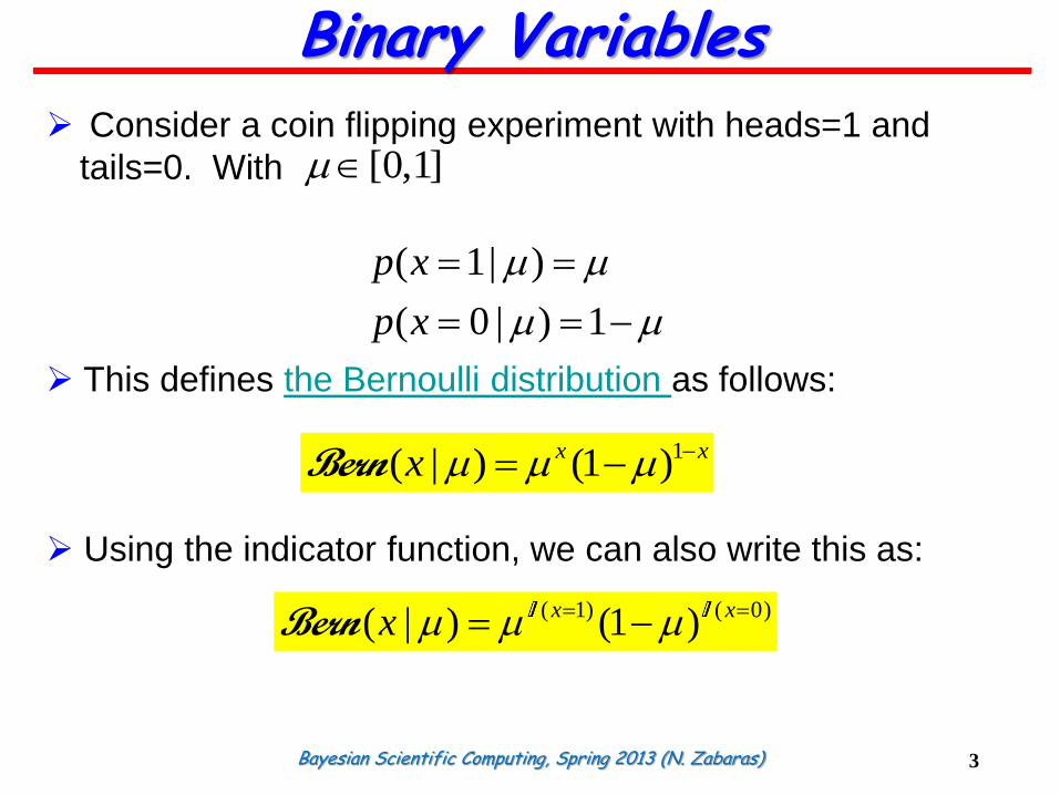
Consider a coin flipping experiment with heads=1 and

tails=0. With

This defines the Bernoulli distribution as follows:

Using the indicator function, we can also write this as:

( 1| )

( 0 | ) 1

p x

p x

Binary Variables

3

[0,1]

1( | ) (1 )x xx Bern

( 1) ( 0)( | ) (1 )x xx Bern

Bayesian Scientific Computing, Spring 2013 (N. Zabaras)

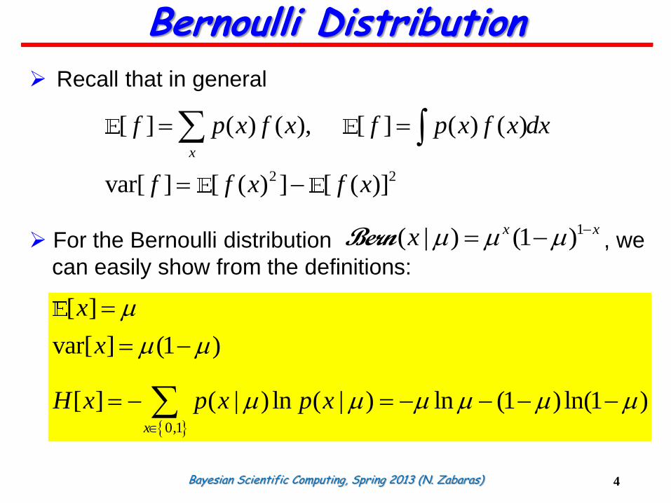
Recall that in general

For the Bernoulli distribution , we

can easily show from the definitions:

2 2

[ ] ( ) ( ), [ ] ( ) ( )

var[ ] [ ( ) ] [ ( )]

x

f p x f x f p x f x dx

f f x f x

Bernoulli Distribution

4

0,1

[ ]

var[ ] (1 )

[ ] ( | ) ln ( | ) ln (1 ) ln(1 )x

x

x

H x p x p x

1( | ) (1 )x xx Bern

Bayesian Scientific Computing, Spring 2013 (N. Zabaras)

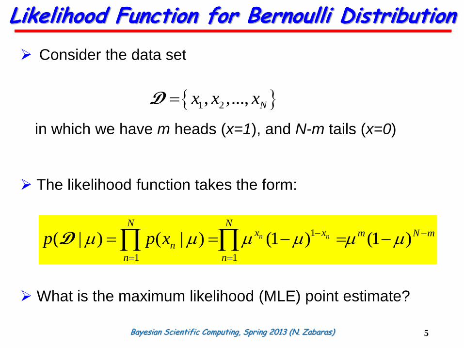
Consider the data set

in which we have m heads (x=1), and N-m tails (x=0)

The likelihood function takes the form:

What is the maximum likelihood (MLE) point estimate?

1 2, ,..., Nx x xD

Likelihood Function for Bernoulli Distribution

5

1

1 1

( | ) ( | ) (1 ) (1 )n n

N Nx x m N m

n

n n

p p x

D

Bayesian Scientific Computing, Spring 2013 (N. Zabaras)

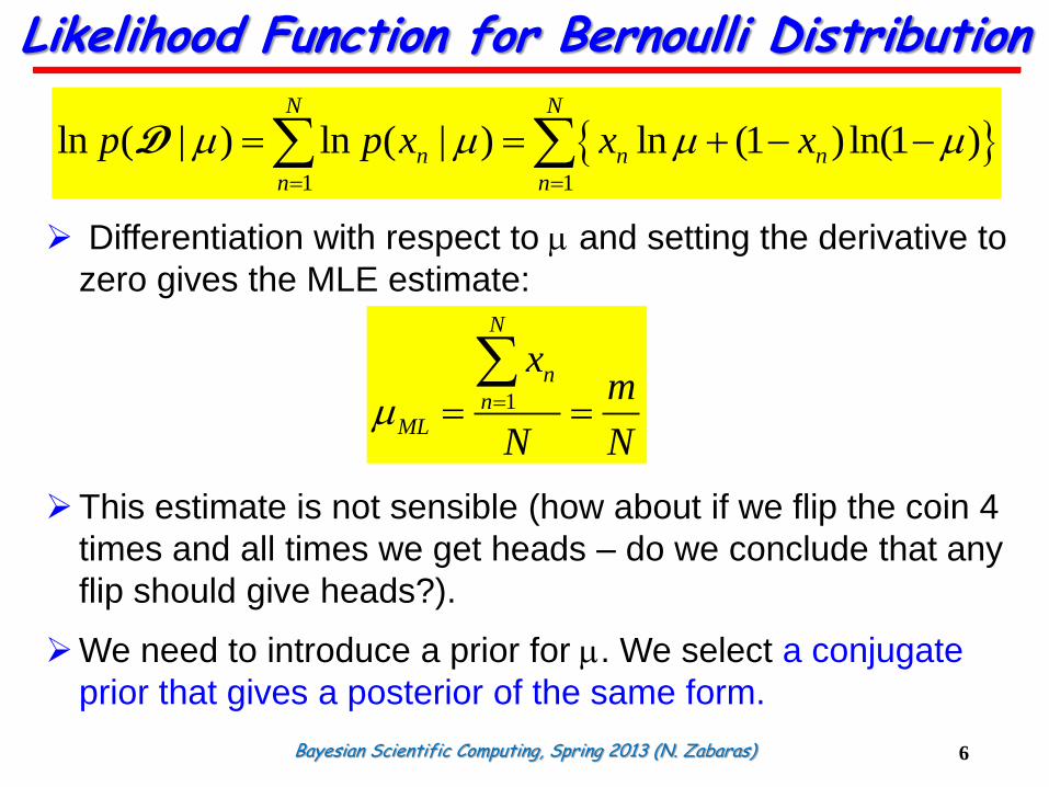
Differentiation with respect to and setting the derivative to

zero gives the MLE estimate:

This estimate is not sensible (how about if we flip the coin 4

times and all times we get heads – do we conclude that any

flip should give heads?).

We need to introduce a prior for . We select a conjugate

prior that gives a posterior of the same form.

Likelihood Function for Bernoulli Distribution

6

1 1

ln ( | ) ln ( | ) ln (1 ) ln(1 )N N

n n n

n n

p p x x x

D

1

N

n

nML

xm

N N

Bayesian Scientific Computing, Spring 2013 (N. Zabaras)

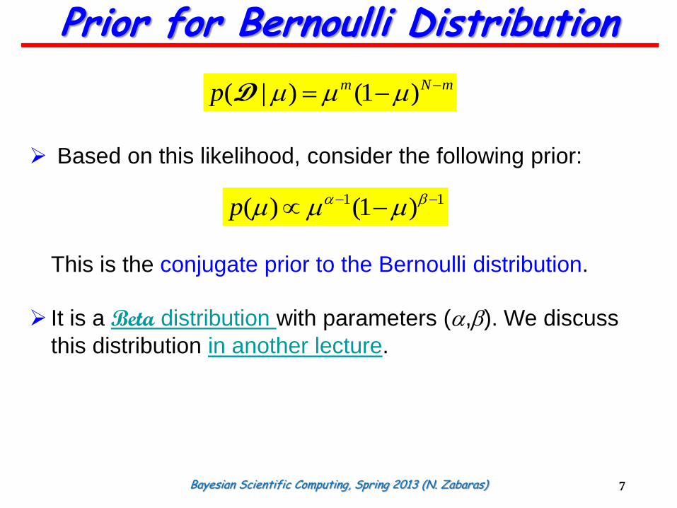
Based on this likelihood, consider the following prior:

This is the conjugate prior to the Bernoulli distribution.

It is a Beta distribution with parameters (a,b). We discuss

this distribution in another lecture.

Prior for Bernoulli Distribution

7

( | ) (1 )m N mp D

1 1( ) (1 )p a b

Bayesian Scientific Computing, Spring 2013 (N. Zabaras)

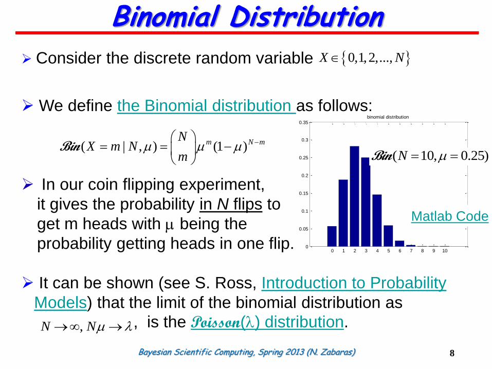
Consider the discrete random variable

We define the Binomial distribution as follows:

In our coin flipping experiment,

it gives the probability in N flips to

get m heads with being the

probability getting heads in one flip.

It can be shown (see S. Ross, Introduction to Probability

Models) that the limit of the binomial distribution as

, is the Poisson(l) distribution.

0,1,2,...,X N

( | , ) (1 )m N mN

X m Nm

Bin

,N N l

Binomial Distribution

8

0 1 2 3 4 5 6 7 8 9 100

0.05

0.1

0.15

0.2

0.25

0.3

0.35binomial distribution

( 10, 0.25)N Bin

Matlab Code

Bayesian Scientific Computing, Spring 2013 (N. Zabaras)

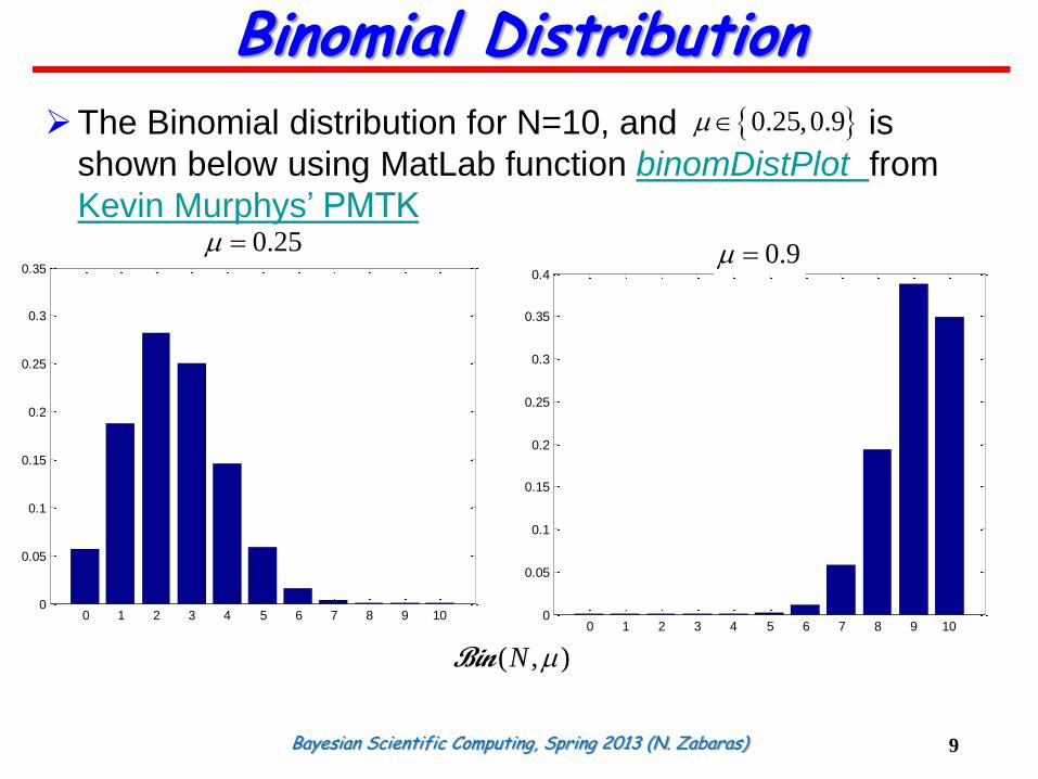
The Binomial distribution for N=10, and is

shown below using MatLab function binomDistPlot from

Kevin Murphys’ PMTK

0.25,0.9

Binomial Distribution

9

( , )N Bin

0 1 2 3 4 5 6 7 8 9 100

0.05

0.1

0.15

0.2

0.25

0.3

0.35=0.250

0 1 2 3 4 5 6 7 8 9 100

0.05

0.1

0.15

0.2

0.25

0.3

0.35

0.4=0.9000.9 0.25

Bayesian Scientific Computing, Spring 2013 (N. Zabaras)

Consider for independent events the mean of the sum is

the sum of the means, and the variance of the sum is the

sum of the variances.

Because m = x1 + . . . + xN, and for each observation the

mean and variance are known from the Bernoulli

distribution:

One can also compute by differentiating

(twice) wrt .

1

0

2

1

0

[ ] ( | , ) [ ... ]

[ ] [ ] ( | , ) [ ... ] (1 )

N

N

m

N

N

m

m m m N x x N

var m m m m N var x x N

Bin

Bin

Mean,Variance of the Binomial Distribution

10

2[ ], [ ]m m

1

(1 ) 1N

m N m

m

N

m

Bayesian Scientific Computing, Spring 2013 (N. Zabaras)

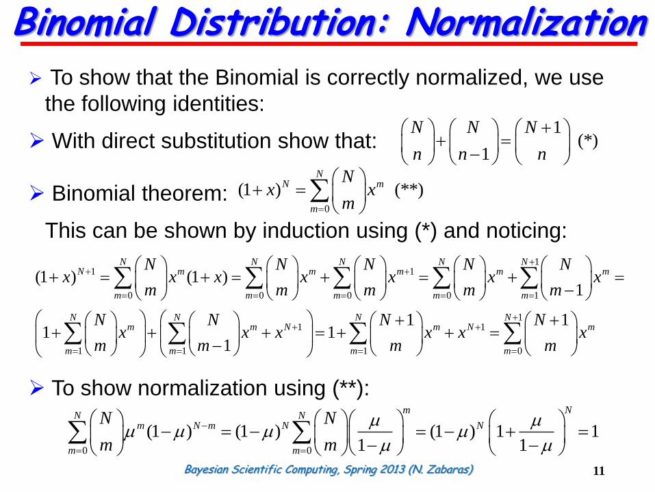
To show that the Binomial is correctly normalized, we use

the following identities:

With direct substitution show that:

Binomial theorem:

This can be shown by induction using (*) and noticing:

To show normalization using (**):

0

(1 ) (**)N

N m

m

Nx x

m

Binomial Distribution: Normalization

11

1(*)

1

N N N

n n n

11 1

0 0 0 0 1

11 1

1 1 1 0

(1 ) (1 )1

1 11 1

1

N N N N NN m m m m m

m m m m m

N N N Nm m N m N m

m m m m

N N N N Nx x x x x x x

m m m m m

N N N Nx x x x x x

m m m m

0 0

(1 ) (1 ) (1 ) 1 11 1

m NN N

m N m N N

m m

N N

m m

Bayesian Scientific Computing, Spring 2013 (N. Zabaras)

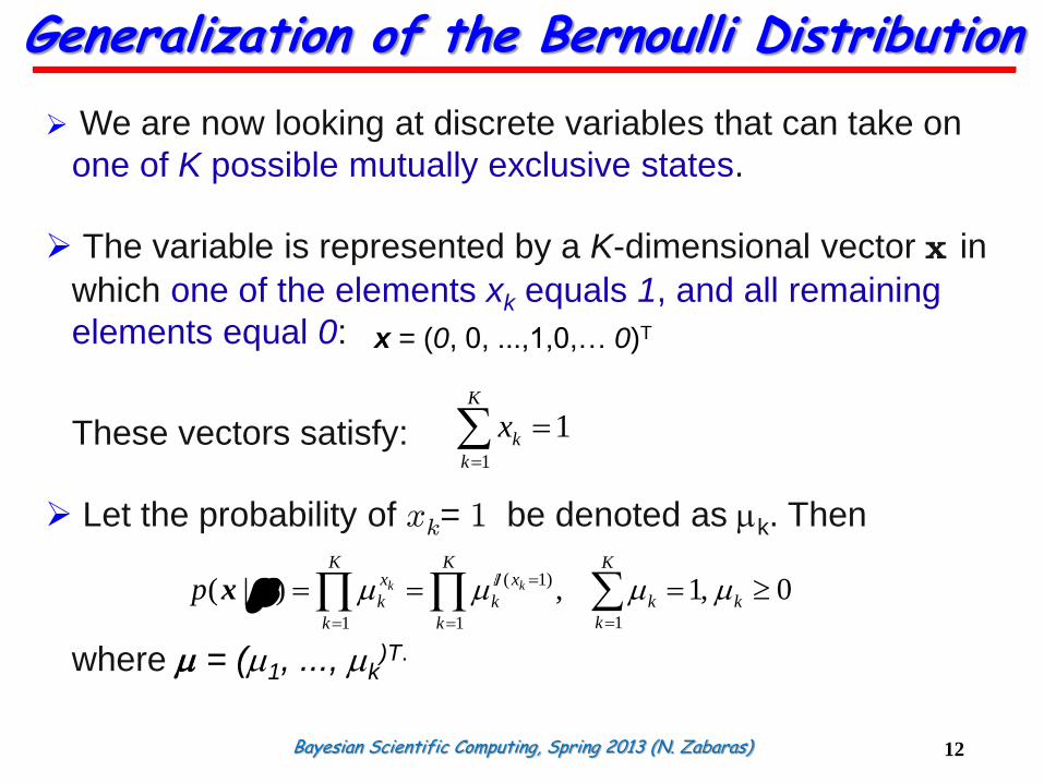
We are now looking at discrete variables that can take on

one of K possible mutually exclusive states.

The variable is represented by a K-dimensional vector x in

which one of the elements xk equals 1, and all remaining

elements equal 0:

These vectors satisfy:

Let the probability of xk = 1 be denoted as k. Then

where = (1, ..., k)T.

Generalization of the Bernoulli Distribution

12

x = (0, 0, ...,1,0,… 0)T

1

1K

k

k

x

( 1)

11 1

( | ) , 1, 0k k

K K Kx x

k k k k

kk k

p

x

Bayesian Scientific Computing, Spring 2013 (N. Zabaras)

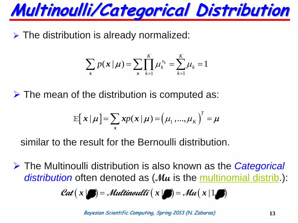
The distribution is already normalized:

The mean of the distribution is computed as:

similar to the result for the Bernoulli distribution.

The Multinoulli distribution is also known as the Categorical

distribution often denoted as (Mu is the multinomial distrib.):

Multinoulli/Categorical Distribution

13

11

( | ) 1k

K Kx

k k

kk

p

x x

x

1| ( | ) ,...,T

Kp x

x x x

| | |1, x x x Cat Multinoulli Mu

Bayesian Scientific Computing, Spring 2013 (N. Zabaras)

Let us consider a data set . The likelihood

becomes:

is the # of observations of xk=1.

mk is the sufficient statistic of the distribution.

Likelihood: Multinoulli Distribution

14

1

11 1 1 1

( | ) , :

N

nk

nk n k

N K K K Nxx m

k k k k nk

nn k k k

p where m x

D

1,..., ND x x

Bayesian Scientific Computing, Spring 2013 (N. Zabaras)

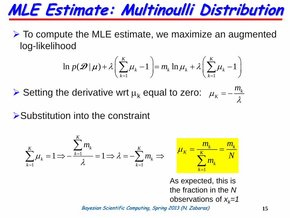
To compute the MLE estimate, we maximize an augmented

log-likelihood

Setting the derivative wrt k equal to zero:

Substitution into the constraint

MLE Estimate: Multinoulli Distribution

15

1 1

ln ( | ) 1 ln 1K K

k k k k

k k

p ml l

D

kK

m

l

1

1 1

1 1

K

kK Kk

k k

k k

m

m ll

1

k kK K

k

k

m m

Nm

As expected, this is

the fraction in the N

observations of xk=1

Bayesian Scientific Computing, Spring 2013 (N. Zabaras)

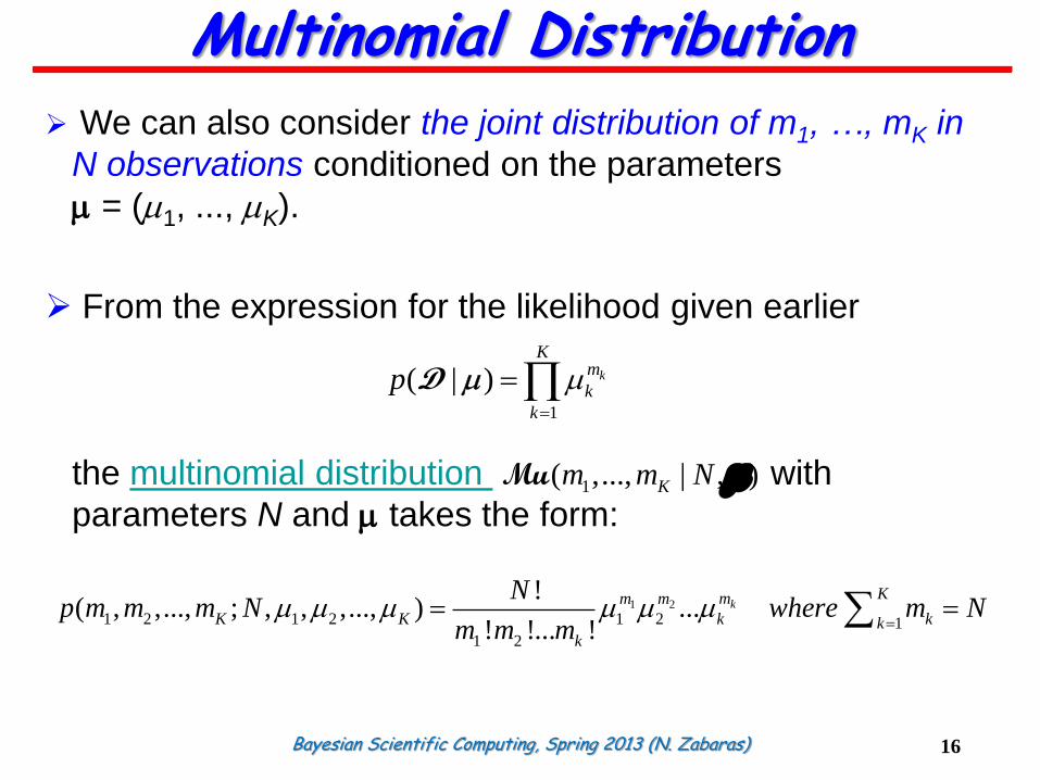
We can also consider the joint distribution of m1, …, mK in

N observations conditioned on the parameters

= (1, ..., K).

From the expression for the likelihood given earlier

the multinomial distribution with

parameters N and takes the form:

1 2

1 2 1 2 1 2 11 2

!( , ,..., ; , , ,..., ) ...

! !... !k

Kmm m

K K k kkk

Np m m m N where m N

m m m

Multinomial Distribution

16

1

( | ) k

Km

k

k

p

D

1( ,..., | , )Km m N Mu

Bayesian Scientific Computing, Spring 2013 (N. Zabaras)

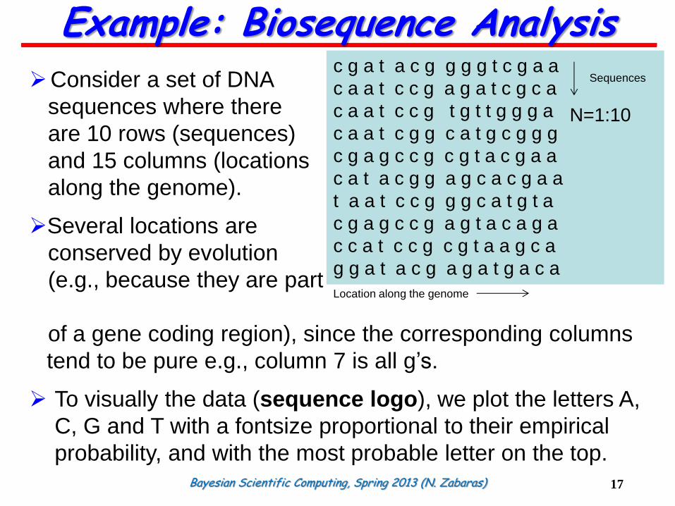
Consider a set of DNA

sequences where there

are 10 rows (sequences)

and 15 columns (locations

along the genome).

Several locations are

conserved by evolution

(e.g., because they are part

of a gene coding region), since the corresponding columns

tend to be pure e.g., column 7 is all g’s.

To visually the data (sequence logo), we plot the letters A,

C, G and T with a fontsize proportional to their empirical

probability, and with the most probable letter on the top.

Example: Biosequence Analysis

17

c g a t a c g g g g t c g a a

c a a t c c g a g a t c g c a

c a a t c c g t g t t g g g a

c a a t c g g c a t g c g g g

c g a g c c g c g t a c g a a

c a t a c g g a g c a c g a a

t a a t c c g g g c a t g t a

c g a g c c g a g t a c a g a

c c a t c c g c g t a a g c a

g g a t a c g a g a t g a c a

N=1:10

Sequences

Location along the genome

Bayesian Scientific Computing, Spring 2013 (N. Zabaras)

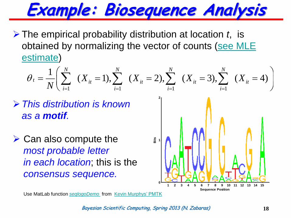
The empirical probability distribution at location t, is

obtained by normalizing the vector of counts (see MLE

estimate)

This distribution is known

as a motif.

Can also compute the

most probable letter

in each location; this is the

consensus sequence.

Use MatLab function seqlogoDemo from Kevin Murphys’ PMTK

Example: Biosequence Analysis

18

1 2 3 4 5 6 7 8 9 10 11 12 13 14 150

1

2

Sequence Position

Bit

s

1 1 1 1

1( 1), ( 2), ( 3), ( 4)

N N N N

t it it it it

i i i i

X X X XN

Bayesian Scientific Computing, Spring 2013 (N. Zabaras)

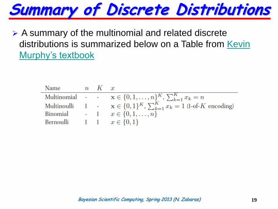
A summary of the multinomial and related discrete

distributions is summarized below on a Table from Kevin

Murphy’s textbook

Summary of Discrete Distributions

19

Bayesian Scientific Computing, Spring 2013 (N. Zabaras)

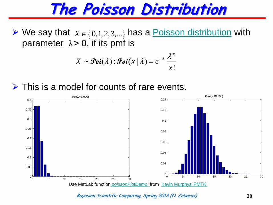
We say that has a Poisson distribution with

parameter l> 0, if its pmf is

This is a model for counts of rare events.

The Poisson Distribution

20

0,1,2,3,...X

( ) : ( | )!

x

X x ex

l ll l ~Poi Poi

0 5 10 15 20 25 300

0.02

0.04

0.06

0.08

0.1

0.12

0.14Poi(l=10.000)

0 5 10 15 20 25 300

0.05

0.1

0.15

0.2

0.25

0.3

0.35

0.4Poi(l=1.000)

Use MatLab function poissonPlotDemo from Kevin Murphys’ PMTK

Bayesian Scientific Computing, Spring 2013 (N. Zabaras)

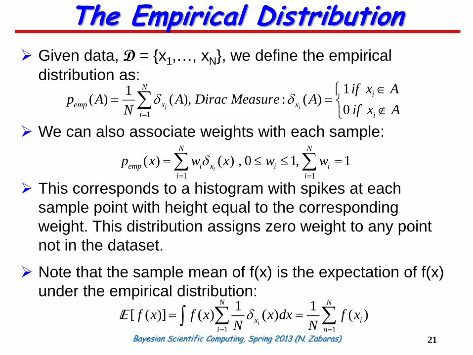
Given data, D = {x1,…, xN}, we define the empirical

distribution as:

We can also associate weights with each sample:

This corresponds to a histogram with spikes at each

sample point with height equal to the corresponding

weight. This distribution assigns zero weight to any point

not in the dataset.

Note that the sample mean of f(x) is the expectation of f(x)

under the empirical distribution:

The Empirical Distribution

21

1

11( ) ( ), : ( )

0i i

Ni

emp x x

i i

if x Ap A A Dirac Measure A

if x AN

1 1

( ) ( ) , 0 1, 1i

N N

emp i x i i

i i

p x w x w w

1 1

1 1[ ( )] ( ) ( ) ( )

i

N N

x i

i n

f x f x x dx f xN N