1

Binary Optimization via MathematicalProgramming with Equilibrium Constraints

Ganzhao Yuan, Bernard Ghanem

Abstract—Binary optimization is a central problem in mathematical optimization and its applications are abundant. To solve thisproblem, we propose a new class of continuous optimization techniques which is based on Mathematical Programming withEquilibrium Constraints (MPECs). We first reformulate the binary program as an equivalent augmented biconvex optimization problemwith a bilinear equality constraint, then we propose two penalization/regularization methods (exact penalty and alternating direction) tosolve it. The resulting algorithms seek desirable solutions to the original problem via solving a sequence of linear programming convexrelaxation subproblems. In addition, we prove that both the penalty function and augmented Lagrangian function, induced by addingthe complementarity constraint to the objectives, are exact, i.e., they have the same local and global minima with those of the originalbinary program when the penalty parameter is over some threshold. The convergence of both algorithms can be guaranteed, sincethey essentially reduce to block coordinate descent in the literature. Finally, we demonstrate the effectiveness and versatility of ourmethods on several important problems, including graph bisection, constrained image segmentation, dense subgraph discovery,modularity clustering and Markov random fields. Extensive experiments show that our methods outperform existing popular techniques,such as iterative hard thresholding, linear programming relaxation and semidefinite programming relaxation.

Index Terms—Binary Optimization, Convergence Analysis, MPECs, Exact Penalty Method, Alternating Direction Method, GraphBisection, Constrained Image Segmentation, Dense Subgraph Discovery, Modularity Clustering, Markov Random Fields.

F

1 INTRODUCTION

In this paper, we mainly focus on the following binary optimiza-tion problem:

minx

f(x), s.t. x ∈ −1, 1n, x ∈ Ω (1)

where the objective function f : Rn → R is convex (but notnecessarily smooth) on some convex set Ω, and the non-convexityof (1) is only caused by the binary constraints. In addition, weassume −1, 1n ∩ Ω 6= ∅.

The optimization in (1) describes many applications of in-terest in both computer vision and machine learning, includinggraph bisection [25], [37], image (co-)segmentation [35], [37],[54], Markov random fields [8], permutation problem [22], graphmatching [16], [59], [67], binary matrix completion [17], [31],hashing coding [42], [62], image registration [63], multimodalfeature learning [57], multi-target tracking [55], visual align-ment [56], and social network analysis (e.g. subgraphs discovery[2], [72], biclustering [1], planted k-disjoint-clique discover [4],planted clique and biclique discovery [3], community discovery[13], [29]), etc.

The binary optimization problem is difficult to solve, since it isNP-hard. One type of method to solve this problem is continuousin nature. The simple way is to relax the binary constraint withLinear Programming (LP) relaxation constraints −1 ≤ x ≤ 1and round the entries of the resulting continuous solution to thenearest integer at the end. However, not only may this solution notbe optimal, it may not even be feasible and violate some constraint.

• Ganzhao Yuan (yuanganzhao@gmail.com) is with Sun Yat-sen University(SYSU), China. Bernard Ghanem (bernard.ghanem@kaust.edu.sa) is withKing Abdullah University of Science and Technology (KAUST), SaudiArabia.

Manuscript received April 19, 2005; revised August 26, 2015.

Another type of optimization focuses on the cutting-plane andbranch-and-cut method. The cutting plane method solves the LPrelaxation and then adds linear constraints that drive the solutiontowards integers. The branch-and-cut method partially developsa binary tree and iteratively cuts out the nodes having a lowerbound that is worse than the current upper bound, while thelower bound can be found using convex relaxation, Lagrangianduality, or Lipschitz continuity. However, this class of methodends up solving all 2n convex subproblems in the worst case. Ouralgorithm aligns with the first research direction. It solves a convexLP relaxation subproblem iteratively, but it provably terminates inpolynomial iterations.

In non-convex optimization, good initialization is very im-portant to the quality of the solution. Motivated by this, severalpapers design smart initialization strategies and establish opti-mality qualification of the solutions for non-convex problems.For example, the work of [73] considers a multi-stage convexoptimization algorithm to refine the global solution by the initialconvex method; the work of [12] starts with a careful initializationobtained by a spectral method and improves this estimate bygradient descent; the work of [34] uses the top-k singular vectorsof the matrix as initialization and provides theoretical guaranteesthrough biconvex alternating minimization. The proposed methodalso uses a similar initialization strategy, as it reduces to convexLP relaxation in the first iteration.

The contributions of this paper are three-fold. (a) We refor-mulate the binary program as an equivalent augmented optimiza-tion problem with a bilinear equality constraint via a variationalcharacterization of the binary constraint. Then, we propose twopenalization/regularization methods (exact penalty and alternatingdirection) to solve it. The resulting algorithms seek desirablesolutions to the original binary program. (b) We prove that boththe penalty function and augmented Lagrangian function, inducedby adding the complementarity constraint to the objectives, are

arX

iv:1

608.

0442

5v4

[m

ath.

OC

] 6

Dec

201

7

2

TABLE 1: Existing continuous methods for binary optimization.

Method and Reference DescriptionR

elax

edA

ppro

xim

atio

n spectral relaxation [15], [54] −1,+1n ≈ x | ‖x‖22 = nlinear programming relaxation [31], [38] −1,+1n ≈ x | − 1 ≤ x ≤ 1

SDP relaxation [37], [63], [64]0,+1n ≈ x |X xxT , diag(X) = x−1,+1n ≈ x |X xxT , diag(X) = 1

doubly positive relaxation [33], [64] 0,+1n ≈ x |X xxT , diag(X) = x, x ≥ 0, X ≥ 0completely positive relaxation [10], [11] 0,+1n ≈ x |X xxT , diag(X) = x, x ≥ 0, X is CPSOCP relaxation [24], [39] −1,+1n ≈ x | 〈X− xxT ,LLT 〉 ≥ 0, diag(X) = 1, ∀ L

Equ

ival

entO

ptim

izat

ion

iterative hard thresholding [5], [72] minx ‖x− x′‖22, s.t. x ∈ −1,+1n

`0 norm reformulation [43], [70] −1,+1n ⇔ x | ‖x+ 1‖0 + ‖x− 1‖0 ≤ npiecewise separable reformulation [74] −1,+1n ⇔ x | (1+ x) (1− x) = 0`2 box non-separable reformulation [45], [51] −1,+1n ⇔ x | − 1 ≤ x ≤ 1, ‖x‖22 = n`p box non-separable reformulation [66] −1,+1n ⇔ x | − 1 ≤ x ≤ 1, ‖x‖pp = n, 0 < p <∞`∞ box separable MPEC [This paper] −1,+1n ⇔ x | x v = 1, ‖x‖∞ ≤ 1, ‖v‖∞ ≤ 1, ∀v`2 box separable MPEC [This paper] −1,+1n ⇔ x | x v = 1, ‖x‖∞ ≤ 1, ‖v‖22 ≤ n, ∀v`∞ box non-separable MPEC [This paper] −1,+1n ⇔ x | 〈x,v〉 = n, ‖x‖∞ ≤ 1, ‖v‖∞ ≤ 1, ∀v`2 box non-separable MPEC [This paper] −1,+1n ⇔ x | 〈x,v〉 = n, ‖x‖∞ ≤ 1, ‖v‖22 ≤ n, ∀v

exact, i.e., the set of their globally optimal solutions coincide withthat of (1) when the penalty parameter is over some threshold.Thus, the convergence of both algorithms can be guaranteed sincethey reduce to block coordinate descent in the literature [7], [60].To our best knowledge, this is the first attempt to solve generalnon-smooth binary program with guaranteed convergence. (c) Weprovide numerical comparisons with state-of-the-art techniques,such as iterative hard thresholding [72], linear programming re-laxation [38], [39] and semidefinite programming relaxation [63]on a variety of concrete computer vision and machine learningproblems. Extensive experiments have demonstrated the effective-ness of our proposed methods. A preliminary version of this paperappeared in AAAI 2017 [71].

This paper is organized as follows. Section 2 provides a briefdescription of the related work. Section 3 presents our MPEC-based optimization framework. Section 4 discusses some featuresof our methods. Section 5 summarizes the experimental results.Finally, Section 6 concludes this paper. Throughout this paper,we use lowercase and uppercase boldfaced letters to denote realvectors and matrices respectively. The Euclidean inner productbetween x and y is denoted by 〈x,y〉 or xTy. We use In todenote an identity matrix of size n, where sometimes the subscriptis dropped when n is known from the context. X 0 meansthat matrix X is positive semi-definite. Finally, sign is a signumfunction with sign(0) = ±1.

2 RELATED WORK

This paper proposes a new continuous method for binary opti-mization. We briefly review existing related work in this researchdirection in the literature (see Table 1).

There are generally two types of methods in the literature.One is the relaxed approximation method. Spectral relaxation [15],[41], [49], [54] replaces the binary constraint with a sphericalone and solves the problem using eigen decomposition. Despiteits computational merits, it is difficult to generalize to handlelinear or nonlinear constraints. Linear programming relaxation

[38], [39] transforms the NP-hard optimization problem intoa convex box-constrained optimization problem, which can besolved by well-established optimization methods and software.Semi-Definite Programming (SDP) relaxation [33] uses a liftingtechnique X = xxT and relaxes to a convex conic X xxT 1 tohandle the binary constraint. Combining this with a unit-ball ran-domized rounding algorithm, the work of [25] proves that at least afactor of 87.8% to the global optimal solution can be achieved forthe graph bisection problem. Since the original paper of [25], SDPhas been applied to develop numerous approximation algorithmsfor NP-hard problems. As more constraints lead to tighter boundsfor the objective, doubly positive relaxation considers constrainingboth the eigenvalues and the elements of the SDP solution tobe nonnegative, leading to better solutions than canonical SDPmethods. In addition, Completely Positive (CP) relaxation [10],[11] further constrains the entries of the factorization of thesolution X = LLT to be nonnegative L ≥ 0. It can be solvedby tackling its associated dual co-positive program, which isrelated to the study of indefinite optimization and sum-of-squaresoptimization in the literature. Second-Order Cone Programming(SOCP) relaxes the SDP conic into the nonnegative orthant [39]using the fact that 〈X − xxT ,LLT 〉 ≥ 0, ∀ L, resulting intighter bound than the LP method, but looser than that of theSDP method. Therefore it can be viewed as a balance betweenefficiency and efficacy.

Another type of methods for binary optimization relates toequivalent optimization. The iterative hard thresholding methoddirectly handles the non-convex constraint via projection and ithas been widely used due to its simplicity and efficiency [72].However, this method is often observed to obtain sub-optimalaccuracy and it is not directly applicable, when the objectiveis non-smooth. A piecewise separable reformulation has beenconsidered in [74], which can exploit existing smooth optimizationtechniques. Binary optimization can be reformulated as an `0 norm

1. Using Schur complement lemma, one can rewrite X xxT as(X xxT 1

) 0.

3

semi-continuous optimization problem2. Thus, existing `0 normsparsity constrained optimization techniques such as quadraticpenalty decomposition method [43] and multi-stage convex op-timization method [70], [73] can be applied. A continuous `2 boxnon-separable reformulation3 has been used in the literature [36],[50], [51]. A second-order interior point method [18], [45] hasbeen developed to solve the continuous reformulation optimiza-tion problem. A continuous `p box non-separable reformulationhas recently been used in [66], where an interesting geometricillustration of `p-box intersection has been shown4. In addition,they infuse this equivalence into the optimization framework ofAlternating Direction Method of Multipliers (ADMM). However,their guarantee of convergence is weak. In this paper, to tacklethe binary optimization problem, we propose a new frameworkthat is based on Mathematical Programming with EquilibriumConstraints (MPECs) (refer to the proposed MPEC reformulationsin Table 1). Our resulting algorithms are theoretically convergentand empirically effective.

Mathematical programs with equilibrium constraints5 are op-timization problems where the constraints include complementar-ities or variational inequalities. They are difficult to deal with be-cause their feasible region may not necessarily be convex or evenconnected. Motivated by recent development of MPECs for non-convex optimization [6], [44], [68], [69], [70], we consider con-tinuous MPEC reformulations of the binary optimization problem.Since our preliminary experimental results show that `2 box non-separable MPEC in Table 1 often presents the best performance interms of accuracy, we only focus on this specific formulation inour forthcoming algorithm design and numerical experiments. Forfuture references, other possible separable/non-separable6 MPECreformulations are presented here. Their mathematical derivationand mathematical treatment are similar.

3 PROPOSED OPTIMIZATION ALGORITHMS

This section presents our MPEC-based optimization algorithms.We first propose an equivalent reformulation of binary optimiza-tion program, and then we consider two algorithms (exact penaltymethod and alternating direction method) to solve it.

3.1 Equivalent Reformulation

First of all, we present a variational reformulation of the binaryconstraint. The proofs for other reformulations of binary con-straints can be found in Appendix A.

Lemma 1. `2 box non-separable MPEC. We define Θ ,(x,v) | xTv = n, ‖x‖∞ ≤ 1, ‖v‖22 ≤ n. Assume that

2. One can rewrite the `0 norm constraint ‖x + 1‖0 + ‖x− 1‖0 ≤ n in acompact matrix form ‖Ax−b‖0 ≤ n with A = [In | In]T ∈ R2n×n, b =[1T | − 1T ]T ∈ R2n.

3. They replace x ∈ 0, 1n with 0 ≤ x ≤ 1, xT (1−x) = 0. We extendthis strategy to replace −1,+1n with−1 ≤ x ≤ 1, (1+x)T (1−x) = 0which reduces to ‖x‖∞ ≤ 1, ‖x‖22 = n. Appendix 6 provides a simple proof.

4. We adapt their formulation to our −1,+1 formulation.5. In fact, we focus on mathematical programs with complementarity con-

straints (MPCC), a subclass of MPECs where the original discrete optimizationproblem can be formulated as a complementarity problem and therefore as anonlinear program. Here we use the term MPECs for the purpose of generalityand historic conventions.

6. Note that separable MPEC has n complementarity constraints and non-separable MPEC has one complementarity constraint. The terms separable andnon-separable are related to whether the constraints can be decomposed toindependent components.

(x,v) ∈ Θ, then we have x ∈ −1,+1n, v ∈ −1,+1n, andx = v.

Proof. (i) Firstly, we prove that x ∈ −1,+1n. Using thedefinition of Θ and the Cauchy-Schwarz Inequality, we have: n =xTv ≤ ‖x‖2‖v‖2 ≤ ‖x‖2

√n =√nxTx ≤

√n‖x‖1‖x‖∞ ≤√

n‖x‖1. Thus, we obtain ‖x‖1 ≥ n. We define z = |x|.Combining ‖x‖∞ ≤ 1, we have the following constraint setsfor z:

∑i zi ≥ n, 0 ≤ z ≤ 1. Therefore, we have z = 1

and it holds that x ∈ −1,+1n. (ii) Secondly, we prove thatv ∈ −1,+1n. We have:

n = xTv ≤ ‖x‖∞‖v‖1 ≤ ‖v‖1 = |v|T1 ≤ ‖v‖2‖1‖2 (2)

Thus, we obtain ‖v‖2 ≥√n. Combining ‖v‖22 ≤ n, we have

‖v‖2 =√n and ‖v‖2‖1‖2 = n. By the Squeeze Theorem,

all the equalities in (2) hold automatically. Using the equalitycondition for Cauchy-Schwarz Inequality, we have |v| = 1 and itholds that v ∈ −1,+1n.

(iii) Finally, since x ∈ −1,+1n, v ∈ −1,+1n, and〈x,v〉 = n, we obtain x = v.

Using Lemma 1, we can rewrite (1) in an equivalent form asfollows.

min−1≤x≤1, ‖v‖22≤n

f(x), s.t. xTv = n, x ∈ Ω (3)

We remark that xTv = n is called complementarity (or equi-librium) constraint in the literature [44], [52], [58] and it alwaysholds that xTv ≤ ‖x‖∞‖v‖1 ≤

√n‖v‖2 ≤ n for any feasible

x and v.

3.2 Exact Penalty MethodWe now present our exact penalty method for solving the opti-mization problem in (3). It is worthwhile to point out that thereare many studies on exact penalty for MPECs (refer to [32], [44],[52], [70] for examples), but they do not afford the exactness ofour penalty problem. In an exact penalty method, we penalize thecomplementary error directly by a penalty function. The resultingobjective J : Rn × Rm → R is defined in (4), where ρ isthe penalty parameter that is iteratively increased to enforce thebilinear constraint.

Jρ(x,v) = f(x) + ρ(n− xTv)

s.t. − 1 ≤ x ≤ 1, ‖v‖22 ≤ n, x ∈ Ω(4)

In each iteration, we minimize over x and v alternatingly [7], [60],while fixing the parameter ρ. We summarize our exact penaltymethod in Algorithm 1. The parameter T is the number of inneriterations for solving the biconvex problem and the parameter Lis the Lipschitz constant of the objective function f(·). We makethe following observations about the algorithm.(a) Initialization. We initialize v0 to 0. This is for the sake offinding a reasonable local minimum in the first iteration, as itreduces to LP convex relaxation [38] for the binary optimizationproblem.(b) Exact property. One remarkable feature of our method isthe boundedness of the penalty parameter ρ (see Theorem 1).Therefore, we terminate the optimization when the threshold isreached (see (7) in Algorithm 1). This distinguishes it from thequadratic penalty method [43], where the penalty may becomearbitrarily large for non-convex problems.

4

Algorithm 1 MPEC-EPM: An Exact Penalty Method for SolvingMPEC Problem (3)(S.0) Set t = 0, x0 = v0 = 0, ρ > 0, σ > 1.(S.1) Solve the following x-subproblem [primal step]:

xt+1 = arg minx

J (x,vt), s.t. x ∈ [−1,+1]n ∩ Ω (5)

(S.2) Solve the following v-subproblem [dual step]:

vt+1 = arg minv

J (xt+1,v), s.t. ‖v‖22 ≤ n (6)

(S.3) Update the penalty in every T iterations:

ρ⇐ min(2L, ρ× σ) (7)

(S.4) Set t := t+ 1 and then go to Step (S.1)

(c) v-Subproblem. Variable v in (6) is updated by solving thefollowing convex problem:

vt+1 = arg min 〈v,−xt+1〉, s.t. ‖v‖22 ≤ n (8)

When xt+1 = 0, any feasible solution is also an optimal solution;when xt+1 6= 0, the optimal solution will be achieved in theboundary with ‖v‖22 = n and (8) is equivalent to solving:min‖v‖22=n

12‖v‖

22 − 〈v,xt+1〉. Thus, we have the following

optimal solution for v:

vt+1 =

√n · xt+1/‖xt+1‖2, xt+1 6= 0;

any v with ‖v‖22 ≤ n, otherwise. (9)

(d) x-Subproblem. Variable x in (5) is updated by solving boxconstrained convex problem which has no closed-form solution.However, it can be solved using Nesterov’s proximal gradientmethod [46] or classical/linearized ADM [28].

Theoretical Analysis. In the following, we present sometheoretical analysis of our exact penalty method. The followinglemma is very crucial and useful in our proofs.

Lemma 2. We define:

h∗ ,

(min

x∈Rn, −1≤x≤1, sign(x)6=xh(x)

)with h(x) ,

n−√n‖x‖2

‖sign(x)− x‖2

(10)

It holds that h∗ ≥ 1/2.

Proof. We define B and N as the index set of the binary and non-binary variable for any x ∈ Rn, respectively. Therefore, we have|xi| = 1, ∀i ∈ B and |xj | 6= 1, ∀j ∈ N . Moreover, we defines , |N | and we have |B| = n− s. We can rewrite h(x) as

h(x) =n−√n√‖xB‖22 + ‖xN‖22√

‖sign(xB)− xB‖22 + ‖sign(xN )− xN‖22

=n−√n√|B|+ ‖xN‖22√

0 + ‖sign(xN )− xN‖22We have the following problem which is equivalent to (10)

minz∈Rs

h′(z) =n−√n√|B|+ ‖z‖22√

‖sign(z)− z‖22s.t. −1 ≤ z ≤ 1, |z|i 6= 1,∀i

(11)

We notice that the function h′(z) has the property that h′(z) =h′(−z) = h′(Pz) for any perturbation matrix P with P ∈

0, 1s×s, P1 = 1, 1P = 1. Therefore, the optimal solutionz∗ for problem (11) will be achieved with |z∗1| = |z∗2| =, ...,=|z∗s| = δ for some unknown constant δ with 0 < δ < 1.Therefore, we have the following optimization problem which isequivalent to (10) and (11)

mins,δ

J(s, δ) ,n−√n√n− s+ sδ2√

s(1− δ)2, s.t. s ∈ 1, 2., , , .n (12)

Since J(s, δ) is an increasing function for any δ ∈ (0, 1), theoptimal solution s∗ for (12) with be achieved with s∗ = 1.Therefore, we derive the following inequalities:

h∗ ≥ n−√n√

(n− 1) + δ2√(1− δ)2

, p(δ) (13)

In what follows, we prove that p(δ) > 1/2 on 0 < δ < 1for any n. First of all, it is not hard to validate that p(δ) is adecreasing function on 0 < δ < 1 for any n. We now considerthe two limit points for p(δ) in (13). (i) We have limδ→0+ p(δ) =n −√n2 − n > 1/2 due to the following inequalities: 1/4 >

0 ⇒ n2 − n + 1/4 > n2 − n ⇒ (n − 1/2)2 > n2 − n ⇒(n − 1/2) >

√n2 − n ⇒ n −

√n2 − n > 1/2. (ii) More-

over, we have limδ→1− p(δ) = limδ→1−n−√n√

(n−1)+δ2√(1−δ)2

=

limδ→1−n−√n2−n+δ2n1−δ > 1/2. Hereby we finish the proof of

this lemma.

The following lemma is useful in establishing the exactnessproperty of the penalty function in Algorithm 1.

Lemma 3. Consider the following optimization problem:

(x∗ρ,v∗ρ) = arg min

−1≤x≤1, ‖v‖22≤n, x∈ΩJρ(x,v). (14)

Assume that f(·) is a L-Lipschitz continuous convex function on−1 ≤ x ≤ 1. When ρ > 2L, 〈x∗ρ,v∗ρ〉 = n will be achieved forany local optimal solution of (14).

Proof. To finish the proof of this lemma, we consider two cases:x = sign(x) and x 6= sign(x). For the first case, x = sign(x)implies that the solution is binary, any ρ guarantees that the com-plimentary constraint is satisfied. The conclusion of this lemmaclearly holds. Now we consider the case that x 6= sign(x).

First of all, we focus on the v-subproblem in the optimizationproblem in (14).

v∗ρ = arg minv− xTv, s.t. ‖v‖22 ≤ n (15)

Assume that x∗ρ 6= 0, we have v∗ρ =√n · x∗ρ/‖x∗ρ‖2. Then the

biconvex optimization problem reduces to the following:

x∗ρ = arg min−1≤x≤1

p(x) , f(x) + ρ(n−√n‖x‖2) (16)

For any x∗ρ ∈ Ω, we derive the following inequalities:

0.5ρ‖sign(x∗ρ)− x∗ρ‖2≤ ρ(n−

√n‖x∗ρ‖2)

= [ρ(n−√n‖x∗ρ‖2) + f(x∗ρ)]− f(x∗ρ)

≤ [ρ(n−√n‖sign(x∗ρ)‖2) + f(sign(x∗ρ))]f(x∗ρ)

= f(sign(x∗ρ))− f(x∗ρ)

= L‖sign(x∗ρ)− x∗ρ‖2 (17)

where the first step uses Lemma 2 that ‖sign(x) − x‖2 ≤2(n −

√n‖x‖2) for any x in ‖x‖∞ ≤ 1; the third steps uses

5

the optimality of x∗ρ in (16) that p(x∗ρ) ≤ p(y) for any y with−1 ≤ y ≤ 1, y ∈ Ω; the fourth step uses the fact thatsign(xρ) ∈ −1,+1n and

√n‖sign(xρ)‖2 = n; the last step

uses the Lipschitz continuity of f(·).From (17), we have ‖x∗ρ − sign(x∗ρ)‖2 · (ρ − 2L) ≤ 0.

Since ρ − 2L > 0, we conclude that it always holds that‖x∗ρ − sign(x∗ρ)‖2 = 0. Thus, x∗ρ ∈ −1,+1n. Finally, wehave x∗ρ =

√n · x∗ρ/‖x∗ρ‖2 = v∗ρ and 〈x∗ρ,v∗ρ〉 = n.

The following theorem shows that when the penalty parameterρ is larger than some threshold, the biconvex objective functionin (4) is equivalent to the original constrained MPEC problemin (3). This essentially implies the theoretical convergence ofthe algorithm since it reduces to block coordinate descent in theliterature7.

Theorem 1. Exactness of the Penalty Function. Assume thatf(·) is a L-Lipschitz continuous convex function on−1 ≤ x ≤ 1.When ρ > 2L, the biconvex optimization in (4) has the same localand global minima with the original problem in (3).

Proof. We let x∗ be any global minimizer of (3) and (x∗ρ,v∗ρ) be

any global minimizer of (4) for some ρ > 2L.(i) We now prove that x∗ is also a global minimizer of (4). For

any feasible x and v that ‖x‖∞ ≤ 1, ‖v‖22 ≤ n, we derive thefollowing inequalities:

J (x,v, ρ)

≥ min‖x‖∞≤1, ‖v‖22≤n, x∈Ω

f(x) + ρ(n− xTv)

= min‖x‖∞≤1, ‖v‖22≤n, x∈Ω

f(x), s.t. xTv = n

= f(x∗) + ρ(n− x∗Tv∗)

= J (x∗,v∗, ρ)

where the first equality holds due to the fact that the constraintxTv = n is satisfied at the local optimal solution when ρ > 2L(see Lemma 3). Therefore, we conclude that any optimal solutionof (3) is also an optimal solution of (4).

(ii) We now prove that x∗ρ is also a global minimizer of (3).For any feasible x and v that ‖x‖∞ ≤ 1, ‖v‖22 ≤ n, xTv =n, x ∈ Ω, we naturally have the following inequalities:

f(x∗ρ)− f(x)

= f(x∗ρ) + ρ(n− x∗Tρ v∗ρ)− f(x)− ρ(n− xTv)

= Jρ(x∗ρ,v∗ρ)− Jρ(x,v)

≤ 0

where the first equality uses Lemma 3. Therefore, we concludethat any optimal solution of (4) is also an optimal solution of (3).

Finally, we conclude that when ρ > 2L, the biconvex opti-mization in (4) has the same local and global minima with theoriginal problem in (3).

The following the theorem characterizes the convergence rateand asymptotic monotone property the algorithm.

7. Specifically, using Tseng’s convergence results of block coordinate de-scent for non-differentiable minimization [60], one can guarantee that everyclustering point of Algorithm 2 is also a stationary point. In addition, strongerconvergence results [7], [70] can be obtained by combining a proximal strategyand Kurdyka-Łojasiewicz inequality assumption on J (·).

Theorem 2. Convergence Rate and Asymptotic Monotone Prop-erty of Algorithm 1. Assume that f(·) is a L-Lipschitz continuousconvex function on−1 ≤ x ≤ 1. Algorithm 1 will converge to thefirst-order KKT point in at most d(ln(L

√2n) − ln(ερ0))/ lnσe

outer iterations8 with the accuracy at least n − xTv ≤ ε.Moreover, after 〈x,v〉 = n is obtained, the sequence of f(xt)generated by Algorithm 1 is monotonically non-increasing.

Proof. We denote s and t as the outer iterations counter and inneriteration counter in Algorithm 1, respectively.

(i) we now prove the convergence rate of Algorithm 1. Assumethat Algorithm 1 takes s outer iterations to converge. We denotef ′(x) as the sub-gradient of f(·) in x. According the the x-subproblem in (16), if x∗ solves (16), then we have the followingvariational inequality [28]:

∀x ∈ [−1,+1]n ∩ Ω, 〈x− x∗, f ′(x∗)〉+

ρ(n−√n‖x‖2)− ρ(n−

√n‖x∗‖2) ≥ 0

Letting x be any feasible solution that x ∈ −1,+1n ∩ Ω, wehave the following inequalities:

(n−√n‖x∗‖2)

≤ (n−√n‖x‖2) + 1

ρ 〈x− x∗, f ′(x∗)〉≤ 1

ρ‖x− x∗‖2 · ‖f ′(x∗)‖2≤ L

√2n/ρ (18)

where the second inequality is due to the Cauchy-Schwarz In-equality, the third inequality is due to the fact that ‖x − y‖2 ≤√

2n, ∀ − 1 ≤ x ,y ≤ 1 and the Lipschitz continuity of f(·)that ‖f ′(x∗)‖2 ≤ L.

The inequality in (18) implies that when ρs ≥ L√

2n/ε,Algorithm 1 achieves accuracy at least n−

√n‖x‖2 ≤ ε. Noticing

that ρs = σsρ0, we have that ε accuracy will be achieved when

σsρ0 ≥ L√

2n

ε

⇒ σs ≥ L√

2n

ερ0

⇒ s ≥ (ln(L√

2n)− ln(ερ0))/ lnσ

(ii) we now prove the asymptotic monotone property of Algo-rithm 1. We naturally derive the following inequalities:

f(xt+1)− f(xt)

≤ ρ(n− 〈xt,vt〉)− ρ(n− 〈xt+1,vt〉)= ρ

(〈xt+1,vt〉 − 〈xt,vt〉

)≤ ρ

(〈xt+1,vt+1〉 − 〈xt,vt〉

)= 0

where the first step uses the fact that f(xt+1) + ρ(n −〈xt+1,vt〉) ≤ f(xt) + ρ(n − 〈xt,vt〉) holds due to xt+1

is the optimal solution of (5); the third step uses the fact−〈xt+1,vt+1〉 ≤ −〈xt+1,vt〉 holds due to vt+1 is the op-timal solution of (6); the last step uses 〈x,v〉 = n. Notethat the equality 〈x,v〉 = n together with the feasible set−1 ≤ x ≤ 1, ‖v‖22 ≤ n also implies that x ∈ −1,+1n.

We have a few remarks on the theorems above. We assume thatthe objective function is L-Lipschitz continuous. However, such

8. Every time we increase ρ, we call it one outer iteration.

6

Algorithm 2 MPEC-ADM: An Alternating Direction Methodfor Solving MPEC Problem (3)

(S.0) Set t = 0, x0 = v0 = 0, ρ0 = 0, α > 0, σ > 1.(S.1) Solve the following x-subproblem [primal step]:

xt+1 = arg minx

L(x,vt, ρt), s.t. x ∈ [−1,+1]n ∩ Ω (19)

(S.2) Solve the following v-subproblem [dual step]:

vt+1 = arg minv

L(xt+1,v, ρt) s.t. ‖v‖22 ≤ n (20)

(S.3) Update the Lagrange multiplier:

ρt+1 = ρt + α(n− 〈xt+1,vt+1〉) (21)

(S.4) Update the penalty in every T iterations (if necessary):

α⇐ α× σ (22)

(S.5) Set t := t+ 1 and then go to Step (S.1).

hypothesis is not strict. Because the solution x is defined on thecompact set, the Lipschitz constant can always be computed forany continuous objective (e.g. norm function, min/max envelopfunction). In fact, it is equivalent to say that the (sub-) gradientof the objective is bounded by L9. Although exact penalty methodhas been study in the literature [19], [20], [27], their results cannotdirectly apply here. The theoretical bound 2L (on the penaltyparameter ρ) heavily depends on the specific structure of the op-timization problem. Moreover, we also establish the convergencerate and asymptotic monotone property of our algorithm.

3.3 Alternating Direction Method

This section presents an alternating direction method (of multipli-ers) (ADM or ADMM) for solving (3). This is mainly motivatedby the recent popularity of ADM in the optimization literature[28], [64], [68], [69].

We first form the augmented Lagrangian L : Rn × Rm ×Rm → R in (23) as follows:

L(x,v, ρ) , f(x) + ρ(n− xTv) +α

2(n− xTv)2

s.t. − 1 ≤ x ≤ 1, ‖v‖22 ≤ n, x ∈ Ω(23)

where ρ is the Lagrange multiplier associated with the comple-mentarity constraint n − 〈x,v〉 = 0, and α > 0 is the penaltyparameter. Interestingly, we find that the augmented Lagrangianfunction can be viewed as adding an elastic net regularization [75]on the complementarity error. We detail the ADM iteration stepsfor (23) in Algorithm 2, which has the following properties.(a) Initialization. We set v0 = 0 and ρ0 = 0. This finds areasonable local minimum in the first iteration, as it reduces to LPrelaxation for the x-subproblem.(b) Monotone property. For any feasible solution x and v in(23), it holds that n − xTv ≥ 0. Using the fact that αt > 0 anddue to the ρt update rule, ρt is monotone increasing.

9. For example, for the quadratic function f(x) = 0.5xTAx + xTb withA ∈ Rn×n and b ∈ Rn, the Lipschitz constant is bounded by L ≤ ‖Ax +b‖ ≤ ‖A‖‖x‖ + ‖b‖ ≤ ‖A‖

√n + ‖b‖; for the `1 regression function

f(x) = ‖Ax − b‖1 with A ∈ Rm×n and b ∈ Rm, the Lipschitz constantis bounded by L ≤ ‖AT ∂|Ax− b|‖ ≤ ‖AT ‖

√m.

(c) v-Subproblem. Variable v in (20) is updated by solving thefollowing problem:

vt+1 = arg minv

1

2vTaaTv + 〈v,b〉, s.t. ‖v‖2 ≤

√n

where a , xt+1/√α and b , −(ρ+ αn) · xt+1. This problem

is also known as constrained eigenvalue problem in the literature[23], which has efficient solution. Since the quadratic matrix isof rank one, this problem has nearly closed-form solution (pleaserefer to Appendix B for detailed discussions).(d) x-Subproblem. Variable x in (23) is updated by solving a boxconstrained optimization problem. Similar to (5), it can be solvedusing Nesterov’s proximal gradient method or classical/linearizedADM.

Theoretical Analysis. In the following, we present sometheoretical analysis of our alternating direction method. The proofsof theoretical convergence are similar to our previous analysisfor the exact penalty method. The following lemma is usefulin building the exactness property of the augmented Lagrangianfunction in Algorithm 2.

Lemma 4. Consider the following optimization problem:

(x∗ρ,v∗ρ) = arg min

−1≤x≤1,‖v‖22≤n, x∈ΩL(x,v, ρ). (24)

Assume that f(·) is a L-Lipschitz continuous convex function on−1 ≤ x ≤ 1. When ρ > 2L, 〈x∗ρ,v∗ρ〉 = n will be achieved forany local optimal solution of (24).

Proof. The proof of this theorem is based on Lemma 3. Weobserve that n − xTv = 0 ⇔ (n − xTv)2 = 0. We defineh(x) , f(x) + α

2 (n − xTv)2 and denote Lh as the Lipschtzconstant of h(·). We replace f(·) with h(·) in Lemma 3 andconclude that when ρ > 2Lg , we have n − xTv = 0. Thus,the term α

2 (n− xTv)2 in h(x) reduces to zero and Lh = L. Weconclude that when ρ > 2L, 〈x∗ρ,v∗ρ〉 = n will be achieved forany local optimal solution.

Our MPEC-ADM has excellent convergence property. Thefollowing theorem shows that when the multiplier ρ is largerthan some threshold, the biconvex objective function in (23) isequivalent to the original constrained MPEC problem in (3).

Theorem 3. Exactness of the augmented Lagrangian Function.Assume that f(·) is a L-Lipschitz continuous convex function on−1 ≤ x ≤ 1. When ρ > 2L, the biconvex optimization problemminx, v L(x,v, ρ), s.t. − 1 ≤ x ≤ 1, ‖v‖22 ≤ n, x ∈ Ωin (23) has the same local and global minima with the originalproblem in (3).

Proof. The proof of this theorem is similar to Theorem 1. We letx∗ be any global minimizer of (3) and (x∗ρ,v

∗ρ) be any global

minimizer of (4) for some ρ > 2L.(i) We now prove that x∗ is also a global minimizer of (4). For

any feasible x and v that ‖x‖∞ ≤ 1, ‖v‖22 ≤ n, x ∈ Ω, wederive the following inequalities:

L(x,v, ρ)

≥ min‖x‖∞≤1, ‖v‖2≤n

f(x) + ρ(n− xTv) +α

2(n− xTv)2

= min‖x‖∞≤1, ‖v‖2≤n

f(x), s.t. xTv = n

= f(x∗) + ρ(n− x∗Tv∗) +α

2(n− x∗Tv∗)2

= L(x∗,v∗, ρ)

7

where the first equality holds due to the fact that the constraintxTv = n is satisfied at the local optimal solution when ρ > 2L(see Lemma 3). Therefore, we conclude that any optimal solutionof (3) is also an optimal solution of (4).

(ii) We now prove that x∗ρ is also a global minimizer of (3).For any feasible x and v that ‖x‖∞ ≤ 1, ‖v‖22 ≤ n, xTv =n, x ∈ Ω, we naturally have the following inequalities:

f(x∗ρ)− f(x)

= f(x∗ρ) + ρ(n− x∗Tρ v∗ρ) +α

2(n− x∗Tρ v∗ρ)

2

−f(x)− ρ(n− xTv)− α

2(n− xTv)2

= L(x∗ρ,v∗ρ, ρ)− L(x,v, ρ)

≤ 0

Therefore, we conclude that any optimal solution of (4) is also anoptimal solution of (3).

Finally, we conclude that when ρ > 2L, the biconvex opti-mization in (4) has the same local and global minima with theoriginal problem in (3).

We have some remarks on the theorem above. We use the sameassumption as in the exact penalty method. Although alternatingdirection method has been used in the literature [40], [66], theirconvergence results are much weaker than ours. The main nov-elties of our method is the self-penalized feature owning to theboundedness and monotone property of multiplier.

4 DISCUSSIONS

This section discusses the comparisons of MPEC-EPM andMPEC-ADM, the merits of our methods, and the extensions tozero-one constraint and orthogonality constraint.

MPEC-EPM vs. MPEC-ADM. The proposed MPEC-EPMand MPEC-ADM have their own advantages. (a) MPEC-EPMis more simple and elegant and it can directly use existingLP relaxation optimization solver. (b) MPEC-EPM may be lessadaptive since the penalty parameter ρ is monolithically increaseduntil a threshold is achieved. In comparison, MPEC-ADM is moreadaptive, since a constant penalty also guarantees monotonicallynon-decreasing multipliers and convergence.

Merits of our methods. There are several merits behind ourMPEC-based penalization/regularization methods. (a) They ex-hibit strong convergence guarantees since they essentially reduceto block coordinate descent in the literature [7], [60]. (b) They seekdesirable solutions since the LP convex relaxation methods in thefirst iteration provide good initializations. (c) They are efficientsince they are amenable to the use of existing convex methodsto solve the sub-problems. (d) They have a monotone/greedyproperty due to the complimentary constraints brought on byMPECs. We penalize the complimentary error and ensure that theerror is decreasing in every iteration, leading to binary solutions.

Extensions to Zero-One Constraint and OrthogonalityConstraint. For convenience, we define ∆ = 0, 1n andO = X ∈ Rn×r | XTX = Ir (n ≥ r). Noticing thaty = (x + 1)/2 ∈ 0, 1n, we can extend `∞ box non-separableMPEC10 and `2 box non-separable MPEC11 to handle zero-onebinary optimization. Moreover, observing that binary constraint

10. ∆⇔ x | 0 ≤ x ≤ 1, 0 ≤ v ≤ 1, 〈2x− 1, 2v − 1〉 = n, ∀v11. ∆⇔ x | 0 ≤ x ≤ 1, ‖2v− 1‖22 ≤ n, 〈2x−1, 2v−1〉 = n, ∀v

x ∈ −1,+1n ⇔ |x| = 1 is analogous to orthogonalityconstraint since X ∈ O ⇔ σ(X) = 1, we can extend our `∞box non-separable MPEC12 and `2 box non-separable MPEC13 tothe optimization problem with orthogonality constraint [14], [65].

5 EXPERIMENTAL VALIDATION

In this section, we demonstrate the effectiveness of our algo-rithms (MPEC-EPM and MPEC-ADM) on 5 binary optimizationtasks, namely graph bisection, constrained image segmentation,dense subgraph discovery, modularity clustering and Markovrandom fields. All codes are implemented in MATLAB using a3.20GHz CPU and 8GB RAM. For the purpose of reproducibil-ity, we provide our MATLAB code at: http://isee.sysu.edu.cn/∼yuanganzhao/.

5.1 Graph BisectionGraph bisection aims at separating the vertices of a weightedundirected graph into two disjoint sets with minimal cut edgeswith equal size. Mathematically, it can be formulated as thefollowing optimization problem [37], [63]:

minx∈−1,+1n

xTLx, s.t. xT1 = 0

where L = D−W ∈ Rn×n is the Laplacian matrix, W ∈ Rn×nis the affinity matrix and D = diag(W1) ∈ Rn×n is the degreematrix.

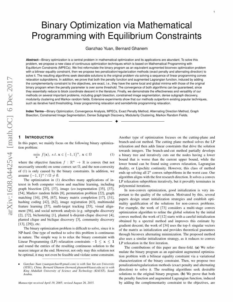
Compared Methods. We compare MPEC-EPM and MPEC-ADM against 5 methods on the ‘4gauss’ data set (see Figure 1). (i)LP relaxation simply relaxes the binary constraint to−1 ≤ x ≤ 1and solves the following problem:

LP : minx

xTLx, s.t. xT1 = 0, − 1 ≤ x ≤ 1

(ii) Ratio Cut (RCUT) and Normalize Cut (NCUT) relax thebinary constraint to ‖x‖22 = n and solve the following problems[15], [54]:

RCut : minx

xTLx, s.t. 〈x,1〉 = 0, ‖x‖22 = n

NCut : minx

xT Lx, s.t. 〈x,D1/21〉 = 0, ‖x‖22 = n

where L = D−1/2LD−1/2. The optimal solution of RCut (orNCut) is the second smallest eigenvectors of L (or L), seee.g. [37], [63]. (iv) SDP relaxation solves the following convexoptimization problem 14:

SDP : minX〈L,X〉, s.t. diag(X) = 1, 〈X,11T 〉 = 0

Finally, we also compare with L2box-ADMM [66] which appliesADMM directly to the `2 box non-separable reformulation:

minx

xTLx, s.t. xT1 = 0, − 1 ≤ x ≤ 1, ‖x‖22 = n.

We remark that it is a splitting method that introduces auxiliaryvariables to separate the two constrained set and then performsblock coordinate descend on each variable.

12. O⇔ X | XTX I, VTV I, 〈X,V〉 = r, ∀V13. O⇔ X | XTX Ir, ‖V‖2F ≤ r, 〈X,V〉 = r, ∀V14. For SDP method, we use the randomized rounding strategy in [25], [63]

to get a discrete solution from X. Specifically, we sample a random vectorx ∈ Rn from a Gaussian distribution with mean 0 and covariance X, andperform x∗ = sign(x−median(x)). This process is repeated many times andthe final solution with the largest objective value is selected.

8

−5 −4 −3 −2 −1 0 1 2 3 4 5−8

−6

−4

−2

0

2

4

6

(a) LPf = 473.646

−5 −4 −3 −2 −1 0 1 2 3 4 5−8

−6

−4

−2

0

2

4

6

(b) NCUTf = 230.049

−5 −4 −3 −2 −1 0 1 2 3 4 5−8

−6

−4

−2

0

2

4

6

(c) RCUTf = 548.964

−5 −4 −3 −2 −1 0 1 2 3 4 5−8

−6

−4

−2

0

2

4

6

(d) SDPf = 194.664

−5 −4 −3 −2 −1 0 1 2 3 4 5−8

−6

−4

−2

0

2

4

6

(e) L2box-ADMMf = 196.964

−5 −4 −3 −2 −1 0 1 2 3 4 5−8

−6

−4

−2

0

2

4

6

(f) MPEC-EPMf = 186.926

−5 −4 −3 −2 −1 0 1 2 3 4 5−8

−6

−4

−2

0

2

4

6

(g) MPEC-ADMf = 186.926

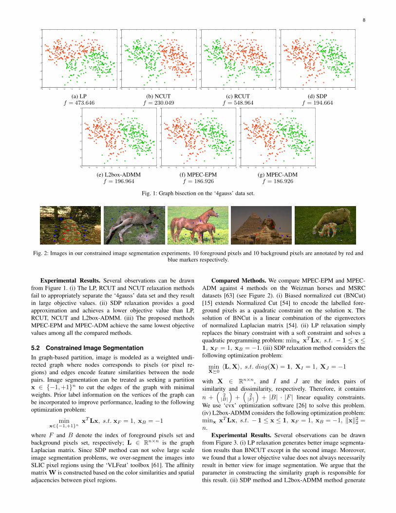
Fig. 1: Graph bisection on the ‘4gauss’ data set.

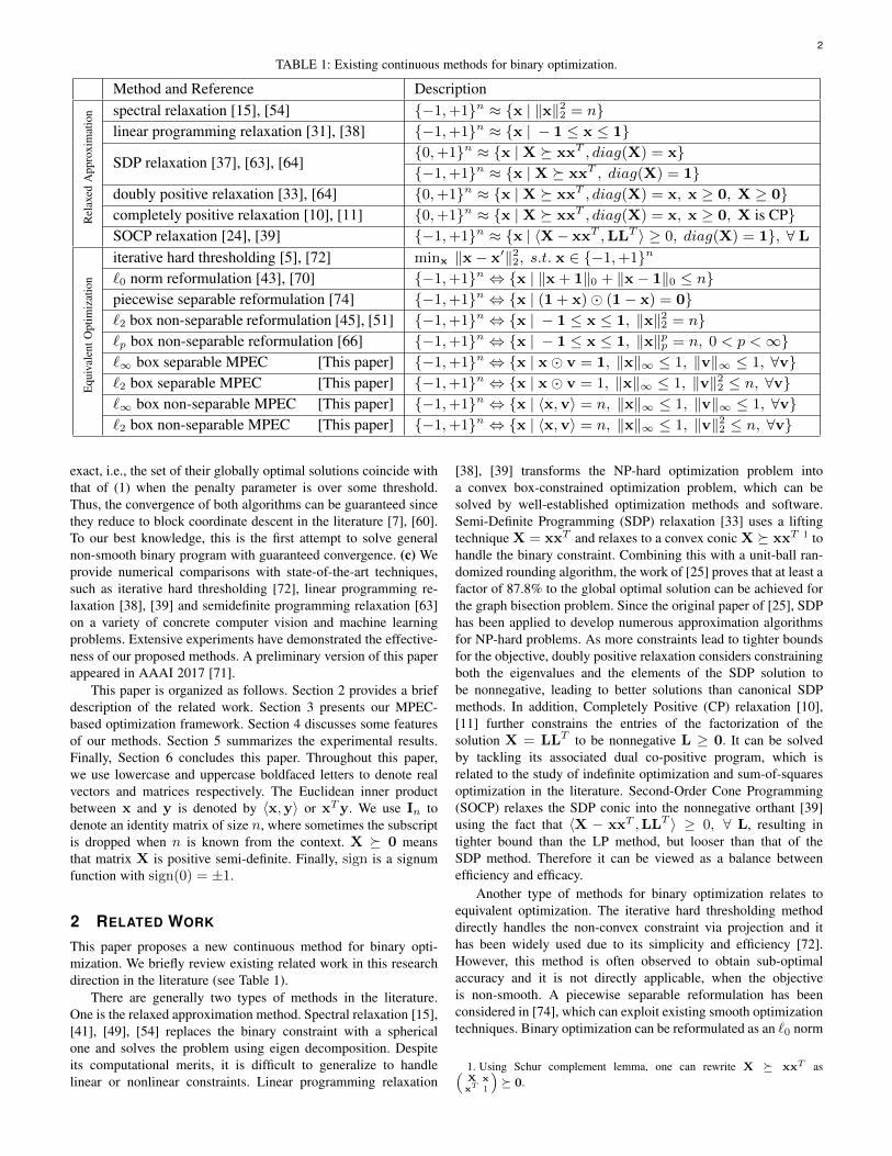
Fig. 2: Images in our constrained image segmentation experiments. 10 foreground pixels and 10 background pixels are annotated by red andblue markers respectively.

Experimental Results. Several observations can be drawnfrom Figure 1. (i) The LP, RCUT and NCUT relaxation methodsfail to appropriately separate the ‘4gauss’ data set and they resultin large objective values. (ii) SDP relaxation provides a goodapproximation and achieves a lower objective value than LP,RCUT, NCUT and L2box-ADMM. (iii) The proposed methodsMPEC-EPM and MPEC-ADM achieve the same lowest objectivevalues among all the compared methods.

5.2 Constrained Image SegmentationIn graph-based partition, image is modeled as a weighted undi-rected graph where nodes corresponds to pixels (or pixel re-gions) and edges encode feature similarities between the nodepairs. Image segmentation can be treated as seeking a partitionx ∈ −1,+1n to cut the edges of the graph with minimalweights. Prior label information on the vertices of the graph canbe incorporated to improve performance, leading to the followingoptimization problem:

minx∈−1,+1n

xTLx, s.t. xF = 1, xB = −1

where F and B denote the index of foreground pixels set andbackground pixels set, respectively; L ∈ Rn×n is the graphLaplacian matrix. Since SDP method can not solve large scaleimage segmentation problems, we over-segment the images intoSLIC pixel regions using the ‘VLFeat’ toolbox [61]. The affinitymatrix W is constructed based on the color similarities and spatialadjacencies between pixel regions.

Compared Methods. We compare MPEC-EPM and MPEC-ADM against 4 methods on the Weizman horses and MSRCdatasets [63] (see Figure 2). (i) Biased normalized cut (BNCut)[15] extends Normalized Cut [54] to encode the labelled fore-ground pixels as a quadratic constraint on the solution x. Thesolution of BNCut is a linear combination of the eigenvectorsof normalized Laplacian matrix [54]. (ii) LP relaxation simplyreplaces the binary constraint with a soft constraint and solves aquadratic programming problem: minx xTLx, s.t. − 1 ≤ x ≤1, xF = 1, xB = −1. (iii) SDP relaxation method considers thefollowing optimization problem:

minX0

〈L,X〉, s.t. diag(X) = 1, XI = 1, XJ = −1

with X ∈ Rn×n, and I and J are the index pairs ofsimilarity and dissimilarity, respectively. Therefore, it containsn +

(2|B|

)+(

2|F |

)+ |B| · |F | linear equality constraints.

We use ‘cvx’ optimization software [26] to solve this problem.(iv) L2box-ADMM considers the following optimization problem:minx xTLx, s.t. − 1 ≤ x ≤ 1, xF = 1, xB = −1, ‖x‖22 =n.

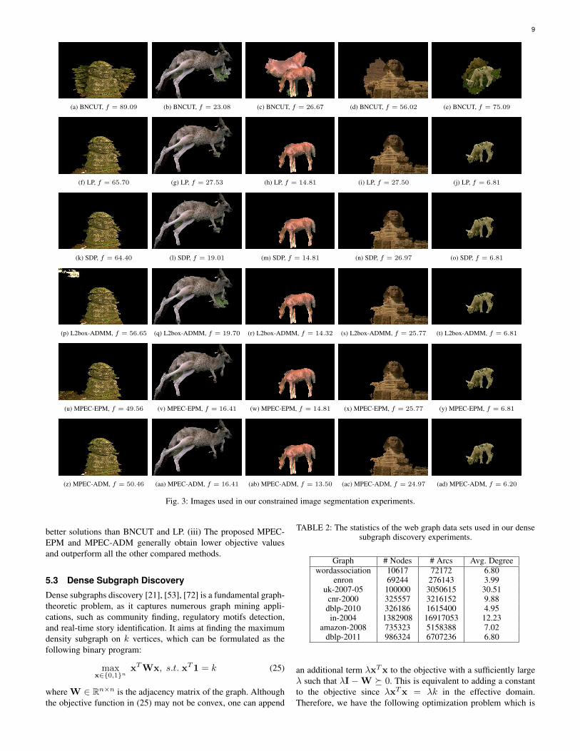
Experimental Results. Several observations can be drawnfrom Figure 3. (i) LP relaxation generates better image segmenta-tion results than BNCUT except in the second image. Moreover,we found that a lower objective value does not always necessarilyresult in better view for image segmentation. We argue that theparameter in constructing the similarity graph is responsible forthis result. (ii) SDP method and L2box-ADMM method generate

9

(a) BNCUT, f = 89.09 (b) BNCUT, f = 23.08 (c) BNCUT, f = 26.67 (d) BNCUT, f = 56.02 (e) BNCUT, f = 75.09

(f) LP, f = 65.70 (g) LP, f = 27.53 (h) LP, f = 14.81 (i) LP, f = 27.50 (j) LP, f = 6.81

(k) SDP, f = 64.40 (l) SDP, f = 19.01 (m) SDP, f = 14.81 (n) SDP, f = 26.97 (o) SDP, f = 6.81

(p) L2box-ADMM, f = 56.65 (q) L2box-ADMM, f = 19.70 (r) L2box-ADMM, f = 14.32 (s) L2box-ADMM, f = 25.77 (t) L2box-ADMM, f = 6.81

(u) MPEC-EPM, f = 49.56 (v) MPEC-EPM, f = 16.41 (w) MPEC-EPM, f = 14.81 (x) MPEC-EPM, f = 25.77 (y) MPEC-EPM, f = 6.81

(z) MPEC-ADM, f = 50.46 (aa) MPEC-ADM, f = 16.41 (ab) MPEC-ADM, f = 13.50 (ac) MPEC-ADM, f = 24.97 (ad) MPEC-ADM, f = 6.20

Fig. 3: Images used in our constrained image segmentation experiments.

better solutions than BNCUT and LP. (iii) The proposed MPEC-EPM and MPEC-ADM generally obtain lower objective valuesand outperform all the other compared methods.

5.3 Dense Subgraph Discovery

Dense subgraphs discovery [21], [53], [72] is a fundamental graph-theoretic problem, as it captures numerous graph mining appli-cations, such as community finding, regulatory motifs detection,and real-time story identification. It aims at finding the maximumdensity subgraph on k vertices, which can be formulated as thefollowing binary program:

maxx∈0,1n

xTWx, s.t. xT1 = k (25)

where W ∈ Rn×n is the adjacency matrix of the graph. Althoughthe objective function in (25) may not be convex, one can append

TABLE 2: The statistics of the web graph data sets used in our densesubgraph discovery experiments.

Graph # Nodes # Arcs Avg. Degreewordassociation 10617 72172 6.80

enron 69244 276143 3.99uk-2007-05 100000 3050615 30.51

cnr-2000 325557 3216152 9.88dblp-2010 326186 1615400 4.95in-2004 1382908 16917053 12.23

amazon-2008 735323 5158388 7.02dblp-2011 986324 6707236 6.80

an additional term λxTx to the objective with a sufficiently largeλ such that λI−W 0. This is equivalent to adding a constantto the objective since λxTx = λk in the effective domain.Therefore, we have the following optimization problem which is

10

100 1000 2000 3000 4000 5000

2

4

6

8

10

12

14

cardinality

de

nsi

ty

(a) wordassociation

100 1000 2000 3000 4000 5000

20

25

30

35

40

45

50

cardinality

de

nsi

ty

(b) uk-2007-05

100 1000 2000 3000 4000 5000

20

40

60

80

100

cardinality

de

nsi

ty

(c) uk-2014-tpd

100 1000 2000 3000 4000 5000

10

20

30

40

50

60

cardinality

de

nsi

ty

(d) in-2004

100 1000 2000 3000 4000 5000

10

20

30

40

50

60

70

cardinality

de

nsi

ty

(e) amazon-2008

100 1000 2000 3000 4000 5000

50

100

150

200

250

300

350

400

cardinality

de

nsi

ty

(f) enron

100 1000 2000 3000 4000 5000

3

4

5

6

7

8

cardinality

de

nsi

ty

(g) cnr-2000

100 1000 2000 3000 4000 5000

20

40

60

80

100

cardinality

de

nsi

ty

(h) dblp-2010

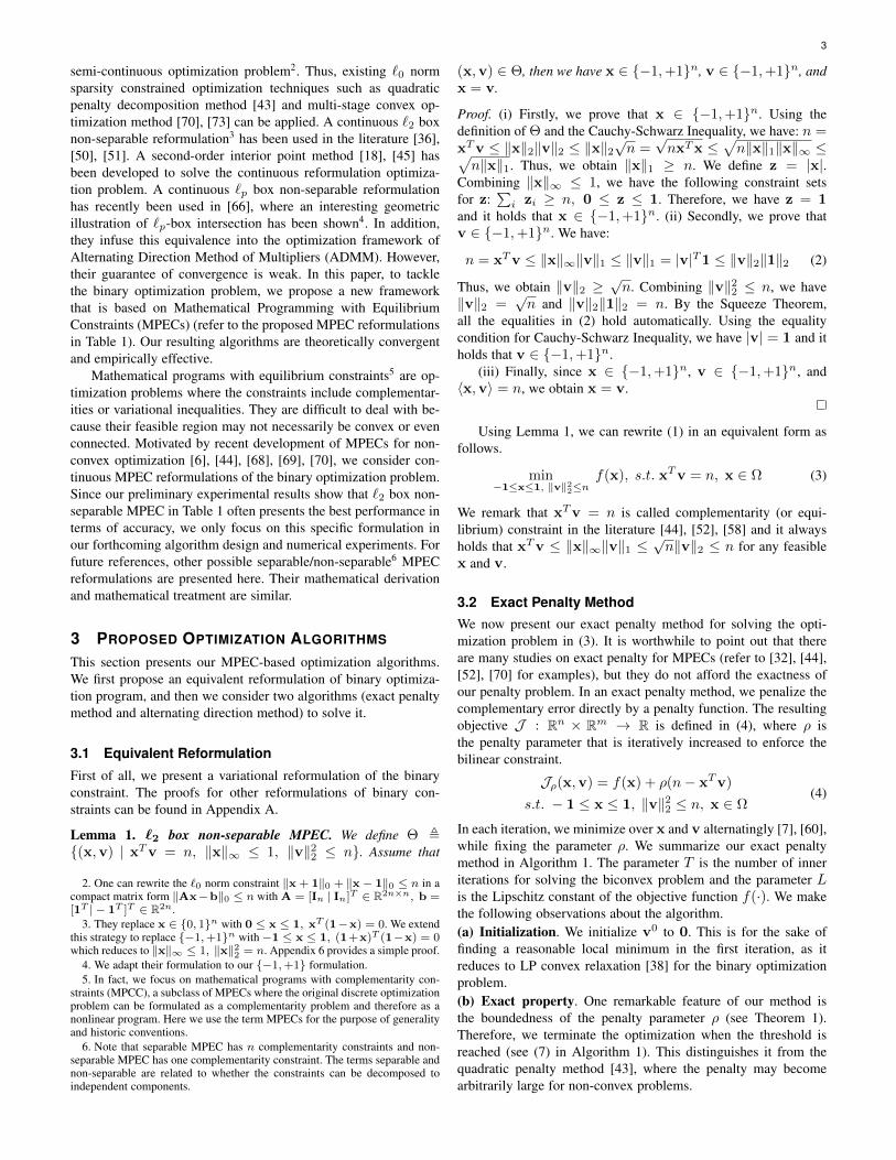
Fig. 4: Experimental results for dense subgraph discovery.

equivalent to (25):

minx∈0,1n

xT (λI−W)x, s.t. xT1 = k

In the experiments, λ is set to the largest eigenvalue of W.Compared Methods. We compare MPEC-EPM and MPEC-

ADM against 5 methods on 8 datasets15 (see Table 2). (i) Feige’sgreedy algorithm (GEIGE) [21] is included in our comparisons.This method is known to achieve the best approximation ratiofor general k. (ii) Ravi’s greedy algorithm (RAVI) [53] startsfrom a heaviest edge and repeatedly adds a vertex to the currentsubgraph to maximize the weight of the resulting new subgraph.It has asymptotic performance guarantee of π/2 when the weightssatisfy the triangle inequality. (iii) LP relaxation solves a cappedsimplex problem by standard quadratic programming technique:minx xT (λI − W)x, s.t. 0 ≤ x ≤ 1, xT1 = k. (iii)L2box-ADMM solves a spherical constraint optimization prob-lem: minx xT (λI − W)x, s.t. 0 ≤ x ≤ 1, xT1 =k, ‖2x − 1‖22 = n. (iv) Truncated Power Method (TPM) [72]considers an iterative procedure that combines power iteration andhard-thresholding truncation. It works by greedily decreasing theobjective while maintaining the desired binary property for theintermediate solutions. We use the code16 provided by the authors.As suggested in [72], the initial solution is set to the indicatorvector of the vertices with the top k weighted degrees of the graphin our experiments.

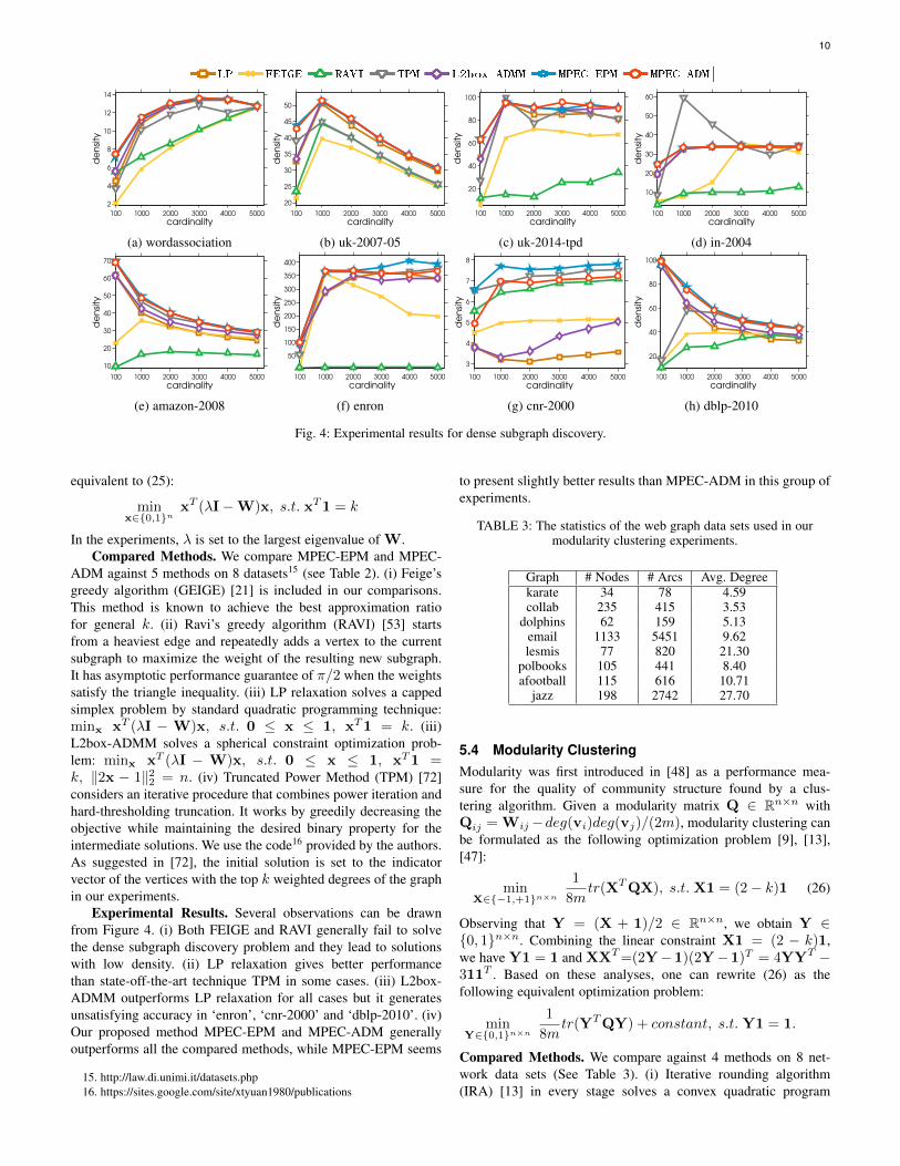
Experimental Results. Several observations can be drawnfrom Figure 4. (i) Both FEIGE and RAVI generally fail to solvethe dense subgraph discovery problem and they lead to solutionswith low density. (ii) LP relaxation gives better performancethan state-off-the-art technique TPM in some cases. (iii) L2box-ADMM outperforms LP relaxation for all cases but it generatesunsatisfying accuracy in ‘enron’, ‘cnr-2000’ and ‘dblp-2010’. (iv)Our proposed method MPEC-EPM and MPEC-ADM generallyoutperforms all the compared methods, while MPEC-EPM seems

15. http://law.di.unimi.it/datasets.php16. https://sites.google.com/site/xtyuan1980/publications

to present slightly better results than MPEC-ADM in this group ofexperiments.

TABLE 3: The statistics of the web graph data sets used in ourmodularity clustering experiments.

Graph # Nodes # Arcs Avg. Degreekarate 34 78 4.59collab 235 415 3.53

dolphins 62 159 5.13email 1133 5451 9.62lesmis 77 820 21.30

polbooks 105 441 8.40afootball 115 616 10.71

jazz 198 2742 27.70

5.4 Modularity ClusteringModularity was first introduced in [48] as a performance mea-sure for the quality of community structure found by a clus-tering algorithm. Given a modularity matrix Q ∈ Rn×n withQij = Wij−deg(vi)deg(vj)/(2m), modularity clustering canbe formulated as the following optimization problem [9], [13],[47]:

minX∈−1,+1n×n

1

8mtr(XTQX), s.t. X1 = (2− k)1 (26)

Observing that Y = (X + 1)/2 ∈ Rn×n, we obtain Y ∈0, 1n×n. Combining the linear constraint X1 = (2 − k)1,we have Y1 = 1 and XXT=(2Y−1)(2Y−1)T = 4YYT −311T . Based on these analyses, one can rewrite (26) as thefollowing equivalent optimization problem:

minY∈0,1n×n

1

8mtr(YTQY) + constant, s.t. Y1 = 1.

Compared Methods. We compare against 4 methods on 8 net-work data sets (See Table 3). (i) Iterative rounding algorithm(IRA) [13] in every stage solves a convex quadratic program

11

5 10 15 20 25 30

0.34

0.36

0.38

0.4

0.42

cardinality

de

nsi

ty

(a) karate

5 10 15 20 25 30

0.4

0.5

0.6

0.7

0.8

cardinality

de

nsi

ty

(b) collab

5 10 15 20 25 30

0.4

0.45

0.5

0.55

cardinality

de

nsi

ty

(c) dolphins

5 10 15 20 25 30

0.3

0.35

0.4

0.45

0.5

0.55

cardinality

de

nsi

ty

(d) email

5 10 15 20 25 30

0.35

0.4

0.45

0.5

0.55

cardinality

de

nsi

ty

(e) lesmis

5 10 15 20 25 30

0.42

0.44

0.46

0.48

0.5

0.52

0.54

cardinality

de

nsi

ty

(f) polbooks

5 10 15 20 25 30

0.35

0.4

0.45

0.5

0.55

0.6

cardinality

de

nsi

ty

(g) afootball

5 10 15 20 25 30

0.3

0.35

0.4

0.45

cardinality

de

nsi

ty

(h) jazz

Fig. 5: Experimental results for modularity clustering.

and picks a fixed number of the vertices with largest values toassign to the cluster. However, such heuristic algorithm does nothave any convergence guarantee. We use the code provided bythe authors17 and set the parameter ρ = 0.5 in this method.(ii) LP relaxation solves a capped simplex problem. (iii) L2box-ADMM solves a spherical constrained optimization problem. (iv)Iterative Hard Thresholding (IHT) considers setting the currentsolution to the indicator vector of its top-k entries while decreasingthe objective function. Due to its suboptimal performance in ourprevious experiment, LP relaxation is used as its initialization.

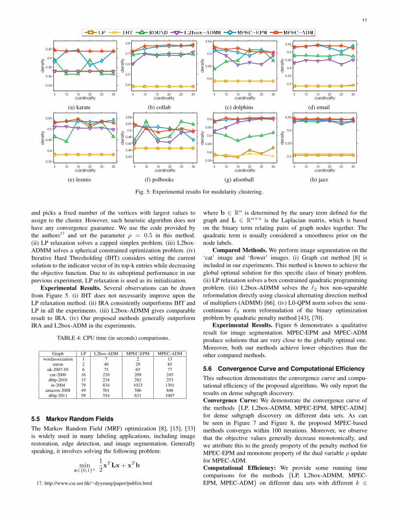
Experimental Results. Several observations can be drawnfrom Figure 5. (i) IHT does not necessarily improve upon theLP relaxation method. (ii) IRA consistently outperforms IHT andLP in all the experiments. (iii) L2box-ADMM gives comparableresult to IRA. (iv) Our proposed methods generally outperformIRA and L2box-ADM in the experiments.

TABLE 4: CPU time (in seconds) comparisons.

Graph LP L2box-ADM MPEC-EPM MPEC-ADMwordassociation 1 7 2 13

enron 2 40 29 85uk-2007-05 6 75 65 77

cnr-2000 16 210 209 245dblp-2010 15 234 282 253in-2004 79 834 1023 1301

amazon-2008 49 501 586 846dblp-2011 59 554 621 1007

5.5 Markov Random FieldsThe Markov Random Field (MRF) optimization [8], [15], [33]is widely used in many labeling applications, including imagerestoration, edge detection, and image segmentation. Generallyspeaking, it involves solving the following problem:

minx∈0,1n

1

2xTLx + xTb

17. http://www.cse.ust.hk/∼dyyeung/paper/publist.html

where b ∈ Rn is determined by the unary term defined for thegraph and L ∈ Rn×n is the Laplacian matrix, which is basedon the binary term relating pairs of graph nodes together. Thequadratic term is usually considered a smoothness prior on thenode labels.

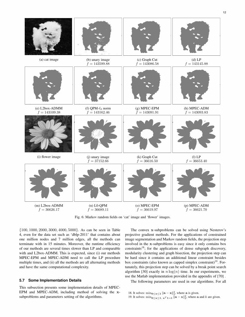
Compared Methods. We perform image segmentation on the‘cat’ image and ‘flower’ images. (i) Graph cut method [8] isincluded in our experiments. This method is known to achieve theglobal optimal solution for this specific class of binary problem.(ii) LP relaxation solves a box constrained quadratic programmingproblem. (iii) L2box-ADMM solves the `2 box non-separablereformulation directly using classical alternating direction methodof multipliers (ADMM) [66]. (iv) L0-QPM norm solves the semi-continuous `0 norm reformulation of the binary optimizationproblem by quadratic penalty method [43], [70].

Experimental Results. Figure 6 demonstrates a qualitativeresult for image segmentation. MPEC-EPM and MPEC-ADMproduce solutions that are very close to the globally optimal one.Moreover, both our methods achieve lower objectives than theother compared methods.

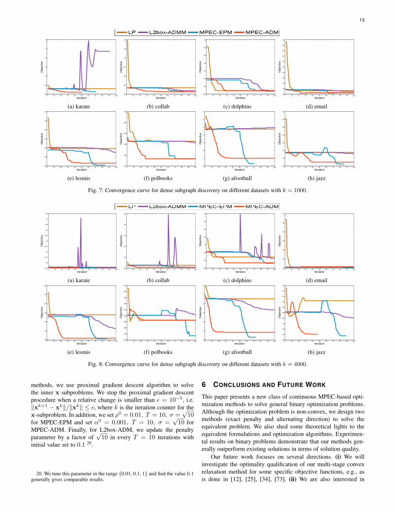
5.6 Convergence Curve and Computational EfficiencyThis subsection demonstrates the convergence curve and compu-tational efficiency of the proposed algorithms. We only report theresults on dense subgraph discovery.Convergence Curve: We demonstrate the convergence curve ofthe methods LP, L2box-ADMM, MPEC-EPM, MPEC-ADMfor dense subgraph discovery on different data sets. As canbe seen in Figure 7 and Figure 8, the proposed MPEC-basedmethods converges within 100 iterations. Moreover, we observethat the objective values generally decrease monotonically, andwe attribute this to the greedy property of the penalty method forMPEC-EPM and monotone property of the dual variable ρ updatefor MPEC-ADM.Computational Efficiency: We provide some running timecomparisons for the methods LP, L2box-ADMM, MPEC-EPM, MPEC-ADM on different data sets with different k ∈

12

(a) cat image (b) unary imagef = 143599.88

(c) Graph Cutf = 143086.58

(d) LPf = 143145.88

(e) L2box-ADMMf = 143109.38

(f) QPM-`0 normf = 143162.46

(g) MPEC-EPMf = 143091.91

(h) MPEC-ADMf = 143093.83

(i) flower image (j) unary imagef = 37152.66

(k) Graph Cutf = 36616.50

(l) LPf = 36653.40

(m) L2box-ADMMf = 36626.17

(n) L0-QPMf = 36689.11

(o) MPEC-EPMf = 36619.97

(p) MPEC-ADMf = 36621.70

Fig. 6: Markov random fields on ‘cat’ image and ‘flower’ images.

100, 1000, 2000, 3000, 4000, 5000. As can be seen in Table4, even for the data set such as ‘dblp-2011’ that contains aboutone million nodes and 7 million edges, all the methods canterminate with in 15 minutes. Moreover, the runtime efficiencyof our methods are several times slower than LP and comparablewith and L2box-ADMM. This is expected, since (i) our methodsMPEC-EPM and MPEC-ADM need to call the LP proceduremultiple times, and (ii) all the methods are all alternating methodsand have the same computational complexity.

5.7 Some Implementation Details

This subsection presents some implementation details of MPEC-EPM and MPEC-ADM, including method of solving the x-subproblems and parameters setting of the algorithms.

The convex x-subproblems can be solved using Nesterov’sprojective gradient methods. For the applications of constrainedimage segmentation and Markov random fields, the projection stepinvolved in the x-subproblems is easy since it only contains boxconstraints18; for the applications of dense subgraph discovery,modularity clustering and graph bisection, the projection step canbe hard since it contains an additional linear constraint besidesbox constraints (also known as capped simplex constraint)19. For-tunately, this projection step can be solved by a break point searchalgorithm [30] exactly in n log(n) time. In our experiments, weuse the Matlab implementation provided in the appendix of [70] .

The following parameters are used in our algorithms. For all

18. It solves: min0≤x≤1 ‖a− x‖22, where a is given.19. It solves: min0≤x≤1, xT 1=k ‖a− x‖22, where a and k are given.

13

0 10 20 30 40 50 60 70 80 90 100−12

−10

−8

−6

−4

−2

0

Iteration

Obj

ectiv

e

(a) karate

0 10 20 30 40 50 60 70 80 90 100−52

−50

−48

−46

−44

−42

−40

Iteration

Obj

ectiv

e

(b) collab

0 10 20 30 40 50 60 70 80 90 100−100

−90

−80

−70

−60

−50

−40

−30

Iteration

Obj

ectiv

e

(c) dolphins

0 10 20 30 40 50 60 70 80 90 100−34

−32

−30

−28

−26

−24

−22

−20

−18

−16

−14

Iteration

Obj

ectiv

e

(d) email

0 10 20 30 40 50 60 70 80 90 100−50

−45

−40

−35

−30

−25

−20

Iteration

Obj

ectiv

e

(e) lesmis

0 10 20 30 40 50 60 70 80 90 100−400

−350

−300

−250

−200

−150

Iteration

Obj

ectiv

e

(f) polbooks

0 10 20 30 40 50 60 70 80 90 100−8

−7

−6

−5

−4

−3

−2

−1

Iteration

Obj

ectiv

e

(g) afootball

0 10 20 30 40 50 60 70 80 90 100−80

−70

−60

−50

−40

−30

−20

−10

Iteration

Obj

ectiv

e

(h) jazz

Fig. 7: Convergence curve for dense subgraph discovery on different datasets with k = 1000.

0 10 20 30 40 50 60 70 80 90 100−13.5

−13

−12.5

−12

−11.5

−11

−10.5

−10

−9.5

−9

−8.5

Iteration

Obj

ectiv

e

(a) karate

0 10 20 30 40 50 60 70 80 90 100−35

−30

−25

−20

−15

−10

Iteration

Obj

ectiv

e

(b) collab

0 10 20 30 40 50 60 70 80 90 100−100

−90

−80

−70

−60

−50

−40

−30

Iteration

Obj

ectiv

e

(c) dolphins

0 10 20 30 40 50 60 70 80 90 100−34

−32

−30

−28

−26

−24

−22

Iteration

Obj

ectiv

e(d) email

0 10 20 30 40 50 60 70 80 90 100−32

−30

−28

−26

−24

−22

−20

Iteration

Obj

ectiv

e

(e) lesmis

0 10 20 30 40 50 60 70 80 90 100−420

−400

−380

−360

−340

−320

−300

−280

−260

−240

Iteration

Obj

ectiv

e

(f) polbooks

0 10 20 30 40 50 60 70 80 90 100−8

−7

−6

−5

−4

−3

−2

Iteration

Obj

ectiv

e

(g) afootball

0 10 20 30 40 50 60 70 80 90 100−48

−46

−44

−42

−40

−38

−36

−34

−32

−30

−28

Iteration

Obj

ectiv

e

(h) jazz

Fig. 8: Convergence curve for dense subgraph discovery on different datasets with k = 4000.

methods, we use proximal gradient descent algorithm to solvethe inner x subproblems. We stop the proximal gradient descentprocedure when a relative change is smaller than ε = 10−5, i.e.‖xk+1 − xk‖/‖xk‖ ≤ ε, where k is the iteration counter for thex-subproblem. In addition, we set ρ0 = 0.01, T = 10, σ =

√10

for MPEC-EPM and set α0 = 0.001, T = 10, σ =√

10 forMPEC-ADM. Finally, for L2box-ADM, we update the penaltyparameter by a factor of

√10 in every T = 10 iterations with

initial value set to 0.1 20.

20. We tune this parameter in the range 0.01, 0.1, 1 and find the value 0.1generally gives comparable results.

6 CONCLUSIONS AND FUTURE WORK

This paper presents a new class of continuous MPEC-based opti-mization methods to solve general binary optimization problems.Although the optimization problem is non-convex, we design twomethods (exact penalty and alternating direction) to solve theequivalent problem. We also shed some theoretical lights to theequivalent formulations and optimization algorithms. Experimen-tal results on binary problems demonstrate that our methods gen-erally outperform existing solutions in terms of solution quality.

Our future work focuses on several directions. (i) We willinvestigate the optimality qualification of our multi-stage convexrelaxation method for some specific objective functions, e.g., asis done in [12], [25], [34], [73]. (ii) We are also interested in

14

extending the proposed algorithms to solve orthogonality andspherical optimization problems [14], [65] in computer vision andmachine learning.

ACKNOWLEDGMENTS

We would like to thank Prof. Shaohua Pan and Dr. Li Shen (SouthChina University of Technology) for their valuable discussions onthe MPEC techniques. Research reported in this publication wassupported by competitive research funding from King AbdullahUniversity of Science and Technology (KAUST).

REFERENCES

[1] B. P. Ames. Guaranteed clustering and biclustering via semidefiniteprogramming. Mathematical Programming, 147(1-2):429–465, 2014.

[2] B. P. Ames. Guaranteed recovery of planted cliques and dense subgraphsby convex relaxation. Journal of Optimization Theory and Applications,167(2):653–675, 2015.

[3] B. P. W. Ames and S. A. Vavasis. Nuclear norm minimization forthe planted clique and biclique problems. Mathematical Programming,129(1):69–89, 2011.

[4] B. P. W. Ames and S. A. Vavasis. Convex optimization for the plantedk-disjoint-clique problem. Mathematical Programming, 143(1):299–337,2014.

[5] A. Beck and Y. C. Eldar. Sparsity constrained nonlinear optimization:Optimality conditions and algorithms. SIAM Journal on Optimization(SIOPT), 23(3):1480–1509, 2013.

[6] S. Bi, X. Liu, and S. Pan. Exact penalty decomposition method forzero-norm minimization based on mpec formulation. SIAM Journal onScientific Computing (SISC), 36(4):A1451–A1477, 2014.

[7] J. Bolte, S. Sabach, and M. Teboulle. Proximal alternating linearizedminimization for nonconvex and nonsmooth problems. MathematicalProgramming, 146(1-2):459–494, 2014.

[8] Y. Boykov, O. Veksler, and R. Zabih. Fast approximate energy minimiza-tion via graph cuts. IEEE Transactions on Pattern Analysis and MachineIntelligence (TPAMI), 23(11):1222–1239, 2001.

[9] U. Brandes, D. Delling, M. Gaertler, R. Gorke, M. Hoefer, Z. Nikoloski,and D. Wagner. On modularity clustering. IEEE Transactions onKnowledge and Data Engineering (TKDE), 20(2):172–188, 2008.

[10] S. Burer. On the copositive representation of binary and continuous non-convex quadratic programs. Mathematical Programming, 120(2):479–495, 2009.

[11] S. Burer. Optimizing a polyhedral-semidefinite relaxation of completelypositive programs. Mathematical Programming Computation, 2(1):1–19,2010.

[12] E. J. Candes, X. Li, and M. Soltanolkotabi. Phase retrieval via wirtingerflow: Theory and algorithms. IEEE Transactions on Information Theory,61(4):1985–2007, 2015.

[13] E. Y. K. Chan and D. Yeung. A convex formulation of modularity maxi-mization for community detection. In International Joint Conference onArtificial Intelligence (IJCAI), pages 2218–2225, 2011.

[14] W. Chen, H. Ji, and Y. You. An augmented lagrangian method for l1-regularized optimization problems with orthogonality constraints. SIAMJournal on Scientific Computing (SISC), 38(4):B570–B592, 2016.

[15] T. Cour and J. Shi. Solving markov random fields with spectralrelaxation. In International Conference on Artificial Intelligence andStatistics (AISTATS), volume 2, page 15, 2007.

[16] T. Cour, P. Srinivasan, and J. Shi. Balanced graph matching. NeuralInformation Processing Systems (NIPS), 19:313, 2007.

[17] M. A. Davenport, Y. Plan, E. van den Berg, and M. Wootters. 1-bit matrixcompletion. Information and Inference, 3(3):189–223, 2014.

[18] M. De Santis and F. Rinaldi. Continuous reformulations for zero–oneprogramming problems. Journal of Optimization Theory and Applica-tions, 153(1):75–84, 2012.

[19] G. Di Pillo. Exact penalty methods. In Algorithms for ContinuousOptimization, pages 209–253. Springer, 1994.

[20] G. Di Pillo and L. Grippo. Exact penalty functions in constrainedoptimization. SIAM Journal on Control and Optimization, 27(6):1333–1360, 1989.

[21] U. Feige, D. Peleg, and G. Kortsarz. The dense k-subgraph problem.Algorithmica, 29(3):410–421, 2001.

[22] F. Fogel, R. Jenatton, F. R. Bach, and A. d’Aspremont. Convexrelaxations for permutation problems. SIAM Journal on Matrix Analysisand Applications (SIMAX), 36(4):1465–1488, 2015.

[23] W. Gander, G. H. Golub, and U. von Matt. A constrained eigenvalueproblem. Linear Algebra and its applications, 114:815–839, 1989.

[24] B. Ghaddar, J. C. Vera, and M. F. Anjos. Second-order cone relaxationsfor binary quadratic polynomial programs. SIAM Journal on Optimiza-tion (SIOPT), 21(1):391–414, 2011.

[25] M. X. Goemans and D. P. Williamson. Improved approximation algo-rithms for maximum cut and satisfiability problems using semidefiniteprogramming. Journal of the ACM, 42(6):1115–1145, 1995.

[26] M. Grant and S. Boyd. CVX: Matlab software for disciplined convexprogramming, version 2.1. http://cvxr.com/cvx, Mar. 2014.

[27] S.-P. Han and O. L. Mangasarian. Exact penalty functions in nonlinearprogramming. Mathematical programming, 17(1):251–269, 1979.

[28] B. He and X. Yuan. On the O(1/n) convergence rate of the douglas-rachford alternating direction method. SIAM Journal on NumericalAnalysis (SINUM), 50(2):700–709, 2012.

[29] L. He, C.-T. Lu, J. Ma, J. Cao, L. Shen, and P. S. Yu. Joint communityand structural hole spanner detection via harmonic modularity. InACM SIGKDD Conferences on Knowledge Discovery and Data Mining(SIGKDD). ACM, 2016.

[30] R. Helgason, J. Kennington, and H. Lall. A polynomially boundedalgorithm for a singly constrained quadratic program. MathematicalProgramming, 18(1):338–343, 1980.

[31] C.-J. Hsieh, N. Natarajan, and I. S. Dhillon. Pu learning for matrixcompletion. In International Conference on Machine Learning (ICML),pages 2445–2453, 2015.

[32] X. Hu and D. Ralph. Convergence of a penalty method for mathematicalprogramming with complementarity constraints. Journal of OptimizationTheory and Applications, 123(2):365–390, 2004.

[33] Q. Huang, Y. Chen, and L. J. Guibas. Scalable semidefinite relaxationfor maximum A posterior estimation. In International Conference onMachine Learning (ICML), pages 64–72, 2014.

[34] P. Jain, P. Netrapalli, and S. Sanghavi. Low-rank matrix completion usingalternating minimization. In ACM Symposium on Theory of Computing(STOC), pages 665–674, 2013.

[35] A. Joulin, F. R. Bach, and J. Ponce. Discriminative clustering for imageco-segmentation. In IEEE Conference on Computer Vision and Pattern(CVPR), pages 1943–1950, 2010.

[36] B. Kalantari and J. B. Rosen. Penalty for zero–one integer equivalentproblem. Mathematical Programming, 24(1):229–232, 1982.

[37] J. Keuchel, C. Schnorr, C. Schellewald, and D. Cremers. Binary parti-tioning, perceptual grouping, and restoration with semidefinite program-ming. IEEE Transactions on Pattern Analysis and Machine Intelligence(TPAMI), 25(11):1364–1379, 2003.

[38] N. Komodakis and G. Tziritas. Approximate labeling via graph cutsbased on linear programming. IEEE Transactions on Pattern Analysisand Machine Intelligence (TPAMI), 29(8):1436–1453, 2007.

[39] M. P. Kumar, V. Kolmogorov, and P. H. S. Torr. An analysis of convexrelaxations for MAP estimation of discrete mrfs. Journal of MachineLearning Research (JMLR), 10:71–106, 2009.

[40] R. Lai and S. Osher. A splitting method for orthogonality constrainedproblems. Journal of Scientific Computing, 58(2):431–449, 2014.

[41] G. Lin, C. Shen, D. Suter, and A. van den Hengel. A general two-step approach to learning-based hashing. In International Conference onComputer Vision (ICCV), pages 2552–2559, 2013.

[42] W. Liu, J. Wang, S. Kumar, and S. Chang. Hashing with graphs.In International Conference on Machine Learning (ICML), pages 1–8,2011.

[43] Z. Lu and Y. Zhang. Sparse approximation via penalty decompositionmethods. SIAM Journal on Optimization (SIOPT), 23(4):2448–2478,2013.

[44] Z.-Q. Luo, J.-S. Pang, and D. Ralph. Mathematical programs withequilibrium constraints. Cambridge University Press, 1996.

[45] W. Murray and K. Ng. An algorithm for nonlinear optimization problemswith binary variables. Computational Optimization and Applications,47(2):257–288, 2010.

[46] Y. E. Nesterov. Introductory lectures on convex optimization: a basiccourse, volume 87 of Applied Optimization. Kluwer Academic Publish-ers, 2003.

[47] M. E. Newman. Modularity and community structure in networks.Proceedings of the national academy of sciences, 103(23):8577–8582,2006.

[48] M. E. Newman and M. Girvan. Finding and evaluating communitystructure in networks. Physical review E, 69(2):026113, 2004.

[49] C. Olsson, A. P. Eriksson, and F. Kahl. Solving large scale binaryquadratic problems: Spectral methods vs. semidefinite programming. InIEEE Conference on Computer Vision and Pattern Recognition (CVPR),pages 1–8. IEEE, 2007.

[50] P. M. Pardalos and J. B. Rosen. Constrained Global Optimization:Algorithms and Applications. Springer-Verlag New York, Inc., New York,NY, USA, 1987.

[51] M. Raghavachari. On connections between zero-one integer program-ming and concave programming under linear constraints. Operations

15

Research, 17(4):680–684, 1969.[52] D. Ralph and S. J. Wright. Some properties of regularization and

penalization schemes for mpecs. Optimization Methods and Software,19(5):527–556, 2004.

[53] S. S. Ravi, D. J. Rosenkrantz, and G. K. Tayi. Heuristic and special casealgorithms for dispersion problems. Operations Research, 42(2):299–310, 1994.

[54] J. Shi and J. Malik. Normalized cuts and image segmentation. IEEETransactions on Pattern Analysis and Machine Intelligence (TPAMI),22(8):888–905, 2000.

[55] X. Shi, H. Ling, J. Xing, and W. Hu. Multi-target tracking by rank-1 tensor approximation. In IEEE Conference on Computer Vision andPattern Recognition (CVPR), pages 2387–2394, 2013.

[56] F. Shokrollahi Yancheshmeh, K. Chen, and J.-K. Kamarainen. Unsu-pervised visual alignment with similarity graphs. In IEEE Conferenceon Computer Vision and Pattern Recognition (CVPR), pages 2901–2908,2015.

[57] A. Shrivastava, M. Rastegari, S. Shekhar, R. Chellappa, and L. S. Davis.Class consistent multi-modal fusion with binary features. In IEEEConference on Computer Vision and Pattern Recognition (CVPR), pages2282–2291, 2015.

[58] S. Steffensen and M. Ulbrich. A new relaxation scheme for mathematicalprograms with equilibrium constraints. SIAM Journal on Optimization(SIOPT), 20(5):2504–2539, 2010.

[59] A. Toshev, J. Shi, and K. Daniilidis. Image matching via saliency regioncorrespondences. In IEEE Conference on Computer Vision and PatternRecognition (CVPR), pages 1–8. IEEE, 2007.

[60] P. Tseng. Convergence of a block coordinate descent method fornondifferentiable minimization. Journal of Optimization Theory andApplications, 109(3):475–494, 2001.

[61] A. Vedaldi and B. Fulkerson. Vlfeat: An open and portable libraryof computer vision algorithms. In ACM International Conference onMultimedia (ACM MM), pages 1469–1472, 2010.

[62] J. Wang, W. Liu, S. Kumar, and S. Chang. Learning to hash for indexingbig data - a survey. Proceedings of the IEEE, 104(1):34–57, 2016.

[63] P. Wang, C. Shen, A. van den Hengel, and P. Torr. Large-scalebinary quadratic optimization using semidefinite relaxation and applica-tions. IEEE Transactions on Pattern Analysis and Machine Intelligence(TPAMI), 2016.

[64] Z. Wen, D. Goldfarb, and W. Yin. Alternating direction augmentedlagrangian methods for semidefinite programming. Mathematical Pro-gramming Computation, 2(3):203–230, 2010.

[65] Z. Wen and W. Yin. A feasible method for optimization with orthogonal-ity constraints. Mathematical Programming, 142(1-2):397–434, 2013.

[66] B. Wu and B. Ghanem. $\ell p$-box ADMM: A versatile frameworkfor integer programming. In arXiv preprint, 2016.

[67] J. Yan, C. Zhang, H. Zha, W. Liu, X. Yang, and S. M. Chu. Discretehyper-graph matching. In IEEE Conference on Computer Vision andPattern Recognition (CVPR), pages 1520–1528, 2015.

[68] G. Yuan and B. Ghanem. `0tv: A new method for image restoration inthe presence of impulse noise. In IEEE Conference on Computer Visionand Pattern Recognition (CVPR), pages 5369–5377, 2015.

[69] G. Yuan and B. Ghanem. A proximal alternating direction methodfor semi-definite rank minimization. In AAAI Conference on ArtificialIntelligence (AAAI), 2016.

[70] G. Yuan and B. Ghanem. Sparsity constrained minimization via math-ematical programming with equilibrium constraints. In arXiv preprint,2016.

[71] G. Yuan and B. Ghanem. An exact penalty method for binary opti-mization based on MPEC formulation. In AAAI Conference on ArtificialIntelligence (AAAI), pages 2867–2875, 2017.

[72] X. Yuan and T. Zhang. Truncated power method for sparse eigenvalueproblems. Journal of Machine Learning Research (JMLR), 14(1):899–925, 2013.

[73] T. Zhang. Analysis of multi-stage convex relaxation for sparse regulariza-tion. The Journal of Machine Learning Research (JMLR), 11:1081–1107,2010.

[74] Z. Zhang, T. Li, C. Ding, and X. Zhang. Binary matrix factorization withapplications. In IEEE International Conference on Data Mining (ICDM),pages 391–400. IEEE, 2007.

[75] H. Zou and T. Hastie. Regularization and variable selection via theelastic net. Journal of the Royal Statistical Society: Series B (StatisticalMethodology), 67(2):301–320, 2005.

Ganzhao Yuan was born in Guangdong, China.He received his Ph.D. in School of Computer Sci-ence and Engineering, South China Universityof Technology (SCUT) in 2013. He is currently aresearch associate professor at School of Dataand Computer Science in Sun Yat-sen University(SYSU). His research interests primarily centeraround large-scale nonlinear optimization andits applications in computer vision and machinelearning. He has published papers in ICML,SIGKDD, AAAI, CVPR, VLDB, and ACM Trans-

actions on Database System (TODS).

Bernard Ghanem was born in Betroumine,Lebanon. He received his Ph.D. in Electricaland Computer Engineering from the Universityof Illinois at Urbana-Champaign (UIUC) in 2010.He is currently an assistant professor at KingAbdullah University of Science and Technology(KAUST), where he leads the Image and VideoUnderstanding Lab (IVUL). His research inter-ests focus on designing, implementing, and an-alyzing approaches to address computer visionproblems (e.g. object tracking and action recog-

nition/detection in video), especially at large-scale.

16

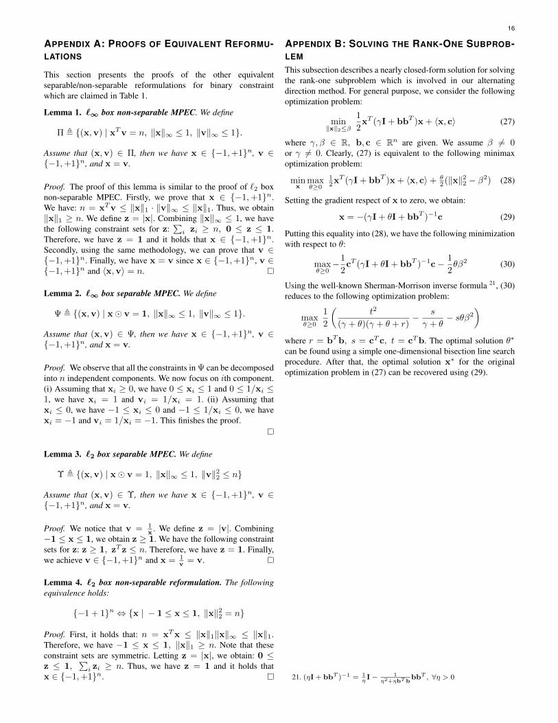
APPENDIX A: PROOFS OF EQUIVALENT REFORMU-LATIONS

This section presents the proofs of the other equivalentseparable/non-separable reformulations for binary constraintwhich are claimed in Table 1.

Lemma 1. `∞ box non-separable MPEC. We define

Π , (x,v) | xTv = n, ‖x‖∞ ≤ 1, ‖v‖∞ ≤ 1.

Assume that (x,v) ∈ Π, then we have x ∈ −1,+1n, v ∈−1,+1n, and x = v.

Proof. The proof of this lemma is similar to the proof of `2 boxnon-separable MPEC. Firstly, we prove that x ∈ −1,+1n.We have: n = xTv ≤ ‖x‖1 · ‖v‖∞ ≤ ‖x‖1. Thus, we obtain‖x‖1 ≥ n. We define z = |x|. Combining ‖x‖∞ ≤ 1, we havethe following constraint sets for z:

∑i zi ≥ n, 0 ≤ z ≤ 1.

Therefore, we have z = 1 and it holds that x ∈ −1,+1n.Secondly, using the same methodology, we can prove that v ∈−1,+1n. Finally, we have x = v since x ∈ −1,+1n, v ∈−1,+1n and 〈x,v〉 = n.

Lemma 2. `∞ box separable MPEC. We define

Ψ , (x,v) | x v = 1, ‖x‖∞ ≤ 1, ‖v‖∞ ≤ 1.

Assume that (x,v) ∈ Ψ, then we have x ∈ −1,+1n, v ∈−1,+1n, and x = v.

Proof. We observe that all the constraints in Ψ can be decomposedinto n independent components. We now focus on ith component.(i) Assuming that xi ≥ 0, we have 0 ≤ xi ≤ 1 and 0 ≤ 1/xi ≤1, we have xi = 1 and vi = 1/xi = 1. (ii) Assuming thatxi ≤ 0, we have −1 ≤ xi ≤ 0 and −1 ≤ 1/xi ≤ 0, we havexi = −1 and vi = 1/xi = −1. This finishes the proof.

Lemma 3. `2 box separable MPEC. We define

Υ , (x,v) | x v = 1, ‖x‖∞ ≤ 1, ‖v‖22 ≤ n

Assume that (x,v) ∈ Υ, then we have x ∈ −1,+1n, v ∈−1,+1n, and x = v.

Proof. We notice that v = 1x . We define z = |v|. Combining

−1 ≤ x ≤ 1, we obtain z ≥ 1. We have the following constraintsets for z: z ≥ 1, zT z ≤ n. Therefore, we have z = 1. Finally,we achieve v ∈ −1,+1n and x = 1

v = v.

Lemma 4. `2 box non-separable reformulation. The followingequivalence holds:

−1 + 1n ⇔ x | − 1 ≤ x ≤ 1, ‖x‖22 = n

Proof. First, it holds that: n = xTx ≤ ‖x‖1‖x‖∞ ≤ ‖x‖1.Therefore, we have −1 ≤ x ≤ 1, ‖x‖1 ≥ n. Note that theseconstraint sets are symmetric. Letting z = |x|, we obtain: 0 ≤z ≤ 1,

∑i zi ≥ n. Thus, we have z = 1 and it holds that

x ∈ −1,+1n.

APPENDIX B: SOLVING THE RANK-ONE SUBPROB-LEM

This subsection describes a nearly closed-form solution for solvingthe rank-one subproblem which is involved in our alternatingdirection method. For general purpose, we consider the followingoptimization problem:

min‖x‖2≤β

1

2xT (γI + bbT )x + 〈x, c〉 (27)

where γ, β ∈ R, b, c ∈ Rn are given. We assume β 6= 0or γ 6= 0. Clearly, (27) is equivalent to the following minimaxoptimization problem:

minx

maxθ≥0

12x

T (γI + bbT )x + 〈x, c〉+ θ2 (‖x‖22 − β2) (28)

Setting the gradient respect of x to zero, we obtain:

x = −(γI + θI + bbT )−1c (29)

Putting this equality into (28), we have the following minimizationwith respect to θ:

maxθ≥0−1

2cT (γI + θI + bbT )−1c− 1

2θβ2 (30)

Using the well-known Sherman-Morrison inverse formula 21, (30)reduces to the following optimization problem:

maxθ≥0

1

2

(t2

(γ + θ)(γ + θ + r)− s

γ + θ− sθβ2

)where r = bTb, s = cT c, t = cTb. The optimal solution θ∗

can be found using a simple one-dimensional bisection line searchprocedure. After that, the optimal solution x∗ for the originaloptimization problem in (27) can be recovered using (29).

21. (ηI + bbT )−1 = 1ηI− 1

η2+ηbTbbbT , ∀η > 0