Binary data

Bradford S. Jones, UC-Davis, Dept. of Political Science

Logit and Probit

Brad Jones1

1Department of Political ScienceUniversity of California, Davis

April 21, 2009

Jones POL 213: Research Methods

Bradford S. Jones, UC-Davis, Dept. of Political Science Today: Binary Response Models

Today: Binary Response Models



Logit, redux

I Logit resolves the functional form problem (in terms of theresponse function in the probabilities.

I Note that in the probabilities, logit is a non-linear model.I Suppose E (y) = P(y = 1 | x) = βkxik , and y is binary.

Pr(y = 1 | x) =1

1 + exp(−∑

βkxik)

I Let Z =∑

βkxik , then

Pr(y = 1 | x) =1

1 + exp(−Z )=

exp(Z )

1 + exp(Z )I This is the c.d.f. for the logistic distribution.I Problems Solved:

Z is unbounded; Pi must stay in unit interval.Pi is nonlinearly related to parameters (though logit is linear!)Prediction of “1” or “0” impossible.



The Probit Model

I Often will be similar to binary logit.

I Derived from binomial family.

I But CDF is derived from normal distribution.

I And it looks a little something like this:

F (x) = Pr(y = 1 | x) =

∫ x

−∞

1√2π

exp

(−1

2(x)2

)dx (1)

I You’ve seen this before: it’s the CDF for the standard normal.

I Pr(y = 1) is symmetrical about .50 (same is true for logit).

I Quick Fit





Comparisons

I Immediately we see several things.

I The coefficients are not “directly comparable.”

I Why? They are scaled differently.

I However, signs and significance are identical (this is typical).

I In the probabilities, the models are virtually indistinguishable.

I For many problems (esp. in social sciences), this result isgenerally true.

I Logit has “fatter” tails.

I Note also the probabilities are symmetrical about .5.





Probit: The Details

I The probit probabilities are nonlinear in x .

I We see this in the figures.

I The model we estimate, however, is a linear model.

I How do we get to it?

I Under probit we have:

Pr(y = 1 | x) = F (xβ) = Φ(xβ) (2)

I Φ is the cdf for the standard normal.

I For a given covariate profile, this function gives you theprobability area in the standard normal distribution.

I When you looked up z-scores, you were doing the same basicthing.

I We still don’t have a model.



Probit: The Details

I Again, the probabilities are nonlinear functions of xβ.

I We can linearize this.

I As probabilities:Pr(y = 1 | x) = Φ

∑β̂kxik

I (Yes, still nonlinear)

I Suppose we take the inverse of Φ?

Φ−1(pi ) =∑

β̂kxik (3)

I We obtain a linear model.

I This is the probit model.

I As with logit, the coefficients are not scaled as probabilities.

I Here, they are scaled in terms of the inverse of the standardnormal distribution.



Probit: The Details

I We don’t usually think in terms of this scale.

I However, the signs are informative (like log-odds).

I As x increases, we move up the probit scale.

I The likelihood of responding “1” concomitantly increase.

I There is no odds ratio interpretation here.

I Since we know the probability function, all we need to do toderive Pr(y = 1) is to compute the linear prediction and findthe corresponding probability.

I Illustration



Probit: The Details

I Model from before:

Φ−1(pi ) = .0189 + 3.0568xi

I Suppose xi = x = .01.

I Linear Prediction: .0189 + 3.0568 ∗ .01 = .05

I Probability: Φ.05 = .52.

I How’d I do that??

I The “hard” way.



Probit: The Details

I You see, the linear prediction from a probit model is . . .

I a z-score.

I If you’ve got a z-table and a linear prediction, you can getyour probabilities.

I If you have a computer, you can do this too.

I Many ways in R. My way (using VGAM library):probit(.05, inverse=TRUE) which returns: 0.52.

I In Stata: display normal(.05) which returns .51993881

I This is all really hard, isn’t it?

I Multiple covariates means you’ll account for more terms in thelinear prediction.

I Appreciably no different from logit.



Logit comparison

I Logit model (in log-odds): .033 + 5.094xi

I Linear prediction at mean of xi : .084

I Probability: e .084/(1 + e .084) = .52

I Equivalency: 1/(1 + e−.084) = .52

I How’d I do that?

I Utilize the cdf for the logistic distribution.

I Distribution function differs from probit; probabilities areidentical.

I Either way, probabilities are easy to compute.

I Just make sure you’re computing probabilities for reasonableprofiles.

I Nonsensical profiles=nonsensical probabilities.



Interpretation: Extended Illustration

I Data: California Field Poll (Feb. 2006)

I Response Variable: “Would you support creating a temporaryworker program in Ca.?”

I Covariates: Party affiliation (-1,0,1); Education Level (1-10);Income Level (1-5); Latino origin (1,0)

I First estimate logit.



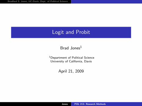
Logit Results from California Field Poll DataEstimate Std. Error z value Pr(>|z|)

(Intercept) 0.1620 0.3645 0.44 0.6568pid 0.3900 0.1453 2.68 0.0073

education −0.0367 0.0521 −0.71 0.4804income 0.1668 0.0905 1.84 0.0653latino 1.3348 0.3023 4.42 0.0000




I Signs? Related to log-odds ratios.

I Hypothesis testing: z-ratio is β̂/s.e.(β̂).

I 95 percent confidence interval approximately β̂ +−1.96(s.e.)

I Usual rules apply (and usual caveats).

I I advise against using stars. Why?

I Turn to interpretation



Interpreting the Model

I Consider probabilities first.

I Useful to compute tables of probabilities.

I e.g. what is Pr(y = 1 | profile)?I Non-latino, low-education, low-income, Republican?

I x1 = −1, x2 = 3, x3 = 1, x4 = 0

I Pr(y = 1 | Z ) = .46

I Same scenario, but for a Democrat?

I Pr(y = 1 | Z ) = .65

I Almost a .20 difference attributable to partisanship.

I But be careful.



Probabilities

I You can imagine there are a lot of probabilities you couldcompute.

I Specifically, 10 ∗ 5 ∗ 3 ∗ 2 = 300. Not all profiles exist, however!

I You could graph them as well. Consider income.

I Pr(y = 1) given a non-Latino Republican having mean-leveleducation.

I Let income assume each value and then plot it.





Probabilities

I You could overlay different probability scenarios on the graph.

I Marginal changes in Pr(y) are another way to interpret themodel.

I For logit:

∂ Pr(y = 1 | x)∂xk

=exp(xβ)

[1 + exp(xβ)]2βk

= Pr(y = 1 | x)[1− Pr(y = 1 | x)]βk (4)

I Analogy to regression: the marginal change is just β.

I Here, quantity of interest (probability) is nonlinear in x .

I Interpretation? It’s the slope of the probability curve holdingall other variables constant at some value.



Probabilities

I In probit, marginal change is given by:

∂ Pr(y = 1 | x)∂xk

= φ(xβ)βk (5)

I Same kind of interpretation is forthcoming from it.

I These are easy quantities to derive. If you use Stata, spostwill help you out here.

I But if we can compute probabilities (which we just have!), wecan compute marginal effects.

I Computing the marginal effects at means is sometimes useful.



Odds Ratios

I In logit, odds ratios may be useful.

I The odds ratio is just exp(β̂k).

I For a binary covariate, the interpretation is simple.

I Consider Latino origin variable. Coefficient is 1.335.

I Odds ratio? exp(1.335 ∗ 1) = 3.8.

I Interpretation: respondents of Latino origin are nearly 4 timesmore likely to claim support for temporary worker programthan when compared to non-Latino origin respondents.

I Nice interpretation.



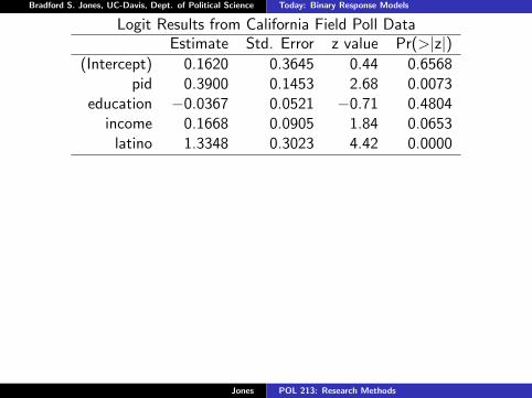
Odds Ratios

I Continuous variables

I Odds are proportional between adjacent categories.

I Percentage change in odds:

%∆pi

1− pi=

[exp(βk)x − exp(βk)x ′

exp(βk)x ′

]∗ 100 (6)

I For income covariate, the odds ratio when income=5 is: 2.3

I For income=4, odds ratio is: 1.9

I Change in odds of moving from category 4 to 5? About 18percent.

I For binary covariates, this is simple to compute.

I Odds for Latinos: 3.8; percentage change?

I (3.8− 1)/1=2.8 (or about 280 percent).



Probit

I Consider probit model on same data.

I Coefficients will be in “z-score” metric.

I Signage should be the same.

I As should significance.

I Only exceptions would be when extreme probabilities are ofinterest.



Probit Results from California Field Poll DataEstimate Std. Error z value Pr(>|z|)

(Intercept) 0.1358 0.2184 0.62 0.5340pid 0.2333 0.0871 2.68 0.0074

education −0.0239 0.0310 −0.77 0.4411income 0.0955 0.0540 1.77 0.0771latino 0.7629 0.1707 4.47 0.0000




I Signs? Related to z scores.

I Hypothesis testing: z-ratio is β̂/s.e.(β̂).

I 95 percent confidence interval approximately β̂ +−1.96(s.e.)

I Usual rules apply (and usual caveats).

I I advise against using stars. Why?

I Turn to interpretation.



Interpreting the Model

I Consider probabilities first.

I Useful to compute tables of probabilities.

I e.g. what is Pr(y = 1 | profile)?I Non-latino, low-education, low-income, Republican?

I x1 = −1, x2 = 3, x3 = 1, x4 = 0

I Pr(y = 1 | Z ) = .47 (z = −.074)

I Same scenario, but for a Democrat?

I Pr(y = 1 | Z ) = .65 (z = .39)

I Almost a .20 difference attributable to partisanship.

I But be careful.





Likelihood

I Assume binary response is Bernoulli distributed.I The PMF:

f (yi | xi ) = pyii (1− pi )

1−yi

I pi = F (x′iβ) (i.e. the probabilities assume some distributionfunction.)

I Since we like to work with log-likelihoods, the “generic”log-likelihood is:

logL(β) =N∑

i=1

{yi log F (x′iβ) + (1− yi ) log(1− F (x′iβ))}.

I MLE:

∂ logL∂β

=N∑

i=1

{yi

FiF ′i xi −

1− yi

1− FiF ′i xi

}= 0 (7)



Likelihood

I Often with binary response, we center on logit or probit.

I Log-likelihood redux:

logL(β) =N∑

i=1

{yi log p̂i + (1− yi ) log p̂i}.

I For logit, p̂i = Λ(x′i β̂Logit)

I For probit, p̂i = Φ(x′i β̂Probit)

I Λ and Φ were previously defined.



Likelihood

I First order conditions (logit):

N∑i=1

(yi − Λ(x′iβ))xi = 0

I First order conditions (probit):

N∑i=1

wi (yi − Φ(x′iβ))xi = 0

I wi is a weighting factor necessary for probit.



Next Time

I Interpretation and more on likelihood.

I Goodness-of-fit.


Documents

Binary data