Embed Size (px)
Citation preview

BIM-Based Data Mining Approach to Estimating Job Man-Hour Requirements in Structural Steel Fabrication
by
Xiaolin Hu
A thesis submitted in partial fulfillment of the requirements for the degree of
Master of Science
in
Construction Engineering and Management
Department of Civil and Environmental Engineering University of Alberta
© Xiaolin Hu, 2015

ii
ABSTRACT
In a steel fabrication shop, jobs from different clients and projects are
generally processed simultaneously in order to streamline production processes,
improve resource utilization, and achieve cost-effectiveness in serving multiple
concurrent steel-erection sites. Reliable quantity takeoff on each job and accurate
estimation of shop fabrication man-hour requirements are crucial to plan and
control fabrication operations and resource allocation on the shop floor. Building
information modeling (BIM) is intended to integrate multifaceted characteristics
of a building facility, but finds its application in structural steel fabrication largely
limited to design and drafting. This research focuses on extending BIM’s usage
further to the planning and control phases in steel fabrication. Using data
extracted from BIM-based models, a linear regression model is developed to
provide the man-hour requirement estimate for a particular job. Actual data
collected from a steel fabrication company was used to train and validate the
model. Two Excel macro-enabled workbooks were also developed to provide
decision-making support in fabrication planning.

iii
ACKNOWLEDGEMENTS
First of all, I would like to express my sincere thanks to my two academic
advisors, Dr. Ming Lu and Dr. Simaan M. AbouRizk for their vision, support, and
guidance in the preparation of this thesis.
Thanks are extended to Darrell Mykitiuk, Robert Wright, Jim Kanerva
and the staff at Waiward Steel Fabricators Ltd. (WSF) who shared their
knowledge and experience and provided data for this research. Their cooperation
and support are very much appreciated.
I am also grateful to all members at Construction Engineering and
Management group for their support and assistance during my graduate program.
Finally I would like to thank my family and my boyfriend, Sheng Mao, for
their continuous support and encouragement throughout my study at the
University of Alberta.

iv
The presented research is substantially funded by a National Science and
Engineering Council of Canada (NSERC) Collaborative Research and
Development Grant (CRDPJ 414616-11) and Waiward Steel Fabricators Ltd.
v
TABLE OF CONTENTS
CHAPTER 1. INTRODUCTION ................................................................................ 1
1.1 BACKGROUND.......................................................................................... 1
1.2 PROBLEM STATEMENT ............................................................................ 3
1.3 RESEARCH OBJECTIVES ...........................................................................5
1.4 METHODOLOGIES ................................................................................... 6
1.5 THESIS ORGANIZATION ........................................................................... 7
CHAPTER 2. BACKGROUND & LITERATURE REVIEW ............................................ 8
2.1 QUANTITY TAKEOFF ............................................................................... 8
2.2 STRUCTURAL STEEL FABRICATION ......................................................... 10
2.3 BUILDING INFORMATION MODELING (BIM) .......................................... 13
2.4 MACHINE LEARNING ............................................................................. 17
2.4.1 Machine Learning Algorithms ..................................................... 19
2.4.2 Linear Regression ........................................................................ 20
2.4.3 SVM Regression .......................................................................... 22
2.4.4 RBF Neural Network ................................................................... 25
2.4.5 Evaluation of Machine Learning Algorithms ............................... 27
2.4.6 Performance Measure ................................................................. 28
2.4.7 Applications in Construction ...................................................... 30
2.5 WEKA ................................................................................................. 32
CHAPTER 3. DATA PREPARATION ...................................................................... 35
3.1 DATA SOURCE ...................................................................................... 35
3.2 DATA SELECTION .................................................................................. 38
3.3 DATA PREPROCESSING .......................................................................... 40
3.3.1 Database Structure ...................................................................... 43
vi
3.4 DATA TRANSFORMATION ....................................................................... 51
CHAPTER 4. MODEL SELECTION & EVALUATION ............................................... 56
4.1 CANDIDATE MODELS ............................................................................ 56
4.2 CROSS VALIDATION ............................................................................... 57
4.3 EVALUATION ON TEST DATASET ............................................................ 63
CHAPTER 5. SHOP LOADING TOOLS ................................................................... 71
5.1 BACKGROUND........................................................................................ 71
5.2 SHOP LOADING TOOL ............................................................................ 72
5.2.1 Demonstration .............................................................................74
5.3 LOADING COMPARISON TOOL ................................................................ 75
5.3.1 Demonstration .............................................................................76
5.4 APPLICATION OF TOOLS ........................................................................ 78
CHAPTER 6. CONCLUSIONS ............................................................................... 80
6.1 SUMMARY ............................................................................................ 80
6.2 LIMITATIONS ......................................................................................... 81
6.3 RECOMMENDATIONS TO WSF ............................................................... 82
6.4 PROPOSAL FOR FUTURE RESEARCH....................................................... 83
REFERENCES .......................................................................................................... 84
APPENDIX A: SHOP LOADING TOOL MACRO CODE .................................................... 91
APPENDIX B: LOADING COMPARISON TOOL MACRO CODE ....................................... 98

vii
LIST OF TABLES
Table 2-1: Performance measures for numerical prediction (Witten, Frank, and
Hall 2011) .............................................................................................................. 29
Table 3-1: Material types and key attributes.......................................................... 51
Table 3-2: Sample data of a division ..................................................................... 54
Table 4-1: Evaluation comparison of various models ........................................... 60
Table 4-2: Information about variables in Equation (4-1) ................................... 63
Table 4-3: Evaluation summary of linear regression vs. experience .................... 69

viii
LIST OF FIGURES
Figure 1-1: Frame for productivity improvement (Dozzi and AbouRizk 1993) ...... 2
Figure 1-2: Hierarchy of a steel fabrication project ................................................ 4
Figure 2-1: Cost influence curve for project lifecycle (CII 1995) ............................ 8
Figure 2-2: An example of takeoff form .................................................................. 9
Figure 2-3: Steel fabrication processes .................................................................. 12
Figure 2-4: BIM workflow (Tekla 2014b) .............................................................. 14
Figure 2-5: A BIM example of steel structures (Tekla 2014b) ............................... 15
Figure 2-6: One-dimensional hyperplanes ........................................................... 22
Figure 2-7: Architecture of RBF network (Haykin 1999) ..................................... 26
Figure 2-8: WEKA GUI chooser ........................................................................... 33
Figure 3-1: An example of Tekla report (part-1) ................................................... 36
Figure 3-2: An example of Tekla report (part-2) ................................................... 37
Figure 3-3: An example of Tekla model ................................................................. 37
Figure 3-4: Labour tracking card (courtesy of WSF) ............................................ 39
Figure 3-5: Fabrication information structure in database .................................. 42
Figure 3-6: Part of the query result ...................................................................... 42
Figure 3-7: Database diagram – jobs and divisions ............................................. 45
Figure 3-8: Database diagram – schedule history ................................................ 46
Figure 3-9: Database diagram – employee timesheets .........................................47
Figure 3-10: Database diagram – fabrication drawings ....................................... 49
Figure 3-11: Database diagram – pieces and materials ........................................ 50
Figure 3-12: Formatted SQL data ......................................................................... 53
Figure 3-13: Data preparation framework ............................................................. 55
Figure 4-1: A perfect model................................................................................... 58
ix
Figure 4-2: Evaluation of RBF network using training set ................................... 59
Figure 4-3: Cross validation result of RBF network ............................................. 60
Figure 4-4: Cross validation result of SMO regression .......................................... 61
Figure 4-5: Cross validation result of linear regression ....................................... 62
Figure 4-6: Evaluation on independent test set ................................................... 65
Figure 4-7: Prediction results of test dataset .........................................................67
Figure 4-8: Prediction model sensitivity analysis ................................................ 68
Figure 5-1: Shop loading tool user interface .......................................................... 72
Figure 5-2: Workflow of generating shop loading chart ........................................ 73
Figure 5-3: Shop loading tool example ..................................................................74
Figure 5-4: Shop loading chart example ................................................................ 75
Figure 5-5: Loading comparison tool user interface..............................................76
Figure 5-6: Loading comparison tool example ...................................................... 77
Figure 5-7: Loading comparison chart example ................................................... 78
Figure 5-8: A proposed procedure for bid preparation .........................................79

1
Chapter 1. INTRODUCTION
1.1 BACKGROUND
Steel has long been the most important material to the construction sector
for its strength, durability, flexibility, efficiency, sustainability, and versatility
(SteelConstruction.info 2014). The production of steel pieces, which includes a
variety of operations of detailing, fitting, welding, and surface processing, is a
complex and critical process for a typical steel construction project. Most steel
construction projects use off-site structural steel fabrication shops to support the
erection sites in order to increase the productivity, gain better control over
quality, and reduce the total cost of projects (Eastman and Sacks 2008). A steel
fabrication shop usually makes use of shift work and serves multiple steel
erection sites at the same time to keep the business economical. Efficient
planning is substantial to steel fabrication to ensure a streamlined and delay-free
production process.
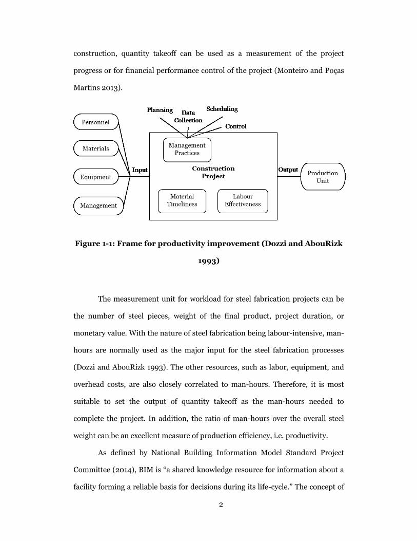
Figure 1-1 shows the structure of a typical construction project (Dozzi and
AbouRizk 1993). Personnel, materials, equipment, and management are
consumed by the system as resources to produce the construction units. As the
foundation of further planning and scheduling, estimating plays a critical role to
every construction project. Quantity takeoff is the most time-consuming yet
extremely important task in estimating. The following project scheduling and
control would benefit a great deal if quantity takeoff could be done accurately and
in a timely manner. For example, it can be used to foresee and plan the
construction activities during the pre-construction stage; in the process of
2
construction, quantity takeoff can be used as a measurement of the project
progress or for financial performance control of the project (Monteiro and Poças
Martins 2013).
Figure 1-1: Frame for productivity improvement (Dozzi and AbouRizk
1993)
The measurement unit for workload for steel fabrication projects can be
the number of steel pieces, weight of the final product, project duration, or
monetary value. With the nature of steel fabrication being labour-intensive, man-
hours are normally used as the major input for the steel fabrication processes
(Dozzi and AbouRizk 1993). The other resources, such as labor, equipment, and
overhead costs, are also closely correlated to man-hours. Therefore, it is most
suitable to set the output of quantity takeoff as the man-hours needed to
complete the project. In addition, the ratio of man-hours over the overall steel
weight can be an excellent measure of production efficiency, i.e. productivity.
As defined by National Building Information Model Standard Project
Committee (2014), BIM is “a shared knowledge resource for information about a
facility forming a reliable basis for decisions during its life-cycle.” The concept of

3
BIM has been rapidly gaining popularity and acceptance since Autodesk released
the BIM white paper (Autodesk 2003). Ideally, the vitality of a BIM-based model
spans the entire life-cycle of a project, from earliest conception to completion,
supporting processes like planning, design, cost control, construction
management, etc. This relatively new technology has also been adopted by the
steel fabrication industry, but only to find its use limited mostly to design and
drafting (Sattineni and Bradford 2011). Most of the advantages that BIM offers,
such as increased coordination of documents and effective information
communication and decision support for project management, are not exploited.
BIM-based models are utilized solely as 3D visualization in most cases. The
collaborating steel fabrication company for this research uses BIM software Tekla
to build 3D models for structural visualization, and generate 2D drawings for the
fabrication shop.
1.2 PROBLEM STATEMENT
A series of interviews with the estimators and project managers in the
steel fabrication industry reveal that the current estimating practice followed by
most steel fabricators is a manual process using spreadsheets and 2D drawings
generated by computer aided design (CAD) software or exported from BIM-based
models. Even with the availability of BIM, estimators use it as a visualization tool
to help them with reading the 2D drawings. Estimators use their experiences to
evaluate the project complexity and estimate the workload. The factor of human
interpretation in the process determines the error-proneness of the process.
The collaborating company is a leader in the steel fabrication and
construction services industries, offering services of procurement, engineering,
3D modeling, fabrication, coating, module assembly, erection, etc. Current
4
practice uses Tekla software (Tekla 2014a) to create 3D models from a customer’s
drawings, and further produce erection and fabrication drawings.
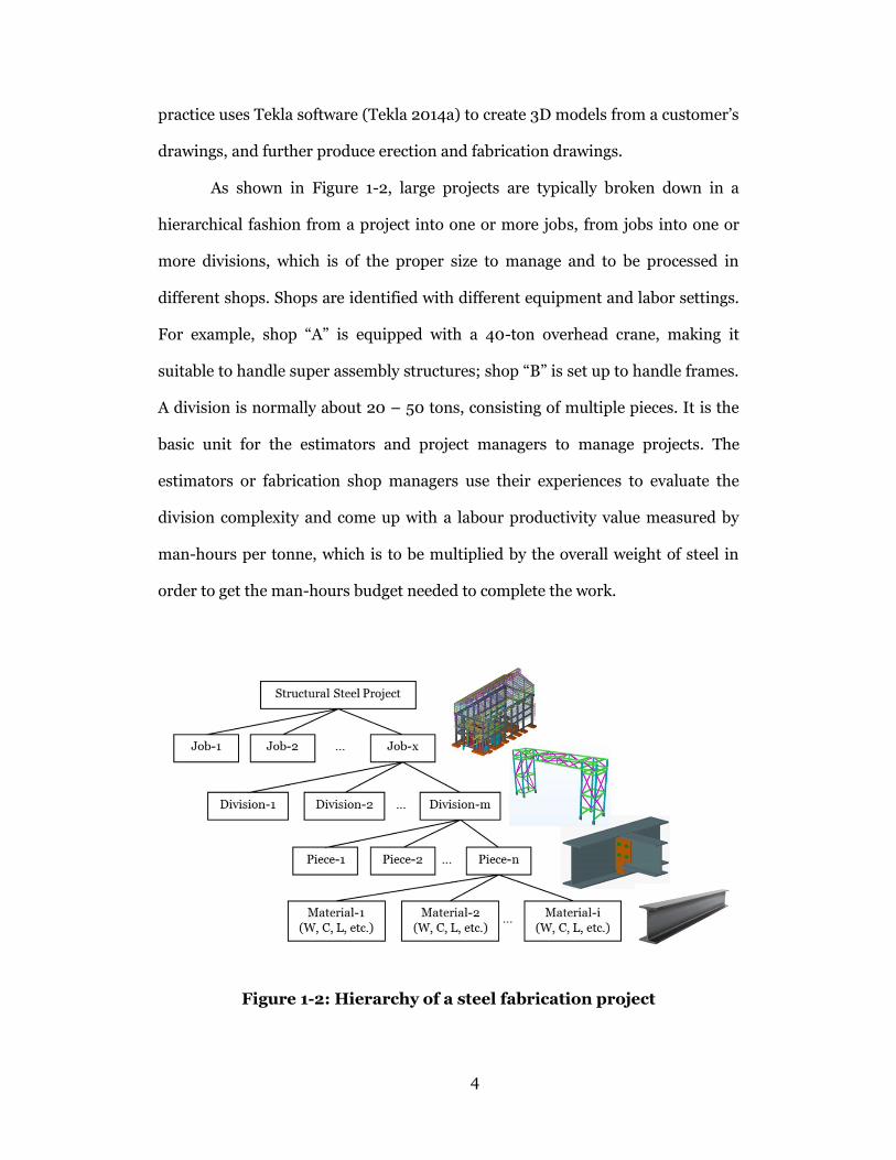
As shown in Figure 1-2, large projects are typically broken down in a
hierarchical fashion from a project into one or more jobs, from jobs into one or
more divisions, which is of the proper size to manage and to be processed in
different shops. Shops are identified with different equipment and labor settings.
For example, shop “A” is equipped with a 40-ton overhead crane, making it
suitable to handle super assembly structures; shop “B” is set up to handle frames.
A division is normally about 20 – 50 tons, consisting of multiple pieces. It is the
basic unit for the estimators and project managers to manage projects. The
estimators or fabrication shop managers use their experiences to evaluate the
division complexity and come up with a labour productivity value measured by
man-hours per tonne, which is to be multiplied by the overall weight of steel in
order to get the man-hours budget needed to complete the work.
Figure 1-2: Hierarchy of a steel fabrication project

5
The effectiveness of this practice depends to a great extent on personal
experience and knowledge, and may not always be consistent and reliable. The
abundant information contained in BIM, such as design details and predefined or
user-defined material properties, is not exploited properly.
Furthermore, job compositions of steel fabrication projects can vary
greatly from one to another. Even within the same job or division, the labour
requirements per unit weight of different material types are generally different.
For example, a piece demanding extensive welding obviously requires more man-
hours than a super-assembly connected by bolts.
1.3 RESEARCH OBJECTIVES
The objectives of the research presented in this thesis include:
Investigating the common applications of BIM in structural steel
fabrication;
Understanding the current estimating practices in steel fabrication
shops;
Exploring the possibility of extending BIM’s usage further to the
fabrication planning and control phase;
Providing decision support as to bid or not to bid after evaluating
the current and future workload;
Comparing three different modeling methods (linear regression,
SVM regression, and RBF neural network) to model steel
fabrication workload in terms of man-hours;
Providing a quantitative approach to the prediction of fabrication
man-hour requirements for structural steel projects by analyzing
and learning from the historical schedules and cost information

6
stored in the company’s central database for the benefits of
detailed estimating.
1.4 METHODOLOGIES
This study makes use of the material parts report generated from Tekla.
The essential attributes at the level of materials, as well as the summary level of
divisions, are collected and analyzed for 298 jobs and 1605 divisions completed
by the collaborating steel fabricator from 2009 to 2013. Only jobs that include
“supply work” are considered because erection is a process almost completely
separate from shop fabrication.
The first stage of this research is to design a meaningful data structure to
sort out and organize the data at different levels, and to collect necessary
information from the large database.
After historical data are collected, a regression model is developed. The
basic attributes of different material types are defined as independent input
variables. The man-hours needed to fabricate a division are defined as the output
variable. An open-source software, WEKA (Hall et al. 2009), is chosen to
complete the data mining task because of its wide collection of machine learning
algorithms and various regression functions. The selection of contributing factors
and the optimization of the variables through iterative experiments are all
facilitated by using WEKA. Different modeling methods are tested and compared
to find a suitable model for the workload of steel fabrication in terms of man-
hours.
At the third stage, the developed model is verified through an
independent dataset and the prediction results are compared with the forecast
made by personal judgment.

7
1.5 THESIS ORGANIZATION
The thesis starts with an introductory chapter that presents an overview of
the entire thesis, including the background, problem statement, research
objectives, and methodologies used.
Chapter 2 provides a thorough review of previous studies related to
construction estimating, data mining, application of regression analysis in the
construction field, and implementation of data mining algorithms.
Chapter 3 explains the raw data structure in detail and describes how the
data were prepared for modeling.
Chapter 4 presents the modeling process. A real case study from the
collaborating steel fabrication company is conducted as an example to illustrate
the validity, suitability and usefulness of the proposed method.
Chapter 5 demonstrates two automatic spreadsheet tools that can spread
the workload in the shop on a weekly basis in order to facilitate shop operation
planning.
Chapter 6 concludes the thesis with a summary of what has been achieved,
and outlines a proposal for future enhancements.
8
Chapter 2. BACKGROUND & LITERATURE REVIEW
2.1 QUANTITY TAKEOFF
Traditionally, a material takeoff (MTO) refers to the result or the process
of generating a list of required materials with quantities and other specifications
to accomplish a design by analyzing the drawings, blueprints, or other design
documents (Whitt 2012). Takeoff is followed by the estimating process, which is
to apply costs to the quantity measurements. Sometimes the terms quantity
takeoff and estimating may be used interchangeably if the desired results use the
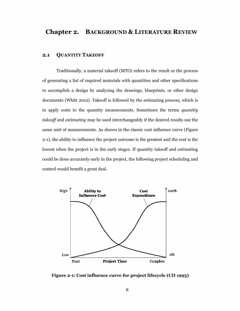
same unit of measurements. As shown in the classic cost influence curve (Figure
2-1), the ability to influence the project outcome is the greatest and the cost is the
lowest when the project is in the early stages. If quantity takeoff and estimating
could be done accurately early in the project, the following project scheduling and
control would benefit a great deal.
Figure 2-1: Cost influence curve for project lifecycle (CII 1995)

9
To perform quantity takeoff, several methods are available in the
construction industry. Traditional estimators do their takeoffs manually with
printed drawings. They would use colorful markers to keep track of different
materials and enter relevant information onto leger sheets or spreadsheets for
calculation. Figure 2-2 is a takeoff form template used by a company being
investigated during the present research. The quantity, unit weight, section detail,
etc. need be filled in manually for each line item. Some estimators adopt simple
annotation software to view electronic drawings and perform color-coding, etc.,
but the process is still manual in essence (Vertigraph Inc. 2004). Special
estimating software is another approach, but its input still relies heavily on
human interpretation.
Figure 2-2: An example of takeoff form
As stated by Tiwari et al. (2009), “Model-based cost estimating is the
process of integrating the object attributes from the 3D model of the designer
with the cost information from the database of the estimator.” Adopting BIM for

10
managing the design and construction process of projects has proven to be a
shared understanding (Aranda-Mena et al. 2009). BIM-based estimating would
assure the reduction of errors resulting from the repetitive manual entry of data,
allow high accuracy and standardisation in estimate production, which improves
estimators’ productivity. As commented by Monteiro and Poças Martins (2013),
BIM-based quantity takeoff is “one of the potentially most important and
profitable applications for BIM.” Yet, it is still generally underdeveloped and
underutilized.
2.2 STRUCTURAL STEEL FABRICATION
Steel is a widely used building material throughout the construction
industry because of its ability to suit different requirements of strength,
weldability, corrosion resistance, etc. (Williams 2011). It works like a skeleton to
hold the building structure up and together. When compared to other structural
building materials steel has a great many advantages. Unlike wood, steel does not
bend, twist, expand, or contract substantially because of the weather and
temperature. Unlike concrete, steel does not have a curing process and is at full
strength as soon as it is completed. Steel has more strength with less weight and
durability. Steel structures require little maintenance, do not age or decay as fast
as the other construction materials, and last longer (SteelConstruction.info 2014).
Steel construction is cost-efficient and can take place in most weather conditions.
Furthermore, steel is 100% recyclable and can be multi-cycled without losing
quality, making it one of the most environmentally friendly building materials.
There are generally a few stages in a typical steel construction project: design,
procurement, steel fabrication, shipment, optional module assembly, and on-site
erection, among which steel fabrication is a very critical part (Azimi et al. 2011).

11
Fabrication is defined by Berman (2014) as “the act of changing steel from
the mill or warehouse into the exact configuration needed for assembly into a
shipping piece or directly into a structural frame.” It mostly takes place in an
offsite fabrication shop that is highly regulated, controlled, confined, safe, and
equipped with leading edge specialized fabrication systems. All structural steel
components, such as columns, beams, channels, and plates, can be carefully
designed and precisely fabricated before delivery to site to be assembled and
erected.
The systematic fabrication process generally consists of a series of
operations including cutting, grinding, drilling, burning, fitting, welding, and
surface processing (painting, sand blasting, fireproofing etc.). The whole shop
floor is divided into several main areas according to the specific functions, and
each shop (for instance, cutting shop, fitting shop, welding shop, and painting
shop) is equipped with specialized machines, tools, and skilled personnel. The
inputs of a steel fabrication shop are raw steel materials and shop fabrication
drawings, and the outputs are fabricated steel components that are ready to be
assembled and shipped to site for erection (Figure 2-3).
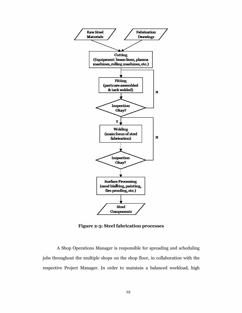
12
Figure 2-3: Steel fabrication processes
A Shop Operations Manager is responsible for spreading and scheduling
jobs throughout the multiple shops on the shop floor, in collaboration with the
respective Project Manager. In order to maintain a balanced workload, high

13
production rate, and streamlined operations, the manager needs to define the
scope of a job well in terms of man-hours, which is what this study focuses on.
2.3 BUILDING INFORMATION MODELING (BIM)
According to the National Building Information Model Standard Project
Committee (2014),
Building Information Modeling (BIM) is a digital representation of
physical and functional characteristics of a facility. A BIM is a shared
knowledge resource for information about a facility forming a reliable
basis for decisions during its life-cycle; defined as existing from earliest
conception to demolition.
A basic premise of BIM is collaboration by different stakeholders at
different phases of the life cycle of a facility to insert, extract, update or
modify information in the BIM to support and reflect the roles of that
stakeholder.
The US National BIM Standard will promote the business requirements
that BIM and BIM interchanges are based on:
a shared digital representation,
that the information contained in the model be interoperable (i.e.:
allow computer to computer exchanges), and
the exchange be based on open standards,
the requirements for exchange must be capable of defining in
contract language.

14
The concept of BIM has been rapidly gaining popularity and acceptance
since Autodesk released the BIM white paper (Autodesk 2003). Ideally, the
vitality of a BIM-based model spans the entire life-cycle of a project, from earliest
conception to completion, supporting processes like planning, design, cost
control, construction management etc. BIM solutions can be customised and
applied to various areas, for instance, concrete construction, steel fabrication,
steel erection, rebar fabrication, and structural design. Figure 2-4 (Tekla 2014b)
shows the workflow and the integration of all the services in steel fabrication
industry. Ideally, the bidding, preconstruction, construction, and post
construction of a project can all be managed through BIM as a whole instead of
jumping across multiple software and systems, avoiding having to deal with
abundant document format transformations. It is a platform to share knowledge
among different project stakeholders, providing consistent and coordinated
representations of the digital model.
Figure 2-4: BIM workflow (Tekla 2014b)

15
Figure 2-5 (Tekla 2014b) shows a portion of a BIM-based model, along
with a view of the component coding system the model uses. It represents a steel
structure that consists of beams, columns, handrails, and is connected with bolts.
Figure 2-5: A BIM example of steel structures (Tekla 2014b)
To seize the full potential value of BIM, contractors cannot limit their
exploration of BIM to 3D modeling and visualization only. 3D rendering is the
basic use of BIM. BIM can also be used to detect clashes and conflicts. Detailed
fabrication drawings can be generated for different trades. Change orders and
addendums can easily be communicated between different parties. 3D models
combined with other planning techniques and tools can provide powerful
construction monitoring, which in turn helps with scheduling and updating 3D
models (Hergunsel 2011).
The Industry Foundation Classes (IFC) data model is “a platform neutral,
open file format specification” intended to provide a set of consistent data
representations of building and construction industry information (Eastman

16
2006). It is developed by buildingSMART to facilitate interoperability in the
Architecture, Engineering, and Construction (AEC) industry. Add-ons and
extensions can be developed using IFC format to facilitate the communication
between different BIM-related systems.
Significant research has been carried out in exploration of BIM. The study
conducted by Howard and Björk (2008) is an overview of experts’ views on BIM.
It collects some pilot use cases and BIM user experience from a number of
leading property owners in spite of the complexity of the formal standards such
as the IFCs. Aranda-Mena et al. (2009) provided insights into BIM and
illustrated its importance and potential applications in construction project
management industry through case studies. Steel, Drogemuller, and Toth (2012)
presented their experience with model-based interoperability issues, successes,
and challenges in BIM exchange between various tools; a business case
framework to facilitate the adoption of BIM was proposed. Jung and Joo (2011)
developed a comprehensive BIM framework consisting of three dimensions and
six categories, which provides a basis for the evaluation of practical BIM
effectiveness. Nawari (2012) reviewed the importance of BIM standards in off-
site construction and its role in data exchange. An Information Delivery Manual
(IDM) was also proposed, which provides material description of building
construction processes, information requirements, and expected process outputs
in the study. Furthermore, BIM can provide support to teaching construction
project management (Peterson et al. 2011). The introduction of BIM-based
project management tools helped educators design more realistic project-based
assignments and cases, and supported students with learning the integration and
application of different project management functions.

17
Ikerd (2008) justified the importance of BIM in structural engineering.
Shi (2009) proposed a framework of integrating Radio Frequency Identification
(RFID) with BIM technologies for the decision-making processes in structural
steel fabrication and erection. A portable RFID database scheme was developed
to increase the efficiency and accuracy in steel fabrication and erection. Xie, Shi,
and Issa (2010) further discussed the BIM/RFID implementation in computer-
aided design, manufacturing, engineering, and installation processes. Tiwari et al.
(2009) applied BIM tools for Target Value Design (TVD) on a large healthcare
project in Northern California. A 4D simulation for a steel arch bridge was
produced to illustrate the use of BIM tools in a design review and lifting plan
study (Chiu et al. 2011). Lancaster and Tobin (2013) outlined their firms’
extensive experience with BIM, providing strategies and new understandings of
applying BIM to structural engineering projects aimed to accommodate
Integrated Project Delivery (IPD). Kalavagunta (2012) presented an integrated
structural modeling workflow for structural design. Sattineni and Bradford (2011)
conducted a survey of construction practitioners in United States to determine
the usage of BIM in various tasks, especially in construction cost estimating.
Monteiro and Poças Martins (2013) also explored automatic BIM based quantity
takeoff and a case study was presented. As one of its conclusions, the authors
suggested that takeoff specifications such as manual measurements should be
revised to account for BIM features in order to minimize the limitations in
current practice.
2.4 MACHINE LEARNING
People have been looking for information in the sea of data ever since
human beings became intelligent, and the identification of potentially useful

18
information or patterns hidden in the huge amount of data around us is what
experience, knowledge, and intelligence are actually about. Machine learning, as
a branch of artificial intelligence (AI), is about the study and construction of
systems, other than human brains, that can solve problems by analyzing and
learning from data. In 1959, Arthur Samuel defined machine learning as “a field
of study that gives computers the ability to learn without being explicitly
programmed” (Simon 2013). It provides tools to make predictions automatically
or help people make decisions about complex and scaled problems from data in a
faster and more accurate way. A more formal and widely quoted definition of
machine learning is provided by Mitchell (1997):
A computer program is said to learn from experience E with respect to
some class of tasks T and performance measure P, if its performance at
tasks in T, as measured by P, improves with experience E.
This fundamentally operational definition makes it clear that the class of
tasks, the source of experience, and the measure of performance to be improved
are the three features that have to be identified in order to have a well-defined
learning problem (Mitchell 1997).
The term machine learning is commonly confused with data mining.
These two areas overlap significantly in the methods they employ, focusing on
slightly different goals. As mentioned before, machine learning relates to the
study and development of learning algorithms and focuses on prediction in most
cases. Data mining, on the other hand, can be defined as the process of trying to
extract previously unknown knowledge, properties, or patterns from
unstructured data. It focuses on the discovery aspect. Data mining may utilize

19
machine learning algorithms during the process, and may also drive the
advancement of machine learning techniques (Cross Validated 2013;
ResearchGate 2013).
2.4.1 Machine Learning Algorithms
A popular taxonomy of organizing machine learning algorithms is based
on the learning styles algorithms can adopt (Brownlee 2013a):
Supervised Learning: Algorithms are trained on input data that
have a known label or desired result, such as sunny/rainy or
spam/not-spam. Such an algorithm attempts to create a model to
make predictions of the outputs according to the inputs. The
model is like a function or mapping from the inputs to outputs.
Once a desired level of accuracy is achieved (i.e. the predictions
and the labels are close enough), the trained model is able to
generate outputs for inputs that have not been used in the training
process. Classification and regression problems fall into this
category. Example algorithms are Decision Trees, Stepwise
Regression and Back-Propagation Neural Networks.
Unsupervised Learning: Training examples are not labelled and do
not have a known result. Instead of generalising a function or
mapping from inputs to outputs, a model is prepared by
discovering structures present in the input data. Example
algorithms are K-Means Clustering and Apriori Algorithm.
Semi-Supervised Learning: Input data consist of both labelled and
unlabelled examples. The desired model needs to be able to make
predictions as well as deducing the structures in the data. An

20
example problem would be image classification where only few
examples are labelled in a large dataset.
Reinforcement Learning: Input data are provided as stimulus. A
model attempts to gather knowledge in an environment through
punishment or reward feedbacks about its actions. The goal is to
maximize some cumulative reward. Example algorithms are Q-
Learning and Temporal Difference Learning. This type of learning
is more likely to be used in certain kinds of control system
development.
Another grouping method is by algorithm similarity. For example,
regression methods, decision tree methods, instance-based methods, associate
rule learning, clustering methods, and artificial neural networks. In the following
section, only the basic linear regression algorithm is introduced as it is the
method used in this research.
2.4.2 Linear Regression
Linear regression is actually a fundamental method in statistics, suitable
for situations where most or all the attributes are numeric. The basic idea is to
express the model as a linear mapping from the attributes to the output class. The
goal is to come up with “a function that approximates the training points well by
minimizing the prediction error” (Witten, Frank, and Hall 2011). A model is
represented as:
𝑥 = 𝑤0 + 𝑤1𝑎1 + 𝑤2𝑎2 + ⋯ + 𝑤𝑘𝑎𝑘 (2-1)
where 𝑥 is the outcome or class; 𝑎1, 𝑎2, … , 𝑎𝑘 are the numeric attribute
values; and 𝑤0, 𝑤1, 𝑤2, … , 𝑤𝑘 are weights for each attribute.

21
The weights are calculated from the training data. Each training instance
has its own set of attribute values 𝑎1(𝑖), 𝑎2
(𝑖), … , 𝑎𝑘(𝑖) and the outcome 𝑥(𝑖) .
Assuming an extra attribute 𝑎0 with a constant value of 1, then the predicted
value for the class can be conveniently written as:
𝑤0𝑎0(𝑖) + 𝑤1𝑎1
(𝑖) + 𝑤2𝑎2(𝑖) + ⋯ + 𝑤𝑘𝑎𝑘
(𝑖) = ∑ 𝑤𝑗𝑎𝑗(𝑖)𝑘
𝑗=0 (2-2)
The method of linear regression is to look for a set of numeric weights
𝑤0, 𝑤1, 𝑤2, … , 𝑤𝑘 to make the predicted values as close to the actual values as
possible; in other words, to minimize the sum of the squares of the differences
over all the training instances (Witten, Frank, and Hall 2011). In order to choose
coefficients properly, the function shown in (2-3) is the target to be minimized.
This is the classic least-squares linear regression method.
∑ (𝑥(𝑖) − ∑ 𝑤𝑗𝑎𝑗(𝑖)𝑘
𝑗=0 )2𝑛
𝑖=1 (2-3)
Once a set of numeric weights has been calculated based on the training
data, the prediction of the outcome of new instances can be accomplished using
the formula.
Aside from the complete numeric cases, linear regression is able to handle
nominal attributes as well. In contrast to the continuous nature of numeric
attributes that measure real or integer numbers, nominal attributes handle a pre-
defined set of values and are sometimes called categorical attributes. The finite
set of values serve only as names or symbols (Witten, Frank, and Hall 2011). The
trick of applying linear regression to nominal attributes is to view each possible
value of the nominal attributes as a binary attribute, whose value is either 0 or 1.
There are more advanced variations of the standard linear regression, such as
logistic regression and multivariate linear regression, which is not covered in this
research.
22
2.4.3 SVM Regression
Support Vector Machines (SVMs) are supervised learning models with
associated learning algorithms, belonging to a family of generalized linear
classifiers. The current standard “soft margin” method was proposed by Cortes
and Vapnik (1995) on the basis of the original algorithm invented by Vladimir N.
Vapnik in 1979. SVM can be applied not only to classification problems but also
to regression analysis for its ability of analyzing data and recognizing patterns.
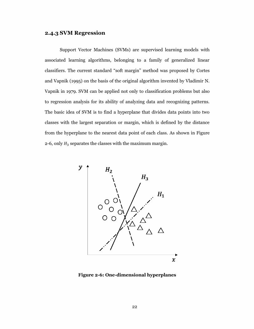
The basic idea of SVM is to find a hyperplane that divides data points into two
classes with the largest separation or margin, which is defined by the distance
from the hyperplane to the nearest data point of each class. As shown in Figure
2-6, only 𝐻3 separates the classes with the maximum margin.
Figure 2-6: One-dimensional hyperplanes
23
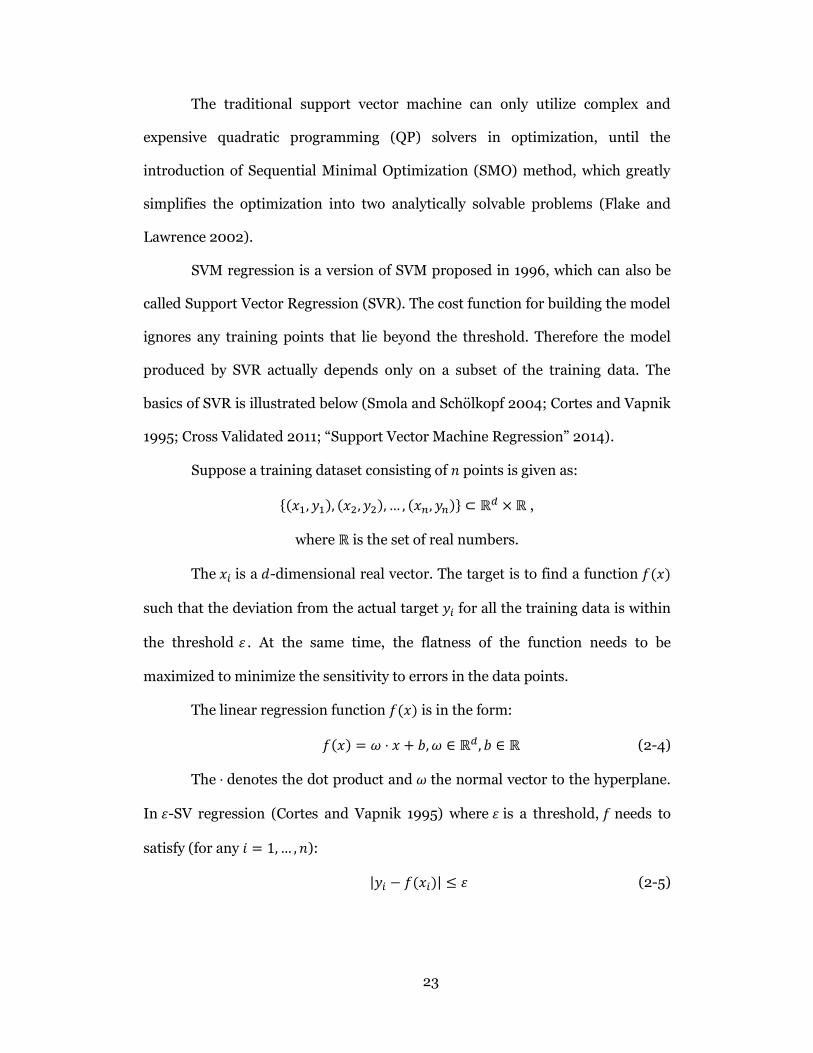
The traditional support vector machine can only utilize complex and
expensive quadratic programming (QP) solvers in optimization, until the
introduction of Sequential Minimal Optimization (SMO) method, which greatly
simplifies the optimization into two analytically solvable problems (Flake and
Lawrence 2002).
SVM regression is a version of SVM proposed in 1996, which can also be
called Support Vector Regression (SVR). The cost function for building the model
ignores any training points that lie beyond the threshold. Therefore the model
produced by SVR actually depends only on a subset of the training data. The
basics of SVR is illustrated below (Smola and Schölkopf 2004; Cortes and Vapnik
1995; Cross Validated 2011; “Support Vector Machine Regression” 2014).
Suppose a training dataset consisting of 𝑛 points is given as:
{(𝑥1, 𝑦1), (𝑥2, 𝑦2), … , (𝑥𝑛 , 𝑦𝑛)} ⊂ ℝ𝑑 × ℝ ,
where ℝ is the set of real numbers.
The 𝑥𝑖 is a 𝑑-dimensional real vector. The target is to find a function 𝑓(𝑥)
such that the deviation from the actual target 𝑦𝑖 for all the training data is within
the threshold 휀 . At the same time, the flatness of the function needs to be
maximized to minimize the sensitivity to errors in the data points.
The linear regression function 𝑓(𝑥) is in the form:
𝑓(𝑥) = 𝜔 ⋅ 𝑥 + 𝑏, 𝜔 ∈ ℝ𝑑, 𝑏 ∈ ℝ (2-4)
The ⋅ denotes the dot product and 𝜔 the normal vector to the hyperplane.
In 휀-SV regression (Cortes and Vapnik 1995) where 휀 is a threshold, 𝑓 needs to
satisfy (for any 𝑖 = 1, … , 𝑛):
|𝑦𝑖 − 𝑓(𝑥𝑖)| ≤ 휀 (2-5)
24
And maximization of the flatness of the function in (2-4) can be achieved
by minimizing the norm of 𝜔, i.e. ‖𝜔‖. Consequently the objective is to solve the
following optimization problem (Smola and Schölkopf 2004):
minimize ‖𝜔‖
subject to {
𝑦𝑖 − 𝜔 ⋅ 𝑥𝑖 − 𝑏 ≤ 휀
𝜔 ⋅ 𝑥𝑖 + 𝑏 − 𝑦𝑖 ≤ 휀 (2-6)
However, a function 𝑓 that satisfies all pairs (𝑥𝑖 , 𝑦𝑖) with 휀 precision may
not actually exist. Moreover some errors also need to be allowed for. Accordingly
the infeasible constraints of the optimization problem (2-6) are loosened by
introducing non-negative slack variables 𝜉𝑖+, 𝜉𝑖
− that are used in the “soft margin”
cost function in SVM. Hence the optimization problem is transformed to (Smola
and Schölkopf 2004):
minimize 1
2‖𝜔‖2 + 𝐶 ∑ (𝜉𝑖
+ + 𝜉𝑖−)𝑛
𝑖=1 , (𝐶 is a positive constant)
subject to {
𝑦𝑖 − 𝜔 ⋅ 𝑥𝑖 − 𝑏 ≤ 휀 + 𝜉𝑖+
𝜔 ⋅ 𝑥𝑖 + 𝑏 − 𝑦𝑖 ≤ 휀 + 𝜉𝑖−
𝜉𝑖+, 𝜉𝑖
− ≥ 0
(2-7)
The solution to the problem above is to construct a Lagrange function
from the objective function as (Smola and Schölkopf 2004):
𝐿 ≜1
2‖𝜔‖2 + 𝐶 ∑(𝜉𝑖
+ + 𝜉𝑖−)
𝑛
𝑖=1
− ∑(𝛼𝑖𝜉𝑖+ + 𝛽𝑖𝜉𝑖
−)
𝑛
𝑖=1
− ∑ 𝛾𝑖(휀 + 𝜉𝑖+ − 𝑦𝑖 + 𝜔 ⋅ 𝑥𝑖 + 𝑏)
𝑛
𝑖=1
− ∑ 𝛿𝑖(휀 + 𝜉𝑖− + 𝑦𝑖 − 𝜔 ⋅ 𝑥𝑖 − 𝑏)𝑛
𝑖=1 (2-8)
𝐿 is the Lagrangian and 𝛼𝑖, 𝛽𝑖 , 𝛾𝑖, 𝛿𝑖 are Lagrange multipliers. Having
derived the Lagrange function, the Support Vector expansion is conducted as
(Smola and Schölkopf 2004):
𝜔 = ∑ (𝛾𝑖 − 𝛿𝑖)𝑥𝑖𝑛𝑖=1 (2-9)
Hence:

25
𝑓(𝑥) = ∑ (𝛾𝑖 − 𝛿𝑖)(𝑥𝑖 ⋅ 𝑥)𝑛𝑖=1 + 𝑏 (2-10)
According to (2-9), 𝜔 can be completely calculated by the linear
combination of the training data points 𝑥𝑖.
The constant offset 𝑏 can be computed via various methods such as
exploiting the Karush-Kuhn-Tucker (KKT) conditions and as a by-product of the
optimization process (Smola and Schölkopf 2004).
2.4.4 RBF Neural Network
A radial basis function (RBF) neural network is an artificial neural
network widely used for functional approximation and prediction in areas such as
time-series modeling, system control and pattern classification. The name comes
from its use of radial basis functions as activation functions (Broomhead and
Lowe 1988).
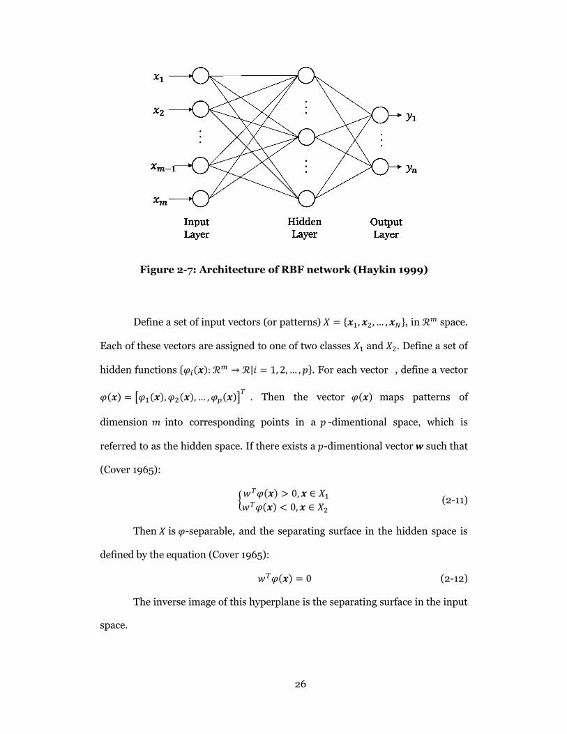
In a RBF network there are basically three layers with different roles as
shown in Figure 2-7: an input layer, a hidden layer and an output layer. The first
layer is simply a fan-out layer, acting as a connection between the network and
the environment. No processing is done. The second layer, i.e. the hidden layer,
transforms the nonlinear input space to the hidden space, which in most cases is
higher dimensional. The last one, output layer, applies a linear transformation
(Haykin 1999). The rationale is justified by Cover’s theorem on the separability of
patterns (Cover 1965). By using a nonlinear mapping to transform the input
space in a higher dimensional space, the complex patterns can be more linearly
separable. The nonlinear mapping is then followed by a linear mapping from the
hidden space to the output space.
26
Figure 2-7: Architecture of RBF network (Haykin 1999)
Define a set of input vectors (or patterns) 𝑋 = {𝒙1, 𝒙2, … , 𝒙𝑁}, in ℛ𝑚 space.
Each of these vectors are assigned to one of two classes 𝑋1 and 𝑋2. Define a set of
hidden functions {𝜑𝑖(𝒙): ℛ𝑚 → ℛ|𝑖 = 1, 2, … , 𝑝}. For each vector , define a vector
𝜑(𝒙) = [𝜑1(𝒙), 𝜑2(𝒙), … , 𝜑𝑝(𝒙)]𝑇
. Then the vector 𝜑(𝒙) maps patterns of
dimension 𝑚 into corresponding points in a 𝑝 -dimentional space, which is
referred to as the hidden space. If there exists a 𝑝-dimentional vector 𝒘 such that
(Cover 1965):
{𝑤𝑇𝜑(𝒙) > 0, 𝒙 ∈ 𝑋1
𝑤𝑇𝜑(𝒙) < 0, 𝒙 ∈ 𝑋2 (2-11)
Then 𝑋 is 𝜑-separable, and the separating surface in the hidden space is
defined by the equation (Cover 1965):
𝑤𝑇𝜑(𝒙) = 0 (2-12)
The inverse image of this hyperplane is the separating surface in the input
space.

27
Given data pairs (𝒙𝟏, 𝑑1), (𝒙𝟐, 𝑑2), … (𝒙𝑵, 𝑑𝑁) ∈ ℛ𝑚 × ℛ, the interpolation
problem is to find a function 𝐹: ℛ𝑚 → ℛ that satisfies the interpolation condition:
𝐹(𝒙𝑖) = 𝑑𝑖, 𝑖 = 1, 2, … , 𝑁 (2-13)
The RBF technique is to choose a function 𝐹 in the form (Haykin 1999):
𝐹(𝒙) = ∑ 𝑤𝑖𝜑(‖𝒙 − 𝒙𝒊‖)𝑁𝑖=1 (2-14)
where 𝑤𝑖 ∈ ℛ are weight factors.‖∙‖ denotes a norm between 𝒙 and 𝒙𝒊 ,
which is usually Euclidean distance. {𝜑(‖𝒙 − 𝒙𝒊‖)|𝑖 = 1, 2, … , 𝑁} is a set of radial
basis functions, the value of which depends solely on the distance from the data
point to the origin. Gaussian function is one of the popular choice and is in the
following form:
𝜑(𝑟) = 𝑒−
𝑟2
2𝜎2 (2-15)
where 𝜎 defines the width of the bell-shape.
When choosing the center nodes of the RBF network in the hidden layer,
aside from using K-means clustering, the centers can also be randomly sampled
from the dataset. This step is unsupervised. If the RBF network is used for
pattern classification, a hard-limiter or sigmoid function could be placed on the
output neurons to generate categorical values.
2.4.5 Evaluation of Machine Learning Algorithms
Having defined the problem and prepared the data, machine learning
algorithms will be applied to the data to solve the problem. Multiple tests are
needed to run and tune the algorithms in order to discover whether there is a
pattern or structure in the problem for the algorithm to learn, and decide which
algorithms are effective for the problem.
28
The step before applying any algorithm is to prepare a training dataset
and a test dataset out of the transformed dataset. The two datasets need to be
representative of the problem. Generally the intersection of the two sets is empty,
meaning that the training dataset and the test dataset are independent of one
another. An algorithm will be trained on the training dataset and evaluated
against the test dataset.
Other than using separate training and test datasets, another approach is
to use the whole transformed dataset to train and test an algorithm, which is
called cross validation. The first step of N-fold cross validation method is to
separate the dataset into N groups of instances of the equal size M. Each group is
called a fold. The model is trained on N-1 folds and then tested on the one fold
that was left out. The process is repeated so that each of the N fold is left out and
act as a test dataset. In the end, the average of the performance measures of the N
folds is used to evaluate the performance of the algorithm on the problem. This
method resolves the balance issue between the size and representation of training
and test datasets. It is often used when the transformed dataset is not large
enough to be split into a training and a test datasets of suitable size.
2.4.6 Performance Measure
The performance measure is the measurement of the performance or
quality of solutions to a problem. It is the way to evaluate the success of different
machine learning experiments. For numerical prediction, a few measures to
interpret the performance of the predictions made by a trained model on the test
dataset are listed in Table 2-1. Assume the actual values of the test instances are
𝑎1, 𝑎2, … , 𝑎𝑛; the predicted values calculated by the model are 𝑝1, 𝑝2, … , 𝑝𝑛; 𝑛 is the
total number of test instances; �̂� is the average value from the training dataset; 𝑎
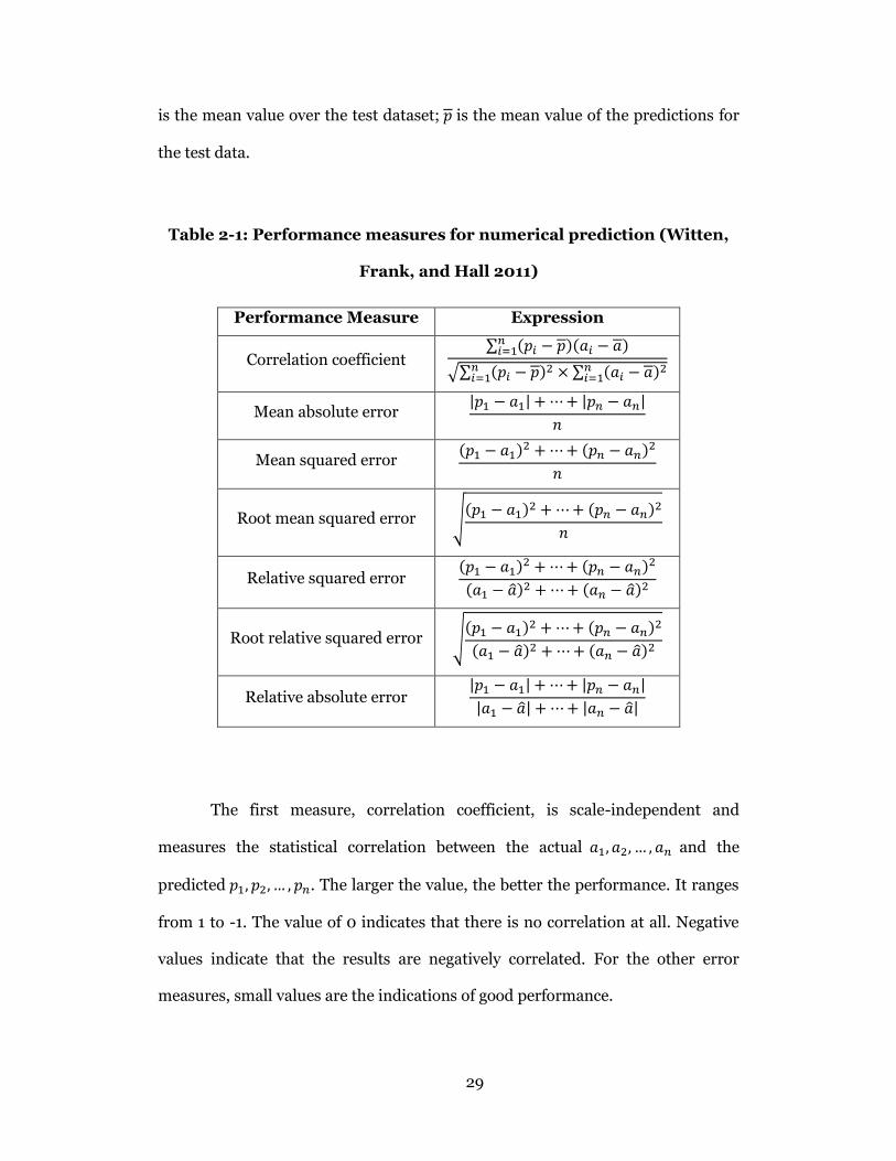
29
is the mean value over the test dataset; 𝑝 is the mean value of the predictions for
the test data.
Table 2-1: Performance measures for numerical prediction (Witten,
Frank, and Hall 2011)
Performance Measure Expression
Correlation coefficient ∑ (𝑝𝑖 − 𝑝)(𝑎𝑖 − 𝑎)𝑛
𝑖=1
√∑ (𝑝𝑖 − 𝑝)2𝑛𝑖=1 × ∑ (𝑎𝑖 − 𝑎)2𝑛
𝑖=1
Mean absolute error |𝑝1 − 𝑎1| + ⋯ + |𝑝𝑛 − 𝑎𝑛|
𝑛
Mean squared error (𝑝1 − 𝑎1)2 + ⋯ + (𝑝𝑛 − 𝑎𝑛)2
𝑛
Root mean squared error √(𝑝1 − 𝑎1)2 + ⋯ + (𝑝𝑛 − 𝑎𝑛)2
𝑛
Relative squared error (𝑝1 − 𝑎1)2 + ⋯ + (𝑝𝑛 − 𝑎𝑛)2
(𝑎1 − �̂�)2 + ⋯ + (𝑎𝑛 − �̂�)2
Root relative squared error √(𝑝1 − 𝑎1)2 + ⋯ + (𝑝𝑛 − 𝑎𝑛)2
(𝑎1 − �̂�)2 + ⋯ + (𝑎𝑛 − �̂�)2
Relative absolute error |𝑝1 − 𝑎1| + ⋯ + |𝑝𝑛 − 𝑎𝑛|
|𝑎1 − �̂�| + ⋯ + |𝑎𝑛 − �̂�|
The first measure, correlation coefficient, is scale-independent and
measures the statistical correlation between the actual 𝑎1, 𝑎2, … , 𝑎𝑛 and the
predicted 𝑝1, 𝑝2, … , 𝑝𝑛. The larger the value, the better the performance. It ranges
from 1 to -1. The value of 0 indicates that there is no correlation at all. Negative
values indicate that the results are negatively correlated. For the other error
measures, small values are the indications of good performance.

30
The appropriate choice of performance measures requires considerations
of the specific problem and application. For example, the squared error measures
and root squared error measures tend to amplify the large discrepancies of
prediction errors, whereas the absolute error measures do not have this effect.
Fortunately, all the performance measures are easy to calculate. In most
situations, the measured results of a numerical prediction method is consistent
no matter which mathematical performance measure is used.
2.4.7 Applications in Construction
Artificial intelligence has long been adopted by researchers for modeling
and solving problems in the construction industry. Modeling techniques such as
artificial neural network (ANN), regression models, and decision trees have been
introduced to study the relationships between all kinds of factors in construction
processes using historical data.
Song and AbouRizk (2008) used ANN to model the relationship of
influencing factors and steel drafting and fabrication productivities. They
proposed a systematic approach to make use of historical data, and applied the
methodology to measuring and modeling steel drafting and fabrication tasks.
Portas (1996) developed a back-propagation, feed-forward neural network system
to provide support in the labor productivity estimation for concrete formwork.
The inputs to the system are contributing factors to labour productivity, and the
output is a set of binary scores representing certainty of occurrence in
correspondence with the subset ranges of productivity values that can be used to
predict performance of the labour productivity of future projects. ANN has also
been used to model the relationship between influencing factors and construction
productivity in trades like earthmoving equipment productivity (Karshenas and
31
Feng 1992), concrete construction productivity (Sonmez and Rowings 1998), and
productivity of spool fabrication in the shop and pipe installation in the field (Lu
2001). These researches all proved the effectiveness of ANN in addressing the
complexity in construction productivity modeling. At the preparation step,
various methods of data collection and productivity measurement were also
explored in different trades. Furthermore, instead of utilizing an existing ANN
scheme, Lu (2001) developed a new ANN scheme, combining classification and
prediction on the basis of Kohonen’s LVQ concept and with a probabilistic
method integrated, to suit the requirements in the problem domain. It is named
the Probability Inference Neural Network (PINN). The new model was applied to
predict labour production rates and was proven effective in solving high
dimensional mapping of input and output with multiple influential factors.
Hu and Mohamed (2012) explored two different techniques, artificial
intelligence planning and dynamic programming, to solve the automation
problem in sequencing decision making in construction. More specifically, they
applied Planning Domain Description Language (PDDL), which is a domain-
independent artificial intelligence planning language.
Fayek and Oduba (2005) used fuzzy logic expert systems to predict
productivity of pipe rigging and welding. Contributing factors that affect the
productivity of each activity were identified. Fuzzy membership functions and
expert rules were developed. Actual data collected from a construction project
were used to validate the models, which were proved to have high accuracy of
linguistic prediction.
Smith (1999) applied multiple regression-based models to study
earthmoving productivity with focus on investigation of the relationships between
earthmoving operating conditions and productivity and bunching. The models
32
developed suggested a strong linear relationship between the operating
conditions and productivity. Lee et al. (2013) used regression analysis to develop
a quantity prediction model for reinforced concrete and bricks in education
facilities that were built as a result of the Build-Transfer-Lease (BTL) projects
actively promoted by the Korean government. Linear regression is also used to
develop condition prediction models of oil and gas pipelines in order to provide
decision support to practitioners in planning for pipeline maintenance (El-
Abbasy et al. 2014). Linear regression was explored to suit the numerical output
type of the proposed pipeline condition assessment models. The influential
factors that have a major impact on pipeline conditions were selected by
presenting a questionnaire to experts and reviewing literature. Five condition
prediction models were developed and a sensitivity analysis was conducted to
learn about the impact degree of each factor on the model output individually.
2.5 WEKA
WEKA is an open source data mining software written in Java developed
by the machine learning group at the University of Waikato, New Zealand. It is a
modern platform and workbench for applied machine learning. The name WEKA
is an acronym which stands for Waikato Environment for Knowledge Analysis.
Incorporated into WEKA is a comprehensive collection of machine learning
techniques and algorithms that can be applied directly to a dataset. Also included
are tools for data pre-processing, classification, regression, clustering, association
rules, evaluation methods, and functions that are suited for the development of
new machine learning schemes (The University of Waikato 2014). It provides an
environment to support and facilitate a range of machine learning activities.
Furthermore, with the graphical user interfaces especially the data visualization

33
feature, a user can easily explore and apply machine learning algorithms and
analyze and interpret the results. Figure 2-8 shows its graphical user interface
(GUI). The latest stable version is 3.6.11, and that is the version utilised in this
research.
Figure 2-8: WEKA GUI chooser
As shown in the figure above, WEKA consists of the following four major
applications:
Explorer: This application is an environment for exploring data
with the various transformation schemes, algorithms, etc. Its
interface is divided into 5 different tabs, preprocess, classify,
cluster, associate, select attributes, and visualize.
Experimenter: This environment is for designing controlled
experiments with algorithm selections and datasets, conducting
statistical tests, and analyzing and comparing results between
different schemes over multiple runs.

34
Knowledge Flow: This interface allows a user to design the
iterative machine learning process graphically and run
experiments for complex problems. Loading and preprocessing of
data, application of algorithms can all be planned via simple drag-
and-drop. It provides support of incremental learning.
Simple CLI: This is a simple command-line interface (CLI) that
provides access to all WEKA classes, allowing direct execution of
commands for all WEKA features.

35
Chapter 3. DATA PREPARATION
In order to get solutions to a problem via machine learning, it is critical to
feed the algorithms the right data, meaning that significant features need to be
included, and that the data are in a useful format and scale (Brownlee 2013b). To
prepare data for a machine learning algorithm, they need to be selected,
preprocessed, and transformed.
3.1 DATA SOURCE
BIM software has the functionality to create all kinds of reports of the
information included in the models. Tekla Structures, used by the collaborating
company, creates reports in the format of “*.xsr” files. The reports include lists of
drawings, bolts, parts, etc. (Tekla 2014a). Since the reports come directly from
the model, the information is always accurate and reliable.
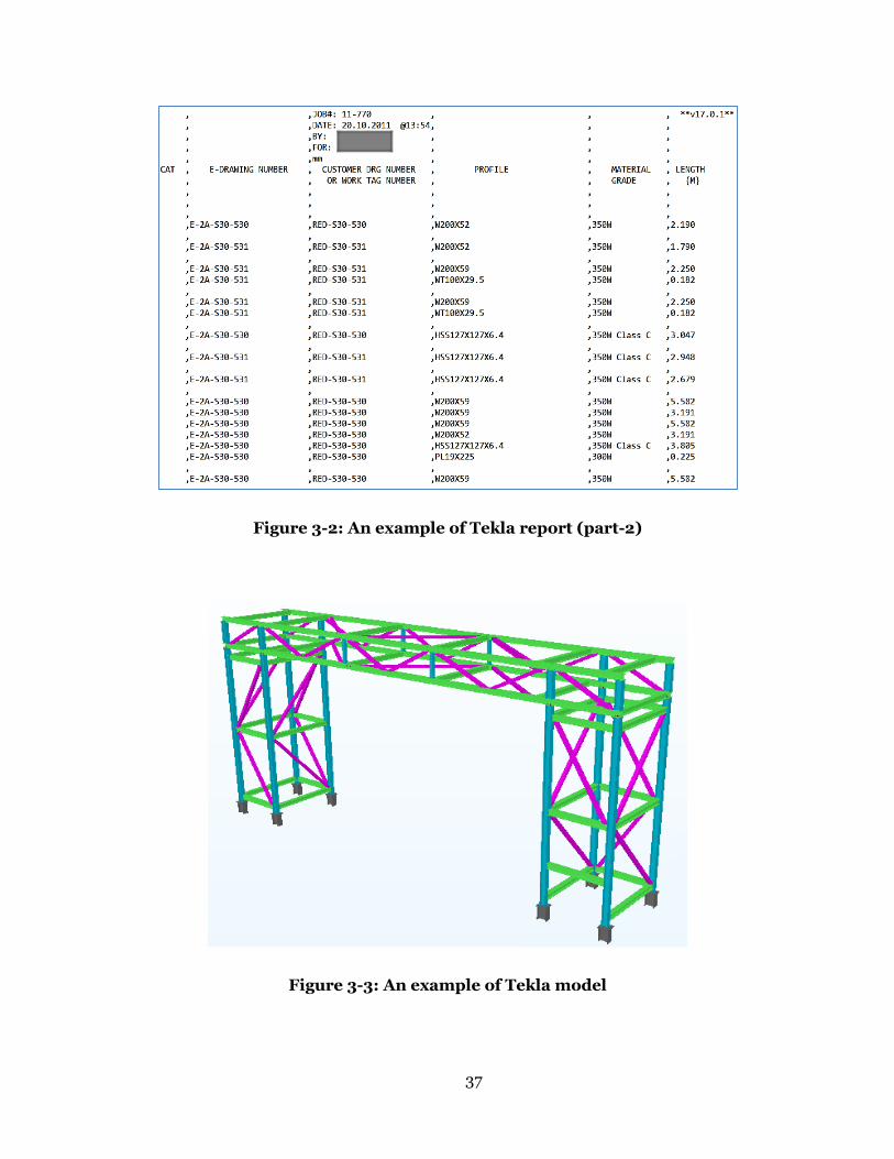
A customized report template (*.rpt) is used in Tekla to create reports
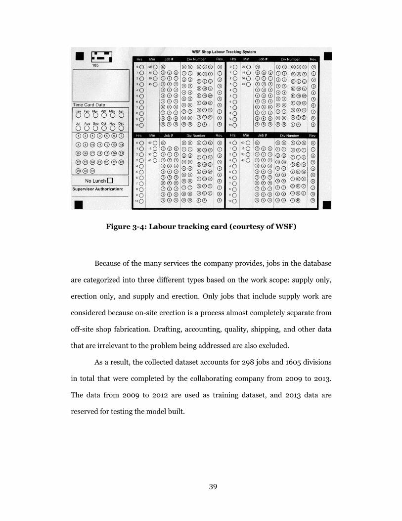
containing necessary information from the BIM models. Figure 3-1 and Figure
3-2 demonstrate an example of a material parts report generated from Tekla, the
original model of which is shown in Figure 3-3. In the report, essential material
attributes, such as part number, description, quantity, length, unit weight, and
drawing number, are listed.
Besides the BIM-based models and reports, the collaborating company’s
information management system (IMS) also includes an internal central database.
There are over 400 tables in the SQL Server database maintaining data for shop
fabrication, as well as drafting, accounting, quality control, shipping, etc. The
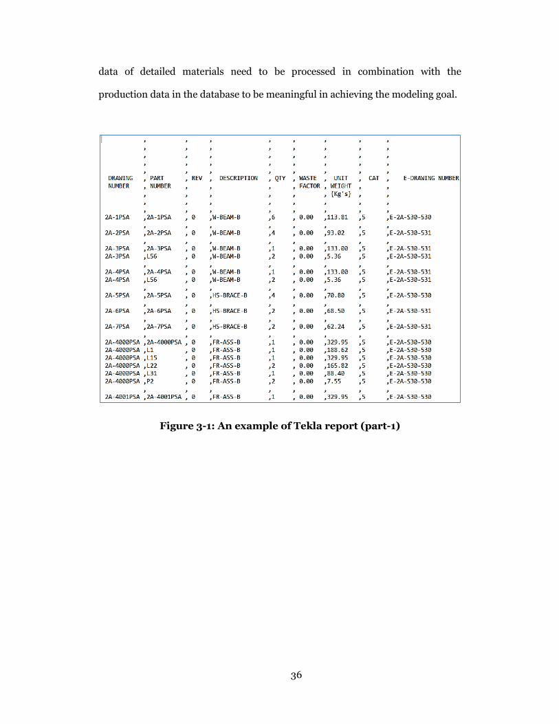
36
data of detailed materials need to be processed in combination with the
production data in the database to be meaningful in achieving the modeling goal.
Figure 3-1: An example of Tekla report (part-1)
37
Figure 3-2: An example of Tekla report (part-2)
Figure 3-3: An example of Tekla model

38
3.2 DATA SELECTION
The targeted IMS contains data dating back over ten years. The
productivity that can be achieved in the shop and the amount of resource
required for fabricating the same amount of structural steel have both changed,
compared with those ten years ago, on account of the technological evolution in
fabrication methods and equipment, the growth of economy, as well as the
development of company strategies. Therefore the input of the learning process
must be recent enough to produce meaningful results that could benefit current
practices. Furthermore, the dataset should be big enough to be representative of
the trade, to contain useful features, and to be able to be split into training and
test datasets.
In addition, the method of time-tracking and recording is always
improved on the shop floor, but errors still exist in historical data for reasons
such as assigning hours to the wrong division number, failure to keep track of
time, and failure to digitalize physical timesheets properly. To reduce noise in
data as much as possible, division records that have zero tonnage, zero budgeted
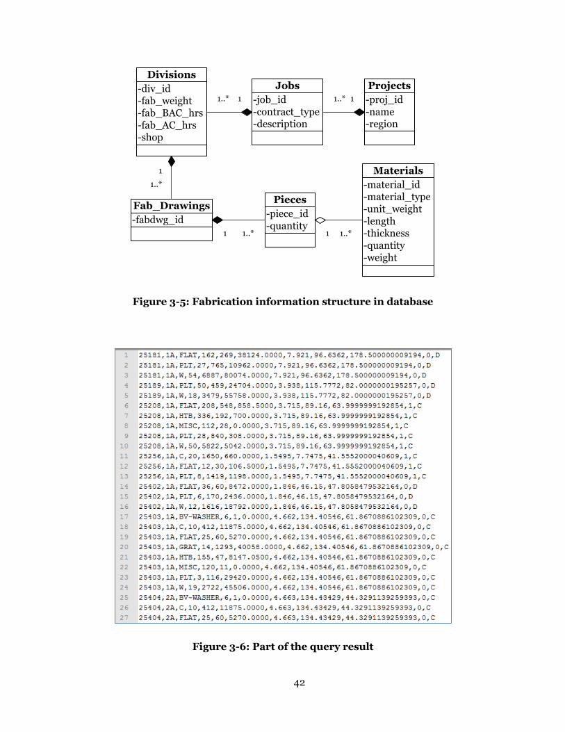
hours or zero actual hours are excluded. The figure below is the paper timecard
currently utilized at the collaborating company.
39
Figure 3-4: Labour tracking card (courtesy of WSF)
Because of the many services the company provides, jobs in the database
are categorized into three different types based on the work scope: supply only,
erection only, and supply and erection. Only jobs that include supply work are
considered because on-site erection is a process almost completely separate from
off-site shop fabrication. Drafting, accounting, quality, shipping, and other data
that are irrelevant to the problem being addressed are also excluded.
As a result, the collected dataset accounts for 298 jobs and 1605 divisions
in total that were completed by the collaborating company from 2009 to 2013.
The data from 2009 to 2012 are used as training dataset, and 2013 data are
reserved for testing the model built.

40
3.3 DATA PREPROCESSING
Having selected the data, preprocessing is necessary to get the data into a
form suitable for machine learning. It is an important step that involves a lot of
iterations, analysis, and exploration.
The selected data are in a relational database and flat files (*.xsr), and are
not ready for application of machine learning algorithms. In the central database,
the production-related data are scattered over several tables. A general
illustration of the object relations is illustrated in Figure 3-5. The table columns
in the figure are only partial. The physical steel materials are not directly
associated with each division, but rather as parts of pieces and fabrication
drawings. Divisions are assigned to different shops to be processed according to
the characteristics of the division and the shops’ capacities. Therefore the shop
name is included as a nominal input of the model. A detailed description of the
relational database structure can be found in Section 3.3.1 - Database Structure.
The database has evolved over the years, leaving misleading parameters
and design problems in it. Without any well-written development logs or
comments available, it took a lot of time to find the proper database tables and
fields to be used for machine learning. A few lessons learnt from working on a
production database are listed below.
Read-only access is not enough. Ask the database administrator
for write permission to allow the use of temporary tables, variables,
and the viewing of stored procedures.
Ensure nothing has changed to avoid affecting the functionality of
the production database.

41
Read all the SQL source code in detail, including data table
structures, constraints, stored procedures, functions, etc.
Comments in the source code may not be reliable. Always test the
functions and keep adequate records.
A same field (or attribute) name used in two tables may mean
different things.
Do not assume the data type of an attribute solely based on its
name. For example, “ID” does not have to be number; it can also
be string.
Starting from a small amount of data makes it easier to verify the
query or calculation results.
Always check any constraints added to a table.
When a foreign key constraint is included in a query, make sure all
fields covered by the foreign key constraint are considered to avoid
duplicate query results.
Data were collected via SQL queries and exported to comma-separated
values (CSV) files. Figure 3-6 is what the raw query result looks like. Records are
at the material level grouped by the division number and different material types.
42
Figure 3-5: Fabrication information structure in database
Figure 3-6: Part of the query result
-job_id-contract_type-description
Jobs-div_id-fab_weight-fab_BAC_hrs-fab_AC_hrs-shop
Divisions
11..*
-fabdwg_id
Fab_Drawings-piece_id-quantity
Pieces
-material_id-material_type-unit_weight-length-thickness-quantity-weight
Materials1
1..*
1 1..* 1 1..*
-proj_id-name-region
Projects11..*

43
However, in order to study the productivity and schedule data at the
division level, the detailed data of all the materials within the same division need
to be collected and then aggregated to the division level. The basic attributes were
collected at the level of each material type. Then the total quantity or length, and
weight was summarized at the division level. A parser program was written in C#
to do the summarization and transposition operations. Material data that belong
to a same division were aggregated as one line item.
In addition, some of the data collected were in imperial units (feet, inch,
and pound); others were in metric units (meter, centimeter, kilogram, and ton).
The data need to have the same scale and unit. Scaling and unit conversion was
also automated by the program.
3.3.1 Database Structure
The concept, project, is used for jobs that are too large to be managed as
one. For example, in oil sands industry there are always multiple construction
projects ongoing at the same time at one mining site. The name of the site can be
used as the name of a project, and all the projects that take place at that site are
considered as jobs under the same project, coded with the same project number.
Once a contract is awarded, a job number is allocated following the naming
convention “XX-YYY”. “XX” is the last two digits of the year when the contract is
awarded. “YYY” is an incremental number ranging from 001 to 999, which is
tracked by a master logbook. Generally small job numbers are assigned for orders
that are less than a certain amount of monetary value or man-hours; large jobs
have large job numbers.
As mentioned in Section 1.2, Figure 1-2, jobs are divided into several
divisions as the basic management unit. The assignment rules include location,

44
scope, structural type, etc. For example, the ladders and handrails within one job
are generally separated from the other steel elements as one division. For a
typical stair tower, each floor may be viewed as a division. Division numbers are
coded in the format of “[0-9][0-9][A-Z]” customarily.
In the underlying database implementation, divisions are further divided
and represented by subdivisions. Generally a division has only one subdivision,
which is its main subdivision. Every division has one and only one main
subdivision. In situations with handrails and ladders, a separate subdivision is
created using the same division number. Subdivision tables contain all the
schedule-related data, including all the milestones, planned dates, actual dates,
detailer ID, fabrication requirements, etc. The division tables contain the general
description, modification timestamps, information about cost categories, man-
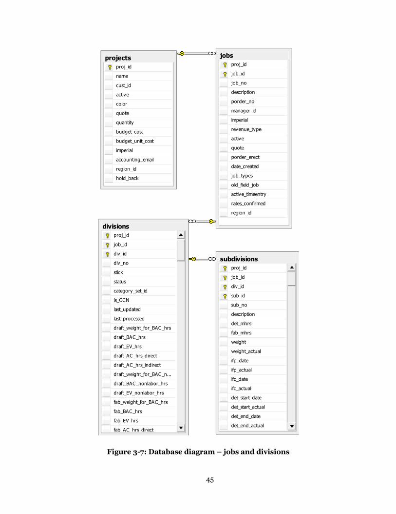
hour tracking data, etc. The relational diagram of the four tables (projects, jobs,
divisions, and subdivisions) is in Figure 3-7.
45
Figure 3-7: Database diagram – jobs and divisions
divisions
proj_id
job_id
div_id
div_no
stick
status
category_set_id
is_CCN
last_updated
last_processed
draft_weight_for_BAC_hrs
draft_BAC_hrs
draft_EV_hrs
draft_AC_hrs_direct
draft_AC_hrs_indirect
draft_weight_for_BAC_n...
draft_BAC_nonlabor_hrs
draft_EV_nonlabor_hrs
fab_weight_for_BAC_hrs
fab_BAC_hrs
fab_EV_hrs
fab_AC_hrs_direct
subdivisions
proj_id
job_id
div_id
sub_id
sub_no
description
det_mhrs
fab_mhrs
weight
weight_actual
ifp_date
ifp_actual
ifc_date
ifc_actual
det_start_date
det_start_actual
det_end_date
det_end_actual
projects
proj_id
name
cust_id
active
color
quote
quantity
budget_cost
budget_unit_cost
imperial
accounting_email
region_id
hold_back
jobs
proj_id
job_id
job_no
description
porder_no
manager_id
imperial
revenue_type
active
quote
porder_erect
date_created
job_types
old_field_job
active_timeentry
rates_confirmed
region_id
46
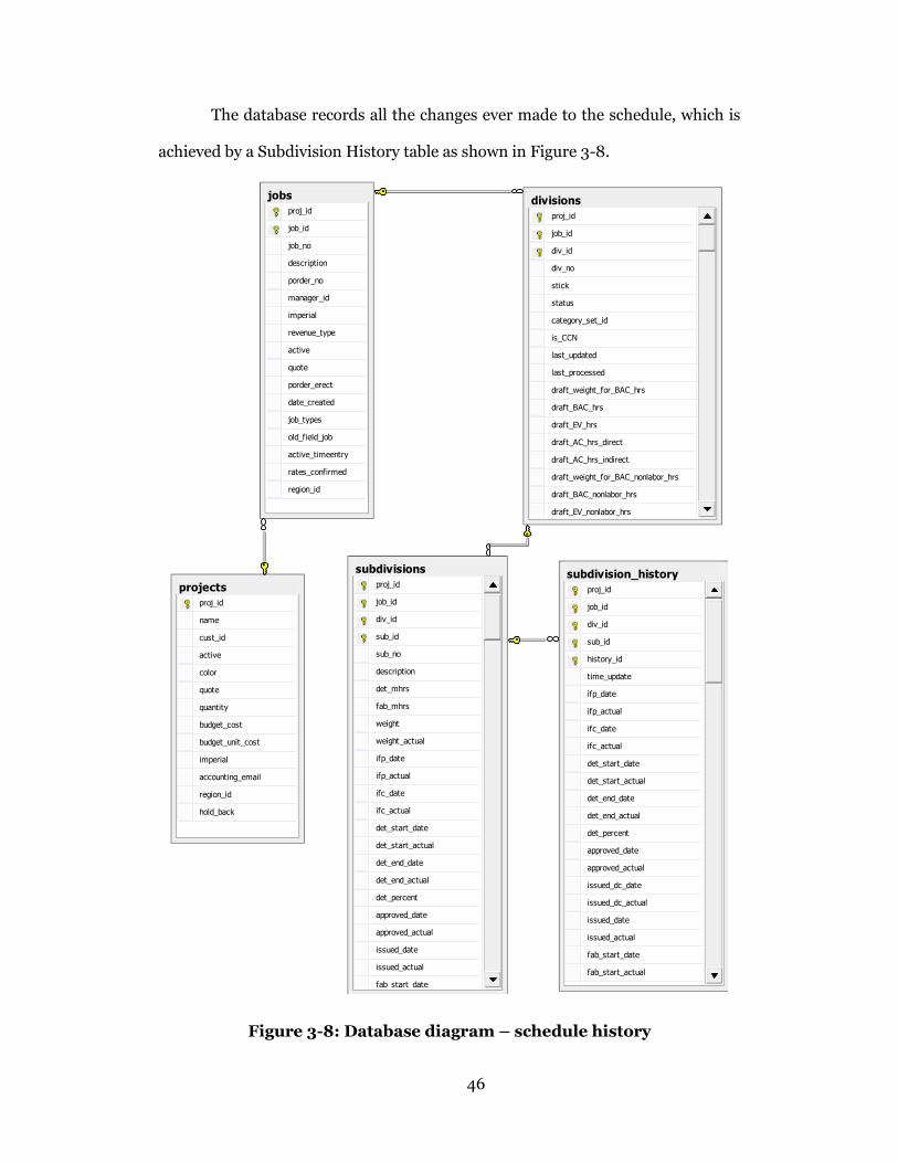
The database records all the changes ever made to the schedule, which is
achieved by a Subdivision History table as shown in Figure 3-8.
Figure 3-8: Database diagram – schedule history
divisions
proj_id
job_id
div_id
div_no
stick
status
category_set_id
is_CCN
last_updated
last_processed
draft_weight_for_BAC_hrs
draft_BAC_hrs
draft_EV_hrs
draft_AC_hrs_direct
draft_AC_hrs_indirect
draft_weight_for_BAC_nonlabor_hrs
draft_BAC_nonlabor_hrs
draft_EV_nonlabor_hrs
subdivisions
proj_id
job_id
div_id
sub_id
sub_no
description
det_mhrs
fab_mhrs
weight
weight_actual
ifp_date
ifp_actual
ifc_date
ifc_actual
det_start_date
det_start_actual
det_end_date
det_end_actual
det_percent
approved_date
approved_actual
issued_date
issued_actual
fab_start_date
projects
proj_id
name
cust_id
active
color
quote
quantity
budget_cost
budget_unit_cost
imperial
accounting_email
region_id
hold_back
jobs
proj_id
job_id
job_no
description
porder_no
manager_id
imperial
revenue_type
active
quote
porder_erect
date_created
job_types
old_field_job
active_timeentry
rates_confirmed
region_id
subdivision_history
proj_id
job_id
div_id
sub_id
history_id
time_update
ifp_date
ifp_actual
ifc_date
ifc_actual
det_start_date
det_start_actual
det_end_date
det_end_actual
det_percent
approved_date
approved_actual
issued_dc_date
issued_dc_actual
issued_date
issued_actual
fab_start_date
fab_start_actual
fab_end_date
47
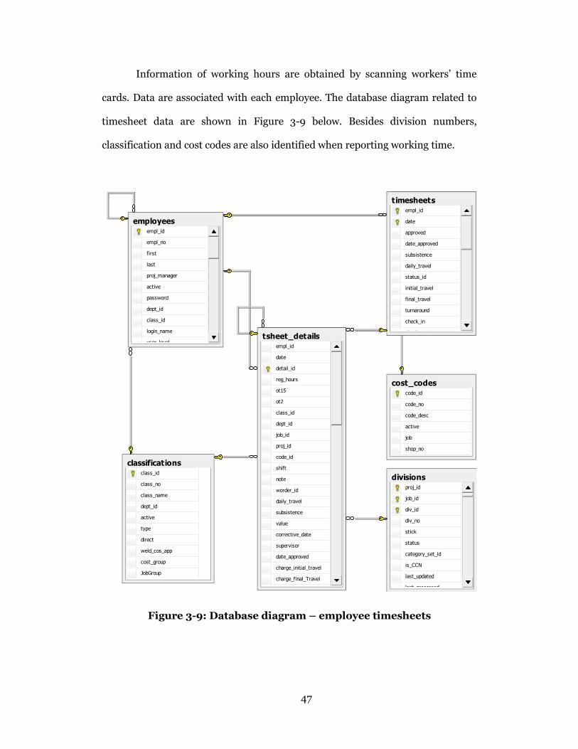
Information of working hours are obtained by scanning workers’ time
cards. Data are associated with each employee. The database diagram related to
timesheet data are shown in Figure 3-9 below. Besides division numbers,
classification and cost codes are also identified when reporting working time.
Figure 3-9: Database diagram – employee timesheets
classificationsclass_id
class_no
class_name
dept_id
active
type
direct
weld_cos_app
cost_group
JobGroup
employeesempl_id
empl_no
first
last
proj_manager
active
password
dept_id
class_id
login_name
user_level
cost_codescode_id
code_no
code_desc
active
job
shop_no
tsheet_detailsempl_id
date
detail_id
reg_hours
ot15
ot2
class_id
dept_id
job_id
proj_id
code_id
shift
note
worder_id
daily_travel
subsistence
value
corrective_date
supervisor
date_approved
charge_initial_travel
charge_final_Travel
charge_turnaround
timesheetsempl_id
date
approved
date_approved
subsistence
daily_travel
status_id
initial_travel
final_travel
turnaround
check_in
check_out
divisionsproj_id
job_id
div_id
div_no
stick
status
category_set_id
is_CCN
last_updated
last_processed

48
Classification is the type of workforce, such as welders, fitters, labourers,
and foremen. Cost coding is another mechanism to track project performance.
Generally cost items include detailing, document control, engineering, fabrication
labour, freight, galvanizing, grating, material, paint labour, profit, quality control,
etc. Not only the fabrication crew in the shop, all the office employees are all
recorded in the Employees table. Stored procedures and calculated columns are
used to sum up the detailed timesheet information to the division level.
Figure 3-10 shows the connections between divisions, fabrication
drawings, and pieces. All the drawings need to be approved before moving to the
next phase. When the drafting department completes the initial engineering
design, drawings are submitted to the customer for approval. This Issued for
Approval (IFA) date is one of the several important milestones in the fabrication
production cycle. The customer’s reply may be one of the three options: proceed,
revise and proceed, or revise and resubmit. The return date is called Return from
Approval (RFA), another milestone. After that, drawings are issued to Document
Control department for tracking, formatting, and printing to be distributed to
shop for fabrication. A division has one or more than one fabrication drawings. A
drawing has one or more than one steel pieces.
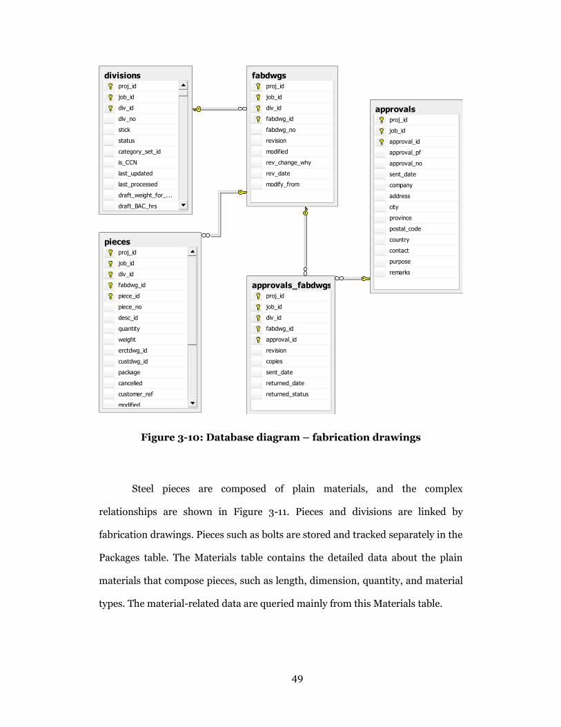
49
Figure 3-10: Database diagram – fabrication drawings
Steel pieces are composed of plain materials, and the complex
relationships are shown in Figure 3-11. Pieces and divisions are linked by
fabrication drawings. Pieces such as bolts are stored and tracked separately in the
Packages table. The Materials table contains the detailed data about the plain
materials that compose pieces, such as length, dimension, quantity, and material
types. The material-related data are queried mainly from this Materials table.
approvalsproj_id
job_id
approval_id
approval_pf
approval_no
sent_date
company
address
city
province
postal_code
country
contact
purpose
remarks
approvals_fabdwgsproj_id
job_id
div_id
fabdwg_id
approval_id
revision
copies
sent_date
returned_date
returned_status
piecesproj_id
job_id
div_id
fabdwg_id
piece_id
piece_no
desc_id
quantity
weight
erctdwg_id
custdwg_id
package
cancelled
customer_ref
modified
fabdwgsproj_id
job_id
div_id
fabdwg_id
fabdwg_no
revision
modified
rev_change_why
rev_date
modify_from
divisionsproj_id
job_id
div_id
div_no
stick
status
category_set_id
is_CCN
last_updated
last_processed
draft_weight_for_...
draft_BAC_hrs
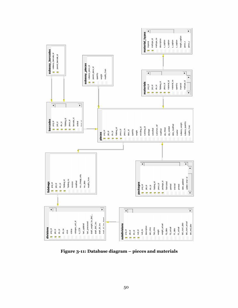
50
Figure 3-11: Database diagram – pieces and materials
divisions
proj_id
job_id
div_id
div_no
stick
status
category_set_id
is_CCN
last_updated
last_processed
draft_weight_for_BAC...
draft_BAC_hrs
draft_EV_hrs
draft_AC_hrs_direct
subdivisions
proj_id
job_id
div_id
sub_id
sub_no
description
det_mhrs
fab_mhrs
weight
weight_actual
ifp_date
ifp_actual
ifc_date
ifc_actual
det_start_date
det_start_actual
det_end_date
pieces
proj_id
job_id
div_id
fabdwg_id
piece_id
piece_no
desc_id
quantity
weight
erctdwg_id
custdwg_id
package
cancelled
customer_ref
modified
qty_fitted
qty_welded
date_modified
counter
subassy_weight
subassy_quantity
modify_from
fabdwgs
proj_id
job_id
div_id
fabdwg_id
fabdwg_no
revision
modified
rev_change_why
rev_date
modify_from
subassy_pieces
subassy_piece_id
parent_piece_id
quantity
weight
modify_from
subassy_barcodes
subassy_barcode_id
parent_barcode_id
barcodes
proj_id
job_id
div_id
fabdwg_id
piece_id
barcode_id
ordinal
final_id
packages
proj_id
job_id
div_id
fabdwg_id
piece_id
package_id
fabricated
painted
erected
printed
date_updated
update_empl_id
materials
proj_id
job_id
div_id
fabdwg_id
piece_id
material_id
material_no
quantity
imperial
mattype_id
material_types
imperial
mattype_id
mattype_no
description
s_caption
x_caption
y_caption
z_caption
length_caption
parse_x
parse_y

51
3.4 DATA TRANSFORMATION
Weight and length are two dependent parameters of steel materials, and it
would be more meaningful to the problem if they are aggregated into a single
feature. The unit weight per unit length, for example “kg/m,” and quantity are the
two most basic attributes of steel materials. For major materials such as beams,
columns, and channels, the fabrication man-hours required are positively
correlated with the material length and weight, but for the various kinds of bolts
and nuts used in the shop, quantity is a much more meaningful factor to be
considered. The length of a bolt plays no role in determining the handling time of
the piece it is attached to. Whether the bolt is long or short, it is the quantity that
truly matters. The feature aggregation is done during the parsing process.
Table 3-1 lists the 45 material types examined in this study, according to
the collaborating company’s information library. The letters before the dash sign
“-” are the abbreviations and the part after it are the complete description of the
material type. For example, “W”-shaped steel actually refers to wide flange beams,
and its key attribute is the length instead of quantity. Materials such as
miscellaneous assemblies are excluded since their amounts and fabrication
requirements are too small to make a difference.
Table 3-1: Material types and key attributes
Material Type Key Attribute
W – Wide Flange Beams Length
L – Equal Legs Length
L – Unequal Legs Length
C – Channels Length
HS – Square Hollow Steel Sections Length
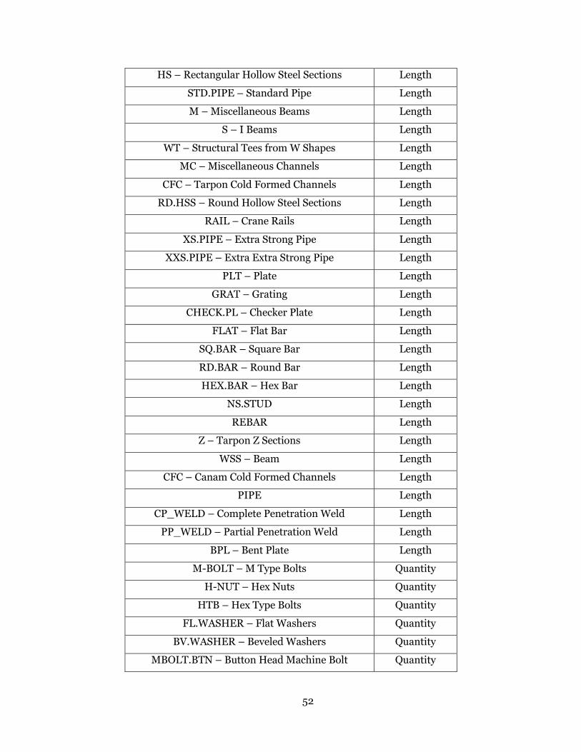
52
HS – Rectangular Hollow Steel Sections Length
STD.PIPE – Standard Pipe Length
M – Miscellaneous Beams Length
S – I Beams Length
WT – Structural Tees from W Shapes Length
MC – Miscellaneous Channels Length
CFC – Tarpon Cold Formed Channels Length
RD.HSS – Round Hollow Steel Sections Length
RAIL – Crane Rails Length
XS.PIPE – Extra Strong Pipe Length
XXS.PIPE – Extra Extra Strong Pipe Length
PLT – Plate Length
GRAT – Grating Length
CHECK.PL – Checker Plate Length
FLAT – Flat Bar Length
SQ.BAR – Square Bar Length
RD.BAR – Round Bar Length
HEX.BAR – Hex Bar Length
NS.STUD Length
REBAR Length
Z – Tarpon Z Sections Length
WSS – Beam Length
CFC – Canam Cold Formed Channels Length
PIPE Length
CP_WELD – Complete Penetration Weld Length
PP_WELD – Partial Penetration Weld Length
BPL – Bent Plate Length
M-BOLT – M Type Bolts Quantity
H-NUT – Hex Nuts Quantity
HTB – Hex Type Bolts Quantity
FL.WASHER – Flat Washers Quantity
BV.WASHER – Beveled Washers Quantity
MBOLT.BTN – Button Head Machine Bolt Quantity

53
MBOLT.HEX – Hex Head Machine Bolt Quantity
HILTI.HAS – Threaded Anchor Rods Quantity
HILTI-HVU – Adhesive Capsules Quantity
HILTI-HIT – Adhesive Anchor Cartridges Quantity
HILTI-KB3 – Expansion Anchor Bolts Quantity
HILTI.HSL3 – Heavy Duty Expansion Anchor Bolts Quantity
DTI.WASHER – Compressible Washers with DTI Quantity
The outcome of the program is a CSV file ready for WEKA with each line
representing one division. The format of the output file is demonstrated in Figure
3-12.
Figure 3-12: Formatted SQL data

54
To illustrate the transformed data structure better, Table 3-2 lists the
characteristics of one of the divisions to be fed into WEKA. All zero-valued
attributes were not included in the table.
Table 3-2: Sample data of a division
Characteristics Division-i Note
Division ID 18117 Input
Division Weight (kg) 28373 Input
Shop (“A”, “B”, “C”, or “D”) “A” Input
W Length (m) 13.89 Input
L Length (m) 9.27 Input
Plate Length (m) 78.06 Input
Flat Bar Length (m) 8.07 Input
Hex Type Bolts Quantity 381 Input
Fabrication Actual MHrs 875.57 Targeted Output
Fabrication Budget MHrs 692.30 Expert Judgment
In conclusion, the whole process of preparing the dataset for machine
learning is summarized in Figure 3-13. A training dataset and a test dataset, each
as a CSV file, are prepared for machine learning modeling, the detailed process of
which is illustrated in the next chapter.
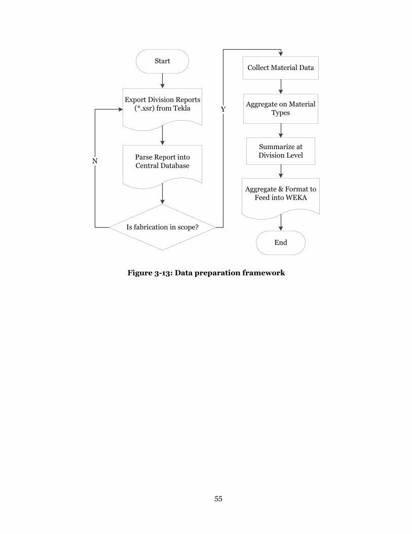
55
Figure 3-13: Data preparation framework
StartCollect Material Data
Is fabrication in scope?
Aggregate on Material Types
Summarize at Division Level
End
Parse Report into Central Database
Export Division Reports (*.xsr) from Tekla
Aggregate & Format to Feed into WEKA
N
Y

56
Chapter 4. MODEL SELECTION & EVALUATION
4.1 CANDIDATE MODELS
Various types of models were investigated during the stage of model
building and training. To obtain statistically meaningful results, 10 runs of 10-
fold stratified cross-validation were performed on the training dataset, which is
the production data collected from 2009 to 2012, using different schemes. 10
iterations of 10-fold cross-validation means 100 calls of each scheme with the
same dataset (Bouckaert et al. 2014). Related knowledge about cross validation
can be found in Section 2.4.5 - Evaluation of Machine Learning Algorithms.
It is generally believed that the more materials a job requires, the more
man-hours it will cost. Accordingly, linear regression could be a suitable
technique to use for quantitative man-hour prediction. The Linear Regression
implementation in WEKA uses the Akaike information criterion (AIC) (Burnham
and Anderson 2002) for model selection. AIC is a means for measuring the
relative quality of a statistical model given a set of data. It rewards goodness of fit
of the model, but penalizes increasing the number of parameters so as to lead to
over-fitting. A statistical selection procedure is also incorporated in WEKA to
determine the best combination of independent input variables. Details about the
selected factors and the regression parameters are provided in Equation (1) in
Section 4.3 - Evaluation on Test Dataset.
Although ANN models are generally popular in the construction industry,
they are more suitable for non-linear problems. One of the most widely used ANN,
Radial Basis Function (RBF) neural network, was tested in this study for
comparison. The workflow of RBF can be found in Section 2.4.4 - RBF Neural
57
Network. One of the parameters, the number of clusters, was empirically set as
the number of shops, which is 4 for the collaborating company.
Moreover, a Support Vector Machine with Sequential Minimal
Optimization (SMO) algorithm (Platt 1998; Shevade et al. 2000) was also
investigated. In Support Vector Regression (SVR), an objective function on the
training set is defined with a constraint threshold, and the optimization target of
regression is to find the best fit objective function while excluding the least
outlying training data (Smola and Schölkopf 2004). The basic idea of SVR can be
found in Section 2.4.3 - SVM Regression.
Some other models were also tested, such as:
Least median squared linear regression
M5P tree
Multilayer perceptron
The modeling results were not good or typical enough to be elaborated in
detail.
4.2 CROSS VALIDATION
The dataset from 2009 to 2012, which accounts for 248 jobs and 1343
divisions out of the total 298 jobs and 1605 divisions, was used to train the model.
Data in 2013 were collected as an independent dataset and reserved for further
testing. Various schemes were evaluated by performing 10-fold cross-validation
on the 2009 – 2012 dataset.
The visualization of classifier errors of the results is shown in Figure 4-3,
Figure 4-4, and Figure 4-5. The horizontal axis represents actual fabrication man-
hours; the vertical axis represents the man-hour prediction calculated through
the trained models. The closer the data points are aligned on the 45 degree line,
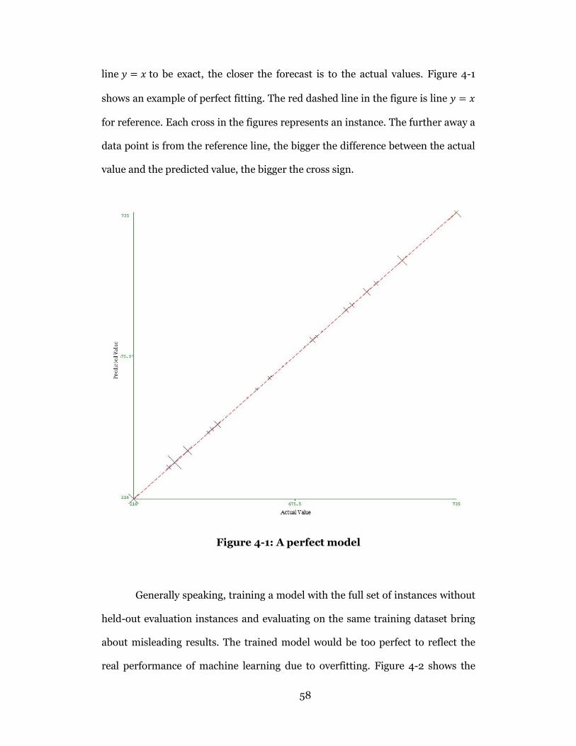
58
line 𝑦 = 𝑥 to be exact, the closer the forecast is to the actual values. Figure 4-1
shows an example of perfect fitting. The red dashed line in the figure is line 𝑦 = 𝑥
for reference. Each cross in the figures represents an instance. The further away a
data point is from the reference line, the bigger the difference between the actual
value and the predicted value, the bigger the cross sign.
Figure 4-1: A perfect model
Generally speaking, training a model with the full set of instances without
held-out evaluation instances and evaluating on the same training dataset bring
about misleading results. The trained model would be too perfect to reflect the
real performance of machine learning due to overfitting. Figure 4-2 shows the

59
testing result of RBF neural network using the training dataset itself. Even in this
best possible test scenario, the points in Figure 4-2 are far from being a good fit
as shown in Figure 4-1. It is clear that the trained model is not suitable for the
defined problem.
Figure 4-2: Evaluation of RBF network using training set
Figure 4-3 is the result of cross validation using the same dataset and
model training. As expected, the results are unsatisfactory based on the current
problem definition and dataset available. A summary of the evaluation statistics
can be found in Table 4-1.
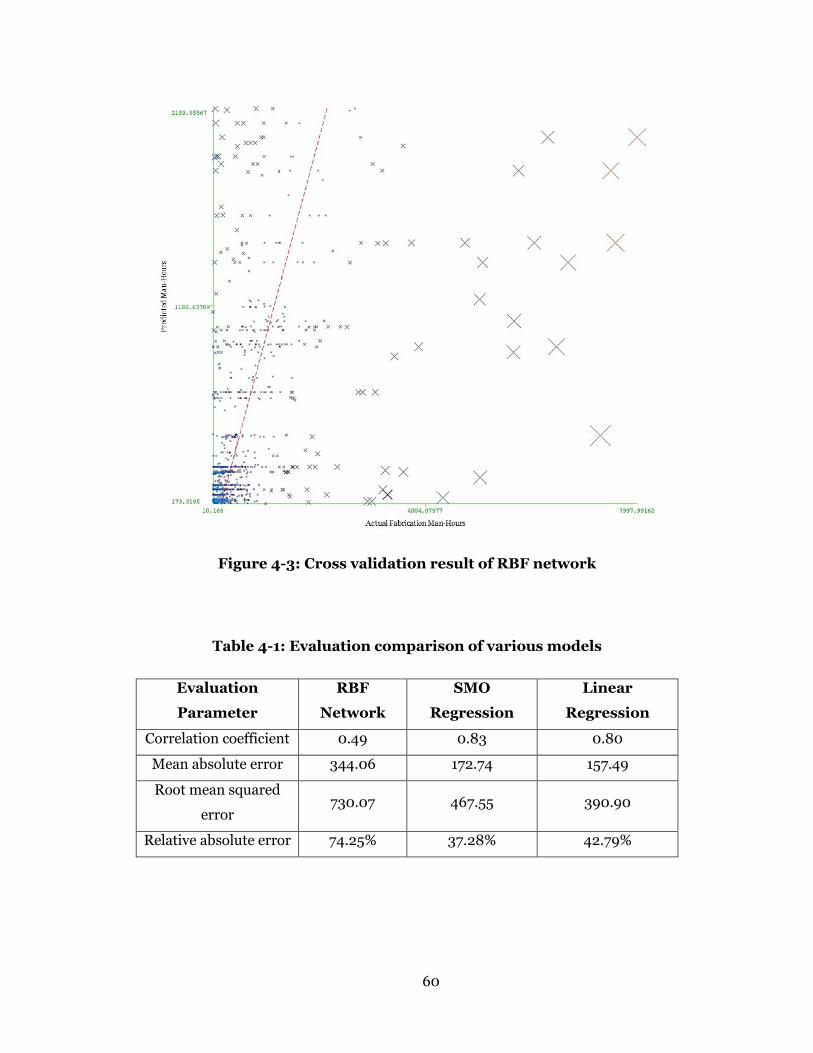
60
Figure 4-3: Cross validation result of RBF network
Table 4-1: Evaluation comparison of various models
Evaluation
Parameter
RBF
Network
SMO
Regression
Linear
Regression
Correlation coefficient 0.49 0.83 0.80
Mean absolute error 344.06 172.74 157.49
Root mean squared
error 730.07 467.55 390.90
Relative absolute error 74.25% 37.28% 42.79%
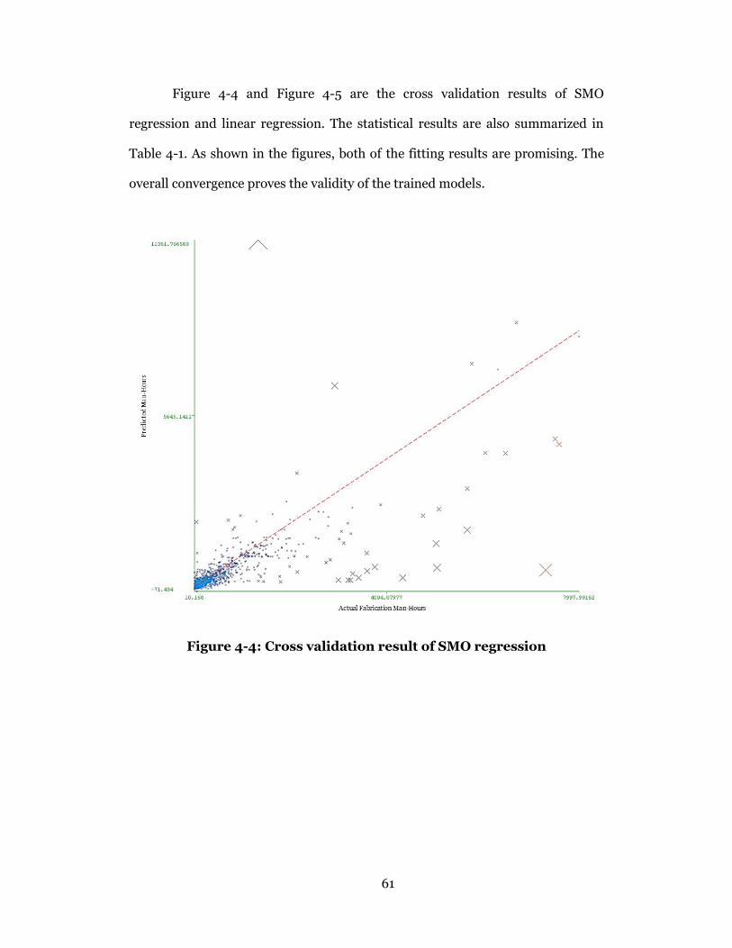
61
Figure 4-4 and Figure 4-5 are the cross validation results of SMO
regression and linear regression. The statistical results are also summarized in
Table 4-1. As shown in the figures, both of the fitting results are promising. The
overall convergence proves the validity of the trained models.
Figure 4-4: Cross validation result of SMO regression
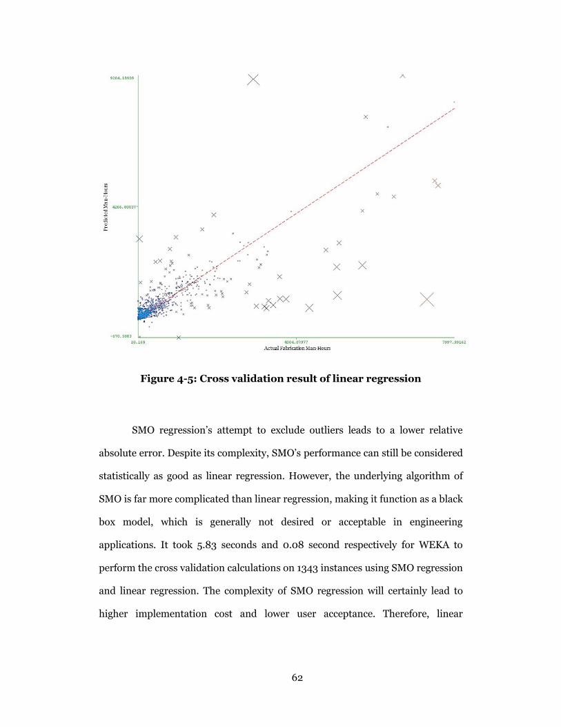
62
Figure 4-5: Cross validation result of linear regression
SMO regression’s attempt to exclude outliers leads to a lower relative
absolute error. Despite its complexity, SMO’s performance can still be considered
statistically as good as linear regression. However, the underlying algorithm of
SMO is far more complicated than linear regression, making it function as a black
box model, which is generally not desired or acceptable in engineering
applications. It took 5.83 seconds and 0.08 second respectively for WEKA to
perform the cross validation calculations on 1343 instances using SMO regression
and linear regression. The complexity of SMO regression will certainly lead to
higher implementation cost and lower user acceptance. Therefore, linear

63
regression is selected as the solution to the quantity take-off problem in the
context of structural steel fabrication.
4.3 EVALUATION ON TEST DATASET
The best-fit model trained by linear regression is shown in Equation (4-1)
below. The number of fabrication man-hours a division requires can be calculated
based on some key properties that are obtained from BIM models. The complete
list of attributes can be found in Table 3-1.
054.154215.340.4813.0
.5694.1.776.10.7614.1
.6684.0.29.0.1164.2
1334.01645.0.5089.11
.4317.50.4378.2.8187.0
7095.02687.07115.61708.0
9271.02036.0015.0
FabAHEXMBOLT
WELDPPWELDCPSTUDNS
WASHERBVWASHERFLPLCHECK
HTBPLTPIPEXXS
PIPEXSPIPESTDHSSRD
HSLMCC
WTWdivWtdivAct
(4-1)
Basic information about the input and output variables are shown in
Table 4-2 below. The average values and ranges were based on the whole dataset,
i.e. fabrication data from 2009 to 2013.
Table 4-2: Information about variables in Equation (4-1)
Variable Description Unit Average Range
divAct Division actual MHrs Man-Hour 454.16 [10.17,
7997.99]
divWt Division weight Kilogram 17877.76 [1001,
238169]
W Length of wide flange beams Meter 135.35 [0, 2050.66]
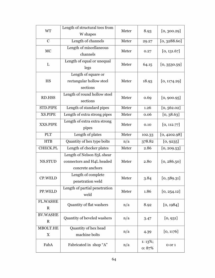
64
WT Length of structural tees from
W shapes Meter 8.93 [0, 300.29]
C Length of channels Meter 29.27 [0, 3288.60]
MC Length of miscellaneous
channels Meter 0.27 [0, 131.67]
L Length of equal or unequal
legs Meter 64.15 [0, 3530.59]
HS
Length of square or
rectangular hollow steel
sections
Meter 18.93 [0, 1174.29]
RD.HSS Length of round hollow steel
sections Meter 0.69 [0, 900.95]
STD.PIPE Length of standard pipes Meter 1.26 [0, 562.02]
XS.PIPE Length of extra strong pipes Meter 0.06 [0, 38.63]
XXS.PIPE Length of extra extra strong
pipes Meter 0.10 [0, 112.77]
PLT Length of plates Meter 102.33 [0, 4202.98]
HTB Quantity of hex type bolts n/a 378.82 [0, 9235]
CHECK.PL Length of checker plates Meter 2.86 [0, 209.53]
NS.STUD
Length of Nelson S3L shear
connectors and H4L headed
concrete anchors
Meter 2.80 [0, 286.50]
CP.WELD Length of complete
penetration weld Meter 3.84 [0, 589.31]
PP.WELD Length of partial penetration
weld Meter 1.86 [0, 254.12]
FL.WASHE
R Quantity of flat washers n/a 8.92 [0, 1984]
BV.WASHE
R Quantity of beveled washers n/a 3.47 [0, 931]
MBOLT.HE
X
Quantity of hex head
machine bolts n/a 4.39 [0, 1176]
FabA Fabricated in shop “A” n/a 1: 13%;
0: 87% 0 or 1
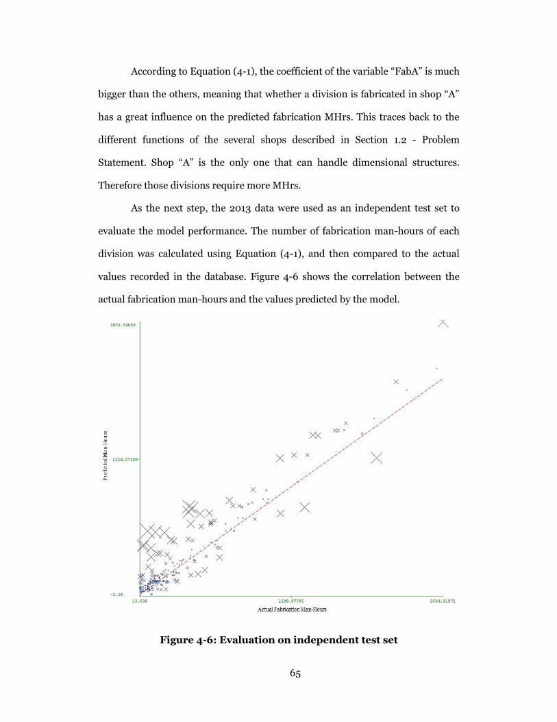
65
According to Equation (4-1), the coefficient of the variable “FabA” is much
bigger than the others, meaning that whether a division is fabricated in shop “A”
has a great influence on the predicted fabrication MHrs. This traces back to the
different functions of the several shops described in Section 1.2 - Problem
Statement. Shop “A” is the only one that can handle dimensional structures.
Therefore those divisions require more MHrs.
As the next step, the 2013 data were used as an independent test set to
evaluate the model performance. The number of fabrication man-hours of each
division was calculated using Equation (4-1), and then compared to the actual
values recorded in the database. Figure 4-6 shows the correlation between the
actual fabrication man-hours and the values predicted by the model.
Figure 4-6: Evaluation on independent test set

66
The method of tracking and recording actual hours on the shop floor has
been gradually enhanced. New working procedures of timesheet recording and
division planning have been formalized and emphasized. Shop workers are more
used to and better at recording their working time accurately over the past few
years. The historical data can have errors due to inaccurate records, for instance,
working hours assigned to the wrong division number. Compared to the
visualization in Figure 4-5, which is the cross validation results on historical data ,
points of 2013 data in Figure 4-6 suggests better convergence. The reason for this
can be partially due to the improved tracking and recording of actual hours.
Limitations in the data are also revealed in the figure. For some divisions,
the model tends to predict the work to be more than the actual man-hours
recorded. One reason may be that when a worker is working on multiple divisions
in a day, it is very likely that he fails to precisely track the number of hours he has
spent in each division. Nevertheless, the figure clearly demonstrates that the
trained model can be considered satisfactory in terms of accuracy for rendering
decision support for estimators to predict the fabrication man-hours.
To further evaluate the performance of the prediction model, the relative
difference results were plotted in Figure 4-7.
𝑅𝑒𝑙𝑎𝑡𝑖𝑣𝑒 𝐷𝑖𝑓𝑓𝑒𝑟𝑒𝑛𝑐𝑒 =|𝑝𝑖−𝑎𝑖|
𝑎𝑖 (4-2)
where 𝑝𝑖 is the value predicted by the model and 𝑎𝑖 is the actual value.
For example, as shown in the figure, 68 of the 262 divisions in the test
dataset, or 26% of the test dataset, have relative differences less than 10%. 44
divisions, or 17% of the test dataset, have relative differences that are between 10%
and 20%. The “small” series in Figure 4-7 represents divisions whose actual
MHrs, or workload, are less than 48 MHrs. It is clear that more than half of the
large prediction errors (relative difference > 100%) are small divisions.

67
Figure 4-7: Prediction results of test dataset
Sensitivity analysis was conducted in order to test the sensitivity of the
model output to changes in the input variables. Each of the input variables were
modified while the values of the other variables were kept constant to determine
their respective impact on the prediction result. Thus the variations in the
prediction results would be under the exclusive influence of the one factor under
study (El-Abbasy et al. 2014). The values of the variable under study were varied
from 𝑚𝑖𝑛 + 𝑝 to 𝑚𝑎𝑥 = 𝑚𝑖𝑛 + 10𝑝 , where 𝑝 was calculated by Equation (4-3)
below.
𝑝 =𝑀𝑎𝑥−𝑀𝑖𝑛
10 (4-3)
𝑀𝑎𝑥 and 𝑀𝑖𝑛 are the maximum and minimum values in each factor’s
corresponding data space.
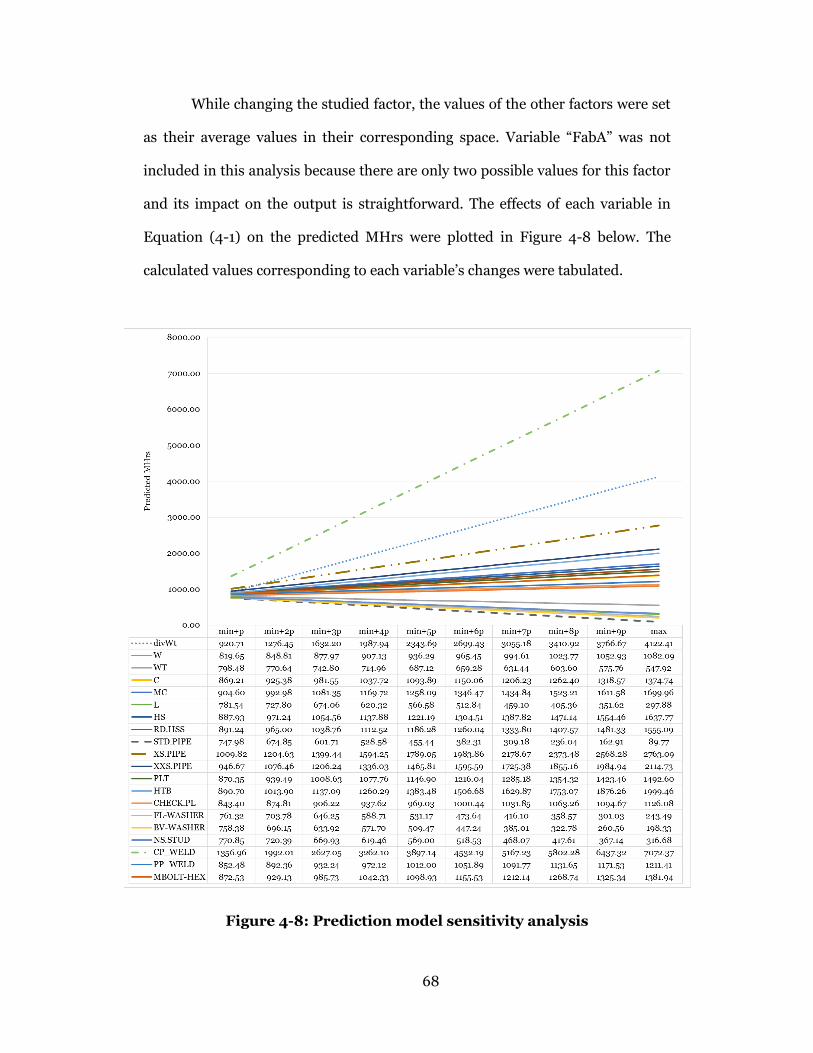
68
While changing the studied factor, the values of the other factors were set
as their average values in their corresponding space. Variable “FabA” was not
included in this analysis because there are only two possible values for this factor
and its impact on the output is straightforward. The effects of each variable in
Equation (4-1) on the predicted MHrs were plotted in Figure 4-8 below. The
calculated values corresponding to each variable’s changes were tabulated.
Figure 4-8: Prediction model sensitivity analysis
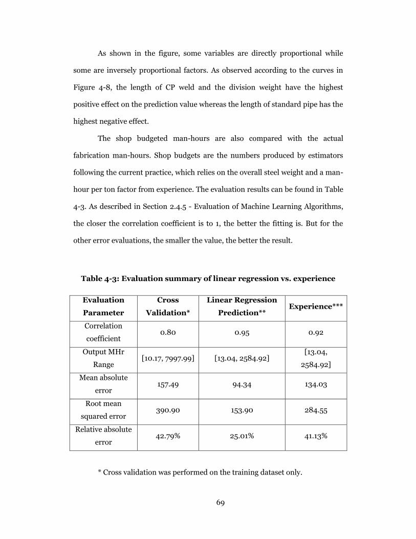
69
As shown in the figure, some variables are directly proportional while
some are inversely proportional factors. As observed according to the curves in
Figure 4-8, the length of CP weld and the division weight have the highest
positive effect on the prediction value whereas the length of standard pipe has the
highest negative effect.
The shop budgeted man-hours are also compared with the actual
fabrication man-hours. Shop budgets are the numbers produced by estimators
following the current practice, which relies on the overall steel weight and a man-
hour per ton factor from experience. The evaluation results can be found in Table
4-3. As described in Section 2.4.5 - Evaluation of Machine Learning Algorithms,
the closer the correlation coefficient is to 1, the better the fitting is. But for the
other error evaluations, the smaller the value, the better the result.
Table 4-3: Evaluation summary of linear regression vs. experience
Evaluation
Parameter
Cross
Validation*
Linear Regression
Prediction** Experience***
Correlation
coefficient 0.80 0.95 0.92
Output MHr
Range [10.17, 7997.99] [13.04, 2584.92]
[13.04,
2584.92]
Mean absolute
error 157.49 94.34 134.03
Root mean
squared error 390.90 153.90 284.55
Relative absolute
error 42.79% 25.01% 41.13%
* Cross validation was performed on the training dataset only.

70
** The prediction was for the test dataset using the model trained by
training dataset.
*** Experience represents the expert estimation on the test dataset.
The forecasted results are closer to the actual values than the judgment
made by the professional judgment and experience. The increased accuracy in
quantity takeoff will help optimize the company’s resource allocation and reduce
the risk of cost and schedule overrun. More importantly, the model can be useful
as decision support or guidance for someone with little or no experience,
especially when no detailed estimating handbook or manual, except a procedure
guideline, is available. The estimating process can be accelerated and managers
better assured.

71
Chapter 5. SHOP LOADING TOOLS
5.1 BACKGROUND
Resources in structural steel fabrication shops include specialized
stationary and portable machines, equipment, and workers. Constrained by the
available resources, the fabricator’s strategies, and/or contractual requirements,
the workload in a steel fabrication shop needs to be carefully scheduled. There are
always multiple jobs taking place in a fabrication shop at the same time, with
different schedules. The ideal situation is to maintain a stable or mildly
fluctuating level in the total working man-hours in each particular shop.
In the collaborating company, when the Shop Operations Manager works
with a Project Manager to come up with a schedule for a job, they need to enter
the fabrication plans of each division into the company’s IMS and use the
software to spread the workload over time in order to see the overall fluctuation
in workload of all the divisions. It takes time to enter the data into the system,
make adjustments, and re-run the loading report.
In this research, an Excel Macro-Enabled Workbook file (*.xlsm) was
developed to read the estimated man-hours and fabrication schedules of divisions
and generate a summary loading chart for the managers to review. Schedule
changes can be easily made in the spreadsheet and it is convenient to propagate
the report. In addition, a second tool was developed producing a chart comparing
the loading changes resulting from scheduling modification. Detailed Macro code
can be found in Appendix A and Appendix B.

72
5.2 SHOP LOADING TOOL
Excel VBA (Visual Basic for Applications) is the name of the programming
language of Excel, and the loading functions are implemented in VBA.
Figure 5-1 shows the user interface of the shop loading tool. Functional
codes are associated with the two buttons “start” and “clear”. To use the loading
tool, enter division data right below the column headings, with no blank lines in
between. The number of records will be calculated and shown in the
corresponding field. User needs to ensure the number is correct. Then by clicking
the “start” button, the numbers are read and calculated, populating a loading
chart. When finished, the entire workbook can be cleared using the “clear” button.
Figure 5-1: Shop loading tool user interface
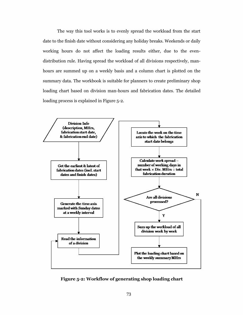
73
The way this tool works is to evenly spread the workload from the start
date to the finish date without considering any holiday breaks. Weekends or daily
working hours do not affect the loading results either, due to the even-
distribution rule. Having spread the workload of all divisions respectively, man-
hours are summed up on a weekly basis and a column chart is plotted on the
summary data. The workbook is suitable for planners to create preliminary shop
loading chart based on division man-hours and fabrication dates. The detailed
loading process is explained in Figure 5-2.
Figure 5-2: Workflow of generating shop loading chart
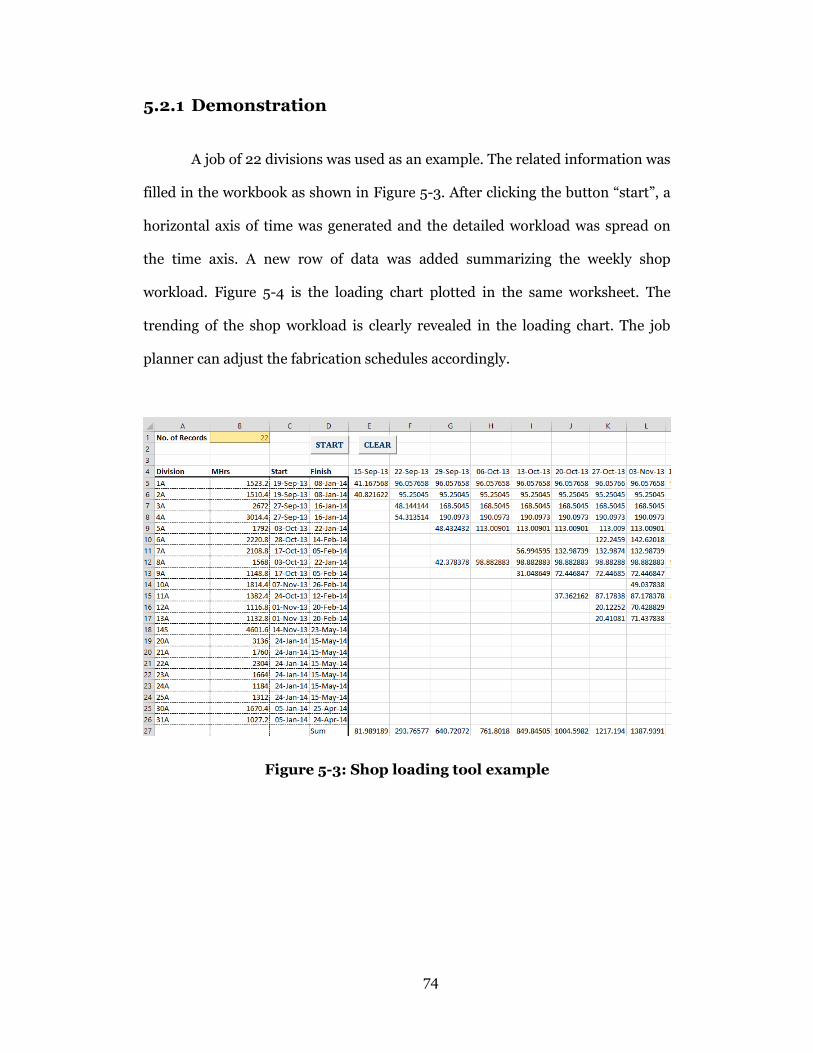
74
5.2.1 Demonstration
A job of 22 divisions was used as an example. The related information was
filled in the workbook as shown in Figure 5-3. After clicking the button “start”, a
horizontal axis of time was generated and the detailed workload was spread on
the time axis. A new row of data was added summarizing the weekly shop
workload. Figure 5-4 is the loading chart plotted in the same worksheet. The
trending of the shop workload is clearly revealed in the loading chart. The job
planner can adjust the fabrication schedules accordingly.
Figure 5-3: Shop loading tool example
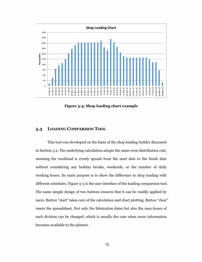
75
Figure 5-4: Shop loading chart example
5.3 LOADING COMPARISON TOOL
This tool was developed on the basis of the shop loading builder discussed
in Section 5.2. The underlying calculation adopts the same even-distribution rule,
meaning the workload is evenly spread from the start date to the finish date
without considering any holiday breaks, weekends, or the number of daily
working hours. Its main purpose is to show the difference in shop loading with
different schedules. Figure 5-5 is the user interface of the loading comparison tool.
The same simple design of two buttons ensures that it can be readily applied by
users. Button “start” takes care of the calculation and chart plotting. Button “clear”
resets the spreadsheet. Not only the fabrication dates but also the man-hours of
each division can be changed, which is usually the case when more information
becomes available to the planner.
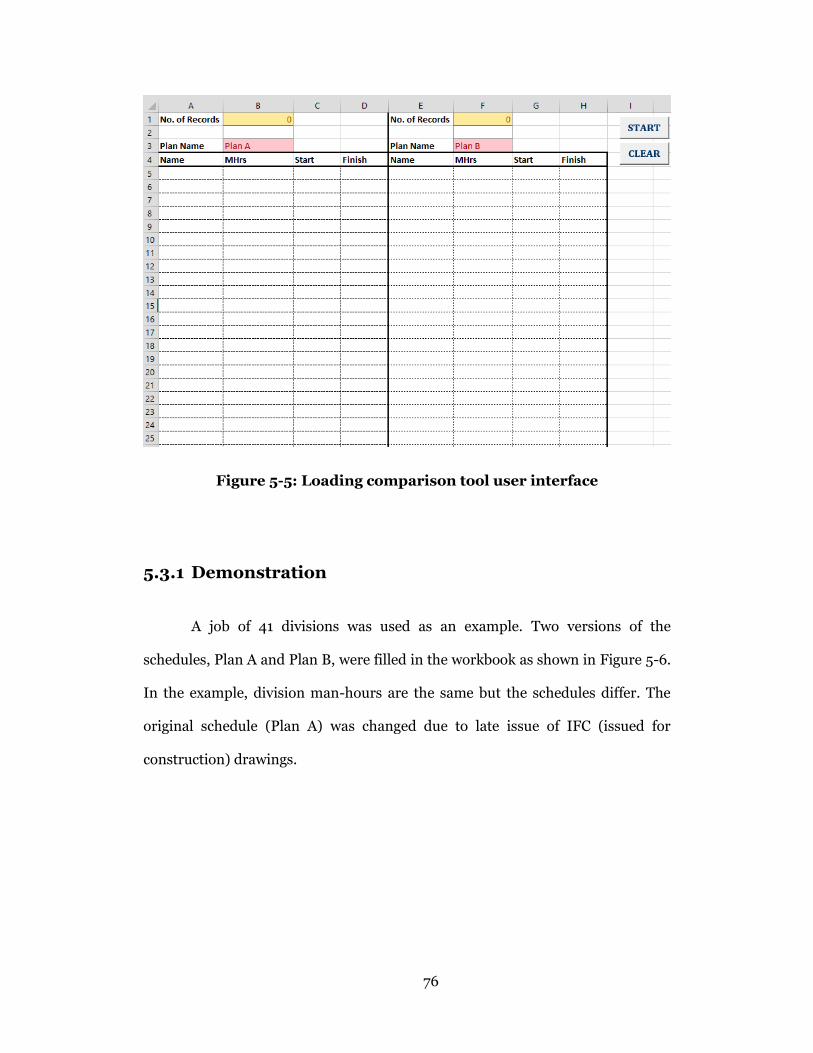
76
Figure 5-5: Loading comparison tool user interface
5.3.1 Demonstration
A job of 41 divisions was used as an example. Two versions of the
schedules, Plan A and Plan B, were filled in the workbook as shown in Figure 5-6.
In the example, division man-hours are the same but the schedules differ. The
original schedule (Plan A) was changed due to late issue of IFC (issued for
construction) drawings.
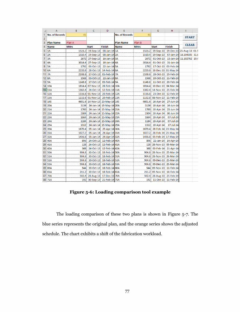
77
Figure 5-6: Loading comparison tool example
The loading comparison of these two plans is shown in Figure 5-7. The
blue series represents the original plan, and the orange series shows the adjusted
schedule. The chart exhibits a shift of the fabrication workload.
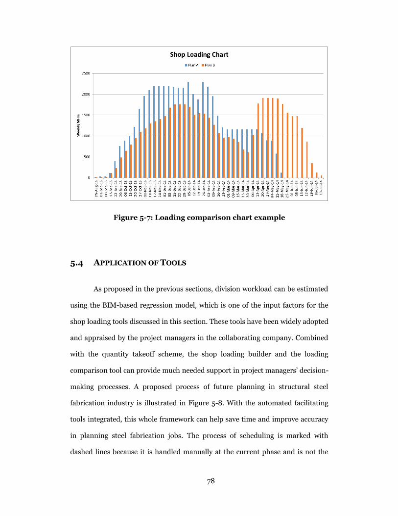
78
Figure 5-7: Loading comparison chart example
5.4 APPLICATION OF TOOLS
As proposed in the previous sections, division workload can be estimated
using the BIM-based regression model, which is one of the input factors for the
shop loading tools discussed in this section. These tools have been widely adopted
and appraised by the project managers in the collaborating company. Combined
with the quantity takeoff scheme, the shop loading builder and the loading
comparison tool can provide much needed support in project managers’ decision-
making processes. A proposed process of future planning in structural steel
fabrication industry is illustrated in Figure 5-8. With the automated facilitating
tools integrated, this whole framework can help save time and improve accuracy
in planning steel fabrication jobs. The process of scheduling is marked with
dashed lines because it is handled manually at the current phase and is not the
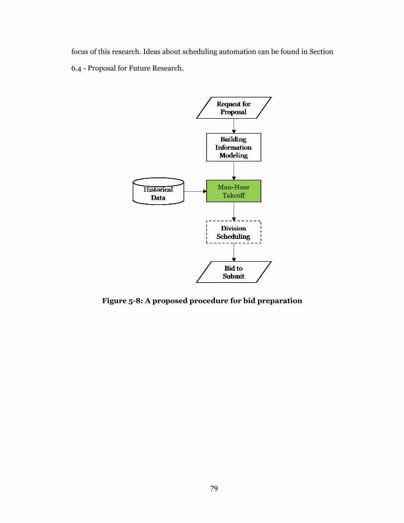
79
focus of this research. Ideas about scheduling automation can be found in Section
6.4 - Proposal for Future Research.
Figure 5-8: A proposed procedure for bid preparation
80
Chapter 6. CONCLUSIONS
6.1 SUMMARY
Structural steel fabrication is an industry with characteristics that makes
it different from traditional construction and manufacturing. The use of BIM is
on the rise not only in general construction but also in structural steel fabrication.
However, the functions and advantages of BIM-based models are limited to
design and drafting in most cases. This research aims to develop an approach to
extend BIM’s usage further into estimating and planning phases. The
performance information recorded in historical BIM data is important and can be
predictive for the company’s future projects. Expanding the scope of application
of BIM is essential to improving the efficiency of steel fabrication work in terms
of reducing implementation costs and satisfying project objectives such as
schedule milestones.
This study develops a linear regression model to provide man-hour
requirement estimate for steel fabrication projects in the planning phase. The
proposed methodology is implemented and validated, proving the models to be
both feasible and recommended to support project estimating and planning. The
models were developed using the production data from the collaborating
company, so that they were customized to the company’s information
management system (IMS). Another steel fabrication company may have
different ways of tracking data and implementing IMS, but the methodology and
framework of the study can still be used for the development of quantity take-off
prediction models.

81
Furthermore, two Excel macro-enabled workbooks were developed for the
purpose of facilitating shop operation scheduling. Used in combination with the
BIM-based quantity takeoff solution, the shop loading tools provide decision-
making support for project managers in the structural steel fabrication industry.
6.2 LIMITATIONS
Fitting and welding are generally the most complex and time-consuming
steps in steel fabrication. Different designs of the connections make a big
difference to the fitting and welding workload, affecting the overall fabrication
duration. For example, a column with end plates may be designed to be
connected using bolts only, the fabrication of which requires cutting and detailing.
This issue is another contributing factor to the regression errors observed.
This research does not take into consideration the complexity of
connections, such as the specific number of stiffeners to weld, the type of welding,
and the number of plates to bolt. The reason for this is that most of the time,
information on connections is not available during bidding. It is typically the
contractor’s duty to complement the customer’s preliminary design with detailed
connection designs, upgrading customer drawings to fabrication drawings. In
general, the time before bid submission is not enough to complete connection
design. Thus the information is normally not ready until the award of contract.
Currently structural steel fabrication shops are also sometimes
responsible for assembling the steel elements to a certain extent before shipping
to the erection site. Offsite assembly results in cost and time savings at the
erection site, and improvement of construction quality. Those steel elements are
called super-assembly or sub-assembly (SA) structures and are different from
traditional beam line type fabrication. SA demands not only additional labour but

82
also takes more time in the shop. An SA structure is generally larger than a single
piece so that extra labour and equipment is required to handle it. It also takes
time to wait for the composition pieces to be fabricated before assembly can
commence or continue. This research does not distinguish specifically the
assembly of SA structures from traditional streamlined fabrication for that the
problem definition and data collection are both on the division level. It is
appropriate to let the modeling training process in WEKA resolve the issue by
clustering structure types and factoring in extra labour hours by adjusting the
coefficients for SA structures.
6.3 RECOMMENDATIONS TO WSF
To fully utilize the results of this research, a few recommendations are
listed for WSF.
It is recommended to keep adding new data to the training dataset
and re-train the prediction model on a 3-month basis. Without
proper update, the model trained a few years ago is not likely to
work well for jobs now.
The absolute error of the modeling results can be related to a
margin estimate of the job in bidding. Questionnaires need to be
designed to obtain expert opinions on this.
To increase the prediction accuracy, jobs can be classified based on
their dimensional characteristics, before the modeling process.
The time tracking methods on the shop floor can be upgraded to
improve the quality of the man-hour data collected.

83
More data are to be collected to finalize the boundaries of the
input parameters, and set the low and high limit for the output
parameter, making the MHr prediction more reasonable.
6.4 PROPOSAL FOR FUTURE RESEARCH
The results of this study show much promise for advanced BIM in steel
fabrication planning and control. The combination of BIM with the current
scheduling and fabrication process can be investigated in future studies.
Starting from the current development, automatic scheduling on the shop
floor can be investigated. A number of issues must be addressed, including how
to determine the priority of various steel elements in scheduling, the complexity
of the specific fabrication, and optimal allocation of the various resources on the
shop floor. With the scheduling process handled by artificial intelligence, the
whole process shown in Figure 5-8 would be complete and become an integrated
system of estimating and scheduling, pushing the application of BIM further to
the planning stage in steel fabrication shops.

84
REFERENCES
Aranda-Mena, Guillermo, John Crawford, Agustin Chevez, and Thomas Froese.
2009. “Building Information Modelling Demystified: Does It Make Business
Sense to Adopt BIM?” International Journal of Managing Projects in
Business 2 (3): 419–34. doi:10.1108/17538370910971063.
Autodesk. 2003. Building Information Modeling. San Rafael, CA: Autodesk, Inc.
http://www.laiserin.com/features/bim/autodesk_bim.pdf.
Azimi, Reza, SangHyun Lee, Simaan M. AbouRizk, and Amin Alvanchi. 2011. “A
Framework for an Automated and Integrated Project Monitoring and Control
System for Steel Fabrication Projects.” Automation in Construction, Global
convergence in construction, 20 (1): 88–97. doi:10.1016/j.autcon.2010.07.001.
Berman, Gary. 2014. “STRUCTURAL STEEL DESIGN AND CONSTRUCTION -
Greyhawk.” Accessed June 18.
https://www.yumpu.com/en/document/view/4478730/structural-steel-
design-and-construction-greyhawk.
Bouckaert, Remco, Eibe Frank, Mark Hall, Richard Kirkby, Peter Reutemann,
Alex Seewald, and David Scuse. 2014. “WEKA Manual for Version 3-6-11.”
The University of Waikato.
Broomhead, D. S., and David Lowe. 1988. “Multivariable Functional
Interpolation and Adaptive Networks.” Complex Systems 2 (3): 321–55.
Brownlee, Jason. 2013a. “A Tour of Machine Learning Algorithms | Machine
Learning Mastery.” Machine Learning Mastery. November 25.
http://machinelearningmastery.com/a-tour-of-machine-learning-algorithms.
———. 2013b. “How to Prepare Data For Machine Learning | Machine Learning
Mastery.” Machine Learning Mastery. December 25.
http://machinelearningmastery.com/how-to-prepare-data-for-machine-
learning/.
buildingSMART. 2014. “Industry Foundation Classes (IFC) Data Model —
buildingSMART.” Accessed June 24.
http://www.buildingsmart.org/standards/ifc.
85
Burnham, Kenneth P., and David R. Anderson. 2002. Model Selection and
Multimodel Inference: A Practical Information-Theoretic Approach.
Springer.
Chiu, Chui-Te, Tseng-Hsing Hsu, Ming-Teh Wang, and Hsien-Yen Chiu. 2011.
“Simulation for Steel Bridge Erection by Using BIM Tools.” Proceedings of
the 28th ISARC, Seoul, Korea, 560–63.
CII. 1995. Pre-Project Planning Handbook. Special Publication 39-2. University
of Texas at Austin. https://www.construction-
institute.org/scriptcontent/more/sp39_2_more.cfm.
Cortes, Corinna, and Vladimir Vapnik. 1995. “Support-Vector Networks.”
Machine Learning 20 (3): 273–97. doi:10.1007/BF00994018.
Cover, T.M. 1965. “Geometrical and Statistical Properties of Systems of Linear
Inequalities with Applications in Pattern Recognition.” IEEE Transactions on
Electronic Computers EC-14 (3): 326–34. doi:10.1109/PGEC.1965.264137.
Cross Validated. 2011. “Understanding SVM Regression: Objective Function and
‘Flatness.’” Q&A site. Cross Validated. January.
http://stats.stackexchange.com/questions/5945/understanding-svm-
regression-objective-function-and-flatness.
———. 2013. “What Is the Difference between Data Mining, Statistics, Machine
Learning and AI?” Q&A site. Cross Validated.
http://stats.stackexchange.com/questions/5026/what-is-the-difference-
between-data-mining-statistics-machine-learning-and-ai.
Dozzi, S. P., and Simaan M. AbouRizk. 1993. Productivity in Construction.
National Research Council Canada. http://archive.nrc-
cnrc.gc.ca/obj/irc/doc/pubs/nrcc37001.pdf.
Eastman, Chuck. 2006. IFC Overview. Georgia Tech. https://open-acad-
lib.googlecode.com/files/%E3%80%8ABIM%2BHandbook%E3%80%8B%E5
%AF%B9IFC%E7%9A%84%E4%BB%8B%E7%BB%8D.pdf.
Eastman, Chuck, and R. Sacks. 2008. “Relative Productivity in the AEC
Industries in the United States for On-Site and Off-Site Activities.” Journal of
Construction Engineering and Management 134 (7): 517–26.
doi:10.1061/(ASCE)0733-9364(2008)134:7(517).
El-Abbasy, M., A. Senouci, T. Zayed, F. Mirahadi, and L. Parvizsedghy. 2014.
“Condition Prediction Models for Oil and Gas Pipelines Using Regression

86
Analysis.” Journal of Construction Engineering and Management 0 (0):
04014013. doi:10.1061/(ASCE)CO.1943-7862.0000838.
Fayek, A., and A. Oduba. 2005. “Predicting Industrial Construction Labor
Productivity Using Fuzzy Expert Systems.” Journal of Construction
Engineering and Management 131 (8): 938–41. doi:10.1061/(ASCE)0733-
9364(2005)131:8(938).
Flake, Gary William, and Steve Lawrence. 2002. “Efficient SVM Regression
Training with SMO.” Machine Learning 46 (1-3): 271–90.
doi:10.1023/A:1012474916001.
Hall, Mark, Eibe Frank, Geoffrey Holmes, Bernhard Pfahringer, Peter
Reutemann, and Ian H. Witten. 2009. “The WEKA Data Mining Software: An
Update.” SIGKDD Explorations 11 (1).
Haykin, Simon S. 1999. Neural Networks: A Comprehensive Foundation.
Prentice Hall.
Hergunsel, Mehmet F. 2011. “Benefits of Building Information Modeling for
Construction Managers and BIM Based Scheduling.” Worcester Polytechnic
Institute. https://www.wpi.edu/Pubs/ETD/Available/etd-042011-
135239/unrestricted/MHergunsel_Thesis_BIM.pdf.
Howard, Rob, and Bo-Christer Björk. 2008. “Building Information Modelling –
Experts’ Views on Standardisation and Industry Deployment.” Advanced
Engineering Informatics, Network methods in engineering, 22 (2): 271–80.
doi:10.1016/j.aei.2007.03.001.
Hu, Di, and Yasser Mohamed. 2012. “Automating Fabrication Sequencing for
Industrial Construction.” Gerontechnology 11 (2).
doi:10.4017/gt.2012.11.02.318.749.
Ikerd, W. F. 2008. “The Importance of BIM in Structural Engineering.” Structure
Magazine. http://www.structuremag.org/Archives/2008-10/C-Technology-
Ikerd-Oct08.pdf.
Jung, Youngsoo, and Mihee Joo. 2011. “Building Information Modelling (BIM)
Framework for Practical Implementation.” Automation in Construction 20
(2): 126–33. doi:10.1016/j.autcon.2010.09.010.
Kalavagunta, Sreedhar. 2012. “Integrated Engineering Workflow (BIM) for
Design of Steel Structures.” In Australasian Structural Engineering
87
Conference 2012: The Past, Present and Future of Structural Engineering,
498. http://asec2012.conference.net.au/papers/063.pdf.
Karshenas, Saeed, and Xin Feng. 1992. “Application of Neural Networks in
Earthmoving Equipment Production Estimating.” In Computing in Civil
Engineering and Geographic Information Systems Symposium, 841–47.
ASCE. http://cedb.asce.org/cgi/WWWdisplay.cgi?9201884.
Lancaster, F., and J. Tobin. 2013. “Integrated Project Delivery: Next-Generation
BIM for Structural Engineering.” In Structures Congress 2010, 2809–18.
American Society of Civil Engineers. Accessed November 18.
http://ascelibrary.org/doi/abs/10.1061/41130%28369%29254.
Lee, Jong-Kyun, Boo-Young Kim, Jang-Young Kim, Tae-Hui Kim, and Kiyoung
Son. 2013. “A Quantity Prediction Model for Reinforced Concrete and Bricks
in Education Facilities Using Regression Analysis.” Journal of the Korea
Institute of Building Construction 13 (5): 506–12.
doi:10.5345/JKIBC.2013.13.5.506.
Lu, Ming. 2001. “Productivity Studies Using Advanced ANN Models.” Ph.D.
thesis, Edmonton, Alberta.: University of Alberta.
http://www.collectionscanada.gc.ca/obj/s4/f2/dsk1/tape4/PQDD_0012/NQ
60322.pdf.
Mitchell, Tom M. 1997. Machine Learning. 1 edition. New York: McGraw-Hill
Science/Engineering/Math.
Monteiro, André, and João Poças Martins. 2013. “A Survey on Modeling
Guidelines for Quantity Takeoff-Oriented BIM-Based Design.” Automation in
Construction 35 (November): 238–53. doi:10.1016/j.autcon.2013.05.005.
National Building Information Model Standard Project Committee. 2014. “What
Is a BIM?” National BIM Standard - United States. Accessed April 29.
http://www.nationalbimstandard.org/faq.php#faq1.
Nawari, N. 2012. “BIM Standard in Off-Site Construction.” Journal of
Architectural Engineering 18 (2): 107–13. doi:10.1061/(ASCE)AE.1943-
5568.0000056.
Peterson, Forest, Timo Hartmann, Renate Fruchter, and Martin Fischer. 2011.
“Teaching Construction Project Management with BIM Support: Experience
and Lessons Learned.” Automation in Construction 20 (2): 115–25.
doi:10.1016/j.autcon.2010.09.009.
88
Platt, John C. 1998. Sequential Minimal Optimization: A Fast Algorithm for
Training Support Vector Machines. Technical Report. MSR-TR-98-14.
Microsoft Research.
Portas, Jason B. 1996. “Estimating Concrete Formwork Productivity.” Master of
Science, University of Alberta.
ResearchGate. 2013. “What Is the Difference between Machine Learning and
Data Mining ?” Professional network. ResearchGate.
http://www.researchgate.net/post/What_is_the_difference_between_machi
ne_learning_and_data_mining.
Sattineni, Anoop, and R. Harrison Bradford. 2011. “Estimating with BIM: A
Survey of US Construction Companies.” Proceedings of the 28th
International Symposium on Automation and Robotics in Construction,
564–69.
Shevade, S.K., S.S. Keerthi, C. Bhattacharyya, and K. R K Murthy. 2000.
“Improvements to the SMO Algorithm for SVM Regression.” IEEE
Transactions on Neural Networks 11 (5): 1188–93. doi:10.1109/72.870050.
Shi, Wei. 2009. “Framework for Integration of BIM and RFID in Steel
Construction.” University of Florida.
http://purl.fcla.edu/fcla/etd/UFE0041169.
Simon, Phil. 2013. Too Big to Ignore: The Business Case for Big Data. Hoboken,
New Jersey: Wiley.
Smith, S. 1999. “Earthmoving Productivity Estimation Using Linear Regression
Techniques.” Journal of Construction Engineering and Management 125 (3):
133–41. doi:10.1061/(ASCE)0733-9364(1999)125:3(133).
Smola, Alex J., and Bernhard Schölkopf. 2004. “A Tutorial on Support Vector
Regression.” Statistics and Computing 14 (3): 199–222.
doi:10.1023/B:STCO.0000035301.49549.88.
Song, Lingguang, and Simaan M. AbouRizk. 2008. “Measuring and Modeling
Labor Productivity Using Historical Data.” Journal of Construction
Engineering and Management 134 (10): 786–94. doi:10.1061/(ASCE)0733-
9364(2008)134:10(786).
Sonmez, R., and J. Rowings. 1998. “Construction Labor Productivity Modeling
with Neural Networks.” Journal of Construction Engineering and

89
Management 124 (6): 498–504. doi:10.1061/(ASCE)0733-
9364(1998)124:6(498).
SteelConstruction.info. 2014. “The Case for Steel.” Steelconstruction.info.
Accessed April 27. http://www.steelconstruction.info/The_case_for_steel.
Steel, Jim, Robin Drogemuller, and Bianca Toth. 2012. “Model Interoperability in
Building Information Modelling.” Software & Systems Modeling 11 (1): 99–
109. doi:10.1007/s10270-010-0178-4.
“Support Vector Machine Regression.” 2014. Support Vector Machine
Regression. Accessed July 22. http://kernelsvm.tripod.com/.
Tekla. 2014a. “Tekla.” Tekla. Accessed April 30. http://www.tekla.com/us.
———. 2014b. “Structural Steel Detailing and Fabrication Software | Tekla.” Tekla.
Accessed June 24. http://www.tekla.com/solutions/steel-fabricators.
The University of Waikato. 2014. “Weka 3 - Data Mining with Open Source
Machine Learning Software in Java.” WEKA. Accessed April 30.
http://www.cs.waikato.ac.nz/ml/weka/.
Tiwari, Saurabh, Josh Odelson, Alan Watt, and Atul Khanzode. 2009. “Model
Based Estimating to Inform Target Value Design.” AECbytes “Building the
Future” Article.
http://www.aecbytes.com/buildingthefuture/2009/ModelBasedEstimating.h
tml.
Vertigraph Inc. 2004. “Automating the Takeoff and Estimating Process.”
www.vertigraph.com.
Whitt, Michael. 2012. Successful Instrumentation and Control Systems Design.
2nd edition. Research Triangle Park, NC: ISA - The Instrumentation, Systems
& Automation Society.
Williams, Alan. 2011. Steel Structures Design: ASD/LRFD. 1 edition. New York:
McGraw-Hill Professional.
Witten, Ian H., Eibe Frank, and Mark A. Hall. 2011. Data Mining: Practical
Machine Learning Tools and Techniques, Third Edition. 3 edition.
Burlington, MA: Morgan Kaufmann.
Xie, Haiyan, Wei Shi, and Raja RA Issa. 2010. “Implementation of BIM/RFID in
Computer-Aided Design-Manufacturing-Installation Process.” In Computer
Science and Information Technology (ICCSIT), 2010 3rd IEEE International

90
Conference on, 2:107–11.
http://ieeexplore.ieee.org/xpls/abs_all.jsp?arnumber=5563653.

91
APPENDIX A: SHOP LOADING TOOL MACRO CODE
Module 1:
Sub ButtonStart_Click()
Dim shopSheet As Worksheet
Set shopSheet = ThisWorkbook.ActiveSheet
Call SpreadWork(shopSheet, shopSheet.Name)
End Sub
Sub ButtonClear_Click()
Dim shopSheet As Worksheet
Set shopSheet = ThisWorkbook.ActiveSheet
Call ClearSheet(shopSheet)
End Sub
Module 2:
' Clear all the data of Row 4 and below.
Sub ClearSheet(ByRef mysh As Worksheet)
mysh.Rows("4:" & mysh.Rows.Count).ClearContents
' Write the column titles back.
mysh.Cells(4, 1).Value = "Name"
mysh.Cells(4, 2).Value = "MHrs"
mysh.Cells(4, 3).Value = "Start"
mysh.Cells(4, 4).Value = "Finish"
' Reset the formula in cell B1
mysh.Cells(1, 2).Formula = "=COUNTA(A:A)-2"
Dim chartObj As ChartObject

92
For Each chartObj In mysh.ChartObjects
chartObj.Delete
Next
End Sub
Sub SpreadWork(ByRef mysh As Worksheet, ByVal chtName As
String)
If mysh.Range("B1").Value = "" Or mysh.Range("B1").Value
= 0 Then
Call MsgBox("Please enter the Number of Records.",
vbOKOnly, "CAUTION!")
Exit Sub
End If
Dim numOfRecords As Integer
numOfRecords = mysh.Range("B1").Value
Dim wkRow As Integer
Dim wkCol As Integer
wkRow = 4 ' Row number 4
wkCol = 5 ' Column E
Dim minStart As Date
Dim maxFinish As Date
minStart = WorksheetFunction.min(mysh.Range("C" & (wkRow
+ 1) & ":C" & (wkRow + numOfRecords)))

93
maxFinish = WorksheetFunction.Max(mysh.Range("D" &
(wkRow + 1) & ":D" & (wkRow + numOfRecords)))
Dim minSun As Date
Dim maxSun As Date
minSun = FirstDayofWeek(minStart)
maxSun = FirstDayofWeek(maxFinish)
mysh.Cells(wkRow, wkCol).Select ' Select the start point
of the timeline axis.
Dim axisDate As Date
axisDate = minSun
' Create the horizontal time axis.
Do
Selection.Value = axisDate
Selection.NumberFormat = "dd-mmm-yy"
Selection.Offset(0, 1).Select ' Move right by one
cell.
axisDate = axisDate + 7
Loop While axisDate <= maxSun
' Clear all the cell contents.
Dim colMax As String
colMax = ColumnLetter(Selection.Column - 1)
Dim wkColName As String
wkColName = ColumnLetter(wkCol)

94
mysh.Range(wkColName & (wkRow + 1) & ":" & colMax &
(wkRow + numOfRecords + 1)).ClearContents
Dim counter As Integer
For counter = 1 To numOfRecords
Dim taskStart As Date
Dim taskFinish As Date
taskStart = mysh.Range("C" & (wkRow +
counter)).Value
taskFinish = mysh.Range("D" & (wkRow +
counter)).Value
' Check
If taskStart > taskFinish Then
Call MsgBox("Start Date is later than Finish
Date on line " & (wkRow + counter) & ".", vbOKOnly,
"CAUTION!")
Exit Sub
End If
Dim avgMh As Double
avgMh = mysh.Range("B" & (wkRow + counter)).Value /
(taskFinish - taskStart)
Dim firstWk As Date
Dim lastWk As Date
firstWk = FirstDayofWeek(taskStart)
lastWk = FirstDayofWeek(taskFinish)

95
mysh.Cells(wkRow, wkCol).Select
' Set workload of the first week
Do While Selection.Value < firstWk
Selection.Offset(0, 1).Select
Loop
mysh.Cells((wkRow + counter),
Selection.Column).Value = avgMh * (Selection.Value + 7 -
taskStart)
' Set workload in the middle week(s)
Selection.Offset(0, 1).Select
Do While Selection.Value < lastWk
mysh.Cells((wkRow + counter),
Selection.Column).Value = avgMh * 7
Selection.Offset(0, 1).Select
Loop
' Set workload of the last week
mysh.Cells((wkRow + counter),
Selection.Column).Value = avgMh * (taskFinish -
Selection.Value)
Next counter
mysh.Cells(wkRow + numOfRecords + 1, wkCol - 1).Value =
"Sum"
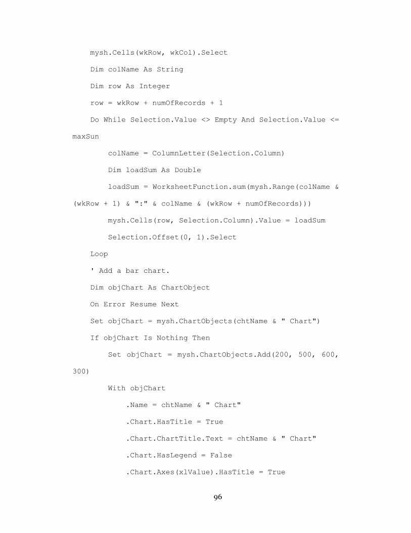
96
mysh.Cells(wkRow, wkCol).Select
Dim colName As String
Dim row As Integer
row = wkRow + numOfRecords + 1
Do While Selection.Value <> Empty And Selection.Value <=
maxSun
colName = ColumnLetter(Selection.Column)
Dim loadSum As Double
loadSum = WorksheetFunction.sum(mysh.Range(colName &
(wkRow + 1) & ":" & colName & (wkRow + numOfRecords)))
mysh.Cells(row, Selection.Column).Value = loadSum
Selection.Offset(0, 1).Select
Loop
' Add a bar chart.
Dim objChart As ChartObject
On Error Resume Next
Set objChart = mysh.ChartObjects(chtName & " Chart")
If objChart Is Nothing Then
Set objChart = mysh.ChartObjects.Add(200, 500, 600,
300)
With objChart
.Name = chtName & " Chart"
.Chart.HasTitle = True
.Chart.ChartTitle.Text = chtName & " Chart"
.Chart.HasLegend = False
.Chart.Axes(xlValue).HasTitle = True
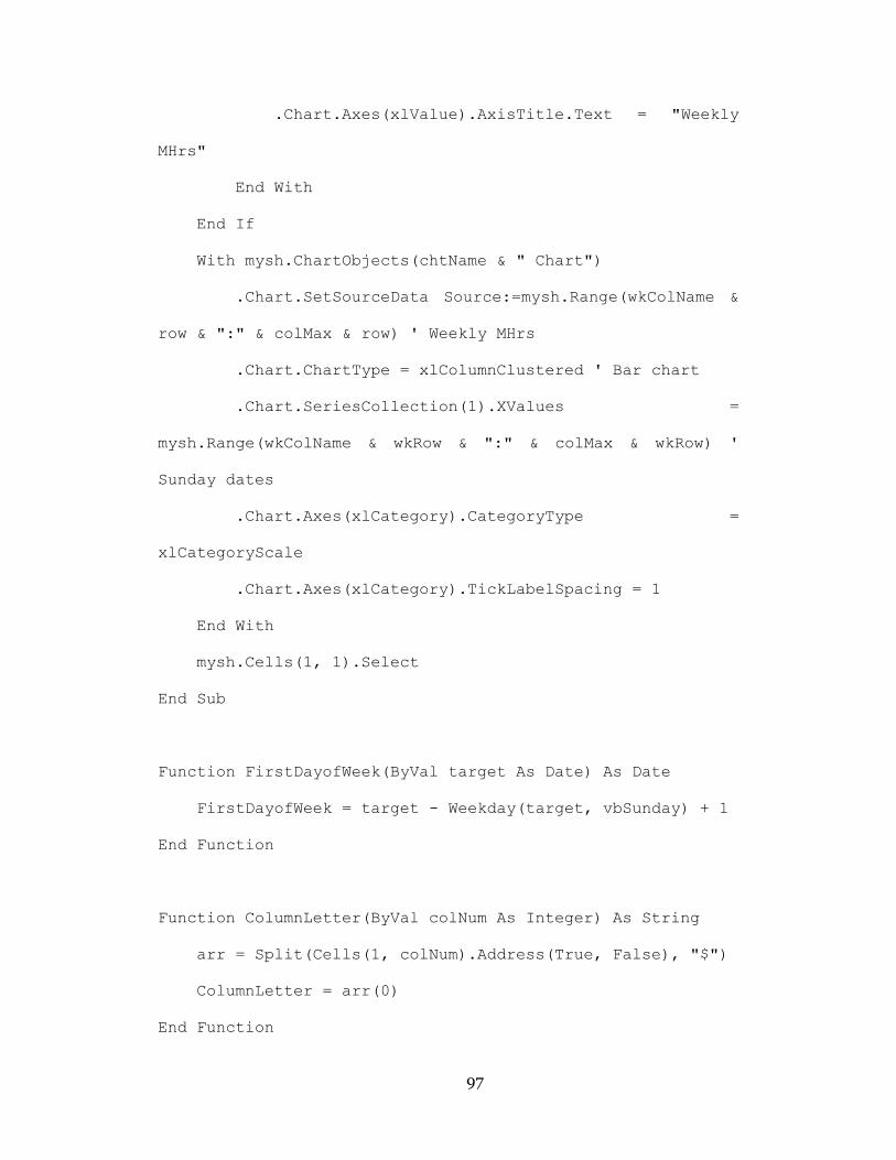
97
.Chart.Axes(xlValue).AxisTitle.Text = "Weekly
MHrs"
End With
End If
With mysh.ChartObjects(chtName & " Chart")
.Chart.SetSourceData Source:=mysh.Range(wkColName &
row & ":" & colMax & row) ' Weekly MHrs
.Chart.ChartType = xlColumnClustered ' Bar chart
.Chart.SeriesCollection(1).XValues =
mysh.Range(wkColName & wkRow & ":" & colMax & wkRow) '
Sunday dates
.Chart.Axes(xlCategory).CategoryType =
xlCategoryScale
.Chart.Axes(xlCategory).TickLabelSpacing = 1
End With
mysh.Cells(1, 1).Select
End Sub
Function FirstDayofWeek(ByVal target As Date) As Date
FirstDayofWeek = target - Weekday(target, vbSunday) + 1
End Function
Function ColumnLetter(ByVal colNum As Integer) As String
arr = Split(Cells(1, colNum).Address(True, False), "$")
ColumnLetter = arr(0)
End Function

98
APPENDIX B: LOADING COMPARISON TOOL MACRO
CODE
Module 1:
Sub ButtonStart_Click()
Dim shopSheet As Worksheet
Set shopSheet = ThisWorkbook.ActiveSheet
Call SpreadWork(shopSheet)
End Sub
Sub ButtonClear_Click()
Dim shopSheet As Worksheet
Set shopSheet = ThisWorkbook.ActiveSheet
Call ClearSheet(shopSheet)
End Sub
Module 2:
Option Explicit
' Clear all the data below the column title at Row 4.
Sub ClearSheet(ByRef mysh As Worksheet)
mysh.Rows("5:" & mysh.Rows.Count).ClearContents
' Reset the formula in cell B1 and F1
mysh.Cells(1, 2).Formula = "=COUNTA(A:A)-3"
mysh.Cells(1, 6).Formula = "=COUNTA(E:E)-3"

99
Dim chartObj As ChartObject
For Each chartObj In mysh.ChartObjects
chartObj.Delete
Next
End Sub
Sub SpreadWork(ByRef mysh As Worksheet)
If mysh.Range("B1").value = "" Or mysh.Range("B1").value
= 0 Then
Call MsgBox("Please enter the Number of Records and
MHrs per Tonne.", vbOKOnly, "CAUTION!")
Exit Sub
End If
Dim ConsWkRow As Integer ' Two constants
Dim ConsWkCol As Integer
ConsWkRow = 5 ' Row number 5, the row below the column
titles.
ConsWkCol = 9 ' Column I
'''' Schedule A ''''
Dim numOfRecords As Integer
numOfRecords = mysh.Range("B1").value
Dim minStart As Date
Dim maxFinish As Date

100
minStart = WorksheetFunction.min(mysh.Range("C" &
ConsWkRow & ":C" & (ConsWkRow + numOfRecords - 1)))
maxFinish = WorksheetFunction.Max(mysh.Range("D" &
ConsWkRow & ":D" & (ConsWkRow + numOfRecords - 1)))
Dim minSun As Date ' Start and end of the timeline
Dim maxSun As Date
minSun = FirstDayofWeek(minStart)
maxSun = FirstDayofWeek(maxFinish)
Dim wkLoading As Collection
Set wkLoading = New Collection
Dim axisDate As Date
axisDate = minSun
' Create the horizontal time axis.
Dim tmp As ClsWkLoad
Do
Set tmp = New ClsWkLoad
tmp.Init axisDate
wkLoading.Add tmp
axisDate = axisDate + 7
Loop While axisDate <= maxSun
''' Main Calculation '''
Dim counter As Integer
For counter = 1 To numOfRecords
Dim taskStart As Date

101
Dim taskFinish As Date
taskStart = mysh.Range("C" & (ConsWkRow + counter -
1)).value
taskFinish = mysh.Range("D" & (ConsWkRow + counter -
1)).value
' Check
If taskStart > taskFinish Then
Call MsgBox("Start Date is later than Finish
Date on line " & (ConsWkRow + counter - 1) & ".", vbOKOnly,
"CAUTION!")
Exit Sub
End If
Dim avgMh As Double
avgMh = mysh.Range("B" & (ConsWkRow + counter -
1)).value / (taskFinish - taskStart) ' Daily average Mhrs
Dim firstWk As Date
Dim lastWk As Date
firstWk = FirstDayofWeek(taskStart)
lastWk = FirstDayofWeek(taskFinish)
Dim firstIdx As Integer ' Index in the collection
Dim lastIdx As Integer
firstIdx = (firstWk - wkLoading.Item(1).Week) / 7 +
1
lastIdx = (lastWk - wkLoading.Item(1).Week) / 7 + 1
102
wkLoading.Item(firstIdx).AddHr avgMh * (firstWk + 7
- taskStart), 1
Dim index As Integer
For index = firstIdx + 1 To lastIdx - 1
wkLoading.Item(index).AddHr avgMh * 7, 1
Next index
wkLoading.Item(lastIdx).AddHr avgMh * (taskFinish -
lastWk), 1
Next counter
'''' Schedule B ''''
numOfRecords = mysh.Range("F1").value
If numOfRecords > 0 Then
minStart = WorksheetFunction.min(mysh.Range("G" &
ConsWkRow & ":G" & (ConsWkRow + numOfRecords - 1)))
maxFinish = WorksheetFunction.Max(mysh.Range("H" &
ConsWkRow & ":H" & (ConsWkRow + numOfRecords - 1)))
minSun = FirstDayofWeek(minStart) ' Start and end of
the timeline
maxSun = FirstDayofWeek(maxFinish)
axisDate = wkLoading.Item(1).Week ' The first date
on the current time axis
Do While axisDate > minSun ' The axis is not enough.
103
axisDate = axisDate - 7
Set tmp = New ClsWkLoad
tmp.Init axisDate
wkLoading.Add tmp, , 1 ' Insert in the beginning
Loop
axisDate = wkLoading.Item(wkLoading.Count).Week
Do While axisDate < maxSun
axisDate = axisDate + 7
Set tmp = New ClsWkLoad
tmp.Init axisDate
wkLoading.Add tmp, , , wkLoading.Count ' Insert
to the end
Loop
''' Main Calculation '''
For counter = 1 To numOfRecords
taskStart = mysh.Range("G" & (ConsWkRow +
counter - 1)).value
taskFinish = mysh.Range("H" & (ConsWkRow +
counter - 1)).value
' Check
If taskStart > taskFinish Then
Call MsgBox("Start Date is later than Finish
Date on line " & (ConsWkRow + counter - 1) & ".", vbOKOnly,
"CAUTION!")
Exit Sub
104
End If
avgMh = mysh.Range("F" & (ConsWkRow + counter -
1)).value / (taskFinish - taskStart) ' Daily average Mhrs
firstWk = FirstDayofWeek(taskStart)
lastWk = FirstDayofWeek(taskFinish)
firstIdx = (firstWk - wkLoading.Item(1).Week) /
7 + 1
lastIdx = (lastWk - wkLoading.Item(1).Week) / 7
+ 1
wkLoading.Item(firstIdx).AddHr avgMh * (firstWk
+ 7 - taskStart), 2
For index = firstIdx + 1 To lastIdx - 1
wkLoading.Item(index).AddHr avgMh * 7, 2
Next index
wkLoading.Item(lastIdx).AddHr avgMh *
(taskFinish - lastWk), 2
Next counter
End If
''' Fill the weekly summary in the spreadsheet. '''
mysh.Cells(ConsWkRow, ConsWkCol).Select ' Start of the
timeline axis
For counter = 1 To wkLoading.Count
Selection.value = wkLoading.Item(counter).Week
105
Selection.NumberFormat = "dd-mmm-yy"
Selection.Offset(1, 0).value =
wkLoading.Item(counter).MhrA
Selection.Offset(2, 0).value =
wkLoading.Item(counter).MhrB
Selection.Offset(0, 1).Select ' Move right.
Next counter
Dim colMax As String
colMax = ColumnLetter(Selection.Column - 1)
Dim xSeries As String
Dim y1Series As String
Dim y2Series As String
Dim y1Name As String
Dim y2Name As String
xSeries = ColumnLetter(ConsWkCol) & ConsWkRow & ":" &
colMax & ConsWkRow
y1Name = mysh.Range("B3").value
y2Name = mysh.Range("F3").value
y1Series = ColumnLetter(ConsWkCol) & (ConsWkRow + 1) &
":" & colMax & (ConsWkRow + 1)
y2Series = ColumnLetter(ConsWkCol) & (ConsWkRow + 2) &
":" & colMax & (ConsWkRow + 2)
Call DrawChart(mysh, mysh.Name, y1Name, xSeries,
y1Series)

106
Call DrawChart(mysh, mysh.Name, y2Name, xSeries,
y2Series)
Set wkLoading = Nothing
mysh.Cells(1, 1).Select
End Sub
' Find the nearest Sunday before target, which represents
the first day of the week Target belongs to.
Function FirstDayofWeek(ByVal target As Date) As Date
FirstDayofWeek = target - Weekday(target, vbSunday) + 1
End Function
' Conver a column to a letter.
Function ColumnLetter(ByVal colNum As Integer) As String
Dim arr() As String
arr = Split(Cells(1, colNum).Address(True, False), "$")
ColumnLetter = arr(0)
End Function
' Create a bar chart.
Sub DrawChart(ByRef mysh As Worksheet, ByVal chtName As
String, ByVal seName As String, ByVal xSeries As String,
ByVal ySeries As String)
Dim objChart As ChartObject
On Error Resume Next
107
Set objChart = mysh.ChartObjects(chtName & " Chart")
If objChart Is Nothing Then ' Create if not exist
Set objChart = mysh.ChartObjects.Add(200, 500, 600,
300)
With objChart
.Name = chtName & " Chart"
.Chart.HasTitle = True
.Chart.ChartTitle.Text = chtName & " Chart"
.Chart.HasLegend = True
.Chart.Legend.Position = xlLegendPositionTop
.Chart.Axes(xlValue).HasTitle = True
.Chart.Axes(xlValue).AxisTitle.Text = "Weekly
MHrs"
End With
End If
With mysh.ChartObjects(chtName & " Chart")
With .Chart.SeriesCollection.NewSeries
.XValues = mysh.Range(xSeries) ' Sunday dates
.Values = mysh.Range(ySeries) ' Weekly MHrs
.Name = seName
End With
.Chart.ChartType = xlColumnClustered ' Bar chart
.Chart.Axes(xlCategory).CategoryType =
xlCategoryScale
.Chart.Axes(xlCategory).TickLabelSpacing = 1

108
End With
End Sub
Class Module:
Option Explicit
Private pWeek As Date
Private pMhrA As Double
Private pMhrB As Double
Public Property Get Week() As Date
Week = pWeek
End Property
Public Property Get MhrA() As Double
MhrA = pMhrA
End Property
Public Property Let MhrA(value As Double)
If value < 0 Then
pMhrA = 0
Else
pMhrA = value
End If
End Property
Public Property Get MhrB() As Double
109
MhrB = pMhrB
End Property
Public Property Let MhrB(value As Double)
If value < 0 Then
pMhrB = 0
Else
pMhrB = value
End If
End Property
Public Sub Init(value As Date)
pWeek = value
pMhrA = 0
pMhrB = 0
End Sub
Public Sub AddHr(value As Double, setNo As Integer)
If setNo = 1 Then
pMhrA = pMhrA + value
Else
pMhrB = pMhrB + value
End If
End Sub