Bill Campbell and Liz Satterfield

13th JCSDA Technical Review Meeting and Science Workshop on Satellite Data Assimilation

15 May 2015

Accounting for Correlated Satellite Observation Error in NAVGEM

1

2

Sources of Observation Error

IMPERFECTOBSERVATIONS

True Temperature in Model Space

T=28° T=38° T=58°

T=30° T=44° T=61°

T=32° T=53° T=63°

T=44°

1) Instrument error (usually, but not always, uncorrelated)2) Mapping operator (H) error (interpolation, radiative transfer)3) Pre-processing, quality control, and bias correction errors4) Error of representation (sampling or scaling error), which can

lead to correlated error:

3

Correlated Error in Operational DA

• Until recently, most operation DA systems assumed no correlations between observations at different levels or locations (i.e., a diagonal R)

• To compensate for observation errors that are actually correlated, one or more of the following is typically done:– Discard (“thin”) observations until the remaining ones are

uncorrelated (Bergman and Bonner (1976), Liu and Rabier (2003))– Local averaging (“superobbing”) (Berger and Forsythe (2004))– Inflate the observation error variances (Stewart et al. (2008, 2013)

• Theoretical studies (e.g. Stewart et al., 2009) indicate that including even approximate correlation structures outperforms diagonal R with variance inflation

• *In January, 2013, the Met Office went operational with a vertical observation error covariance submatrix for the IASI instrument, which showed forecast benefit in seasonal testing in both hemispheres (Weston et al. (2014))

4

• From O-F, O-A, and A-F statistics from any model (e.g. NAVGEM), the observation error covariance matrix R, the representer HBHT, and their sum can be diagnosed

• This method is sensitive to the R and HBHT that is prescribed in the DA system

• An iterative approach may be necessary• Diagnose R1 , which will be different from the original R • Symmetrize R1 , possibly adjusting its eigenvalue spectrum• Implement R1 and run NAVGEM • Diagnose R2 , which we hope will be closer to Rtrue

Desroziers Method(Desroziers et al. 2005)

4DVar Primal Formulation

1

11 1 1 1

1 1 1

T Tf f

T T T Tf

T Tf

w x x BH HBH R y H x

B H R H w B H R H BH HBH R y H x

B H R H w H R y H x

Scale by B-1/21 2

1 2

s B w

w B s

1 2 1 1 1 2 1 2 1

1 2 1 1 2 1 2 1

T Tf

T Tf

B B H R H B s B H R y H x

I B H R HB s B H R y H x

4D-var iteration is on this problem -- We need to invert R!

4DVar Dual Formulation

Scale by R-1/2

1/2 1/2

,{ }i j

R R

R

R C

diag

C 4D-Var iteration is on this problem – No need to invert C!

Iteration is done on partial step and then mapped back with BHT

• An advantage of the dual formulation is that correlated observation error can be implemented directly

• No matrix inverse is required, which lifts some restrictions on the feasible size of a non-diagonal R

• In particular, implementing horizontally correlated observation error is significantly less challenging

7

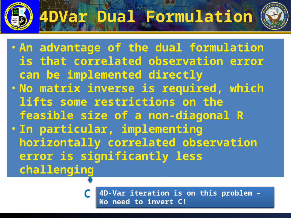
Correlated Observation Errorand the ATMS

Advanced Technology Microwave Sounder (ATMS)

13 temperature channels9 moisture channels

Channel Number

Cha

nnel

Num

ber

4 5 6 7 8 9 10 11 12 13 14 15 18 19 20 21 22

22

21

20

19

18

15

14

13

12

11

10

9

8

7

6

5

40

0.1

0.2

0.3

0.4

0.5

0.6

0.7

0.8

0.9

1

Current observation error correlation matrix used for ATMS,

and for ALL observations

8

Error Covariance Estimationfor the ATMS

Statistical Estimate

Chan

nel N

umbe

r

4 5 6 7 8 9 10 11 12 13 14 15 18 19 20 21 22 Channel Number

1.0

0.9

0.8

0.7

0.6

0.5

0.4

0.3

0.2

0.1

0.0 4

5

6

7 8

9

10

11

12 1

3 1

4 15

18

19

20

21

22

Desroziers’ method estimate of interchannel portion of observation

error correlation matrix for ATMS

1.0

0.9

0.8

0.7

0.6

0.5

0.4

0.3

0.2

0.1

0.0 4

5

6

7

8 9

10

11

12 1

3 14

15

18 1

9 20

21

22 4 5 6 7 8 9 10 11 12 13 14 15 18 19 20 21 22

Chan

nel N

umbe

r

Current Treatment

Channel Number

Temperature Temperature

Moisture Moisture

Current observation error correlation matrix used for ATMS,

and for ALL observations

9

Iterating Desroziers

Old Statistical Estimate

Chan

nel N

umbe

r

4 5 6 7 8 9 10 11 12 13 14 15 18 19 20 21 22 Channel Number

1.0

0.9

0.8

0.7

0.6

0.5

0.4

0.3

0.2

0.1

0.0 4

5

6

7 8

9

10

11

12 1

3 1

4 15

18

19

20

21

22

Desroziers’ method estimate of interchannel portion of observation

error correlation matrix for ATMS

4

5

6

7

8 9

10

11

12 1

3 14

15

18 1

9 20

21

22 4 5 6 7 8 9 10 11 12 13 14 15 18 19 20 21 22

Chan

nel N

umbe

r

New Statistical Estimate

Channel Number

The change is not large, which is (weak) evidence that the procedure may converge

Convergence and the Cauchy Interlacing Theorem

Cauchy interlacing theoremLet A be a symmetric n × n matrix. The m × m matrix B, where m ≤ n, is called a compression of A if there exists an orthogonal projection P onto a subspace of dimension m such that P*AP = B. The Cauchy interlacing theorem states:

Theorem. If the eigenvalues of A are α1 ≤ ... ≤ αn, and those of B are β1 ≤ ... ≤ βj ≤ ... ≤ βm, then for all j < m + 1,

Notice that, when n − m = 1, we have αj ≤ βj ≤ αj+1, hence the

name interlacing theorem.

j j n m j

What happens when radiance profiles are incomplete (i.e., at a given location, some channels are missing, usually due to failing QC checks)?

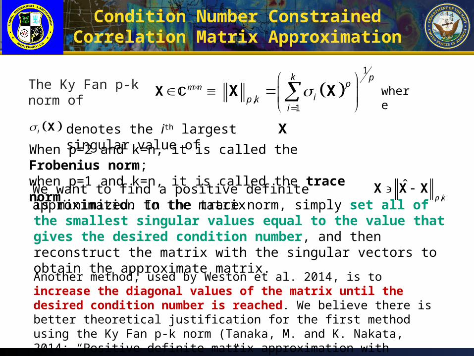
Condition Number Constrained Correlation Matrix Approximation

We want to find a positive definite approximation to the matrix ,

ˆp k

X X Xis minimized. In the trace norm, simply set all of the smallest singular values equal to the value that gives the desired condition number, and then reconstruct the matrix with the singular vectors to obtain the approximate matrix.

Another method, used by Weston et al. 2014, is to increase the diagonal values of the matrix until the desired condition number is reached. We believe there is better theoretical justification for the first method using the Ky Fan p-k norm (Tanaka, M. and K. Nakata, 2014: “Positive definite matrix approximation with condition number constraint”, Optim. Lett. 8, pp 939-947)

1

,1

k pp

ip ki

X XThe Ky Fan p-k norm of m n X where

i X denotes the ith largest singular value of X

When p=2 and k=n, it is called the Frobenius norm;when p=1 and k=n, it is called the trace norm.

12

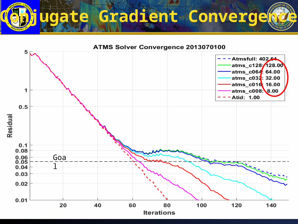
Conjugate Gradient Convergence

Goal

13

• We ran NAVGEM 1.3 at T425L60 resolution with the full suite of operational instruments for two months, from July 1, 2013 through Aug 31, 2013

• The control experiment (atid) used a diagonal R for the ATMS instrument

• The initial ATMS experiment (atms) used the R diagnosed from the Desroziers method applied to three months of innovation statistics

• The second ATMS experiment (atms2) used the R diagnosed from the Desroziers method applied to the first experiment

• Results from these experiments were neutral, but…

Experimental Design

14

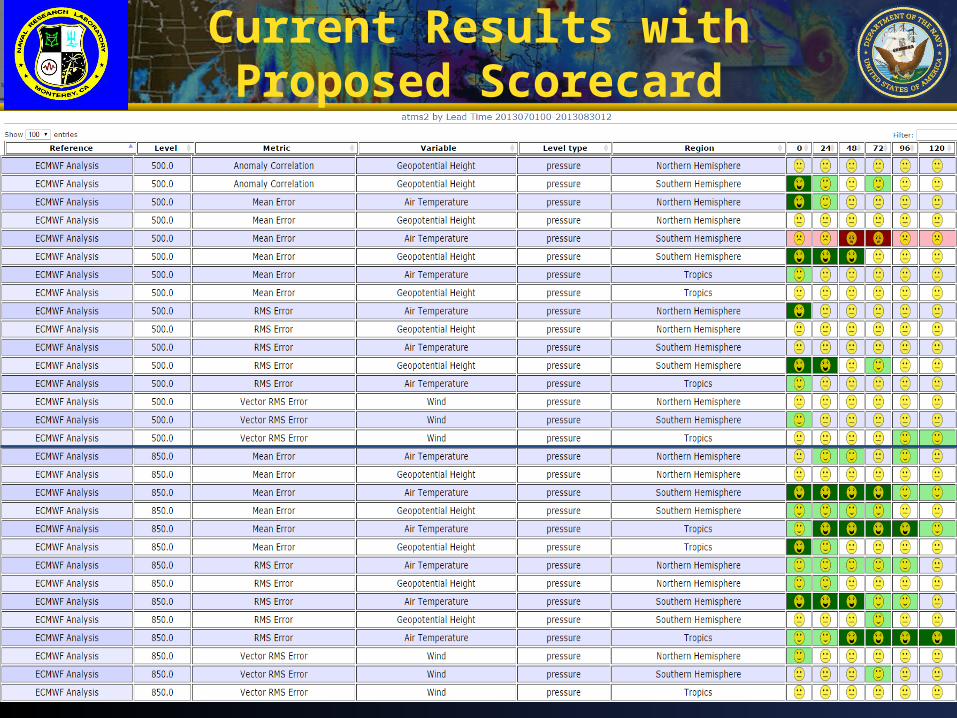
Current Results with Proposed Scorecard

15

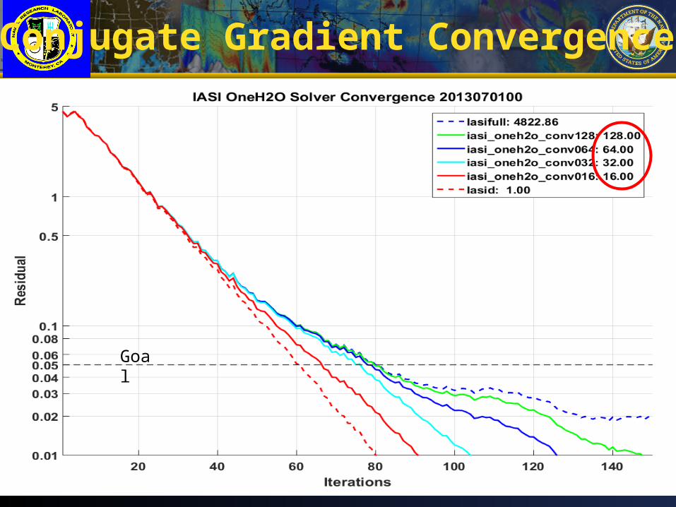
Using the Desroziers Diagnostic for IASI Channel Selection

• Water vapor channels 2889, 2994, 2948, 2951, and 2958 have very high error correlation (>0.98)

• The eigenvectors corresponding to the 4 smallest eigenvalues project only on to these 5 channels

• It makes sense to use the Desroziers diagnostic to do a posteriori channel selection, which has the bonus of improving the condition number of the correlation matrix, and thus solver convergence

16

Conjugate Gradient Convergence

Goal

17

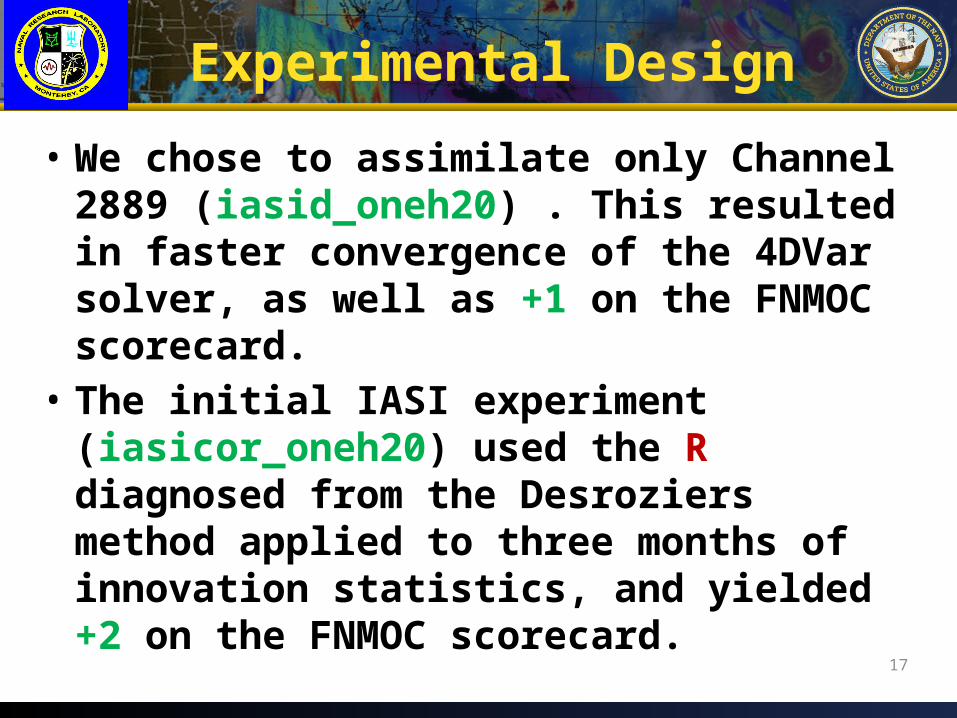
• We chose to assimilate only Channel 2889 (iasid_oneh20) . This resulted in faster convergence of the 4DVar solver, as well as +1 on the FNMOC scorecard.

• The initial IASI experiment (iasicor_oneh20) used the R diagnosed from the Desroziers method applied to three months of innovation statistics, and yielded +2 on the FNMOC scorecard.

Experimental Design

18

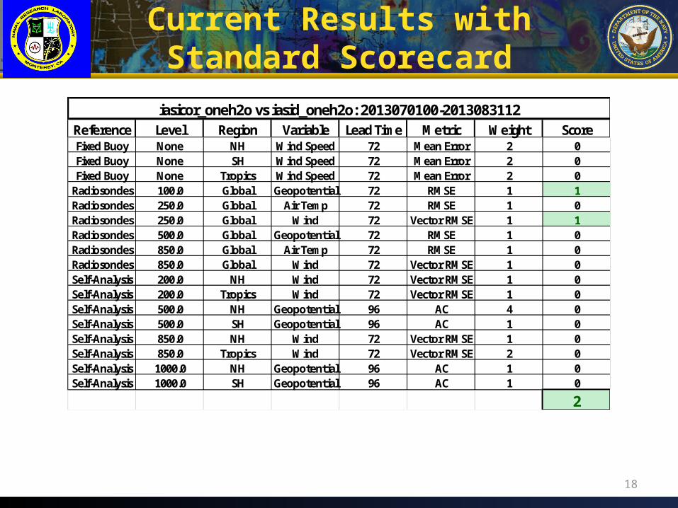
Current Results with Standard Scorecard

Reference Level Region Variable Lead Time Metric Weight ScoreFixed Buoy None NH Wind Speed 72 Mean Error 2 0Fixed Buoy None SH Wind Speed 72 Mean Error 2 0Fixed Buoy None Tropics Wind Speed 72 Mean Error 2 0

Radiosondes 100.0 Global Geopotential 72 RMSE 1 1Radiosondes 250.0 Global Air Temp 72 RMSE 1 0Radiosondes 250.0 Global Wind 72 Vector RMSE 1 1Radiosondes 500.0 Global Geopotential 72 RMSE 1 0Radiosondes 850.0 Global Air Temp 72 RMSE 1 0Radiosondes 850.0 Global Wind 72 Vector RMSE 1 0Self-Analysis 200.0 NH Wind 72 Vector RMSE 1 0Self-Analysis 200.0 Tropics Wind 72 Vector RMSE 1 0Self-Analysis 500.0 NH Geopotential 96 AC 4 0Self-Analysis 500.0 SH Geopotential 96 AC 1 0Self-Analysis 850.0 NH Wind 72 Vector RMSE 1 0Self-Analysis 850.0 Tropics Wind 72 Vector RMSE 2 0Self-Analysis 1000.0 NH Geopotential 96 AC 1 0Self-Analysis 1000.0 SH Geopotential 96 AC 1 0

2

iasicor_oneh2o vs iasid_oneh2o: 2013070100-2013083112

19

• The Desroziers error covariance estimation methods can quantify correlated observation error

• We can make minimal changes to diagnosed error correlations to fit operational time constraints

• The NAVGEM system allows for direct use of a non-diagonal R; implementing vertically correlated error is straightforward

• Correctly accounting for correlated observation error in data assimilation may yield superior forecast results without a large computational cost

Conclusions