Embed Size (px)
Citation preview
Bilateral counterparty risk valuation
for interest-rate products:
impact of volatilities and correlations.
Damiano Brigo∗, Andrea Pallavicini†, Vasileios Papatheodorou‡
First Version: Nov 17, 2009. This Version: February 3, 2010
Abstract
The purpose of this paper is introducing rigorous methods and formulas for bilateralcounterparty risk credit valuation adjustments (CVA’s) on interest-rate portfolios. Indoing so, we summarize the general arbitrage-free valuation framework for counterpartyrisk adjustments in presence of bilateral default risk, as developed more in detail inBrigo and Capponi (2008), including the default of the investor. We illustrate thesymmetry in the valuation and show that the adjustment involves a long position ina put option plus a short position in a call option, both with zero strike and writtenon the residual net present value of the contract at the relevant default times. Weallow for correlation between the default times of the investor and counterparty, andfor correlation of each with the underlying risk factor, namely interest rates. We alsoanalyze the often neglected impact of credit spread volatility. We include Netting inour examples, although other agreements such as Margining and Collateral are left forfuture work.
AMS Classification Codes: 60H10, 60J60, 60J75, 62H20, 91B70JEL Classification Codes: C15, C63, C65, G12, G13
Keywords: Counterparty Risk, Arbitrage-Free Credit Valuation Adjustment, InterestRate Swaps, Interest Rate Derivatives, Credit Valuation Adjustment, Bilateral Risk, CreditSpread Volatility, Default Correlation, Stochastic Intensity, Short Rate Models, Copula Func-tions, Wrong Way Risk.
∗Department of Mathematics, Imperial College, and Fitch Solutions, 101 Finsbury Pavement, EC2A 1RSLondon, UK. E-mail: [email protected]
†Banca Leonardo, Milano, Italy, [email protected]
‡Fitch Solutions, London, UK, E-mail: [email protected]
1
arX
iv:0
911.
3331
v3 [
q-fi
n.PR
] 3
Feb
201
0
D. Brigo, A. Pallavicini and V. Papatheodorou. Bilateral CVA for Interest Rate products 2
Contents
1 Introduction 3
2 Arbitrage-free valuation of bilateral counterparty risk 5
3 Application to Interest Rate Products 83.1 Interest rate model: G2++ . . . . . . . . . . . . . . . . . . . . . . . . . . . . . . . . 83.2 Counterparty and Investor Credit Spread models . . . . . . . . . . . . . . . . . . . . 93.3 Interest-rate / credit-spread correlations . . . . . . . . . . . . . . . . . . . . . . . . . 123.4 Monte Carlo techniques . . . . . . . . . . . . . . . . . . . . . . . . . . . . . . . . . . 12
4 A case study 134.1 Main findings . . . . . . . . . . . . . . . . . . . . . . . . . . . . . . . . . . . . . . . . 154.2 Netted IRS portfolios: right- and wrong-way risk . . . . . . . . . . . . . . . . . . . . 154.3 Netted portfolios and credit spreads . . . . . . . . . . . . . . . . . . . . . . . . . . . 164.4 Netted portfolios and default correlation . . . . . . . . . . . . . . . . . . . . . . . . . 174.5 Netted portfolios and volatility of credit spreads . . . . . . . . . . . . . . . . . . . . 174.6 Netted portfolios and forward rates . . . . . . . . . . . . . . . . . . . . . . . . . . . . 184.7 Exotics . . . . . . . . . . . . . . . . . . . . . . . . . . . . . . . . . . . . . . . . . . . 18
5 Further discussion and conclusions 19
A Interest-rate market data 22
B CDS Terms Structures and Implied Volatilities 22
D. Brigo, A. Pallavicini and V. Papatheodorou. Bilateral CVA for Interest Rate products 3
1 Introduction
This paper deals with pricing of bilateral counterparty risk credit valuation adjustments(CVA’s) on interest-rate portfolios. The structure of the paper is similar to the earlier workof Brigo and Capponi (2008). However, while the focus in Brigo and Capponi (2008) ison Credit Default Swaps (CDS), here it is on interest-rate products, generalizing to thebilateral case the earlier works on unilateral CVA for rates products done by Sorensen andBollier (1994), Brigo and Masetti (2005) and Brigo and Pallavicini (2007). Indeed, previousresearch on accurate arbitrage-free valuation of unilateral CVA with dynamical models oncommodities (Brigo and Bakkar (2009)), on rates (Brigo and Pallavicini (2007)) and on credit(Brigo and Chourdakis (2008)) assumed the party computing the valuation adjustment to bedefault-free. We present here the general arbitrage-free valuation framework for counterpartyrisk adjustments in presence of bilateral default risk, as introduced in Brigo and Capponi(2008), including default of the investor. We illustrate the symmetry in the valuation andshow that the adjustment involves a long position in a put option plus a short position ina call option, both with zero strike and written on the residual net value of the contractat the relevant default times. We allow for correlation between the default times of theinvestor, counterparty and underlying portfolio risk factors. We use arbitrage-free stochasticdynamical models.
We then specialize our analysis to Interest rate payouts as underlying portfolio. Incomparing with the CDS case as underlying, an important point is that most credit modelsin the industry, especially when applied to Collateralized Debt Obligations or k-th to defaultbaskets, model default correlation but ignore credit-spread volatility. Credit spreads aretypically assumed to be deterministic and a copula is postulated on the exponential triggersof the default times to model default correlation. This is the opposite of what used tohappen with counterparty risk for interest-rate underlyings, for example in Sorensen andBollier (1994) or Brigo and Masetti (in Pykhtin (2005)), where correlation was ignored andvolatility was modeled instead. Brigo and Chourdakis (2008) rectify this in the CDS context,but only deal with unilateral and asymmetric counterparty risk. Brigo and Capponi (2008)then generalize this approach for CDS, including credit spread volatility besides defaultcorrelation into the bilateral case.
In interest-rate products, previous literature dealing with both underlying volatility andunderlying/counterparty correlation is in Brigo and Pallavicini (2007), who address bothplain vanilla interest-rate swaps and exotics under unilateral counterparty risk. In thatwork, a stochastic intensity model along the lines of Brigo and Alfonsi (2005) and Brigo andEl-Bachir (2009) is assumed, and this model is correlated with the multi-factor short rateprocess driving the interest-rate dynamics. Netting is also examined in some basic examples.The present paper aims at generalizing this approach to the bilateral case. In such a caseone needs to model the following correlations, or better dependencies:
• Dependence between default of the counterparty and default of the investor;
• Correlation between the underlying (interest rates) and the counterparty credit spread;
• Correlation between the underlying (interest rates) and the investor credit spread;
• Besides default correlation between the counterparty and the investor, we might wishto model also credit spread correlation.
D. Brigo, A. Pallavicini and V. Papatheodorou. Bilateral CVA for Interest Rate products 4
CVA One-sided Bilateral
Modeling Volatility Volatility and Correlation
IR Swaps Brigo Masetti (2005) Brigo Pallavicini (2007) This paperwith Netting
IR Exotics Brigo Pallavicini (2007) This paper
Oil Swaps Brigo Bakkar (2009)
CDS Brigo Chourdakis (2008) Brigo Capponi (2008)
Equity TRS Brigo Tarenghi (2004)Brigo Masetti (2005)
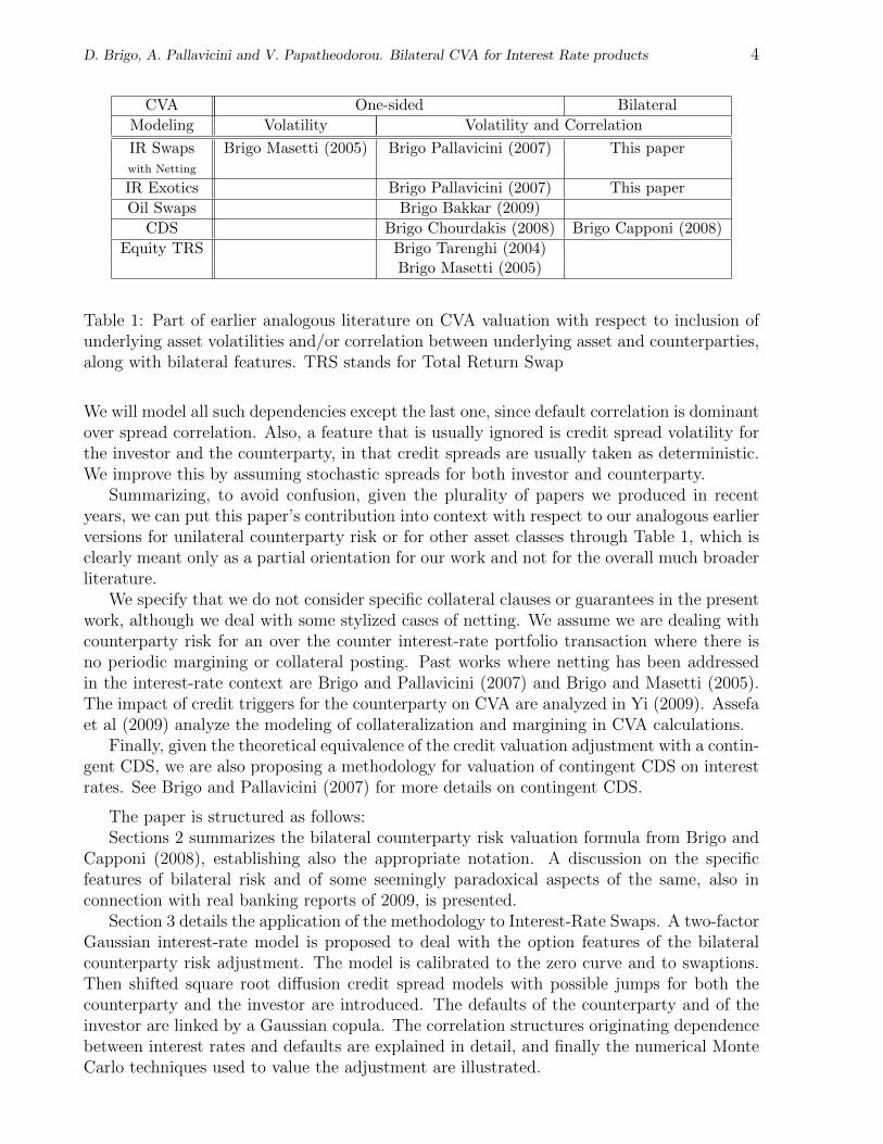
Table 1: Part of earlier analogous literature on CVA valuation with respect to inclusion ofunderlying asset volatilities and/or correlation between underlying asset and counterparties,along with bilateral features. TRS stands for Total Return Swap
We will model all such dependencies except the last one, since default correlation is dominantover spread correlation. Also, a feature that is usually ignored is credit spread volatility forthe investor and the counterparty, in that credit spreads are usually taken as deterministic.We improve this by assuming stochastic spreads for both investor and counterparty.
Summarizing, to avoid confusion, given the plurality of papers we produced in recentyears, we can put this paper’s contribution into context with respect to our analogous earlierversions for unilateral counterparty risk or for other asset classes through Table 1, which isclearly meant only as a partial orientation for our work and not for the overall much broaderliterature.
We specify that we do not consider specific collateral clauses or guarantees in the presentwork, although we deal with some stylized cases of netting. We assume we are dealing withcounterparty risk for an over the counter interest-rate portfolio transaction where there isno periodic margining or collateral posting. Past works where netting has been addressedin the interest-rate context are Brigo and Pallavicini (2007) and Brigo and Masetti (2005).The impact of credit triggers for the counterparty on CVA are analyzed in Yi (2009). Assefaet al (2009) analyze the modeling of collateralization and margining in CVA calculations.
Finally, given the theoretical equivalence of the credit valuation adjustment with a contin-gent CDS, we are also proposing a methodology for valuation of contingent CDS on interestrates. See Brigo and Pallavicini (2007) for more details on contingent CDS.
The paper is structured as follows:Sections 2 summarizes the bilateral counterparty risk valuation formula from Brigo and
Capponi (2008), establishing also the appropriate notation. A discussion on the specificfeatures of bilateral risk and of some seemingly paradoxical aspects of the same, also inconnection with real banking reports of 2009, is presented.
Section 3 details the application of the methodology to Interest-Rate Swaps. A two-factorGaussian interest-rate model is proposed to deal with the option features of the bilateralcounterparty risk adjustment. The model is calibrated to the zero curve and to swaptions.Then shifted square root diffusion credit spread models with possible jumps for both thecounterparty and the investor are introduced. The defaults of the counterparty and of theinvestor are linked by a Gaussian copula. The correlation structures originating dependencebetween interest rates and defaults are explained in detail, and finally the numerical MonteCarlo techniques used to value the adjustment are illustrated.
D. Brigo, A. Pallavicini and V. Papatheodorou. Bilateral CVA for Interest Rate products 5
Section 4 presents a case study based on three possible interest-rate swaps portfolios, someembedding netting clauses. We analyze the impact of credit spread levels and volatilities, ofcorrelations between the underlying interest rates and defaults, and of dependence betweendefault of the counterparty and of the investor. Section 5 concludes the paper.
2 Arbitrage-free valuation of bilateral counterparty risk
The bilateral counterparty risk is mentioned in the Basel II documentation.
Remark 2.1. (Bilateral Counterparty Risk in Basel II, Annex IV, 2/A) “Unlike afirm’s exposure to credit risk through a loan, where the exposure to credit risk is unilateral andonly the lending bank faces the risk of loss, the counterparty credit risk creates a bilateral riskof loss: the market value of the transaction can be positive or negative to either counterpartyto the transaction.”
Basel II is more concerned with Risk Measurement than pricing. For an analysis ofcounterparty risk in the risk-measurement space we refer for example to De Prisco andRosen (2005), who consider modeling of stochastic credit exposures for derivatives portfo-lios. However, also in the valuation space, bilateral features are quite relevant and oftencan be responsible for seemingly paradoxical statements1, as pointed out in Brigo and Cap-poni (2008). For example, Citigroup in its press release on the first quarter revenues of2009 reported a positive mark to market due to its worsened credit quality: “Revenues alsoincluded [...] a net 2.5$ billion positive CVA on derivative positions, excluding monolines,mainly due to the widening of Citi’s CDS spreads”. In this paper we explain precisely howsuch a situation may origin.
We refer to the two names involved in the transaction and subject to default risk as
investor → name “I”
counterparty → name “C”
In general, we will address valuation as seen from the point of view of the investor “I”, sothat cash flows received by “I” will be positive whereas cash flows paid by “I” (and receivedby “C”) will be negative2.
We denote by τI and τC respectively the default times of the investor and counterparty.We place ourselves in a probability space (Ω,G,Gt,Q). The filtration Gt models the flow ofinformation of the whole market, including credit and Q is the risk neutral measure. Thisspace is endowed also with a right-continuous and complete sub-filtration Ft representingall the observable market quantities but the default events, thus Ft ⊆ Gt := Ft ∨ Ht. Here,Ht = σ(τI ≤ u ∨ τC ≤ u : u ≤ t) is the right-continuous filtration generated by thedefault events, either of the investor or of his counterparty.
Let us call T the final maturity of the payoff which we need to evaluate and let us definethe stopping time
τ = minτI , τC (2.1)
1We are grateful to Dan Rosen for first signaling this issue to us during a conference in June 2009
2Here, we follow Brigo and Capponi (2008), although in that paper the investor name “I” is called “0”and the counterparty name “C” is called “2”.
D. Brigo, A. Pallavicini and V. Papatheodorou. Bilateral CVA for Interest Rate products 6
If τ > T , there is neither default of the investor, nor of his counterparty during the life of thecontract and they both can fulfill the agreements of the contract. On the contrary, if τ ≤ Tthen either the investor or his counterparty (or both) default. At τ , the Net Present Value(NPV) of the residual payoff until maturity is computed. We then distinguish two cases:
• τ = τC . If the NPV is negative (respectively positive) for the investor (defaultedcounterparty), it is completely paid (received) by the investor (defaulted counterparty)itself. If the NPV is positive (negative) for the investor (counterparty), only a recoveryfraction RECC of the NPV is exchanged.
• τ = τI . If the NPV is positive (respectively negative) for the defaulted investor (coun-terparty), it is completely received (paid) by the defaulted investor (counterparty)itself. If the NPV is negative (positive) for the defaulted investor (counterparty), onlya recovery fraction RECI of the NPV is exchanged.
Let us define the following (mutually exclusive and exhaustive) events ordering the defaulttimes
A = τI ≤ τC ≤ T E = T ≤ τI ≤ τCB = τI ≤ T ≤ τC F = T ≤ τC ≤ τIC = τC ≤ τI ≤ TD = τC ≤ T ≤ τI (2.2)
Let us call ΠD(t, T ) the discounted payoff of a generic defaultable claim at t and Π(t, T )the discounted payoff for an equivalent claim with a default-free counterparty. We then havethe following Proposition, proven in Brigo and Capponi (2008)
Proposition 2.2. (General bilateral counterparty risk pricing formula) At valua-tion time t, and conditional on the event τ > t, the price of the payoff under bilateralcounterparty risk is
Et[
ΠD(t, T )]
= Et[ Π(t, T ) ]
+Et[
LGDI1A∪BD(t, τI) (−NPV(τI))+ ]
−Et[
LGDC1C∪DD(t, τC) (NPV(τC))+]
(2.3)
where LGDi := 1 − RECi is the Loss Given Default and RECi is the recovery fraction, withi ∈ I, C. It is clear that the value of a defaultable claim is the value of the correspondingdefault-free claim plus a long position in a put option (with zero strike) on the residual NPVgiving nonzero contribution only in scenarios where the investor is the earliest to default(and does so before final maturity) plus a short position in a call option (with zero strike)on the residual NPV giving non-zero contribution in scenarios where the counterparty is theearliest to default (and does so before final maturity).
Definition 2.1. (Bilateral CVA, DVA, CVA) The adjustment is called bilateral counterparty-risk credit-valuation adjustment and it may be either negative or positive depending onwhether the counterparty is more or less likely to default than the investor and on the volatil-ities and correlation. From the investor point of view, we define CVA-BR the adjustment tobe added to the default free price to account for counterparty risk.
D. Brigo, A. Pallavicini and V. Papatheodorou. Bilateral CVA for Interest Rate products 7
When looking at the adjustment from the point of view of the investor “I”, in the righthand side of (2.3) the second term and the third term being subtracted from the secondone are called respectively (unilateral) Debit Valuation Adjustment (DVA) and (unilateral)Credit Valuation Adjustment (CVA), so that the mathematical expression for the bilateraladjustment3 is given by
CVA-BR(t, T ) = DVA(t, T )− CVA(t, T ), (2.4)
DVA(t, T ) = Et[
LGDI1A∪B ·D(t, τI) · (−NPV(τI))+ ]
CVA(t, T ) = Et[
LGDC1C∪D ·D(t, τC) · (NPV(τC))+]
(2.5)
where the right hand side in Equation (2.4) depends on T through the events A,B,C,D andLGDi, with i ∈ I, C, is a shorthand notation to denote the dependence on the loss givendefaults of each name.
Notice that in the paper we assume the recovery fractions (and hence LGD’s) to bedeterministic.
Remark 2.3. (Symmetry vs Asymmetry). With respect to earlier results on counter-party risk valuation, Equation (2.4) has the great advantage of being symmetric. This isto say that if “C” were to compute counterparty risk of her position towards “I”, i.e. theterm to be added to the default free price to include counterparty risk, she would find exactly−CVA-BR(t, T ). However, if each party computed the adjustment to be added by assumingitself to be default-free and considering only the default of the other party, then the adjustmentcalculated by “I” would be
−Et[
LGDC1τC<T ·D(t, τC) · (NPV(τC))+]
whereas the adjustment calculated by “C” would be
−Et[
LGDI1τI<T ·D(t, τI) · (−NPV(τI))+ ]
and they would not be one the opposite of the other. This means that only in the first casethe two parties agree on the value of the counterparty risk adjustment to be added to thedefault-free price.
Remark 2.4. (Change in sign). Earlier results on asymmetric counterparty risk valu-ation, concerned with a default-free investor, would find an adjustment to be added that isalways negative. However, in our symmetric case even if the initial adjustment is negativedue to CVA(t, T ) >DVA(t, T ), i.e.
Et[
LGDC1C∪D ·D(t, τC) · (NPV(τC))+]> Et
[LGDI1A∪B ·D(t, τI) · (−NPV(τI))
+ ]the situation may change in time, to the point that the two terms may cancel or that the
adjustment may change sign as the credit quality of “I” deteriorates and that of “C” improves,so that the inequality changes direction.
Remark 2.5. (Worsening of credit quality and positive mark to market). If theInvestor marks to market her position at a later time using Equation (2.3), we can see thatthe term in LGDI increases, ceteris paribus, if the credit quality of “I” worsens. Indeed, if wefor example increase the credit spreads of the investor, now τI < τC will happen more often,giving more weight to the term in LGDI . This is at the basis of statements like the above oneof Citigroup.
3In Brigo and Capponi (2008) tables report the opposite quantity, −CVA-BR=:BR-CVA=CVA-DVA.
D. Brigo, A. Pallavicini and V. Papatheodorou. Bilateral CVA for Interest Rate products 8
3 Application to Interest Rate Products
In this section we consider a model that is stochastic both in the interest rates (underlyingmarket) and in the default intensity (counterparty). Joint stochasticity is needed to intro-duce correlation. The interest-rate sector is modeled according to a short-rate Gaussianshifted two-factor process (hereafter G2++), while each of the two default-intensity sectorsis modeled according to a square-root process with exponential jumps (hereafter JCIR++).Details for both models can be found, for example, on Brigo and Mercurio (2006). The twomodels are coupled by correlating their Brownian shocks.
3.1 Interest rate model: G2++
For interest rates, we assume that the dynamics of the instantaneous short-rate processunder the risk-neutral measure is given by
r(t) = x(t) + z(t) + ϕ(t;α) , r(0) = r0, (3.1)
where α is a set of parameters and the processes x and z are Ft adapted and satisfy
dx(t) = −ax(t)dt+ σdZ1(t) , x(0) = 0,
dz(t) = −bz(t)dt+ ηdZ2(t) , z(0) = 0,(3.2)
where (Z1, Z2) is a two-dimensional Brownian motion with instantaneous correlation ρ12 asfrom
d〈Z1, Z2〉t = ρ12dt,
where r0, a, b, σ, η are positive constants, and where −1 ≤ ρ12 ≤ 1. These are theparameters entering ϕ, in that α = [r0, a, b, σ, η, ρ12]. The function ϕ(·;α) is deterministicand well defined in the time interval [0, T ∗], with T ∗ a given time horizon, typically 10, 30or 50 (years). In particular, ϕ(0;α) = r0. This function can be set to a value automaticallycalibrating the initial zero coupon curve observed in the market.
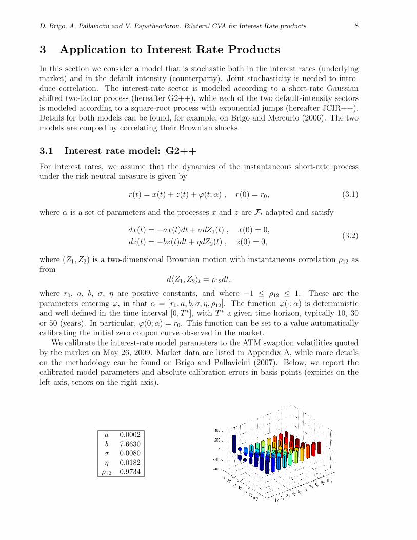
We calibrate the interest-rate model parameters to the ATM swaption volatilities quotedby the market on May 26, 2009. Market data are listed in Appendix A, while more detailson the methodology can be found on Brigo and Pallavicini (2007). Below, we report thecalibrated model parameters and absolute calibration errors in basis points (expiries on theleft axis, tenors on the right axis).
a 0.0002b 7.6630σ 0.0080η 0.0182ρ12 0.9734
D. Brigo, A. Pallavicini and V. Papatheodorou. Bilateral CVA for Interest Rate products 9
The G2++ model links the dependence on tenors of swaption volatilities to the form ofinitial yield curve. Before the crisis period such constraint of the G2++ model seems notso relevant, but the situation changes from spring 2008, when the yield curve steepened inconjunction with a movement in the market volatility surface which could not be reproducedby the model. Yet, versions of the model with time-dependent volatilities can calibrateATM swaption volatilities in a satisfactory way. For instance, if we introduce a time gridt0 = 0, t1, . . . , tm, we can consider the following time-dependent volatilities.
σ(t) := σf(`(t)) , η(t) := ηf(`(t))
where the `(t) := maxt∗ ∈ t0, . . . , tm : t∗ ≤ t function selects the left extremum of eachinterval and
f(t) := 1− e−β1t + β0e−β2t
Notice that in this way we do not alter the analytical tractability of the G2++ model,since all integrals involving model piece-wise-constant parameters can be performed as finitesummations.
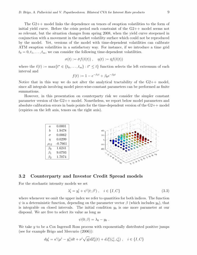
However, in this presentation on counterparty risk we consider the simpler constantparameter version of the G2++ model. Nonetheless, we report below model parameters andabsolute calibration errors in basis points for the time-dependent version of the G2++ model(expiries on the left axis, tenors on the right axis).
a 0.0001b 1.9478σ 0.0062η 0.0299ρ12 -0.7661
β0 1.6241β1 9.0793β2 1.7074
3.2 Counterparty and Investor Credit Spread models
For the stochastic intensity models we set
λit = yit + ψi(t; βi) , i ∈ I, C (3.3)
where whenever we omit the upper index we refer to quantities for both indices. The functionψ is a deterministic function, depending on the parameter vector β (which includes y0), thatis integrable on closed intervals. The initial condition y0 is one more parameter at ourdisposal. We are free to select its value as long as
ψ(0; β) = λ0 − y0 .
We take y to be a Cox Ingersoll Ross process with exponentially distributed positive jumps(see for example Brigo and Mercurio (2006)):
dyit = κi(µi − yit)dt+ νi√yitdZ
i3(t) + dJ it (ζ
i1, ζ
i2) , i ∈ I, C
D. Brigo, A. Pallavicini and V. Papatheodorou. Bilateral CVA for Interest Rate products 10
where the parameter vector is βi := (κi, µi, νi, yi0, ζi1, ζ
i2) and each parameter is a positive
deterministic constant. As usual, Zi3 is a standard Brownian motion process under the risk
neutral measure, while the jump part Jt(ζ1, ζ2) is defined as
J it (ζi1, ζ
i2) :=
M it (ζ
i1)∑
k=1
X ik(ζ
i2) , i ∈ I, C
where M i is a time-homogeneous Poisson process (independent of Z) with intensity ζ i1, theX is being exponentially distributed with positive finite mean ζ i2 independent of M (and Z).The two processes yI and yC are assumed to be independent, so that ZI
3 is independentof ZC
3 and J I is independent of JC (in particular, M I is independent of MC and XI ’s ofXC ’s) . This is assumed to simplify the parametrization of the model and focus on defaultcorrelation rather than spread correlation, but the assumption can be removed if one iswilling to complicate the parametrization of the model.
We define the integrated quantities
Λ(t) :=
∫ t
0
λsds , Y (t) :=
∫ t
0
ysds , Ψ(t, β) :=
∫ t
0
ψ(s, β)ds .
In our Cox process setting the default times are modeled as
τi = (Λi)−1(ξi) , i ∈ I, C
with ξ’s each exponential unit-mean and independent of interest rates. The two ξ are as-sumed to be connected via a bivariate Gaussian copula function with correlation parameterρG. This is a default correlation, and the two default times are connected via default cor-relation, even if their spreads are independent. In fact, in general high default correlationcreates more dependence between the default times than a high correlation in their spreads.
From this setup it follows that when we assume the default intensity λ, and the cumulatedintensity Λ, to be independent of the short rate r and of interest rates in general, also thedefault times τi will be independent of interest-rate related quantities r,D(s, t), .... In thiscase valuation of (running) CDS on reference entities “I” or “C” becomes model independent,leading to
CDSia,b(0, Si) = LGD
[∫ Tb
Ta
P (0, t) dtQ τi ≥ t ]
(3.4)
+Si
−∫ Tb
Ta
P (0, t)(t− Tγ(t)−1) dtQ τi ≥ t +b∑
j=a+1
αjP (0, Tj)Q τi ≥ Tj
where in general Tγ(t) is is the first Tj following t and P (t, T ) = Et[D(t, T ) ] is the zero
coupon bond price at time t for maturity T consistent with the stochastic discount factorsD. This formula is model independent, see for example the credit chapters in Brigo andMercurio (2006) for the details, S is the CDS spread in the premium leg, typically balancingthe default leg at inception. For conversion of these running CDS into upfront ones, followingthe so called Big Bang protocol by ISDA, see for example Beumee, Brigo, Schiemert andStoyle (2009). Since the survival probabilities in the JCIR++ model are given by
Q τ > t model = E0[ exp (−Λ(t)) ] = E0[ exp (−Ψ(t, β)− Y (t)) ] (3.5)
D. Brigo, A. Pallavicini and V. Papatheodorou. Bilateral CVA for Interest Rate products 11
we just need to make sure
E0[ exp (−Ψ(t, β)− Y (t)) ] = Q τ > t CDSmarket
from which
Ψ(t, β) = ln
(E0
[e−Y (t)
]Q τ > t CDSmarket
)= ln
(PJCIR(0, t, y0; β)
Q τ > t CDSmarket
)(3.6)
where we choose the parameters β in order to have a positive function ψ (i.e. an increasingΨ) and PJCIR is the closed form expression for bond prices in the time-homogeneous JCIRmodel with initial condition y0 and parameters β (see for example Brigo and El-Bachir(2009), reported also in Brigo and Mercurio (2006)). Thus, if ψ is selected according to thislast formula, as we will assume from now on, the model is easily and automatically calibratedto the market survival probabilities (possibly stripped from CDS data).
This CDS calibration procedure assumes zero correlation between default and interestrates, so in principle when taking non-zero correlation we cannot adopt it. However, we haveseen in Brigo and Alfonsi (2005) and further in Brigo and Mercurio (2006) that the impactof interest-rate / default correlation is typically small on CDSs, so that we may retain thiscalibration procedure even under non-zero correlation.
Once we have done this and calibrated CDS data through ψ(·, β), we are left with theparameters β, which can be used to calibrate further products. However, this will be in-teresting when single name option data on the credit derivatives market will become moreliquid. Currently the bid-ask spreads for single name CDS options are large and suggest toconsider these quotes with caution, see Brigo (2005). At the moment we content ourselves ofcalibrating only CDS’s for the credit part. To help specifying β without further data we setsome values of the parameters implying possibly reasonable values for the implied volatilityof hypothetical CDS options on the counterparty “C” and investor “I”. Further, we alwaysconsider for the following numerical results that the jump part of the model is switched off.See Brigo and Pallavicini (2007) to size the impact of jumps.
We focus on two different sets of CDS quotes, that we name hereafter Mid and High risksettings. Then, we introduce a different set of model parameters for each CDS setting. Inthe following tables we show them along with the implied volatilities for CDSs starting at tand maturing at T . The implied volatilities are calculated via a Jamshidian’s decompositionas described in Brigo and Alfonsi (2005) or Brigo and Mercurio (2006).
The interest-rate curve is bootstrapped from the market on May 26, 2009 (see Ap-pendix A). Notice that the zero-curve is increasing in time. Further, we always considerthat recovery rates are at 40% level.
We consider two market settings for the credit quality and volatility of “I” and “C”: amid-risk setting and a high risk setting. The mid risk setting parameters are given in Table 2,and the associated CDS term structure and implied volatilities are reported in Appendix B.
y0 κ µ ν0.01 0.80 0.02 0.20
Table 2: Mid risk Credit spread parameters
D. Brigo, A. Pallavicini and V. Papatheodorou. Bilateral CVA for Interest Rate products 12
The High risk market parameters are in Table 3 and the associated CDS term structure andimplied volatilities are reported in Appendix B.
y0 κ µ ν0.03 0.50 0.05 0.50
Table 3: High risk Credit spread parameters
3.3 Interest-rate / credit-spread correlations
We take the short interest-rate factors x and z and the intensity process y to be correlated,by assuming the driving Brownian motions ZI , ZC and Z3 to be instantaneously correlatedaccording to
d〈Zj, Zi3〉t = ρj,idt , j ∈ 1, 2 , i ∈ I, C
Notice that the instantaneous correlation between the resulting short-rate and the inten-sity, i.e. the instantaneous interest-rate / credit-spread correlation is
ρi :=d〈r, λi〉t√
d〈r, r〉t d〈λi, λi〉t=
σρ1i + ηρ2i√σ2 + η2 + 2σηρ12
√1 +
2ζi1ζi2
(νi)2yt
, i ∈ I, C .
This is a state dependent quantity due to presence of jumps. Without jumps, this simplifiesto
ρi =σρ1i + ηρ2i√
σ2 + η2 + 2σηρ12.
In order to reduce the number of free parameters and to model in a more robust way thecorrelation structure of the model, in the following we always consider that
ρ1i = ρ2i , i ∈ I, C .
Further, we prefer to model default correlation by introducing a Gaussian copula on defaulttimes, rather than by correlating the default intensities, so that as explained above we takethe two spread processes yI and yC to be independent.
3.4 Monte Carlo techniques
A Monte Carlo simulation is used to value all the payoffs.The transition density for the G2++ model is known in closed form, while the JCIR++
model, even if we consider the jump part switched off, when correlated with G2++, requiresa discretization scheme for the joint evolution. We find similar convergence results both withthe full truncation scheme introduced by Lord et al. (2006) and with the implied scheme byBrigo and Alfonsi (2005). In the following we adopt the former scheme.
Further, we bucket default times by assuming that the default events can occur only ona time grid Ti : 0 ≤ i ≤ b, with T0 = t and Tb = T , by anticipating each default eventto the last Ti preceding it. In the following calculations we choose a weekly interval and wecheck a-posteriori that the time-grid spacing is small enough to have a stable value for theCVA-BR price.
D. Brigo, A. Pallavicini and V. Papatheodorou. Bilateral CVA for Interest Rate products 13
The calculation of the future time expectation, required by counterparty risk evaluation,is taken by approximating the expectation at the actual (bucketed) default time Ti witha finite series in the interest-rate model underlyings, x and z, on a polynomial basis ψjvalued at the allowed default times within the interval [t, Ti[.
NPV(Ti) := ETi [ Π(Ti, T ) ] =∞∑j=0
αijψj(xt:Ti , zt:Ti) 'N∑j=0
αijψj(xt:Ti , zt:Ti)
Notice that, if the payoff is not time-dependent, the functions ψs need to be valued onlyat Ti. The coefficients αij of the series expansion are calculated by means of a least-squareregression, as usually done to price Bermudan options with the Least Squared Monte Carlomethod.
Thus, the credit valuation adjustment is calculated as follows
CVA-BR(t, T ) ' −LGDC
b−1∑i=0
Et[1τI≥τC1Ti≤τC<Ti+1D(t, Ti) (ETi [ Π(Ti, T ) ])+
]+ LGDI
b−1∑i=0
Et[1τI≤τC1Ti≤τI<Ti+1D(t, Ti) (−ETi [ Π(Ti, T ) ])+
]where the forward expectations are approximated as
ETi [ Π(Ti, T ) ] 'N∑j=0
αijψj(xt:Ti , zt:Ti)
αij = arg minαi0,...,αiN
Et
[(Π(Ti, T )−
N∑j=0
αijψj(xt:Ti , zt:Ti))2 ]
In the following numerical examples we consider non-path-dependent payoffs, and weempirically find stable prices by using a polynomial basis up to the second degree in thefunction parameters, namely
ψ0(x, z) := 1 , ψ1(x, z) := x , ψ2(x, z) := z
ψ3(x, z) := x2 , ψ4(x, z) := z2 , ψ5(x, z) := xz
Notice also that, since the payoff evaluation depends on the projection coefficients which,in turn, depend on the simulated path, we are introducing a correlation between our MonteCarlo samples which, in principle, makes the standard deviation a biased estimator of thestatistical error. However, in our experience the bias introduced by using a single MonteCarlo for both evaluating the αs and the CVA-BR price is negligible.
4 A case study
In the following numerical examples we use as free correlation parameters:
ρC , ρI , ρG .
and we recover the other correlations from them. In particular, we consider the followingcases:
D. Brigo, A. Pallavicini and V. Papatheodorou. Bilateral CVA for Interest Rate products 14
• Varying ρC , keeping fixed ρI = 0.
• Varying both ρC and ρI , keeping them equal, i.e. ρC = ρI .
• For each choice of ρC and ρI , we consider ρG ∈ −80%, 0%, 80%.
We consider payoffs depending on at-the-money forward interest-rate-swap (IRS) payingon the EUR market. These contracts reset a given number of years from trade date andstart accruing two business days later. The IRS’s fixed legs pay annually a 30e/360 strikerate, while the floating legs pay LIBOR twice per year.
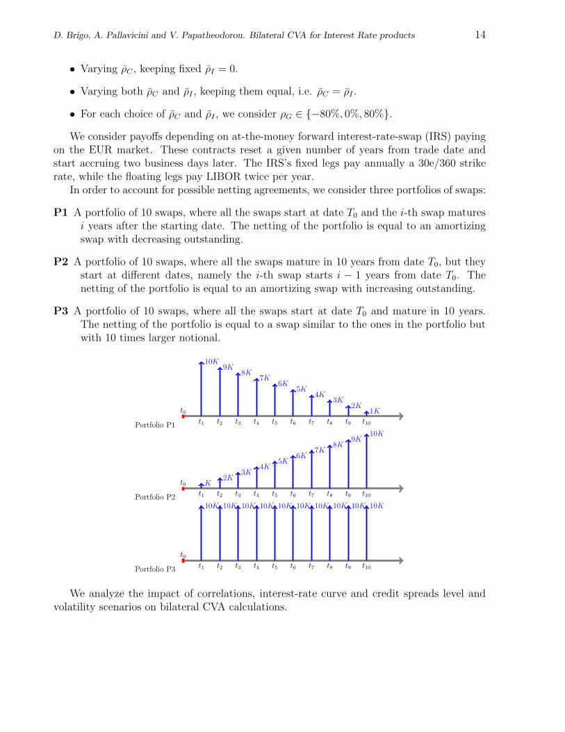
In order to account for possible netting agreements, we consider three portfolios of swaps:
P1 A portfolio of 10 swaps, where all the swaps start at date T0 and the i-th swap maturesi years after the starting date. The netting of the portfolio is equal to an amortizingswap with decreasing outstanding.
P2 A portfolio of 10 swaps, where all the swaps mature in 10 years from date T0, but theystart at different dates, namely the i-th swap starts i − 1 years from date T0. Thenetting of the portfolio is equal to an amortizing swap with increasing outstanding.
P3 A portfolio of 10 swaps, where all the swaps start at date T0 and mature in 10 years.The netting of the portfolio is equal to a swap similar to the ones in the portfolio butwith 10 times larger notional.
Portfolio P1
t0
10K
t1
9K
t2
8K
t3
7K
t4
6K
t5
5K
t6
4K
t7
3K
t8
2K
t9
1K
t10
Portfolio P2
t0 K
t1
2K
t2
3K
t3
4K
t4
5K
t5
6K
t6
7K
t7
8K
t8
9K
t9
10K
t10
Portfolio P3
t0
10K
t1
10K
t2
10K
t3
10K
t4
10K
t5
10K
t6
10K
t7
10K
t8
10K
t9
10K
t10
We analyze the impact of correlations, interest-rate curve and credit spreads level andvolatility scenarios on bilateral CVA calculations.
D. Brigo, A. Pallavicini and V. Papatheodorou. Bilateral CVA for Interest Rate products 15
4.1 Main findings
In general our results confirm, both in the mid- and in the high-risk settings, the bilateralcredit valuation adjustment to be relevant and structured. We in particular notice that theimpact of correlations between investor’s and counterparty’s default risks is relevant. Wealso find a relevant impact of credit spread volatilities for the credit qualities of both names,and of correlation between defaults and interest rates, as was earlier found for unilateralCVA calculations in Brigo and Pallavicini (2007).
Also, in several scenarios the value of CVA-BR may change sign according to the investor’sand the counterparty’s credit risk level and volatilities and depending on the correlation ofthese risks with the interest rates. This change of sign feature is a further convincing reasonof the impact of dynamics on rigorous CVA valuation. The possible change of sign is alsounique of the bilateral case, the unilateral adjustment having always the same sign.
We are going to detail our findings in a number of illustrative examples from our extensiveset of results.
4.2 Netted IRS portfolios: right- and wrong-way risk
Table 4 reports a first panel of results. It is the bilateral credit valuation adjustment forthree different receiver IRS portfolios with ten years maturity, using the high-risk parameterset for the counterparty credit spread and the mid-risk parameter set for the investor creditspread. The two default times are assumed uncorrelated, ρG = 0. This first set considersthe CVA calculation for the three different portfolios for a number of possible behaviours ofwrong-way correlations.
When ρI is kept to zero, we notice the same pattern in ρC we had seen in the unilateralcase in Brigo and Pallavicini (2007). Increasing correlation ρC means that, ceteris paribus,higher interest rates will correspond to high credit spreads, putting the receiver swaptionsembedded in the LGDC term of the adjustment more out of the money. This will cause theLGDC term of the adjustment to diminish in absolute value, so that the final value of theCVA will be larger for high correlation. This is clearly seen in the left panel of Table 4,where the CVA is seen to increase as ρC increases, given that the table columns increase.
When, in the right panel of Table 4, ρI is taken to follow ρC , the behaviour is the samebut more marked. This is reasonable: when ρC is large, also ρI is now large. This meansthat, ceteris paribus, higher interest rates will correspond to high credit spreads, putting thepayer swaptions embedded in the LGDI term of the adjustment more in the money, so thatthis term is larger. This makes the CVA increase further. Not surprisingly, the numbers inthe right panel of Table 4 corresponding to positive correlation (bottom part of the table)are all larger than the corresponding numbers in the left panel.
It is worth finally checking the impact of correlation on the CVA, comparing it withthe typical [1.2, 1.4] interval adjustment factor postulated by Basel II for the credit riskmeasurement correction due to wrong-way risk. Depending on whether we look at the dealfrom the Investor or Counterparty point of view, we find the following ratios between nonzerocorrelation CVA and zero correlation CVA. For example, we find
382/148 ≈ 2.58, 159/31 ≈ 5.13
which are both much larger than 1.4. This means that mimicking the Basel II rules in thevaluation space is not going to work, since the impact of correlations and volatilities is muchmore complex than what can be achieved with a simple multiplier.
D. Brigo, A. Pallavicini and V. Papatheodorou. Bilateral CVA for Interest Rate products 16
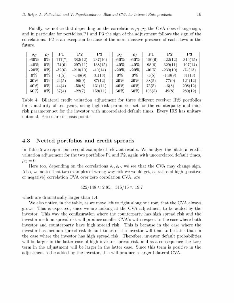
Finally, we notice that depending on the correlations ρI , ρC the CVA does change sign,and in particular for portfolios P1 and P3 the sign of the adjustment follows the sign of thecorrelations. P2 is an exception because of the more massive presence of cash flows in thefuture.
ρC ρI P1 P2 P3
-60% 0% -117(7) -382(12) -237(16)-40% 0% -74(6) -297(11) -138(15)-20% 0% -32(6) -210(10) -40(14)
0% 0% -1(5) -148(9) 31(13)
20% 0% 24(5) -96(9) 87(12)40% 0% 44(4) -50(8) 131(11)60% 0% 57(4) -22(7) 159(11)
ρC ρI P1 P2 P3
-60% -60% -150(6) -422(12) -319(15)-40% -40% -98(6) -329(11) -197(14)-20% -20% -46(5) -230(10) -74(13)
0% 0% -1(5) -148(9) 31(13)
20% 20% 38(5) -77(9) 121(12)40% 40% 75(5) -6(8) 208(12)60% 60% 106(5) 49(8) 280(12)
Table 4: Bilateral credit valuation adjustment for three different receiver IRS portfoliosfor a maturity of ten years, using high-risk parameter set for the counterparty and mid-risk parameter set for the investor with uncorrelated default times. Every IRS has unitarynotional. Prices are in basis points.
4.3 Netted portfolios and credit spreads
In Table 5 we report our second example of relevant results. We analyze the bilateral creditvaluation adjustment for the two portfolios P1 and P2, again with uncorrelated default times,ρG = 0.
Here too, depending on the correlations ρI , ρC , we see that the CVA may change sign.Also, we notice that two examples of wrong-way risk we would get, as ratios of high (positiveor negative) correlation CVA over zero correlation CVA, are
422/148 ≈ 2.85, 315/16 ≈ 19.7
which are dramatically larger than 1.4.We also notice, in the table, as we move left to right along one row, that the CVA always
grows. This is expected, since we are looking at the CVA adjustment to be added by theinvestor. This way the configuration where the counterparty has high spread risk and theinvestor medium spread risk will produce smaller CVA’s with respect to the case where bothinvestor and counterparty have high spread risk. This is because in the case where theinvestor has medium spread risk default times of the investor will tend to be later than inthe case where the investor has high spread risk. Therefore, investor default probabilitieswill be larger in the latter case of high investor spread risk, and as a consequence the LGDI
term in the adjustment will be larger in the latter case. Since this term is positive in theadjustment to be added by the investor, this will produce a larger bilateral CVA.
D. Brigo, A. Pallavicini and V. Papatheodorou. Bilateral CVA for Interest Rate products 17
ρC ρI H/M H/H M/H
-60% -60% -150(6) -76(7) 47(5)-40% -40% -98(6) -12(6) 97(5)-20% -20% -46(5) 48(6) 135(5)
0% 0% -1(5) 110(6) 187(6)
20% 20% 38(5) 173(6) 241(6)40% 40% 75(5) 239(7) 297(6)60% 60% 106(5) 304(7) 361(7)
ρC ρI H/M H/H M/H
-60% -60% -422(12) -284(12) -40(9)-40% -40% -329(11) -179(12) 36(9)-20% -20% -230(10) -77(10) 102(9)
0% 0% -148(10) 16(10) 179(9)
20% 20% -77(9) 112(10) 262(10)40% 40% -6(9) 218(10) 351(10)60% 60% 49(9) 315(11) 450(11)
Table 5: Bilateral credit valuation adjustment, by changing the parameter set, for a decreas-ing (P1, left panel) and an increasing (P2, right panel) IRS portfolio for a maturity of tenyears, with uncorrelated default times. Every IRS has unitary notional. Prices are in basispoints.
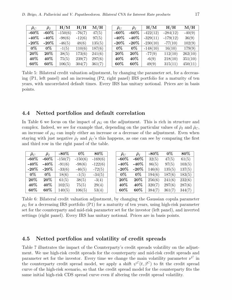
4.4 Netted portfolios and default correlation
In Table 6 we focus on the impact of ρG on the adjustment. This is rich in structure andcomplex. Indeed, we see for example that, depending on the particular values of ρI and ρC ,an increase of ρG can imply either an increase or a decrease of the adjustment. Even whenstaying with just negative ρI and ρC ’s this happens, as one can see by comparing the firstand third row in the right panel of the table.
ρC ρI -80% 0% 80%
-60% -60% -150(7) -150(6) -169(6)-40% -40% -91(6) -98(6) -122(6)-20% -20% -33(6) -46(5) -72(5)
0% 0% 18(6) -1(5) -34(5)
20% 20% 61(5) 38(5) -3(4)40% 40% 102(5) 75(5) 29(4)60% 60% 140(5) 106(5) 53(4)
ρC ρI -80% 0% 80%
-60% -60% 32(5) 47(5) 61(5)-40% -40% 86(5) 97(5) 103(5)-20% -20% 146(6) 135(5) 137(5)
0% 0% 194(6) 187(6) 183(5)
20% 20% 256(6) 241(6) 232(6)40% 40% 320(7) 297(6) 287(6)60% 60% 384(7) 361(7) 344(7)
Table 6: Bilateral credit valuation adjustment, by changing the Gaussian copula parameterρG for a decreasing IRS portfolio (P1) for a maturity of ten years, using high-risk parameterset for the counterparty and mid-risk parameter set for the investor (left panel), and invertedsettings (right panel). Every IRS has unitary notional. Prices are in basis points.
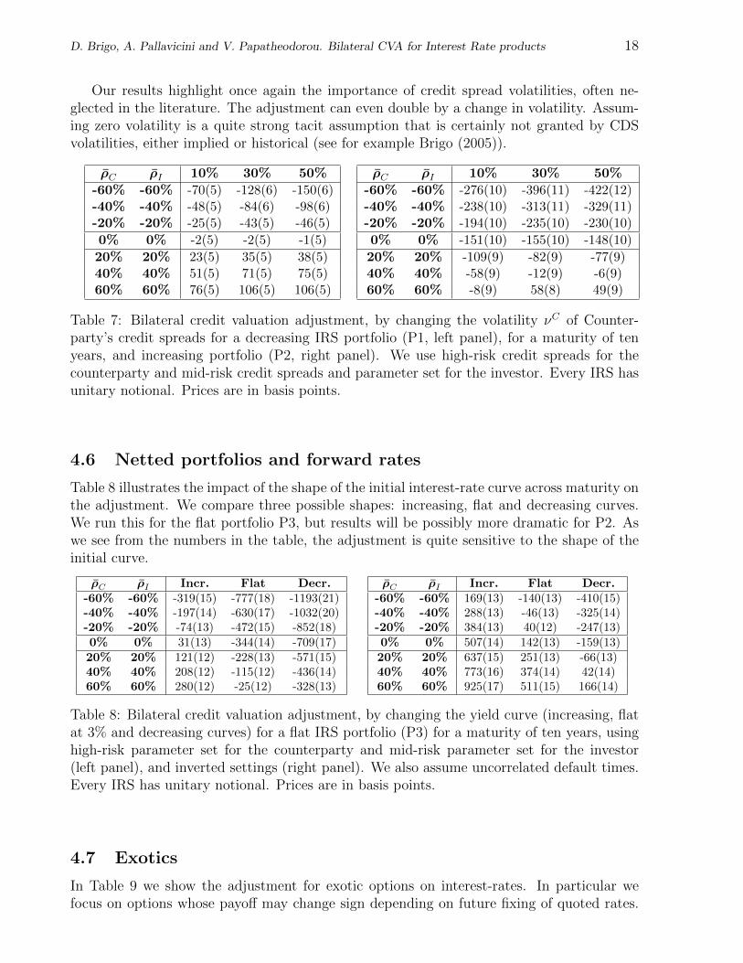
4.5 Netted portfolios and volatility of credit spreads
Table 7 illustrates the impact of the Counterparty’s credit spreads volatility on the adjust-ment. We use high-risk credit spreads for the counterparty and mid-risk credit spreads andparameter set for the investor. Every time we change the main volatility parameter νC inthe counterparty credit spread model, we apply a shift ψC(t, βC) to fit the credit spreadcurve of the high-risk scenario, so that the credit spread model for the counterparty fits thesame initial high-risk CDS spread curve even if altering the credit spread volatility.
D. Brigo, A. Pallavicini and V. Papatheodorou. Bilateral CVA for Interest Rate products 18
Our results highlight once again the importance of credit spread volatilities, often ne-glected in the literature. The adjustment can even double by a change in volatility. Assum-ing zero volatility is a quite strong tacit assumption that is certainly not granted by CDSvolatilities, either implied or historical (see for example Brigo (2005)).
ρC ρI 10% 30% 50%
-60% -60% -70(5) -128(6) -150(6)-40% -40% -48(5) -84(6) -98(6)-20% -20% -25(5) -43(5) -46(5)
0% 0% -2(5) -2(5) -1(5)
20% 20% 23(5) 35(5) 38(5)40% 40% 51(5) 71(5) 75(5)60% 60% 76(5) 106(5) 106(5)
ρC ρI 10% 30% 50%
-60% -60% -276(10) -396(11) -422(12)-40% -40% -238(10) -313(11) -329(11)-20% -20% -194(10) -235(10) -230(10)
0% 0% -151(10) -155(10) -148(10)
20% 20% -109(9) -82(9) -77(9)40% 40% -58(9) -12(9) -6(9)60% 60% -8(9) 58(8) 49(9)
Table 7: Bilateral credit valuation adjustment, by changing the volatility νC of Counter-party’s credit spreads for a decreasing IRS portfolio (P1, left panel), for a maturity of tenyears, and increasing portfolio (P2, right panel). We use high-risk credit spreads for thecounterparty and mid-risk credit spreads and parameter set for the investor. Every IRS hasunitary notional. Prices are in basis points.
4.6 Netted portfolios and forward rates
Table 8 illustrates the impact of the shape of the initial interest-rate curve across maturity onthe adjustment. We compare three possible shapes: increasing, flat and decreasing curves.We run this for the flat portfolio P3, but results will be possibly more dramatic for P2. Aswe see from the numbers in the table, the adjustment is quite sensitive to the shape of theinitial curve.
ρC ρI Incr. Flat Decr.-60% -60% -319(15) -777(18) -1193(21)-40% -40% -197(14) -630(17) -1032(20)-20% -20% -74(13) -472(15) -852(18)0% 0% 31(13) -344(14) -709(17)20% 20% 121(12) -228(13) -571(15)40% 40% 208(12) -115(12) -436(14)60% 60% 280(12) -25(12) -328(13)
ρC ρI Incr. Flat Decr.-60% -60% 169(13) -140(13) -410(15)-40% -40% 288(13) -46(13) -325(14)-20% -20% 384(13) 40(12) -247(13)0% 0% 507(14) 142(13) -159(13)20% 20% 637(15) 251(13) -66(13)40% 40% 773(16) 374(14) 42(14)60% 60% 925(17) 511(15) 166(14)
Table 8: Bilateral credit valuation adjustment, by changing the yield curve (increasing, flatat 3% and decreasing curves) for a flat IRS portfolio (P3) for a maturity of ten years, usinghigh-risk parameter set for the counterparty and mid-risk parameter set for the investor(left panel), and inverted settings (right panel). We also assume uncorrelated default times.Every IRS has unitary notional. Prices are in basis points.
4.7 Exotics
In Table 9 we show the adjustment for exotic options on interest-rates. In particular wefocus on options whose payoff may change sign depending on future fixing of quoted rates.
D. Brigo, A. Pallavicini and V. Papatheodorou. Bilateral CVA for Interest Rate products 19
The calculation of one-sided CVA for exotic interest-rate options is covered in Brigo andPallavicini (2007). Here we address the bilateral case.
For instance, we consider IRS portfolio P3, and we add an auto-callable feature triggeredby the Libor rate, namely we exit form the IRS contract when on a fix-leg payment date thefixing of the Libor rate is greater then a strike level A. We can appreciate that also for thisproduct the correlations have quite an impact on the value of the adjustment.
ρC ρI -99% 0% 99%
-70% -70% -71 -64 -550% 0% -47 -43 -3470% 70% -28 -26 -20
Table 9: Bilateral credit valuation adjustment, by changing the Gaussian copula parameterρG, for an auto-callable IRS portfolio (P3) for a maturity of ten years, using high-risk pa-rameter set for the counterparty and mid-risk parameter set for the investor. The contracthas unitary notional. Prices are in basis points. Intrinsic price is 608, with an auto-callablestrike level of A = 3%.
5 Further discussion and conclusions
In general our results confirm the bilateral credit valuation adjustment to be quite sensitiveto finely tuned dynamics parameters such as volatilities and correlations, similarly to whatwas found in Brigo and Capponi (2008) for the CDS market. The impact of the parametersis both relevant and structured.
We in particular noticed the impact of correlations between investor’s and counterparty’sdefault risks, of credit spread volatilities for the credit qualities of both names, of creditspread levels and of correlations between defaults and interest rates. Variations in theseparameters can produce an excursion in the adjustment of several multiples or even have theadjustment changing in sign.
In particular, there seems to be no single multiple that can provide the adjustmentfor high correlations starting from the adjustment with zero correlations. Hence the needto include such correlations in the modeling apparatus in a rigorous way. We proposed apossible modeling choice for addressing this, with a two-factor Gaussian model (G2++) forinterest rates and shifted square root processes with possible jumps (JCIR++) for the creditspreads of investor and counterparty. Defaults of the two names are linked by a Gaussiancopula function.
We detailed our findings in a number of illustrative examples from an extensive set ofresults.
D. Brigo, A. Pallavicini and V. Papatheodorou. Bilateral CVA for Interest Rate products 20
References
[1] Assefa, S., Bielecki, T., Crepey, S., and Jeanblanc, M. (2009). CVA computation forcounterparty risk assesment in credit portfolio. Preprint.
[2] Beumee, J., Brigo, D., Schiemert, D., and Stoyle, G. (2009). Charting a Course Throughthe CDS Big Bang. Fitch Solutions research report.
[3] Bielecki, T., Jeanblanc, M., and Rutkowski M. (2008). Hedging of Credit Default Swap-tions in a Hazard Process Model. Available at www.defaultrisk.com.
[4] Blanchet-Scalliet, C., and Patras, F. (2008). Counterparty Risk Valuation for CDS.Available at www.defaultrisk.com.
[5] Brigo, D. (2005). Market Models for CDS Options and Callable Floaters. Risk, Januaryissue.
[6] Brigo, D. (2008). Counterparty Risk valuation with Stochastic Dynamical Models: Im-pact of Volatilities and Correlations. Talk at fifth World Business Strategies Fixed In-come Conference, Budapest, 26 September.
[7] Brigo, D., and Capponi, A. (2008). Bilateral counterparty risk valuation with stochasticdynamical models and application to Credit Default Swaps. Available at ssrn.com orat arxiv.org.
[8] Brigo, D., and Alfonsi A. (2005). Credit Default Swap Calibration and DerivativesPricing with the SSRD Stochastic Intensity Model, Finance and Stochastic, 9, 29.
[9] Brigo, D., and Bakkar I. (2009). Accurate counterparty risk valuation for energy-commodities swaps. Energy Risk, March issue.
[10] Brigo, D., and El-Bachir, N. (2009). An exact formula for default swaptions’ pricing inthe SSRJD stochastic intensity model. Mathematical Finance in press.
[11] Brigo, D., and Chourdakis, K. (2008). Counterparty Risk for Credit Default Swaps:Impact of spread volatility and default correlation. International Journal of Theoreticaland Applied Finance in press.
[12] Brigo, D., and Masetti, M. (2005). Risk Neutral Pricing of Counterparty Risk. In Coun-terparty Credit Risk Modelling: Risk Management, Pricing and Regulation, Risk Books,Pykhtin, M. editor, London.
[13] Brigo, D., and Mercurio, F. (2006). Interest Rate Models: Theory and Practice – withSmile, Inflation and Credit. Second Edition, Springer Verlag, 2006.
[14] Brigo, D., and Pallavicini A. (2007). Counterparty Risk under Correlation betweenDefault and Interest Rates. In Numerical Methods for Finance, Chapman Hall, Miller,J., Edelman, D., and Appleby, J. editors.
[15] Brigo D., Tarenghi M. (2004), Credit Default Swap Calibration and Equity Swap Val-uation under Counterparty risk with a Tractable Structural Model, Working Paper(Available at www.ssrn.com and www.defaultrisk.com).
D. Brigo, A. Pallavicini and V. Papatheodorou. Bilateral CVA for Interest Rate products 21
[16] Collin-Dufresne P., Goldstein R., and Hugonnier J. (2004). A general formula for pricingdefaultable securities. Econometrica, 72, 1377.
[17] Cox, J., Ingersoll, J., and Ross, S. (1985). A theory of the term structure of interestrates. Econometrica, 53, 385.
[18] Chourdakis, K. (2005). Option pricing using the fractional FFT. Journal of Computa-tional Finance, 8, 1.
[19] Crepey, S., Jeanblanc, M., and B. Zargari (2009). CDS with Counterparty Risk in aMarkov Chain Copula Model with Joint Defaults. Available at www.defaultrisk.com.
[20] De Prisco, B., and Rosen, D. (2005). Modelling Stochastic Counterparty Credit Expo-sures for Derivatives Portfolios. In Counterparty Credit Risk Modelling: Risk Manage-ment, Pricing and Regulation, Risk Books, Pykhtin, M. editor, London.
[21] Duffie, D., and Lando, D. (2001). Term structure of credit spreads with incompleteaccounting information. Econometrica, 63, 633.
[22] Hille, C.T., J. Ring and H. Shimanmoto (2005). Modelling Counterparty Credit Expo-sure for Credit Default Swaps. In Counterparty Credit Risk Modelling: Risk Manage-ment, Pricing and Regulation, Risk Books, Pykhtin, M. editor, London.
[23] Hull, J., and White, A. (2000). Valuing credit default swaps: Modelling default corre-lations. Working paper, University of Toronto, 2000.
[24] Leung, S.Y., and Kwok, Y. K. (2005). Credit Default Swap Valuation with CounterpartyRisk. The Kyoto Economic Review, 74, 25.
[25] Lipton, A., and Sepp, A. (2009). Credit value adjustment for credit default swaps viathe structural default model. Journal of Credit Risk, 5, 123.
[26] Picoult, E. (2005). Calculating and Hedging Exposure, Credit Value Adjustment andEconomic Capital for Counterparty Credit Risk In Counterparty Credit Risk Modelling:Risk Management, Pricing and Regulation, Risk Books, Pykhtin, M. editor, London.
[27] Pykhtin, M. (2005). Editor of Counterparty Credit Risk Modelling: Risk Management,Pricing and Regulation, Risk Books, London.
[28] Sorensen, E. H. and Thierry F. Bollier (1994). Pricing Swap Default Risk, FinancialAnalysts Journal, 50, 23.
[29] Yi, C. (2009). Dangerous Knowledge: Credit Value Adjustment with Credit Triggers.Bank of Montreal research paper.
[30] Walker, M. (2005). Credit Default Swaps with Counterparty Risk: A Calibrated MarkovModel. Available at www.physics.utoronto.ca/$\sim$qocmp/CDScptyNew.pdf.
D. Brigo, A. Pallavicini and V. Papatheodorou. Bilateral CVA for Interest Rate products 22
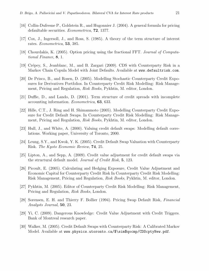
A Interest-rate market data
We report the yield curve term structure and swaption volatilities used to calibrate theinterest-rate and credit-spread dynamics in Sections 3.1 and 3.2.
Date Rate Date Rate Date Rate
27-May-09 1.15% 28-Dec-09 1.49% 29-May-17 3.40%28-May-09 1.02% 28-Jan-10 1.53% 28-May-18 3.54%29-May-09 0.98% 26-Feb-10 1.56% 28-May-19 3.66%04-Jun-09 0.93% 29-Mar-10 1.59% 28-May-21 3.87%11-Jun-09 0.92% 28-Apr-10 1.61% 28-May-24 4.09%18-Jun-09 0.91% 28-May-10 1.63% 28-May-29 4.19%29-Jun-09 0.91% 30-May-11 1.72% 29-May-34 4.07%28-Jul-09 1.05% 28-May-12 2.13% 30-May-39 3.92%28-Aug-09 1.26% 28-May-13 2.48%28-Sep-09 1.34% 28-May-14 2.78%28-Oct-09 1.41% 28-May-15 3.02%30-Nov-09 1.46% 30-May-16 3.23%
Table 10: EUR zero-coupon continuously-compounded spot rates (ACT/360) observed onMay, 26 2009.
t ↓ / b→ 1y 2y 3y 4y 5y 6y 7y 8y 9y 10y
1y 42.8% 34.3% 31.0% 28.8% 27.7% 26.9% 26.5% 26.3% 26.2% 26.2%2y 28.7% 25.6% 24.1% 23.1% 22.4% 22.3% 22.2% 22.3% 22.4% 22.4%3y 23.5% 21.1% 20.4% 20.0% 19.7% 19.7% 19.7% 19.8% 19.9% 20.1%4y 19.9% 18.5% 18.2% 18.1% 18.0% 18.1% 18.1% 18.2% 18.2% 18.4%5y 17.6% 16.8% 16.9% 16.9% 17.0% 16.9% 17.0% 17.0% 17.0% 17.1%7y 15.4% 15.3% 15.3% 15.3% 15.3% 15.3% 15.3% 15.4% 15.5% 15.6%10y 14.2% 14.2% 14.2% 14.3% 14.4% 14.5% 14.6% 14.7% 14.8% 15.0%
Table 11: Market at-the-money swaption volatilities observed on May, 26 2009. Each columncontains volatilities of swaptions of a given tenor b for different expiries t.
B CDS Terms Structures and Implied Volatilities
We report the CDS term structures and implied volatilities associated with the model pa-rameter used for the credit-spread dynamics in Section 3.2.
T 1y 2y 3y 4y 5y 6y 7y 8y 9y 10yCDS Spread 92 104 112 117 120 122 124 125 126 127
Table 12: Mid risk initial CDS term structure
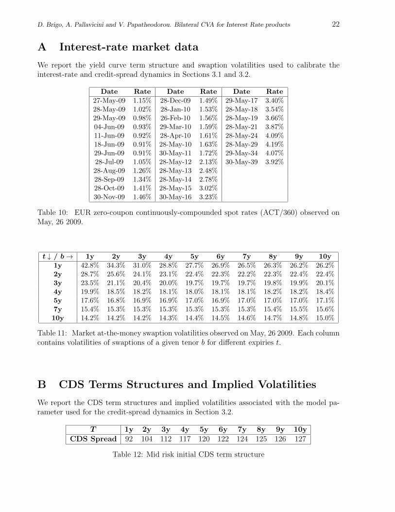
D. Brigo, A. Pallavicini and V. Papatheodorou. Bilateral CVA for Interest Rate products 23
t ↓ / T → 2y 3y 4y 5y 6y 7y 8y 9y 10y
1y 52% 36% 27% 21% 17% 15% 13% 12% 11%2y 39% 28% 21% 17% 14% 12% 11% 10%3y 33% 24% 18% 15% 12% 11% 9%4y 29% 21% 16% 13% 11% 9%5y 26% 19% 15% 12% 10%6y 24% 17% 13% 11%7y 23% 16% 12%8y 21% 15%9y 19%
Table 13: Mid risk CDS implied volatility associated to the parameters in Table 2. Eachcolumn contains volatilities of CDS options of a given maturity T for different expiries t.
T 1y 2y 3y 4y 5y 6y 7y 8y 9y 10yCDS Spread 234 244 248 250 252 252 254 253 254 254
Table 14: High risk initial CDS term structure
t ↓ / T → 2y 3y 4y 5y 6y 7y 8y 9y 10y
1y 96% 69% 53% 43% 36% 31% 28% 26% 24%2y 71% 52% 40% 32% 27% 24% 21% 19%3y 59% 43% 33% 26% 22% 20% 18%4y 51% 37% 28% 23% 20% 17%5y 45% 33% 26% 21% 18%6y 40% 30% 24% 19%7y 40% 29% 22%8y 36% 26%9y 34%
Table 15: High risk CDS implied volatility associated to the parameters in Table 3. Eachcolumn contains volatilities of CDS options of a given maturity T for different expiries t.


![FundingValuationAdjustment ... · The works Brigo et al. [2011c] and Brigo et al. [2011b] look at CVA and DVA gap risk under several collateralization strategies, with or without](https://img.pdfslide.us/doc/110x75/5be837f309d3f2d3638cfb81/fundingvaluationadjustment-the-works-brigo-et-al-2011c-and-brigo-et-al.jpg)