Embed Size (px)
Citation preview
NBER WORKING PAPER SERIES
BIG DATA IN FINANCE AND THE GROWTH OF LARGE FIRMS
Juliane BegenauMaryam FarboodiLaura Veldkamp
Working Paper 24550http://www.nber.org/papers/w24550
NATIONAL BUREAU OF ECONOMIC RESEARCH1050 Massachusetts Avenue
Cambridge, MA 02138April 2018
This paper was prepared for the Carnegie-Rochester-NYU conference. We thank the conference committee for their support of this work. We also thank Nic Kozeniauskas for his valuable assistance with the data and Adam Lee for his outstanding research assistance. The views expressed herein are those of the authors and do not necessarily reflect the views of the National Bureau of Economic Research.
At least one co-author has disclosed a financial relationship of potential relevance for this research. Further information is available online at http://www.nber.org/papers/w24550.ack
NBER working papers are circulated for discussion and comment purposes. They have not been peer-reviewed or been subject to the review by the NBER Board of Directors that accompanies official NBER publications.
© 2018 by Juliane Begenau, Maryam Farboodi, and Laura Veldkamp. All rights reserved. Short sections of text, not to exceed two paragraphs, may be quoted without explicit permission provided that full credit, including © notice, is given to the source.

Big Data in Finance and the Growth of Large FirmsJuliane Begenau, Maryam Farboodi, and Laura VeldkampNBER Working Paper No. 24550April 2018JEL No. E2,G1,D8
ABSTRACT
One of the most important trends in modern macroeconomics is the shift from small firms to large firms. At the same time, financial markets have been transformed by advances in information technology. We explore the hypothesis that the use of big data in financial markets has lowered the cost of capital for large firms, relative to small ones, enabling large firms to grow larger. Large firms, with more economic activity and a longer firm history offer more data to process. As faster processors crunch ever more data – macro announcements, earnings statements, competitors' performance metrics, export demand, etc. – large firms become more valuable targets for this data analysis. Once processed, that data can better forecast firm value, reduce the risk of equity investment, and thus reduce the firm's cost of capital. As big data technology improves, large firms attract a more than proportional share of the data processing, enabling large firms to invest cheaply and grow larger.
Juliane BegenauGraduate School of BusinessStanford University655 Knight WayStanford, CA 94305and [email protected]
Maryam Farboodi26 Prospect AveBendheim Center for FinancePrinceton UniversityPrinceton, NJ [email protected]
Laura VeldkampStern School of BusinessNew York University44 W Fourth Street,Suite 7-77New York, NY 10012and [email protected]
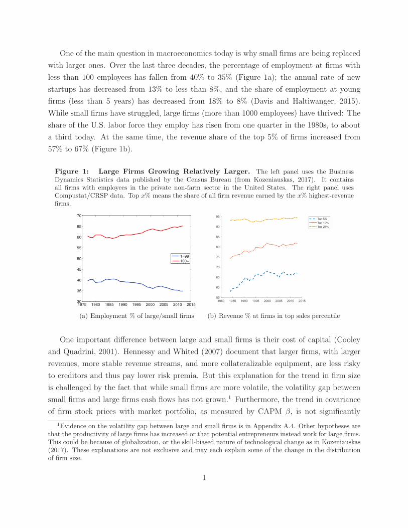
One of the main question in macroeconomics today is why small firms are being replaced
with larger ones. Over the last three decades, the percentage of employment at firms with
less than 100 employees has fallen from 40% to 35% (Figure 1a); the annual rate of new
startups has decreased from 13% to less than 8%, and the share of employment at young
firms (less than 5 years) has decreased from 18% to 8% (Davis and Haltiwanger, 2015).
While small firms have struggled, large firms (more than 1000 employees) have thrived: The
share of the U.S. labor force they employ has risen from one quarter in the 1980s, to about
a third today. At the same time, the revenue share of the top 5% of firms increased from
57% to 67% (Figure 1b).
Figure 1: Large Firms Growing Relatively Larger. The left panel uses the BusinessDynamics Statistics data published by the Census Bureau (from Kozeniauskas, 2017). It containsall firms with employees in the private non-farm sector in the United States. The right panel usesCompustat/CRSP data. Top x% means the share of all firm revenue earned by the x% highest-revenuefirms.
1975 1980 1985 1990 1995 2000 2005 2010 201530
35
40
45
50
55
60
65
70
1−99
100+
(a) Employment % of large/small firms
1980 1985 1990 1995 2000 2005 2010 201555
60
65
70
75
80
85
90
95Top 5%
Top 10%
Top 25%
(b) Revenue % at firms in top sales percentile
One important difference between large and small firms is their cost of capital (Cooley
and Quadrini, 2001). Hennessy and Whited (2007) document that larger firms, with larger
revenues, more stable revenue streams, and more collateralizable equipment, are less risky
to creditors and thus pay lower risk premia. But this explanation for the trend in firm size
is challenged by the fact that while small firms are more volatile, the volatility gap between
small firms and large firms cash flows has not grown.1 Furthermore, the trend in covariance
of firm stock prices with market portfolio, as measured by CAPM β, is not significantly
1Evidence on the volatility gap between large and small firms is in Appendix A.4. Other hypotheses arethat the productivity of large firms has increased or that potential entrepreneurs instead work for large firms.This could be because of globalization, or the skill-biased nature of technological change as in Kozeniauskas(2017). These explanations are not exclusive and may each explain some of the change in the distributionof firm size.
1

different across firms of different sizes.
If neither volatility nor covariance with market risk has diverged, how could risk premia
and thus the cost of capital diverge? What introduces a wedge between unconditional vari-
ance or covariance and risk is information. Even if the payoff variance is constant, better
information can make payoffs more predictable and therefore less uncertain. Given this new
data, the conditional payoff variance and covariance fall. More predictable payoffs lower
risk and lower the cost of capital. The strong link between information and the cost of
capital is supported empirically by Fang and Peress (2009), who find that media coverage
lowers the expected return on stocks that are more widely covered. This line of reasoning
points to an information-related trend in financial markets that has affected the abundance
of information about large firms relative to small firms. What is this big trend in financial
information? It is the big data revolution.
Our goal is to explore the hypothesis that the use of big data in financial markets has
lowered the cost of capital for large firms relative to small ones, enabling large firms to grow
larger. In modern financial markets, information technology is pervasive and transformative.
Faster and faster processors crunch ever more data: macro announcements, earnings state-
ments, competitors’ performance metrics, export market demand, anything and everything
that might possibly forecast future returns. This data informs the expectations of modern
investors and reduces their uncertainty about investment outcomes. More data processing
lowers uncertainty, which reduces risk premia and the cost of capital, making investments
more attractive.
To explore and quantify these trends in modern computing and finance, we use a noisy
rational expectations model where investors choose how to allocate digital bits of information
processing power among various firm risks, and then use that processed information to solve
a portfolio problem. The key insight of the model is that the investment-stimulating effect
of big data is not spread evenly across firms. Small firms benefit less. In our model, small
firms are equivalent to young firms, and large firms to old firms. This is consistent with
the data, where age and size are positively correlated. In the model, larger firms are more
valuable targets for data analysis because more economic activity and a longer firm history
generates more data to process. In contrast, all the computing power in the world cannot
inform an investor about a small firm that has a short history with few disclosures. As big
data technology improves, large firms attract a more than proportional share of the data
processing. Because data resolves risk, the gap in the risk premia between large and small
firms widens. Such an asset pricing pattern enables large firms to invest cheaply and grow
2

larger.
The data side of the model builds on theory designed to explain human information
processing (Kacperczyk et al., 2016), and embeds it into a standard model of corporate
finance and investment decisions (Gomes, 2001). In this type of model, deviations from
Modigliani-Miller imply that the cost of capital matters for firms’ investment decisions. In
our model, the only friction affecting the cost of capital works through the information
channel. The big data allocation model can be reduced to a sequence of required returns for
each firm that depends on the data-processing ability and firm size. These required returns
can then be plugged into a standard firm investment model. To keep things as simple as
possible, we study the big-data effect on firms’ investment decisions based on a simulated
sample of firms – two, in our case – in the spirit of Hennessy and Whited (2007).
The key link between data and real investment is the price of newly-issued equity. Assets
in this economy are priced according to a conditional CAPM, where the conditional variance
and covariance are those of a fictitious investor who has the average precision of all investors’
information. The more data the average investor processes about an asset’s payoff, the
lower is the asset’s conditional variance and covariance with the market. A researcher who
estimated a traditional, unconditional CAPM would attribute these changes to a relative
decline in the excess returns (alphas) on small firms. Thus, the widening spread in data
analysis implies that the alphas of small firm stocks have fallen relative to larger firms. These
asset pricing moments are new testable model predictions that can be used to evaluate and
refine big data investment theories.
Our model serves both to showcase a new mechanism and as a framework for measure-
ment. Obviously, there are other forces that affect firm size. We do not build in many other
contributing factors. Instead, we opt to keep our model stylized, which allows a transparent
analysis of the new role that big data plays. Our question is simply how much of the change
in the size distribution is this big data mechanism capable of explaining? We use data in
combination with the model to understand how changes in the amount of data processed
over time affect asset prices of large and small public firms, and how these trends reconcile
with the size trends in the full sample of firms. An additional challenge is measuring the
amount of data. Using information metrics from computer science, we can map the growth
of CPU speeds to signal precisions in our model. By calibrating the model parameters to
match the size of risk premia, price informativeness, initial firm size and volatility, we can de-
termine whether the effect of big data on firms’ cost of capital is trivial or if it is a potentially
substantial contributor to the missing small firm puzzle.
3
Contribution to the existing literature Our model combines features from a few dis-
parate literatures. The topic of changes in the firm size distribution has been taken up
in many recent papers, including Davis and Haltiwanger (2015), Kozeniauskas (2017), and
Akcigit and Kerr (2017). In addition, a number of papers analyze how size affects the cost
of capital, e.g. Cooley and Quadrini (2001), Hennessy and Whited (2007), and Begenau
and Salomao (2018). We explore a very different force that affects firm size and quantify its
effect.
Another strand of literature explores the feedback between information in financial mar-
kets and investment: Maksimovic et al. (1999) models the relationship between a firm’s cap-
ital structure and its information acquisition prior to capital budgeting decisions. Bernhardt
et al. (1995) studies the effect of different levels of insider trading on investment. Ozdenoren
and Yuan (2008) studies a setting where asset prices influence fundamentals through coor-
dinated buying and thus self-fulfilling beliefs. Furthermore, there are papers that focus on
long run data or information trends in finance: Asriyan and Vanasco (2014), Biais et al.
(2015) and Glode et al. (2012) model growth in fundamental analysis or an increase in its
speed. The idea of long-run growth in information processing is supported by the rise in
price informativeness documented by Bai et al. (2016).
Over time, it has gotten easier and easier to process large amounts of data. As in Farboodi
et al. (2017), this growing amount of data reduces the uncertainty of investing in a given
firm. But the new idea that this paper adds to the existing work on data and information
frictions, is this: Intensive data crunching works well to reduce uncertainty about large firms
with long histories and abundant data. For smaller firms, who tend also to be younger firms,
data may be scarce. Big data technology only reduces uncertainty if abundant data exists to
process. Thus as big data technology has improved, the investment uncertainty gap between
large and small firms has widened, their costs of financing have diverged, and big firms have
grown ever bigger.
1 Model
We develop a model whose purpose is to understand how the growth in big data technologies
in finance affects firm size and gauge the size of that effect. The model builds on the
information choice model in Kacperczyk et al. (2016) and Kacperczyk et al. (2015).
4

1.1 Setup
This is a repeated, static model. Each period has the following sequence of events. First,
firms choose entry and firm size. Second, investors choose how to allocate their data process-
ing across different assets. Third, all investors choose their portfolios of risky and riskless
assets. At the end of the period, asset payoffs and utility are realized. The next period, new
investors arrive and the same sequence repeats. What changes between periods is that firms
accumulate capital and the ability to process big data grows over time.
Firm Decisions We assume that firms are equity financed. Each firm i has a profitable
1-period investment opportunity and wants to issue new equity to raise capital for that
investment. For every share of capital invested, the firm can produce a stochastic payoff
fi,t. Thus total firm output depends on the scale of the investment, which is the number of
shares xi,t, and the output per share fi,t:
yi,t = xi,tfi,t. (1)
The owner of the firm chooses how many shares xi,t to issue. The owner’s objective is
to maximize the revenue raised from the sale of the firm, net of the setup or investment cost
φ(xi,t, xi,t−1) = φ01(|∆xi,t|>0) + φ1|∆xi,t|+ φ2(∆xi,t)2, (2)
where ∆xi,t = xi,t− xi,t−1, 1|∆xi,t|>0 is an indicator function taking the value of one if |∆xi,t|
is strictly positive and φ0, φ1, φ2 > 0. This cost function represents the idea that issuing new
equity (or buying equity back) has a fixed cost φ0 and a marginal cost that is increasing in
the number of new shares issued. Each share sells at price pi,t, which is determined by the
investment market equilibrium. The owner’s objective is thus
Evi,t = E[xi,tpi,t − φ(xi,t, xi,t−1)|It−1], (3)
which is the expected net revenue from the sale of firm i.
The firm makes its choice conditional on the same prior information that all the investors
have and understanding the equilibrium behavior of investors in the asset market. But the
firm does not condition on pi,t. In other words, it does not take prices as given. Rather, the
firm chooses xi,t, taking into account its impact on the equilibrium price.
5

Assets The model features 1 riskless and n risky assets. The price of the riskless asset is
normalized to 1 and it pays off rt at the end of period t. Risky assets i ∈ {1, ..., n} have
random payoffs fi,t ∼ N(µ,Σ) , where Σ is a diagonal “prior” variance matrix.2 We define
the n× 1 vector ft = [f1,t, f2,t, . . . , fn,t]′ .
Each asset has a stochastic supply given by xi,t + xi,t, where noise xi,t is normally
distributed, with mean zero, variance σx, and no correlation with other noises: xt ∼
N (0, σxI). As in any (standard) noisy rational expectations equilibrium model, the supply
is random to prevent the price from fully revealing the information of informed investors.
Portfolio Choice Problem There is a continuum of measure one of atomless investors.
Each investor is endowed with begining-of-period wealth, Wt.3 They have mean-variance
preferences over end-of-period wealth, with a risk-aversion coefficient, ρ. Let Ej,t and Vj,t
denote investor j’s period t expectations and variances conditioned on all interim information,
which includes prices and signals. Thus, investor j chooses how many shares of each asset
to hold, qj,t to maximize period t interim expected utility, Uj,t:
Uj,t = ρEj,t[Wj,t]−ρ2
2Vj,t[Wj,t], (4)
subject to the budget constraint:
Wj,t = rtWt + q′j,t(ft − ptrt), (5)
where qj,t and pt are n× 1 vectors of prices and quantities of each asset held by investor j.
Prices Equilibrium prices are determined by market clearing:
∫ 1
0
qj,tdj = xt + xt, (6)
where the left-hand side of the equation is the vector of aggregate demand and the right-hand
side is the vector of aggregate supply of the assets.
2We can allow assets to be correlated. To solve a correlated asset problem simply requires constructingportfolios of assets (risk factors) that are independent from each other, choosing how much to invest and learnabout these risk factors, and then projecting the solution back on the original asset space. See Kacperczyket al. (2016) for such a solution.
3Since there are no wealth effects in the preferences, the assumption of identical initial wealth is withoutloss of generality.
6
Information sets, updating, and data allocation At the start of each period, each
investor j chooses the amount of data that she will receive at the interim stage, before she
invests. A piece of data is a signal about the risky asset payoff. A time-t signal, indexed by
l, about asset i is ηl,i,t = fi,t + el,i,t, where the data error el,i,t is independent across pieces
of data l, across investors, across assets i and over time. Signal noise is normally distributed
and unbiased: el,i,t ∼ N(0, σe/δ). By Bayes’ law, choosing to observe M signals, each with
signal noise variance σe/δ, is equivalent to observing one signal with signal noise variance
σe/(Mδ), or equivalently, precision Mδ/σe. The discreteness in signals complicates the
analysis, without adding insight. But if we have a constraint that allows an investor to
process M/δ pieces of data, each with precision δ/σe, and then we take the limit δ → 0, we
get a quasi-continuous choice problem. The choice of how many pieces of data to process
about each asset becomes equivalent to choosing Ki,j,t, the precision of investor j’s signal
about asset i in period t. Investor j’s vector of data-equivalent signals about each asset
is ηj,t = ft + εj,t, where the vector of signal noise is distributed as εj,t ∼ N (0,Ση,j,t).The
variance matrix Ση,j,t is diagonal with the ith diagonal element K−1i,j,t. Investors combine
signal realizations with priors and information extracted from asset prices to update their
beliefs using Bayes’ law.
Signal precision choices {Ki,j,t} maximize start-of-period expected utility, Uj,t, of the
fund’s terminal wealth Wj,t. Thus the objective is
max{Ki,j,t}ni=1E[Uj,t|I
+t−1] (7)
where It = {I+t−1, ηjt, pt} and I+
t−1 = {It−1, xt−1, ft−1} (8)
subject to the the budget constraint (5) and three constraints in the information choices.4
The first constraint is the information capacity constraint. It states that the sum of the
signal precisions must not exceed the information capacity:
n∑
i=1
Ki,j,t ≤ Kt for each j, t. (9)
In Bayesian updating with normal variables, observing one signal with precision Ki,j,t or
two signals, each with precision Ki,j,t/2, is equivalent. Therefore, one interpretation of
the capacity constraint is that it allows the manager to observe N signal draws, each with
4See Veldkamp (2011) for a discussion of the use of expected mean-variance utility in information choiceproblems.
7
precision Ki,j,t/N , for large N . The investment manager then chooses how many of those
N signals will be about each shock.5
The second constraint is the data availability constraint. It states that the amount of
data processed about the future earnings of firm i cannot exceed the total data generated
by the firm. Since data is a by-product of economic activity, data availability depends on
the economic activity of the firm in the previous period. In other words, data availability in
time t is a function of firm size in t− 1.
Ki,j,t ≤ K(xi,t−1) for all i, j, t. (10)
This limit on data availability is a new feature of the model. It is also what links firm size
to the expected cost of capital.6 We assume that the data availability constraint takes a
simple, exponential form: K(xi,t−1) = α exp (βxi,t−1).
The third constraint is the no-forgetting constraint, which ensures that the chosen preci-
sions are non-negative:
Ki,j,t ≥ 0 for all i, j, t. (11)
It prevents the manager from erasing any prior information to make room to gather new
information about another asset.
1.2 Equilibrium
To solve the model, we begin by working through the mechanics of Bayesian updating. There
are three types of information that are aggregated in posterior beliefs: prior beliefs, price
information, and (private) signals. We conjecture and later verify that a transformation
of prices pt generates an unbiased signal about the risky payoffs, ηp,t = ft + ǫp,t, where
ǫp,t ∼ N(0,Σp,t), for some diagonal variance matrix Σp,t. Then, by Bayes’ law, the posterior
beliefs about ft are normally distributed: ft ∼ N(Ej,t[ft], Σj,t), where the posterior mean
5The results are not sensitive to the exact nature of the information capacity constraint. We could insteadspecify a cost function of data processing c(Ki,j,t). The problem we solve is the dual of this cost functionapproach. For any cost function, there exists a constraint value Kt such that the cost function problem andthe constrained problem yield identical solutions.
6As our model does not distinguish between size and age, the data availabality constraint can also bethought of linking firm age to the expected cost of capital.
8

and precision are given by:
Ej,t[ft] = Σj,t(Σ−1µ+ Σ−1
η,j,tηj,t + Σ−1p,tηp,t), (12)
Σ−1j,t = Σ−1 + Σ−1
p,t + Σ−1η,j,t. (13)
Next, we solve the model in four steps.
Step 1: Solve for the optimal portfolios, given information sets and issuance.
Substituting the budget constraint (5) into the objective function (4) and taking the
first-order condition with respect to qj,t reveals that optimal holdings are increasing in the
investor’s risk tolerance, precision of beliefs, and expected return:
q∗j,t =1
ρΣ−1
j,t (Ej,t[ft]− ptrt). (14)
Step 2: Clear the asset market.
Substitute each agent j’s optimal portfolio (14) into the market-clearing condition (6).
Collecting terms and simplifying reveals that equilibrium asset prices are linear in payoff risk
shocks and in supply shocks:
Lemma 1. pt =1rt(At +Bt(ft − µ) + Ctxt) .
A detailed derivation of coefficients At, Bt, and Ct, expected utility, and the proofs of
this lemma and all further propositions are in the Appendix.
In this model, agents learn from prices because prices are informative about the asset
payoffs ft. Next, we deduce what information is implied by Lemma 1. Price information
is the signal about ft contained in prices. The transformation of the price vector pt that
yields an unbiased signal about ft is µ + ηp,t ≡ B−1t (ptrt − At). Note that applying the
formula for ηp,t to Lemma 1 reveals that ηp,t = ft + εp,t, where the signal noise in prices
is εp,t = B−1t Ctxt. Since we assumed that xt ∼ N(0, σxI), the price noise is distributed
εp,t ∼ N(0,Σp,t), where Σp,t ≡ σxB−1t CtC
′tB
−1′
t . Substituting in the coefficients Bt and Ct
from the proof of Lemma 1 shows that public signal precision Σ−1p,t is a diagonal matrix with
ith diagonal element σ−1p,i,t =
K2
i,t
ρ2σx, where Ki,t ≡
∫
Ki,j,tdj is the average capacity allocated
to asset i.
This market-clearing asset price reveals the firm’s cost of capital. We define the cost of
capital as follows.
9

Definition 1. The cost of capital for firm i is the difference between the (unconditional)
expected payout per share the firm will make to investors, minus the (unconditional) expected
price per share that the investor will pay to the firm: Et[fi,t]− Et[pi,t].
Because xt is a mean-zero random variable and the payoff ft has mean µ, the uncondi-
tional expected price is Et[pi,t] = Ai,t/r. Therefore, the expected cost of capital for firm i is
µ− Ai,t/r.
Step 3: Compute ex-ante expected utility.
Substitute optimal risky asset holdings from equation (14) into the first-period objective
function (7) to get: Uj,t = ρrtWt+12Et[(Ej,t[ft]−ptrt)
′Σ−1j,t (Ej,t[ft]−ptrt)]. Note that the ex-
pected excess return (Ej,t[ft]−ptrt) depends on signals and prices, both of which are unknown
at the start of the period. Because asset prices are linear functions of normally distributed
shocks, Ej,t[ft]−ptrt, is normally distributed as well. Thus, (Ej,t[ft]−ptrt)Σ−1j,t (Ej,t[ft]−ptrt)
is a non-central χ2-distributed variable. Computing its mean yields:
Uj,t = ρrtWt +1
2tr(Σ−1
j,t Vj,t[Ej,t[ft]− ptrt]) +1
2Ej,t[Ej,t[ft]− ptrt]
′Σ−1j,t Ej,t[Ej,t[ft]− ptrt].
(15)
Step 4: Solve for information choices.
Note that in expected utility (15), the choice variables Ki,j,t enter only through the
posterior variance Σj,t and through Vj,t[Ej,t[ft] − ptrt] = Vj,t[f − ptrt] − Σj,t. Since there
is a continuum of investors, and since Vj,t[f − ptrt] and Ej,t[Ej,t[ft] − ptrt] depend only on
parameters and on aggregate information choices, each investor takes them as given.
Since Σ−1j,t and Vj,t[Ej,t[ft]− ptrt] are both diagonal matrices and Ej,t[Ej,t[ft]− ptrt] is a
vector, the last two terms of (15) are weighted sums of the diagonal elements of Σ−1j,t . Thus,
(15) can be rewritten as Uj,t = rtWt +∑
i λi,tΣ−1j,t (i, i) − n/2, for positive coefficients λi,t.
Since rtWt is a constant (in each period t) and Σ−1j,t (i, i) = Σ−1(i, i) +Σ−1
p,t (i, i) +Ki,j,t, the
information choice problem is:
maxK1,j,t,...,Kn,j,t≥0
n∑
i=1
λi,tKi,j,t + constant, (16)
s.t.n
∑
i=1
Ki,j,t ≤ Kt, (17)
Ki,j,t ≤ α exp (βxi,t−1) ∀i , ∀j, (18)
where λi,t = σi,t[1 + (ρ2σx + Ki,t)σi,t] + ρ2x2i,tσ
2i,t, (19)
10

where λi,t is the marginal value of information σ−1i,t =
∫
Σ−1j,t (i, i)dj is the average precision
of posterior beliefs about firm i. The latter’s inverse, average variance σi,t, is decreasing in
Ki,t. Equation (19) is derived in the Appendix.
This is not a concave objective, so a first-order approach will not find an optimal data
choice. To maximize a weighted sum (16) subject to an unweighted sum (17), the investor op-
timally assigns all available data, as per (18), to the asset(s) with the highest weight. If there
is a unique i∗t = argmaxi λi,t, then the solution is to set Ki∗t ,j,t= min(Kt, α exp (βxi,t−1)).
In many cases, after all data processing capacity is allocated, there will be multiple assets
with identical λi,t weights. That is because λi,t is decreasing in the average investor’s signal
precision. When there exist asset factor risks i, l s.t. λi,t = λl,t, then investors are indifferent
about which assets’ data to process. The next result shows that this indifference is not a
knife-edge case. It arises whenever the aggregate amount of data processing capacity is
sufficiently high.
Lemma 2. If xi,t is sufficiently large ∀i and∑
i
∑
j Ki,j,t ≥ K, then there exist risks l and
l′ such that λl,t = λl′,t.
This is the big data analog to Grossman and Stiglitz (1980)’s strategic substitutability in
information acquisition. The more other investors know about an asset, the more informative
prices are and the less valuable it is for other investors to process data about the same asset.
If one asset has the highest marginal utility for signal precision, but capacity is high, then
many investors will learn about that asset, causing its marginal utility to fall and equalize
with the next most valuable asset data. With more capacity, the highest two λi,t’s will be
driven down until they equate with the next λi,t, and so forth. This type of equilibrium is
called a “waterfilling” solution (see, Cover and Thomas (1991)). The equilibrium uniquely
pins down which assets are being learned about in equilibrium, and how much is learned
about them, but not which investor learns about which asset.
Step 5: Solve for firm equity issuance. How a firm chooses xt depends on how issuance
affects the asset price. Supply xt enters the asset price in only one place in the equilibrium
pricing formula, through At. From Appendix equation (33), we see that
At = µ− ρΣtxt. (20)
xt has a direct effect on the second term. But also an indirect effect through information
choices that show up in Σt.
11
The firm’s choice of xt satisfies its first order condition:
E[pt|It−1]− xt
(
ρΣt − ρxt
∂Σt
∂xt
)
− φ′1(xt, xt−1) = 0. (21)
The first term is the benefit of more issuance. When a firm issues an additional share,
it gets expected revenue E[pt|It−1] for that share. The second term tells us that issuance
has a positive and negative effect on the share price. The negative effect on the price is that
more issuance raises the equity premium ( ρΣt term). The positive price effect is that more
issuance makes data on the firm more valuable to investors. When investors process more
data on the firm, it lowers their investment risk, and on average, raises the price they are
willing to pay ( ∂Σt/∂xt term). This is the part of the firm investment decision that the rise
of big data will affect.
The third term, the capital adjustment cost ( φ′1(xt, xt−1)), reveals why firms grow in size
over time. Firms have to pay to adjust relative to their intial size. Since firms’ starting size
is small they want to grow, but rapid growth is costly. So, they grow gradually. Each time
a firm starts larger, choosing a higher xt becomes less costly because the size of the change,
and thus the adjustment cost is smaller.
Note that in our static model adjustment costs perform a slightly different function
compared to a dynamic model. In the static model, the main role of adjustment costs is to
link the initial and final size together, in order to generate cross-sectional differences in the
marginal value of information. Larger firms can afford to choose a larger final scale. The
larger the final scale, the higher the marginal value of information.
2 Parameter Choice
In order to quantify the potential effect of big data on firm size, we need to perform a quan-
titative exercise. What changes exogenously at each date is the total information capacity
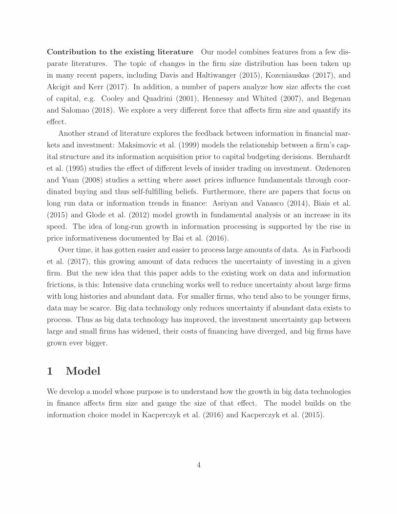
Kt. We normalize Kt = 1 in 1980 and then grow Kt continuously, at the rate of 36.8% per
year: Kt+1 = Kte0.368. This rate of growth corresponds to the average rate of growth of CPU
speed, as illustrated in Figure 2. We simulate the model in this fashion from 1980-2030. As
Kt increases over time, constraint (9) becomes looser, allowing for a larger overall sum of
signal precisions.
We also need to choose values for the model parameters. For µ, σ, σx, r, we use the same
values as in the numerical example in the supplementary appendix to Kacperczyk et al.
12
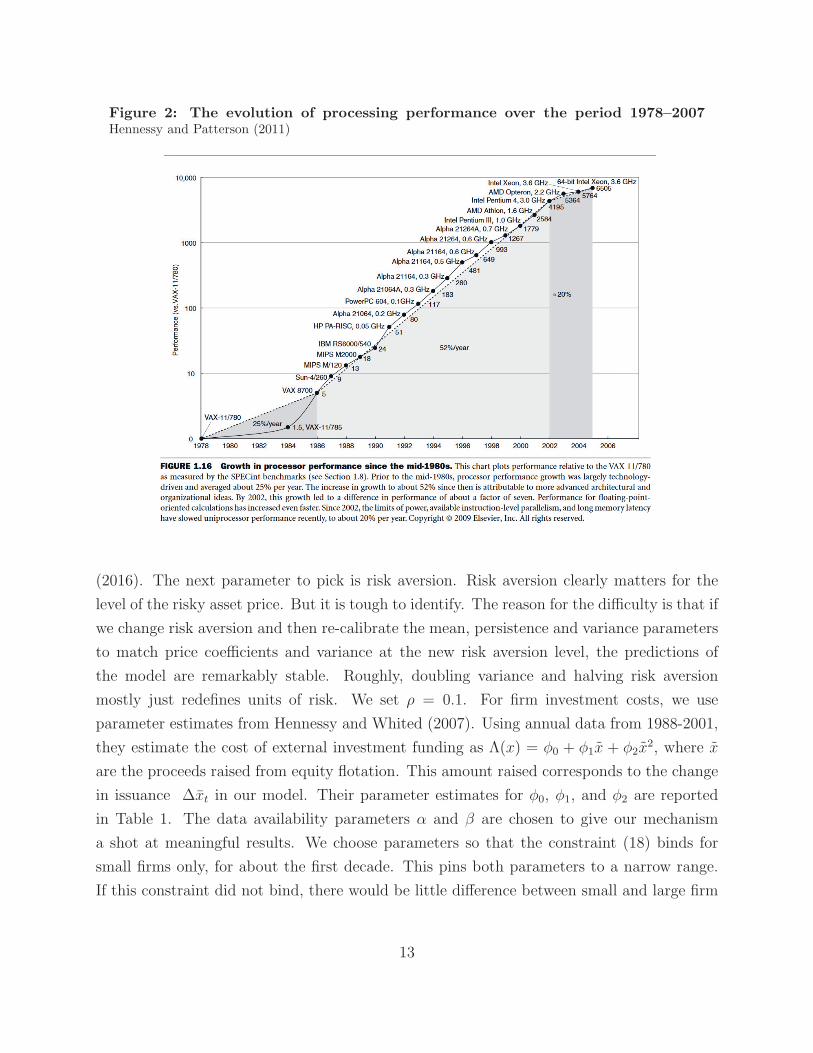
Figure 2: The evolution of processing performance over the period 1978–2007Hennessy and Patterson (2011)
(2016). The next parameter to pick is risk aversion. Risk aversion clearly matters for the
level of the risky asset price. But it is tough to identify. The reason for the difficulty is that if
we change risk aversion and then re-calibrate the mean, persistence and variance parameters
to match price coefficients and variance at the new risk aversion level, the predictions of
the model are remarkably stable. Roughly, doubling variance and halving risk aversion
mostly just redefines units of risk. We set ρ = 0.1. For firm investment costs, we use
parameter estimates from Hennessy and Whited (2007). Using annual data from 1988-2001,
they estimate the cost of external investment funding as Λ(x) = φ0 + φ1x + φ2x2, where x
are the proceeds raised from equity flotation. This amount raised corresponds to the change
in issuance ∆xt in our model. Their parameter estimates for φ0, φ1, and φ2 are reported
in Table 1. The data availability parameters α and β are chosen to give our mechanism
a shot at meaningful results. We choose parameters so that the constraint (18) binds for
small firms only, for about the first decade. This pins both parameters to a narrow range.
If this constraint did not bind, there would be little difference between small and large firm
13

outcomes. If the availability constraint was binding for all firms, then there would be no
effect of big data growth because there would be insufficient data to process with the growing
processing power.
Table 1: Parameters
µ σ σx rt φ0 φ1 φ2 ρ α β15 0.55 0.5 1.01 0.598 0.091 0.0004 0.1 0.249 0.0002
3 Quantitative Results
Our main results use the simulated model to understand how the growth of big data affects
the evolution of large and small firms and how large that effect might be. We start by
exploring how the rise in big data availability changes how data is allocated. Then, we
explore how changes in data the investors observe affect the firm’s cost of capital. Finally,
we turn to the question of how much the change in data and the cost of capital affect the
evolution of firms that start out small and firms that start out large.
In presenting our results, we try to balance realism with simplicity, which illuminates the
mechanism. If we put in a large number of firms, it is, of course, more realistic. But this
would also make it harder to see what the trade-offs are. Instead, we characterize the firm
distribution with one representative large firm and one representative small firm. The two
firms are identical, except that the large firm starts off with a larger size x0 = 10, 000. The
small firm starts off with x0 = 2, 000. Starting in 1980, we simulate our economy with the
parameters listed in Table 1 with one period per year until 2030.
3.1 Data Allocation Choices
The reason that data choice is related to firm size in the model is that small firms are
equivalent to young firms. Young firms do not have a long history of data that can be
processed.7 They cannot offer investors the data they need to accurately assess risk and
return. Data comes from having an observable body of economic transactions. A long
history with a large amount of economic activity generates this data. In the simulation,
small firms are those that have more recently entered.
7In the data, small firms are typically younger firms.
14
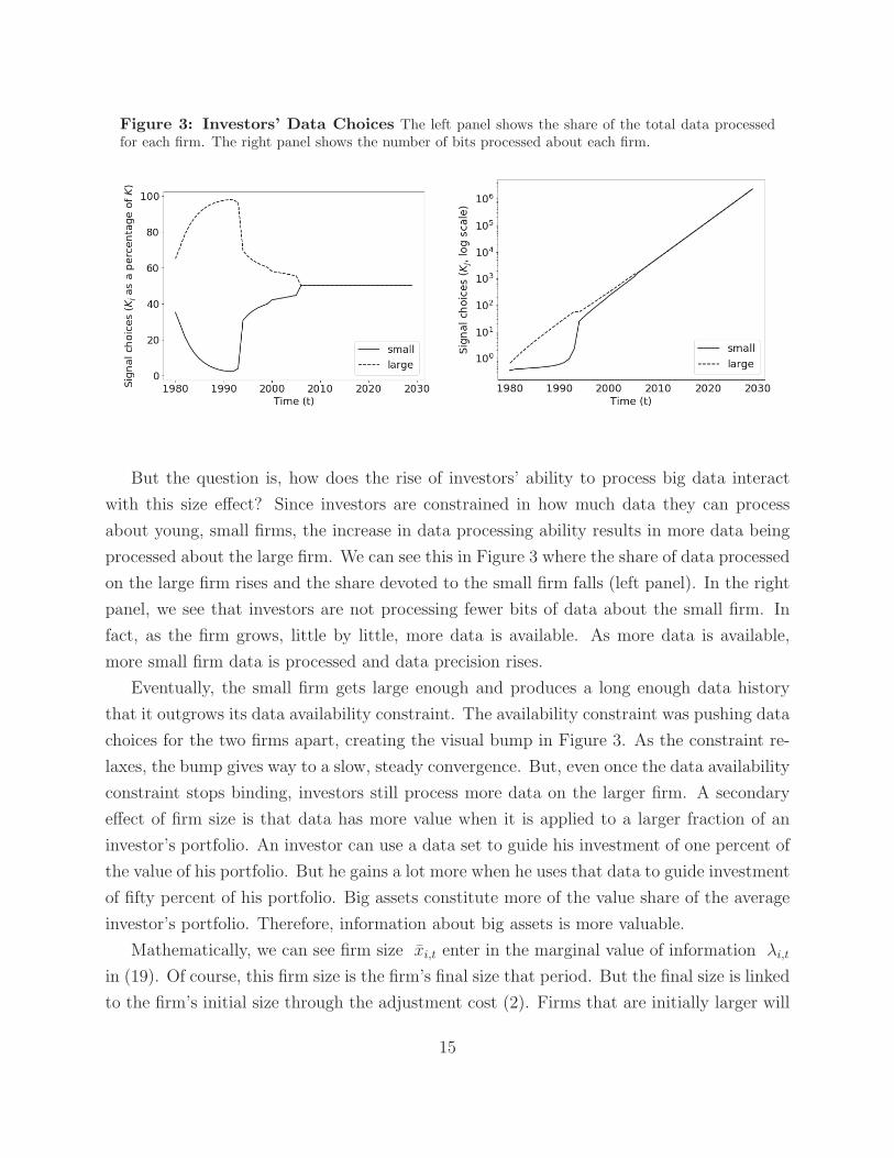
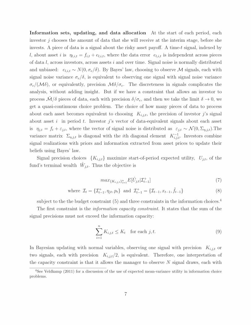
Figure 3: Investors’ Data Choices The left panel shows the share of the total data processedfor each firm. The right panel shows the number of bits processed about each firm.
But the question is, how does the rise of investors’ ability to process big data interact
with this size effect? Since investors are constrained in how much data they can process
about young, small firms, the increase in data processing ability results in more data being
processed about the large firm. We can see this in Figure 3 where the share of data processed
on the large firm rises and the share devoted to the small firm falls (left panel). In the right
panel, we see that investors are not processing fewer bits of data about the small firm. In
fact, as the firm grows, little by little, more data is available. As more data is available,
more small firm data is processed and data precision rises.
Eventually, the small firm gets large enough and produces a long enough data history
that it outgrows its data availability constraint. The availability constraint was pushing data
choices for the two firms apart, creating the visual bump in Figure 3. As the constraint re-
laxes, the bump gives way to a slow, steady convergence. But, even once the data availability
constraint stops binding, investors still process more data on the larger firm. A secondary
effect of firm size is that data has more value when it is applied to a larger fraction of an
investor’s portfolio. An investor can use a data set to guide his investment of one percent of
the value of his portfolio. But he gains a lot more when he uses that data to guide investment
of fifty percent of his portfolio. Big assets constitute more of the value share of the average
investor’s portfolio. Therefore, information about big assets is more valuable.
Mathematically, we can see firm size xi,t enter in the marginal value of information λi,t
in (19). Of course, this firm size is the firm’s final size that period. But the final size is linked
to the firm’s initial size through the adjustment cost (2). Firms that are initially larger will
15
have a larger final size because size adjustment is costly. This larger final size is what makes
λi,t, the marginal value of data, higher.
In the limit, the small firm keeps growing faster than the large firm and eventually catches
up. When the two firms approach the same size, the data processing on both converges to
an equal, but growing amount of data processing.
3.2 Capital costs
The main effect of data is to systematically reduce a firm’s average cost of capital. Recall that
the capital cost is the expected payoff minus the expected price of the asset (Definition 1).
Data does not change the firm’s payoff, but it does change how a share of the firm is priced.
The systematic difference between expected price and payoff is the investor’s compensation
for risk. Investors are compensated for the fact that firm payoffs are unknown, and therefore
buying a share requires bearing risk. The role of data is to help the investor predict that firm
payoff. In doing so, data reduces the compensation for risk. Just like a larger data set lowers
the variance of an econometric estimate, more data in the model reduces the conditional
variance of estimated firm payoffs. An investor who has a more accurate estimate is less
uncertain and bears less risk from holding the asset. The representative investor is willing
to pay more, on average, for a firm that they have good data on. Of course, the data might
reveal problems at the firm that lower the investor’s valuation of it. But on average, more
data is neither to reveal positive nor negative news. What data does on average improve is
the precision and resolution of risk. Resolving the investors’ risk reduces the compensation
the firm needs to pay the investor for bearing that risk, which reduces the firm’s cost of
capital.
Figure 4 shows how the large firm, with its more abundant data, has a lower cost of
capital. With definition 1 in mind, we can think of the cost of capital as the value per share
delivered to investors. The value per share mechanically depends on the expected payout
per share, which may vary across firm size. In order to compare the cost of capital across
firms of different sizes, we normalize firms’ cost of capital with their expected payout per
share.
More abundant data does not reduce the cost of capital evenly and proportionately.
There is a second force at play here. The second force is that firm size matters. Because a
firm is large, it represents a larger share of the investor’s portfolio. In CAPM-speak, large
firms have a higher beta, and therefore need to offer investors a higher risk compensation.
To induce investors to hold lots of a risk, the compensation per unit of risk must rise. To
16
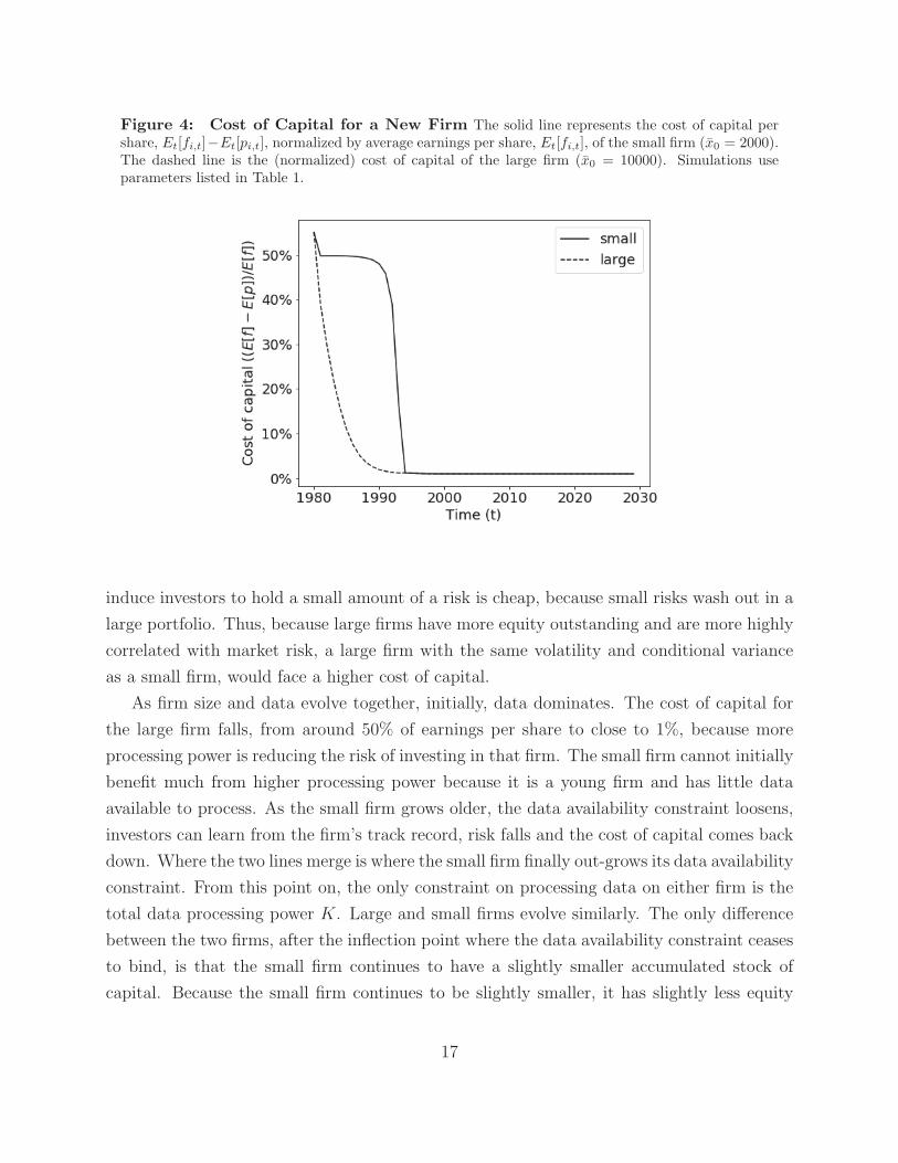
Figure 4: Cost of Capital for a New Firm The solid line represents the cost of capital pershare, Et[fi,t]−Et[pi,t], normalized by average earnings per share, Et[fi,t], of the small firm (x0 = 2000).The dashed line is the (normalized) cost of capital of the large firm (x0 = 10000). Simulations useparameters listed in Table 1.
induce investors to hold a small amount of a risk is cheap, because small risks wash out in a
large portfolio. Thus, because large firms have more equity outstanding and are more highly
correlated with market risk, a large firm with the same volatility and conditional variance
as a small firm, would face a higher cost of capital.
As firm size and data evolve together, initially, data dominates. The cost of capital for
the large firm falls, from around 50% of earnings per share to close to 1%, because more
processing power is reducing the risk of investing in that firm. The small firm cannot initially
benefit much from higher processing power because it is a young firm and has little data
available to process. As the small firm grows older, the data availability constraint loosens,
investors can learn from the firm’s track record, risk falls and the cost of capital comes back
down. Where the two lines merge is where the small firm finally out-grows its data availability
constraint. From this point on, the only constraint on processing data on either firm is the
total data processing power K. Large and small firms evolve similarly. The only difference
between the two firms, after the inflection point where the data availability constraint ceases
to bind, is that the small firm continues to have a slightly smaller accumulated stock of
capital. Because the small firm continues to be slightly smaller, it has slightly less equity
17
outstanding, and a slightly lower cost of capital due to the second force described above.
Once data is abundant, small and large firms converge gradually over time.
3.3 The Evolution of Firms’ Size
In order to understand how big data has changed the size of firms, it is useful to look at how
a large firm and a small firm evolve in this economy. Then, we turn off various mechanisms
in the model to understand what role is played by each of our key assumptions. Once the
various mechanisms are clear, we contrast firm evolution in the 1980’s to the evolution of
firms in the post-2000 period.
Recall that firms have to pay to adjust, relative to their previous size. Since firms’
starting size is small, but rapid growth is costly, firms grow gradually. Figure 5 shows that
both the large and small firms grow. However, the rates at which they grow differ. One
reason growth rates differ is that small firms are further from their optimal size. If this were
the only force at work, small firms would grow by more each period and that growth rate
would gradually decline for both firms, as they approach their optimal size.
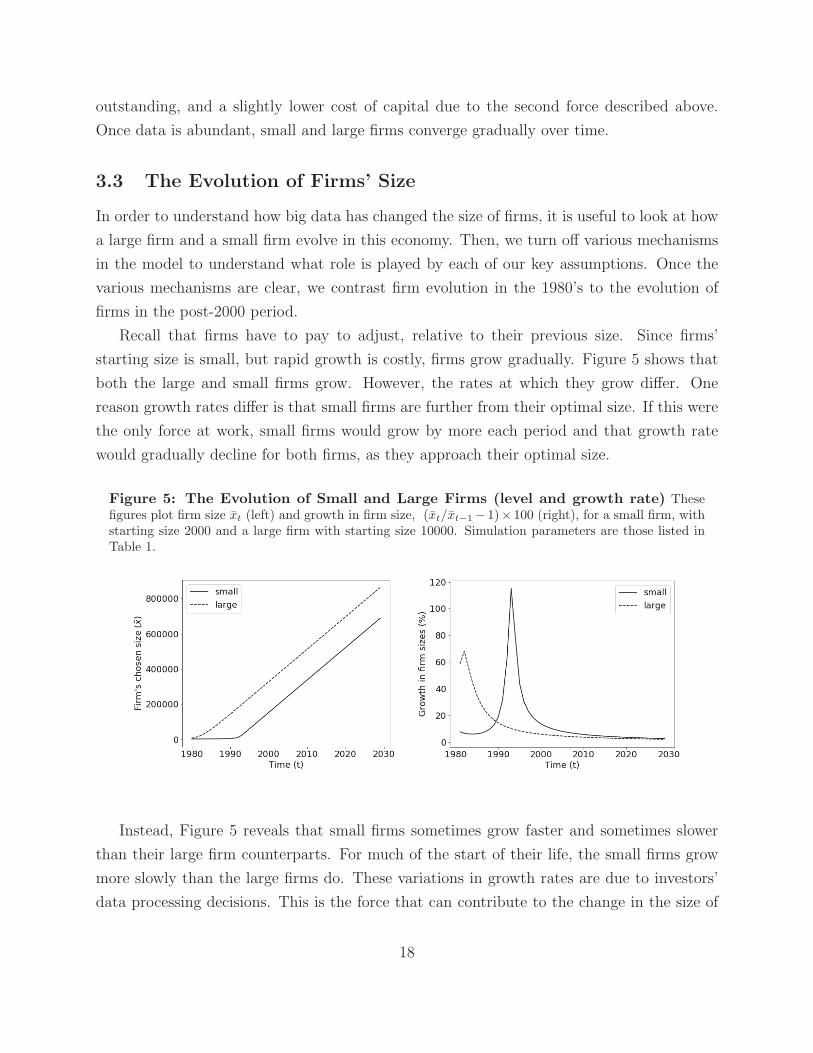
Figure 5: The Evolution of Small and Large Firms (level and growth rate) Thesefigures plot firm size xt (left) and growth in firm size, (xt/xt−1− 1)× 100 (right), for a small firm, withstarting size 2000 and a large firm with starting size 10000. Simulation parameters are those listed inTable 1.
Instead, Figure 5 reveals that small firms sometimes grow faster and sometimes slower
than their large firm counterparts. For much of the start of their life, the small firms grow
more slowly than the large firms do. These variations in growth rates are due to investors’
data processing decisions. This is the force that can contribute to the change in the size of
18
firms.
The level of the size can be interpreted as market capitalization, divided by the expected
price. Since the average price ranges from 7 to 15 in this model, these are firms with zero
to 12 million dollars of market value outstanding. In other words, these are not very large
firms.
The Role of Growing Big Data Plotting firm outcomes over time as in Figure 5 conflates
three forces, all changing over time. The first thing changing over time is that firms are
accumulating capital and growing bigger. The second change is that firms are accumulating
longer data histories, which makes more data for processing available. The third change is
that technology enables investors to process more and more of that data over time. We want
to understand how each of these contributes to our main results. Therefore, we turn off
features of the model one-by-one, and compare the new results to the main results, in order
to understand what role each of these ingredients plays.
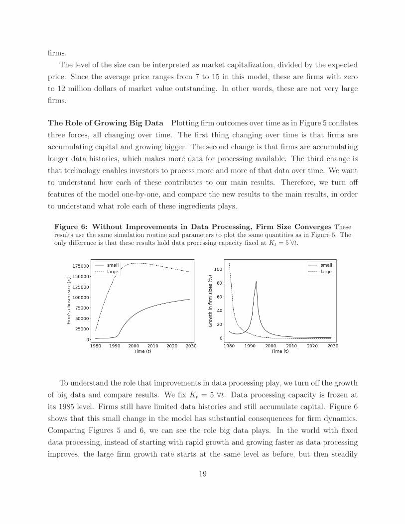
Figure 6: Without Improvements in Data Processing, Firm Size Converges Theseresults use the same simulation routine and parameters to plot the same quantities as in Figure 5. Theonly difference is that these results hold data processing capacity fixed at Kt = 5 ∀t.
To understand the role that improvements in data processing play, we turn off the growth
of big data and compare results. We fix Kt = 5 ∀t. Data processing capacity is frozen at
its 1985 level. Firms still have limited data histories and still accumulate capital. Figure 6
shows that this small change in the model has substantial consequences for firm dynamics.
Comparing Figures 5 and 6, we can see the role big data plays. In the world with fixed
data processing, instead of starting with rapid growth and growing faster as data processing
improves, the large firm growth rate starts at the same level as before, but then steadily
19
declines as the firm approaches is stationary optimal size. We learn that improvements in
data processing are the sources of firm growth in the model and are central to the continued
rapid growth of large firms.
The Role of Limited Data History One might wonder, if large firms attract more data
processing, is that alone producing larger big firms? Is the assumption that small firms have
a limited data history really important for the results? To answer this question, we now turn
off the assumption of limited data history. We maintain the growing data capacity and firm
capital accumulation from the original model.
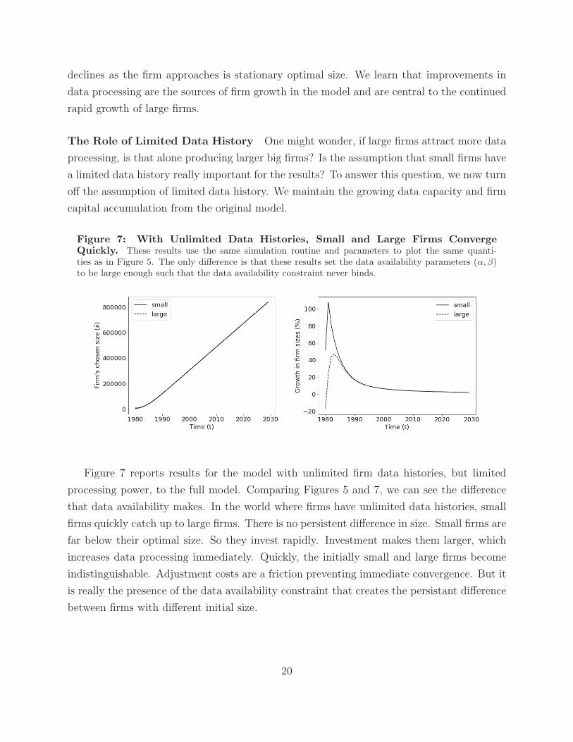
Figure 7: With Unlimited Data Histories, Small and Large Firms ConvergeQuickly. These results use the same simulation routine and parameters to plot the same quanti-ties as in Figure 5. The only difference is that these results set the data availability parameters (α, β)to be large enough such that the data availability constraint never binds.
Figure 7 reports results for the model with unlimited firm data histories, but limited
processing power, to the full model. Comparing Figures 5 and 7, we can see the difference
that data availability makes. In the world where firms have unlimited data histories, small
firms quickly catch up to large firms. There is no persistent difference in size. Small firms are
far below their optimal size. So they invest rapidly. Investment makes them larger, which
increases data processing immediately. Quickly, the initially small and large firms become
indistinguishable. Adjustment costs are a friction preventing immediate convergence. But it
is really the presence of the data availability constraint that creates the persistant difference
between firms with different initial size.
20
Small and Large Firms in the New Millennium So far, the experiment has been
to drop a small firm and a large firm in the economy in 1980 and watch how they evolve.
While this is useful to explaining the model’s main mechanism, it does not really answer the
question of why small firms today struggle more than in the past and why large firms today
are larger than the large firms of the past. To answer these questions, we really want to
compare small and large firms that enter the economy today to small and large firms that
entered in 1980.
To do this small vs. large, today vs. 1980 experiment, we use the same parameters as in
Table 1 and use the same starting size for firms. The only difference is that we start with
more available processing power. Instead of starting Kt at 1, we start it at the 2000 value,
which is about 527.
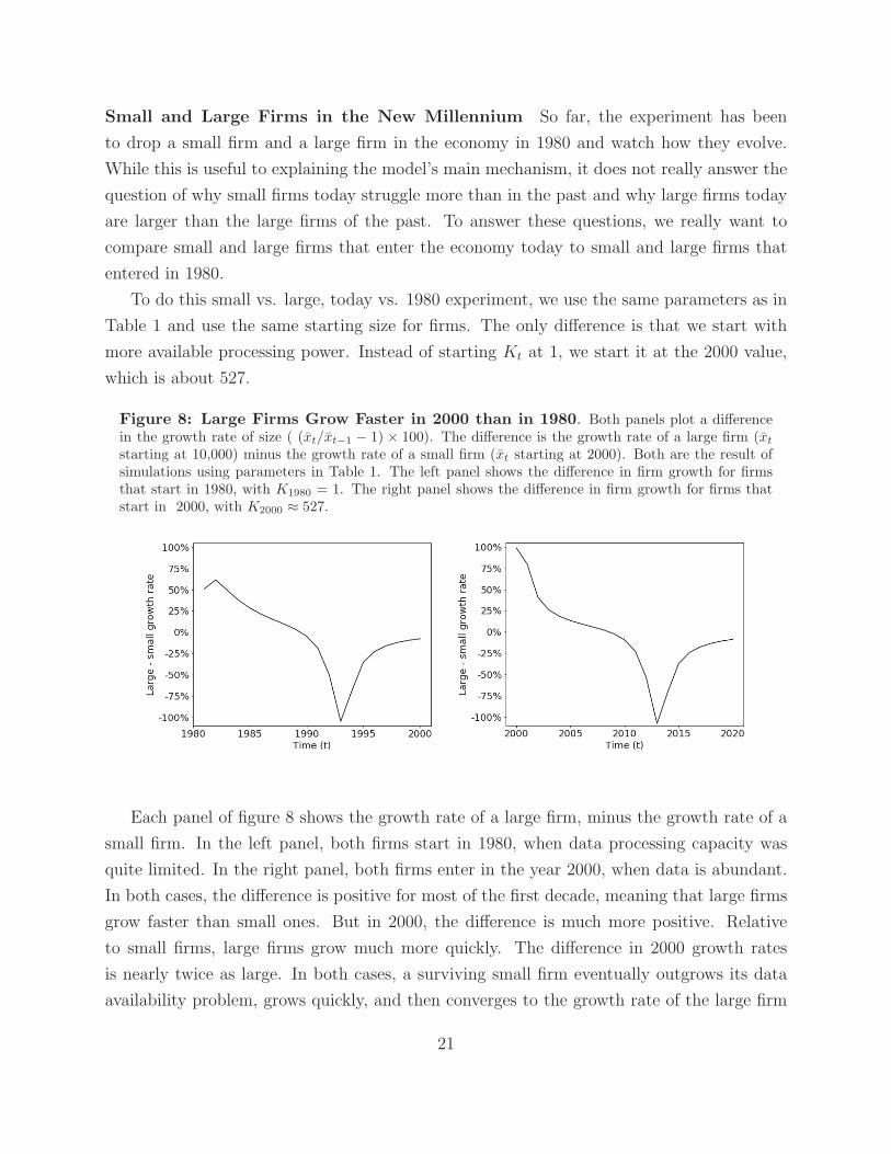
Figure 8: Large Firms Grow Faster in 2000 than in 1980. Both panels plot a differencein the growth rate of size ( (xt/xt−1 − 1) × 100). The difference is the growth rate of a large firm (xt
starting at 10,000) minus the growth rate of a small firm (xt starting at 2000). Both are the result ofsimulations using parameters in Table 1. The left panel shows the difference in firm growth for firmsthat start in 1980, with K1980 = 1. The right panel shows the difference in firm growth for firms thatstart in 2000, with K2000 ≈ 527.
Each panel of figure 8 shows the growth rate of a large firm, minus the growth rate of a
small firm. In the left panel, both firms start in 1980, when data processing capacity was
quite limited. In the right panel, both firms enter in the year 2000, when data is abundant.
In both cases, the difference is positive for most of the first decade, meaning that large firms
grow faster than small ones. But in 2000, the difference is much more positive. Relative
to small firms, large firms grow much more quickly. The difference in 2000 growth rates
is nearly twice as large. In both cases, a surviving small firm eventually outgrows its data
availability problem, grows quickly, and then converges to the growth rate of the large firm
21

(differences converge to 0).
In a model with random shocks and exit, many small firms would not survive. Of course,
for some firms, the possibility of future growth would induce them to hang on, preventing
exit. In a world where large firms gain market share much more rapidly, firms would either
exit, unable to compete, or strive to quickly grow large. This illustrates how data pro-
cessing advances may contribute to the puzzle of missing small firms, by disproportionately
benefiting large firms.
For comparison, we examine the growth rates of large and small firms in the U.S. pre-
1980 and in the period 1980-2007. We end in 2007 so as to avoid measuring real effects of
the financial crisis. For each industry sector and year, we select the top 25% largest firms in
Compustat and call those large firms and select the bottom half of the firm size distribution
to be our small firms. Within these two sets of firms, we compute the growth rates of various
measures of firm size and average them, with an equal weight given to each firm. Then, just
as in the model, we subtract the growth rate of large firms from that of small firms. For
most measures, small firms grow more slowly, and that difference grows later in the sample.
Table 2: Large Firm Growth Minus Small Firm Growth from CompustatFor each industry sector and year, large firms are the top 25% largest firms in Compustat; small firmsare the bottom half of the firm size distribution. Growth rate is the annual log-difference. Reportedfigures are equal-weighted averages of growth rates over firms and years.
prior to 1980 1980 - 2007
Assets 2.1% 8.2%Investment 14.2% 16.0%Assets with Intangibles 0.3% 1.1%Capital Stock -0.9% 3.7%Sales 1.4% 2.4%Market Capitalization 1.1% 8.9%
At times, the magnitudes of the model’s growth rates are quite large, compared to the
data. Of course, the data is averaged over many years and many firms at different points in
their life cycle. This smoothes out some of the extremes in the data. If we average the firm
growth in our model from 1980-1985, for firms that enter in 1980, we get 39.5% for large
firms and 7.3% for small firms, a difference of 32.2%. If we average firm growth in our model
from 2000-2005, for firms that enter in 2000, we get 59.9% for large firms and 7.3% for small
firms, a difference of 52.6%.
While it is not unheard of for a small firm to double in size, some of this magnitude
22
undoubtedly reflects some imprecision of our current numerical example vis-a-vis the data.
A larger adjustment cost, or a labor hiring delay, would help to moderate the extremes of firm
size growth. The results also miss many aspects of the firm environment that have changed
in the last four decades. The type of firms entering in the last few years are quite different
than firms of prior years. They have different sources of revenue and assets that might be
harder to value. Firm financing has changed, with a shift toward internal financing. Venture
capital funding has become more prevalent and displaced equity funding for many firms,
early in their life cycle. All of these forces would moderate the large effect we document
here.
Our results only show that big data is a force with some potential. There is a logical way
in which the growth of big data and the growth of large firms is connected. This channel
has the potential to be quantitatively powerful. The role of big data in firms is thus a topic
ripe for further exploration.
4 Discussion
In this model, there is a one-to-one correspondence between projects and firms. Investors
gather information about the firm and smaller firms have smaller amounts of information.
This then feeds back into real investments of each firm in its single project, and determines
the firm/project size distribution. As such, information processing and big data helps a
small firm less, even if it is investing in a well known technology (for instance, the nth firm
to drill an oil well). We think this is a reasonable assumptions for publicly listed firms, since
information about the firm is both about its track record as well as the quality of its project.
The investors have a harder time accessing the survival probability of a firm with no track
record relative to a well established firm in a highly competitive industry, which is why we
find our information assumption relevant even in such settings.
We should note that our model is not best suited to speak to firm entry. For instance, a
new class of online firms have emerged who use big data to facilitate capital markets’ access
to an under-served segment of population, such as personal loans to people with very low
credit scores. Such firms are often small, but they have only emerged as a by product of big
data availability. This trend is fascinating in its own right, yet is outside the scope of our
paper.
In the context of the model, firms are equity financed. This implies that their real
investment and thus their cash flow is determined by firms’ cost of accessing external capital
23
markets. Financing is costly for firms since investors require an equity premium to hold
firms’ risky shares. However, since more data is available about large firms, big data reduces
the asymmetric information friction relatively more for big firms compared to small firms.
Cheaper access to external capital markets reduces large firms’ cost of capital and accelerates
their growth. On the other hand, small firms growth is initially stagnant. However, once
they become sufficiently large, their access to capital markets improve as well, and their
growth rate picks up. This is consistent with information asymmetries being a short-horizon
notion.
5 Conclusion
Big data is transforming the modern economy. While many economists have used big data,
fewer think about how the use of data by others affects market outcomes. This paper starts to
explore the ways in which big data might be incorporated in modern economic and financial
theory. One way that big data is used is to help financial market participants make more
informed choices about the firms in which they invest. These investment choices affect the
prices, cost of capital, and investment decisions of these firms. We set up a very simple
model to show how such big data choices might be incorporated and one way in which the
growth of big data might affect the real economy. But this is only a modest first step.
One might also consider how firms themselves use data, to refine their products, to
broaden their customer market, or to increase the efficiency of their operations. Such data,
produced as a by-product of economic activity, might also favor the large firms whose abun-
dant economic activity produces abundant data.
Another step in a big-data agenda would be to consider the sale of data. In many
information models, we think of signals that are observed and then embedded in one’s
knowledge, not easily or credibly transferable. However data is an asset that can be bought,
sold and priced on a market. How do markets for data change firms choices, investments,
evolution and their valuations as firms? It is true that data intermediaries like Foursquare
or Amazon help small businesses benefit from each others’ data. At the same time, these
intermediaries retain control of the data and extract rents from firms that use it. A firm
that has its own customer data clearly has a real advantage. Whether an intermediary can
find a way for small firms to collectively leverage their data, in a way that mimics a large
firm advantage, remains to be seen.
Finally, if data is a storable, sellable, priced asset, then investment in data should be
24

valued just as if it were investment in a physical asset. Understanding how to price data as
an asset might help us to better understand the valuations of new-economy firms and better
measure aggregate economic activity.
25

References
Akcigit, U. and W. Kerr (2017): “Growth through Heterogeneous Innovations,” Journal of
Political Economy, forthcoming.
Asriyan, V. and V. Vanasco (2014): “Informed Intermediation over the Cycle,” Stanford Work-
ing Paper.
Bai, J., T. Philippon, and A. Savov (2016): “Have Financial Markets Become More Informa-
tive?” Journal of Financial Economics, 122 35), 625–654.
Begenau, J. and J. Salomao (2018): “Firm Financing over the Business Cycle,” Review of
Financial Studies, forthcoming.
Bernhardt, D., B. Hollifield, and E. Hughson (1995): “Investment and insider trading,”
The Review of Financial Studies, 8, 501–543.
Biais, B., T. Foucault, and S. Moinas (2015): “Equilibrium Fast Trading,” Journal of Finan-
cial Economics, 116, 292–313.
Cooley, T. F. and V. Quadrini (2001): “Financial Markets and Firm Dynamics,” American
Economic Review, 91, 1286–1310.
Cover, T. and J. Thomas (1991): Elements of information theory, John Wiley and Sons, New
York, New York, first ed.
Davis, S. J. and J. Haltiwanger (2015): “Dynamism Diminished: The Role of Credit Condi-
tions,” in progress.
Fang, L. and J. Peress (2009): “Media Coverage and the Cross-section of Stock Returns,” The
Journal of Finance, 64, 2023–2052.
Farboodi, M., A. Matray, and L. Veldkamp (2017): “Where Has All the Big Data Gone?”
Working Paper, Princeton University.
Glode, V., R. Green, and R. Lowery (2012): “Financial Expertise as an Arms Race,” Journal
of Finance, 67, 1723–1759.
Gomes, J. F. (2001): “Financing Investment,” The American Economic Review, 91, pp. 1263–
1285.
Grossman, S. and J. Stiglitz (1980): “On the impossibility of informationally efficient markets,”
American Economic Review, 70(3), 393–408.
26
Hennessy, C. A. and T. M. Whited (2007): “How Costly Is External Financing? Evidence
from a Structural Estimation,” The Journal of Finance, LXII.
Hennessy, J. and D. Patterson (2011): Computer Architecture, Elsevier.
Kacperczyk, M., J. Nosal, and L. Stevens (2015): “Investor Sophistication and Capital
Income Inequality,” Imperial College Working Paper.
Kacperczyk, M., S. Van Nieuwerburgh, and L. Veldkamp (2016): “A Rational Theory of
Mutual Funds’ Attention Allocation,” Econometrica, 84(2), 571–626.
Kozeniauskas, N. (2017): “Technical Change and Declining Entrepreneurship,” Working Paper,
New York University.
Maksimovic, V., A. Stomper, and J. Zechner (1999): “Capital structure, information acqui-
sition and investment decisions in an industry framework,” Review of Finance, 2, 251–271.
Ozdenoren, E. and K. Yuan (2008): “Feedback effects and asset prices,” The journal of finance,
63, 1939–1975.
Van Nieuwerburgh, S. and L. Veldkamp (2010): “Information acquisition and under-
diversification,” Review of Economic Studies, 77 (2), 779–805.
Veldkamp, L. (2011): Information choice in macroeconomics and finance, Princeton University
Press.
27

A Proofs
A.1 Useful notation, matrices and derivatives
All the following matrices are diagonal with ii entry given by:
1. Average signal precision: (Σ−1
η,t)ii = Ki,t, where Ki,t ≡∫
Ki,j,tdj.
2. Precision of the information prices convey about shock i: (Σ−1
p,t )ii =K2
i,t
ρ2σx= σ−1
i,p,t
3. Precision of posterior belief about shock i for an investor j is σ−1
i,j,t, which is equivalent to
(Σ−1
j,t )ii = (Σ−1 +Σ−1
η,j,t +Σ−1
p,t )ii = σ−1
i +Ki,j,t +K2
i,t
ρ2σx= σ−1
i,j,t (22)
4. Average posterior precision of shock i: σ−1
i,t ≡ σ−1
i + Ki,t +K2
i,t
ρ2σx. The average variance is therefore
(Σt)ii = [(
σ−1
i + Ki,t +K2
i,t
ρ2σx
)
]−1 = σi,t.
5. Ex-ante mean and variance of returns: Using Lemma 1 and the coefficients given by (33), (34) and(35), we can write the return as:
ft − ptrt = (I −Bt)(ft − µ)− Ctxt + ρΣtxt
= Σt
[
Σ−1(ft − µ) + ρ
(
I +1
ρ2σxΣ−1
′
η,t
)
xt
]
+ ρΣtxt.
This expression is a constant plus a linear combination of two normal variables, which is also a normalvariable. Therefore, we can write
ft − ptrt = V1/2t ut + wt, (23)
where ut is a standard normally distributed random variable ut ∼ N(0, I), and wt is a non-randomvector measuring the ex-ante mean of excess returns
wt ≡ ρΣtxt. (24)
and Vt is the ex-ante variance matrix of excess returns:
Vt ≡ Σt
[
Σ−1 + ρ2σx
(
I +1
ρ2σxΣ−1
′
η,t
)(
I +1
ρ2σxΣ−1
′
η,t
)
′
]
Σt
= Σt
[
Σ−1 + ρ2σx
(
I +1
ρ2σx(Σ−1
′
η,t + Σ−1
η,t) +1
ρ4σ2x
Σ−1′
η,t Σ−1
η,t
)]
Σt
= Σt
[
Σ−1 + ρ2σxI + (Σ−1′
η,t + Σ−1
η,t) +1
ρ2σxΣ−1
′
η,t Σ−1
η,t
]
Σt
= Σt
[
ρ2σxI + Σ−1′
η,t +Σ−1 + Σ−1
η,t +Σ−1
p,t
]
Σt
= Σt
[
ρ2σxI + Σ−1′
η,t + Σ−1
t
]
Σt.
The first line uses E[xtx′
t] = σxI and E[(ft −µ)(ft −µ)′] = Σ, the fourth line uses (36) and the fifthline uses Σ−1
t = Σ−1 +Σ−1
p,t + Σ−1
η,t .
28
This variance matrix Vt is a diagonal matrix. Its diagonal elements are:
(Vt)ii = (Σt
[
ρ2σxI + Σ−1
η,t + Σ−1
t
]
Σt)ii
= σi,t[1 + (ρ2σx + Ki,t)σi,t]. (25)
A.2 Solving the Model
Step 1: Portfolio Choices From the FOC, the optimal portfolio is chosen by investor j is
q∗j,t =1
ρΣ−1
j,t (Ej,t[ft]− ptrt). (26)
where Ej,t[ft] and Σj,t depend on the skill of the investor.Next, we compute the portfolio of the average investor.
q ≡
∫
q∗j,tdj =1
ρ
∫
Σ−1
j,t (Ej,t[ft]− ptrt)dj
=1
ρ
(∫
Σ−1
η,j,tηj,tdj +Σ−1
p,tηp,t + Σ−1
t (µ− ptrt)
)
=1
ρ
(
Σ−1
η,tft +Σ−1
p,tηp,t + Σ−1
t (µ− ptrt))
, (27)
where the fourth equality uses the fact that average noise of private signals is zero.
Step 2: Clearing the asset market and computing expected excess return Lemma1 describes the solution to the market-clearing problem and derives the coefficients At, Bt, and Ct in thepricing equation. The equilibrium price, along with the random signal realizations determines the interimexpected return (Ej,t[ft] − ptrt). But at the start of the period, the equilibrium price and one’s realizedsignals are not known. To compute beginning-of-period utility, we need to know the ex-ante expectation andvariance of this interim expected return.
The interim expected excess return can be written as: Ej,t[ft] − ptrt = Ej,t[ft] − ft + ft − ptrt andtherefore its variance is:
Vt[Ej,t[ft]− ptrt] = Vt[Ej,t[ft]− ft] + Vt[ft − ptrt] + 2Covt[Ej,t[ft]− ft, ft − ptrt]. (28)
Combining (12) with the definitions ηj,t = ft+ εj,t and ηp,t = ft+ εp,t, we can compute expectation errors:
Ej,t[ft]− ft = Σj,t
[
(Σ−1µ+ (Σ−1
η,j,t +Σ−1
p,t )ft +Σ−1
η,j,tεj,t +Σ−1
p,tεp,t]
− ft
= Σj,t
[
−Σ−1(ft − µ) + Σ−1
η,j,tεj,t +Σ−1
p,tεp,t]
Computing the expectation, we obtain Et[Ej,t[ft]− ft] = Σj,tΣ−1
j,t µ− µ = 0 and its variance is Vt[Ej,t[ft]−
ft] = Σj,t
[
Σ−1 +Σ−1
η,j,t +Σ−1
p,t
]
Σ′
j,t = Σj,t.From (23) we know that Vt[ft − ptrt] = Vt. To compute the covariance term, we can rearrange the
definition of ηp,t to get ptrt = Btηp,t +At −Btµ and ηp,t = ft + εp,t to write
ft − ptrt = (I −Bt)ft −At −Btεp,t +Btµ (29)
= ρΣtxt + ΣtΣ−1(ft − µ)− (I − ΣtΣ
−1)εp,t (30)
29

where the second line comes from substituting the coefficients At and Bt from Lemma 1. Since the constantρΣtxt does not affect the covariance, we can write
Covt[Ej,t[ft]− ft, ft − ptrt] = Cov[−Σj,tΣ−1(ft − µ) + Σj,tΣ
−1
p,tεp,t, ΣtΣ−1(ft − µ)− (I − ΣtΣ
−1)εp,t]
= −Σj,tΣ−1ΣΣ−1Σt − Σj,tΣ
−1
p,tΣp,t(I − Σ−1Σt)]
= −Σj,tΣ−1Σt − Σj,t(I − Σ−1Σt) = −Σj,t
Substituting the three variance and covariance terms into (28), we find that the variance of excess returnis Vt[Ej,t[ft] − ptrt] = Σj,t + Vt − 2Σj,t = Vt − Σj,t. Note that this is a diagonal matrix. Substituting the
expressions (25) and (22) for the diagonal elements of Vt and Σj,t we have
(Vt[Ej,t[ft]− ptrt])ii = (Vt − Σj,t)ii = (σi,t − σi,j,t) + (ρ2σx + Ki,t)σ2
i,t
In summary, the excess return is normally distributed as Ej,t[ft]− ptrt ∼ N (wt, Vt − Σj,t).
Step 3: Compute ex-ante expected utility Ex-ante expected utility for investor j is Uj,t =
Et
[
ρEj,t[Wj,t]−ρ2
2Vj,t[Wj,t]
]
. In period 2, the investor has chosen his portfolio and the price is in his infor-
mation set, therefore the only payoff-relevant, random variable is ft. We substitute the budget constraint inthe optimal portfolio choice from (26) and take expectation and variance conditioning on Ej,t[ft] and Σj,t
to obtain Uj,t = ρrtWt +1
2Et[(Ej,t[ft]− ptrt)
′Σ−1
j,t (Ej,t[ft]− ptrt)].
Define mt ≡ Σ−1/2j,t (Ej,t[ft] − ptrt) and note that mt ∼ N (Σ
−1/2j,t wt, Σ
−1/2j,t VtΣ
−1/2′
j,t − I). The secondterm in the Ui,t is equal to E[m′
tmt], which is the mean of a non-central Chi-square. Using the formula, ifmt ∼ N(E[mt], V ar[mt]), then E[m′
tmt] = tr(V ar[mt]) + E[mt]′E[mt], we get
Uj,t = ρrtWt +1
2tr(Σ
−1/2j,t V Σ
−1/2′
j,t − I) +1
2w′
tΣ−1
j,twt = ρrtWt +1
2tr(Σ−1
j,t V )− tr(I) +1
2w′
tΣ−1
j,twt.
Finally, we substitute the expressions for Σ−1
j,t and wt from (22) and (24):
Uj,t = ρrtWt −N
2+
1
2
N∑
i=1
(
σ−1
i +Ki,j,t +K2
i,t
ρ2σx
)
(Vt)ii +ρ2
2
N∑
i=1
x2
i,tσ2
i,t
(
σ−1
i +Ki,j,t +K2
i,t
ρ2σx
)
=1
2
N∑
i=1
Ki,j,t[(Vt)ii + ρ2x2
i,tσ2
i,t] + ρrtWt −N
2+
1
2
N∑
i=1
(
σ−1
i +K2
i,t
ρ2σx
)
[(Vt)ii + ρ2x2
i,tσ2
i,t]
=1
2
N∑
i=1
Ki,j,tλi,t + constant (31)
λi,t = σi,t[1 + (ρ2σx + Ki,t)σi,t] + ρ2x2
i,tσ2
i,t (32)
where the weights λi,t are given by the variance of expected excess return (Vt)ii from (25) plus a term thatdepends on the supply of the risk.
Step 4: Information choices The attention allocation problem maximizes ex-ante utility in (31)subject to the information capacity, data availability and no-forgetting constraints (17), (18) and (11).Observe that λi,t depends only on parameters and on aggregate average precisions. Since each investorhas zero mass within a continuum of investors, he takes λi,t as given. Since the constant is irrelevant,the optimal choice maximizes a weighted sum of attention allocations, where the weights are given by λi,t
30
(equation (19)), subject to a constraint on an un-weighted sum. This is not a concave objective, so a first-order approach will not deliver a solution. A simple variational argument reveals that allocating all capacityto the risk(s) with the highest λi,t achieves the maximum utility. For a formal proof of this result, see VanNieuwerburgh and Veldkamp (2010). Thus, the solution is given by: Ki,j,t = Kt if λi,t = maxk λk,t, andKi,j,t = 0, otherwise. There may be multiple risks i that achieve the same maximum value of λi,t. In thatcase, the manager is indifferent about how to allocate attention between those risks. We focus on symmetricequilibria.
A.3 Proofs
Proof of Lemma 1
Proof. Following Admati (1985), we know that the equilibrium price takes the following form ptrt =At +Bt(ft − µ) + Ctxt where
At = µ− ρΣtxt (33)
Bt = I − ΣtΣ−1 (34)
Ct = −ρΣt
(
I +1
ρ2σxΣ−1
′
η,t
)
(35)
and therefore the price is given by ptrt = µ+Σt
[
(Σ−1
t − Σ−1)(ft − µ)− ρ(xt + xt)−1
ρσxΣ−1
′
η,t xt
]
. Further-
more, the precision of the public signal is
Σ−1
p,t ≡(
σxB−1
t CtC′
tB−1
′
t
)
−1
=1
ρ2σxΣ−1
′
η,t Σ−1
η,t (36)
Proof of Lemma 2 See Kacperczyk et. al (2016).
A.4 Firm Volatility Data
The introduction of our paper claims that differential trends in the volatility of large and small firms’ earningsis not a plausible explanation for the different trends in the cost of capital. To support this claim, we explorewhether the volatility of large and small firms has diverged. We find some fluctuations, but no consistenttrend in the difference.
Our volatility measure is based on the annual growth rate in earnings calculated at the firm level fromquarterly CRSP/Computat data from 1960 - 2016. Earnings are constructed by multiplying basic earningsper share, excluding extraordinary items (EPS) by the number of shares used to calculate EPS. We measurethe volatility of earnings growth as the rolling standard deviation over the past 20 quarters. The firms aresplit by size in a number of ways: firstly, the firms in the sample are split by whether or not they are (at thattime) a member of the S&P500 index. Secondly, we split firms by whether or not they were in the top halfof the earnings distribution in each quarter. Lastly, we consider only firms in the bottom and top quartilesof the earnings distribution. In the plots below, the dashed lines are the median volatility, whilst the solidline is the trend extracted from this series using a HP filter, with λ = 1600.
31
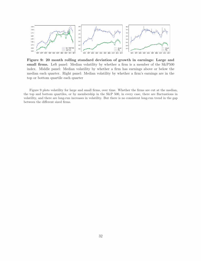
Figure 9: 20 month rolling standard deviation of growth in earnings: Large andsmall firms. Left panel: Median volatility by whether a firm is a member of the S&P500index. Middle panel: Median volatility by whether a firm has earnings above or below themedian each quarter. Right panel: Median volatility by whether a firm’s earnings are in thetop or bottom quartile each quarter
Figure 9 plots volatility for large and small firms, over time. Whether the firms are cut at the median,the top and bottom quartiles, or by membership in the S&P 500, in every case, there are fluctuations involatility, and there are long-run increases in volatility. But there is no consistent long-run trend in the gapbetween the different sized firms.
32