Embed Size (px)
Citation preview
7/27/2019 Big Data Analysis using Python
http://slidepdf.com/reader/full/big-data-analysis-using-python 1/62
Published in:Reinhard Leidl and Alexander K. Hartmann (eds.)Modern Computational Science 2012 – OptimizationLecture Notes from the 4th International Summer School BIS-Verlag, Oldenburg, 2012. ISBN 978-3-8142-2269-1
Basic Data Analysis and More – A Guided TourUsing python
Oliver Melchert Institute of Physics Faculty of Mathematics and Science Carl von Ossietzky Universit¨ at Oldenburg D-26111 Oldenburg Germany
Abstract. In these lecture notes, a selection of frequently required statistical toolswill be introduced and illustrated. They allow to post-process data that stem from,e.g., large-scale numerical simulations (aka sequence of random experiments). Froma point of view of data analysis, the concepts and techniques introduced here are of general interest and are, at best, employed by computational aid. Consequently, anexemplary implementation of the presented techniques using the python program-ming language is provided. The contents of these lecture notes is rather selectiveand represents a computational experimentalist’s view on the subject of basic data
analysis, ranging from the simple computation of moments for distributions of ran-dom variables to more involved topics such as hierarchical cluster analysis and theparallelization of python code.
Note that in order to save space, all python snippets presented in the follow-ing are undocumented. In general, this has to be considered as bad program-ming style. However, the supplementary material, i.e., the example programsyou can download from the MCS homepage, is well documented (see Ref. [1]).
1
a r X i v : 1 2 0 7 . 6
0 0 2
v 1
[ p h y s i c s . d a
t a - a n ] 2 5 J u l 2
0 1 2
7/27/2019 Big Data Analysis using Python
http://slidepdf.com/reader/full/big-data-analysis-using-python 2/62
Basic data analysis (Melchert)
Contents
1 Basic python: selected features . . . . . . . . . . . . . . . . 2
2 Basic data analysis . . . . . . . . . . . . . . . . . . . . . . . 6
2.1 Distribution of random variables . . . . . . . . . . . . . . . 6
2.2 Histograms . . . . . . . . . . . . . . . . . . . . . . . . . . . 21
2.3 Bootstrap resampling . . . . . . . . . . . . . . . . . . . . . 25
2.4 The chi-square test . . . . . . . . . . . . . . . . . . . . . . . 273 Object oriented programming in python . . . . . . . . . . . 31
3.1 Implementing an undirected graph . . . . . . . . . . . . . . 32
3.2 A simple histogram data structure . . . . . . . . . . . . . . 38
4 Increase your efficiency using Scientific Python (scipy) . 42
4.1 Basic data analysis using scipy . . . . . . . . . . . . . . . . 42
4.2 Least-squares parameter estimation using scipy . . . . . . 45
4.3 Maximum-likelihood parameter estimation using scipy . . 47
4.4 Hierarchical cluster analysis using scipy . . . . . . . . . . . 51
5 Struggling for speed . . . . . . . . . . . . . . . . . . . . . . 555.1 Combining C and python (Cython) . . . . . . . . . . . . . . 55
5.2 Parallel computing and python . . . . . . . . . . . . . . . . 58
6 Further reading . . . . . . . . . . . . . . . . . . . . . . . . . 61
1 Basic python: selected features
Although python syntax is almost as readable as pseudocode (allowing for an intuitive
understanding of the code-snippets listed in the present section), it might be usefulto discuss a minimal number of its features, needed to fully grasp the examples andscripts in the supplementary material (see Ref. [1]). In this regard, the intentionof the present notes is not to demonstrate every nut, bolt and screw of the python
programming language, it rather illustrates some basic data structures and showshow to manipulate them. To get a more comprehensive introduction to the python
programming language, Ref. [2] is a good starting point.There are two elementary data structures which one should be aware of when
using python: lists and dictionaries . Subsequently, the use of these is illustrated bymeans of the interactive python mode. One can enter this mode by simply typing
python on the command line.
Lists. A list is denoted by a pair of square braces. The list elements are indexed byinteger numbers, where the smallest index has value 0. Generally speaking, lists cancontain any kind of data. Some basic options to manipulate lists are shown below:
7/27/2019 Big Data Analysis using Python
http://slidepdf.com/reader/full/big-data-analysis-using-python 3/62
1 Basic python: selected features
1 >>> ## set up an empty list
2 ... a=[]
3 >>> ## set up a list containing integers
4 ... a=[4,1]
5 >>> ## append a further element to the list
6 ... a.append(2)
7 >>> ## print the list and the length of the list
8 ... print "list=",a,"length=",len(a)
9 list= [4, 1, 2] length= 3
10 >>> ## lists are circular, list has indices 0...len(a)-111 ... print a[0], a[len(a)-1], a[-1]
12 4 2 2
13 >>> ## print a slice of the list (upper bound is exclusive)
14 ... print a[0:2]
15 [4, 1]
16 >>> ## loop over list elements
17 ... for element in a:
18 ... print element,
19 ...
20 4 1 221 >>> ## the command range() generates a special list
22 ... print range(3)
23 [0, 1, 2]
24 >>> ## loop over list elements (alternative)
25 ... for i in range(len(a)):
26 ... print i, a[i]
27 ...
28 0 4
29 1 1
30 2 2
Dictionaries. A dictionary is an unordered set of key:value pairs, surrounded bycurled braces. Therein, the keys serve as indexes to access the associated values of the dictionary. Some basic options to manipulate dictionaries are shown below
1 >>> ## set up an empty dictionary
2 ... m =
3 >>> ## set up a small dictionary
4 ... m = ’a’:[1,2]
5 >>> ## add another key:value-pair
6 ... m[’b’]=[8,0]7 >>> ## print the full dictionary
8 ... print m
9 ’a’: [1, 2], ’b’: [8, 0]
10 >>> ## print only the keys/values
7/27/2019 Big Data Analysis using Python
http://slidepdf.com/reader/full/big-data-analysis-using-python 4/62
Basic data analysis (Melchert)
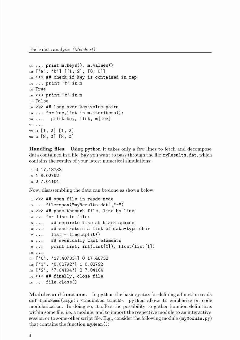
11 ... print m.keys(), m.values()
12 [’a’, ’b’] [[1, 2], [8, 0]]
13 >>> ## check if key is contained in map
14 ... print ’b’ in m
15 True
16 >>> print ’c’ in m
17 False
18 >>> ## loop over key:value pairs
19 ... for key,list in m.iteritems():
20 ... print key, list, m[key]21 ...
22 a [1, 2] [1, 2]
23 b [8, 0] [8, 0]
Handling files. Using python it takes only a few lines to fetch and decomposedata contained in a file. Say you want to pass through the file myResults.dat, whichcontains the results of your latest numerical simulations:
1 0 17.48733
2 1 8.02792
3 2 7.04104
Now, disassembling the data can be done as shown below:
1 >>> ## open file in reade-mode
2 ... file=open("myResults.dat","r")
3 >>> ## pass through file, line by line
4 ... for line in file:
5 ... ## separate line at blank spaces
6 ... ## and return a list of data-type char
7 ... list = line.split()
8 ... ## eventually cast elements9 ... print list, int(list[0]), float(list[1])
10 ...
11 [’0’, ’17.48733’] 0 17.48733
12 [’1’, ’8.02792’] 1 8.02792
13 [’2’, ’7.04104’] 2 7.04104
14 >>> ## finally, close file
15 ... file.close()
Modules and functions. In python the basic syntax for defining a function readsdef funcName(args): <indented block>. python allows to emphasize on codemodularization. In doing so, it offers the possibility to gather function definitionswithin some file, i.e. a module, and to import the respective module to an interactivesession or to some other script file. E.g., consider the following module ( myModule.py)that contains the function myMean():
7/27/2019 Big Data Analysis using Python
http://slidepdf.com/reader/full/big-data-analysis-using-python 5/62
1 Basic python: selected features
1 def myMean(array):
2 return sum(array)/float(len(array))
Within an interactive session this module might be imported as shown below
1 >>> import myModule
2 >>> myModule.myMean(range(10))
3 4.5
4 >>> sqFct = lambda x : x*x
5 >>> myModule.myMean(map(sqFct,range(10)))
6 28.5
This example also illustrates the use of namespaces in python: the function myModule() is contained in an external module and must be imported in orderto be used. As shown above, the function can be used if the respective modulename is prepended. An alternative would have been to import the function di-rectly via the statement from myModule import myMean. Then the simpler state-ment myMean(range(10)) would have sufficed to obtain the above result. Further-more, simple functions can be defined “on the fly” by means of the lambda statement.Line 4 above shows the definition of the function sqFct, a lambda function that re-
turns the square of a supplied number. In order to apply sqFct to each element ina given list, the map(sqFct,range(10)) statement, equivalent to the list comprehen-sion [sqFct(el) for el in range(10)] (i.e. an inline looping construct), might beused.
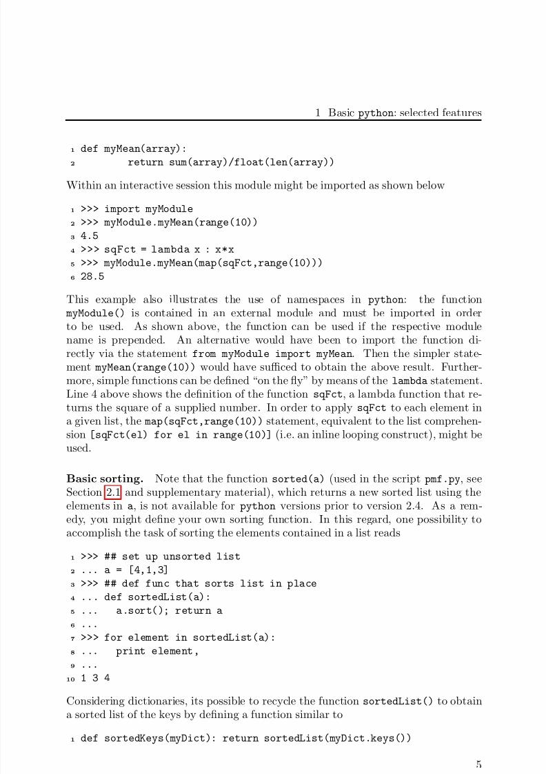
Basic sorting. Note that the function sorted(a) (used in the script pmf.py, seeSection 2.1 and supplementary material), which returns a new sorted list using theelements in a, is not available for python versions prior to version 2.4. As a rem-edy, you might define your own sorting function. In this regard, one possibility toaccomplish the task of sorting the elements contained in a list reads
1 >>> ## set up unsorted list
2 ... a = [4,1,3]
3 >>> ## def func that sorts list in place
4 ... def sortedList(a):
5 ... a.sort(); return a
6 ...
7 >>> for element in sortedList(a):
8 ... print element,
9 ...
10 1 3 4
Considering dictionaries, its possible to recycle the function sortedList() to obtaina sorted list of the keys by defining a function similar to
1 def sortedKeys(myDict): return sortedList(myDict.keys())
7/27/2019 Big Data Analysis using Python
http://slidepdf.com/reader/full/big-data-analysis-using-python 6/62
Basic data analysis (Melchert)
As remark, note that python uses Timsort [3], a hybrid sorting algorithm based onmerge sort and insertion sort [14].
To sum up, python is an interpreted (no need for compiling) high-level program-ming language with a quite simple syntax. Using python, it is easy to write modulesthat can serve as small libraries. Further, a regular python installation comes with anelaborate suite of general purpose libraries that extend the functionality of python andcan be used out of the box. These are e.g., the random module containing functionsfor random number generation, the gzip module for reading and writing compressedfiles, the math module containing useful mathematical functions, the os module pro-
viding a cross-platform interface to the functionality of most operating systems, andthe sys module containing functions that interact with the python interpreter.
2 Basic data analysis
2.1 Distribution of random variables
Numerical simulations, performed by computational means, can be considered asbeing random experiments , i.e., experiments with outcome that is not predictable.For such a random experiment, the sample space Ω specifies the set of all possible
outcomes (also referred to as elementary events ) of the experiment. By means of thesample space, a random variable X (accessible during the random experiment), canbe understood as a function
X : Ω → R
X = random variableΩ = sample space
(1)
that relates some numerical value to each possible outcome of the random experimentthus considered. To be more precise, for a possible outcome ω ∈ Ω of a randomexperiment, X yields some numerical value x = X (ω). To facilitate intuition, anexemplary random variable for a 1D random walk is considered in the example below.
Note that it is also possible to combine several random variables X (i)ki=0 to definea new random variable as a function of those, i.e.
Y = f (X (0), . . . , X (k))
combine several randomvariables to a new one
. (2)
To compute the outcome y related to Y , one needs to perform random experiments forthe X (i), resulting in the outcomes x(i). Finally, the numerical value of y is obtainedby equating y = f (x(0), . . . , x(k)), as illustrated in the example below.
Example: The symmetric 1D random walkThe 1D random walk, see Fig. 1, is a very basic example of a trajectorythat evolves along the line of integer numbers Z. Let us agree that eachstep along the walk has length 1, leading to the left or right with equalprobability (such a walk is referred to as symmetric).
7/27/2019 Big Data Analysis using Python
http://slidepdf.com/reader/full/big-data-analysis-using-python 7/62
2 Basic data analysis
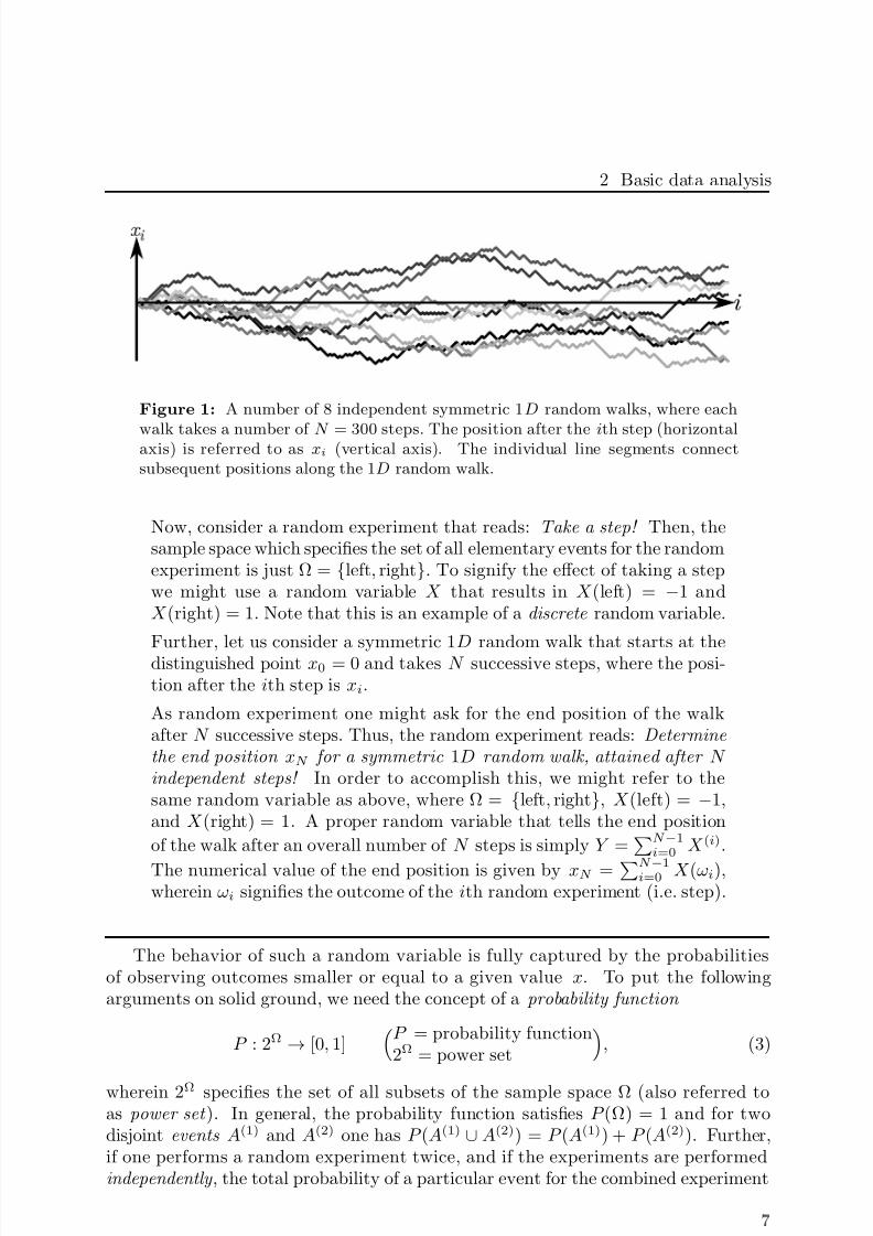
Figure 1: A number of 8 independent symmetric 1D random walks, where each
walk takes a number of N = 300 steps. The position after the ith step (horizontalaxis) is referred to as xi (vertical axis). The individual line segments connectsubsequent positions along the 1D random walk.
Now, consider a random experiment that reads: Take a step! Then, thesample space which specifies the set of all elementary events for the randomexperiment is just Ω = left, right. To signify the effect of taking a stepwe might use a random variable X that results in X (left) = −1 andX (right) = 1. Note that this is an example of a discrete random variable.
Further, let us consider a symmetric 1D random walk that starts at thedistinguished point x0 = 0 and takes N successive steps, where the posi-tion after the ith step is xi.
As random experiment one might ask for the end position of the walkafter N successive steps. Thus, the random experiment reads: Determine the end position xN for a symmetric 1D random walk, attained after N independent steps! In order to accomplish this, we might refer to thesame random variable as above, where Ω = left, right, X (left) = −1,and X (right) = 1. A proper random variable that tells the end position
of the walk after an overall number of N steps is simply Y = N −1i=0 X (i).
The numerical value of the end position is given by xN =
N −1i=0 X (ωi),wherein ωi signifies the outcome of the ith random experiment (i.e. step).
The behavior of such a random variable is fully captured by the probabilitiesof observing outcomes smaller or equal to a given value x. To put the followingarguments on solid ground, we need the concept of a probability function
P : 2Ω → [0, 1]
P = probability function2Ω = power set
, (3)
wherein 2Ω specifies the set of all subsets of the sample space Ω (also referred toas power set ). In general, the probability function satisfies P (Ω) = 1 and for twodisjoint events A(1) and A(2) one has P (A(1) ∪ A(2)) = P (A(1)) + P (A(2)). Further,if one performs a random experiment twice, and if the experiments are performedindependently , the total probability of a particular event for the combined experiment
7/27/2019 Big Data Analysis using Python
http://slidepdf.com/reader/full/big-data-analysis-using-python 8/62
Basic data analysis (Melchert)
is the product of the single-experiment probabilities. I.e., for two events A(1),(2) onehas P (A(1), A(2)) = P (A(1))P (A(2)).
Example: Probability function
For the sample space Ω = left, right, associated to the random variableX considered in the above example on the symmetric 1D random walk, onehas the power set 2Ω = ∅, left, right, left, right. Consequently, theprobability function reads: P (
∅) = 0, P (
left
) = P (
right
) = 0.5, and
P (left, right) = 1. Further, if two successive steps of the symmetric 1Drandom walk are considered, the probability for the (exemplary) combinedoutcome (left, left) reads: P ((left, left)) = P (left)P (left) = 0.25.
By means of the probability function P , the (cumulative ) distribution function F X of a random variable X signifies a function
F X : R → [0, 1], where F X = P (X ≤ x)
F X = distribution functionP = probability function
. (4)
The distribution is non-decreasing, implying that F X(x1) ≤ F X(x2) for x1 < x2, andnormalized, i.e., limx→−∞ F X(x) → 0 and limx→∞ F X(x) → 1. Further, it holds thatP (x0 < X ≤ x1) = F X(x1) − F X(x0).
Considering the result of a sequence of random experiments, it is useful to drawa distinction between different types of data, to be able to choose a proper set of methods and tools for post-processing. Subsequently, we will distinguish betweendiscrete random variables (as, e.g., the 1D random walk used in the above examples)and continuous random variables.
Discrete probability distributions
Besides the concept of the distribution function, an alternative description of a discrete random variable X is possible by means of its associated probability mass function (pmf),
pX : R → [0, 1], where pX(x) = P (X = x) pX = prob. mass functionP = probability function
. (5)
Related to this, note that a discrete random variable can only yield a countablenumber of outcomes (for an elementary step with unit step length in the 1D randomwalk problem these where just
±1) and hence, the pmf is zero almost everywhere.
E.g., the nonzero entries of the pmf related to the random variable X considered inthe context of the symmetric 1D random walk are pX(−1) = pX(1) = 0.5. Finally,the distribution function is related to the pmf via F X(x) =
xi≤x
pX(xi) (where xirefers to those outcomes u for which pX(u) > 0).
7/27/2019 Big Data Analysis using Python
http://slidepdf.com/reader/full/big-data-analysis-using-python 9/62
2 Basic data analysis
0
0.01
0.02
0.03
0.04
0.05
-40 -20 0 20 40
p X ( X = x N )
x N
(a)observedexpected
0
0.25
0.5
0.75
1
-40 -20 0 20 40
F X ( x N )
x N
(b)
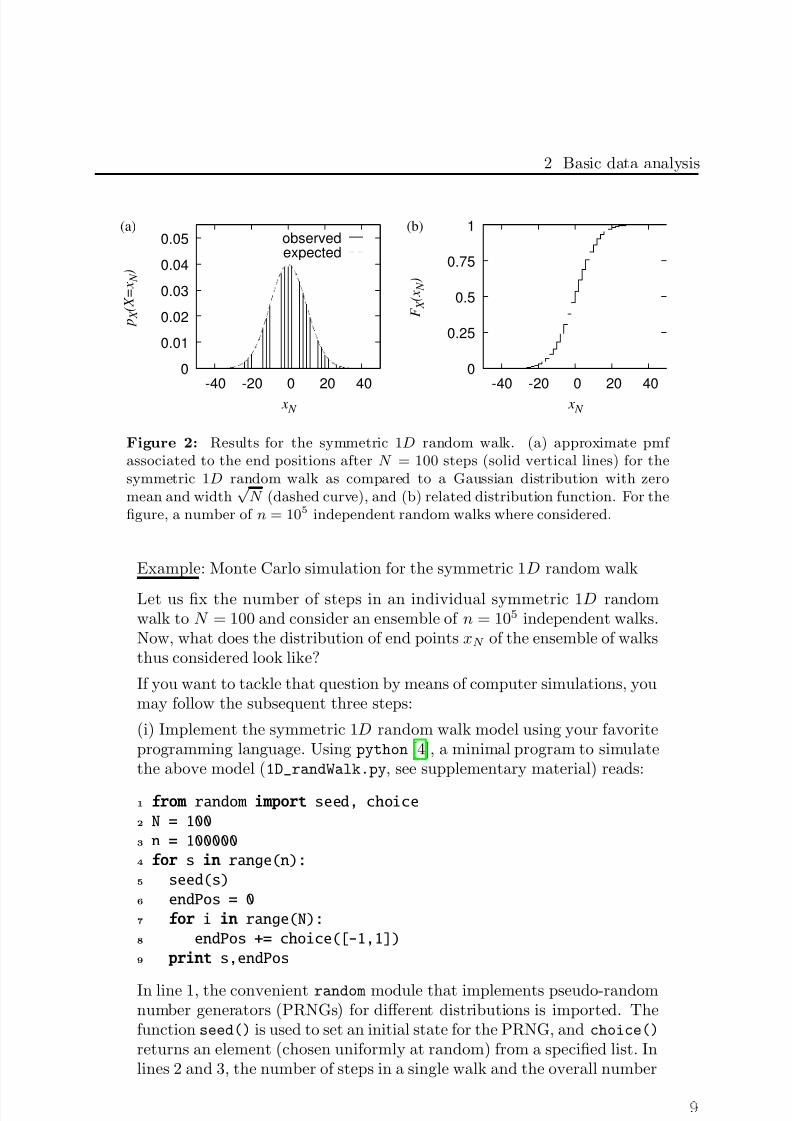
Figure 2: Results for the symmetric 1D random walk. (a) approximate pmf associated to the end positions after N = 100 steps (solid vertical lines) for thesymmetric 1D random walk as compared to a Gaussian distribution with zeromean and width
√ N (dashed curve), and (b) related distribution function. For the
figure, a number of n = 105 independent random walks where considered.
Example: Monte Carlo simulation for the symmetric 1D random walk
Let us fix the number of steps in an individual symmetric 1D randomwalk to N = 100 and consider an ensemble of n = 105 independent walks.Now, what does the distribution of end points xN of the ensemble of walksthus considered look like?
If you want to tackle that question by means of computer simulations, youmay follow the subsequent three steps:
(i) Implement the symmetric 1D random walk model using your favoriteprogramming language. Using python [4], a minimal program to simulatethe above model (1D_randWalk.py, see supplementary material) reads:
1 from random import seed, choice
2 N = 100
3 n = 100000
4 for s in range(n):
5 seed(s)
6 endPos = 0
7 for i in range(N):
8 endPos += choice([-1,1])
9 print s,endPos
In line 1, the convenient random module that implements pseudo-randomnumber generators (PRNGs) for different distributions is imported. Thefunction seed() is used to set an initial state for the PRNG, and choice()
returns an element (chosen uniformly at random) from a specified list. Inlines 2 and 3, the number of steps in a single walk and the overall number
7/27/2019 Big Data Analysis using Python
http://slidepdf.com/reader/full/big-data-analysis-using-python 10/62
Basic data analysis (Melchert)
of independent walks are specified, respectively. In lines 6–7, a singlepath is constructed and the seed as well as the resulting final positionare sent to the standard outstream in line 9. It is a bit tempting toinclude data post-processing directly within the simulation code above.However, from a point of view of data analysis you are more flexible if you store the output of the simulation in an external file. Then it is moreeasy to “revisit” the data, in case you want to (or are asked to) performsome further analyses. Hence, we might invoke the python script on thecommand line and redirect its output as follows
1 > python 1D_randWalk.py > N100_n100000.dat
After the script has terminated successfully, the file N100_n100000.dat
keeps the simulated data available for post-processing at any time.
(ii) An approximate pmf associated to the distribution of end points can beconstructed from the raw data contained in file N100_n100000.dat. Wemight write a small, stand-alone python script that handles that issue.However, from a point of view of code-recycling and modularization it ismore rewarding to collect all “useful” functions, i.e., functions that might
be used again in a different context, in a particular file that serves as somekind of tiny library. If we need a data post-processing script, we can theneasily include the library file and use the functions defined therein. As afurther benefit, the final data analysis scripts will consist of a few linesonly. Here, let us adopt the name MCS2012_lib.py (see supplementarymaterial) for the tiny library file and define two functions as listed below:
1 def fetchData(fName,col=0,dType=int):
2 myList = []
3 file = open(fName,"r" )
4 for line in file:
5 myList.append(dType(line.split()[col]))
6 file.close()
7 return myList
8
9 def getPmf (myList):
10 pMap =
11 nInv = 1./len(myList)
12 for element in myList:
13 if element not in pMap:
14 pMap[element] = 0.
15 pMap[element] += nInv
16 return pMap
Lines 1–7 implement the function fetchData(fName,col=0,dType=int),used to collect data of type dType from column number col (default col-
7/27/2019 Big Data Analysis using Python
http://slidepdf.com/reader/full/big-data-analysis-using-python 11/62
2 Basic data analysis
umn is 0 and default data type is int) from the file named fName. In func-tion getPmf(myList), defined in lines 9–16, the integer numbers (storedin the list myList) are used to approximate the underlying pmf.
So far, we started to build the tiny library. A small data post-processingscript (pmf.py, see supplementary material) that uses the library in orderto construct the pmf from the simulated data reads:
1 import sys
2 from MCS2012_lib import *
3
4 ## parse command line arguments
5 fileName = sys.argv[1]
6 col = int(sys.argv[2])
7
8 ## construct approximate pmf from data
9 rawData = fetchData(fileName,col)
10 pmf = getPmf(rawData)
11
12 ## dump pmf/distrib func. to standard outstream
13 FX = 0.14 for endpos in sorted(pmf):
15 FX += pmf[endpos]
16 print endpos,pmf[endpos],FX
This already illustrates lots of the python functionality that is needed fora decent data post-processing. In line 1, a basic python module, calledsys, is imported. Among other things, it allows to access command lineparameters stored as a list with the default name sys.argv. Note that thefirst entry of the list is reserved for the file name. All “real” command line
parameters start at the list index 1. In line 2, all functions contained in thetiny library MCS2012_lib.py are imported and are available for data post-processing by means of their genuine name (no MCS2012_lib. statementhas to precede a functions name). In lines 14–16, the approximate pmf aswell as the related distribution function are sent to the standard outstream(for a comment on the built-in function sorted(), see paragraph “Basicsorting” in Section 1).
To cut a long story short, the approximate pmf for the end positions of the symmetric 1D random walks stored in the file N100_n100000.dat canbe obtained by calling the script on the command line via
1 > python pmf.py N100_n100000.dat 1 > N100_n100000.pmf
Therein, the digit 1 indicates the column of the supplied file where the endposition of the walks is stored, and the approximate pmf and the relateddistribution function are redirected to the file N100_n100000.pmf.
7/27/2019 Big Data Analysis using Python
http://slidepdf.com/reader/full/big-data-analysis-using-python 12/62
Basic data analysis (Melchert)
(iii) On the basis of analytical theory, one can expect that the enclosingcurve of the pmf is well represented by a Gaussian distribution with mean0 and width
√ N . However, we need to rescale the approximate pmf, i.e.,
the observed probabilities, by a factor of 2 if we want to compare it to theexpected probabilities given by the Gaussian distribution. Therein, thefactor 2 reflects the fact that if we consider walks with an even (or odd)number of steps only, the effective length-scale that characterizes the dis-tance between two neighboring positions is 2. A less handwaving way toarrive at that conclusion is to start with the proper end point distribution
for a symmetric 1D random walk, given by a (discrete) symmetric bino-mial distribution (see Section 2.4), and to approximate it, using Stirlingsexpansion, by a (continuous) distribution. The factor 2 is then immedi-ate. Using the convenient gnuplot plotting program [5], you can visuallyinspect the difference between the observed and expected probabilities bycreating a file, e.g. called endpointDistrib.gp (see supplementary mate-rial), with content:
1 set multiplot
2
3 ## probability mass function
4 set origin 0.,0.
5 set size 0.5,0.65
6 set key samplen 1.
7 set yr [:0.05]; set ytics (0.00,0.02,0.04)
8 set xr [-50:50]
9 set xlabel "x_N" font "Times-Italic"
10 set ylabel "p_X(X=x_N)" font "Times-Italic"
11
12 ## expected probability
13 f (x)=exp(-(x- mu)**2/(2*s*s))/(s*sqrt(2*pi))
14 mu=0; s=10
15
16 p "N100_n100000.pmf" u 1:($2/2) w impulses t "observed" \
17 , f (x) t "expected"
18
19 ## distribution function
20 set origin 0.5,0.
21 set size 0.5,0.65
22 set yr [0:1]; set ytics (0.,0.25,0.5,0.75,1.)
23 set xr [-50:50]
24 set ylabel "F_X(x_N)" font "Times-Italic"
25
26 p "N100_n100000.pmf" u 1:($3) w steps notitle
27
28 unset multiplot
7/27/2019 Big Data Analysis using Python
http://slidepdf.com/reader/full/big-data-analysis-using-python 13/62
2 Basic data analysis
Calling the file via gnuplot -persist endpointDistrib.gp, the outputshould look similar to Fig. 2.
Continuous probability distributions
Given a continuous distribution function F X , the density of a continuous randomvariable X , referred to as probability density function (pdf), reads
pX : R → [0, 1], where pX(x) = dF X(x)dx
pX = prob. density func-tion F X = distributionfunctin
. (6)
The pdf is strictly nonnegative, and, as should be clear from the definition, the prob-ability that X falls within a certain interval, say x → x + ∆x, is given by the integral
of the pdf pX(x) over that interval, i.e. P (x < X ≤ x + ∆x) = x+∆xx pX(u) du.
Since the pdf is normalized, one further has 1 = ∞−∞
pX(u) du.
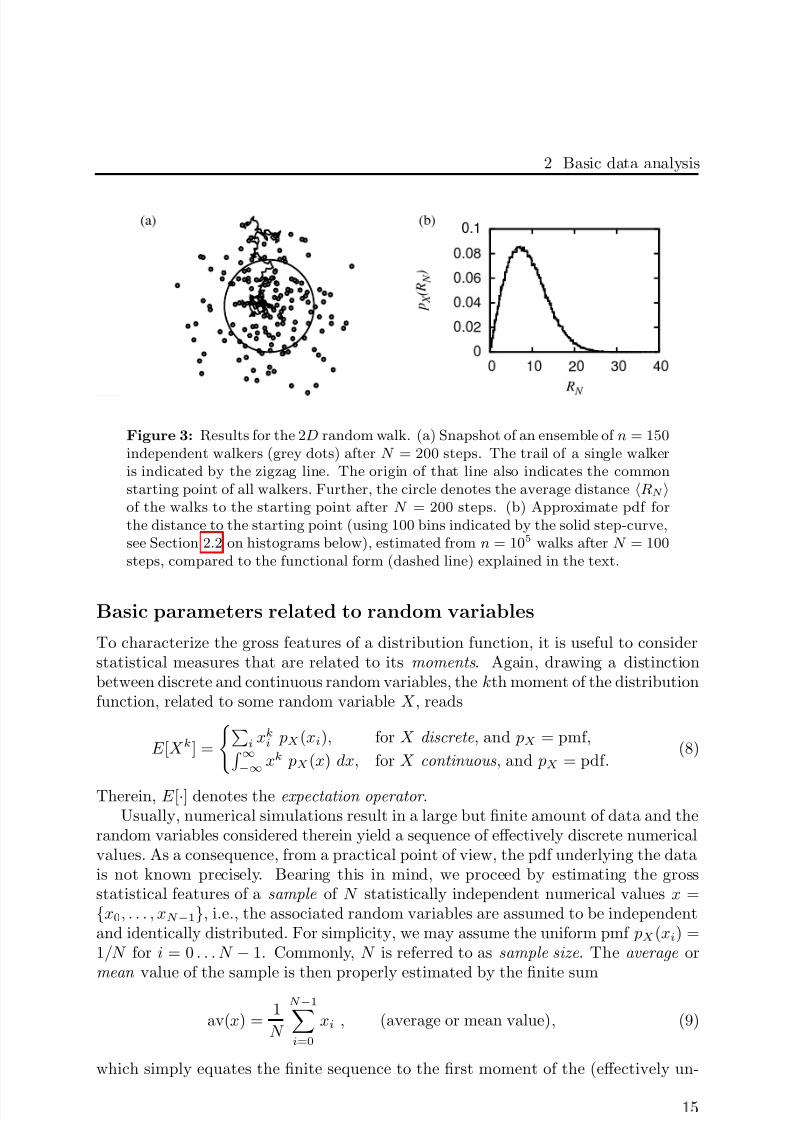
Example: The continuous 2D random walk
The continuous 2D random walk (see Fig. 3) is an example for a randomwalk with fixed step-length (for simplicity assume unit step length), wherethe direction of the consecutive steps is drawn uniformly at random. Ascontinuous random variable X we may choose the distance of the walkto its starting point after a number of N steps, referred to as RN . Toimplement this random walk model, we can recycle the python script forthe 1D random walk, written earlier. A proper code (2d_randWalk.py,see supplementary material) to simulate the model is listed below:
1 from random import seed, random
2
from math import sqrt, cos, sin, pi3
4 N = 100
5 n = 100000
6 for s in range(n):
7 seed(s)
8 x = y = 0.
9 for i in range(N):
10 phi = random()*2*pi
11 x += cos(phi)
12
y += sin(phi)13 print s,sqrt(x*x+y*y)
Therein, in line 10, the direction of the upcoming step is drawn uniformlyat random, and, in lines 11–12, the two independent walk coordinatesare updated. Note that in line 2, the basic mathematical functions and
7/27/2019 Big Data Analysis using Python
http://slidepdf.com/reader/full/big-data-analysis-using-python 14/62
Basic data analysis (Melchert)
constants are imported. Finally, in line 13, the distance RN for a singlewalk is sent to the standard output. Invoking the script on the commandline and redirecting its output to the file 2dRW_N100_n100000.dat, we canfurther obtain an approximation to the underlying pdf by constructing anormalized histogram of the distances RN by means of the script hist.py
(see supplementary material) as follows:
1 > python hist.py 2dRW_N100_n100000.dat 1 100 \
2 > > 2dRW_N100_n100000.pdf
The two latter numbers signify the column of the file, where the relevantdata is stored, and the desired number of bins, respectively. At this point,let us just use the script hist.py as a “black-box” and postpone the dis-cussion of histograms until Section 2.2. After the script has terminatedsuccessfully, the file 2dRW_N100_n100000.pdf contains the normalized his-togram. For values of N large enough, one can expect that RN is properlycharacterized by the Rayleigh distribution
pN (RN ) =RN
σ2
exp
−R2N /(2σ2)
, (7)
where σ2 = (2n)−1n−1
i=0 R2N,i. Therein, the values RN,i, i = 0 . . . n − 1,
comprise the sample of observed distances. In order to compute σ for thesample of observed distances, one could use a cryptic python one-liner.However, it is more readable to accomplish that task in the following way(sigmaRay.py, see supplementary material):
1 import sys, math
2 from MCS2012_lib import fetchData
3
4 rawData = fetchData(sys.argv[1],1,float)
5
6 sum2=0.
7 for val in rawData: sum2+=val*val
8 print "sigma=" ,math.sqrt(sum2/(2.*len(rawData)))
Invoking the script on the command line yields:
1 > python sigmaRay.py 2dRW_N100_n100000.dat
2 sigma= 7.09139394259
Finally, an approximate pdf of the distance to the starting point of thewalkers, i.e., a histogram using 100 bins, as well as the Rayleigh probabilitydistribution function with σ = 7.091 is shown in Fig. 3(b).
7/27/2019 Big Data Analysis using Python
http://slidepdf.com/reader/full/big-data-analysis-using-python 15/62
2 Basic data analysis
Figure 3: Results for the 2D random walk. (a) Snapshot of an ensemble of n = 150independent walkers (grey dots) after N = 200 steps. The trail of a single walkeris indicated by the zigzag line. The origin of that line also indicates the commonstarting point of all walkers. Further, the circle denotes the average distance RN of the walks to the starting point after N = 200 steps. (b) Approximate pdf forthe distance to the starting point (using 100 bins indicated by the solid step-curve,see Section 2.2 on histograms below), estimated from n = 105 walks after N = 100steps, compared to the functional form (dashed line) explained in the text.
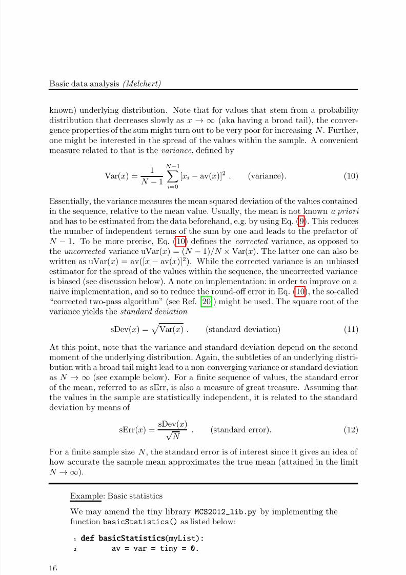
Basic parameters related to random variables
To characterize the gross features of a distribution function, it is useful to considerstatistical measures that are related to its moments . Again, drawing a distinctionbetween discrete and continuous random variables, the kth moment of the distributionfunction, related to some random variable X , reads
E [X k] =
i xki pX(xi), for X discrete , and pX = pmf,
∞
−∞ xk pX(x) dx, for X continuous , and pX = pdf.(8)
Therein, E [·] denotes the expectation operator .Usually, numerical simulations result in a large but finite amount of data and the
random variables considered therein yield a sequence of effectively discrete numericalvalues. As a consequence, from a practical point of view, the pdf underlying the datais not known precisely. Bearing this in mind, we proceed by estimating the grossstatistical features of a sample of N statistically independent numerical values x =x0, . . . , xN −1, i.e., the associated random variables are assumed to be independentand identically distributed. For simplicity, we may assume the uniform pmf pX(xi) =1/N for i = 0 . . . N − 1. Commonly, N is referred to as sample size . The average ormean value of the sample is then properly estimated by the finite sum
av(x) =1
N
N −1i=0
xi , (average or mean value), (9)
which simply equates the finite sequence to the first moment of the (effectively un-
7/27/2019 Big Data Analysis using Python
http://slidepdf.com/reader/full/big-data-analysis-using-python 16/62
Basic data analysis (Melchert)
known) underlying distribution. Note that for values that stem from a probabilitydistribution that decreases slowly as x → ∞ (aka having a broad tail), the conver-gence properties of the sum might turn out to be very poor for increasing N . Further,one might be interested in the spread of the values within the sample. A convenientmeasure related to that is the variance , defined by
Var(x) =1
N − 1
N −1i=0
[xi − av(x)]2 . (variance). (10)
Essentially, the variance measures the mean squared deviation of the values containedin the sequence, relative to the mean value. Usually, the mean is not known a priori and has to be estimated from the data beforehand, e.g. by using Eq. (9). This reducesthe number of independent terms of the sum by one and leads to the prefactor of N − 1. To be more precise, Eq. (10) defines the corrected variance, as opposed tothe uncorrected variance uVar(x) = (N − 1)/N × Var(x). The latter one can also bewritten as uVar(x) = av([x − av(x)]2). While the corrected variance is an unbiasedestimator for the spread of the values within the sequence, the uncorrected varianceis biased (see discussion below). A note on implementation: in order to improve on anaive implementation, and so to reduce the round-off error in Eq. (10), the so-called
“corrected two-pass algorithm” (see Ref. [20]) might be used. The square root of thevariance yields the standard deviation
sDev(x) =
Var(x) . (standard deviation) (11)
At this point, note that the variance and standard deviation depend on the secondmoment of the underlying distribution. Again, the subtleties of an underlying distri-bution with a broad tail might lead to a non-converging variance or standard deviationas N → ∞ (see example below). For a finite sequence of values, the standard errorof the mean, referred to as sErr, is also a measure of great treasure. Assuming thatthe values in the sample are statistically independent, it is related to the standarddeviation by means of
sErr(x) =sDev(x)√
N . (standard error). (12)
For a finite sample size N , the standard error is of interest since it gives an idea of how accurate the sample mean approximates the true mean (attained in the limitN → ∞).
Example: Basic statistics
We may amend the tiny library MCS2012_lib.py by implementing thefunction basicStatistics() as listed below:
1 def basicStatistics(myList):
2 av = var = tiny = 0.
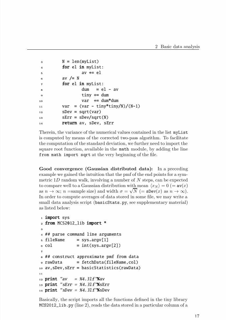
7/27/2019 Big Data Analysis using Python
http://slidepdf.com/reader/full/big-data-analysis-using-python 17/62
2 Basic data analysis
3 N = len(myList)
4 for el in myList:
5 av += el
6 av /= N
7 for el in myList:
8 dum = el - av
9 tiny += dum
10 var += dum *dum
11 var = (var - tiny*tiny/N)/(N-1)
12 sDev = sqrt(var)13 sErr = sDev/sqrt(N)
14 return av, sDev, sErr
Therein, the variance of the numerical values contained in the list myList
is computed by means of the corrected two-pass algorithm. To facilitatethe computation of the standard deviation, we further need to import thesquare root function, available in the math module, by adding the linefrom math import sqrt at the very beginning of the file.
Good convergence (Gaussian distributed data): In a precedingexample we gained the intuition that the pmf of the end points for a sym-metric 1D random walk, involving a number of N steps, can be expectedto compare well to a Gaussian distribution with mean xN = 0 (= av(x)as n → ∞; n =sample size) and width σ =
√ N (= sDev(x) as n → ∞).
In order to compute averages of data stored in some file, we may write asmall data analysis script (basicStats.py, see supplementary material)as listed below:
1 import sys
2
from MCS2012_lib import *3
4 ## parse command line arguments
5 fileName = sys.argv[1]
6 col = int(sys.argv[2])
7
8 ## construct approximate pmf from data
9 rawData = fetchData(fileName,col)
10 av,sDev,sErr = basicStatistics(rawData)
11
12
print "av = %4.3lf " % av13 print "sErr = %4.3lf" % sErr
14 print "sDev = %4.3lf" % sDev
Basically, the script imports all the functions defined in the tiny libraryMCS2012_lib.py (line 2), reads the data stored in a particular column of a
7/27/2019 Big Data Analysis using Python
http://slidepdf.com/reader/full/big-data-analysis-using-python 18/62
Basic data analysis (Melchert)
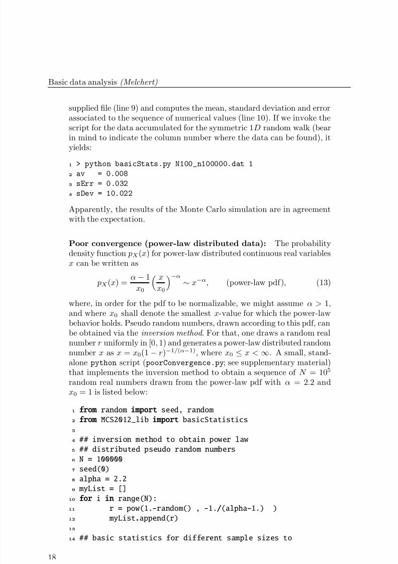
supplied file (line 9) and computes the mean, standard deviation and errorassociated to the sequence of numerical values (line 10). If we invoke thescript for the data accumulated for the symmetric 1D random walk (bearin mind to indicate the column number where the data can be found), ityields:
1 > python basicStats.py N100_n100000.dat 1
2 av = 0.008
3 sErr = 0.032
4 sDev = 10.022
Apparently, the results of the Monte Carlo simulation are in agreementwith the expectation.
Poor convergence (power-law distributed data): The probabilitydensity function pX(x) for power-law distributed continuous real variablesx can be written as
pX(x) =α − 1
x0 x
x0−α
∼ x−α, (power-law pdf), (13)
where, in order for the pdf to be normalizable, we might assume α > 1,and where x0 shall denote the smallest x-value for which the power-lawbehavior holds. Pseudo random numbers, drawn according to this pdf, canbe obtained via the inversion method . For that, one draws a random realnumber r uniformly in [0, 1) and generates a power-law distributed randomnumber x as x = x0(1 − r)−1/(α−1), where x0 ≤ x < ∞. A small, stand-alone python script (poorConvergence.py; see supplementary material)that implements the inversion method to obtain a sequence of N = 105
random real numbers drawn from the power-law pdf with α = 2.2 and
x0 = 1 is listed below:1 from random import seed, random
2 from MCS2012_lib import basicStatistics
3
4 ## inversion method to obtain power law
5 ## distributed pseudo random numbers
6 N = 100000
7 seed(0)
8 alpha = 2.2
9 myList = []
10 for i in range(N):
11 r = pow(1.-random() , -1./(alpha-1.) )
12 myList.append(r)
13
14 ## basic statistics for different sample sizes to
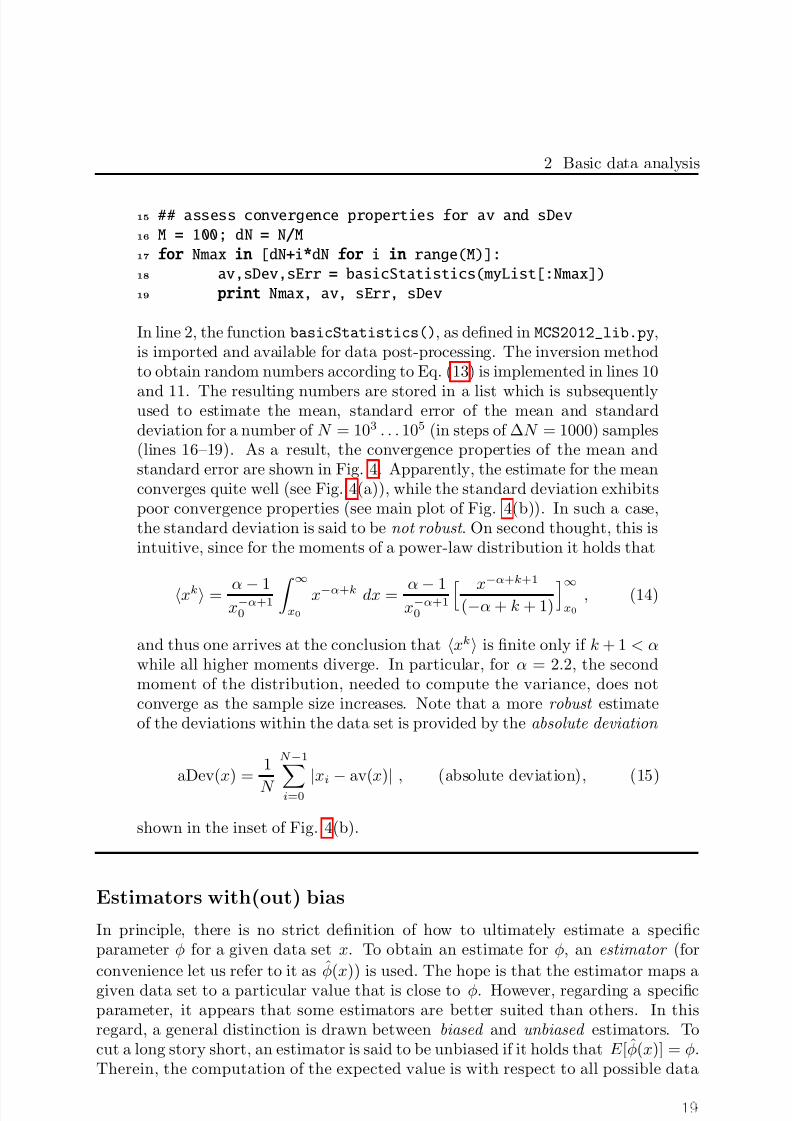
7/27/2019 Big Data Analysis using Python
http://slidepdf.com/reader/full/big-data-analysis-using-python 19/62
2 Basic data analysis
15 ## assess convergence properties for av and sDev
16 M = 100; dN = N/M
17 for Nmax in [dN+i*dN for i in range(M)]:
18 av,sDev,sErr = basicStatistics(myList[:Nmax])
19 print Nmax, av, sErr, sDev
In line 2, the function basicStatistics(), as defined in MCS2012_lib.py,is imported and available for data post-processing. The inversion methodto obtain random numbers according to Eq. (13) is implemented in lines 10
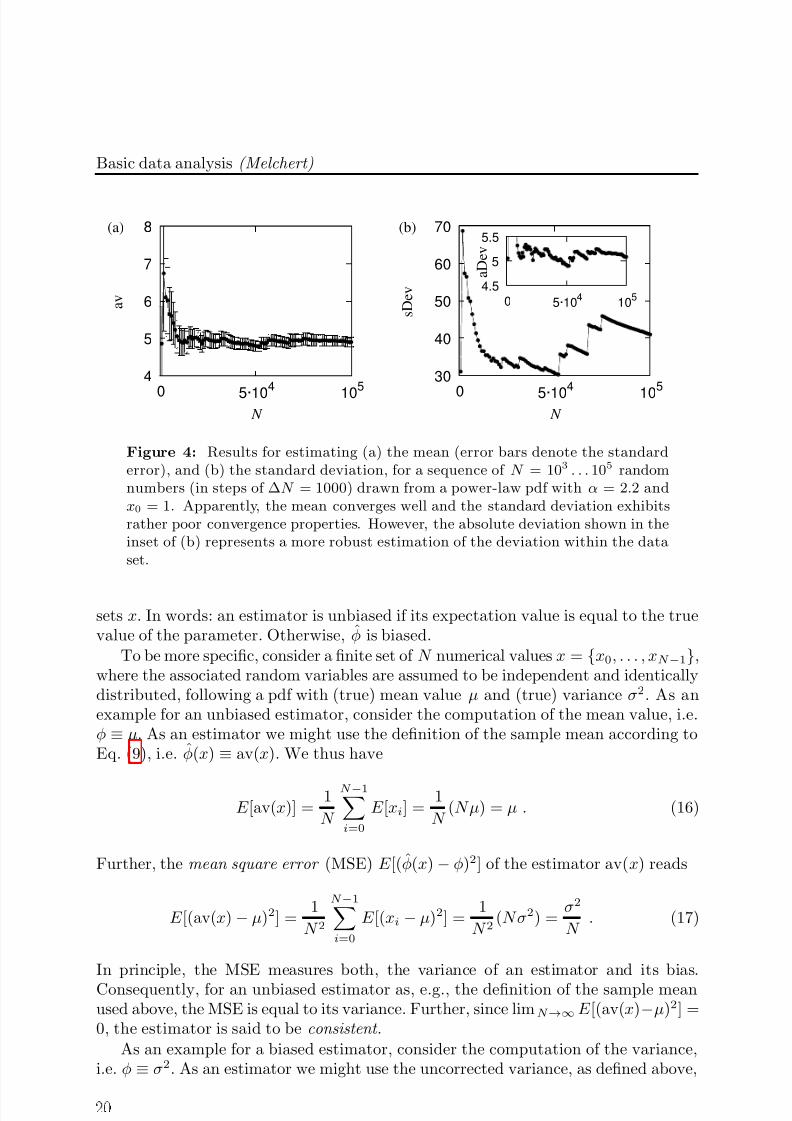
and 11. The resulting numbers are stored in a list which is subsequentlyused to estimate the mean, standard error of the mean and standarddeviation for a number of N = 103 . . . 105 (in steps of ∆N = 1000) samples(lines 16–19). As a result, the convergence properties of the mean andstandard error are shown in Fig. 4. Apparently, the estimate for the meanconverges quite well (see Fig. 4(a)), while the standard deviation exhibitspoor convergence properties (see main plot of Fig. 4(b)). In such a case,the standard deviation is said to be not robust . On second thought, this isintuitive, since for the moments of a power-law distribution it holds that
xk = α − 1x−α+10
∞x0
x−α+k dx = α − 1x−α+10
x−α+k+1
(−α + k + 1)∞x0
, (14)
and thus one arrives at the conclusion that xk is finite only if k + 1 < αwhile all higher moments diverge. In particular, for α = 2.2, the secondmoment of the distribution, needed to compute the variance, does notconverge as the sample size increases. Note that a more robust estimateof the deviations within the data set is provided by the absolute deviation
aDev(x) =1
N
N −1
i=0 |
xi−
av(x)|
, (absolute deviation), (15)
shown in the inset of Fig. 4(b).
Estimators with(out) bias
In principle, there is no strict definition of how to ultimately estimate a specificparameter φ for a given data set x. To obtain an estimate for φ, an estimator (for
convenience let us refer to it as φ(x)) is used. The hope is that the estimator maps a
given data set to a particular value that is close to φ. However, regarding a specificparameter, it appears that some estimators are better suited than others. In thisregard, a general distinction is drawn between biased and unbiased estimators. Tocut a long story short, an estimator is said to be unbiased if it holds that E [φ(x)] = φ.Therein, the computation of the expected value is with respect to all possible data
7/27/2019 Big Data Analysis using Python
http://slidepdf.com/reader/full/big-data-analysis-using-python 20/62
Basic data analysis (Melchert)
4
5
6
7
8
0 5·10
4
10
5
a v
N
(a)
30
40
50
60
70
0 5·10
4
10
5
s D e v
N
(b)
4.5
5
5.5
0 5·104
105
a D e v
Figure 4: Results for estimating (a) the mean (error bars denote the standarderror), and (b) the standard deviation, for a sequence of N = 103 . . . 105 randomnumbers (in steps of ∆N = 1000) drawn from a power-law pdf with α = 2.2 andx0 = 1. Apparently, the mean converges well and the standard deviation exhibitsrather poor convergence properties. However, the absolute deviation shown in theinset of (b) represents a more robust estimation of the deviation within the dataset.
sets x. In words: an estimator is unbiased if its expectation value is equal to the truevalue of the parameter. Otherwise, φ is biased.
To be more specific, consider a finite set of N numerical values x = x0, . . . , xN −1,where the associated random variables are assumed to be independent and identicallydistributed, following a pdf with (true) mean value µ and (true) variance σ2. As anexample for an unbiased estimator, consider the computation of the mean value, i.e.φ ≡ µ. As an estimator we might use the definition of the sample mean according toEq. (9), i.e. φ(x) ≡ av(x). We thus have
E [av(x)] =1
N
N −1i=0
E [xi] =1
N (N µ) = µ . (16)
Further, the mean square error (MSE) E [(φ(x) − φ)2] of the estimator av(x) reads
E [(av(x) − µ)2] =1
N 2
N −1i=0
E [(xi − µ)2] =1
N 2(N σ2) =
σ2
N . (17)
In principle, the MSE measures both, the variance of an estimator and its bias.
Consequently, for an unbiased estimator as, e.g., the definition of the sample meanused above, the MSE is equal to its variance. Further, since limN →∞ E [(av(x)−µ)2] =0, the estimator is said to be consistent .
As an example for a biased estimator, consider the computation of the variance,i.e. φ ≡ σ2. As an estimator we might use the uncorrected variance, as defined above,
7/27/2019 Big Data Analysis using Python
http://slidepdf.com/reader/full/big-data-analysis-using-python 21/62
2 Basic data analysis
to find
E [uVar(x)] =1
N
N −1i=0
E [(xi − µ)2] − E [(av(x) − µ)2] =N − 1
N σ2 . (18)
Since here it holds that E [uVar(x)] = σ2, the uncorrected variance is biased. Notethat the (corrected) variance, defined in Eq. (10), provides an unbiased estimate of σ2.Finally, note that the question whether bias arises is solely related to the estimator,not the estimate (obtained from a particular data set).
2.2 Histograms: binning and graphical representation of data
In the preceding section, we have already used histograms as a tool to construct ap-proximate distribution functions from a finite set of data. Now, to provide a moreprecise definition of a histogram , consider a data set x ≡ xiN −1i=0 that stems fromrepeated measurements of a continuous random variable X during a random experi-ment. To get a gross idea of the properties of the underlying continuous distributionfunction, and to allow for a graphical representation of the respective data, e.g., forthe purpose of communicating results to the scientific community, a histogram of theobserved data is of great use.
The idea is simply to accumulate the elements of the data set x in a finite numberof, say, n distinct intervals (or classes) C i = [ci, ci+1), i = 0 . . . n−1, called bins , wherethe ci specify the interval boundaries. The frequency density hi (i.e., the relativefrequency per unit-interval) associated with the ith bin can easily be obtained ashi = ni/(N ∆ci), where ni specifies the number of elements that fall into bin C i, and∆ci = ci+1 − ci is the respective bin width. The resulting set H of tuples (C i, hi), i.e.
H = (C i, hi)n−1i=0 ,
C i = [ci, ci+1), i.e. the ith binhi = frequency density
, (19)
specifies the histogram and give a discrete approximation to the pdf underlying the
random variable. Note that if one considers a finite sample size N , it is only possibleto construct an approximate pdf. However, as the sample size increases one can beconfident to approximate the true pdf quite well. All the values that fall within acertain bin C i are further represented by a particular value xi ∈ C i. Often, xi ischosen as the center of the bin. Also note that, in order to properly represent theobserved data, it might be useful to choose different widths ∆ci = ci+1 − ci for thedifferent bins bi. As an example, one may decide to go for linear or logarithmic binning , detailed below.
Linear binning
Considering linear binning , the whole range of data [xmin, xmax) is collected using nbins of equal width ∆c = (xmax − xmin)/n. Therein, a particular bin C i accumulatesall elements in the interval [ci, ci+1), where the interval bounds are given by
ci = xmin + i∆c , for i = 0 . . . n . (20)
7/27/2019 Big Data Analysis using Python
http://slidepdf.com/reader/full/big-data-analysis-using-python 22/62
Basic data analysis (Melchert)
During the binning procedure, a particular element belongs to bin C i, where theinteger identifier of the bin is given by i = x/∆c.
Logarithmic binning
Considering logarithmic binning , the whole range of data [xmin, xmax) is collectedwithin n bins that have equal width on a logarithmic scale, i.e., log(ci+1) = log(ci) +∆c where ∆c = log(xmax/xmin)/n. In case of logarithmic binning, a particular binC i accumulates all elements in the interval [ci, ci+1), where the interval bounds are
consequently given by
ci = c0 × expi∆c , for i = 0 . . . n . (21)
During the histogram build-up, a particular element belongs to bin C i, where i =log(x/xmin)/∆c. Note that on a linear scale, the width of the bins increases expo-nentially, i.e. ∆ci = ci × (exp∆c − 1) ∝ ci. Such a binning is especially well suitedto represent power-law distributed data, see the example below.
A general drawback of any binning procedure is that many data in a given range[ci, ci+1) are represented by only a single representative xi of that interval. As a
consequence, data binning always comes to the expense of information loss.
Example: Data binning
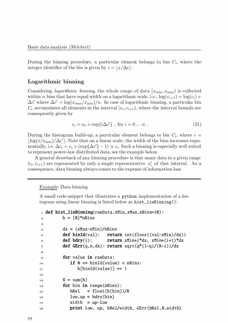
A small code-snippet that illustrates a python implementation of a his-togram using linear binning is listed below as hist_linBinning():
1 def hist_linBinning(rawData,xMin,xMax,nBins=10):
2 h = [0]*nBins
3
4 dx = (xMax-xMin)/nBins
5 def binId(val): return int(floor((val-xMin)/dx))
6 def bdry(i): return xMin+i*dx, xMin+(i+1)*dx
7 def GErr(q,n,dx): return sqrt(q*(1-q)/(N-1))/dx
8
9 for value in rawData:
10 if 0 <= binId(value) < nBins:
11 h[binId(value)] += 1
12
13 N = sum(h)
14 for bin in range(nBins):
15 hRel = float(h[bin])/N
16 low,up = bdry(bin)
17 width = up-low
18 print low, up, hRel/width, GErr(hRel,N,width)
7/27/2019 Big Data Analysis using Python
http://slidepdf.com/reader/full/big-data-analysis-using-python 23/62
2 Basic data analysis
The first argument in the function call, see line 1 of the code listing,indicates a list of the raw data, followed by the minimal and maximalvariable value that should be considered during the binning procedure.The last argument in the function call specifies the number of bins thatshall be used therein (the default value is set to 10). Based on the supplieddata range and number of bins, the uniform bin width is computed in line4. Note that within the function hist_linBinning(), 3 more functionsare defined. Those facilitate the calculation of the integer bin id thatcorresponds to an element of the raw data (line 5), the lower and upper
boundaries of a bin (line 6), and the Gaussian error bar for the respectivedata point (line 7). In lines 9–11, the binning procedure is kicked off. Sincethe upper bin boundary is exclusive, bear in mind that the numerical valuexMax is identified with the bin index nBins+1. As a consequence it willnot be considered during the histogram build-up. Finally, in lines 13–18the resulting normalized bin entries and their associated errors are sent tothe standard out-stream. The function is written in a quite general form,so that in order to implement a different kind of binning procedure onlythe definitions in lines 4–7 have to be modified. As regards this, for a moreversatile variant that offers linear or logarithmic binning of the data, see
the function hist in the tiny library MCS2012_lib.py.
Binning of the data obtained for the 2D random walk: The ap-proximate pdf of the average distance to the starting point for 105 inde-pendent 100-step 2D random walks, see Fig. 3, was obtained by a linearbinning procedure using the function hist_linBinning() outlined above.For that task, the small script hist.py listed below (see supplementarymaterial) was used:
1 import sys
2 from MCS2012_lib import fetchData, hist_linBinning3
4 fName = sys.argv[1]
5 col = int(sys.argv[2])
6 nBins = int(sys.argv[3])
7 myData = fetchData(fName,col,float)
8 hist_linBinning(myData,min(myData),max(myData),nBins)
In principle, the Gaussian error bars are adequate for that data. However,for a clearer presentation of the results, the error bars are not shown in
Fig. 3(b).
Binning of power-law distributed data: To illustrate the pros andcons of the binning types introduced above, consider a data set consistingof N = 106 random numbers drawn from the power-law pdf, Eq. (13), with
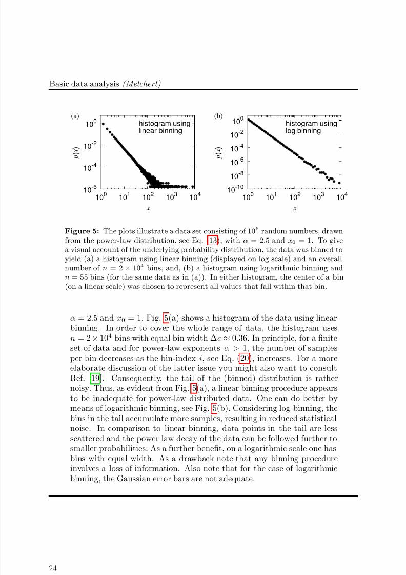
7/27/2019 Big Data Analysis using Python
http://slidepdf.com/reader/full/big-data-analysis-using-python 24/62
Basic data analysis (Melchert)
10-6
10-4
10-2
100
100
101
102
103
104
p ( x )
x
(a)histogram usinglinear binning
10-10
10-8
10-6
10-4
10-2
100
100
101
102
103
104
p ( x )
x
(b)histogram usinglog binning
Figure 5: The plots illustrate a data set consisting of 106 random numbers, drawnfrom the power-law distribution, see Eq. (13), with α = 2.5 and x0 = 1. To givea visual account of the underlying probability distribution, the data was binned toyield (a) a histogram using linear binning (displayed on log scale) and an overallnumber of n = 2 × 10⁴ bins, and, (b) a histogram using logarithmic binning andn = 55 bins (for the same data as in (a)). In either histogram, the center of a bin(on a linear scale) was chosen to represent all values that fall within that bin.
α = 2.5 and x0 = 1. Fig. 5(a) shows a histogram of the data using linearbinning. In order to cover the whole range of data, the histogram usesn = 2 × 10⁴ bins with equal bin width ∆c ≈ 0.36. In principle, for a finiteset of data and for power-law exponents α > 1, the number of samplesper bin decreases as the bin-index i, see Eq. (20), increases. For a moreelaborate discussion of the latter issue you might also want to consultRef. [19]. Consequently, the tail of the (binned) distribution is rathernoisy. Thus, as evident from Fig. 5(a), a linear binning procedure appearsto be inadequate for power-law distributed data. One can do better bymeans of logarithmic binning, see Fig. 5(b). Considering log-binning, thebins in the tail accumulate more samples, resulting in reduced statisticalnoise. In comparison to linear binning, data points in the tail are lessscattered and the power law decay of the data can be followed further tosmaller probabilities. As a further benefit, on a logarithmic scale one hasbins with equal width. As a drawback note that any binning procedureinvolves a loss of information. Also note that for the case of logarithmicbinning, the Gaussian error bars are not adequate.
7/27/2019 Big Data Analysis using Python
http://slidepdf.com/reader/full/big-data-analysis-using-python 25/62
2 Basic data analysis
2.3 Bootstrap resampling: the unbiased way to estimate er-rors
In a previous section, we discussed different parameters that may serve to characterizethe statistical properties of a finite set of data. Amongst others, we discussed estima-tors for the sample mean and standard deviation. While there was a straight forwardestimator for the standard error of the sample mean, there was no such measure forthe standard deviation. As a remedy, the current section illustrates a method thatproves to be highly valuable when it comes to the issue of estimating errors related to
quite a lot of observables (for some more details you might want to consult chapter15.6 of Ref. [20]), in an unbiased way. To get an idea about the subtleties of themethod, picture the following situation: you perform a sequence of random experi-ments for a given model system and generate a sample x, consisting of N statisticallyindependent numbers.
Your aim is to measure some quantity q , e.g. some function q ≡ f (x), that char-acterizes the simulated data. At this point, bear in mind that this does not yieldthe true quantity q that characterizes the model under consideration. Instead, thenumerical value of q (very likely) differs from the latter value to some extent. To pro-vide an error estimate that quantifies how good the observed value q approximatesthe true value q , the bootstrap method utilizes a Monte Carlo simulation. This can bedecomposed into the following two-step procedure: Given a data set x that consistsof N numerical values, where the corresponding random variables are assumed to beindependent and identically distributed:
(i) generate a number of M auxiliary bootstrap data sets x(k), k = 0 . . . M − 1by means of a resampling procedure. To obtain one such data set, draw N data points (with replacement) from the original set x. During the constructionprocedure of a particular data set, some of the elements contained in x will bechosen multiple times, while others won’t appear at all;
(ii) measure the observable of interest for each auxiliary data set, to yield the set of estimates q = q kM −1
k=0 . Estimate the value of the desired observable using theoriginal data set and compute the corresponding error as the standard deviation
sDev(q ) = 1
M − 1
M −1k=0
[q k − av(q )]21/2
(bootstrap error estimate) (22)
of the M resampled (auxiliary) bootstrap data sets.
The finite sample x only allows to get a coarse-grained glimpse on the probabilitydistribution underlying the data. In principle, the latter one is not known. Now,
the basic assumption on which the bootstrap method relies is that the values q k(as obtained from the auxiliary data sets x(k)) are distributed around the value q (obtained from x) in a way similar to how further estimates of the observable obtainedfrom further independent simulations are distributed around q . From a practicalpoint of view, the procedure outlined above works quite well.
7/27/2019 Big Data Analysis using Python
http://slidepdf.com/reader/full/big-data-analysis-using-python 26/62
Basic data analysis (Melchert)
Example: Error estimation via bootstrap resampling
The code snippet below lists a python implementation of the bootstrapmethod outlined above. It is most convenient to amend the tiny li-brary by the function bootstrap(). Note that it makes reference tobasicStatistics(), already defined in MCS2012_lib.py.
1 def bootstrap(myData,estimFunc,M=128):
2 N = len(myData)
3 h = [0.0]*M
4 bootSamp = [0.0]*N5 for sample in range(M):
6 for val in range(N):
7 bootSamp[val] = myData[randint(0,N-1)]
8 h[sample] = estimFunc(bootSamp)
9 origEstim = estimFunc(myData)
10 resError = basicStatistics(h)[1]
11 return origEstim,resError
In lines 5–8, a number of M auxiliary bootstrap data sets are obtained
(the default number of auxiliary data sets is set to M = 128, see func-tion call in line 1). In line 9, the desired quantity, implemented by thefunction estimFunc, is computed for the original data set. Finally, thecorresponding error is found as the standard deviation of the M estimatesof estimFunc for the auxiliary data sets in line 10. Note that the func-tion bootstrap() needs integer random numbers, uniformly drawn in theinterval 0 . . . N − 1, in order to generate the auxiliary data sets. For thispurpose the line from random import randint must be included at thebeginning of the file MCS2012_lib.py.
As an example we may write the following small script that computes
the mean and standard deviation, along with an error for those quantitiescomputed using the bootstrap method, for the data accumulated earlierfor the symmetric 1D random walk (bootstrap.py, see supplementarymaterial).
1 import sys
2 from MCS2012_lib import *
3
4 fileName = sys.argv[1]
5 M = int(sys.argv[2])
6 rawData = fetchData(fileName,1)
7
8 def mean(array): return basicStatistics(array)[0]
9 def sDev(array): return basicStatistics(array)[1]
10
11 print "# estimFunc: q +/- dq"
7/27/2019 Big Data Analysis using Python
http://slidepdf.com/reader/full/big-data-analysis-using-python 27/62
2 Basic data analysis
12 print "mean: %5.3lf +/- %4.3lf " % bootstrap(rawData,mean,M)
13 print "sDev: %5.3lf +/- %4.3lf " % bootstrap(rawData,sDev,M)
Note that the statement from MCS2012_lib import * imports all func-tions from the indicated file and makes them available for data post-processing. Invoking the script on the command line via
1 > python bootstrap.py N100_n100000.dat 1024
where the latter number specifies the desired number of bootstrap samples,the bootstrap method yields the results:
1 # estimFunc: q +/- dq
2 mean: 0.008 +/- 0.032
3 sDev: 10.022 +/- 0.022
For the sample mean, the bootstrap error is in good agreement with thestandard error sErr(x) = 0.032 estimated in the “basic statistics” example(as it should be). Regarding the bootstrap error for the standard devia-tion, the result is in agreement with the expectation σ = 10 (for a number
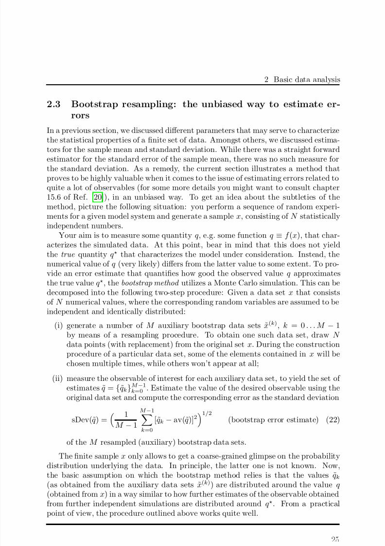
of 100 steps in an individual walk). In Fig. 6, the resulting distributionof the resampled estimates for the mean value (see Fig. 6(a)) and stan-dard error (see Fig. 6(b)) are illustrated. For comparison, if we reducethe number of bootstrap samples to M = 24 we obtain the two bootstraperrors 0.033 and 0.024 for the mean and standard error, respectively.
2.4 The chi-square test: observed vs. expected
The chi-square (χ
2
) goodness-of-fit test is commonly used to check whether the ap-proximate pdf obtained from a set of sampled data appears to be equivalent to atheoretical density function. Here, “equivalent” is meant in the sense of “the ob-served frequencies, as obtained from the data set, are consistent with the expectedfrequencies, as obtained from assuming the theoretical distribution function”. Moreprecisely, assume that you obtained a set (C i, ni)n−1i=0 of binned data, summarizingan original data set of N uncorrelated numerical values, where C i = [ci, ci+1) signifiesthe ith bin with boundaries ci and ci+1, and ni is the number of observed events thatfall within that bin. With reference to Section 2.2, the set of binned data is referred toas frequency histogram . Further, assume you already have a (more or less educated)guess about the expected limiting distribution function underlying the data, whichwe call f (x) in the following. Considering this expected limiting function, the numberof expected events in the ith bin can be estimated as
ei = N × ci+1ci
f (x) dx (expected frequencies). (23)
7/27/2019 Big Data Analysis using Python
http://slidepdf.com/reader/full/big-data-analysis-using-python 28/62
Basic data analysis (Melchert)
0
4
8
12
16
-0.1 -0.05 0 0.05 0.1
p ( a v )
av
(a)
0
5
10
15
20
9.95 10 10.05 10.1
p ( s D e v )
sDev
(b)
Figure 6: Result of the bootstrap resampling procedure (M = 1024 auxiliarydata sets) for the data characterizing the end point distribution for the symmetric1D random walk. (a) Approximate pdf (histogram using 18 bins) of the resampledaverage value. The non-filled square marks the mean value and the associated errorbar indicates the standard error as obtained in the example on “basic statistics”in Section 2.1. (b) Approximate pdf (histogram using 18 bins) of the resampledstandard deviation. The estimate of both quantities, as obtained from the originaldata set, is indicated by a solid vertical line, while the bootstrap error bounds are
shown by dashed vertical lines.
To address the question whether the observed data might possibly be drawn fromf (x), the chi-square test compares the number of observed events in a given bin tothe number of expected events in that bin by means of the expression
χ2 =
n−1i=0
(ni − ei)2
ei(chi-square test). (24)
A further quantity that is important in relation to that test is the number of degrees of freedom, termed dof. Usually it is equal to the number of bins less 1,reflecting the fact that the sum of the expected events has been re-normalized tomatch the sample size of the original data set, i.e.
i ei = N . However, if the function
f (x) involves additional free parameters that have to be determined from the originaldata in order to properly represent the expected limiting distribution function, eachof these free parameters decreases the number of degrees of freedom by one. Now, thewisdom behind the chi-square test is that for χ2 ≈ dof, one can consider the observeddata as being consistent with the expected limiting distribution function. If it holdsthat χ2 dof, then the discrepancy between both is significant. Besides listing thevalues of χ2 and dof, a more convenient way to state the result of the chi-square
test is to report the reduced chi-square , i.e. chi-square per dof, χ2 = χ2/dof. It isindependent of the number of degrees of freedom and the observed data is consistentwith the expected distribution function if χ2 ≈ 1.
For an account of more strict criteria that allow to assess the “quality” of the chi-square test and what to pay attention to if one attempts to compare two sets of binned
7/27/2019 Big Data Analysis using Python
http://slidepdf.com/reader/full/big-data-analysis-using-python 29/62
2 Basic data analysis
data that summarize data sets with possibly different sample sizes, see Refs. [17, 20].Let us leave it at that. As a final note, notice that the chi-square test cannot be usedto prove that the observed data is drawn from an expected distribution function, itmerely reports whether the observed data is consistent with it.
Example: Chi-square test
The code snippet below lists a python implementation of the chi-squaretest outlined above. It is most convenient to amend MCS2012_lib.py by
the function definition1 def chiSquare(obsFreq,expFreq,nConstr):
2 nBins = len(obsFreq)
3 chi2 = 0.0
4 for bin in range(nBins):
5 dum = obsFreq[bin]-expFreq[bin]
6 chi2 += dum *dum /expFreq[bin]
7 dof = nBins-nConstr
8 return dof,chi2
A word of caution: it is a good advise to not trust a chi-square test forwhich some of the observed frequencies are less than, say, 4 (see Ref. [12]).For such small frequencies, the statistical noise is simply too large andthe respective terms might lead to an exploding value of χ2. As a remedyone can merge a couple of adjacent bins to form a “super-bin” containingmore than just 4 events.
For an illustrational purpose we might perform a chi-square test for theapproximate pmf of the end positions of the symmetric 1D random walks,constructed earlier in Section 2.1. In this regard, let (xi, ni)n−1i=0 bethe binned set of data, summarizing an original data set (for a discrete
random variable) with sample size M . Therein, ni denotes the number of observed events that correspond to the value xi. For the data at hand, theexpected frequencies ei are simply proportional to the symmetric binomialdistribution with variance N/4 (where N is the number of steps in a singlewalk) at xi. To be more precise, we have
ei = M × bin(N, (xi + N )/2)2−N , (25)
for i = 0 . . . n − 1, wherein N specifies the number of steps in a singlewalk and bin(a, b) = a!/[(a − b)!b!] defines the binomial coefficients. Forthe data on the symmetric 1D random walk, some of the observed fre-
quencies in the tails of the distribution are smaller than 4. As mentionedabove, this requires the pooling of several bins in the regions of low prob-ability density. Practically speaking, we create two super-bins that lumptogether all frequencies that correspond to values xi ≥ R or xi ≤ −R, re-spectively. This procedure works well, since the distribution is symmetric.
7/27/2019 Big Data Analysis using Python
http://slidepdf.com/reader/full/big-data-analysis-using-python 30/62
Basic data analysis (Melchert)
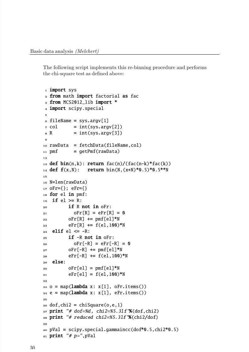
The following script implements this re-binning procedure and performsthe chi-square test as defined above:
1 import sys
2 from math import factorial as fac
3 from MCS2012_lib import *
4 import scipy.special
5
6 fileName = sys.argv[1]
7 col = int(sys.argv[2])
8 R = int(sys.argv[3])
9
10 rawData = fetchData(fileName,col)
11 pmf = getPmf(rawData)
12
13 def bin(n,k): return fac(n)/(fac(n-k)*fac(k))
14 def f (x,N): return bin(N,(x+N)*0.5)*0.5**N
15
16 N=len(rawData)
17 oFr=; eFr=
18 for el in pmf:
19 if el >= R:
20 if R not in oFr:
21 oFr[R] = eFr[R] = 0
22 oFr[R] += pmf[el]*N
23 eFr[R] += f(el,100)*N
24 elif el <= -R:
25 if -R not in oFr:
26 oFr[-R] = eFr[-R] = 0
27 oFr[-R] += pmf[el]*N
28 eFr[-R] += f(el,100)*N
29 else:
30 oFr[el] = pmf[el]*N
31 eFr[el] = f(el,100)*N
32
33 o = map(lambda x: x[1], oFr.items())
34 e = map(lambda x: x[1], eFr.items())
35
36 dof,chi2 = chiSquare(o,e,1)
37 print "# dof=%d , chi2=%5.3lf " % (dof,chi2)
38 print "# reduced chi2=%5.3lf " % (chi2/dof)
39
40 pVal = scipy.special.gammaincc(dof *0.5,chi2*0.5)
41 print "# p=" ,pVal
7/27/2019 Big Data Analysis using Python
http://slidepdf.com/reader/full/big-data-analysis-using-python 31/62
3 Object oriented programming in python
Therein, in lines 13–14, the symmetric binomial distribution is defined,and in lines 16–31 the re-binning of the data is carried out. Finally, lines33–34 prepare the re-binned data for the chi-sqare test (line 36). Notethat the script above extends the chi-square goodness-of-fit test by alsocomputing the so-called p-value for the problem at hand (line 40). The
p-value is a standard way to assess the significance of the chi-square test,see Refs. [17, 20]. In essence, the numerical value of p gives the proba-bility that the sum of the squares of a number of dof Gaussian randomvariables (zero mean and unit variance) will be greater than χ2. To com-
pute the p-value an implementation of the incomplete gamma function isneeded. Unfortunately, this is not contained in a standard python pack-age. However, the incomplete gamma function is available through thescipy-package [6], which offers an extensive selection of special functionsand lots of scientific tools. Considering the p-value, the observed frequen-cies are consistent with the expected frequencies, if the numerical value of
p is not smaller than, say, 10−2.
If the script is called for R = 40 it yields the result:
1 > python chiSquare.py N100_n100000.dat 1 40
2
# dof=40, chi2=38.2563 # reduced chi2=0.956
4 # p= 0.549
Hence, the pmf for the end point distribution of the symmetric 1D randomwalk appears to be consistent with the symmetric binomial distributionwith mean 0 and variance N/4, wherein N specifies the number of stepsin a single walk.
3 Object oriented programming in pythonIn addition to the built-in data types used earlier in these notes, python allows youto define your own custom data structures. In doing so, python makes it easy tofollow an object oriented programming (OOP) approach. The basic idea of the OOPapproach is to use objects in order to design computer programs. Therein, the term’object’ refers to a custom data structure that has certain attributes and methods ,where the latter can be understood as functions that alter the attributes of the datastructure.
By following an OOP approach, the first step consists in putting the problem athand under scrutiny and figuring out what the respective objects might be. Once
this first step is accomplished one might go on and design custom data structures torepresent the objects. In python this is done using the concept of classes .
In general, OOP techniques emphasize on data encapsulation , inheritance , andoverloading . In less formal terms, data encapsulation means to ’hide the implemen-tation’. I.e., the access to the attributes of the data structures is typically restricted,
7/27/2019 Big Data Analysis using Python
http://slidepdf.com/reader/full/big-data-analysis-using-python 32/62
Basic data analysis (Melchert)
making them (somewhat) private . Access to the attributes is only granted for certainmethods that build an interface by means of which an user can alter the attributes.The concept of data encapsulation slightly interferes with the ’everything is public’consensus of the python community which follows the habit that even if one mightbe able to see the implementation one does not have to care about it. Nevertheless,python offers a kind of pseudo-encapsulation referred to as name-mangling which willbe illustrated in Subsection 3.2
In OOP terms, inheritance means to ’share code among classes’. It highly encour-ages code recycling and easily allows to extend or specialize existing classes, thereby
generating a hierarchy composed of classes and derived subclasses .Finally, overloading means to ’redefine methods on subclass level’. This makes it
possible to adapt methods to their context. Also known as polymorphism , this offersthe possibility to have several definitions of the same method on different levels of theclass hierarchy.
3.1 Implementing an undirected graph
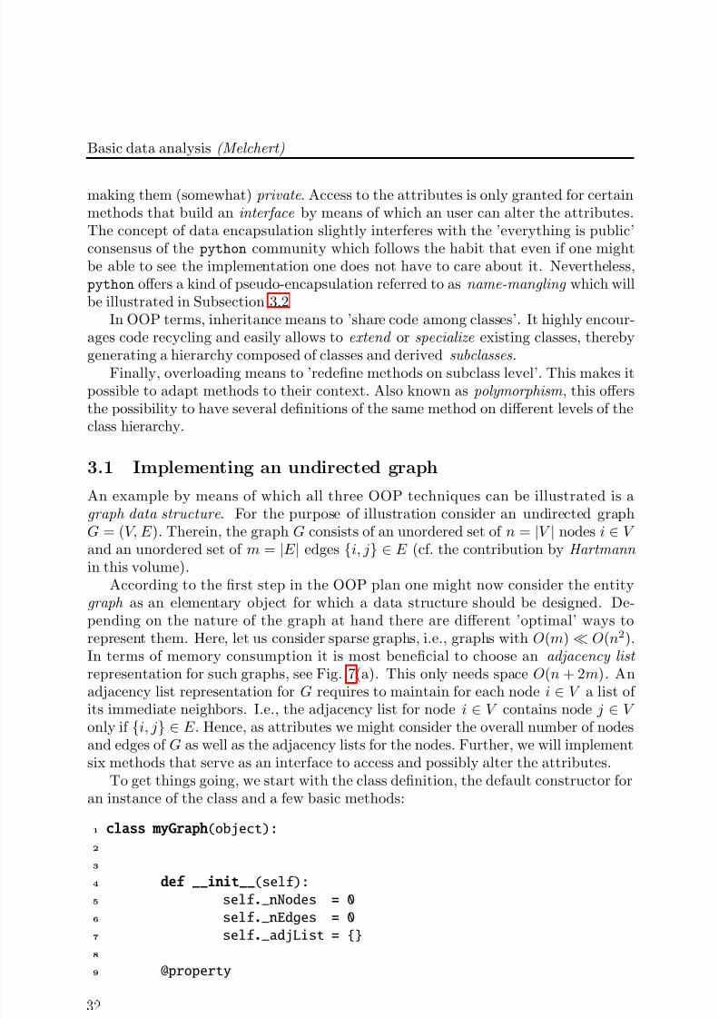
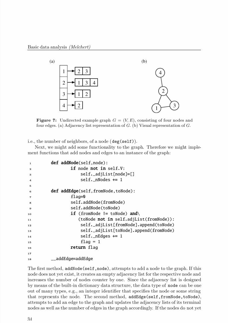
An example by means of which all three OOP techniques can be illustrated is agraph data structure . For the purpose of illustration consider an undirected graph
G = (V, E ). Therein, the graph G consists of an unordered set of n = |V | nodes i ∈ V and an unordered set of m = |E | edges i, j ∈ E (cf. the contribution by Hartmann in this volume).
According to the first step in the OOP plan one might now consider the entitygraph as an elementary object for which a data structure should be designed. De-pending on the nature of the graph at hand there are different ’optimal’ ways torepresent them. Here, let us consider sparse graphs, i.e., graphs with O(m) O(n2).In terms of memory consumption it is most beneficial to choose an adjacency list representation for such graphs, see Fig. 7(a). This only needs space O(n + 2m). Anadjacency list representation for G requires to maintain for each node i ∈ V a list of
its immediate neighbors. I.e., the adjacency list for node i ∈ V contains node j ∈ V only if i, j ∈ E . Hence, as attributes we might consider the overall number of nodesand edges of G as well as the adjacency lists for the nodes. Further, we will implementsix methods that serve as an interface to access and possibly alter the attributes.
To get things going, we start with the class definition, the default constructor foran instance of the class and a few basic methods:
1 class myGraph(object):
2
3
4 def __init__(self):
5 self ._nNodes = 0
6 self ._nEdges = 0
7 self ._adjList =
8
9 @property
7/27/2019 Big Data Analysis using Python
http://slidepdf.com/reader/full/big-data-analysis-using-python 33/62
3 Object oriented programming in python
10 def nNodes(self):
11 return self ._nNodes
12
13 @nNodes.setter
14 def nNodes(self,val):
15 print "will not change private attribute"
16
17 @property
18 def nEdges(self):
19 return self ._nEdges20
21 @nEdges.setter
22 def nEdges(self,val):
23 print "will not change private attribute"
24
25 @property
26 def V(self):
27 return self ._adjList.keys()
28
29 def adjList(self,node):30 return self ._adjList[node]
31
32 def deg(self,node):
33 return len(self ._adjList[node])
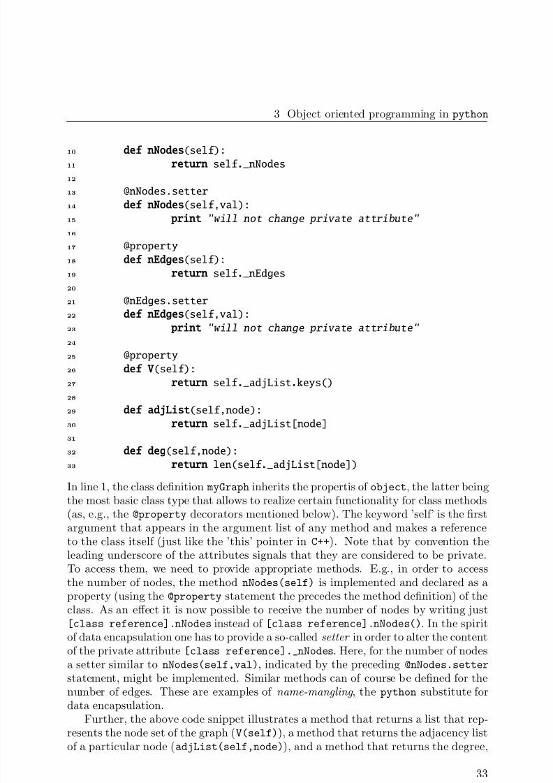
In line 1, the class definition myGraph inherits the propertis of object, the latter beingthe most basic class type that allows to realize certain functionality for class methods(as, e.g., the @property decorators mentioned below). The keyword ’self’ is the firstargument that appears in the argument list of any method and makes a referenceto the class itself (just like the ’this’ pointer in C++). Note that by convention theleading underscore of the attributes signals that they are considered to be private.To access them, we need to provide appropriate methods. E.g., in order to accessthe number of nodes, the method nNodes(self) is implemented and declared as aproperty (using the @property statement the precedes the method definition) of theclass. As an effect it is now possible to receive the number of nodes by writing just[class reference].nNodes instead of [class reference].nNodes(). In the spiritof data encapsulation one has to provide a so-called setter in order to alter the contentof the private attribute [class reference]._nNodes. Here, for the number of nodesa setter similar to nNodes(self,val), indicated by the preceding @nNodes.setter
statement, might be implemented. Similar methods can of course be defined for the
number of edges. These are examples of name-mangling , the python substitute fordata encapsulation.
Further, the above code snippet illustrates a method that returns a list that rep-resents the node set of the graph (V(self)), a method that returns the adjacency listof a particular node (adjList(self,node)), and a method that returns the degree,
7/27/2019 Big Data Analysis using Python
http://slidepdf.com/reader/full/big-data-analysis-using-python 34/62
Basic data analysis (Melchert)
(a) (b)
22
1 4
13
41 2 3
4
3
2 3
2
1
Figure 7: Undirected example graph G = (V, E ), consisting of four nodes andfour edges. (a) Adjacency list representation of G. (b) Visual representation of G.
i.e., the number of neighbors, of a node (deg(self)).Next, we might add some functionality to the graph. Therefore we might imple-
ment functions that add nodes and edges to an instance of the graph:
1 def addNode(self,node):
2
if node not in self .V:3 self ._adjList[node]=[]
4 self ._nNodes += 1
5
6 def addEdge(self,fromNode,toNode):
7 flag=0
8 self .addNode(fromNode)
9 self .addNode(toNode)
10 if (fromNode != toNode) and\
11 (toNode not in self .adjList(fromNode)):
12
self ._adjList[fromNode].append(toNode)13 self ._adjList[toNode].append(fromNode)
14 self ._nEdges += 1
15 flag = 1
16 return flag
17
18 __addEdge=addEdge
The first method, addNode(self,node), attempts to add a node to the graph. If thisnode does not yet exist, it creates an empty adjacency list for the respective node andincreases the number of nodes counter by one. Since the adjacency list is designed
by means of the built-in dictionary data structure, the data type of node can be oneout of many types, e.g., an integer identifier that specifies the node or some stringthat represents the node. The second method, addEdge(self,fromNode,toNode),attempts to add an edge to the graph and updates the adjacency lists of its terminalnodes as well as the number of edges in the graph accordingly. If the nodes do not yet
7/27/2019 Big Data Analysis using Python
http://slidepdf.com/reader/full/big-data-analysis-using-python 35/62
3 Object oriented programming in python
exist, it creates them first by calling the addNode() method. Note that the addEdge()
method returns a value of zero if the edge exists already and returns a value of one if the edge did not yet exist. Further, the last line in the code snippet above constructsa local copy of the method. Neither the use of the edge existence flag, nor the use of the local copy is obvious at the moment. Both we will be clarified below.
To make the graph class even more flexible we might amend it by implementingmethods that delete nodes and edges:
1 def delNode(self,node):
2
for nb in [nbNodes for nbNodes in\3 self ._adjList[node]]:
4 self .delEdge(nb,node)
5 del self ._adjList[node]
6 self ._nNodes -= 1
7
8 def delEdge(self,fromNode,toNode):
9 flag = 0
10 if fromNode in self .adjList(toNode):
11 self ._adjList[fromNode].remove(toNode)
12
self ._adjList[toNode].remove(fromNode)13 self ._nEdges -= 1
14 flag = 1
15 return flag
16
17 __delEdge=delEdge
In the above code snippet, the method delNode(self,node) deletes a supplied nodefrom the adjacency lists of all its neighbors, deletes the adjacency list of the nodeand finally decreases the number of nodes in the graph by one. The second method,called delEdge(self,fromNode,toNode), deletes an edge from the graph. Therefore,it modifies the adjacency lists of its terminal nodes and decreases the number of edgesin the graph by one.
As a last point, we might want to print the graph. For that purpose we mightimplement the method __str__(self) that is expected to compute a string rep-resentation of the graph object, to return the graph as string using the graphviz
dot-language [7]:
1 def __str__(self):
2 string = ’graph G \
3 \n rankdir=LR;\
4 \n node [shape = circle,size=0.5];\
5 \n // graph attributes:\
6 \n // nNodes=%d\
7 \n // nEdges=%d\
8 \n’ % (self .nNodes,self .nEdges)
7/27/2019 Big Data Analysis using Python
http://slidepdf.com/reader/full/big-data-analysis-using-python 36/62
Basic data analysis (Melchert)
9
10 # for a more clear presentation:
11 # write node list fist
12 string += ’\n // node-list:\n’
13 for n in self .V:
14 string += ’ %s; // deg=%d\n’ % \
15 (str(n),self .deg(n))
16
17 # write edge list second
18 string += ’\n // edge-list:\n’19 for n1 in self .V:
20 for n2 in self .adjList(n1):
21 if n1<n2:
22 string += ’ %s -- %s [len=1.5];\n’ % \
23 (str(n1),str(n2))
24 string += ’’
25 return string
A small script that illustrates some of the graph class functionality is easily written(graphExample.py):
1 from undirGraph_oop import *
2
3 g = myGraph()
4
5 g.addEdge(1,1)
6 g.addEdge(1,2)
7 g.addEdge(1,3)
8 g.addEdge(2,3)
9 g.addEdge(2,4)
10
11 print g
Invoking the script on the command-line yields the graph in terms of the dot-language:
1 > python graphExample.py
2 graph G
3 rankdir=LR;
4 node [shape = circle,size=0.5];
5 // graph attributes:
6 // nNodes=4
7 // nEdges=48
9 // node-list:
10 1; // deg=2
11 2; // deg=3
7/27/2019 Big Data Analysis using Python
http://slidepdf.com/reader/full/big-data-analysis-using-python 37/62
3 Object oriented programming in python
12 3; // deg=2
13 4; // deg=1
14
15 // edge-list:
16 1 - - 2 [len=1.5];
17 1 - - 3 [len=1.5];
18 2 - - 3 [len=1.5];
19 2 - - 4 [len=1.5];
20
Using the graph drawing command-line tools provided by the graphviz library, thegraph can be post-processed to yield Fig. 7(b). For that, simply pipe the dot-language description of the graph to a file, say graph.dot and post-process the filevia neato -Tpdf graph.dot > graph.pdf to generate the pdf file that contains avisual representation of the graph.
Further, we might use the class myGraph as an base class to set up a subclass myWeightedGraph, allowing to handle graphs with edge weights. The respective classdefinition along with the default constructor for an instance of the class and somebasic methods are listed below:
1 class myWeightedGraph(myGraph):2 def __init__(self):
3 myGraph.__init__(self)
4 self ._wgt =
5
6 @property
7 def E(self):
8 return self ._wgt.keys()
9
10 def wgt(self,fromNode,toNode):
11 sortedEdge = (min(fromNode,toNode),\12 max(fromNode,toNode))
13 return self ._wgt[sortedEdge]
14
15 def setWgt(self,fromNode,toNode,wgt):
16 if toNode in self .adjList(fromNode):
17 sortedEdge = (min(fromNode,toNode),\
18 max(fromNode,toNode))
19 self ._wgt[sortedEdge]=wgt
Therein, the way in which the new class myWeightedGraph incorporates the exist-
ing class myGraph is an example for inheritance . In this manner, myWeightedGraphextends the existing graph class by edge weights that will be stored in the dictio-nary self._wgt. In the default constructor, the latter is introduced as a privateclass attribute. Further, the code snippet shows three new methods that are im-plemented to extend the base class. For the edge weight dictionary, it is necessary
7/27/2019 Big Data Analysis using Python
http://slidepdf.com/reader/full/big-data-analysis-using-python 38/62
Basic data analysis (Melchert)
to explicitly store the edges, hence it comes at no extra ’cost’ to provide a method(E(self)) that serves to return a list of all edges in the graph. Further, the methodwgt(self,fromNode,toNode) reports the weight of an edge if this exists already andthe method setWgt(self,fromNode,toNode,wgt) sets the weight of an edge if thelatter exists already.
Unfortunately, the existing base class methods for adding and deleting edges can-not be used in the ’extended’ context of weighted graphs. They have to be redefined inorder to also make an entry in the edge weight dictionary once an edge is constructed.As an example for the OOP aspect of function overloading , this is illustrated in the
following code snippet:
1 def addEdge(self,fromNode,toNode,wgt=1):
2 if self ._myGraph__addEdge(fromNode,toNode):
3 self .setWgt(fromNode,toNode,wgt)
4
5 def delEdge(self,fromNode,toNode):
6 if self ._myGraph__delEdge(fromNode,toNode):
7 sortedEdge = (min(fromNode,toNode),\
8 max(fromNode,toNode))
9 del self ._wgt[sortedEdge]
There are two things to note. First, an odd-named method _myGraph__addEdge() iscalled. This simply refers to the local copy __addEdge() of the addEdge() methodon the level of the base class (hence the preceeing _myGraph). This is still intact,even though the method addEdge() is overloaded on the current level of the classhierarchy. Second, the previously introduced edge-existence flag is utilized to makean entry in the weight dictionary only if the edge is constructed during the currentfunction call. In order to change an edge weight later on, the setWgt() method mustbe used.
This completes the exemplary implementation of a graph data structure to il-lustrate the three OOP techniques of data encapsulation, inheritance, and functionoverloading.
3.2 A simple histogram data structure
An example that is more useful for the purpose of data analysis is presented below( myHist_oop.py). We will implement a histogram data structure that performs thesame task as the hist_linBinning() function implemented in Section 2.2, only inOOP style.
7/27/2019 Big Data Analysis using Python
http://slidepdf.com/reader/full/big-data-analysis-using-python 39/62
3 Object oriented programming in python
1 from math import sqrt,floor
2
3 class simpleStats(object):
4 def __init__(self):
5 self ._N =0
6 self ._av =0.
7 self ._Q =0.
8
9 def add(self,val):
10 self ._N+=1
11 dum = val-self ._av
12 self ._av+= float(dum)/self ._N
13 self ._Q+=dum *(val-self ._av)
14
15 @property
16 def av(self): return self ._av
17
18 @property
19 def sDev(self): return sqrt(self ._Q/(self ._N-1))
20
21 @property
22 def sErr(self): return self .sDev/sqrt(self ._N)
23
24
25 class myHist(object):
26
27 def __init__(self,xMin,xMax,nBins):
28 self ._min = min(xMin,xMax)
29 self ._max = max(xMin,xMax)
30 self ._cts = 0
31 self ._nBins = nBins
32
33 self ._bin = [0]*(nBins+2)
34 self ._norm = None
35 self ._dx = \
36 float(self ._max-self ._min)/self ._nBins
37
38 self ._stats = simpleStats()
39
40 def __binId(self,val):
41 return int(floor((val-self ._min)/self ._dx))
42
43 def __bdry(self,bin):
44 return self ._min+bin*self ._dx,\
7/27/2019 Big Data Analysis using Python
http://slidepdf.com/reader/full/big-data-analysis-using-python 40/62
7/27/2019 Big Data Analysis using Python
http://slidepdf.com/reader/full/big-data-analysis-using-python 41/62
3 Object oriented programming in python
In the above code snippet, the first class definition (line 3) defines the data struc-ture simple statistics. It implements methods to compute the average, standarddeviation and standard error of the supplied values in single-pass fashion. Numericalvalues are added by calling the class method add(), defined in lines 9–13.
The second class definition (line 25) belongs to the histogram data structure. Theclass implements a histogram using linear binning of the supplied data. It computesthe probability density function that approximates the supplied data and furtherprovides some simple statistics such as average, standard deviation and standarderror.
Upon initialization an instance of the class requires three numerical values, asevident from the default constructor for an instance of the class (lines 27–38). Theseare xMin, a lower bound (inclusive) on values that are considered in order to accu-mulate frequency statistics for the histogram, xMax, an upper bound (exclusive) onvalues that are considered to accumulate frequency statistics for the histogram, andnBins, the number of bins used to set up the histogram. All values x that are eithersmaller than xMin or greater or equal to xMax are not considered for the calculationof frequency statistics, but are considered for the normalization of the histogram toyield a probability density function (pdf). Further, all values are used to computethe average, standard deviation and standard error.
In the scope of the histogram class, several “private” methods are defined (signifiedby preceding double underscores), that, e.g., compute the integer identifier of the binthat corresponds to a supplied numerical value (lines 40–41), compute upper andlower boundaries of a bin (lines 43–45), compute a Gaussian error bar for each bin(lines 47–49), and normalize the frequency statistics to yield a probability density(lines 51–53).
Further, the user interface consists of four methods, the first three of which areav(), sDev(), and sErr(), providing access to the mean, standard deviation, andstandard error of the supplied values, respectively. Most important, lines 64–72 imple-ment the fourth method addValue(), that adds a value to the histogram and updates
the frequencies and overall statistics accordingly. Finally, lines 74–88 implement thestring representation of the histogram class.As an example, we might generate a histogram from the data of the 2D random
walks using the myHist_oop class (rw2D_hist_oop.py):
1 import sys
2 from myHist_oop import myHist
3 from MCS2012_lib import fetchData
4
5 def main():
6 ## parse command line args
7 fName = sys.argv[1]
8 col = int(sys.argv[2])
9 nBins = int(sys.argv[3])
10
11 ## get data from file
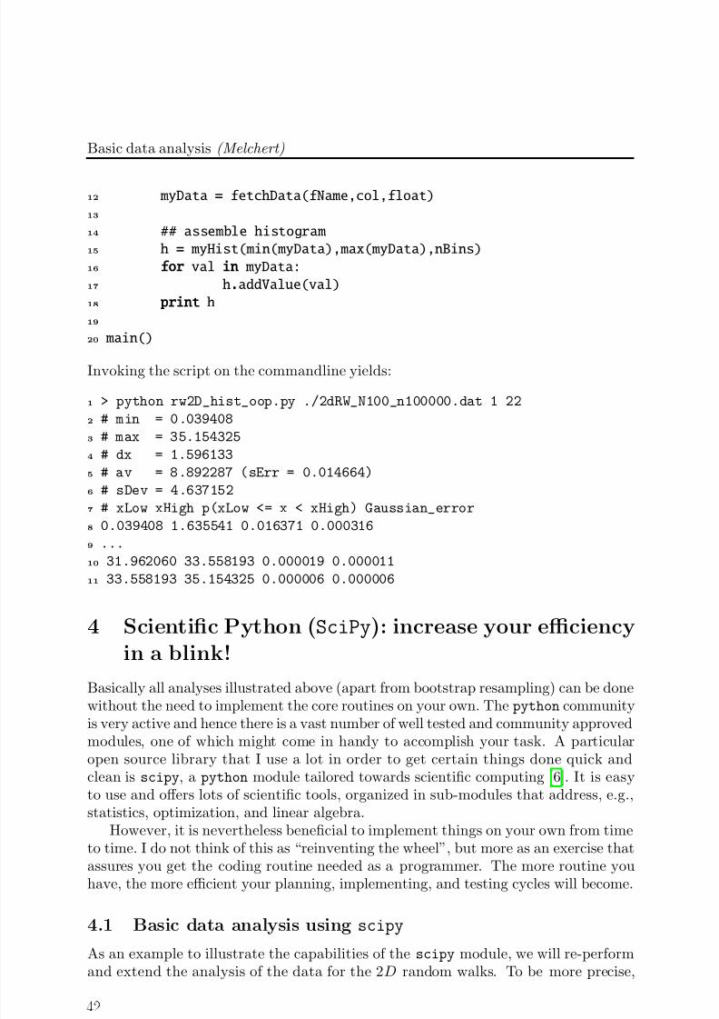
7/27/2019 Big Data Analysis using Python
http://slidepdf.com/reader/full/big-data-analysis-using-python 42/62
Basic data analysis (Melchert)
12 myData = fetchData(fName,col,float)
13
14 ## assemble histogram
15 h = myHist(min(myData),max(myData),nBins)
16 for val in myData:
17 h.addValue(val)
18 print h
19
20 main()
Invoking the script on the commandline yields:
1 > python rw2D_hist_oop.py ./2dRW_N100_n100000.dat 1 22
2 # min = 0.039408
3 # max = 35.154325
4 # dx = 1.596133
5 # av = 8.892287 (sErr = 0.014664)
6 # sDev = 4.637152
7 # xLow xHigh p(xLow <= x < xHigh) Gaussian_error
8 0.039408 1.635541 0.016371 0.000316
9 ...
10 31.962060 33.558193 0.000019 0.000011
11 33.558193 35.154325 0.000006 0.000006
4 Scientific Python (SciPy): increase your efficiencyin a blink!
Basically all analyses illustrated above (apart from bootstrap resampling) can be donewithout the need to implement the core routines on your own. The python communityis very active and hence there is a vast number of well tested and community approvedmodules, one of which might come in handy to accomplish your task. A particularopen source library that I use a lot in order to get certain things done quick andclean is scipy, a python module tailored towards scientific computing [6]. It is easyto use and offers lots of scientific tools, organized in sub-modules that address, e.g.,statistics, optimization, and linear algebra.
However, it is nevertheless beneficial to implement things on your own from timeto time. I do not think of this as “reinventing the wheel”, but more as an exercise thatassures you get the coding routine needed as a programmer. The more routine youhave, the more efficient your planning, implementing, and testing cycles will become.
4.1 Basic data analysis using scipy
As an example to illustrate the capabilities of the scipy module, we will re-performand extend the analysis of the data for the 2D random walks. To be more precise,
7/27/2019 Big Data Analysis using Python
http://slidepdf.com/reader/full/big-data-analysis-using-python 43/62
4 Increase your efficiency using Scientific Python (scipy)
we will compute basic parameters related to the data, generate a histogram to yielda pdf of the geometric distance RN the walkers traveled after N = 100 steps, andperform a χ2 goodness-of-fit test to assess whether the approximate pdf appears tobe equivalent to a Rayleigh distribution. A full script to perform the above analysesusing the scipy module reads (rw2d_analysis_scipy.py):
1 import sys
2 import scipy
3 import scipy.stats as sciStat
4 from MCS2012_lib import fetchData
5
6 def myPdf (x): return sciStat.rayleigh.pdf(x,scale=sigma)
7 def myCdf (x): return sciStat.rayleigh.cdf(x,scale=sigma)
8
9 fileName = sys.argv[1]
10 nBins = int(sys.argv[2])
11
12 rawData = fetchData(fileName,1,float)
13
14 print ’## Basic statistics using scipy’
15 print ’# data file:’, fileName
16 N = len(rawData)
17 sigma = scipy.sqrt(sum(map(lambda x:x*x,rawData))*0.5/N)
18 av = scipy. mean(rawData)
19 sDev = scipy.std(rawData)
20 print ’# N =’, N
21 print ’# av =’, av
22 print ’# sDev =’, sDev
23 print ’# sigma =’, sigma
24
25 print ’## Histogram using scipy’
26 limits = (min(rawData),max(rawData))
27 freqObs,xMin,dx,nOut =\
28 sciStat.histogram(rawData,nBins,limits)
29 bdry = [(xMin+i*dx ,xMin+(i+1)*dx) for i in range(nBins)]
30
31 print ’# nBins = ’, nBins
32 print ’# xMin = ’, xMin
33 print ’# dx = ’, dx
34 print ’# (binCenter) (pdf-observed) (pdf-rayleigh distrib.)’
35 for i in range(nBins):
36 x = 0.5*(bdry[i][0]+bdry[i][1])
37 print x, freqObs[i]/(N*dx), myPdf(x)
38
39 print ’## Chi2 - test using scipy’
7/27/2019 Big Data Analysis using Python
http://slidepdf.com/reader/full/big-data-analysis-using-python 44/62
Basic data analysis (Melchert)
40 freqExp = scipy.array(
41 [N*(myCdf(x[1])- myCdf(x[0])) for x in bdry])
42
43 chi2,p = sciStat.chisquare(freqObs,freqExp,ddof =1)
44 print ’# chi2 = ’, chi2
45 print ’# chi2/dof = ’, chi2/(nBins-1)
46 print ’# pVal = ’, p
In lines 2 and 3, the scipy module and its submodule scipy.stats are imported.The latter contains a large number of discrete and continuous probability distributions(that allow to draw random variates, or to evaluate the respective pdf and cdf) anda huge library of statistical functions. E.g., in lines 18 and 19 we use the scipy
functions scipy.mean(rawData) and scipy.std(rawData), respectively, to computethe mean and standard deviation of the individual values of RN stored in the arrayrawData.
However, be aware that the function scipy.std(x) computes the square-rootof the uncorrected variance uVar(x) = av([x − av(x)]2). Hence, the scipy imple-mentation of the above function yields no unbiased estimate of the standard de-viation. An unbiased estimate of the standard deviation can be obtained usingscipy.sqrt(N/(N-1))*scipy.std(x), where N=len(x).
Next, in lines 25–37 a pdf of the geometric distance RN is computed. Therefore,in lines 27–28, a frequency histogram for the raw data is calculated using the functionscipy.stats.histogram(). As arguments, the function takes the array rawData
with events that are to be binned, the integer nBins specifying the number of his-togram bins, and the tuple limits, holding the upper and lower limits of the histogramrange. The histogram function returns the four-tuple freqObs,xMin,dx,nOut, wherefreqObs is an array containing the number of events for the individual bins, xMin isthe lower boundary value of the smallest bin, dx is the bin width, and nOut countsthe number of events that fall not within the range of the histogram. In line 29 theboundary values of all individual bins are reconstructed from the output of the his-togram function by means of a list comprehension (i.e. an inline looping construct).In lines 35–37, the frequencies are transformed to probability densities and listed asfunction of the bin centers. As discussed earlier (see the example on the continuous2D random walk in Section 2.1), for N large enough, RN is properly described bythe Rayleigh distribution with shape parameter σ. In order to facilitate a compari-son of the observed pdf to the pdf thus expected, the scipy probability distributionscipy.stats.rayleigh.pdf(x,shape=sigma), abbreviated as myPdf(x) in line 6, islisted, too.
From the corresponding cumulative distribution function (abbreviated myCdf(x)
in line 7), scipy.stats.rayleigh.cdf(x,shape=sigma), the expected number of
events within each bin is computed in lines 40–41. Finally, in line 43, and by using thefunction scipy.stats.chisquare(), a chi-square goodness-of-fit test is performed toassess whether the observed distribution is in agreement with the expected limitingdistribution. In the above function, the first two arguments refer to the observed andexpected frequencies of events, respectively, and the parameter ddof serves to adjust
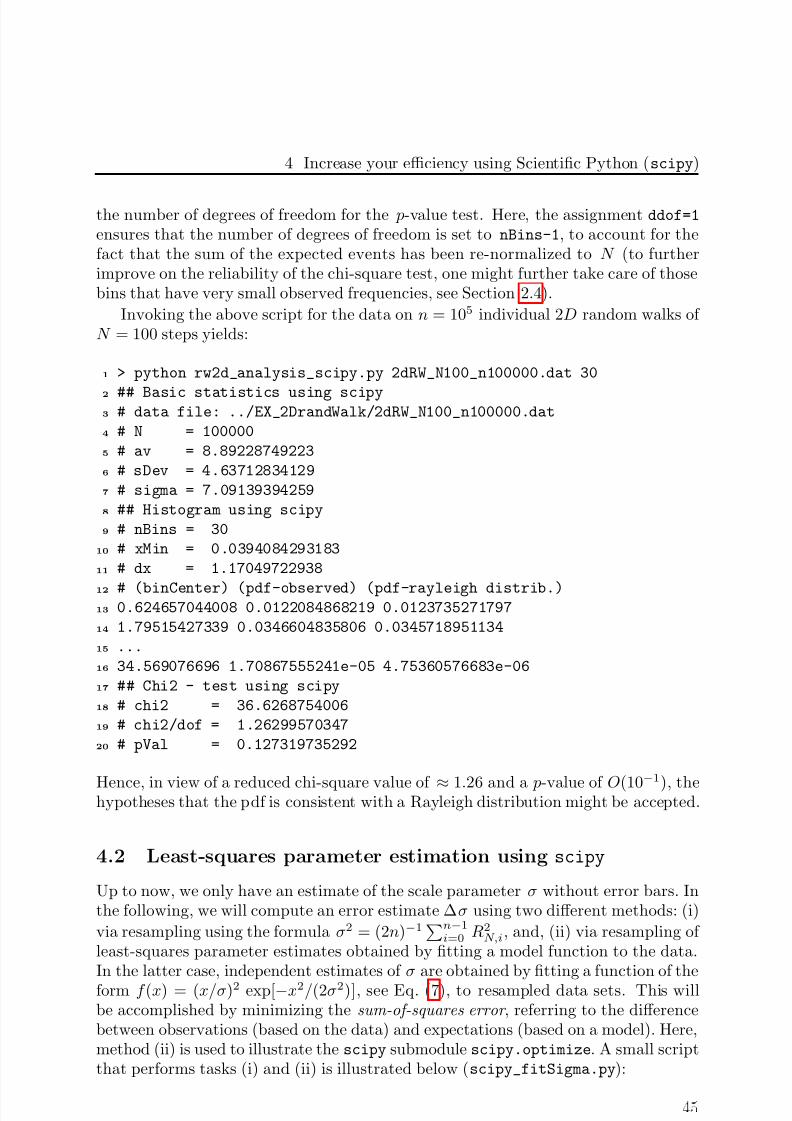
7/27/2019 Big Data Analysis using Python
http://slidepdf.com/reader/full/big-data-analysis-using-python 45/62
4 Increase your efficiency using Scientific Python (scipy)
the number of degrees of freedom for the p-value test. Here, the assignment ddof=1
ensures that the number of degrees of freedom is set to nBins-1, to account for thefact that the sum of the expected events has been re-normalized to N (to furtherimprove on the reliability of the chi-square test, one might further take care of thosebins that have very small observed frequencies, see Section 2.4).
Invoking the above script for the data on n = 105 individual 2D random walks of N = 100 steps yields:
1 > python rw2d_analysis_scipy.py 2dRW_N100_n100000.dat 30
2 ## Basic statistics using scipy3 # data file: ../EX_2DrandWalk/2dRW_N100_n100000.dat
4 # N = 100000
5 # av = 8.89228749223
6 # sDev = 4.63712834129
7 # sigma = 7.09139394259
8 ## Histogram using scipy
9 # nBins = 30
10 # xMin = 0.0394084293183
11 # dx = 1.17049722938
12 # (binCenter) (pdf-observed) (pdf-rayleigh distrib.)13 0.624657044008 0.0122084868219 0.0123735271797
14 1.79515427339 0.0346604835806 0.0345718951134
15 ...
16 34.569076696 1.70867555241e-05 4.75360576683e-06
17 ## Chi2 - test using scipy
18 # chi2 = 36.6268754006
19 # chi2/dof = 1.26299570347
20 # pVal = 0.127319735292
Hence, in view of a reduced chi-square value of ≈ 1.26 and a p-value of O(10−1
), thehypotheses that the pdf is consistent with a Rayleigh distribution might be accepted.
4.2 Least-squares parameter estimation using scipy
Up to now, we only have an estimate of the scale parameter σ without error bars. Inthe following, we will compute an error estimate ∆σ using two different methods: (i)
via resampling using the formula σ2 = (2n)−1n−1
i=0 R2N,i, and, (ii) via resampling of
least-squares parameter estimates obtained by fitting a model function to the data.In the latter case, independent estimates of σ are obtained by fitting a function of the
form f (x) = (x/σ)2 exp[−x2/(2σ2)], see Eq. (7), to resampled data sets. This willbe accomplished by minimizing the sum-of-squares error , referring to the differencebetween observations (based on the data) and expectations (based on a model). Here,method (ii) is used to illustrate the scipy submodule scipy.optimize. A small scriptthat performs tasks (i) and (ii) is illustrated below (scipy_fitSigma.py):
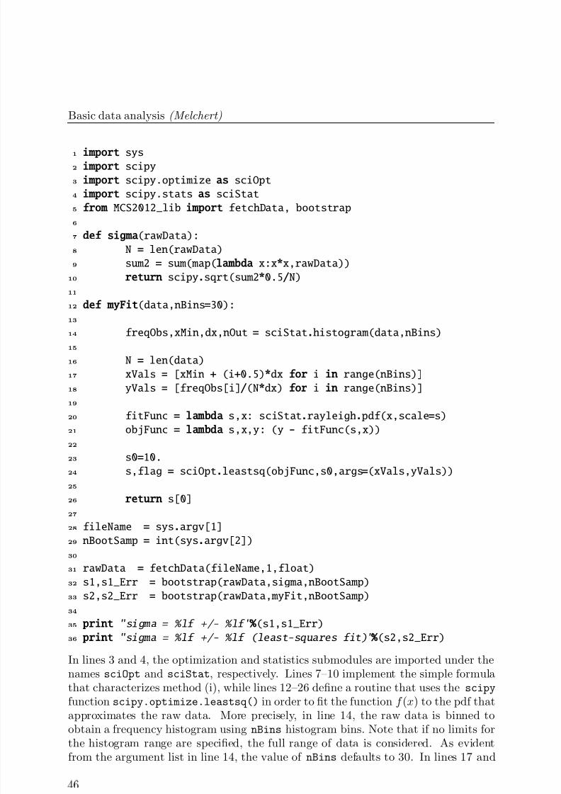
7/27/2019 Big Data Analysis using Python
http://slidepdf.com/reader/full/big-data-analysis-using-python 46/62
Basic data analysis (Melchert)
1 import sys
2 import scipy
3 import scipy.optimize as sciOpt
4 import scipy.stats as sciStat
5 from MCS2012_lib import fetchData, bootstrap
6
7 def sigma(rawData):
8 N = len(rawData)
9 sum2 = sum(map(lambda x:x*x,rawData))
10 return scipy.sqrt(sum2*0.5/N)11
12 def myFit(data,nBins=30):
13
14 freqObs,xMin,dx,nOut = sciStat.histogram(data,nBins)
15
16 N = len(data)
17 xVals = [xMin + (i+0.5)*dx for i in range(nBins)]
18 yVals = [freqObs[i]/(N*dx) for i in range(nBins)]
19
20 fitFunc = lambda s,x: sciStat.rayleigh.pdf(x,scale=s)21 objFunc = lambda s,x,y: (y - fitFunc(s,x))
22
23 s0=10.
24 s,flag = sciOpt.leastsq(objFunc,s0,args=(xVals,yVals))
25
26 return s[0]
27
28 fileName = sys.argv[1]
29 nBootSamp = int(sys.argv[2])
30
31 rawData = fetchData(fileName,1,float)
32 s1,s1_Err = bootstrap(rawData,sigma,nBootSamp)
33 s2,s2_Err = bootstrap(rawData,myFit,nBootSamp)
34
35 print "sigma = %lf +/- %lf " % (s1,s1_Err)
36 print "sigma = %lf +/- %lf (least-squares fit)" % (s2,s2_Err)
In lines 3 and 4, the optimization and statistics submodules are imported under thenames sciOpt and sciStat, respectively. Lines 7–10 implement the simple formulathat characterizes method (i), while lines 12–26 define a routine that uses the scipy
function scipy.optimize.leastsq() in order to fit the function f (x) to the pdf thatapproximates the raw data. More precisely, in line 14, the raw data is binned toobtain a frequency histogram using nBins histogram bins. Note that if no limits forthe histogram range are specified, the full range of data is considered. As evidentfrom the argument list in line 14, the value of nBins defaults to 30. In lines 17 and
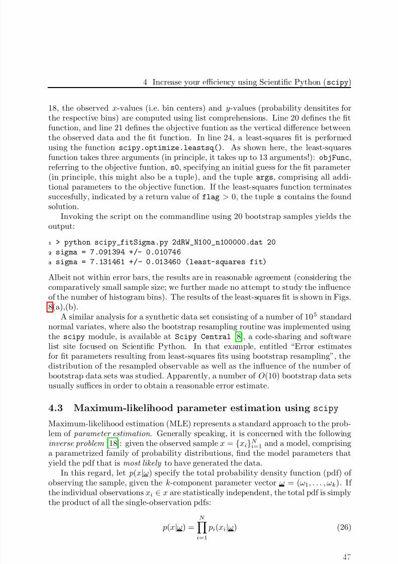
7/27/2019 Big Data Analysis using Python
http://slidepdf.com/reader/full/big-data-analysis-using-python 47/62
4 Increase your efficiency using Scientific Python (scipy)
18, the observed x-values (i.e. bin centers) and y-values (probability densitites forthe respective bins) are computed using list comprehensions. Line 20 defines the fitfunction, and line 21 defines the objective funtion as the vertical difference betweenthe observed data and the fit function. In line 24, a least-squares fit is performedusing the function scipy.optimize.leastsq(). As shown here, the least-squaresfunction takes three arguments (in principle, it takes up to 13 arguments!): objFunc,referring to the objective funtion, s0, specifying an initial guess for the fit parameter(in principle, this might also be a tuple), and the tuple args, comprising all addi-tional parameters to the objective function. If the least-squares function terminates
succesfully, indicated by a return value of flag > 0, the tuple s contains the foundsolution.
Invoking the script on the commandline using 20 bootstrap samples yields theoutput:
1 > python scipy_fitSigma.py 2dRW_N100_n100000.dat 20
2 sigma = 7.091394 +/- 0.010746
3 sigma = 7.131461 +/- 0.013460 (least-squares fit)
Albeit not within error bars, the results are in reasonable agreement (considering thecomparatively small sample size; we further made no attempt to study the influence
of the number of histogram bins). The results of the least-squares fit is shown in Figs.8(a),(b).
A similar analysis for a synthetic data set consisting of a number of 105 standardnormal variates, where also the bootstrap resampling routine was implemented usingthe scipy module, is available at Scipy Central [8], a code-sharing and softwarelist site focused on Scientific Python. In that example, entitled “Error estimatesfor fit parameters resulting from least-squares fits using bootstrap resampling”, thedistribution of the resampled observable as well as the influence of the number of bootstrap data sets was studied. Apparently, a number of O(10) bootstrap data setsusually suffices in order to obtain a reasonable error estimate.
4.3 Maximum-likelihood parameter estimation using scipy
Maximum-likelihood estimation (MLE) represents a standard approach to the prob-lem of parameter estimation . Generally speaking, it is concerned with the followinginverse problem [18]: given the observed sample x = xiN i=1 and a model, comprisinga parametrized family of probability distributions, find the model parameters thatyield the pdf that is most likely to have generated the data.
In this regard, let p(x|ω) specify the total probability density function (pdf) of observing the sample, given the k-component parameter vector ω = (ω1, . . . , ωk). If
the individual observations xi ∈ x are statistically independent, the total pdf is simplythe product of all the single-observation pdfs:
p(x|ω) =N i=1
pi(xi|ω) (26)
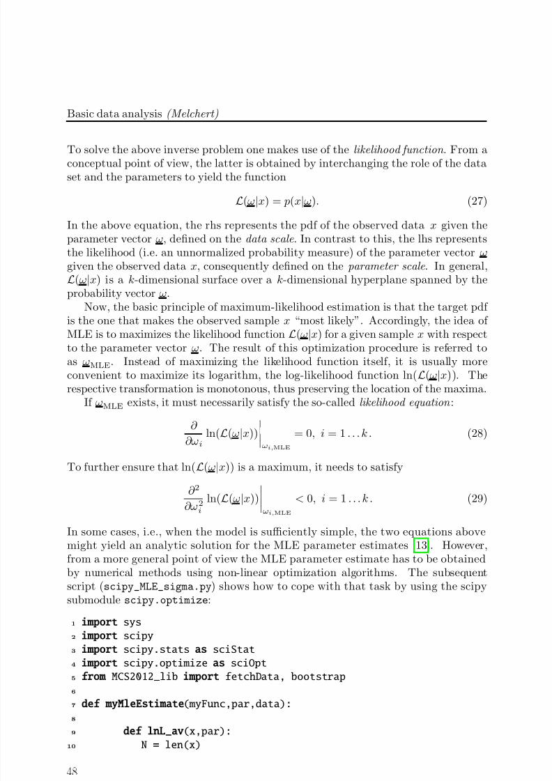
7/27/2019 Big Data Analysis using Python
http://slidepdf.com/reader/full/big-data-analysis-using-python 48/62
Basic data analysis (Melchert)
To solve the above inverse problem one makes use of the likelihood function . From aconceptual point of view, the latter is obtained by interchanging the role of the dataset and the parameters to yield the function
L(ω|x) = p(x|ω). (27)
In the above equation, the rhs represents the pdf of the observed data x given theparameter vector ω, defined on the data scale . In contrast to this, the lhs representsthe likelihood (i.e. an unnormalized probability measure) of the parameter vector ωgiven the observed data x, consequently defined on the parameter scale . In general,L(ω|x) is a k-dimensional surface over a k-dimensional hyperplane spanned by theprobability vector ω.
Now, the basic principle of maximum-likelihood estimation is that the target pdf is the one that makes the observed sample x “most likely”. Accordingly, the idea of MLE is to maximizes the likelihood function L(ω|x) for a given sample x with respectto the parameter vector ω. The result of this optimization procedure is referred toas ωMLE. Instead of maximizing the likelihood function itself, it is usually moreconvenient to maximize its logarithm, the log-likelihood function ln(L(ω|x)). Therespective transformation is monotonous, thus preserving the location of the maxima.
If ωMLE exists, it must necessarily satisfy the so-called likelihood equation :
∂
∂ωiln(L(ω|x))
ωi,MLE
= 0, i = 1 . . . k . (28)
To further ensure that ln(L(ω|x)) is a maximum, it needs to satisfy
∂ 2
∂ω2i
ln(L(ω|x))
ωi,MLE
< 0, i = 1 . . . k . (29)
In some cases, i.e., when the model is sufficiently simple, the two equations above
might yield an analytic solution for the MLE parameter estimates [13]. However,from a more general point of view the MLE parameter estimate has to be obtainedby numerical methods using non-linear optimization algorithms. The subsequentscript (scipy_MLE_sigma.py) shows how to cope with that task by using the scipysubmodule scipy.optimize:
1 import sys
2 import scipy
3 import scipy.stats as sciStat
4 import scipy.optimize as sciOpt
5 from MCS2012_lib import fetchData, bootstrap
6
7 def myMleEstimate(myFunc,par,data):
8
9 def lnL_av(x,par):
10 N = len(x)
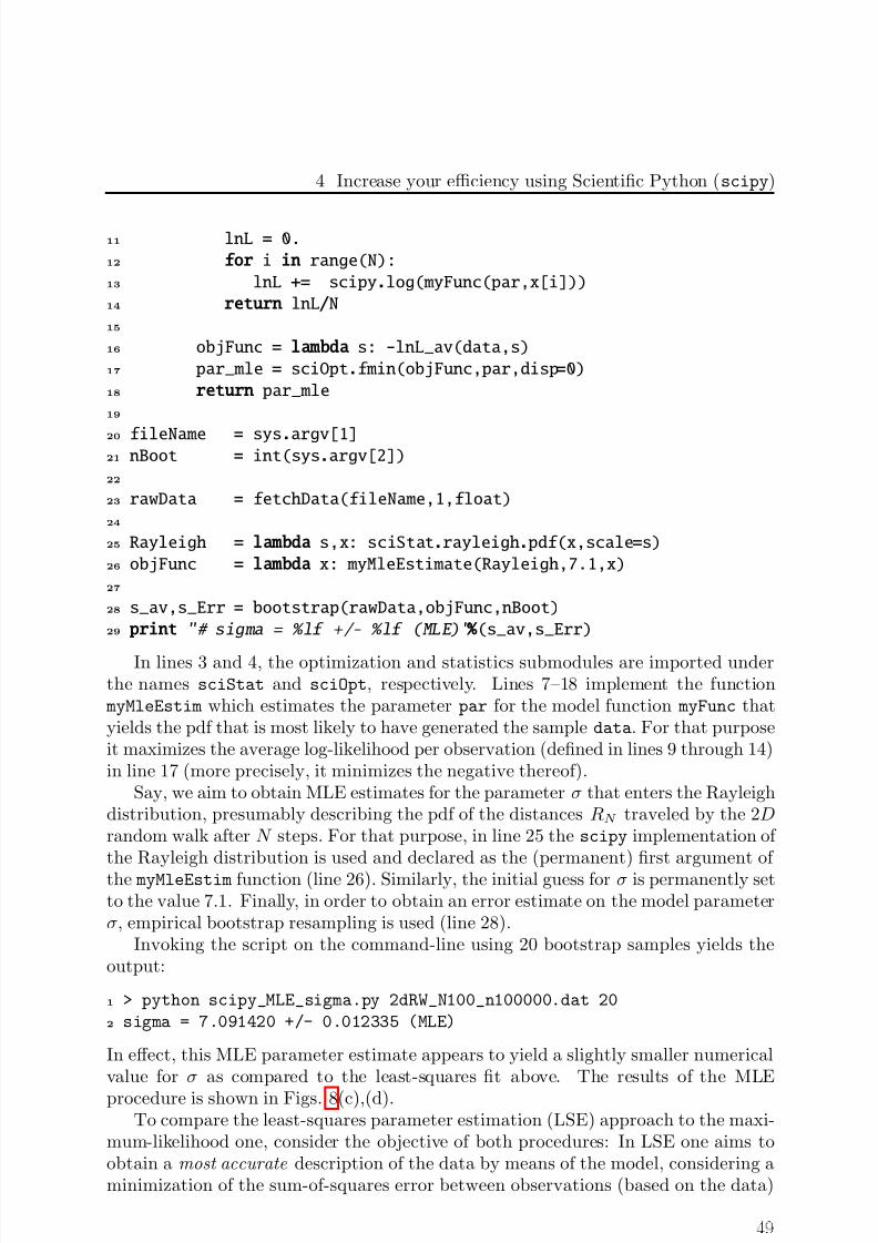
7/27/2019 Big Data Analysis using Python
http://slidepdf.com/reader/full/big-data-analysis-using-python 49/62
4 Increase your efficiency using Scientific Python (scipy)
11 lnL = 0.
12 for i in range(N):
13 lnL += scipy.log(myFunc(par,x[i]))
14 return lnL/N
15
16 objFunc = lambda s: -lnL_av(data,s)
17 par_mle = sciOpt.fmin(objFunc,par,disp=0)
18 return par_mle
19
20 fileName = sys.argv[1]21 nBoot = int(sys.argv[2])
22
23 rawData = fetchData(fileName,1,float)
24
25 Rayleigh = lambda s,x: sciStat.rayleigh.pdf(x,scale=s)
26 objFunc = lambda x: myMleEstimate(Rayleigh,7.1,x)
27
28 s_av,s_Err = bootstrap(rawData,objFunc,nBoot)
29 print "# sigma = %lf +/- %lf (MLE)" % (s_av,s_Err)
In lines 3 and 4, the optimization and statistics submodules are imported underthe names sciStat and sciOpt, respectively. Lines 7–18 implement the function
myMleEstim which estimates the parameter par for the model function myFunc thatyields the pdf that is most likely to have generated the sample data. For that purposeit maximizes the average log-likelihood per observation (defined in lines 9 through 14)in line 17 (more precisely, it minimizes the negative thereof).
Say, we aim to obtain MLE estimates for the parameter σ that enters the Rayleighdistribution, presumably describing the pdf of the distances RN traveled by the 2Drandom walk after N steps. For that purpose, in line 25 the scipy implementation of the Rayleigh distribution is used and declared as the (permanent) first argument of
the myMleEstim function (line 26). Similarly, the initial guess for σ is permanently setto the value 7.1. Finally, in order to obtain an error estimate on the model parameterσ, empirical bootstrap resampling is used (line 28).
Invoking the script on the command-line using 20 bootstrap samples yields theoutput:
1 > python scipy_MLE_sigma.py 2dRW_N100_n100000.dat 20
2 sigma = 7.091420 +/- 0.012335 (MLE)
In effect, this MLE parameter estimate appears to yield a slightly smaller numericalvalue for σ as compared to the least-squares fit above. The results of the MLE
procedure is shown in Figs. 8(c),(d).To compare the least-squares parameter estimation (LSE) approach to the maxi-
mum-likelihood one, consider the objective of both procedures: In LSE one aims toobtain a most accurate description of the data by means of the model, considering aminimization of the sum-of-squares error between observations (based on the data)
7/27/2019 Big Data Analysis using Python
http://slidepdf.com/reader/full/big-data-analysis-using-python 50/62
Basic data analysis (Melchert)
0
0.02
0.04
0.06
0.08
0.1
0 10 20 30
p ( R N
)
R N
(a)LSE
-3.2
-3.1
-3.0
-2.9
5 7 9 11
l n ( L ( σ ) ) / n
σ
(c)MLE
0
10
20
30
40
7.05 7.09 7.13
p ( σ M L E
)
σMLE
(d)MLE
0
10
20
30
7.08 7.13 7.18
p ( σ L S E )
σLSE
(b)LSE
Figure 8: Results of the least-squares and maximum-likelihood parameter estima-tion approaches. (a) Approximate pdf for the distance to the starting point (using30 bins), estimated from n = 105 2D random walks after N = 100 steps (datapoints) together with the most accurate fit to a Rayleigh distribution function ob-tained by a least-squares fit (solid line). (b) Approximate pdf (histogram using 16bins) of the resampled parameter σ as result of the bootstrap resampling procedure(1000 auxiliary data sets). The non-filled square indicates the result σ = 7.131(13).(c) Log-likelihood function as function of the single parameter σ. As evident fromthe figure, the maximum is approximately located at σ = 7.09. (d) Approximatepdf (histogram using 16 bins) of the resampled parameter σMLE as result of thebootstrap resampling procedure (1000 auxiliary data sets). The non-filled squareindicates the result σ = 7.091(11).
7/27/2019 Big Data Analysis using Python
http://slidepdf.com/reader/full/big-data-analysis-using-python 51/62
4 Increase your efficiency using Scientific Python (scipy)
and expectations (based on the model). In MLE, one aims at those parameters thatmaximize the log-likelihood and consequently yield those parameters that have most likely generated the data. Generally, MLE and LSE estimates differ from each other.In any case, a MLE estimate should be preferred over an LSE estimate. Finally,note that for statistically independent observations that are normally distributed,the maximization of the log-likelihood is equivalent to a minimization of the sum-of-squares error function.
4.4 Hierarchical cluster analysis using scipy
A cluster analysis might be used to classify a given set of “objects” with regard totheir “distance”. Therein, the measure of distance between either two objects can bequite general (not necessarily metric). E.g., below we will run a cluster analysis ona set of 6 points located in a 2D plane, wherein the euclidean distance between twopoints is used to measure their distance (in this particular example the objects arevector-valued observations and the distance measure is metric).
In order to perform a cluster analysis, many different algorithmic schemes are avail-able. Here we will illustrate one particular algorithm, falling into the realm of agglom-erative clustering methods, that generates a hierarchical clustering for a supplied dis-
tance matrix [15]. The respective algorithm assembles a hierarchical cluster startingfrom single-object clusters and can be found in the cluster submodule of scipy. Theparticular function we will use here is called scipy.cluster.hierarchy.linkage.The subsequent script (scipy_clusterAnalysis_cophDist.py) comprises a basic ex-ample that illustrates the usage of the above function:
1 import sys
2 import scipy
3 import scipy.cluster.hierarchy as sch
4 import scipy.spatial.distance as ssd
5 from dumpDendrogram import droPyt_distMat_dendrogram_sciPy
6
7 def myDistMatrix_2D(N,s):
8 scipy.random .seed(s)
9 xVec = scipy.rand(N,2)
10 Dij = scipy.zeros((N,N),dtype=’d ’)
11 for i in range(N):
12 for j in range(N):
13 Dij[i,j] = ssd.euclidean(xVec[i],xVec[j])
14 return Dij
15
16 def main():
17 # construct distance matrix
18 N = 6
19 Dij_sq = myDistMatrix_2D(N,0)
20
7/27/2019 Big Data Analysis using Python
http://slidepdf.com/reader/full/big-data-analysis-using-python 52/62
Basic data analysis (Melchert)
21 # obtain hierarchical clustering via scipy
22 Dij_cd = ssd.squareform(Dij_sq)
23 clusterResult = sch.linkage(Dij_cd, method=’average’)
24 corr,Cij_cd = sch.cophenet(clusterResult,Dij_cd)
25 Cij_sq = ssd.squareform(Cij_cd)
26
27 # print dendrogram on top of cophenetic distance
28 # matrix to standard outstream
29 droPyt_distMat_dendrogram_sciPy(Cij_sq,clusterResult,N)
30
31 main()
In lines 3 and 4, two scipy submodules are imported that are useful in the con-text of cluster analysis. The first one, scipy.cluster, contains a further submod-ule, implementing a collection of functions for hierarchical clustering, referred to asscipy.cluster.hierarchy. It allows to compute distance matrices from vector-valued observations, to generate hierarchical clusters from distance matrices, and topost-process the results obtained therein. The module scipy.spatial implementsvarious data structures that facilitate “spatial” computations. In particular, its sub-module scipy.spatial.distance contains functions that allow, e.g., to computedistance matrices from observations, and it implements a bunch of different distancefunctions, measuring the distance between two vector-valued observations. However,first and foremost, it allows to convert full (i.e. square) distance matrices to condensed(i.e. upper triangular) ones and vice versa. This is important since most functionsin scipy.cluster operate on condensed distance matrices. In line 5, the python
module dumpDendrogram is imported. It implements several functions that allow todisplay the results of a hierarchical cluster analysis as scalable vector graphics (SVG).(Note that scipy also offers means to display clusters via Dendrograms. However,sometimes it is useful to implement things on your own to dive into the nitty-grittydetails and to arrive at a more deep understanding of the matter.)
In the main routine, comprising lines 16 through 29, a full distance matrix, stem-ming from N = 6 vector-valued observations in 2D, is computed (line 19). For thispurpose, the function myDistMatrix_2D, defined in lines 7 through 14, is called. Inline 13, this function makes use of the euclidean distance function, contained in thescipy.spatial.distance submodule (of course, one could have implemented thisoneself). However, please note the way the multidimensional scipy array Dij is de-fined (line 10) and indexed (line 13). This is special to scipy arrays and is supposedto provide a slightly faster access to the array elements. As mentioned above, mostscipy.cluster functions assume condensed distance matrices. For this reason, inline 22, the function scipy.spatial.squareform is used to convert the full to a
condensed distance matrix.In line 23, the scipy function linkage is used to generate a hierarchical clustering
from the condensed distance matrix. In principal, it takes three arguments, the firstof which is the condensed distance matrix. The second argument specifies the methodby which the clustering will be computed, affecting the way distances between clusters
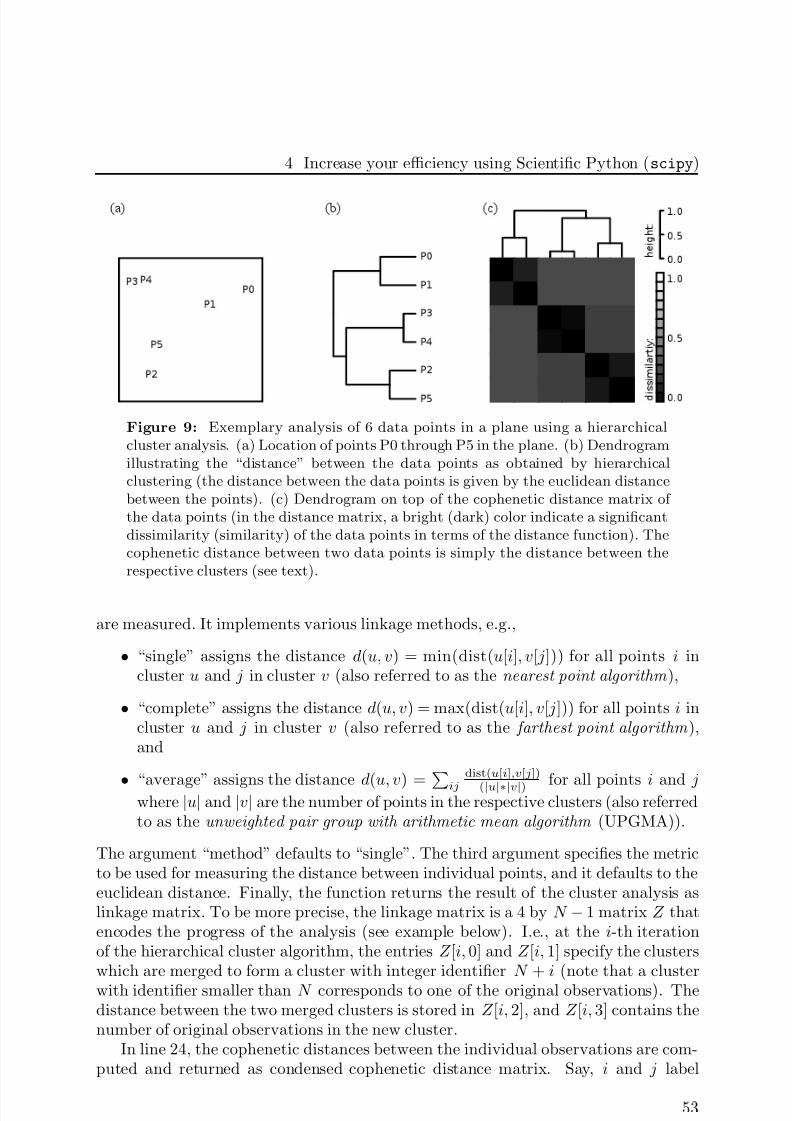
7/27/2019 Big Data Analysis using Python
http://slidepdf.com/reader/full/big-data-analysis-using-python 53/62
4 Increase your efficiency using Scientific Python (scipy)
Figure 9: Exemplary analysis of 6 data points in a plane using a hierarchicalcluster analysis. (a) Location of points P0 through P5 in the plane. (b) Dendrogramillustrating the “distance” between the data points as obtained by hierarchicalclustering (the distance between the data points is given by the euclidean distancebetween the points). (c) Dendrogram on top of the cophenetic distance matrix of the data points (in the distance matrix, a bright (dark) color indicate a significantdissimilarity (similarity) of the data points in terms of the distance function). Thecophenetic distance between two data points is simply the distance between therespective clusters (see text).
are measured. It implements various linkage methods, e.g.,
• “single” assigns the distance d(u, v) = min(dist(u[i], v[ j])) for all points i incluster u and j in cluster v (also referred to as the nearest point algorithm ),
• “complete” assigns the distance d(u, v) = max(dist(u[i], v[ j])) for all points i incluster u and j in cluster v (also referred to as the farthest point algorithm ),and
• “average” assigns the distance d(u, v) =
ij
dist(u[i],v[j])
(|u|∗|v|) for all points i and jwhere |u| and |v| are the number of points in the respective clusters (also referredto as the unweighted pair group with arithmetic mean algorithm (UPGMA)).
The argument “method” defaults to “single”. The third argument specifies the metricto be used for measuring the distance between individual points, and it defaults to theeuclidean distance. Finally, the function returns the result of the cluster analysis aslinkage matrix. To be more precise, the linkage matrix is a 4 by N − 1 matrix Z thatencodes the progress of the analysis (see example below). I.e., at the i-th iterationof the hierarchical cluster algorithm, the entries Z [i, 0] and Z [i, 1] specify the clusterswhich are merged to form a cluster with integer identifier N + i (note that a cluster
with identifier smaller than N corresponds to one of the original observations). Thedistance between the two merged clusters is stored in Z [i, 2], and Z [i, 3] contains thenumber of original observations in the new cluster.
In line 24, the cophenetic distances between the individual observations are com-puted and returned as condensed cophenetic distance matrix. Say, i and j label
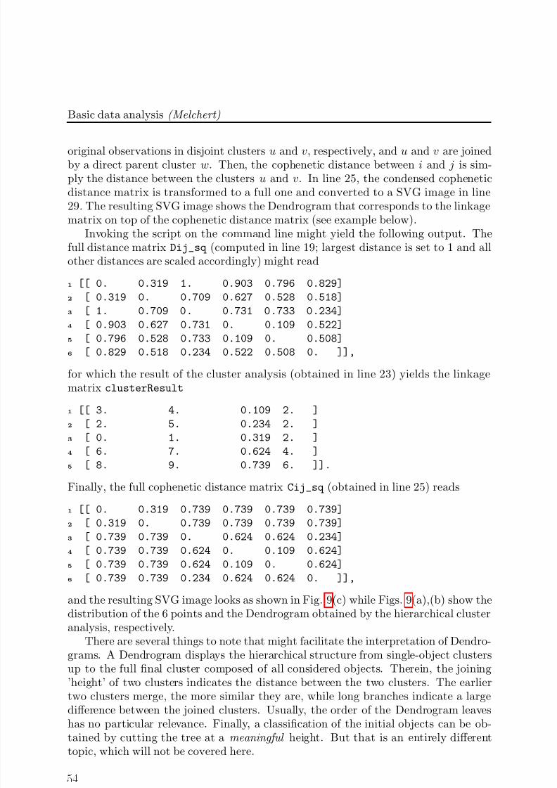
7/27/2019 Big Data Analysis using Python
http://slidepdf.com/reader/full/big-data-analysis-using-python 54/62
Basic data analysis (Melchert)
original observations in disjoint clusters u and v, respectively, and u and v are joinedby a direct parent cluster w. Then, the cophenetic distance between i and j is sim-ply the distance between the clusters u and v. In line 25, the condensed copheneticdistance matrix is transformed to a full one and converted to a SVG image in line29. The resulting SVG image shows the Dendrogram that corresponds to the linkagematrix on top of the cophenetic distance matrix (see example below).
Invoking the script on the command line might yield the following output. Thefull distance matrix Dij_sq (computed in line 19; largest distance is set to 1 and allother distances are scaled accordingly) might read
1 [[ 0. 0.319 1. 0.903 0.796 0.829]
2 [ 0.319 0. 0.709 0.627 0.528 0.518]
3 [ 1. 0.709 0. 0.731 0.733 0.234]
4 [ 0.903 0.627 0.731 0. 0.109 0.522]
5 [ 0.796 0.528 0.733 0.109 0. 0.508]
6 [ 0.829 0.518 0.234 0.522 0.508 0. ]],
for which the result of the cluster analysis (obtained in line 23) yields the linkagematrix clusterResult
1
[[ 3. 4. 0.109 2. ]2 [ 2. 5. 0.234 2. ]
3 [ 0. 1. 0.319 2. ]
4 [ 6. 7. 0.624 4. ]
5 [ 8. 9. 0.739 6. ]].
Finally, the full cophenetic distance matrix Cij_sq (obtained in line 25) reads
1 [[ 0. 0.319 0.739 0.739 0.739 0.739]
2 [ 0.319 0. 0.739 0.739 0.739 0.739]
3 [ 0.739 0.739 0. 0.624 0.624 0.234]
4 [ 0.739 0.739 0.624 0. 0.109 0.624]5 [ 0.739 0.739 0.624 0.109 0. 0.624]
6 [ 0.739 0.739 0.234 0.624 0.624 0. ]],
and the resulting SVG image looks as shown in Fig. 9(c) while Figs. 9(a),(b) show thedistribution of the 6 points and the Dendrogram obtained by the hierarchical clusteranalysis, respectively.
There are several things to note that might facilitate the interpretation of Dendro-grams. A Dendrogram displays the hierarchical structure from single-object clustersup to the full final cluster composed of all considered objects. Therein, the joining’height’ of two clusters indicates the distance between the two clusters. The earlier
two clusters merge, the more similar they are, while long branches indicate a largedifference between the joined clusters. Usually, the order of the Dendrogram leaveshas no particular relevance. Finally, a classification of the initial objects can be ob-tained by cutting the tree at a meaningful height. But that is an entirely differenttopic, which will not be covered here.
7/27/2019 Big Data Analysis using Python
http://slidepdf.com/reader/full/big-data-analysis-using-python 55/62
5 Struggling for speed
5 Struggling for speed
5.1 Combining C and python (Cython): sciencing as fast as youcan!
To reimplement the example in the following section, you will need to have the cython
extension module installed, see [9, 11].
As should be clear by now, code development in python is usually rather fastand the result is very concise and almost as readable as pseudocode. However, when
it comes to scientific computing and computationally rather involved tasks in dataanalysis (as e.g. bootstrap resampling), python scripts tend to be comparatively slow.One possible reason for this might be that the program spends lots of time in loopingconstructs which are costly in terms of computing time (using pure python). As aremedy one might use cython [9], an extension to the python language. It offers thepossibility to directly compile slightly modified python code to C, and to link theresulting C code against python. This yields compiled code that can be importedand executed by pure python scripts. In doing so, cython makes it possible to speedup python code and to directly interact with external C code.
In order to benefit from cython, there is no need to fully change your python
programming habits. This means that in a first step you can assemble your softwareproject as you would usually do in python, and in a second step you can identifythose parts that might be optimized further by means of cython. In this way you canselectively speed up your code where it is most beneficial.
To prepare pure python scripts for use with cython, you might amend the existingcode by statically declaring C data types for some variables using cython specific syn-tax. E.g., the cdef statement and the possibility to prepend data types in argumentlists are cython extensions to the original python language.
In effect, cython combines the speed of C with the flexibility and conciseness of python [11].
As an example to illustrate the extent to which an existing script needs to bealtered in order to achieve a valuable speed-up using cython, we will perform asmall benchmark test of python vs. cython. For this purpose, consider the followingpure python code (boxMueller_python.py) for the generation of Gaussian randomnumbers using the Box-M¨ uller method:
1 from math import pi,sqrt,log,sin
2 from random import seed,random
3
4 def gaussRand(mu,sigma):
5 u1 = random()
6 u2 = random()
7 r = sqrt(-2.*log(u1))
8 phi = 2.*pi*u2
9 return mu+sigma*r*sin(phi)
10
7/27/2019 Big Data Analysis using Python
http://slidepdf.com/reader/full/big-data-analysis-using-python 56/62
Basic data analysis (Melchert)
11 def main_python(N,mu,sigma):
12 seed(0)
13 for i in range(N):
14 z1 = gaussRand(mu,sigma)
In lines 1 and 2, several python functions from the math and random libraries areimported. Lines 4 through 9 define the function gaussRand() that uses two randomnumbers uniformly distributed in [0, 1) in order to generate one random deviate drawnfrom a Gaussian distribution with mean mu and width sigma. (Note: in principle, onecan generated two independent Gaussian random numbers by means of two indepen-dent uniformly distributed ones, but for the purpose of illustration let us just generateone of them.) Finally, lines 11 through 14 seed the random number generator andcall the above function N times using a looping construct.
A modified script for use with cython might look as the following code snippet(boxMueller_cython.pyx; cython scripts usually have the suffix .pyx):
1 cdef extern from "math.h" :
2 double sin(double)
3 double log(double)
4 double sqrt(double)
5 double M_PI6
7 cdef extern from "stdlib.h" :
8 double drand48()
9 void srand48(unsigned int SEED)
10
11 cdef double gaussRand(double mu,double sigma):
12 cdef double u1,u2,r,phi
13 u1 = drand48()
14 u2 = drand48()
15 r = sqrt(-2.*log(u1))16 phi = 2.*M_PI*u2
17 return mu+sigma*r*sin(phi)
18
19 def main_cython(N,mu,sigma):
20 cdef int i
21 srand48(0)
22 for i from 0<=i<N:
23 z = gaussRand(mu,sigma)
Therein, in lines 1 through 9, the same functions as in the pure python script are
imported. However, they are not imported from the “standard” python libraries butfrom the C header files math.h and stdlib.h. This illustrates the ability of cython
to directly interact with C code. In comparison to the python implementation, the Cimplementation of these functions are quite fast (since they lack the typical python
overheads spent by calling python functions). Regarding the function definition on
7/27/2019 Big Data Analysis using Python
http://slidepdf.com/reader/full/big-data-analysis-using-python 57/62
5 Struggling for speed
line 11, the return value of the gaussRand() function is declared as double, and itis defined via the cdef statement. The latter results in faster function calling viacython. Further, in the argument list of the function the data types of the variablesare prepended. More precisely, both arguments are declared to be of type double. Inthe block of statements that follows the function definition, the data types of all thevariables are declared which also results in a significant speed-up of the resulting Ccode. Note that in principle one can also mix declaration and value assignment, i.e.,statements such as cdef double phi = 2.*M_PI*u2 work very well. Finally, in line20 the data type of the index idx is declared to be of type int and in line 22 a faster
version of the for ... in range(...): statement, namely the for ... from ... :is implemented.
Post-processing of the resulting .pyx-cython script uses the setup script setup.py:
1 from distutils.core import setup
2 from distutils.extension import Extension
3 from Cython.Distutils import build_ext
4
5 setup(
6 cmdclass = ’build_ext’: build_ext,
7 ext_modules = [Extension("boxMueller_cython" ,\8 ["boxMueller_cython.pyx" ])],
9 )
Invoking the script by python setup.py build_ext --inplace yields the sharedlibrary boxMueller_cython.so, which you can import and use within any python
script. The above setup.py script uses the distutils module which provides supportfor building extension modules for python. Furthermore, it uses the Cython moduleto extend the capabilities of python.
Now, the benchmark test might be performed as follows: create a minimal python
script that executes the functions main_python and main_cython for the parametersN = 107, µ = 0., σ = 1., and determines the respective running times using thetimeit module [10] (timeit offers the possibility to time small pieces of python
code; as an alternative you might use the common unix tool time). This might lookas follows (benchmark_boxMueller.py):
1 from timeit import Timer
2
3 N=10000000
4
5 # time PYTHON code
6 t_py = Timer("main_python(%d,0.,1.)" % (N),
7 "from boxMueller_python import main_python"
8 ).timeit(number=1)
9
10 # time CYTHON code
7/27/2019 Big Data Analysis using Python
http://slidepdf.com/reader/full/big-data-analysis-using-python 58/62
Basic data analysis (Melchert)
11 t_cy = Timer("main_cython(%d,0.,1.)" % (N),
12 "from boxMueller_cython import main_cython"
13 ).timeit(number=1)
14
15 print "# PYTHON vs CYTHON: Box-Mueller Benchmark test"
16 print "# number of random deviates N=" ,N
17 print "# PYTHON: t_PY =" ,t_py
18 print "# CYTHON: t_CY =" ,t_cy
19 print "# speed-up factor t_PY/t_CY =" ,t_py/t_cy
Calling it on the command line yields:
1 > python benchmark_boxMueller.py
2 # PYTHON vs CYTHON: Box-Mueller Benchmark test
3 # number of random deviates N= 10000000
4 # PYTHON: t_PY = 10.7791149616
5 # CYTHON: t_CY = 0.316421031952
6 # speed-up factor t_PY/t_CY = 34.0657348063
Hence, the cython code outperforms the pure python code by a factor of approxi-
mately 34. Given the few changes that were necessary in order to generate the sharedlibrary boxMueller_cython.so, this is an impressive speed-up.
5.2 Parallel computing and python: do both!
Another way to speed up computations is to perform them in parallel, if possible.For this purpose, python offers several modules such as, e.g., the threading and
multiprocessing modules. However, if you want to benefit from the speed-up thatcan be achieved by using multiple cores simultaneously, you might want to go for thelatter one. The problem with the threading module is that it suffers from the “Global
Interpreter Lock” (GIT), which effectively limits the performance of the code sinceit allows only one thread at a time to execute python code. The multiprocessing
module does not suffer from a GIT and yields a speed-up that depends on the numberof cores that are available.
As an example to illustrate the multiprocessing module we here perform a paral-lel simulation of random walks. This is a rather simple application where subprocessesdo not need to communicate ( mp_2DrandWalk_oop.py):
1 from math import sqrt,cos,sin,pi
2 import random
3 import multiprocessing
4
5 class myProcess(multiprocessing.Process):
6 def __init__(self,myLock,myRng,mySeed,Nsteps):
7 self . myLock = myLock
8 self . myRng = myRng
7/27/2019 Big Data Analysis using Python
http://slidepdf.com/reader/full/big-data-analysis-using-python 59/62
5 Struggling for speed
9 self . mySeed = mySeed
10 self .Nsteps = Nsteps
11 multiprocessing.Process.__init__(self)
12
13 def run(self):
14 self . myRng.seed(self . mySeed)
15 x=y=0.
16 for i in range(self .Nsteps):
17 phi = self . myRng.random()*2.*pi
18 x += cos(phi)19 y += sin(phi)
20 self . myLock.acquire()
21 print self . mySeed,sqrt(x*x+y*y)
22 self . myLock.release()
23
24 def main():
25 N = 10000
26 nSamp = 5
27 myLock = multiprocessing.Lock()
28 for s in range(nSamp):29 myRng = random .Random()
30 process = myProcess(myLock,myRng,s,N)
31 process.start()
32
33 for p in multiprocessing.active_children():
34 print "random walk ID: " , p. mySeed
35
36 main()
The pivotal object, contained in the multiprocessing module, is the Process class.In lines 5–22 of the above example, we derived the subclass myProcess that overwritesthe default constructor of the Process class (lines 6–11) in order to generate an in-stance of the class that has several additional properties: myLock, a lock that preventsmultiple processes to write to the standard output simultaneously, myRng and mySeed,specifying its own instance of a random number generator and the respective seed,and Nstep, referring to the number of steps in the walk. The method run, definedin lines 13–22, finally implements the 2D random walk and prints the seed and thegeometric distance to the starting point to the standard output (thereby using thelock in order to make sure that the output is not messed up by other processes). In
line 31 of the function main, the start method of the Process class is called. Ineffect, the start method invokes the run method of the class and starts the activityof the process. All active processes can be addressed by a call to active_children,which returns a list of all active children of the current process. This is illustrated inlines 33 and 34. Finally, invoking the script on the command line yields the output:
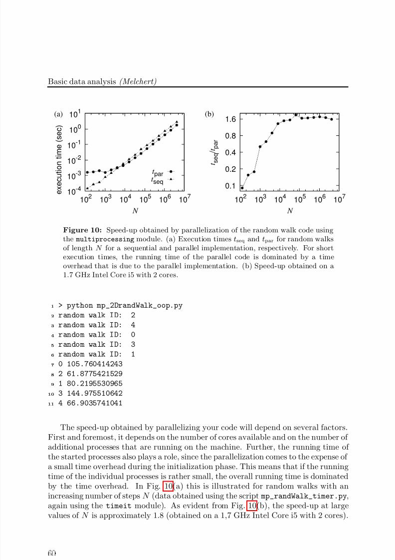
7/27/2019 Big Data Analysis using Python
http://slidepdf.com/reader/full/big-data-analysis-using-python 60/62
Basic data analysis (Melchert)
10-4
10-3
10-2
10-1
100
101
102 103 104 105 106 107 e x e c u t i o n t i m e ( s e c )
N
(a)
t part seq
0.1
0.2
0.4
0.8
1.6
102 103 104 105 106 107
t s e q
/ t p a r
N
(b)
Figure 10: Speed-up obtained by parallelization of the random walk code usingthe multiprocessing module. (a) Execution times tseq and tpar for random walksof length N for a sequential and parallel implementation, respectively. For shortexecution times, the running time of the parallel code is dominated by a timeoverhead that is due to the parallel implementation. (b) Speed-up obtained on a1.7 GHz Intel Core i5 with 2 cores.
1 > python mp_2DrandWalk_oop.py
2 random walk ID: 2
3 random walk ID: 4
4 random walk ID: 0
5 random walk ID: 3
6 random walk ID: 1
7 0 105.760414243
8 2 61.8775421529
9 1 80.2195530965
10 3 144.97551064211 4 66.9035741041
The speed-up obtained by parallelizing your code will depend on several factors.First and foremost, it depends on the number of cores available and on the number of additional processes that are running on the machine. Further, the running time of the started processes also plays a role, since the parallelization comes to the expense of a small time overhead during the initialization phase. This means that if the runningtime of the individual processes is rather small, the overall running time is dominatedby the time overhead. In Fig. 10(a) this is illustrated for random walks with anincreasing number of steps N (data obtained using the script mp_randWalk_timer.py,again using the timeit module). As evident from Fig. 10(b), the speed-up at largevalues of N is approximately 1.8 (obtained on a 1,7 GHz Intel Core i5 with 2 cores).
7/27/2019 Big Data Analysis using Python
http://slidepdf.com/reader/full/big-data-analysis-using-python 61/62
6 Further reading
6 Further reading
In the following I will list a selection of references wherein some more background (orsimply further useful information) on the topics covered in Section 2 can be found.
In order to prepare Section 2.1, I used Refs. [14] (see appendix C) and [17] (seechapter 7.1). In particular, the part on “Basic parameters related to random vari-ables” was prepared using Ref. [20] (see chapter 14.1). The part on “Estimatorswith(out) bias” picked up a little bit of stem from Ref. [12]. Section 2.2 was preparedusing Refs. [17] (see chapter 7.3.3) and [19]. The latter reference is a research article
with focus on analyzing power law distributed data. Section 2.3 on unbiased errorestimation via bootstrap resampling could benefit from Refs. [20] (see chapter 15.6)and [17] (see chapter 7.3.4). Also, Ref. [16] considers the bootstrap method in termsof an example problem (see problem 11.12), dealing with error estimation. Finally,Section 2.4 on the chi-square test was partly prepared using Refs. [20] (see chapter14.3), [17] (see chapter 7.5.1), and [12] (see chapter 4.6).
Acknowledgements. I would like to thank A. K. Hartmann, C. Norrenbrock, andP. Fieth for critically reading the manuscript and for providing comments and sug-gestions that helped to amend the document.
References
[1] The supplementary material can be downloaded from the site http://www.mcs.
uni-oldenburg.de/.
[2] A comprehensive python tutorial can be found at http://docs.python.org/
tutorial/.
[3] For more information on the Timsort algorithm, see http://en.wikipedia.org/
wiki/Timsort.[4] Python is a high-level general-purpose programming language that can be applied
to many different classes of problems, see http://www.python.org/.
[5] gnuplot is a command-line driven interactive data and function plotting utility,see http://www.gnuplot.info.
[6] For more information on the scipy package, see http://www.scipy.org/.
[7] Graphviz is an open source graph visualization software, see http://www.
graphviz.org/.
[8] Scipy Central is a code sharing and software list site focused on the scipy module,see http://scipy-central.org/item/36/2/.
[9] For more information on the cython extension to the python language, see http:
//www.cython.org/.
7/27/2019 Big Data Analysis using Python
http://slidepdf.com/reader/full/big-data-analysis-using-python 62/62
Basic data analysis (Melchert)
[10] For more information on the timeit module, see http://docs.python.org/
library/timeit.html.
[11] S. Behnel, R. Bradshaw, C. Citro, L. Dalcin, D. S. Seljebotn, and K. Smith.Cython: The best of both worlds. IEEE Comp. Sci. and Eng., 13:31–39, 2010.
[12] J. S. Bendat and A. G. Piersol. Random Data: Analysis and Measurement Procedures . Wiley-Interscience, New York, 1971.
[13] A. Clauset, C. R. Shalizi, and M. E. J. Newman. Power-law distributions in
empirical data. SIAM Rev., 51:661–703, 2007.
[14] T. H. Cormen, C. E. Leiserson, R. L. Rivest, and C. Stein. Introduction toAlgorithms, 2nd edition . MIT Press, 2001.
[15] G. Gan, C. Ma, and J. Wu. Data Clustering: Theory, Algorithms, and Applica-tions . ASA-SIAM, Philadelphia, 2007.
[16] H. Gould, J. Tobochnik, and W. Christian. An Introduction to Computer Simu-lation Methods . Addison Wesley, San Francisco, 2007.
[17] A. K. Hartmann. Practical Guide to Computer Simulations . World Scientific,Singapore, 2009.
[18] I. J. Myung. Tutorial on maximum likelihood estimation. J. Math. Psych.,47:90–100, 2003.
[19] M. E. J. Newman. Power laws, Pareto distributions and Zipf’s law. Contemporary Physics , 46:323–351, 2005.
[20] W. H. Press, S. A. Teukolsky, W. T. Vetterling, and B. P. Flannery. Numerical Recipes in C . Cambridge University Press, Cambridge, U.K., 1992.