Big-Alabo, Akuro (2015) Multilayered sensor -actuator ...theses.gla.ac.uk/6474/7/2015Big-Alabophd.pdf · Big-Alabo, Akuro (2015) Multilayered sensor -actuator plates for active mitigation

Glasgow Theses Service http://theses.gla.ac.uk/

[email protected]

n

Big-Alabo, Akuro (2015) Multilayered sensor-actuator plates for active mitigation of elastoplastic impact effects. PhD thesis. http://theses.gla.ac.uk/6474/ Copyright and moral rights for this thesis are retained by the author A copy can be downloaded for personal non-commercial research or study, without prior permission or charge This thesis cannot be reproduced or quoted extensively from without first obtaining permission in writing from the Author The content must not be changed in any way or sold commercially in any format or medium without the formal permission of the Author When referring to this work, full bibliographic details including the author, title, awarding institution and date of the thesis must be given

MULTILAYERED SENSOR-ACTUATOR PLATES

FOR ACTIVE MITIGATION OF ELASTOPLASTIC

IMPACT EFFECTS

by

Akuro Big-Alabo

THESIS SUBMITTED IN FULFILMENT OF THE REQUIREMENTS FOR THE

DEGREE OF DOCTOR OF PHILOSOPHY IN MECHANICAL ENGINEERING

SCHOOL OF ENGINEERING

COLLEGE OF SCIENCE AND ENGINEERING

UNIVERSITY OF GLASGOW

May 2015

ii

Abstract

Analytical models have been used here to conduct detailed studies on the

elastoplastic response of rectangular plates subjected to normal impact of a

rigid sphere. Analytical models have been derived using a complete modelling

approach in which the equations of motion of the contacting bodies (i.e. the

plate and spherical impactor) and a compliance law for the local contact

mechanics are used to formulate the impact model. To account for the local

contact mechanics, a novel Meyer-type compliance model based on elastic-

elastoplastic-fully plastic material behaviour has been formulated and validated

using published experimental results. This compliance model was used to

investigate the elastoplastic impact response of both transversely inflexible and

transversely flexible rectangular plates. Particular attention has been given to

solving the nonlinear impact models, leading to the development of a new

algorithm to solve the nonlinear models of a half-space impact. The algorithm is

simple, inherently stable and converges very quickly. For transversely flexible

plate impact, investigations were centred on the elastoplastic impact response

of a three-layer laminated plate structure called a trimorph plate. The

understanding gained from investigating the elastoplastic impact response of an

Al/PVDF/PZT trimorph plate was applied to study a newly proposed strategy for

active mitigation of elastoplastic impact effects i.e. plastic deformation and/or

damage. The idea behind the strategy was to use bonded piezoactuators to

actively induce a state of pre-stress in the host layer, which in turn influenced

the impact response of the plate. A preliminary qualitative analysis of the

proposed strategy was conducted using analytically derived models for a

PZT/Al/PZT trimorph plate and the results obtained showed that the proposed

strategy can be used to achieve significant levels of mitigation against

elastoplastic impact effects.

iii

Table of contents

Abstract....................................................................................... ii

Table of contents ........................................................................... iii

List of Tables ............................................................................... vii

List of Figures .............................................................................. viii

Acknowledgement ........................................................................ xiii

Author’s Declaration .......................................................................xiv

Nomenclature ............................................................................... xv

CHAPTER ONE ................................................................................. 1

INTRODUCTION ............................................................................... 1

1.1 Background .......................................................................... 1

1.2 Motivation ........................................................................... 3

1.3 Aims and objectives ............................................................... 4

1.4 Scope of study ...................................................................... 7

1.5 Contributions of study ............................................................. 8

1.6 Structure of thesis ............................................................... 10

CHAPTER TWO .............................................................................. 12

VIBRATION ANALYSIS OF MULTILAYERED PLATES ...................................... 12

Chapter summary ........................................................................ 12

2.1 Review of plate vibration modelling .......................................... 12

2.2 Classical plate theory ........................................................... 17

2.2.1 Assumptions used in formulating the rectangular plate vibration model

based on the CPT ..................................................................... 17

2.2.2 Transverse force analysis ..................................................... 18

2.2.3 In-plane force analysis ........................................................ 20

2.2.4 In-plane force effect on flexural oscillations .............................. 22

2.2.5 Strain-displacement relationships for CPT ................................. 24

iv

2.3 First-order shear deformation plate theory.................................. 25

2.3.1 Strain-displacement relationships for FSDPT .............................. 27

2.3.2 Rectangular plate vibration model based on FSDPT ...................... 28

2.4 Constitutive equations of laminated rectangular plates ................... 29

2.4.1 Constitutive equations for a thin rectangular laminate based on CPT 31

2.4.2 Constitutive equations for a moderately thick rectangular laminate

based on FSDPT ........................................................................ 32

2.5 Determination of the laminate stiffness coefficients ...................... 33

2.6 Vibration analysis of a trimorph plate ........................................ 35

2.6.1 Vibration analysis of a thin trimorph plate ................................ 36

2.6.2 Vibration analysis of a moderately thick trimorph plate ................ 46

2.7 Chapter conclusions ............................................................. 49

CHAPTER THREE ............................................................................ 51

CONTACT MODEL FOR ELASTOPLASTIC INDENTATION ................................ 51

Chapter summary ........................................................................ 51

3.1 Review of contact models for spherical indentation of elastoplastic half-

space ...................................................................................... 51

3.1.1 Contact models for post-yield indentation of a metallic half-space ... 53

3.1.2 Contact models for post-yield indentation of a transversely isotropic

half-space .............................................................................. 61

3.2 New contact model for post-yield indentation of a half-space by a

spherical indenter ....................................................................... 64

3.2.1 Determination of contact parameters of the new contact model...... 68

3.2.2 Normalised form of new contact model .................................... 73

3.3 Validation of new contact model .............................................. 74

3.3.1 Some observations of the new contact model............................. 74

3.3.2 Static indentation analysis ................................................... 76

3.3.3 Dynamic indentation analysis ................................................ 82

3.4 Chapter conclusions ............................................................. 92

v

CHAPTER FOUR ............................................................................. 94

IMPACT ANALYSIS OF RECTANGULAR PLATES SUBJECTED TO NORMAL IMPACT OF A

RIGID SPHERICAL IMPACTOR .............................................................. 94

Chapter summary ........................................................................ 94

4.1 Review of analytical models for rigid object impact on compliant targets

...................................................................................... 94

4.1.1 The spring-mass model ....................................................... 100

4.1.2 The energy-balance model .................................................. 101

4.1.3 The infinite plate model ..................................................... 102

4.1.4 The complete model ......................................................... 103

4.2 Elastoplastic impact response analysis of transversely inflexible

rectangular plates ...................................................................... 105

4.3 Algorithm for the solution of the impact model of transversely inflexible

rectangular plates ...................................................................... 112

4.3.1 Concept of the FILM .......................................................... 114

4.3.2 Solution of half-space impact modelled based on a canonical

compliance law using the FILM .................................................... 116

4.3.3 Solution of half-space impact modelled based on a non-canonical

compliance law using the FILM .................................................... 121

4.3.4 Implications of applying the FILM approach for the solution of the

impact response of transversely flexible plates ................................. 124

4.4 Impact response of transversely flexible rectangular plates ............. 131

4.4.1 Validation of modelling and solution approach .......................... 134

4.4.2 Elastoplastic impact response analysis of a transversely flexible

trimorph plate ........................................................................ 135

4.5 Chapter conclusions ............................................................ 151

CHAPTER FIVE ............................................................................. 153

MITIGATION OF ELASTOPLATIC IMPACT EFFECTS USING PIEZOACTUATORS ...... 153

Chapter summary ....................................................................... 153

5.1 Review of impact damage of transversely flexible plates ................ 153

vi

5.2 Impact damage mitigation ..................................................... 156

5.2.1 Passive mitigation of impact damage ...................................... 156

5.2.2 Active mitigation of impact damage ....................................... 158

5.3 Piezoelectric actuation effect ................................................ 160

5.4 Active mitigation of elastoplastic impact effects using piezoactuators 164

5.4.1 Analytical models for investigating impact damage mitigation using

active piezoelectric pre-stressing ................................................. 165

5.4.2 Results and discussions on mitigation of elastoplastic impact effects

using PZT/Al/PZT plate ............................................................. 169

5.5 Implementation issues of the proposed strategy for active impact

damage mitigation ..................................................................... 176

5.6 Chapter conclusions ............................................................ 178

CHAPTER SIX ............................................................................... 179

CONCLUSIONS AND RECOMMENDATIONS ............................................... 179

6.1 Conclusions of thesis ........................................................... 179

6.2 Recommendations for future research ...................................... 182

APPENDICES ................................................................................ 185

Appendix A.1: Algebra in the derivation of the cubic equation for 𝛿𝑡𝑒𝑝 ....... 185

Appendix A.2: Deformation work during contact loading ........................ 186

Appendix B.1: Mathematica code to implement FILM algorithm for solution of

half-space impact ...................................................................... 188

Appendix B.2: Mathematica code to implement FILM algorithm for infinite

plate impact ............................................................................. 190

Appendix B.3: Mathematica code to solve the impact model of the trimorph

plate ...................................................................................... 192

REFERENCES ................................................................................ 202

vii

List of Tables

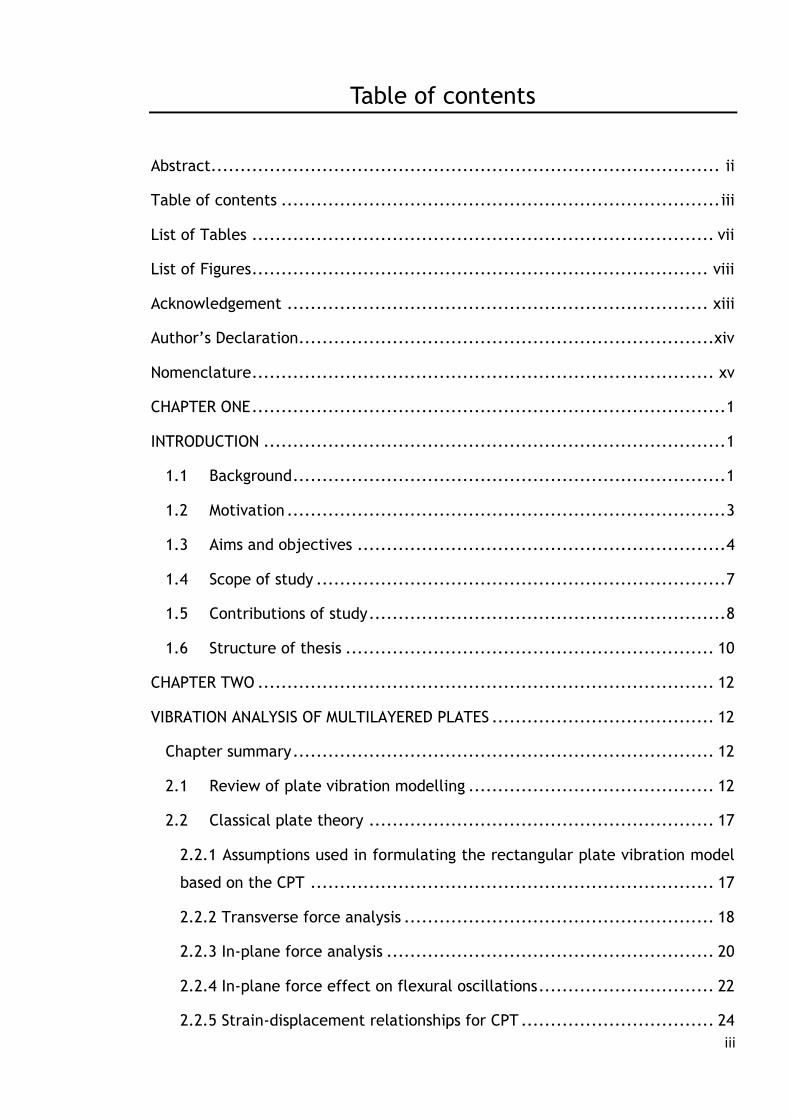
Table 2.1: Material properties of the trimorph plate layers ...................... 38

Table 2.2: Response characteristics for small flexural oscillations 𝜇 = 0.05.... 40

Table 2.3: Response characteristics for large flexural oscillations 𝜇 = 0.001 .. 40

Table 2.4: Modal frequencies and responses of a moderately thick Al/PVDF/PZT

plate during small flexural oscillations ................................................ 48

Table 3.1: Material properties for indentation of pure Nickel by spherical 10%

Cobalt-Tungsten Carbide Indenter (Brake, 2012)..................................... 78

Table 3.2: Material properties for indentation of AISI 1035 Steel by spherical

Tungsten Carbide Indenter (Brake, 2012) .............................................. 80

Table 3.3: Material properties for experiments by Kharaz and Gorham (2000) 89

Table 3.4: Material properties for experiments by Mok and Duffy (1965) ...... 91

Table 4.1: Legend for impact response of transversely inflexible plate ........ 108

Table 4.2: Results of the impact response of steel ................................. 112

Table 4.3: Tungsten carbide – mild steel impact response results obtained using

FILM ......................................................................................... 124

Table 4.4: Properties of the steel –laminate impact system (Olsson, 1992) ... 127

Table 4.5: Material and geometrical properties of the layers of the trimorph

plate ........................................................................................ 139

Table 5.1: Modal dependence of mechanical and piezoelectric stiffnesses .... 173

Table 5.2: Effect of actively induced pre-stress on critical impact parameters

............................................................................................... 174

viii

List of Figures

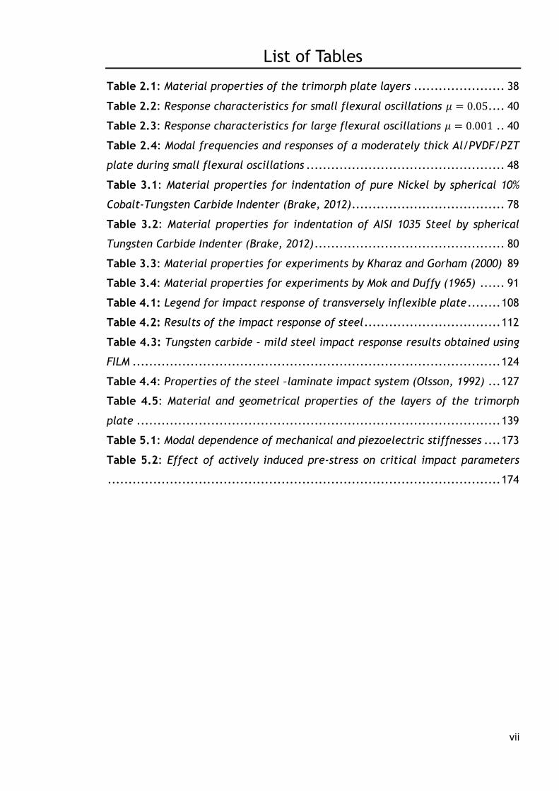
Figure 2.1: Plate element showing rectilinear coordinate system ................ 18

Figure 2.2: Lateral forces acting on the mid-plane ................................. 19

Figure 2.3: Bending moments acting on the mid-plane ............................. 19

Figure 2.4: In-plane forces acting on a rectangular plate element ............... 21

Figure 2.5: Effect of membrane forces on lateral deflection of plate ........... 22

Figure 2.6: Sketch illustrating vertical geometry of laminate .................... 30

Figure 2.7: Diagrammatic description of the excited system ...................... 35

Figure 2.8: Frequency-response of a thin trimorph plate during small flexural

oscillations of the plate centre 𝜇 = 0.05. ............................................. 41

Figure 2.9: Frequency-response of a thin trimorph plate during large flexural

oscillations of the plate centre 𝜇 = 0.001. ............................................ 42

Figure 2.10: Effect of nonlinear terms on the frequency-response of a thin

trimorph plate undergoing large flexural oscillations μ = 0.001. ................. 44

Figure 2.11a: Transient response of a thin Al/PVDF/PZT plate during small

flexural oscillations when excited at the undamped natural frequency. ........ 44

Figure 2.11b: Steady-state response of a thin Al/PVDF/PZT plate during small


Figure 2.12a: Complete response of a thin Al/PVDF/PZT plate during large


Figure 2.12b: Steady-state response of a thin Al/PVDF/PZT plate during large


Figure 2.13a: Transient response of a moderately thick Al/PVDF/PZT plate

during small flexural oscillations when excited at the undamped natural

frequency. .................................................................................. 49

Figure 2.13b: Steady-state response of a moderately thick Al/PVDF/PZT plate


frequency. .................................................................................. 49

Figure 3.1: Elastoplastic half-space impact of a rigid spherical indenter on a

compliant flat target (a) before impact (b) during impact (c) after impact. ... 52

Figure 3.2: Elastoplastic deformation at (a) yield (b) the onset of fully plastic

loading regime. The cross-hatched area is the surrounding elastically-deformed

material while the unshaded area is the plastically-deformed material. ....... 53

Figure 3.3: Sketch of compliance curve for the new contact law. ................ 65

ix

Figure 3.4: Plastic deformation in the elastoplastic loading regime (a) during

nonlinear elastoplastic deformation (b) during linear elastoplastic deformation.

The cross-hatched area is the surrounding elastically-deformed material while

the unshaded area is the plastically-deformed material. .......................... 66

Figure 3.5: Compliance curve for indentation of two identical SUJ2 Steel balls.

Present model – Solid line, Brake’s model – Dash line, Hertz model – Dot dash

line. .......................................................................................... 77

Figure 3.6: Compliance curve for indentation of pure Nickel. The maximum

indentation is well into the fully plastic regime. 𝛿𝑝 = 82.5; 𝛿𝑡𝑒𝑝 = 13.93 for the

present model. ............................................................................. 79


indentation is well into the fully plastic regime. 𝛿𝑝 = 30; 𝛿𝑡𝑒𝑝 = 20.6 for the

present model. ............................................................................. 79

Figure 3.8: Compliance curve for indentation of AISI 1035 Steel. The maximum

indentation is well into the fully plastic regime. 𝛿𝑝 = 82.5; 𝛿𝑡𝑒𝑝 = 13.93 for the

present model. ............................................................................. 81

Figure 3.9: Comparison of elastoplastic loading regime of present model with

the models of Brake (2012) and Majeed et al (2012) for indentation of AISI 1035

Steel. ........................................................................................ 82

Figure 3.10: Method to determine the maximum indentation and force during

impact. ...................................................................................... 87

Figure 3.11: Validation of analytical method for calculating the impactor

velocity profile during half-space impact. ............................................ 88

Figure 3.12: Coefficient of restitution for impact of aluminium oxide sphere on

AISI 1055 steel alloy slab. ................................................................ 90


aluminium T2014-T4 alloy slab. ......................................................... 90

Figure 3.14: Coefficient of restitution for impact of steel ball on Al 6061 and

steel C1018 alloy slabs. ................................................................... 91

Figure 4.1: Characteristics and solution methods for different impact

classifications. ............................................................................. 99

Figure 4.2: Spring-mass models (a) Complete 2-DOF (b) SDOF for quasi-static

impact (c) SDOF for half-space impact. ............................................... 100

Figure 4.3: Method for selection of impact model. ................................ 104

x

Figure 4.4: Impact response of a steel slab dynamically loaded by a tungsten

carbide ball into the nonlinear elastoplastic stage; 𝑉0 = 0.5 [𝑚/𝑠]. ............. 108

Figure 4.5a: Impact response of a steel slab dynamically loaded by a tungsten

carbide ball into the linear elastoplastic stage; 𝑉0 = 5.0 [𝑚/𝑠]. ................. 109

Figure 4.5b: Initial impact response of a steel slab dynamically loaded by a

tungsten carbide ball showing the elastic stage; 𝑉0 = 5.0 [𝑚/𝑠]. ................. 109

Figure 4.6: Energy evolution during impact of tungsten carbide ball on a mild

steel slab for 𝑉0 = 0.5 [𝑚/𝑠]. Kinetic energy: dash-dot line; Work done: short-

dash line. ................................................................................... 110


steel for 𝑉0 = 5[𝑚/𝑠]. Kinetic energy: dash-dot line; Work done: short-dash line.

............................................................................................... 111

Figure 4.8: Coefficient of restitution for impact of tungsten carbide ball on a

mild steel slab. ............................................................................ 111

Figure 4.9: Linear discretisation of nonlinear force indentation relationship (a)

one line (b) two lines (c) three lines. ................................................. 115

Figure 4.10: Tri-linear approximation of a general nonlinear impact force used

to demonstrate the concept of the FILM.............................................. 116

Figure 4.11: Comparison of the results of the FILM solution and numerical

integration method. Lines – FILM solution; Markers – numerical solution. See

Table 4.1 for line colour definition. ................................................... 121


integration method. Lines – FILM solution; Markers – numerical solution. Contact

model used: Stronge (2000a). See Table 4.1 for colours used in plotting the FILM

results. ..................................................................................... 123


integration method for elastic impact of [0/90/0/90/0]s graphite/epoxy

(T300/934) composite plate. Lines – FILM solution; Markers – numerical solution.

............................................................................................... 130

Figure 4.14a: Force and velocity histories for impact of a steel ball on a

transversely flexible steel plate. dW1/dt – plate velocity, dW2/dt – impactor

velocity, F – Force. ....................................................................... 135

Figure 4.14b: Displacement histories for impact of a steel ball on a transversely

flexible steel plate.W1 – plate displacement, W2 – impactor displacement. ... 135

xi

Figure 4.15: Effect of number of modes used in the solution of the impact

model on the accuracy of the results obtained for the Al/PVDF/PZT plate. ... 140

Figure 4.16: Displacement histories of Al/PVDF/PZT plate impacted by steel

impactor. Dotted line – impactor disp., short-dash line – plate disp., solid line –

indentation. ............................................................................... 140

Figure 4.17: Velocity histories of Al/PVDF/PZT plate struck by steel impactor.

Dotted line – impactor velocity, short-dash line – plate velocity, solid line –

relative velocity........................................................................... 141

Figure 4.18: Force history of Al/PVDF/PZT plate struck by steel impactor with

initial impact speed of 2.0 [m/s]. ..................................................... 142

Figure 4.19: Indentation history of Al/PVDF/PZT plate struck by steel impactor

with initial impact speed of 2.0 [m/s]. ............................................... 143

Figure 4.20a: Plate displacement during impact of Al/PVDF/PZT plate based on

CLPT and FSDPT. .......................................................................... 144

Figure 4.20b: Indentation response during impact of Al/PVDF/PZT plate based

on CLPT and FSDPT. ...................................................................... 144

Figure 4.20c: Force response during impact of Al/PVDF/PZT plate based on

CLPT and FSDPT. .......................................................................... 145

Figure 4.21: Effect of impactor mass on the impact response of Al/PVDF/PZT

plate. ....................................................................................... 146

Figure 4.22: Effect of impactor size on the impact response of Al/PVDF/PZT

plate. ....................................................................................... 146

Figure 4.23: Effect of impact velocity on the impact response of Al/PVDF/PZT

plate. ....................................................................................... 147

Figure 4.24: Effect of thickness on the impact response of Al/PVDF/PZT plate.

............................................................................................... 147

Figure 4.25: Effect of aspect ratio on the impact response of Al/PVDF/PZT

plate. ....................................................................................... 148

Figure 4.26: Impact response of Al/PVDF/PZT plate for the same impact energy

and different impact mass and velocity. ............................................. 149

Figure 4.27: Influence of apparent flexibility on the impact response of

Al/PVDF/PZT plate. ...................................................................... 150

Figure 5.1: Piezoelectric sheet poled along the 3-direction and having planar

surface covered with electrode. ....................................................... 162

xii

Figure 5.2: Symmetric PZT/Al/PZT laminate with PZT layers pole in the 3 –

direction. ................................................................................... 166

Figure 5.3: Free body diagram during activation of 𝑑31 stiffness coefficient of a

symmetric PZT/Al/PZT laminate. (a) Voltage and poling direction in-phase; (b)

voltage and poling direction are 180° out-of-phase. 𝐹𝑅 is the reactive force

transferred to the host layer and 𝐹𝑖 is the induced force in the piezoelectric

layer due to applied voltage. ........................................................... 168

Figure 5.4: Low-velocity impact response of PZT/Al/PZT with no induced pre-

stress. Blue line – plate response; red line – impactor response. ................. 171

Figure 5.5: Low-velocity impact response of PZT/Al/PZT with induced tensile

pre-stress. Blue line – plate response; red line – impactor response............. 171

Figure 5.6: Low-velocity impact response of PZT/Al/PZT with induced

compressive pre-stress. Blue line – plate response; red line – impactor response.

............................................................................................... 172

xiii

Acknowledgement

First and foremost, I wish to acknowledge the guidance of Almighty God in

my research and the opportunity that He availed me to undertake a PhD

research at this time.

I am very grateful to my supervisor, Dr. Philip Harrison, for the support and

advice he gave. In particular, I appreciate the fact that he accepted to supervise

me when there was a need to change my supervisor after my first year. Also, I

wish to express my profound gratitude to my second supervisor, Professor

Matthew P. Cartmell (from University of Sheffield), for his continued support,

encouragement and advice throughout my research.

To Pastor Chima Dioka and members of the Deeper Christian Life Ministry

(DCLM) Glasgow, you made my stay and life in Glasgow complete through the

warm fellowship we shared all the time. I pray that God will increase your

ministry, and that your message and charity will impact many more lives.

I would like to acknowledge the support of the administrative staff in the

School of Engineering, especially Elaine McNamara. To all friends and colleagues

at the University of Glasgow, I thank you for the good times we shared and the

encouragement we received from one another by sharing our experiences.

To my brothers, Adokiye, Tamunopubo, Sotonye and Miebaka, and my

mum, Mrs Kate Big-Alabo, thank you for helping me take care of my

responsibilities in Nigeria while I was in Glasgow for my research. Lastly, but not

the least, I would like to appreciate my loving wife, Mrs Ameze Big-Alabo, and

my cherished daughter, Miss Boma Big-Alabo. Both of you brought an invaluable

meaning to my life, and helped me to carry on during the most challenging

stages of my research.

Finally, the financial support of the Commonwealth Scholarship Commission

(CSC) United Kingdom, in the form of a full PhD Scholarship (CSC Award

Reference: NGCA-2011-60) is gratefully acknowledged.

xiv

Author’s Declaration

The work presented in this thesis is the original work of the author

undertaken at the University of Glasgow. The copyright of the material in this

thesis belongs to the author. Therefore, the author’s permission should be

obtained if any part of this thesis is to be reproduced in any form. However,

where ideas and conclusions from this thesis are referred to in any academic

endeavour, it is expected that the author would be properly acknowledged.

© A. Big-Alabo

2015

xv

Nomenclature

Abbreviations

CLPT Classical Laminate Plate Theory

CPT Classical Plate Theory

ESL Equivalent Single Layer

FE Finite Element

FEA Finite Element Analysis

FILM Force-Indentation Linearisation Method

FSDPT First-order Shear Deformation Plate Theory

HSDPT Higher-order Shear Deformation Plate Theory

MPT Mindlin Plate Theory

ODE Ordinary Differential Equation

PDE Partial Differential Equation

PDEx Partial Differential Expression

PVDF Polyvinylidene Flouride

PZT Lead Zirconate Titanate

RPT Reissner Plate Theory

RTSDPT Reddy Third-order Shear Deformation Plate Theory

Symbols

𝑎 Length of plate in x-direction; contact radius

𝑎 𝑥 ; 𝑎 𝑦 ; 𝑎 𝑧 Acceleration of plate in x-, y- and z-directions respectively

𝑎𝑦 Contact radius at yield point

𝑏 Length of plate in y-direction

𝑐 Damping coefficient per unit area

𝑑𝑖𝑗 Piezoelectric stiffness coefficient; 𝑖, 𝑗 = 1, 2, 3, 4, 5

𝑒 Coefficient of restitution

𝑕 Total thickness of plate

𝑘𝑥0 Curvature of the mid-plane of the plate about x-direction

𝑘𝑥𝑦0 Curvature of the mid-plane of the plate about x-y plane

𝑘𝑦0 Curvature of the mid-plane of the plate about y-direction

𝑚 Modal number in x-direction

𝑚𝑖 Mass of impactor

𝑚𝑝 Mass of plate

𝑛 Modal number in y-direction; number of discretisations in the FILM

xvi

𝑞(𝑥,𝑦, 𝑡) Spatially distributed excitation

𝑢; 𝑢(𝑥,𝑦, 𝑧, 𝑡) Displacement of plate in x-direction

𝑣; 𝑣(𝑥, 𝑦, 𝑧, 𝑡) Displacement of plate in y-direction

𝑤(𝑡) Transverse displacement of plate in infinite plate impact model

𝑤; 𝑤(𝑥,𝑦, 𝑡) Transverse displacement of plate

𝑤𝑖(𝑡) Displacement of impact in infinite plate impact model

𝑥𝑖 Displacement of impactor in spring-mass impact model

𝑥𝑝 Displacement of plate in spring-mass impact model

𝐴𝑖𝑗 Extensional stiffness elements

𝐵𝑖𝑗 Bending-extension stiffness elements

𝐷 Effective bending stiffness of an infinite plate

𝐷𝑖𝑗 Bending stiffness elements

𝐸 Young’s modulus

𝐸 Effective contact modulus

𝐹 Contact force

𝐹𝑒 Contact force during elastic loading

𝐹𝑒𝑝𝐼 Contact force during nonlinear elastoplastic loading

𝐹𝑒𝑝𝐼𝐼 Contact force during linear elastoplastic loading

𝐹𝑓𝑝 Contact force during fully plastic loading

𝐹𝑚 Maximum contact force

𝐹𝑝 Contact force at onset of fully plastic loading

𝐹𝑟𝑠 Linearised impact force for discretisation between points 𝑟 and 𝑠

𝐹𝑡𝑒𝑝 Contact force at transition point in the elastoplastic loading regime

𝐹𝑢 Contact force during unloading

𝐹𝑦 Contact force at yield point

𝐾 Mechanical bending stiffness per unit mass in complete impact model

𝐾𝑕 Hertz contact stiffness

𝐾𝑏 Bending stiffness of plate in spring-mass impact model

𝐾𝑐 Contact stiffness

𝐾𝑒𝑓𝑓 Effective bending stiffness of plate in the presence of induced pre-stress

𝐾𝑙 Linear contact stiffness during elastoplastic loading

𝐾𝑚 Membrane stiffness of plate in spring-mass impact model

𝐾𝑝 Linear contact stiffness during fully plastic loading

𝐾𝑟𝑠 Linearised contact stiffness for discretisation between points 𝑟 and 𝑠

𝐾𝑠 Shear stiffness of plate in spring-mass impact model

𝐾𝑢 Nonlinear contact stiffness during unloading

xvii

𝐿 Characteristic length of plate

𝑀𝑥 ; 𝑀𝑥𝑥 Moment about x-axis

𝑀𝑥𝑦 Moment about x-y plane

𝑀𝑦 ; 𝑀𝑦𝑦 Moment about y-axis

𝑁 Total number of layers in laminate plate

𝑁𝑎 Number of actuated layers

𝑁𝑥 ; 𝑁𝑥𝑥 Membrane or in-plane force per unit length acting in x-direction

𝑁𝑥𝑦 Membrane or in-plane force per unit length acting on x-y plane

𝑁𝑦 ; 𝑁𝑦𝑦 Membrane or in-plane force per unit length acting in y-direction

𝑃0 Mean contact pressure

𝑃0𝑝 Mean contact pressure at onset of fully plastic loading

𝑃0𝑦 Mean contact pressure at yield

𝑃𝑑 Damping force per unit area

𝑃𝑧 Load per unit area acting normal to plate surface

𝑄𝑚𝑛 𝑡 Time-dependent modal load coefficient

𝑄𝑥 Transverse shear force per unit length projected along the z-direction

due to shear stress 𝜍𝑥𝑧 acting on the side of plate element

𝑄𝑦 Transverse shear force per unit length projected along the z-direction

due to shear stress 𝜍𝑦𝑧 acting on the side of plate element

𝑄 𝑖𝑗 Transformed stiffness elements

𝑅 Effective contact radius

𝑅 𝑑 Deformed effective radius

𝑆𝑦 Yield stress

𝑉0 Initial relative velocity before impact; initial velocity of impactor

𝑉𝑓 Final relative velocity before impact; final velocity of impactor

𝑊1 Transverse displacement of plate in complete impact model

𝑊2 Displacement of impactor in complete impact model

𝑊𝑓𝑝 Work done on the target during fully plastic loading

𝑊𝑚𝑛 𝑡 Time-dependent modal displacement of plate in z-direction

𝑊𝑝 Work done on the target from the beginning of impact to onset of fully

plastic loading

𝑊𝑡𝑒𝑝 Work done on the target from the beginning of impact to transition point

in the elastoplastic loading regime

𝑊𝑦 Work done on the target from beginning of impact to yield point

𝛿 Indentation rate; relative velocity of impactor and target

𝛿𝑓 Fixed or permanent indentation

xviii

𝛿𝑚 Maximum indentation

𝛿𝑝 Indentation at the onset of fully plastic loading

𝛿𝑟 Elastically recovered indentation at end of unloading; indentation at

onset of each discretisation in the FILM

𝛿𝑡𝑒𝑝 Indentation at transition point in the elastoplastic loading regime

휀𝑥 ; 휀𝑥𝑥 Normal strain in x-direction

휀𝑥𝑦 Shear strain in x-y plane

휀𝑥𝑧 Transverse shear strain in x-z plane

휀𝑦 ; 휀𝑦𝑦 Normal strain in y-direction

휀𝑦𝑧 Transverse shear strain in y-z plane

휀𝑧; 휀𝑧𝑧 Transverse normal strain in z-direction

𝜇𝑚 mass ratio

𝜌𝑎 Mass per unit area of an infinite plate

𝜍𝑥 ; 𝜍𝑥𝑥 Normal stress in x-direction

𝜍𝑥𝑦 Shear stress in x-y plane

𝜍𝑥𝑧 Transverse shear stress in x-z plane

𝜍𝑦 ; 𝜍𝑦𝑦 Normal stress in y-direction

𝜍𝑦𝑧 Transverse shear stress in y-z plane

𝜍𝑧; 𝜍𝑧𝑧 Transverse normal stress in z-direction

𝜔𝑚𝑛 Modal frequency of plate

𝜔𝑛 Natural frequency of plate

𝜙𝑥 Rotation of a transverse normal about y-axis

𝜙𝑦 Rotation of a transverse normal about x-axis

𝛼 Relative induced piezoelectric stiffness; percentage change in bending

stiffness of plate in complete impact model

𝛿 Indentation

휂 Factor accounting for relative hardness effect

𝜇 Damping ratio

𝜌 Density

𝜐 Poisson’s ratio

𝜔 Excitation frequency

ℇ𝑗 Electric field intensity in j-direction; 𝑗 = 1, 2, 3

Λ Controllable strain induced by piezoelectric actuation

𝒦 Shear correction factor

1

CHAPTER ONE

INTRODUCTION

1.1 Background

In a broad engineering sense, a structure is a material of finite dimensions

that serves a particular purpose. Structures can be very simple or complex in

their geometry and/or material composition. A rectangular steel beam used to

support the roofing of a building is an example of a simple structure, while the

human skeletal system is an example of a complex structure that supports the

human body, and consists of several parts of different sizes and intricate shapes.

In addition to the material composition and design geometry, another important

factor to consider in structural engineering is the operating conditions of a

structure. The operating conditions consist of the boundary condition (i.e. the

attachment of the structure in the position of operation), the loading condition

and the interactions of the structure with other surfaces. In reality the boundary

condition is usually complex, but can be approximated by a simplified condition

for analytical and experimental purposes. On the other hand, the loading

condition involves a combination of different forms of loading, but most forms

have negligible effect on the response of the structure so that only one or two of

the various forms are considered during theoretical or experimental analysis.

The behaviour of structures under various loading and boundary conditions is of

interest to mathematicians, physicist and engineers (civil, mechanical,

aerospace, structural and biomechanical). Such understanding, obtained through

analytical and experimental investigation, informs design decisions and

government policies about structures. For instance, a beam is designed to

operate safely under a specified maximum load, while a policy might be made to

prevent vehicles, with total mass above a predetermined safe limit, from using a

bridge that cannot support such vehicles safely.

Structures are normally subjected to static and/or dynamics loads. The

latter may be applied gradually (as in the case of a predetermined harmonic

excitation) or suddenly (as in the case of a projectile impact). Suddenly applied

loads are generally characterised by very short action times (usually fractions of

a second) and generation of very high localised stress in the structure, and in

2

many cases they occur uncontrollably and accidentally. Accidental loading of

structures is a common experience that often results in potentially harmful

vibrations, damage, and/or degradation of the structure. Examples of accidental

loading of structures include runway debris striking an aeroplane body, space

debris impact on space structures, hail stone impact, projectile impact,

blast/explosive loading of structures and earthquake loading. Understanding the

response of structures to various forms of accidental loading is necessary to

determine possible mechanisms that could resist structural damage during

accidental loading. Mitigation against structural damage aids structural

survivability and integrity under the prescribed operating conditions. Some of

the impact damage mitigation strategies investigated in previous studies include

the use of high performance alternative materials e.g. hybrid composites instead

of metals (Khalili et al, 2007c), active impact control (Yigit and Christoforou,

2000; Saravanos and Christoforou, 2002) and ingenious material design

(Grunenfelder et al, 2014).

An area of accidental loading that is prominent in the literature is the

impact of a structure by a solid object (Goldsmith, 2001; Stronge, 2000a;

Abrate, 1998). The stress generated during solid object impact is usually very

high and often results in plastic deformation and/or damage of the target

(structure). Reduction in the design performance of the target occurs when the

stress generated is higher than the elastic stress limit of the target material.

Most studies on mitigation of structural damage arising from solid object impact

are limited to passive applications (Abrate, 1998; Olsson, 2001; 2002; Zheng and

Binienda, 2007; Chai and Zhu, 2011). Passive mitigation strategies are defined

here as material design strategies that do not be permit controllable structural

response under operating conditions e.g. structure fortification. On the other

hand, active mitigation strategies are material design strategies that permit

controllable structural response under operating conditions e.g. composite

material with piezoceramic layer(s) for active vibration suppression. Unlike the

active mitigation strategies, passive mitigation strategies are not precisely

predictable and controllable, and can be said to be structurally unintelligent.

The area of structural intelligence through active mitigation strategies has been

largely unexplored (Yigit and Christoforou, 2000). The purpose of this research is

to advance knowledge in the area of active mitigation of structural defects due

to solid object impact. To achieve this, a laminate architecture in the form of a

3

trimorph plate (see description of the trimorph plate in Section 2.6) has been

investigated for various impact conditions with a view to understanding its

impact response during elastoplastic indentation. This investigation is necessary

because elastoplastic indentation effects (e.g. plastic deformation in metals or

fibre cracking, debonding of fibre from matrix, and delamination in composite

laminates) can significantly reduce the performance of the target (Abrate,

1998). Also, the feasibility of controlling elastoplastic indentation effects

through actively induced pre-stress is studied using a symmetric sandwich

laminate composed of piezoelectric actuators as top and bottom layers. The

investigations reveal that active pre-stressing can be employed usefully to

mitigate localised structural defects arising from solid object impact.

1.2 Motivation

Investigations conducted on active mitigation of impact damage effects are

few compared to studies on passive mitigation. The passive mitigation strategies

do not respond to the impact in a precisely predictable and controllable manner.

For instance, a stiffened plate generally improves resistance to overall impact

damage at the expense of a more localised damage (Yigit and Christoforou,

2000), which can grow and cause failure at a later stage when under the action

of design load. This response cannot be altered because the stiffened plate has

been designed to mitigate impact damage passively, and as a result the plate

cannot be used for optimised damage mitigation under various impact

conditions. Active mitigation provides a means of achieving optimised damage

mitigation under various impact conditions, and can be applied together with

passive mitigation. However, studies on active mitigation of impact damage are

limited, and there is apparently no known practical implementation of active

mitigation due to technological limitations and lack of in-depth knowledge of the

subject matter.

This research is motivated by the need to improve understanding of the

dynamics of active mitigation of impact damage and the potential benefit of

more robust mitigation that could be achieved for various impact conditions. The

benefits of the application of active mitigation strategies include cost savings,

reduction of risk to life and structural survivability/re-usability. Technological

achievements in active mitigation will be useful in the automobile, aerospace,

4

marine and biomedical industries, to mention but a few. Additionally, active

mitigation strategies can be used together with the already existing passive

mitigation strategies to further enhance the impact damage mitigation capacity

of structures that are prone to solid object impact.

Although the focus of this thesis is on improving the understanding of

elastoplastic impact response and developing a strategy for active control of

elastoplastic impact effects, it is important to point out that the trimorph plate

architecture investigated in this thesis can also be used for noise and vibration

control. In fact, many studies have investigated a trimorph plate or beam

configuration, made up of a host material, an actuator layer and a sensor layer,

for active vibration control (Abramovich, 1998; Waisman and Abramovich, 2002;

Moita et al, 2002; 2004; Nguyen and Tong, 2004; Edery-Azulay and Abramovich,

2006; Lin and Nien, 2007). Therefore, a trimorph structure, with integrated

actuator and sensor layers, designed for the active control of elastoplastic

effects caused by solid object impact could be used for noise and vibration

harshness control for most of the time. During an imminent solid object impact

the trimorph plate is then actively prepared to mitigate impact damage. This

multifunctional capability of a trimorph plate structure with sensing and

actuating layers buttresses the need to have a proper understanding of the

elastoplastic impact response of the trimorph plate so as to fully utilize its

potential. The research presented first considers the elastoplastic impact

response of a typical trimorph plate configuration. The understanding gained is

subsequently applied to investigate a strategy to actively control elastoplastic

impact effects for optimised damage mitigation.

1.3 Aims and objectives

This thesis aims to address two overriding objectives that can be further

subdivided into sub-objectives. These are listed below. The chapter addressing

each objective is indicated in brackets.

1. To develop and solve analytical models for the impact dynamics of a

trimorph plate by:

a) Mathematical modelling and vibration analysis of the forced vibration of the

trimorph plate for small and large displacements (see Chapter two). This

objective involves detailed formulation of the forced vibration models for thin

5

and moderately thick trimorph plates. The vibration model for the former is

formulated using classical laminate plate theory while that of the latter is

formulated using first-order shear deformation plate theory. Both vibration

models are used to investigate the response of the trimorph plate when

subjected to forced harmonic excitation. The effect of layer arrangement on

the response characteristics of the trimorph plate is examined.

b) Mathematical modelling of the contact mechanics during elastoplastic

indentation of a metallic target by a spherical impactor (see Chapter three).

This objective involves estimation of the local indentation and contact force

for rate-independent impacts. The latter fall under the category of low- to

medium-velocity impacts where the impact velocity is less than 500 [m/s]

(Johnson, 1985). The local indentation and contact force of such impact

events can be estimated using static contact models. In this thesis, an

elastoplastic contact model that accounts for post-yield effects during the

loading and unloading stages of the static indentation of a compliant half-

space by a rigid spherical indenter is used to estimate the local indentation

and impact force.

c) Mathematical modelling of the impact dynamics of the trimorph plate when

subjected to elastoplastic indentation of a spherical impactor (see Chapter

four). This objective seeks to formulate a model for elastoplastic impact

analysis of the trimorph plate that accounts for the vibration of the plate, the

motion of the impactor and the local indentation of the plate. This is

achieved by combining the vibration model in objective (a), the contact

model in objective (b), and the equation of motion of the impactor to form a

set of coupled nonlinear differential equations that are solved simultaneously.

This modelling approach allows for detailed analysis and produces more

accurate results (Abrate, 1998).

d) Solving the impact models for selected boundary conditions and simulating

results for specific trimorph plate material composition and dimensions (see

Chapter four). One of the challenges in impact analysis is the solution of the

impact model, which is generally in the form of one or more nonlinear

differential equations. With transversely flexible plates, the solution is even

more difficult to derive, since the impact model is a set of coupled nonlinear

differential equations. The number of equations to be solved simultaneously is

dependent on the number of vibration modes required to obtain a convergent

6

result, and can vary from as few as five (Saravanos and Christoforou, 2002) to

as many as seventy coupled equations (Goldsmith, 2001). Mathematica™ is a

powerful computational software package that is capable of solving a wide

range of mathematical equations (including differential equations), and

permits user-defined programming using existing Mathematica functions.

NDSolve is an efficient Mathematica function that solves partial and ordinary

differential equations numerically. In this objective, the NDSolve function is

used to develop customised Mathematica codes for solving the impact model

of the trimorph plate.

e) Investigating the impact response characteristics of the trimorph plate under

different impact scenarios (see Chapter four). To gain better understanding of

the impact response of the trimorph plate, various impact scenarios of

physical importance are simulated and analysed. This is achieved by

investigating the effect of critical model parameters on the elastoplastic

impact response of the trimorph plate. The critical model parameters include

impactor size and mass, initial impact velocity, transverse shear deformation

of the plate, plate thickness, the aspect ratio and the bending stiffness of the

plate.

2. To investigate the active impact control of a smart trimorph plate by:

a) Developing previous impact models to accommodate a piezoelectric actuation

effect. Lead zirconate titanate (PZT) has been used here as the actuator (see

Chapter five). This sub-objective builds on the understanding gained by

analysing the elastoplastic impact response of the trimorph plate. A

piezoelectric effect, in the form of induced active pre-stress, is incorporated

into the impact model formulated in sub-objective (1c). The induced active

pre-stress changes the effective transverse stiffness of the plate, which in

turn influences the impact response of the sandwich plate.

b) Investigating active control of the elastoplastic indentation response of a

smart sandwich plate during solid object impact, by using the impact models

that account for the piezoelectric actuation effect (see Chapter five). The

impact models are solved and simulated using plausible electric voltage

inputs. Next, a comparative analysis of the elastoplastic indentation response

of the sandwich plate, both with and without an induced piezoelectric pre-

stress, is performed to determine the level of control action that can be

7

achieved using the proposed control strategy. The feasibility of applying the

proposed control strategy for active mitigation of elastoplastic impact effects

is examined.

1.4 Scope of study

This thesis focuses on the elastoplastic indentation response of plates

subjected to low-velocity impact, and in particular the elastoplastic impact

response of the trimorph plate. The local contact mechanics and equations of

motion of the impact system are combined to formulate analytical models used

to study the low-velocity impact response of plates. The spherical impact of

transversely inflexible (very thick) and transversely flexible (moderately thick to

thin) plates is studied. For transversely inflexible plates, the investigations are

limited to elastoplastic half-space impact analysis of metallic targets and the

formulation of an efficient algorithm for the solution of the nonlinear models of

a half-space impact. With transversely flexible plates, the investigations are

limited to the response of a trimorph plate with a simply-supported boundary

condition on all edges, and subjected to a concentrated impact force. The

simply-supported boundary condition and concentrated impact force are used for

mathematical convenience, but without loss of generality of the qualitative

analysis. The qualitative analysis is restricted to low-velocity large mass impact

of the trimorph plate, but the findings are applicable to the large mass impact

response of any transversely flexible plate. Low-velocity large mass impact

events have durations that are typically in the range of milliseconds and this is

the response time for piezoelectric actuators, which are the fastest known

actuators currently available (Yigit and Christoforou, 2000). Hence, their use in

active control of such impact events is considered to be plausible (Yigit and

Christoforou, 2000).

In studying the active control of the elastoplastic response of a transversely

flexible plate impact, a piezoelectric actuation effect was investigated. The

application of piezoelectric actuation is based on an induced pre-stress which

could be either tensile or compressive. An impact model incorporating induced

piezoelectric pre-stress was formulated for a sandwich plate of PZT/Al/PZT

configuration, with the Al layer constrained from in-plane displacements by

applying appropriate boundary conditions. Also, the effects of both induced

8

tensile and compressive pre-stress on the elastoplastic impact response of the

sandwich plate is examined.

1.5 Contributions of study

This section summarises the novel contributions that are reported in this

thesis. The chapters and chapter sections where the contributions are reported

and the articles published based on some of the contributions, are stated. Seven

distinct contributions are identified:

1. Vibration models for small and large transverse displacements of the trimorph

plate have been formulated and used to perform a vibration analysis (see

Chapter two). The analysis shows that the transverse response of the trimorph

plate is dependent on the arrangement of the layers. Also, geometric

nonlinearity is found to have a significant effect only during large transverse

displacement of the trimorph plate. For a moderately thick trimorph plate,

transverse shear deformation is found to have an appreciable effect on the

transient response of the fundamental mode of vibration and this effect is

found to increase at higher modes. Part of the study on vibration analysis of

the trimorph plate is published in Big-Alabo and Cartmell (2012).

2. A new contact model for post-yield indentation of a half-space target by a

spherical impactor is developed (see Section 3.2). The validity of the contact

model is evaluated by comparing simulations of the contact model with

published static and dynamic indentation test results. The advantages of the

contact model are its simplicity and computational tractability. A detailed

formulation of the contact model is published in Big-Alabo et al (2015a) and

an application of the contact model for elastoplastic impact analysis of a half-

space target is published in Big-Alabo et al (2014a).

3. A simple method to determine the maximum indentation and force of a half-

space target from the impact conditions is presented (see Section 3.3.3.1).

The method is based on energy balance principle for rate-independent impact

events. The method is illustrated in the form of a flowchart algorithm using

the new contact model, and forms part of the work published in Big-Alabo et

al (2015a).

4. The energy balance algorithm in (3) above is used to formulate a method of

calculating the coefficient of restitution during elastoplastic half-space

9

impact (see Section 3.3.3.1). This method can be applied with any contact

model and eliminates the issues of solution convergence that may be

associated with solving the nonlinear models for elastoplastic half-space

impact.

5. An analytical algorithm, named the force-indentation linearisation method

(FILM), for the solution of the impact response of an elastoplastic half-space

is formulated (see Section 4.3). Results obtained using the FILM algorithm are

validated by comparing with results obtained using numerical integration;

results from both methods are found to be in excellent agreement. The main

advantages of the FILM algorithm are its simplicity, inherent stability and

quick convergence. Additionally, the FILM algorithm solves the nonlinear

models for elastoplastic half-space impact with the same relative ease,

irrespective of the complexity of the contact model used to estimate the

impact force. A detailed formulation of the FILM algorithm and its

implementation for selected elastic and elastoplastic impact events is

published in Big-Alabo et al (2014b).

6. An impact model for the elastoplastic indentation of the trimorph plate is

formulated and solved for various impact scenarios (see Section 4.4). A detail

analysis, clearly showing the different impact stages that occur during the

elastoplastic response of a typical trimorph plate, is conducted. This analysis

provides some new insight into the response characteristics of a low-velocity

large mass impact. A conference paper (Big-Alabo et al, 2015b) developed

from part of this study was presented in the COMPDYN 2015 conference held

in Crete, Greece from 25 – 27 May, 2015.

7. An impact model for active control of the elastoplastic response of a

PZT/Al/PZT sandwich plate is formulated by incorporating a piezoelectric

effect (see Section 5.4.1). The control strategy is based on active pre-stress,

induced by piezoelectric actuation. Studies are conducted on the effect of

both induced tensile and compressive pre-stress on the elastoplastic response

of a typical PZT/Al/PZT plate. Results show that significant control action can

be achieved. This study suggests a new and practically feasible strategy for

active mitigation of structural damage cause by elastoplastic impact.

10

1.6 Structure of thesis

The remainder of the thesis is divided into five chapters. Additional useful

information is provided in the appendix. Aside from this first and the last

chapter, chapters are structured such that each contains a brief summary, a

literature review, details of the chapter (which include formulation and solution

of models and discussions of results) and conclusions of the chapter.

Chapter two presents the vibration analysis of the trimorph plate. Detailed

derivations of the vibration models for small and large transverse displacements

of the trimorph plate with and without transverse shear deformation effect are

presented. The vibration model for large displacements of a thin trimorph plate

accounts for membrane stretching. The latter is modelled using the von Kármán

geometric nonlinearity. The vibration model without transverse shear

deformation effect is developed based on classical plate theory while the model

with transverse shear deformation effect is developed based on first-order shear

deformation plate theory. The vibration analysis shows the influence of layer

arrangement on the response characteristics of the trimorph plate.

Chapter three presents detailed formulation of a new contact model for

elastoplastic indentation of a compliant half-space target by a spherical

indenter. Validation of the contact model for static and dynamic indentation

cases is presented. A simple energy balance approach to determine the

maximum indentation and force of a half-space impact event from the impact

conditions is discussed. Also, a method for calculating the coefficient of

restitution using the energy balance approach is discussed and implemented for

the dynamic indentation case studies used to validate the new contact model.

Impact analysis of rectangular plates is discussed in Chapter four. Both

transversely inflexible (very thick) and transversely flexible (thin to moderately

thick) plates are considered. In each case the impact models are formulated by

combining the new contact model with the equations of motion of the impact

system. For transversely inflexible plates the impact conditions are similar to

that of a half-space and the impact model is a single differential equation that

can be solved numerically. Detailed formulation of the FILM algorithm, which is

capable of solving the model for a transversely inflexible plate impact, is

presented. The FILM algorithm is applied to determine the elastoplastic response

of a transversely inflexible plate when the impact force is estimated using (i) a

11

canonical and (ii) a non-canonical contact model. The implications of applying

the FILM algorithm to solve the impact model for an infinitely large transversely

flexible plate are discussed in detail. The chapter ends with analysis of the

elastoplastic response of an Al/PVDF/PZT trimorph plate to low-velocity large

mass impact. Various impact scenarios are simulated and discussed.

Chapter five deals with the active control of the elastoplastic impact

response of a PZT/Al/PZT sandwich plate. The impact model for this

investigation has been formulated by incorporating a piezoelectric effect in the

impact model derived in chapter four. The piezoelectric effect is based on an

induced pre-stress created when the Al layer is completely restricted from in-

plane displacements and rotations through application of appropriate boundary

conditions. Investigations to determine the effect of both induced tensile and

compressive pre-stress on the elastoplastic impact response of a PZT/Al/PZT

sandwich plate are discussed, and the feasibility of active mitigation of

elastoplastic impact effects using the proposed control strategy is discussed. The

chapter ends with discussions on the practical implementation issues associated

with applying the proposed control strategy for active mitigation of elastoplastic

impact effects.

Chapter six summarises the important conclusions derived from the work

presented in this thesis. Finally, areas for future research are discussed.

12

CHAPTER TWO

VIBRATION ANALYSIS OF MULTILAYERED PLATES

Chapter summary

Multilayered plates and panels are used for structural applications ranging

from building and construction to transportation systems and space structures.

These plates may be in the form of symmetric sandwich laminates with hard

face-sheet at the top and bottom to resist damage and a flexible core to absorb

damage energy. Another application is in active control of structures where

sensing and actuating layers are bonded to traditional materials such as

aluminium to sense the response of the plate to an excitation and take a desired

control action. Multilayered plates and panels are subject to different kinds of

loads (static and/or dynamic) depending on their functions, operating conditions

and environment. In response to dynamic loads (excitations) plates vibrate, and

these vibrations may lead to damage of the plate. It is therefore necessary to

understand the vibration response of multilayered plates. This chapter presents

analytical models for investigating the vibration response of multilayered plates.

The chapter starts with a brief review on the analytical modelling of plates.

Next, detailed formulation of multilayered plate models based on classical plate

theory – CPT (for thin plates), first-order shear deformation plate theory –

FSDPT (for moderately thick plates), and equivalent single layer theory – ESLT

are presented. Then, reduced models in the form of ODEs are derived for

transverse vibration analysis of a multilayered plate architecture called trimorph

plate (Big-Alabo and Cartmell, 2011). Finally, simulation results are presented

for small and large displacement analysis of a trimorph plate.

2.1 Review of plate vibration modelling

A plate is a two-dimensional plane structure in which the planar dimensions

(length and width) are much larger than the lateral dimension (thickness). Many

structural components of engineering interest can be classified as plates. These

include floor and foundation slabs, thin retaining walls, lock-gates, bridge decks

etc in building and construction; automotive body panels, aircraft bodies, ship

hulls, ship decks, submarine bodies etc in transportation systems; and space and

13

military systems. With the many and diverse applications of plates as structural

components it is no surprise that immediate attention should be given to the

study of the response of plates under various loading and boundary conditions.

Plates are distinguishable based on the thickness of the plate relative to its

characteristic length (length for rectangular plates and diameter for circular

plates). On this basis, Szilard (2004) classified plates into four groups as follows:

1. Membranes (h/L < 1/50) are very thin plates without flexural rigidity, carrying

loads by axial and central shear forces.

2. Stiff plates (h/L = 1/50 – 1/10) are thin plates with flexural rigidity, carrying

loads two dimensionally, mostly by internal (bending and torsional) moments

and by transverse shear, generally in a manner similar to beams. In

engineering practice, the term plate is understood to mean a stiff plate unless

otherwise specified.

3. Moderately thick plates (h/L = 1/10 – 1/5) are in many respects similar to stiff

plates, with the notable exception that the effects of transverse shear forces

on the normal stress components are also taken into account.

4. Thick plates (h/L > 1/5) have an internal stress condition that resembles that

of three-dimensional continua.

More generally, the categorisation is in three groups with the first two

classifications mentioned above considered as one group called thin plates. Also,

results presented by Reddy (2004) reveal that the transverse shear strain effect

is significant when h/L ≥ 1/20. Therefore, the thickness to characteristic length

ratio for moderately thick plates can be extended to h/L = 1/20 – 1/5 and that

of thin plates becomes h/L < 1/20.

Analytical models describing the behaviour of plates are important for

rigorous and cost-effective analysis of plate response. The first correct model for

plate response was formulated by Claude-Louis Navier (1785 – 1836), who

developed a two-dimensional plate model for static bending of a rectangular

plate subjected to a distributed load. The model is a fourth-order partial

differential equation (PDE), which was solved for simply-supported boundary

condition on all edges of the plate using a double trigonometric series that

reduces the PDE to a set of algebraic equations. This solution approach is

generally called the Navier solution and it is limited to plates with simply-

supported boundary condition on all edges.

14

The first complete plate theory, now referred to as the classical plate

theory or Kirchhoff plate theory, was developed by Gustav Kirchhoff (1824 –

1887). Kirchhoff arrived at the same PDE obtained by Navier using virtual

displacement principles and defined clearly all the assumptions necessary for the

formulation of a plate model. Another notable contribution of Kirchhoff in the

development of plate theory was the extension of plate bending theory to

include membrane stretching in order to account for the nonlinear effect

present during large displacement of plates (Szilard, 2004). However, it was

Theodore von Kármán who first modelled the large displacement of plates

accurately in 1910. Von Kármán incorporated geometric nonlinearity into the

strain-displacement relationship to produce a more accurate prediction of the

membrane stretching effect. Hence, the von Kármán type geometric nonlinearity

is commonly used with the combined bending and stretching plate theory to

model large displacements of plates (Manoach and Trendafilova, 2008; Big-Alabo

and Cartmell, 2012; Kazanci and Mecitoğlu, 2008).

The assumption that lines normal to the mid-plane of the undeformed plate

remain normal after deformation is an essential part of the formulation of the

Kirchhoff plate theory. The implication is that the effect of the transverse shear

strains is neglected. Whereas this assumption is valid for thin plates, the same

can hardly be said for moderately thick or thick plates where application of the

Kirchhoff plate theory leads to an overly stiff response with underestimation of

the displacements and overestimation of the natural frequencies and buckling

loads (Szilard, 2004). A more accurate plate theory for thick plates should

account for the effect of the shear strains, and hence, there is a need to relax

the Kirchhoff assumption on the mid-plane normal. In 1945, Reissner developed

a plate theory that accounts for transverse shear strains. The Reissner plate

theory (RPT) is formulated based on an assumed parabolic stress field. Another

theory accounting for shear strains was developed by Mindlin in 1951. Mindlin

incorporated the shear strain effect using an assumed displacement field. The

Mindlin plate theory (MPT) is simpler and more widely used compared to the

RPT. It is commonly referred to as the first-order shear deformation plate

theory (FSDPT) even though other FSDPTs have been developed since then

(Auricchio and Sacco, 2003; Shimpi et al, 2007; Thai and Choi, 2013). A major

limitation of the MPT is that it requires a shear correction factor. Reissner

estimated this factor to be 5/6 (0.833) while Mindlin estimated it to be 𝜋2/12

15

(0.823). Mindlin also stated that the shear correction factor is influenced by the

Poisson’s ratio of the plate material and estimated that it varied from 0.76 to

0.91 for Poisson’s ratio ranging from 0 to 0.5 (Liew et al, 1998).

Reddy (1984) presented a third-order shear deformation plate theory to

account for the shear strain effect in thick plates. Unlike the FSDPT, where the

shear strain is assumed to be constant through the plate thickness, the Reddy

third-order shear deformation plate theory (RTSDPT) assumes a parabolic

variation of shear strain through the plate thickness that vanishes at the top and

bottom surfaces. Although the RTSDPT is more complex than the FSDPT it does

not require any correction factor. Furthermore, the RTSDPT produces more

accurate results than the FSDPT especially at higher modes where shear strain

effects are more pronounced (Reddy, 1984). Other shear deformation plate

theories exist but these are not discussed here. An extensive review of shear

deformation theories as applicable to isotropic and anisotropic plates can be

found in Ghugal and Shimpi (2002). Of the 2-D plate theories the CPT, FSDPT of

Mindlin and RTSDPT are the most commonly applied plate theories (Abrate,

2011), and they have been shown to produce results that agree with results of 3-

D elasticity theory and experimental data.

In recent years, there has been an increasing interest in the response of

multilayered plates, especially in the form of composite laminates. For one,

desirable operational qualities of structural component such as strength,

stiffness, low-weight, wear resistance, thermal and acoustical insulation etc can

be achieved by lamination (Jones, 1999). Furthermore, different desirable

material properties can be combined into one plate through lamination. For

example, Corbett et al (1996) reports that studies carried out on the impact

resistance of laminated plates show that laminated plates with a hard front

layer (to resist indentation), and backed up by a tough ductile layer (to absorb

the kinetic energy of the projectile), are an efficient combination to resist

projectile impact. This principle is applied in the use of laminated sandwich

plates, with viscoelastic cores, as damage tolerant structures with good energy

absorbing ability (Zhu et al, 2010). The front face of the sandwich laminate

always acts to resist the load while the core acts as an energy absorber. Also,

laminated plates with smart material layer(s) have been applied for active

detection and control of plate response (Moita et al, 2004; Nguyen and Tong,

2004; Lin and Nien, 2007; etc).

16

Due to the above-mentioned advantages, and others not mentioned here, a

lot of research effort has been put into developing laminated plate theories.

Lamination theory describes the constitutive behaviour of a laminate in terms of

the relationship between the stress states and the corresponding strains. The

most commonly applied lamination theory is the equivalent single layer (ESL)

theory. Besides its inherent simplicity and low computational cost, the ESL

theory has proved to be efficient in determining the global response i.e. gross

deflection, critical buckling loads, fundamental vibration frequencies and mode

shape of thin to moderately thick plates (Reddy, 2004). The ESL theory models a

laminated plate as a statically equivalent monolithic plate having an effective

constitutive behaviour. This is achieved by averaging the stress and moment

resultants of the laminated plate through the plate thickness. The simplest ESL

theory is the classical laminate plate theory (CLPT), which is an extension of the

CPT to laminated plates. Big-Alabo and Cartmell (2011) applied the CLPT to

study the vibration analysis of a thin asymmetric three-layer rectangular plate

subject to a harmonically-varying sinusoidally distributed excitation. This study,

which was limited to small displacements, focussed on the effect of the layer

arrangement on the vibration response of the plate. A follow-up study was

conducted for large displacements (Big-Alabo and Cartmell, 2012) by

incorporating the membrane stretching effect and the von Kármán geometric

nonlinearity in the CLPT. The FSDPT and RTSDPT can also be applied to

laminated plates using the ESL theory (Reddy, 2004).

Although the ESL models can give accurate predictions of the global

response of thin to moderately thick laminated plates, they have some

limitations. One, the accuracy of the ESL models to predict the global response

reduces as the laminate becomes thicker. Two, the ESL models cannot be used

to determine the inter-laminar stresses or the stresses at areas of geometric and

material discontinuities, and regions of intense loading (Reddy, 2004). For such

analysis, 3-D elastic theory or other layer-based theories can be used. The

solution of the 3-D elastic theory model can be complex and is computationally

expensive. Hence, layer-based theories such as the Reddy layerwise theory

(Reddy, 2004) and Murakami zig-zag theory (Carrera, 2004) that are

computationally affordable and yet accurate are used instead. In this research,

only the global response of laminated plates is of interest. Therefore, the

present work is based on the ESL models.

17

The rest of this chapter discusses detailed formulations of the CPT and

FSDPT. The membrane stretching effect and the von Kármán geometric

nonlinearity are both included to model large flexural oscillations of thin plates.

Next, the ESL approach is used to derive the constitutive equations for a

laminated plate. The application of the laminate constitutive equations to the

CPT and FSDPT gives rise to models in the form of PDEs that can be reduced to

models in the form of ODEs using the Galerkin approach. Finally, the ODE models

are solved and simulated to investigate the vibration response of a trimorph

plate.

2.2 Classical plate theory

A seminal work on plate theory and vibration analyses of plates was

published by Leissa in 1969. In a 353 page monograph mainly focussed on the

CPT, Leissa applied the CPT to give detailed vibration analysis of thin plates of

different regular shapes, and under different loading and boundary conditions.

Plate theory for large deflection and the effect of shear strains on the vibration

response of thick plates was also discussed, though in an introductory manner.

Other prominent texts that discuss and apply the CPT to a wide range of

problems of engineering interest are those by Timoshenko and Woinowsky-

Krieger (1959) and Szilard (2004). The formulation of the plate vibration model

based on the CPT as presented here follows the approach used by Timoshenko

and Woinowsky-Krieger (1959) and Szilard (2004). In this approach, the equations

of motion of a rectangular plate are derived from the balance of forces and

moments. Israr (2008) used this approach in formulating the vibration model for

a thin aluminium plate with a horizontal central crack and subjected to a

transverse point load. An alternative approach that involves the integration of

the equations of motion of 3-D elasticity was discussed by Abrate (2011). This

alternative approach has been used in formulating the plate vibration model for

moderately thick plates based on the FSDPT as shown later in this chapter.

2.2.1 Assumptions used in formulating the rectangular plate

vibration model based on the CPT

The following assumptions are applicable in the derivation that follows.

1. The plate is elastic and obeys Hooke’s law.

18

+y

+x

+z

Figure 2.1: Plate element showing rectilinear coordinate system

dx

h

dy

2. The plate is thin i.e. h/L < 1/20.

3. The resultant excitation acting on the plate is in the transverse direction.

4. The mid-plane is not strained during bending and sections taken normal to it

remain normal before and after deformation of the mid-plane.

5. Normal stresses transverse to the mid-plane are negligible.

6. Rotary inertia terms are negligible.

2.2.2 Transverse force analysis

Consider an elemental rectangular plate (Figure 2.1) of thickness h, length

dy, and breadth dx. The forces and moments are thought of as acting on the

mid-plane where the transverse strain is negligible. Using the coordinate system

shown below and summing the forces in Figure 2.2 (i.e. along the z-direction)

yields

−𝑄𝑥𝑑𝑦 + 𝑄𝑥 +𝜕𝑄𝑥𝜕𝑥

𝑑𝑥 𝑑𝑦 − 𝑄𝑦𝑑𝑥 + 𝑄𝑦 +𝜕𝑄𝑦

𝜕𝑦𝑑𝑦 𝑑𝑥 + 𝑃𝑧𝑑𝑥𝑑𝑦 − 𝑃𝑑𝑑𝑥𝑑𝑦

= 𝑚𝑝𝑎 𝑧

which simplifies to

𝜕𝑄𝑥𝜕𝑥

+𝜕𝑄𝑦

𝜕𝑦+ 𝑃𝑧 − 𝑃𝑑 = 𝜌𝑕

𝜕2𝑤

𝜕𝑡2 (2.1)

where Qx and Qy are the transverse shear forces per unit length projected along

the z-direction due to shear stresses σxz and σyz respectively, acting on the sides

of the element; Pz is the load acting per unit area normal to the plate surface;

Pd is the damping force per unit area; and 𝜌𝑕 is the mass per unit area of the

plate.

Figure 2.1: Plate element showing rectilinear coordinate system

19

Figure 2.2: Lateral forces acting on the mid-plane

+y

+x

+z dx

dy

𝑄𝑥𝑑𝑦

𝑄𝑦 +𝜕𝑄𝑦𝜕𝑦

𝑑𝑦 𝑑𝑥

𝑃𝑑

𝑄𝑦𝑑𝑥

𝑄𝑥 +𝜕𝑄𝑥𝜕𝑥

𝑑𝑥 𝑑𝑦

𝑃𝑧

Figure 2.3: Bending moments acting on the mid-plane

+y

+x

+z

𝑀𝑦 +𝜕𝑀𝑦

𝜕𝑦𝑑𝑦

𝑀𝑥 +𝜕𝑀𝑥

𝜕𝑥𝑑𝑥

𝑀𝑦𝑥 +𝜕𝑀𝑦𝑥

𝜕𝑥𝑑𝑥

𝑀𝑥𝑦 +𝜕𝑀𝑥𝑦

𝜕𝑦𝑑𝑦

𝑀𝑥𝑦

𝑀𝑦

𝑀𝑥

𝑀𝑦𝑥

Figure 2.2: Lateral forces acting on the mid-plane

𝑄𝑥 = 𝜍𝑥𝑧𝑑𝑧+𝑕 2

−𝑕 2 and 𝑄𝑦 = 𝜍𝑦𝑧𝑑𝑧

+𝑕 2

−𝑕 2 (2.2)

𝑃𝑧 = 𝑞 𝑥,𝑦, 𝑡 and 𝑃𝑑 = 𝑐𝜕𝑤

𝜕𝑡 (2.3)

where 𝑞 𝑥,𝑦, 𝑡 is a time-variant spatial load per unit area and c is the damping

coefficient per unit area. Using equations (2.1) to (2.3)


+𝜕𝑄𝑦

𝜕𝑦= 𝜌𝑕

𝜕2𝑤

𝜕𝑡2+ 𝑐

𝜕𝑤

𝜕𝑡− 𝑞 𝑥,𝑦, 𝑡 (2.4)

Figure 2.3: Bending moments acting on the mid-plane

20

With reference to Figure 2.3 and taking moments about the x-axis

−𝑀𝑦𝑑𝑥 + 𝑀𝑦 +𝜕𝑀𝑦

𝜕𝑦𝑑𝑦 𝑑𝑥−𝑀𝑥𝑦𝑑𝑦 + 𝑀𝑥𝑦 +

𝜕𝑀𝑥𝑦

𝜕𝑥𝑑𝑥 𝑑𝑦 − 𝑄𝑦𝑑𝑥

𝑑𝑦

2

− 𝑄𝑦 +𝜕𝑄𝑦

𝜕𝑦𝑑𝑦 𝑑𝑥

𝑑𝑦

2= 0

Neglecting the third-order terms gives

𝜕𝑀𝑦

𝜕𝑦+𝜕𝑀𝑥𝑦

𝜕𝑥= 𝑄𝑦 (2.5)

Taking moments about the y-axis and neglecting third-order terms,

𝜕𝑀𝑥

𝜕𝑥+𝜕𝑀𝑦𝑥

𝜕𝑦= 𝑄𝑥 (2.6)

Substituting equations (2.5) and (2.6) into equation (2.4) and noting that Mxy =

Myx (since σxy = σyx),

𝜕2𝑀𝑥

𝜕𝑥2+ 2

𝜕2𝑀𝑥𝑦

𝜕𝑥𝜕𝑦+𝜕2𝑀𝑦

𝜕𝑦2= 𝜌𝑕

𝜕2𝑤

𝜕𝑡2+ 𝑐

𝜕𝑤

𝜕𝑡− 𝑞 𝑥,𝑦, 𝑡 (2.7)

where Mx, My, and Mxy are the bending moments per unit length given by

𝑀𝑥 = 𝜍𝑥𝑥 𝑧𝑑𝑧+𝑕 2

−𝑕 2

𝑀𝑦 = 𝜍𝑦𝑦 𝑧𝑑𝑧+𝑕 2

−𝑕 2

𝑀𝑥𝑦 = 𝜍𝑥𝑦 𝑧𝑑𝑧+𝑕 2

−𝑕 2

(2.8)

𝜍𝑥𝑥 and 𝜍𝑦𝑦 are the normal stresses in the x- and y- directions respectively, and

𝜍𝑥𝑦 is the shear stress in the x-y plane. Equation (2.7) is the model for small

displacements in the transverse direction. The in-plane displacements are

considered next to complete the CPT.

2.2.3 In-plane force analysis

Membrane (in-plane) forces are the forces acting in the plane of the plate

i.e. in the x-y plane. They arise because the edges of the plate are allowed to

move in the plane of the plate creating reactive forces (membrane forces) at the

edge normal to the plate. Figure 2.4 illustrates the in-plane forces acting on a

rectangular plate element. Summing the forces in the x-direction (Figure 2.4),

−𝑁𝑥𝑑𝑦 + 𝑁𝑥 +𝜕𝑁𝑥𝜕𝑥

𝑑𝑥 𝑑𝑦 − 𝑁𝑥𝑦𝑑𝑥 + 𝑁𝑥𝑦 +𝜕𝑁𝑥𝑦

𝜕𝑦𝑑𝑦 𝑑𝑥 = 𝑚𝑝𝑎 𝑥

which implies that

21

+y

+x

+z

𝑁𝑥 +𝜕𝑁𝑥𝜕𝑥

𝑑𝑥 𝑑𝑦

𝑁𝑦 +𝜕𝑁𝑦𝜕𝑦

𝑑𝑦 𝑑𝑥

𝑁𝑥𝑑𝑦

𝑁𝑥𝑦 +𝜕𝑁𝑥𝑦𝜕𝑦

𝑑𝑦 𝑑𝑥

𝑁𝑥𝑦 +𝜕𝑁𝑥𝑦𝜕𝑥

𝑑𝑥 𝑑𝑦

𝑁𝑦𝑑𝑥

𝑁𝑥𝑦𝑑𝑦

𝑁𝑥𝑦𝑑𝑥

Figure 2.4: In-plane forces acting on a rectangular plate element

𝜕𝑁𝑥𝜕𝑥

+𝜕𝑁𝑥𝑦

𝜕𝑦= 𝜌𝑕

𝜕2𝑢

𝜕𝑡2 (2.9)

Similarly, summing forces in the y-direction yields

𝜕𝑁𝑥𝑦

𝜕𝑥+

𝜕𝑁𝑦

𝜕𝑦= 𝜌𝑕

𝜕2𝑣

𝜕𝑡2 (2.10)

where Nx, Ny, and Nxy are the membrane forces per unit length given by

Figure 2.4: In-plane forces acting on a rectangular plate element

𝑁𝑥 = 𝜍𝑥𝑥 𝑑𝑧+𝑕 2

−𝑕 2

𝑁𝑦 = 𝜍𝑦𝑦 𝑑𝑧+𝑕 2

−𝑕 2

𝑁𝑥𝑦 = 𝜍𝑥𝑦 𝑑𝑧+𝑕 2

−𝑕 2

(2.11)

Equations (2.7), (2.9), and (2.10) give the complete equations of motion for

small displacements in the three-mutually perpendicular directions of the plate

based on CPT. However, the in-plane displacements are usually small in

comparison to the transverse displacement and are neglected in most analyses.

22

2.2.4 In-plane force effect on flexural oscillations

Flexural oscillations (transverse displacements) are classified as small or

large based on the ratio of the maximum flexural displacement to the plate

thickness. According to Szilard (2004), the oscillations can be considered to be

small when this ratio is less than 0.2 otherwise they are large. As shown in

Figure 2.4 the external load induces in-plane forces (due to membrane

stretching) that can produce in-plane displacements (see equations (2.9) and

(2.10)). When small flexural oscillations are considered the induced in-plane

forces are negligible, and the in-plane oscillations are also negligible compared

to the magnitude of the flexural oscillations. For large flexural oscillations the

membrane stretching effects gives rise to in-plane forces that can no longer be

neglected. Interestingly, the now significant in-plane forces produce both

transverse and in-plane effects. However, the in-plane oscillations can still be

neglected when compared to the magnitude of the flexural oscillations.

Figure 2.5: Effect of membrane forces on lateral deflection of plate

The transverse effect of the induced in-plane forces gives rise to geometric

nonlinearities, but also adds to the load-carrying capacity of the plate (Szilard,

2004). This transverse effect can be modelled following the approach of Israr

+y

+x

+z

𝑁𝑦 +𝜕𝑁𝑦𝜕𝑦

𝑑𝑦 𝑑𝑥

𝑁𝑥𝑦 +𝜕𝑁𝑥𝑦𝜕𝑦

𝑑𝑦 𝑑𝑥

𝑁𝑥𝑦 +𝜕𝑁𝑥𝑦𝜕𝑥

𝑑𝑥 𝑑𝑦

𝑁𝑥 +𝜕𝑁𝑥𝜕𝑥

𝑑𝑥 𝑑𝑦 𝑁𝑥𝑑𝑦


𝑁𝑦𝑑𝑥


𝜕2𝑤

𝜕𝑥2 𝑑𝑥

𝜕2𝑤

𝜕𝑦2 𝑑𝑦

𝜕2𝑤

𝜕𝑥𝜕𝑦𝑑𝑥

𝜕2𝑤

𝜕𝑥𝜕𝑦𝑑𝑦

Figure 2.5: Effect of membrane forces on lateral deflection of

23

(2008). The left and rear edges of the plate element are fixed and the

equilibrium of the element dxdy in the z-direction due to the induced in-plane

forces is as shown in Figure 2.5. By taking the sum of all forces in the z-

direction,

𝐹𝑧 𝑥,𝑦 𝑑𝑥𝑑𝑦

= 𝑁𝑥 +𝜕𝑁𝑥𝜕𝑥

𝑑𝑥 𝑑𝑦𝜕2𝑤

𝜕𝑥2𝑑𝑥 + 𝑁𝑦 +

𝜕𝑁𝑦


𝜕2𝑤

𝜕𝑦2𝑑𝑦

+ 𝑁𝑥𝑦 +𝜕𝑁𝑥𝑦

𝜕𝑥𝑑𝑥 𝑑𝑦

𝜕2𝑤

𝜕𝑥𝜕𝑦𝑑𝑥 + 𝑁𝑥𝑦 +

𝜕𝑁𝑥𝑦


𝜕2𝑤

𝜕𝑥𝜕𝑦𝑑𝑦

Neglecting third-order terms and collecting like terms,

𝐹𝑧 𝑥,𝑦 = 𝑁𝑥𝜕2𝑤

𝜕𝑥2+ 2𝑁𝑥𝑦

𝜕2𝑤

𝜕𝑥𝜕𝑦+ 𝑁𝑦

𝜕2𝑤

𝜕𝑦2 (2.12)

𝐹𝑧 𝑥,𝑦 is the vertical force per unit area due to the induced in-plane forces.

Including ∑𝐹𝑧 𝑥,𝑦 in the equation for transverse displacement of the plate by

substituting equation (2.12) into equation (2.7), the equation for flexural

oscillations of the plate in the presence of induced in-plane forces is obtained

thus:

𝜕2𝑀𝑥

𝜕𝑥2+ 2

𝜕2𝑀𝑥𝑦


𝜕𝑦2= 𝜌𝑕

𝜕2𝑤

𝜕𝑡2+ 𝑐

𝜕𝑤

𝜕𝑡− 𝑞 𝑥, 𝑦, 𝑡 + 𝑁𝑥

𝜕2𝑤


𝜕2𝑤

𝜕𝑥𝜕𝑦

+𝑁𝑦𝜕2𝑤

𝜕𝑦2 (2.13)

In a general sense, equation (2.13) models the transverse displacement of a

rectangular plate in the presence of in-plane loads. In that case, 𝑁𝑥 and 𝑁𝑦 are

the normal in-plane forces (tensile or compressive) in the x- and y-directions

respectively, and 𝑁𝑥𝑦 is the in-plane shear force. This equation can be used for

buckling analysis by eliminating the in-plane force(s) not relevant to the problem

(Reddy, 2004; Szilard, 2004). The equation can also be used to model the active

vibration control of plates with embedded or layered smart materials. For

example, when the 𝑑31 piezoelectric stiffness coefficient of a symmetric

sandwich plate with top and bottom piezoactuator layers is activated by

electrical voltage input across the plate thickness, an in-plane strain is induced

in the x-direction. With the appropriate boundary conditions the induced in-

plane strain produces a corresponding induced in-plane force that can influence

the transverse response of the plate (see Sections 5.3 and 5.4 for more details).

This is the principle applied in active stiffening by induced strain actuation.

24

Ganilova and Cartmell (2010) studied the vibration control of a sandwich plate

with integrated shape memory alloy (SMA) by means of a controllable activation

strategy. The effect of the SMA activation was modelled as an induced in-plane

force using equation (2.13) with 𝑁𝑥𝑦 = 0 and 𝑁𝑦 = 0.

2.2.5 Strain-displacement relationships for CPT

One of the assumptions of the CPT is that the transverse normal strain (or

stress) is negligible i.e. 휀𝑧 = 𝜕𝑤/𝜕𝑧 = 0. This implies that 𝑤(𝑥,𝑦, 𝑡) = 𝑤0(𝑥,𝑦, 𝑡);

and one kinematic condition is defined. The remaining two kinematic conditions

are obtained from the assumption of the CPT that transverse shear strains are

negligible. Hence,

휀𝑥𝑧 =𝜕𝑢

𝜕𝑧+𝜕𝑤

𝜕𝑥= 0 and 휀𝑦𝑧 =

𝜕𝑣

𝜕𝑧+𝜕𝑤

𝜕𝑦= 0 (2.14𝑎)

From equations (2.14a),

𝜕𝑢

𝜕𝑧= −

𝜕𝑤

𝜕𝑥 and

𝜕𝑣

𝜕𝑧= −

𝜕𝑤

𝜕𝑦 (2.14𝑏)

Integrating equations (2.14b) with respect to z gives

𝑢 𝑥,𝑦, 𝑧, 𝑡 = 𝑢0 𝑥,𝑦, 𝑡 − 𝑧𝜕𝑤

𝜕𝑥; 𝑣 𝑥,𝑦, 𝑧, 𝑡 = 𝑣0 𝑥, 𝑦, 𝑡 − 𝑧

𝜕𝑤

𝜕𝑦 (2.14𝑐)

The displacement field for the CPT can then be written as:

𝑢 𝑥, 𝑦, 𝑧, 𝑡 = 𝑢0 𝑥,𝑦, 𝑡 − 𝑧𝜕𝑤

𝜕𝑥

𝑣 𝑥, 𝑦, 𝑧, 𝑡 = 𝑣0 𝑥,𝑦, 𝑡 − 𝑧𝜕𝑤

𝜕𝑦

𝑤 𝑥,𝑦, 𝑡 = 𝑤0 𝑥,𝑦, 𝑡

(2.15)

The subscript ‘0’ makes reference to the mid-plane. The arguments in the

brackets in equations (2.15) will be dropped subsequently for simplicity.

For small transverse displacements, the strain-displacement relationships

are given by:

휀𝑥 =𝜕𝑢

𝜕𝑥; 휀𝑦 =

𝜕𝑣

𝜕𝑦; 휀𝑥𝑦 =

𝜕𝑢

𝜕𝑦+𝜕𝑣

𝜕𝑥 (2.16)

Substituting equations (2.15) into equations (2.16) gives

휀𝑥휀𝑦휀𝑥𝑦

=

휀𝑥0 + 𝑧𝑘𝑥

0

휀𝑦0 + 𝑧𝑘𝑦

0

휀𝑥𝑦0 + 𝑧𝑘𝑥𝑦

0

(2.17)

where the strains 휀0 and curvatures 𝑘0 of the mid-plane are

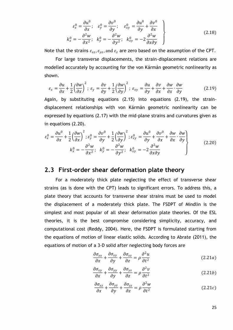
25

휀𝑥0 =

𝜕𝑢0

𝜕𝑥; 휀𝑦

0 =𝜕𝑣0

𝜕𝑦; 휀𝑥𝑦

0 =𝜕𝑢0

𝜕𝑦+𝜕𝑣0

𝜕𝑥

𝑘𝑥0 = −

𝜕2𝑤

𝜕𝑥2; 𝑘𝑦

0 = −𝜕2𝑤

𝜕𝑦2; 𝑘𝑥𝑦

0 = −2𝜕2𝑤

𝜕𝑥𝜕𝑦

(2.18)

Note that the strains 휀𝑥𝑧 , 휀𝑦𝑧 , and 휀𝑧 are zero based on the assumption of the CPT.

For large transverse displacements, the strain-displacement relations are

modelled accurately by accounting for the von Kármán geometric nonlinearity as

shown.

휀𝑥 =𝜕𝑢

𝜕𝑥+

1

2 𝜕𝑤

𝜕𝑥

2

; 휀𝑦 =𝜕𝑣

𝜕𝑦+

1

2 𝜕𝑤

𝜕𝑦

2

; 휀𝑥𝑦 =𝜕𝑢

𝜕𝑦+𝜕𝑣

𝜕𝑥+𝜕𝑤

𝜕𝑥∙𝜕𝑤

𝜕𝑦 (2.19)

Again, by substituting equations (2.15) into equations (2.19), the strain-

displacement relationships with von Kármán geometric nonlinearity can be

expressed by equations (2.17) with the mid-plane strains and curvatures given as

in equations (2.20).

휀𝑥

0 =𝜕𝑢0

𝜕𝑥+

1

2 𝜕𝑤

𝜕𝑥

2

; 휀𝑦0 =

𝜕𝑣0

𝜕𝑦+

1

2 𝜕𝑤

𝜕𝑦

2

; 휀𝑥𝑦0 =

𝜕𝑢0

𝜕𝑦+𝜕𝑣0

𝜕𝑥+𝜕𝑤

𝜕𝑥∙𝜕𝑤

𝜕𝑦

𝑘𝑥0 = −

𝜕2𝑤

𝜕𝑥2; 𝑘𝑦

0 = −𝜕2𝑤

𝜕𝑦2; 𝑘𝑥𝑦

0 = −2𝜕2𝑤

𝜕𝑥𝜕𝑦

2.20

2.3 First-order shear deformation plate theory

For a moderately thick plate neglecting the effect of transverse shear

strains (as is done with the CPT) leads to significant errors. To address this, a

plate theory that accounts for transverse shear strains must be used to model

the displacement of a moderately thick plate. The FSDPT of Mindlin is the

simplest and most popular of all shear deformation plate theories. Of the ESL

theories, it is the best compromise considering simplicity, accuracy, and

computational cost (Reddy, 2004). Here, the FSDPT is formulated starting from

the equations of motion of linear elastic solids. According to Abrate (2011), the

equations of motion of a 3-D solid after neglecting body forces are

𝜕𝜍𝑥𝑥𝜕𝑥

+𝜕𝜍𝑥𝑦

𝜕𝑦+𝜕𝜍𝑥𝑧𝜕𝑧

= 𝜌𝜕2𝑢

𝜕𝑡2 (2.21𝑎)

𝜕𝜍𝑥𝑦

𝜕𝑥+𝜕𝜍𝑦𝑦

𝜕𝑦+𝜕𝜍𝑦𝑧

𝜕𝑧= 𝜌

𝜕2𝑣

𝜕𝑡2 (2.21𝑏)

𝜕𝜍𝑥𝑧𝜕𝑥

+𝜕𝜍𝑦𝑧

𝜕𝑦+𝜕𝜍𝑧𝑧𝜕𝑧

= 𝜌𝜕2𝑤

𝜕𝑡2 (2.21𝑐)

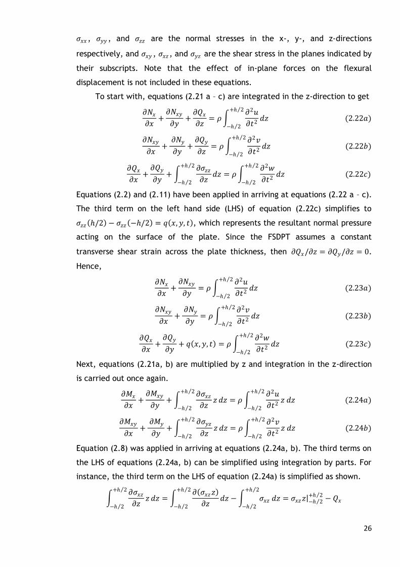
26

𝜍𝑥𝑥 , 𝜍𝑦𝑦 , and 𝜍𝑧𝑧 are the normal stresses in the x-, y-, and z-directions

respectively, and 𝜍𝑥𝑦 , 𝜍𝑥𝑧 , and 𝜍𝑦𝑧 are the shear stress in the planes indicated by

their subscripts. Note that the effect of in-plane forces on the flexural

displacement is not included in these equations.

To start with, equations (2.21 a – c) are integrated in the z-direction to get


+𝜕𝑁𝑥𝑦

𝜕𝑦+𝜕𝑄𝑥𝜕𝑧

= 𝜌 𝜕2𝑢

𝜕𝑡2

+𝑕 2

−𝑕 2 𝑑𝑧 (2.22𝑎)

𝜕𝑁𝑥𝑦

𝜕𝑥+

𝜕𝑁𝑦

𝜕𝑦+𝜕𝑄𝑦

𝜕𝑧= 𝜌

𝜕2𝑣

𝜕𝑡2

+𝑕 2

−𝑕 2 𝑑𝑧 (2.22𝑏)


+𝜕𝑄𝑦

𝜕𝑦+

𝜕𝜍𝑧𝑧𝜕𝑧

+𝑕 2

−𝑕 2 𝑑𝑧 = 𝜌

𝜕2𝑤

𝜕𝑡2

+𝑕 2

−𝑕 2 𝑑𝑧 (2.22𝑐)

Equations (2.2) and (2.11) have been applied in arriving at equations (2.22 a – c).

The third term on the left hand side (LHS) of equation (2.22c) simplifies to

𝜍𝑧𝑧 𝑕/2 − 𝜍𝑧𝑧 −𝑕/2 = 𝑞 𝑥,𝑦, 𝑡 , which represents the resultant normal pressure

acting on the surface of the plate. Since the FSDPT assumes a constant

transverse shear strain across the plate thickness, then 𝜕𝑄𝑥/𝜕𝑧 = 𝜕𝑄𝑦/𝜕𝑧 = 0.

Hence,


+𝜕𝑁𝑥𝑦

𝜕𝑦= 𝜌

𝜕2𝑢

𝜕𝑡2

+𝑕 2

−𝑕 2 𝑑𝑧 (2.23𝑎)

𝜕𝑁𝑥𝑦

𝜕𝑥+

𝜕𝑁𝑦

𝜕𝑦= 𝜌

𝜕2𝑣

𝜕𝑡2

+𝑕 2

−𝑕 2 𝑑𝑧 (2.23𝑏)


+𝜕𝑄𝑦

𝜕𝑦+ 𝑞 𝑥,𝑦, 𝑡 = 𝜌

𝜕2𝑤

𝜕𝑡2

+𝑕 2

−𝑕 2 𝑑𝑧 (2.23𝑐)

Next, equations (2.21a, b) are multiplied by z and integration in the z-direction

is carried out once again.

𝜕𝑀𝑥

𝜕𝑥+𝜕𝑀𝑥𝑦

𝜕𝑦+

𝜕𝜍𝑥𝑧𝜕𝑧

𝑧+𝑕 2

−𝑕 2 𝑑𝑧 = 𝜌

𝜕2𝑢

𝜕𝑡2

+𝑕 2

−𝑕 2 𝑧 𝑑𝑧 (2.24𝑎)

𝜕𝑀𝑥𝑦

𝜕𝑥+

𝜕𝑀𝑦

𝜕𝑦+

𝜕𝜍𝑦𝑧

𝜕𝑧𝑧

+𝑕 2

−𝑕 2 𝑑𝑧 = 𝜌

𝜕2𝑣

𝜕𝑡2

+𝑕 2

−𝑕 2 𝑧 𝑑𝑧 (2.24𝑏)

Equation (2.8) was applied in arriving at equations (2.24a, b). The third terms on

the LHS of equations (2.24a, b) can be simplified using integration by parts. For

instance, the third term on the LHS of equation (2.24a) is simplified as shown.


𝑧+𝑕 2

−𝑕 2 𝑑𝑧 =

𝜕 𝜍𝑥𝑧𝑧

𝜕𝑧

+𝑕 2

−𝑕 2 𝑑𝑧 − 𝜍𝑥𝑧

+𝑕 2

−𝑕 2 𝑑𝑧 = 𝜍𝑥𝑧𝑧 −𝑕 2

+𝑕 2 − 𝑄𝑥

27

𝜍𝑥𝑧𝑧 −𝑕 2 +𝑕 2

is the sum of distributed moments created by the shear stress 𝜍𝑥𝑧

acting on the top and bottom surfaces of the plate. Generally, this sum is zero.

Therefore,


𝑧+𝑕 2

−𝑕 2 𝑑𝑧 = −𝑄𝑥

Similarly, the third term on the LHS of equation (2.24b) simplifies to

𝜕𝜍𝑦𝑧

𝜕𝑧𝑧

+𝑕 2

−𝑕 2 𝑑𝑧 = −𝑄𝑦

Using the above simplifications, equations (2.24a, b) become

𝜕𝑀𝑥


𝜕𝑦− 𝑄𝑥 = 𝜌

𝜕2𝑢

𝜕𝑡2

+𝑕 2

−𝑕 2 𝑧 𝑑𝑧 (2.25𝑎)

𝜕𝑀𝑥𝑦

𝜕𝑥+

𝜕𝑀𝑦

𝜕𝑦− 𝑄𝑦 = 𝜌

𝜕2𝑣

𝜕𝑡2

+𝑕 2

−𝑕 2 𝑧 𝑑𝑧 (2.25𝑏)

The final aspect in the present formulation of vibration model based on the

FSDPT deals with evaluating the RHS of equations (2.23a – c) and (2.25a, b). To

do this, the displacement field of the FSDPT must be known and that is discussed

next.

2.3.1 Strain-displacement relationships for FSDPT

In the FSDPT, the lines perpendicular to the mid-plane before deformation

do not remain so after deformation. The rotations of the mid-plane normal are

accounted for by assuming constant through-thickness transverse shear strains.

Additionally, the transverse normal strain is negligible as in the CPT. The

kinematic assumptions of the FSDPT are expressed mathematically as:

휀𝑧 =𝜕𝑤

𝜕𝑧= 0; 휀𝑥𝑧 =

𝜕𝑢

𝜕𝑧+𝜕𝑤

𝜕𝑥= 𝐶1; 휀𝑦𝑧 =

𝜕𝑣

𝜕𝑧+𝜕𝑤

𝜕𝑦= 𝐶2 (2.26𝑎)

𝐶1 and 𝐶2 are constant through-thickness shear strains in the x-z and y-z plane

respectively. Integrating equations (2.26a) with respect to z gives the

displacement field of the FSDPT as

𝑢 𝑥,𝑦, 𝑧, 𝑡 = 𝑢0 𝑥,𝑦, 𝑡 + 𝑧 𝐶1 −𝜕𝑤

𝜕𝑥

𝑣 𝑥,𝑦, 𝑧, 𝑡 = 𝑣0 𝑥,𝑦, 𝑡 + 𝑧 𝐶2 −𝜕𝑤

𝜕𝑦

𝑤 𝑥, 𝑦, 𝑡 = 𝑤0 𝑥, 𝑦, 𝑡

(2.26𝑏)

Equations (2.26b) can be written in the form

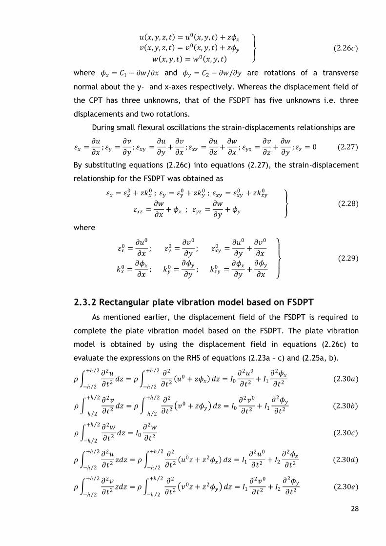
28

𝑢 𝑥,𝑦, 𝑧, 𝑡 = 𝑢0 𝑥,𝑦, 𝑡 + 𝑧𝜙𝑥𝑣 𝑥,𝑦, 𝑧, 𝑡 = 𝑣0 𝑥, 𝑦, 𝑡 + 𝑧𝜙𝑦

𝑤 𝑥,𝑦, 𝑡 = 𝑤0 𝑥, 𝑦, 𝑡

(2.26𝑐)

where 𝜙𝑥 = 𝐶1 − 𝜕𝑤/𝜕𝑥 and 𝜙𝑦 = 𝐶2 − 𝜕𝑤/𝜕𝑦 are rotations of a transverse

normal about the y- and x-axes respectively. Whereas the displacement field of

the CPT has three unknowns, that of the FSDPT has five unknowns i.e. three

displacements and two rotations.

During small flexural oscillations the strain-displacements relationships are

휀𝑥 =𝜕𝑢

𝜕𝑥; 휀𝑦 =

𝜕𝑣

𝜕𝑦; 휀𝑥𝑦 =

𝜕𝑢

𝜕𝑦+𝜕𝑣

𝜕𝑥; 휀𝑥𝑧 =

𝜕𝑢

𝜕𝑧+𝜕𝑤

𝜕𝑥; 휀𝑦𝑧 =

𝜕𝑣

𝜕𝑧+𝜕𝑤

𝜕𝑦; 휀𝑧 = 0 (2.27)

By substituting equations (2.26c) into equations (2.27), the strain-displacement

relationship for the FSDPT was obtained as

휀𝑥 = 휀𝑥

0 + 𝑧𝑘𝑥0 ; 휀𝑦 = 휀𝑦

0 + 𝑧𝑘𝑦0 ; 휀𝑥𝑦 = 휀𝑥𝑦

0 + 𝑧𝑘𝑥𝑦0

휀𝑥𝑧 =𝜕𝑤

𝜕𝑥+ 𝜙𝑥 ; 휀𝑦𝑧 =

𝜕𝑤

𝜕𝑦+ 𝜙𝑦

(2.28)

where

휀𝑥0 =

𝜕𝑢0

𝜕𝑥; 휀𝑦

0 =𝜕𝑣0

𝜕𝑦; 휀𝑥𝑦

0 =𝜕𝑢0

𝜕𝑦+𝜕𝑣0

𝜕𝑥

𝑘𝑥0 =

𝜕𝜙𝑥𝜕𝑥

; 𝑘𝑦0 =

𝜕𝜙𝑦

𝜕𝑦; 𝑘𝑥𝑦

0 =𝜕𝜙𝑥𝜕𝑦

+𝜕𝜙𝑦

𝜕𝑥

(2.29)

2.3.2 Rectangular plate vibration model based on FSDPT

As mentioned earlier, the displacement field of the FSDPT is required to

complete the plate vibration model based on the FSDPT. The plate vibration

model is obtained by using the displacement field in equations (2.26c) to

evaluate the expressions on the RHS of equations (2.23a – c) and (2.25a, b).

𝜌 𝜕2𝑢

𝜕𝑡2

+𝑕 2

−𝑕 2 𝑑𝑧 = 𝜌

𝜕2

𝜕𝑡2 𝑢0 + 𝑧𝜙𝑥

+𝑕 2

−𝑕 2 𝑑𝑧 = 𝐼0

𝜕2𝑢0

𝜕𝑡2+ 𝐼1

𝜕2𝜙𝑥𝜕𝑡2

(2.30𝑎)

𝜌 𝜕2𝑣

𝜕𝑡2

+𝑕 2

−𝑕 2 𝑑𝑧 = 𝜌

𝜕2

𝜕𝑡2 𝑣0 + 𝑧𝜙𝑦

+𝑕 2

−𝑕 2 𝑑𝑧 = 𝐼0

𝜕2𝑣0

𝜕𝑡2+ 𝐼1

𝜕2𝜙𝑦

𝜕𝑡2 (2.30𝑏)

𝜌 𝜕2𝑤

𝜕𝑡2

+𝑕 2

−𝑕 2 𝑑𝑧 = 𝐼0

𝜕2𝑤

𝜕𝑡2 (2.30𝑐)

𝜌 𝜕2𝑢

𝜕𝑡2

+𝑕 2

−𝑕 2 𝑧𝑑𝑧 = 𝜌

𝜕2

𝜕𝑡2 𝑢0𝑧 + 𝑧2𝜙𝑥

+𝑕 2

−𝑕 2 𝑑𝑧 = 𝐼1

𝜕2𝑢0

𝜕𝑡2+ 𝐼2


(2.30𝑑)

𝜌 𝜕2𝑣

𝜕𝑡2

+𝑕 2

−𝑕 2 𝑧𝑑𝑧 = 𝜌

𝜕2

𝜕𝑡2 𝑣0𝑧 + 𝑧2𝜙𝑦

+𝑕 2

−𝑕 2 𝑑𝑧 = 𝐼1

𝜕2𝑣0

𝜕𝑡2+ 𝐼2

𝜕2𝜙𝑦

𝜕𝑡2 (2.30𝑒)

29

where 𝐼0 , 𝐼1, and 𝐼2 are inertia components and they are given by:

𝐼0, 𝐼1, 𝐼2 = 𝜌 1, 𝑧, 𝑧2 +𝑕 2

−𝑕 2 𝑑𝑧 = 𝜌𝑕, 0,

1

12𝜌𝑕3 (2.30𝑓)

𝐼0 is the pure inertia effect, 𝐼1 is the inertia coupling effect between in-plane

and transverse motion, and 𝐼2 is the rotary inertia effect. In general, 𝐼1 = 0.

Substituting equations (2.30a – f) into equations (2.23a – c) and (2.25a, b),

the vibration model of a moderately thick rectangular plate based on the FSDPT

is derived as shown in equations (2.31a – e).


+𝜕𝑁𝑥𝑦

𝜕𝑦= 𝜌𝑕

𝜕2𝑢0

𝜕𝑡2 (2.31𝑎)

𝜕𝑁𝑥𝑦

𝜕𝑥+

𝜕𝑁𝑦

𝜕𝑦= 𝜌𝑕

𝜕2𝑣0

𝜕𝑡2 (2.31𝑏)

𝜕𝑀𝑥


𝜕𝑦− 𝑄𝑥 =

1

12𝜌𝑕3


(2.31𝑐)

𝜕𝑀𝑥𝑦

𝜕𝑥+

𝜕𝑀𝑦

𝜕𝑦− 𝑄𝑦 =

1

12𝜌𝑕3

𝜕2𝜙𝑦

𝜕𝑡2 (2.31𝑑)


+𝜕𝑄𝑦

𝜕𝑦+ 𝑞 𝑥,𝑦, 𝑡 = 𝜌𝑕

𝜕2𝑤

𝜕𝑡2 (2.31𝑒)

2.4 Constitutive equations of laminated rectangular

plates

So far the rectangular plate equations based on the CPT (for thin plates)

and the FSDPT (for moderately thick plates) have been expressed in terms of the

resultant in-plane forces, moments and transverse shear forces. The expressions

for the resultant forces and moments are determined through the constitutive

equations of the plate, which express the behaviour of the plate in terms of

stresses and strains. For a laminated plate, the constitutive equations can be

derived using the ESL approach. This approach represents a laminated plate with

several layers as an equivalent monolithic plate having an aggregate constitutive

behaviour averaged through the thickness. It is a widely used approach and is

capable of giving accurate predictions of the global response of a laminated

plate (Reddy, 2004). Given that the present research is concerned only with the

global vibration response of rectangular plates, the ESL approach has been

applied to develop the constitutive equations for the laminated plate that has

been investigated.

30

Figure 2.6: Sketch illustrating vertical geometry of laminate

} } Layer 1

Layer 2

Layer k

𝑕1

𝑕𝑘

𝑕2

𝑧𝑘−1

−𝑧0

−𝑧1

−𝑧2

𝑧𝑘 } :

:

:

:

:

:

:

:

Mid-plane

−𝑕/2

+𝑕/2

The constitutive equations presented here are for anisotropic plates with

orthotropic layers. By orthotropic, it is meant that a material has properties

differing in three mutually perpendicular directions. Loaded thin and moderately

thick rectangular plates can be said to be in a state of plane stress. The

mechanical stress-strain relationships for a Hookean-orthotropic lamina under

plane stress conditions are (Reddy, 2004)

𝜍𝑥𝜍𝑦𝜍𝑥𝑦𝜍𝑥𝑧𝜍𝑦𝑧

=

𝑄 11 𝑄 12 𝑄 16

𝑄 12 𝑄 22 𝑄 26

𝑄 16 𝑄 26 𝑄 66

0 0 0 0 0 0

0 0 0 0 0 0

𝑄 55 𝑄 45

𝑄 45 𝑄 44

휀𝑥휀𝑦휀𝑥𝑦휀𝑥𝑦휀𝑥𝑦

(2.32)

where

𝑄 11 𝑄 12 𝑄 16

𝑄 12 𝑄 22 𝑄 26

𝑄 16 𝑄 26 𝑄 66

0 0 0 0 0 0

0 0 0 0 0 0

𝑄 55 𝑄 45

𝑄 45 𝑄 44

is the transformed (global) stiffness matrix.

The elements of the transformed stiffness matrix depend on the angle between

the material axes of each lamina and the axes of the laminate. The expressions

for calculating the elements of the transformed stiffness matrix can be found in

numerous texts dealing with composite laminates (e.g. Staab, 1999; Jones, 1999;

Reddy, 2004; Vinson and Sierakowski, 2004).

Figure 2.6: Sketch illustrating vertical geometry of laminate

The stresses on the laminated rectangular plate are discontinuous in the

thickness direction due to change in material properties from one lamina to the

other. To evaluate the force and moment resultants of a laminate the

discontinuous stresses must be integrated. The ESL approach determines the

31

stress integration layerwise (i.e. for each lamina) and sums up the force and

moment resultants for all the layers to get the force and moment resultants for

the laminate. The summation follows a well-defined through-thickness geometry

nomenclature as shown in Figure 2.6. The layers of the laminate are numbered

bottom-up starting from 1 to N and the distances of the layer boundaries are

measured from the mid-plane.

In accordance with the ESL approach, the force and moment resultants of a

rectangular laminate can be evaluated as

𝑁𝑥𝑁𝑦𝑁𝑥𝑦

=

𝜍𝑥𝜍𝑦𝜍𝑥𝑦

𝑧𝑘

𝑧𝑘−1

𝑑𝑧

𝑁

𝑘=1

(2.33𝑎)

𝑀𝑥

𝑀𝑦

𝑀𝑥𝑦

=

𝜍𝑥𝜍𝑦𝜍𝑥𝑦

𝑧𝑘

𝑧𝑘−1

𝑧𝑑𝑧

𝑁

𝑘=1

(2.33𝑏)

𝑄𝑥𝑄𝑦 = 𝒦𝑘

𝜍𝑥𝑧𝜍𝑦𝑧

𝑧𝑘

𝑧𝑘−1

𝑑𝑧

𝑁

𝑘=1

(2.33𝑐)

where 𝑘 is the layer index, and 𝑁 is the total number of layers, and 𝒦 is the

shear correction factor, which is used to account for the fact that the transverse

shear stress has a parabolic distribution across the thickness of the plate instead

of the assumed constant value. The kth layer is bounded by surfaces at 𝑧𝑘 and

𝑧𝑘−1 at the top and bottom respectively.

2.4.1 Constitutive equations for a thin rectangular laminate based

on CPT

The constitutive equations of a thin rectangular laminate can be derived by

using equations (2.32) and (2.17) in equations (2.33a, b) to get


= 𝐴11 𝐴12 𝐴16

𝐴12 𝐴22 𝐴26

𝐴16 𝐴26 𝐴66

휀𝑥0

휀𝑦0

휀𝑥𝑦0

+ 𝐵11 𝐵12 𝐵16

𝐵12 𝐵22 𝐵26

𝐵16 𝐵26 𝐵66

𝑘𝑥0

𝑘𝑦0

𝑘𝑥𝑦0

(2.34𝑎)

𝑀𝑥

𝑀𝑦

𝑀𝑥𝑦

= 𝐵11 𝐵12 𝐵16

𝐵12 𝐵22 𝐵26

𝐵16 𝐵26 𝐵66

휀𝑥0

휀𝑦0

휀𝑥𝑦0

+ 𝐷11 𝐷12 𝐷16

𝐷12 𝐷22 𝐷26

𝐷16 𝐷26 𝐷66

𝑘𝑥0

𝑘𝑦0

𝑘𝑥𝑦0

(2.34𝑏)

𝐴𝑖𝑗 , 𝐵𝑖𝑗 and 𝐷𝑖𝑗 for 𝑖, 𝑗 = 1, 2, 6 are the extensional, bending-extension

coupling, and bending stiffness matrices respectively, and are determined as

32

𝐴𝑖𝑗 = 𝑄 𝑖𝑗𝑘 𝑧𝑘 − 𝑧𝑘−1

𝑁

𝑘=1

𝐵𝑖𝑗 =1

2 𝑄 𝑖𝑗𝑘 𝑧𝑘

2 − 𝑧𝑘−12

𝑁

𝑘=1

𝐷𝑖𝑗 =1

3 𝑄 𝑖𝑗𝑘 𝑧𝑘

3 − 𝑧𝑘−13

𝑁

𝑘=1

(2.35)

𝑄 𝑖𝑗𝑘 is the transformed reduced stiffness of the kth layer of the laminate, and is

related to material properties of the kth layer as shown in equations (2.36),

assuming the material axes of each layer coincides with the laminate axes.

𝑄 11 𝑘 = 𝐸1

1 − 𝜐12𝑣21 𝑘

𝑄 12 𝑘 = 𝜐12𝐸2

1 − 𝜐12𝜐21 𝑘

𝑄 22 𝑘 = 𝐸2

1 − 𝜐12𝜐21 𝑘

𝑄 66 𝑘 = 𝐺12 𝑘 = 𝐸2

2 1 + 𝜐12 𝑘

𝑄 16 𝑘 = 𝑄 26 𝑘 = 0

(2.36)

𝑄 16 𝑘 = 𝑄 26 𝑘 = 0 for orthotropic anisotropy under plane stress, 𝐸 is the

Young’s modulus and 𝜐 is the Poisson’s ratio. The mid-plane strains and

curvatures in equations (2.34a, b) are obtained from equations (2.18) and (2.20)

for small and large flexural displacements respectively.

2.4.2 Constitutive equations for a moderately thick rectangular

laminate based on FSDPT

The constitutive equations of a moderately thick rectangular laminate can

be derived by using equations (2.32) and (2.28) in equations (2.33a – c). For the

in-plane force and moment resultants the constitutive equations are the same as

equations (2.34a, b), but the mid-plane strains and curvatures are obtained from

equation (2.29). For the transverse shear force resultants the constitutive

equations are

𝑄𝑥𝑄𝑦 =

𝐴55 𝐴45

𝐴45 𝐴44 휀𝑥𝑧휀𝑦𝑧

(2.37)

33

where

𝐴𝑖𝑗 = 𝒦𝑘𝑄 𝑖𝑗𝑘 𝑧𝑘 − 𝑧𝑘−1

𝑁

𝑘=1

𝑓𝑜𝑟 𝑖, 𝑗 = 4,5

If the material axes of each layer coincides with the laminate axes then 𝐴45 = 0

and the transverse shear stresses depend on 𝐴44 and 𝐴55 only. In that case,

𝑄 44 𝑘 = 𝐺23 𝑘 and 𝑄 55 𝑘 = 𝐺13 𝑘. 𝒦𝑘 is the shear correction factor for the kth

lamina.

It has been shown that the shear correction factor of a thick isotropic plate

depends on the Poisson’s ratio of the material (Liew et al, 1998). Wittrick (1987)

proposed that the shear correction factor could be determined as 𝒦 = 5/(6 − 𝜐).

Liew et al (1998) suggests that Wittrick’s shear correction formula is preferable

to others incorporating Poisson’s ratio effect because of its simplicity and

accuracy. With thick laminated plates the shear correction factor depends

generally on the laminate properties (Reddy, 2004). Madabhusi-Raman and

Daralos (1996) derived an expression for 𝒦 in algebraic form for a general N-

layer rectangular laminate. Their formula appears to be the most comprehensive

direct expression for calculating 𝒦 that takes into account the laminate

properties. Simpler expressions for orthotropic laminates with rectangular cross-

section have been proposed by Teh and Haung (1979), Dharmarajan and

McCutchen (1973), and Omidvar (1998). Others have used the common value of

𝒦 = 5/6 in studying shear deformable laminated plates (Bert and Chen, 1978; Li

and Mirza, 1995; Reddy, 2004; etc). In the present research, Wittrick’s formula

has been applied to each layer in determining 𝒦 so as to account for the

Poisson’s ratio effect of each lamina of the trimorph plate.

2.5 Determination of the laminate stiffness coefficients

Alternative expressions to equations (2.35) have been presented by Staab

(1999) for the determination of the laminate stiffness coefficients. The stiffness

coefficients were expressed in terms of the distance of each lamina centroid

measured from the mid-plane, and the thickness of the lamina. Big-Alabo and

Cartmell (2011) attempted to simplify algebraically the evaluation of the

stiffness coefficients by expressing them in terms of the lamina thicknesses only.

While this representation is computationally simple, the mid-plane was not

taken into account. Consequently, the bending-extension and bending stiffnesses

34

calculated using this approach are higher than the actual values. Here the mid-

plane has been accounted for and a sign convention has been introduced to

ensure consistency with plate deformation theory and to produce accurate

results. The sign convention requires that lamina boundaries which lie below the

mid-plane are negative while those above the mid-plane are positive (see Figure

2.6). The stiffness coefficients are then expressed in terms of the lamina

thicknesses and the total thickness of the laminate.

From Figure 2.6, the following can be deduced geometrically,

𝑧𝑘 − 𝑧𝑘−1 = 𝑕𝑘

𝑧𝑘 = 𝑕𝑖 − 𝑕/2 ; 𝑘 > 0 𝑜𝑟

𝑘

𝑖=1

𝑧𝑘−1 = 𝑕𝑖 − 𝑕/2 ; 𝑘 > 1

𝑘−1

𝑖=1

(2.38)

where 𝑕𝑘 is the thickness of the kth layer. If the inequalities in equations (2.38b,

c) are not satisfied then 𝑧𝑘 = 0 and 𝑧𝑘−1 = 0.

𝑧𝑘2 − 𝑧𝑘−1

2 = 𝑧𝑘 + 𝑧𝑘−1 𝑧𝑘 − 𝑧𝑘−1 = 𝑧𝑘 − 𝑧𝑘−1 + 2𝑧𝑘−1 𝑧𝑘 − 𝑧𝑘−1

Applying equation (2.38), 𝑧𝑘2 − 𝑧𝑘−1

2 = 𝑕𝑘 + 2𝑧𝑘−1 𝑕𝑘 = 𝑕𝑘 𝑕𝑘 + 2 𝑕𝑖 − 𝑕𝑘−1𝑖=1 .

Also, 𝑧𝑘3 − 𝑧𝑘−1

3 = 𝑧𝑘 − 𝑧𝑘−1 3 + 3 𝑧𝑘 − 𝑧𝑘−1 𝑧𝑘𝑧𝑘−1.

Applying equation (2.38), 𝑧𝑘3 − 𝑧𝑘−1

3 = 𝑕𝑘3 + 3𝑕𝑘 𝑕𝑖

𝑘𝑖=1 − 𝑕/2 𝑕𝑖 − 𝑕/2𝑘−1

𝑖=1 .

Consequently, the extension, bending-extension and bending stiffness

coefficients for i, j = 1, 2, 6 can be determined thus:

𝐴𝑖𝑗 = 𝑄 𝑖𝑗𝑘 𝑕𝑘

𝑁

𝑘=1

𝐵𝑖𝑗 =1

2 𝑄 𝑖𝑗𝑘 𝑕𝑘 𝑕𝑘 + 2 𝑕𝑖 − 𝑕

𝑘−1

𝑖=1

𝑁

𝑘=1

𝐷𝑖𝑗 =1

3 𝑄 𝑖𝑗𝑘 𝑕𝑘

3 + 3𝑕𝑘 𝑕𝑖

𝑘

𝑖=1

− 𝑕/2 𝑕𝑖 − 𝑕/2

𝑘−1

𝑖=1

𝑁

𝑘=1

(2.39𝑎)

Similarly, the shear stiffness coefficients are calculated from

𝐴𝑖𝑗 = 𝒦𝑘𝑄 𝑖𝑗𝑘 𝑕𝑘

𝑁

𝑘=1

𝑓𝑜𝑟 𝑖, 𝑗 = 4,5 2.39𝑏

where 𝒦𝑘 = 5/(6 − 𝜐𝑘). The validity of equations (2.39a) was confirmed by

comparing with results obtained using equations (2.35) and Staab’s expressions

(1999). All three expressions produced exactly the same results for the

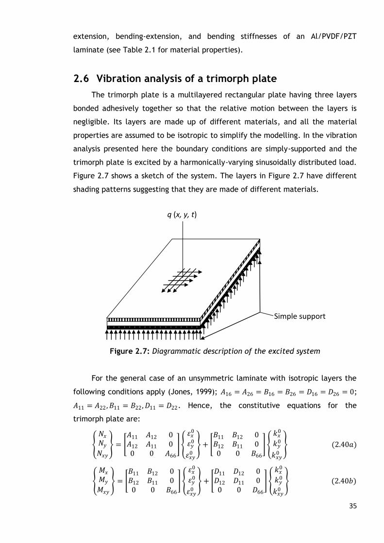
35

q (x, y, t)

Figure 2.7: Diagrammatic description of the system

Simple support

extension, bending-extension, and bending stiffnesses of an Al/PVDF/PZT

laminate (see Table 2.1 for material properties).

2.6 Vibration analysis of a trimorph plate

The trimorph plate is a multilayered rectangular plate having three layers

bonded adhesively together so that the relative motion between the layers is

negligible. Its layers are made up of different materials, and all the material

properties are assumed to be isotropic to simplify the modelling. In the vibration

analysis presented here the boundary conditions are simply-supported and the

trimorph plate is excited by a harmonically-varying sinusoidally distributed load.

Figure 2.7 shows a sketch of the system. The layers in Figure 2.7 have different

shading patterns suggesting that they are made of different materials.

Figure 2.7: Diagrammatic description of the excited system

For the general case of an unsymmetric laminate with isotropic layers the

following conditions apply (Jones, 1999); 𝐴16 = 𝐴26 = 𝐵16 = 𝐵26 = 𝐷16 = 𝐷26 = 0;

𝐴11 = 𝐴22 ,𝐵11 = 𝐵22 ,𝐷11 = 𝐷22. Hence, the constitutive equations for the

trimorph plate are:


= 𝐴11 𝐴12 0𝐴12 𝐴11 0

0 0 𝐴66

휀𝑥0

휀𝑦0

휀𝑥𝑦0

+ 𝐵11 𝐵12 0𝐵12 𝐵11 0

0 0 𝐵66

𝑘𝑥0

𝑘𝑦0

𝑘𝑥𝑦0

(2.40𝑎)

𝑀𝑥

𝑀𝑦

𝑀𝑥𝑦

= 𝐵11 𝐵12 0𝐵12 𝐵11 0

0 0 𝐵66

휀𝑥0

휀𝑦0

휀𝑥𝑦0

+ 𝐷11 𝐷12 0𝐷12 𝐷11 0

0 0 𝐷66

𝑘𝑥0

𝑘𝑦0

𝑘𝑥𝑦0

(2.40𝑏)

36

In this section, the frequency- and time-domain responses of the trimorph

plate are presented for the case of a thin plate and a moderately thick plate.

The in-plane displacements are not considered since the interest is on the

transverse displacement. The aim of the vibration analysis is to demonstrate the

effect of the different possible lamination sequence of a trimorph plate

composed of Al, PVDF, and PZT layers on the dynamic characteristic of the

trimorph plate. Actually, Big-Alabo and Cartmell have carried out such

investigations for small (2011) and large (2012) flexural oscillations of a thin

trimorph plate with the latter being a part of the present research.

Nevertheless, the investigations are repeated here because the expressions used

for calculating the bending-extension and bending stiffnesses in the previous

studies produced values higher than the actual values.

2.6.1 Vibration analysis of a thin trimorph plate

The vibration model for small flexural oscillations of the thin trimorph

plate can be obtained by substituting equations (2.18) and (2.40b) into equation

(2.7), and neglecting in-plane displacements.

𝜌𝑕𝜕2𝑤

𝜕𝑡2+ 𝑐

𝜕𝑤

𝜕𝑡+ 𝐷11

𝜕4𝑤

𝜕𝑥4+𝜕4𝑤

𝜕𝑦4 + 2 𝐷12 + 2𝐷66

𝜕4𝑤

𝜕𝑥2𝜕𝑦2= 𝑞 𝑥,𝑦, 𝑡 (2.41)

For large flexural oscillations of the thin trimorph plate, the vibration model is

obtained by substituting equations (2.20) and (2.40b) into equation (2.13), and

neglecting in-plane displacements.

𝜌𝑕𝜕2𝑤

𝜕𝑡2+ 𝑐

𝜕𝑤

𝜕𝑡+ 𝐷11

𝜕4𝑤

𝜕𝑥4+𝜕4𝑤

𝜕𝑦4 + 2 𝐷12 + 2𝐷66

𝜕4𝑤

𝜕𝑥2𝜕𝑦2

− 𝐵11 𝜕2𝑤

𝜕𝑦2

2

+ 𝜕2𝑤

𝜕𝑥2

2

+ 2𝐵12

𝜕2𝑤

𝜕𝑥2∙𝜕2𝑤

𝜕𝑦2+ 4𝐵66

𝜕2𝑤

𝜕𝑥𝜕𝑦

2

+1

2

𝜕2

𝜕𝑥2 𝐵11

𝜕𝑤

𝜕𝑥

2

+ 𝐵12 𝜕𝑤

𝜕𝑦

2

+1

2

𝜕2

𝜕𝑦2 𝐵12

𝜕𝑤

𝜕𝑥

2

+ 𝐵11 𝜕𝑤

𝜕𝑦

2

+ 2𝐵66

𝜕2

𝜕𝑥𝜕𝑦 𝜕𝑤

𝜕𝑥∙𝜕𝑤

𝜕𝑦 +

1

2 𝐴11

𝜕𝑤

𝜕𝑥

2

+ 𝐴12 𝜕𝑤

𝜕𝑦

2

𝜕2𝑤

𝜕𝑥2

+1

2 𝐴12

𝜕𝑤

𝜕𝑥

2

+ 𝐴11 𝜕𝑤

𝜕𝑦

2

𝜕2𝑤

𝜕𝑦2+ 2𝐴66

𝜕𝑤

𝜕𝑥∙𝜕𝑤

𝜕𝑦∙𝜕2𝑤

𝜕𝑥𝜕𝑦

= 𝑞 𝑥, 𝑦, 𝑡 (2.42)

37

For time-dependent sinusoidally distributed load, the load distribution is given

as 𝑞 𝑥,𝑦, 𝑡 = 𝑞 𝑡 sin(𝜋𝑥/𝑎) sin(𝜋𝑦/𝑏) where 𝑞 𝑡 is considered as a harmonically

varying function for the present investigation. In general, the transverse

displacement and external excitation can be expressed in series form as:

𝑤 𝑥,𝑦, 𝑡 = 𝑊𝑚𝑛 (𝑡)

∞

𝑛=1

∞

𝑚=1

𝑋𝑚𝑌𝑛 (2.43𝑎)

𝑞 𝑥, 𝑦, 𝑡 = 𝑄𝑚𝑛 (𝑡) sin 𝑚𝜋𝑥

𝑎 sin

𝑛𝜋𝑦

𝑏

∞

𝑛=1

∞

𝑚=1

(2.43𝑏)

𝑄𝑚𝑛 (𝑡) =4

𝑎𝑏 𝑞 𝑥,𝑦, 𝑡

𝑏

0

sin 𝑚𝜋𝑥

𝑎 sin

𝑛𝜋𝑦

𝑏 𝑑𝑥𝑑𝑦

𝑎

0

(2.43𝑐)

𝑋𝑚 and 𝑌𝑛 are admissible shape functions that satisfy the boundary conditions

but not necessarily the PDE. For time-dependent sinusoidally distributed load,

the load coefficient simplifies to a closed-form solution that is independent of

the vibration modes i.e. 𝑄𝑚𝑛 𝑡 = 𝑞(𝑡). Equations (2.41) and (2.42) can be

reduced to ODEs using the Galerkin variational approach (Szilard, 2004). The

vibration models have been presented in such a way that the LHS of the

equation is a partial differential expression (PDEx) in terms of the transverse

displacement and the RHS is the external excitation. Thus, the Galerkin

variational formula for derivation of the reduced model can be expressed as

𝑃𝐷𝐸𝑥 − 𝑞 𝑥, 𝑦, 𝑡 𝑎

0

𝑏

0

𝑋𝑚𝑌𝑛𝑑𝑥𝑑𝑦 = 0 (2.44)

For simply-supported boundary condition on all edges of the rectangular plate

(SSSS) 𝑋𝑚 = sin 𝑚𝜋𝑥/𝑎 and 𝑌𝑛 = sin 𝑛𝜋𝑦/𝑏 . Substituting equations (2.41),

(2.42) and (2.43a) in equation (2.44) and evaluating the resulting double integral

for SSSS, the reduced vibration models for the flexural oscillations of the thin

trimorph plate are:

Small oscillations

𝑊 𝑚𝑛 + 𝑐 𝑊 𝑚𝑛 + 𝐷 𝑊𝑚𝑛 = 𝑄 sin𝜔𝑡 (2.45)

Large oscillations

𝑊 𝑚𝑛 + 𝑐 𝑊 𝑚𝑛 + 𝐷 𝑊𝑚𝑛 − 𝐵 𝑊𝑚𝑛2 − 𝐴 𝑊𝑚𝑛

3 = 𝑄 sin𝜔𝑡 (2.46)

where 𝑊𝑚𝑛 is the time-domain flexural displacement of the 𝑚, 𝑛 vibration

mode;

𝑐 =𝑐

𝜌𝑕= 2𝜇 𝐷 ; 𝑄 =

𝑞

𝜌𝑕 are the damping constant per unit mass and excitation

magnitude per unit mass respectively;

38

𝐷 =𝜋4

𝜌𝑕 𝐷11

𝑚4

𝑎4 +𝑛4

𝑏4 +2𝑚2𝑛2 𝐷12 +2𝐷66

𝑎2𝑏2 is the bending stiffness per unit mass;

𝐵 =𝜋2

𝜌𝑕

32

3𝑚𝑛 𝐵11

𝑚4

𝑎4 +𝑛4

𝑏4 +𝑚2𝑛2 𝐵12 +𝐵66

𝑎2𝑏2 is the bending-extension stiffness per

unit mass; and

𝐴 =𝜋4

32𝜌𝑕 3𝐴11

𝑚4

𝑎4 +𝑛4

𝑏4 +𝑚2𝑛2 6𝐴12−4𝐴66

𝑎2𝑏2 is the extensional stiffness per unit

mass.

Equations (2.45) and (2.46) have been solved by means of direct numerical

integration using the NDSolve function in Mathematica™. The plate simulated is

a 1 [m] x 1 [m] square plate with layer thicknesses of 3 [mm], 1 [mm], and 1

[mm] for the Al, PVDF, and PZT layers respectively. The material properties of

the layers are the same as in Big-Alabo and Cartmell (2011) (see Table 2.1) and

the magnitude of the excitation force used for the simulation is 10 [N/m2].

Table 2.1: Material properties of the trimorph plate layers

Material Poisson's ratio, 𝝊 [-] Modulus, E [GPa] Density, ρ [kg/m3]

Al 0.33 70 2700

PVDF 0.44 1.1 1770

PZT 0.3 64 7600

There are six possible lamination sequences of the trimorph plate namely:

Al/PVDF/PZT, Al/PZT/PVDF, PVDF/PZT/Al, PVDF/Al/PZT, PZT/Al/PVDF, and

PZT/PVDF/Al, and the excitation is directly applied on the top layer. Studies

were carried out for the fundamental response mode (𝑚 = 𝑛 = 1) and central

displacement of the trimorph plate (𝑥 = 𝑎/2; 𝑦 = 𝑏/2) using zero initial

conditions (𝑊(0) = 𝑊 (0) = 0). Tables 2.2 and 2.3 show the response

characteristics for the different lamination sequences of the trimorph plate. The

results show that the lamination sequence influences the response

characteristics. This means that the lamination sequence of a multilayer

laminated plate with more than one material composition can be a basis for

selecting the best layer-stacking (Big-Alabo and Cartmell, 2011; 2012). For most

applications, a plate with high bending stiffness or undamped natural frequency

is desirable. This is because a higher bending stiffness results in lower transverse

displacements. According to the results in Tables 2.2 and 2.3 the Al/PVDF/PZT

or PZT/PVDF/Al lamination sequence meets this condition better than the other

lamination sequences.

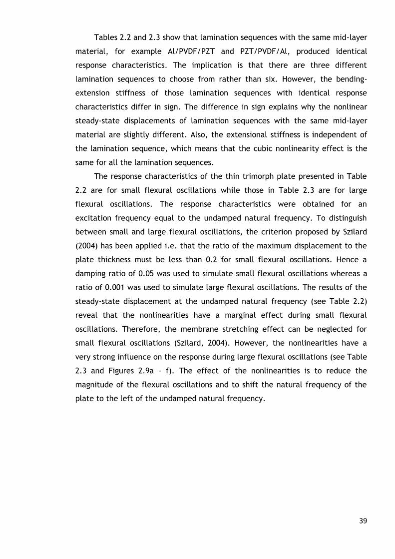
39

Tables 2.2 and 2.3 show that lamination sequences with the same mid-layer

material, for example Al/PVDF/PZT and PZT/PVDF/Al, produced identical

response characteristics. The implication is that there are three different

lamination sequences to choose from rather than six. However, the bending-

extension stiffness of those lamination sequences with identical response

characteristics differ in sign. The difference in sign explains why the nonlinear

steady-state displacements of lamination sequences with the same mid-layer

material are slightly different. Also, the extensional stiffness is independent of

the lamination sequence, which means that the cubic nonlinearity effect is the

same for all the lamination sequences.

The response characteristics of the thin trimorph plate presented in Table

2.2 are for small flexural oscillations while those in Table 2.3 are for large

flexural oscillations. The response characteristics were obtained for an

excitation frequency equal to the undamped natural frequency. To distinguish

between small and large flexural oscillations, the criterion proposed by Szilard

(2004) has been applied i.e. that the ratio of the maximum displacement to the

plate thickness must be less than 0.2 for small flexural oscillations. Hence a

damping ratio of 0.05 was used to simulate small flexural oscillations whereas a

ratio of 0.001 was used to simulate large flexural oscillations. The results of the

steady-state displacement at the undamped natural frequency (see Table 2.2)

reveal that the nonlinearities have a marginal effect during small flexural

oscillations. Therefore, the membrane stretching effect can be neglected for

small flexural oscillations (Szilard, 2004). However, the nonlinearities have a

very strong influence on the response during large flexural oscillations (see Table

2.3 and Figures 2.9a – f). The effect of the nonlinearities is to reduce the

magnitude of the flexural oscillations and to shift the natural frequency of the

plate to the left of the undamped natural frequency.

40

Table 2.2: Response characteristics for small flexural oscillations 𝜇 = 0.05

S/N

Layer Arrangement

1-2-3 respectively

Bending stiffness

𝑫 [N/mkg]

Bending-extensional

stiffness 𝑩 [N/m2kg]

Extensional

stiffness 𝑨 [N/m3kg]

Operating frequency

[rad/s]

Damping constant [Ns/mkg]

Linear steady-state

response (w/h) [ - ]

Nonlinear steady-state


1 Al/PVDF/PZT 15661.2 505768. 3.534×108 125.145 12.515 0.0731 0.0733

2 Al/PZT/PVDF 11039.4 872978. 3.534×108 105.068 10.507 0.104 0.105

3 PVDF/PZT/Al 11039.4 -872978. 3.534×108 105.068 10.507 0.104 0.102

4 PVDF/Al/PZT 10488.1 -734421. 3.534×108 102.412 10.241 0.109 0.106

5 PZT/Al/PVDF 10488.1 734421. 3.534×108 102.412 10.241 0.109 0.109

6 PZT/PVDF/Al 15661.2 -505768. 3.534×108 125.145 12.515 0.0731 0.0727

Table 2.3: Response characteristics for large flexural oscillations 𝜇 = 0.001

S/N

Layer Arrangement

1-2-3 respectively

Bending stiffness

𝑫 [N/mkg]

Bending-extensional

stiffness 𝑩 [N/m2kg]

Extensional

stiffness 𝑨 [N/m3kg]

Operating frequency

[rad/s]

Damping constant [Ns/mkg]

Linear steady-state


Nonlinear steady-state


1 Al/PVDF/PZT 15661.2 505768. 3.534×108 125.145 0.250 3.645 0.257

2 Al/PZT/PVDF 11039.4 872978. 3.534×108 105.068 0.210 5.149 0.250

3 PVDF/PZT/Al 11039.4 -872978. 3.534×108 105.068 0.210 5.149 0.233

4 PVDF/Al/PZT 10488.1 -734421. 3.534×108 102.412 0.205 5.394 0.228

5 PZT/Al/PVDF 10488.1 734421. 3.534×108 102.412 0.205 5.394 0.242

6 PZT/PVDF/Al 15661.2 -505768. 3.534×108 125.145 0.250 3.645 0.249

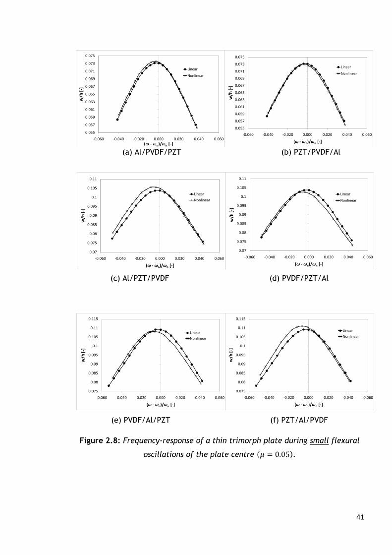
41

0.055

0.057

0.059

0.061

0.063

0.065

0.067

0.069

0.071

0.073

0.075

-0.060 -0.040 -0.020 0.000 0.020 0.040 0.060

w/h

[-]

(ω - ωn)/ωn [-]

Linear

Nonlinear

0.075

0.08

0.085

0.09

0.095

0.1

0.105

0.11

0.115

-0.060 -0.040 -0.020 0.000 0.020 0.040 0.060

w/h

[-]

(ω - ωn)/ωn [-]

Linear

Nonlinear

0.055

0.057

0.059

0.061

0.063

0.065

0.067

0.069

0.071

0.073

0.075

-0.060 -0.040 -0.020 0.000 0.020 0.040 0.060

w/h

[-]

(ω - ωn)/ωn [-]

Linear

Nonlinear

0.07

0.075

0.08

0.085

0.09

0.095

0.1

0.105

0.11

-0.060 -0.040 -0.020 0.000 0.020 0.040 0.060

w/h

[-]

(ω - ωn)/ωn [-]

Linear

Nonlinear

0.07

0.075

0.08

0.085

0.09

0.095

0.1

0.105

0.11

-0.060 -0.040 -0.020 0.000 0.020 0.040 0.060

w/h

[-]

(ω - ωn)/ωn [-]

Linear

Nonlinear

0.075

0.08

0.085

0.09

0.095

0.1

0.105

0.11

0.115

-0.060 -0.040 -0.020 0.000 0.020 0.040 0.060

w/h

[-]

(ω - ωn)/ωn [-]

Linear

Nonlinear

(a) Al/PVDF/PZT (b) PZT/PVDF/Al

(c) Al/PZT/PVDF (d) PVDF/PZT/Al

(e) PVDF/Al/PZT (f) PZT/Al/PVDF

Figure 2.8: Frequency-response of a thin trimorph plate during small flexural

oscillations of the plate centre 𝜇 = 0.05 .

42

0

0.1

0.2

0.3

0.4

0.5

0.6

0.7

0.8

0.9

1

-0.060 -0.040 -0.020 0.000 0.020 0.040 0.060

w/h

[-]

(ω - ωn)/ωn [-]

Linear

Nonlinear

0

0.1

0.2

0.3

0.4

0.5

0.6

0.7

0.8

0.9

1

-0.080 -0.060 -0.040 -0.020 0.000 0.020 0.040 0.060

w/h

[-]

(ω - ωn)/ωn [-]

Linear

Nonlinear

0

0.1

0.2

0.3

0.4

0.5

0.6

0.7

0.8

0.9

1

-0.080 -0.060 -0.040 -0.020 0.000 0.020 0.040 0.060

w/h

[-]

(ω - ωn)/ωn [-]

Linear

Nonlinear

0

0.1

0.2

0.3

0.4

0.5

0.6

0.7

0.8

0.9

1

-0.060 -0.040 -0.020 0.000 0.020 0.040 0.060

w/h

[-]

(ω - ωn)/ωn [-]

Linear

Nonlinear

0

0.1

0.2

0.3

0.4

0.5

0.6

0.7

0.8

0.9

1

-0.080 -0.060 -0.040 -0.020 0.000 0.020 0.040 0.060

w/h

[-]

(ω - ωn)/ωn [-]

Linear

Nonlinear

0

0.1

0.2

0.3

0.4

0.5

0.6

0.7

0.8

0.9

1

-0.080 -0.060 -0.040 -0.020 0.000 0.020 0.040 0.060

w/h

[-]

(ω - ωn)/ωn [-]

Linear

Nonlinear

(a) Al/PVDF/PZT (b) PZT/PVDF/Al

(c) Al/PZT/PVDF (d) PVDF/PZT/Al

(e) PVDF/Al/PZT (f) PZT/Al/PVDF

Figure 2.9: Frequency-response of a thin trimorph plate during large flexural

oscillations of the plate centre 𝜇 = 0.001 .

Figures 2.8a – f show the frequency-response for small flexural oscillations

while Figures 2.9a – f show the frequency-response for large flexural oscillations.

These figures reveal that the nonlinear effects due to membrane stretching are

negligible for small flexural oscillations, whereas they are significant for large

flexural oscillations. Since the frequency-response plots were generated by

43

solving the reduced models using numerical integration, only one response value

was obtained for each excitation frequency. Consequently, both the peak

displacement and the corresponding natural frequency of the nonlinear case are

not shown in Figures 2.9a – f. In principle there could be more than one

nonlinear steady-state response at some excitation frequencies. The complete

frequency-response plot for the nonlinear case can be obtained from

approximate analytical solutions derived using perturbation analysis, but this is

not considered here as the present study is intended to show that membrane

stretching effect cannot be neglected during large flexural oscillations.

The reduced nonlinear model (equation 2.46) contains quadratic and cubic

nonlinearities. To examine the effect of these nonlinearities on the response of

the trimorph plate, frequency-response plots were generated in which either of

these nonlinearities could be neglected. Figure 2.10 shows a comparison of the

frequency-response for the three possible cases: (a) only the quadratic

nonlinearity is considered; (b) only the cubic nonlinearity is considered, and (c)

both the quadratic and cubic nonlinearities are considered. The figure reveals

that the cubic nonlinearity (case b) produces a much stronger effect than the

quadratic nonlinearity (case a). The effect of the quadratic nonlinearity is

apparently negligible when both nonlinearities are considered (see cases b and

c). Hence, it can be concluded that the nonlinear response of the trimorph plate

during large flexural oscillations as modelled here is largely determined by the

cubic nonlinearity. This information can be useful for ordering the terms during

perturbation analysis. Such analyses are not covered here as they are beyond the

scope of the present research.

Time-domain response plots were obtained for the Al/PVDF/PZT lamination

sequence. Figures 2.11a, b show the transient and steady-state responses during

small flexural oscillation, and the plots confirm that the nonlinearities due to

membrane stretching do not affect the time-domain response during small

flexural oscillation. In the case of large flexural oscillations, Figures 2.12a, b

show that the steady-state flexural oscillations predicted by the reduced linear

model are much higher than that predicted by the reduced nonlinear model. The

nonlinear response settles more quickly to a steady-state response compared to

the linear response. In conclusion, the linear model over-predicts the magnitude

of flexural oscillations of the trimorph plate during large flexural oscillations.

44

0.055

0.255

0.455

0.655

0.855

1.055

1.255

-0.05 -0.04 -0.03 -0.02 -0.01 0 0.01 0.02 0.03 0.04 0.05

w/h

[-]

(ω - ωn)/ωn [-]

Quad nonlinearity

Cubic nonlinearity

Quad and Cubic nonlinearity

99.80 99.85 99.90 99.95 100.00

0.06

0.04

0.02

0.00

0.02

0.04

0.06

t s

W

h

Linear

Nonlinear

0.0 0.1 0.2 0.3 0.4 0.5

0.06

0.04

0.02

0.00

0.02

0.04

0.06

t s

W

h

Linear

Nonlinear

Figure 2.10: Effect of nonlinear terms on the frequency-response of a thin

trimorph plate undergoing large flexural oscillations μ = 0.001 .

Figure 2.11a: Transient response of a thin Al/PVDF/PZT plate during small

flexural oscillations when excited at the undamped natural frequency.

Figure 2.11b: Steady-state response of a thin Al/PVDF/PZT plate during small


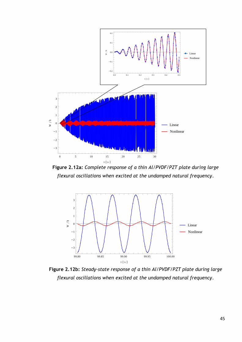
45

99.80 99.85 99.90 99.95 100.00

3

2

1

0

1

2

3

t s

W

h

Linear

Nonlinear

0 5 10 15 20 25 30

3

2

1

0

1

2

3

t s

W

h

Linear

Nonlinear

0.0 0.1 0.2 0.3 0.4 0.5

0.2

0.1

0.0

0.1

0.2

t s

W

h

Linear

Nonlinear

Figure 2.12a: Complete response of a thin Al/PVDF/PZT plate during large


Figure 2.12b: Steady-state response of a thin Al/PVDF/PZT plate during large


46

2.6.2 Vibration analysis of a moderately thick trimorph plate

Large flexural oscillations are uncommon, and in some cases impractical,

during the excitation of moderately thick to thick plates. As a result, the present

analysis of a moderately thick trimorph plate is restricted to small flexural

oscillations. The vibration model for small flexural oscillations of a moderately

thick trimorph plate can be derived by substituting equations (2.28), (2.40b) and

(2.37) into equations (2.31 c – e). After neglecting the in-plane displacements,

the following equations are derived.

𝐷11

𝜕2𝜙𝑥𝜕𝑥2

+ 𝐷12 + 𝐷66 𝜕2𝜙𝑦

𝜕𝑥𝜕𝑦+ 𝐷66

𝜕2𝜙𝑥𝜕𝑦2

− 𝐴55 𝜕𝑤

𝜕𝑥+ 𝜙𝑥 =

𝜌𝑕3

12


(2.47𝑎)

𝐷11

𝜕2𝜙𝑦

𝜕𝑦2+ 𝐷12 + 𝐷66

𝜕2𝜙𝑥𝜕𝑥𝜕𝑦

+ 𝐷66

𝜕2𝜙𝑦

𝜕𝑥2− 𝐴44

𝜕𝑤

𝜕𝑦+ 𝜙𝑦 =

𝜌𝑕3

12

𝜕2𝜙𝑦

𝜕𝑡2 (2.47𝑏)

𝐴55 𝜕2𝑤

𝜕𝑥2+𝜕𝜙𝑥𝜕𝑥

+ 𝐴44 𝜕2𝑤

𝜕𝑦2+𝜕𝜙𝑦

𝜕𝑦 + 𝑞 𝑥,𝑦, 𝑡 = 𝜌𝑕

𝜕2𝑤

𝜕𝑡2 (2.47𝑐)

The solution to equations (2.47a – c) can be expressed in series form as

𝜙𝑥 𝑥,𝑦, 𝑡 = 𝐴𝑚𝑛 (𝑡)

∞

𝑛=1

∞

𝑚=1

𝑋1𝑚𝑌𝑛 (2.48𝑎)

𝜙𝑦 𝑥,𝑦, 𝑡 = 𝐵𝑚𝑛 (𝑡)

∞

𝑛=1

∞

𝑚=1

𝑋𝑚𝑌1𝑛 (2.48𝑏)

𝑤 𝑥, 𝑦, 𝑡 = 𝑊𝑚𝑛 (𝑡)

∞

𝑛=1

∞

𝑚=1

𝑋𝑚𝑌𝑛 (2.48𝑐)

𝐴𝑚𝑛 (𝑡), 𝐵𝑚𝑛 (𝑡), and 𝑊𝑚𝑛 (𝑡) are time-dependent coefficients to be determined.

The shape functions for SSSS are defined as 𝑋1𝑚 = cos 𝑚𝜋𝑥/𝑎 , 𝑌1𝑛 =

cos 𝑛𝜋𝑦/𝑏 , with 𝑋𝑚 and 𝑌𝑛 expressed as defined above. If equations (2.47a – c)

are rearranged such that the RHS is equal to zero, the Galerkin approach can

expressed as

𝐿𝐻𝑆 𝑎

0

𝑏

0

𝜑 𝑥, 𝑦 𝑑𝑥𝑑𝑦 = 0 (2.49)

𝜑 𝑥,𝑦 represents the product of the shape functions in the x- and y-directions.

𝜑 𝑥,𝑦 = 𝑋1𝑚𝑌𝑛 , 𝑋𝑚𝑌1𝑛 , and 𝑋𝑚𝑌𝑛 for equations (2.47a, b, and c) respectively.

Substituting equations (2.47a – c), (2.48a – c) and (2.43a) in equation (2.49) and

evaluating the resulting double integrals, the reduced ODE models are derived

after some algebraic simplification as

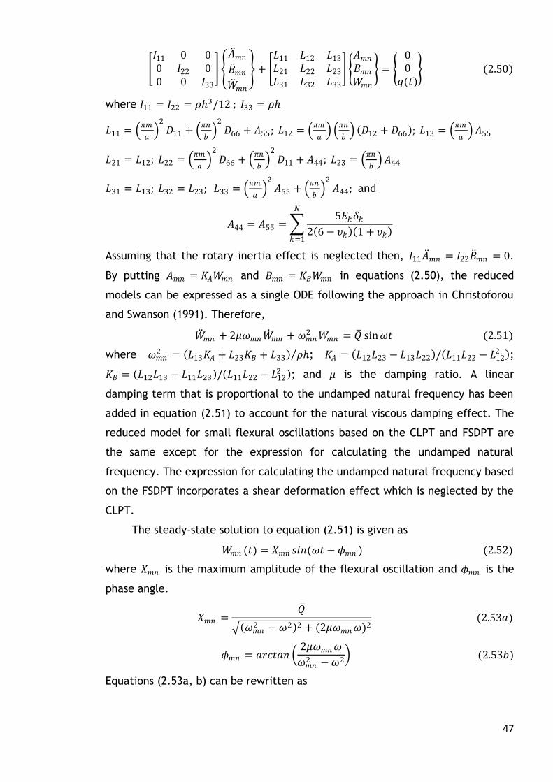
47

𝐼11 0 00 𝐼22 00 0 𝐼33

𝐴 𝑚𝑛𝐵 𝑚𝑛𝑊 𝑚𝑛

+ 𝐿11 𝐿12 𝐿13

𝐿21 𝐿22 𝐿23

𝐿31 𝐿32 𝐿33

𝐴𝑚𝑛𝐵𝑚𝑛𝑊𝑚𝑛

= 00

𝑞(𝑡) (2.50)

where 𝐼11 = 𝐼22 = 𝜌𝑕3/12 ; 𝐼33 = 𝜌𝑕

𝐿11 = 𝜋𝑚

𝑎

2

𝐷11 + 𝜋𝑛

𝑏

2

𝐷66 + 𝐴55; 𝐿12 = 𝜋𝑚

𝑎

𝜋𝑛

𝑏 𝐷12 + 𝐷66 ; 𝐿13 =

𝜋𝑚

𝑎 𝐴55

𝐿21 = 𝐿12; 𝐿22 = 𝜋𝑚

𝑎

2

𝐷66 + 𝜋𝑛

𝑏

2

𝐷11 + 𝐴44; 𝐿23 = 𝜋𝑛

𝑏 𝐴44

𝐿31 = 𝐿13; 𝐿32 = 𝐿23; 𝐿33 = 𝜋𝑚

𝑎

2

𝐴55 + 𝜋𝑛

𝑏

2

𝐴44; and

𝐴44 = 𝐴55 = 5𝐸𝑘𝛿𝑘

2 6 − 𝜐𝑘 1 + 𝜐𝑘

𝑁

𝑘=1

Assuming that the rotary inertia effect is neglected then, 𝐼11𝐴 𝑚𝑛 = 𝐼22𝐵 𝑚𝑛 = 0.

By putting 𝐴𝑚𝑛 = 𝐾𝐴𝑊𝑚𝑛 and 𝐵𝑚𝑛 = 𝐾𝐵𝑊𝑚𝑛 in equations (2.50), the reduced

models can be expressed as a single ODE following the approach in Christoforou

and Swanson (1991). Therefore,

𝑊 𝑚𝑛 + 2𝜇𝜔𝑚𝑛𝑊 𝑚𝑛 + 𝜔𝑚𝑛2 𝑊𝑚𝑛 = 𝑄 sin𝜔𝑡 (2.51)

where 𝜔𝑚𝑛2 = 𝐿13𝐾𝐴 + 𝐿23𝐾𝐵 + 𝐿33 𝜌𝑕 ; 𝐾𝐴 = 𝐿12𝐿23 − 𝐿13𝐿22 / 𝐿11𝐿22 − 𝐿12

2 ;

𝐾𝐵 = 𝐿12𝐿13 − 𝐿11𝐿23 / 𝐿11𝐿22 − 𝐿122 ; and 𝜇 is the damping ratio. A linear

damping term that is proportional to the undamped natural frequency has been

added in equation (2.51) to account for the natural viscous damping effect. The

reduced model for small flexural oscillations based on the CLPT and FSDPT are

the same except for the expression for calculating the undamped natural

frequency. The expression for calculating the undamped natural frequency based

on the FSDPT incorporates a shear deformation effect which is neglected by the

CLPT.

The steady-state solution to equation (2.51) is given as

𝑊𝑚𝑛 (𝑡) = 𝑋𝑚𝑛 𝑠𝑖𝑛(𝜔𝑡 − 𝜙𝑚𝑛 ) (2.52)

where 𝑋𝑚𝑛 is the maximum amplitude of the flexural oscillation and 𝜙𝑚𝑛 is the

phase angle.

𝑋𝑚𝑛 =𝑄

𝜔𝑚𝑛2 −𝜔2 2 + (2𝜇𝜔𝑚𝑛𝜔)2

(2.53𝑎)

𝜙𝑚𝑛 = 𝑎𝑟𝑐𝑡𝑎𝑛 2𝜇𝜔𝑚𝑛𝜔

𝜔𝑚𝑛2 −𝜔2

(2.53𝑏)

Equations (2.53a, b) can be rewritten as

48

𝑋𝑚𝑛 =𝛿𝑠𝑡

1 − 𝛽𝑚𝑛2 2 + (2𝜇𝛽𝑚𝑛 )2 (2.54𝑎)

𝜙𝑚𝑛 = 𝑎𝑟𝑐𝑡𝑎𝑛 2𝜇𝛽𝑚𝑛

1 − 𝛽𝑚𝑛2 (2.54𝑏)

where 𝛿𝑠𝑡 = 𝑄 /𝜔𝑚𝑛2 is the static deflection of the plate and 𝛽𝑚𝑛 = 𝜔/𝜔𝑚𝑛 is the

frequency ratio. At resonance 𝛽𝑚𝑛 = 1, 𝑋𝑚𝑛 = 𝛿𝑠𝑡/2𝜇 and 𝜙𝑚𝑛 = 𝜋/2.

To simulate the dynamic response of the moderately thick trimorph plate,

a 100 [mm] x 100 [mm] square plate with layer thicknesses of 8 [mm], 1 [mm],

and 1 [mm] for the Al, PVDF, and PZT layers was investigated. The plate

thickness to length ratio is 1/10, which is within the limits for moderately thick

plates. The material properties of the layers are the same as in Table 2.1 and a

damping ratio of 10−5 was used in the simulation. The results for the modal

frequencies and steady-state displacements are shown in Table 2.4. A

comparison is made between the results obtained from the CLPT model

(equation 2.45) and those obtained from the FSDPT model (equation 2.51), and

it is observed that the effect of shear deformation as modelled by the present

FSDPT is more pronounced at higher vibration modes. Since the actual transverse

displacement can be approximated by the sum of the contributions of a finite

number of participating modes, then the CLPT model would produce significant

errors when it used to model the vibration response of a moderately thick plate.

Table 2.4: Modal frequencies and responses of a moderately thick Al/PVDF/PZT

plate during small flexural oscillations

Mode Natural frequency [rad/s] Modal displacement [w/h x 10-3]

CLPT FSDPT CLPT FSDPT

1 1 26129.9 25480.7 2.36458 2.4866

1 3 130649 116483 0.0945832 0.118988

1 5 339688 262791 0.0139916 0.023378

3 1 130649 116483 0.0945832 0.118988

3 3 235169 194332 0.0291923 0.0427505

3 5 444208 324206 0.00818194 0.0153598

5 1 339688 262791 0.0139916 0.023378

5 3 444208 324206 0.00818194 0.0153598

5 5 653247 431667 0.00378333 0.00866427

Time-domain responses for the fundamental mode of vibration are shown in

Figures 2.13a, b. Again a comparison is made between the CLPT model and the

49

FSDPT model during the initial phase of the transient response and during the

steady-state response. For both the transient and steady-state responses a phase

difference occurs and the magnitudes of the oscillations differ. As expected, the

phase difference and the difference in the displacements evolve during the

transient response and become constant in the steady-state response.

Figure 2.13a: Transient response of a moderately thick Al/PVDF/PZT plate


frequency.

Figure 2.13b: Steady-state response of a moderately thick Al/PVDF/PZT plate


frequency.

2.7 Chapter conclusions

This chapter presents a detailed formulation of vibration models for thin

and thick rectangular laminated plates, and investigations on the vibration

response of a three-layer rectangular laminate called trimorph plate. For the

50

thin trimorph plate, small and large displacements were investigated and the

results reveal that membrane stretching effect could be neglected in the former

but not in the later. The membrane stretching effect was modelled by

incorporating the von Kármán geometric nonlinearity in the strain-displacement

relationship and accounting for the effect of the induced in-plane forces on the

flexural oscillations. The final reduced model for large displacements was a

forced oscillator with quadratic and cubic nonlinearities, of which the cubic

nonlinearity was found to be more influential than the quadratic nonlinearity.

Simulations run for a moderately thick trimorph plate using the CLPT and

FSDPT models showed that shear deformation effects are more pronounced at

higher modes. The comparison also revealed that significant errors could be

introduced in the determination of the natural frequency and the magnitude of

the flexural oscillations when the CLPT model is used to analyse the vibration

response of a moderately thick trimorph plate because the CLPT model neglects

the shear deformation effect.

Investigations into the response characteristics revealed that the

lamination sequence of the trimorph plate influenced the response of the plate.

Those lamination sequences with the same mid-layer material produced

matching response characteristics except for the bending-extension stiffnesses

that were found to be equal in magnitude but opposite in sign. The implication is

that the best lamination sequence for a given application could be determined

from three lamination sequences instead of six possible lamination sequences.

The extensional stiffness was found to be the same for all possible lamination

sequences, and this means that the effect of the cubic nonlinearity is

independent of the lamination sequence.

The relevance of the vibration analysis presented in this chapter is two-

fold. First, the vibration models developed here could be used for modelling the

impact response of thin and moderately thick laminated plates. An application

of the vibration models in modelling the impact response of the trimorph plate is

discussed in chapter four. Second, the investigations on the response

characteristics of the trimorph plate provide insight into its dynamic behaviour

and form a basis for informative determination of the lamination sequence that

could be used for further studies, e.g. impact analysis, considering the intended

application.

51

CHAPTER THREE

CONTACT MODEL FOR ELASTOPLASTIC INDENTATION

Chapter summary

Accidental load in the form of impact between a rigid object and a

compliant target is a common engineering problem. During such impact there is

a surface interaction between the rigid object and the target known as contact.

Contact models account for the local response (displacement, force, stress, etc)

of the rigid object and the target, and they are necessary for more rigorous

analysis of the dynamics of the impact system. This chapter presents a new

analytical contact model for quasi-static elastoplastic indentation of a half-

space by a rigid spherical mass. First, other published contact models for

elastoplastic indentation of isotropic and transversely isotropic materials are

reviewed. The review is followed by formulation of the new contact model and

then, validation of the proposed model using published experimental data. The

results of the present contact model are found to be in agreement with the

static and dynamic indentation measurements to which they were compared.

3.1 Review of contact models for spherical indentation of

elastoplastic half-space

Contact phenomena finds application in many impact processes such as

forging, stamping, shot-peening, granular flow in industrial processes and solid

object impact on structures. Contact models are normally formulated based on

half-space conditions i.e. the local indentation is much smaller than the size of

the indented surface. For instance, the Hertz contact model gives the force-

indentation relationship for quasi-static loading of a spherical indenter on an

elastic half-space. A detailed treatment of the Hertz contact model for different

contacting surfaces can be found in Johnson (1985) and Goldsmith (2001). The

Hertz contact model is only applicable to small indentations that are elastic, for

which the stress in the contact zone is less than the yield stress of the material

of the indented surface. When the stress in the contact zone is higher than the

yield stress of the material of the indented surface, post-yield effects such as

52

R

𝑉0 R

δ

a

R

𝑉𝑓

𝛿 𝑓

a

(a) (b) (c)

plastic deformation and/or damage occur and significant deviations from the

Hertz contact model are observed (Abrate, 1998).

It has been shown that during impact of a rigid steel ball on a medium hard

steel slab yielding occurs at an impact velocity as low as 0.14 [m/s] (Johnson,

1985). Moreover, most practical impact events are characterised by post-yield

deformation (Johnson, 1985; Goldsmith, 2001), and therefore it is necessary to

account for post-yield deformation effects in the contact model. The effect of

the post-yield deformation is to reduce the contact force from that predicted by

purely elastic deformations and to produce a permanent indentation at the end

of the contact, thereby, making the unloading path different from that of

loading. Figure 3.1 shows a sketch of the impact of a spherical mass on an

elastoplastic half-space.

Figure 3.1: Elastoplastic half-space impact of a rigid spherical indenter on a

compliant flat target (a) before impact (b) during impact (c) after impact.

Contact models that account for post-yield deformation have been

developed for metallic targets (Johnson, 1985; Goldsmith, 2001; Stronge, 2000a;

Li et al, 2002; Brake, 2012) and for composite laminate targets (Cairns, 1991;

Yigit and Christoforou, 1994; Majeed et al, 2012). These models can be divided

into two general groups, namely: those that are developed based on two distinct

loading regimes (Goldsmith 2001; Cairns, 1991; Yigit and Christoforou, 1994;

Majeed et al, 2012) and those that are developed based on three distinct loading

regimes (Johnson, 1985; Stronge 2000a; Li et al, 2002; Brake, 2012). With

metallic targets, three loading regimes (elastic, elastoplastic and fully plastic)

and an unloading regime are required for complete description of the contact

mechanics (Tabor, 1951; Johnson, 1985; Stronge, 2000a). For a contact model

that is based on elastic-elastoplastic-fully plastic loading regimes, the loading

53

features and force-indentation relationships for the elastic and fully (perfectly)

plastic loading regimes are well established. In general, the elastic loading

regime starts from the beginning of the loading and ends at the yield point

where the mean contact pressure is given as 𝑃𝑜𝑦 = 1.1𝑆𝑦 (𝑆𝑦 is the yield stress of

the target). The elastic loading regime can be modelled accurately using the

well-known Hertz contact model. The fully plastic loading regime is

characterised by a linear force-indentation relationship and a constant mean

pressure of 𝑃𝑜𝑝 = 2.8𝑆𝑦, which is equal to the Brinell hardness of the target

(Brake, 2012). The onset of the fully plastic regime occurs at the point where

the mean pressure is 2.8𝑆𝑦 . The main difficulty lies in formulating an analytical

model for the elastoplastic loading regime which starts at the yield point and

ends at the onset of fully plastic conditions. Selected published models for post-

yield indentation of metallic and composite laminate targets are discussed next.

3.1.1 Contact models for post-yield indentation of a metallic half-

space

Figure 3.2: Elastoplastic deformation at (a) yield (b) the onset of fully plastic

loading regime. The cross-hatched area is the surrounding elastically-deformed

material while the unshaded area is the plastically-deformed material.

During post-yield contact loading of a metallic half-space by a rigid

spherical indenter, the elastoplastic loading regime is initiated immediately

after the metal yields. As a result of yielding, a plastically-deformed material

appears below the contact surface at a depth of about half the contact radius

(Figure 3.2a). This plastically-deformed material is completely enclosed within a

surrounding elastically-deformed material (Johnson, 1985). As the elastoplastic

(a) (b)

δ

a

0.4

5a

R

δ

a

0.4

5a

R

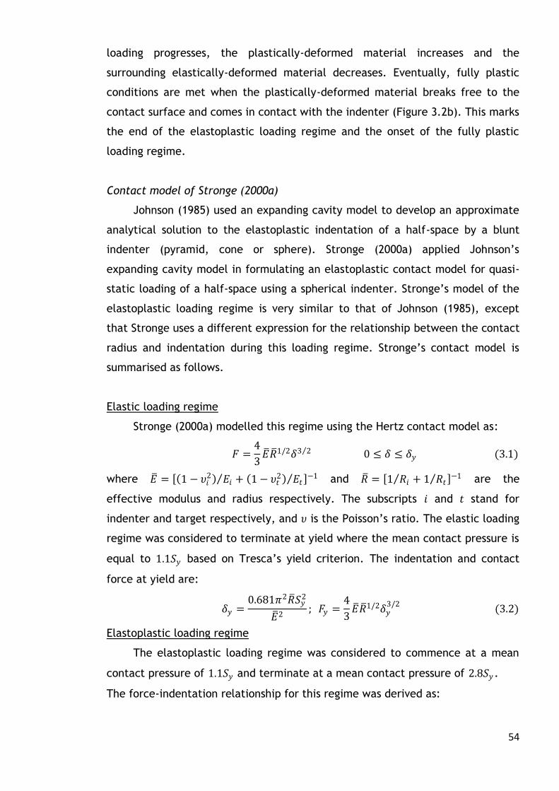
54

loading progresses, the plastically-deformed material increases and the

surrounding elastically-deformed material decreases. Eventually, fully plastic

conditions are met when the plastically-deformed material breaks free to the

contact surface and comes in contact with the indenter (Figure 3.2b). This marks

the end of the elastoplastic loading regime and the onset of the fully plastic

loading regime.

Contact model of Stronge (2000a)

Johnson (1985) used an expanding cavity model to develop an approximate

analytical solution to the elastoplastic indentation of a half-space by a blunt

indenter (pyramid, cone or sphere). Stronge (2000a) applied Johnson’s

expanding cavity model in formulating an elastoplastic contact model for quasi-

static loading of a half-space using a spherical indenter. Stronge’s model of the

elastoplastic loading regime is very similar to that of Johnson (1985), except

that Stronge uses a different expression for the relationship between the contact

radius and indentation during this loading regime. Stronge’s contact model is

summarised as follows.

Elastic loading regime

Stronge (2000a) modelled this regime using the Hertz contact model as:

𝐹 =4

3𝐸 𝑅 1/2𝛿3 2 0 ≤ 𝛿 ≤ 𝛿𝑦 (3.1)

where 𝐸 = 1 − 𝜐𝑖2 𝐸𝑖 + 1 − 𝜐𝑡

2 𝐸𝑡 −1 and 𝑅 = 1 𝑅𝑖 + 1 𝑅𝑡 −1 are the

effective modulus and radius respectively. The subscripts 𝑖 and 𝑡 stand for

indenter and target respectively, and 𝜐 is the Poisson’s ratio. The elastic loading

regime was considered to terminate at yield where the mean contact pressure is

equal to 1.1𝑆𝑦 based on Tresca’s yield criterion. The indentation and contact

force at yield are:

𝛿𝑦 =0.681𝜋2𝑅 𝑆𝑦

2

𝐸 2; 𝐹𝑦 =

4

3𝐸 𝑅 1/2𝛿𝑦

3/2 (3.2)

Elastoplastic loading regime

The elastoplastic loading regime was considered to commence at a mean

contact pressure of 1.1𝑆𝑦 and terminate at a mean contact pressure of 2.8𝑆𝑦 .

The force-indentation relationship for this regime was derived as:

55

𝐹 = 𝐹𝑦 2𝛿

𝛿𝑦− 1 1 +

1

3.3𝑙𝑛

2𝛿

𝛿𝑦− 1 𝛿𝑦 ≤ 𝛿 ≤ 𝛿𝑝 (3.3)

Stronge (2000a) used 𝑎/𝑎𝑦 = 2𝛿/𝛿𝑦 − 1 1/2

to approximate the relationship

between the contact radius and indentation in arriving at equation (3.3).

Johnson (1985) used 𝑎/𝑎𝑦 = 2𝛿/𝛿𝑦 1/2

based on the generally accepted

approximation that 𝑎2 = 2𝑅 𝛿 for indentation beyond the yield point. This

distinction forms the main difference in the models for elastoplastic loading as

presented by Stronge (2000a) and Johnson (1985). Also, Stronge’s model

estimates the end of the elastoplastic loading as 𝛿𝑝 ≅ 82.5𝛿𝑦 whereas Johnson’s

model gives an estimate of 𝛿𝑝 ≅ 73𝛿𝑦 .

Fully plastic loading regime

This loading regime was modelled using a linear force-indentation

relationship based on a constant mean pressure of 𝑃0𝑝 = 2.8𝑆𝑦 , and the contact

radius–indentation relationship used was the same as in the elastoplastic loading

regime.

𝐹 = 2.545𝐹𝑦 2𝛿

𝛿𝑦− 1 𝛿𝑝 ≤ 𝛿 ≤ 𝛿𝑚 (3.4)

Restitution

The restitution was modelled as an elastic unloading with a plastic

deformation effect for post-yield indentation. As a result of plastic deformation,

the model accounts for a permanent indentation 𝛿𝑓 at the end of the unloading

and the effective radius is replaced by a deformed effective radius, 𝑅 𝑑.

𝐹 =4

3𝐸 𝑅 𝑑

1/2 𝛿 − 𝛿𝑓 3 2

𝛿𝑓 ≤ 𝛿 ≤ 𝛿𝑚 (3.5𝑎)

where

𝛿𝑓 = 𝛿𝑚 − 3𝐹𝑚

4𝐸 𝑅 𝑑1/2

2 3

; 𝑅 𝑑 = 𝑅 2𝛿/𝛿𝑦 − 1 𝛿 > 𝛿𝑦

𝑅 𝛿 ≤ 𝛿𝑦 (3.5𝑏, 𝑐)

𝐹𝑚 and 𝛿𝑚 are the maximum contact force and indentation respectively, and

they could be located in any of the loading regimes. When they are located in

the elastic loading regime, there is no post-yield effect and 𝛿𝑓 = 0.

The model for the elastoplastic loading regime is a logarithmic function of

indentation and cannot be expressed in the form of Meyer’s law i.e. 𝐹 = 𝐾𝑐𝛿𝑞

where 𝐾𝑐 is the contact stiffness and 𝑞 ≥ 1 is an exponent defining the

compliance relationship (Goldsmith, 2001). When this model is used for dynamic

56

impact analysis, it has the potential to introduce computational difficulties due

to the more complex nonlinear form in which it is expressed. This may explain

why analytical studies on the impact response of metallic targets using this

elastoplastic contact model are scarce despite the success of the model in

predicting the elastoplastic loading response of metals under static conditions.

Contact model of Li et al (2002)

Li et al (2002) developed a theoretical contact model for the elastoplastic

loading of a half-space using a spherical indenter by assuming a truncated

Hertzian pressure distribution for post-yield indentation. According to this

model, the elastoplastic loading regime is assumed to commence at a mean

contact pressure of 1. 6𝑆𝑦 and terminates at the onset of fully plastic loading

conditions where the mean contact pressure is considered to be 2.85𝑆𝑦 based on

finite element results. The truncated pressure was considered to vary with the

contact radius according to an equivalent ratio power law relationship. This

pressure distribution was then used to derive expressions for calculating the

contact force and indentation during the elastoplastic loading. The contact

model of Li et al (2002) is summarised as follows.

Quasi-static loading

The contact loading consists of three loading regimes namely: elastic,

elastoplastic and fully plastic. The expressions for the contact force and

indentation in these regimes can be represented in dimensionless form as:

𝐹

𝐹𝑦=

3

2 𝑎

𝑎𝑦

2

𝑃0

𝑃0𝑦 −

1

2 𝑃0

𝑃0𝑦

3

(3.6)

𝛿

𝛿𝑦=

𝑎 𝑎𝑦 2

1 + 𝑘 1 − 𝛿 𝛿𝑦 𝑎 𝑎𝑦 𝐹 𝐹𝑦 2/3 (3.7)

The contact parameters at yield are given as:

𝑃0𝑦 = 1.6𝑆𝑦

𝑎𝑦 = 𝜋𝑅 𝑃𝑦/2𝐸

𝐹𝑦 = 2/3 𝜋𝑎𝑦2𝑃0𝑦

𝛿𝑦 = 𝑎𝑦2 /𝑅

(3.8)

𝐸 and 𝑅 are the effective modulus and radius of the contact system defined in

equation (3.1).

57


The elastic loading regime was modelled using the Hertz contact model and

terminates when the mean contact pressure is 1. 6𝑆𝑦 . The dimensionless pressure

was given as:

𝑃0

𝑃0𝑦=

𝑎

𝑎𝑦

𝑎

𝑎𝑦≤ 1 (3.9)

which when substituted into equation (3.6) simplifies to the Hertz model.


Based on the equivalent ratio power law relationship, the dimensionless

mean pressure in this regime was expressed as:

𝑃0

𝑃0𝑦=

𝜆

1.6−𝜆 − 1.6

1.6 휀 − 𝑎 𝑎𝑦

휀 − 1

𝑛

1 ≤ 𝑎

𝑎𝑦≤ 휀 (3.10)


In-line with well established indentation feature of fully plastic loading, the

dimensionless mean pressure in this regime is constant and given by:

𝑃0

𝑃0𝑦=

𝜆

1.6

𝑎

𝑎𝑦≥ 휀 (3.11)

The constants in the model i.e. 𝑘, 𝜆, 휀 and 𝑛 are proposed to depend on the

material properties of the contact system and experimental data. Li et al (2002)

determined the constants from FEA as 𝑘 = 1.23, 𝜆 = 2.85, 휀 = 20 and 𝑛 = 6.

Restitution

The dimensionless form of the unloading was derived as:

𝐹

𝐹𝑦=𝐹𝑚𝐹𝑦

− 𝑅 𝑚𝑅

1/2

𝛿𝑚𝛿𝑦

3/2

− 𝛿

𝛿𝑦

3/2

(3.12)

where 𝑅 𝑚 ≥ 𝑅 is the effective radius at the maximum contact force during post-

yield loading. If the contact loading is purely elastic, then 𝑅 𝑚 = 𝑅 and the

unloading path is exactly the same as the loading.

The amount of plastic deformation (𝛿𝑝) during post-yield loading was

determined as:

𝛿𝑝 =

𝛿3/2 −3𝐹

4𝐸 𝑅 𝑝

2/3

(3.13)

Due to post-yield effects, the effective radius was considered to be higher than

that for the elastic loading and was determined according to the expression:

58

𝑎2

𝑅 𝑝=𝑎2

𝑅 − 𝑘𝛿𝑝 (3.14)

For a given contact radius, 𝛿𝑝 and 𝑅 𝑝 are obtained by solving equations (3.13)

and (3.14) simultaneously. 𝑅 𝑚 is the value of 𝑅 𝑝 when 𝐹 = 𝐹𝑚 and 𝛿 = 𝛿𝑚 .

Li et al (2002) simulated this model for fully plastic contact loading of a

steel half-space by a steel ball that is 50 times more rigid. The results obtained

were found to be in good agreement with FE results obtained from ABAQUS

simulations. However, the contact model of Li et al (2002) requires numerical

solution to obtain the static elastoplastic loading response. The labour of

computation in using this elastoplastic loading model for dynamic impact

analysis would be enormous because of the complex form in which it is

expressed. Moreover, the restitution model of this contact model does not

guarantee a smooth transition from loading to unloading.

Contact model of Brake (2012)

A more recent analytical contact model accounting for elastoplastic loading

of a half-space by a spherical indenter was formulated by Brake (2012). Brake

modelled the elastoplastic loading regime by enforcing continuity between the

yield point and the onset of fully plastic loading using a cubic Hermite

interpolation polynomial. The elastoplastic loading regime of this contact model

covers a mean contact pressure range of 1.0𝑆𝑦 ≤ 𝑃0 ≤ 2.8𝑆𝑦 . Brake’s model can

be summarised as follows.


This regime was also modelled by the Hertz contact model according to

equation (3.1), and was considered to terminate at the yield point. The latter

was determined based on Von Mises yield criterion and the contact parameters

at yield were given as:

𝑃0𝑦 = 1.0𝑆𝑦

𝛿𝑦 = 𝑅 𝜋𝑆𝑦/2𝐸 2

𝑎𝑦 = 𝑅 𝛿𝑦 1/2

𝐹𝑦 = 4/3 𝐸 𝑅 1/2𝛿𝑦3/2

𝑎𝑦′ = (1/2) 𝑅 /𝛿𝑦

1/2

𝐹𝑦′ = 2𝐸 𝑅 𝛿𝑦

1/2

(3.15)

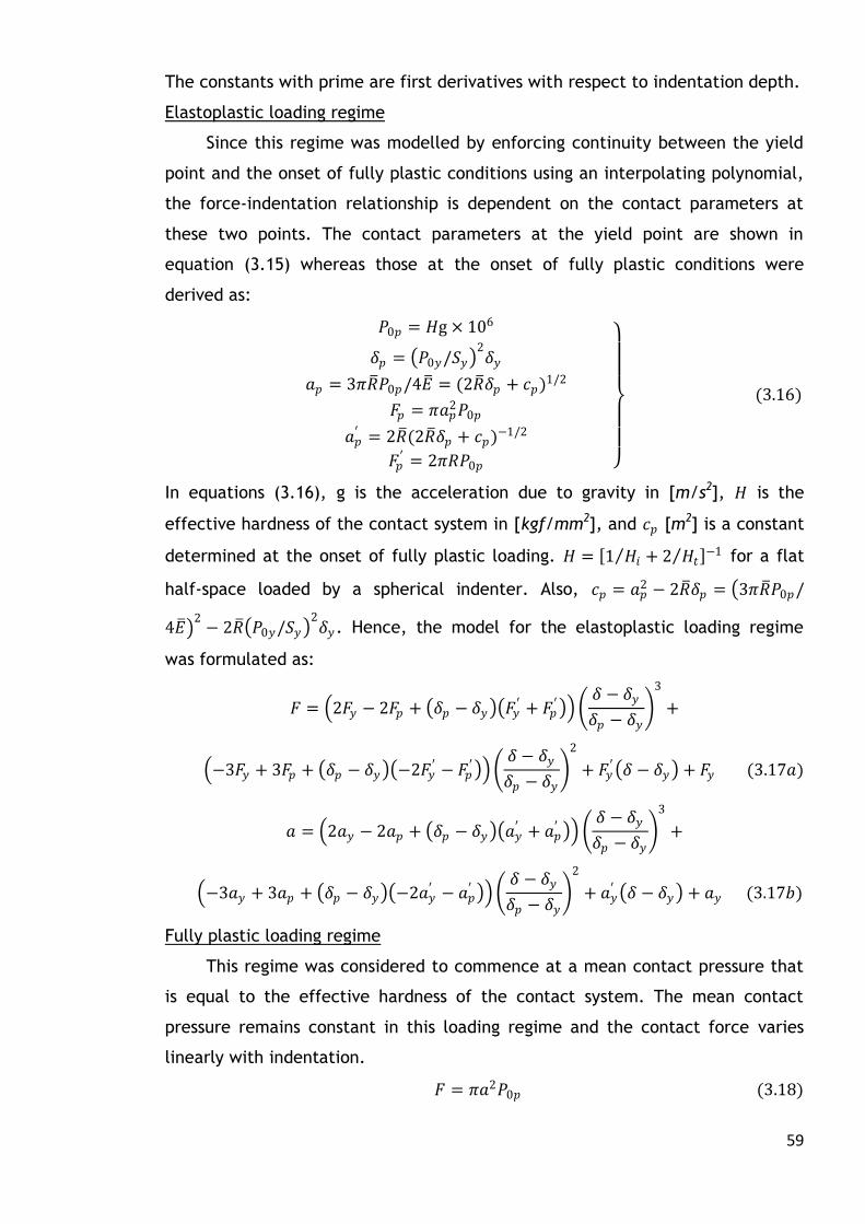
59

The constants with prime are first derivatives with respect to indentation depth.


Since this regime was modelled by enforcing continuity between the yield

point and the onset of fully plastic conditions using an interpolating polynomial,

the force-indentation relationship is dependent on the contact parameters at

these two points. The contact parameters at the yield point are shown in

equation (3.15) whereas those at the onset of fully plastic conditions were

derived as:

𝑃0𝑝 = 𝐻g × 106

𝛿𝑝 = 𝑃0𝑦/𝑆𝑦 2𝛿𝑦

𝑎𝑝 = 3𝜋𝑅 𝑃0𝑝/4𝐸 = (2𝑅 𝛿𝑝 + 𝑐𝑝)1/2

𝐹𝑝 = 𝜋𝑎𝑝2𝑃0𝑝

𝑎𝑝′ = 2𝑅 (2𝑅 𝛿𝑝 + 𝑐𝑝)−1/2

𝐹𝑝′ = 2𝜋𝑅𝑃0𝑝

(3.16)

In equations (3.16), g is the acceleration due to gravity in [m/s2], 𝐻 is the

effective hardness of the contact system in [kgf/mm2], and 𝑐𝑝 [m2] is a constant

determined at the onset of fully plastic loading. 𝐻 = 1 𝐻𝑖 + 2 𝐻𝑡 −1 for a flat

half-space loaded by a spherical indenter. Also, 𝑐𝑝 = 𝑎𝑝2 − 2𝑅 𝛿𝑝 = 3𝜋𝑅 𝑃0𝑝/

4𝐸 2− 2𝑅 𝑃0𝑦/𝑆𝑦

2𝛿𝑦. Hence, the model for the elastoplastic loading regime

was formulated as:

𝐹 = 2𝐹𝑦 − 2𝐹𝑝 + 𝛿𝑝 − 𝛿𝑦 𝐹𝑦′ + 𝐹𝑝

′ 𝛿 − 𝛿𝑦

𝛿𝑝 − 𝛿𝑦

3

+

−3𝐹𝑦 + 3𝐹𝑝 + 𝛿𝑝 − 𝛿𝑦 −2𝐹𝑦′ − 𝐹𝑝

′ 𝛿 − 𝛿𝑦


2

+ 𝐹𝑦′ 𝛿 − 𝛿𝑦 + 𝐹𝑦 (3.17𝑎)

𝑎 = 2𝑎𝑦 − 2𝑎𝑝 + 𝛿𝑝 − 𝛿𝑦 𝑎𝑦′ + 𝑎𝑝

′ 𝛿 − 𝛿𝑦


3

+

−3𝑎𝑦 + 3𝑎𝑝 + 𝛿𝑝 − 𝛿𝑦 −2𝑎𝑦′ − 𝑎𝑝

′ 𝛿 − 𝛿𝑦


2

+ 𝑎𝑦′ 𝛿 − 𝛿𝑦 + 𝑎𝑦 (3.17𝑏)


This regime was considered to commence at a mean contact pressure that

is equal to the effective hardness of the contact system. The mean contact

pressure remains constant in this loading regime and the contact force varies

linearly with indentation.

𝐹 = 𝜋𝑎2𝑃0𝑝 (3.18)

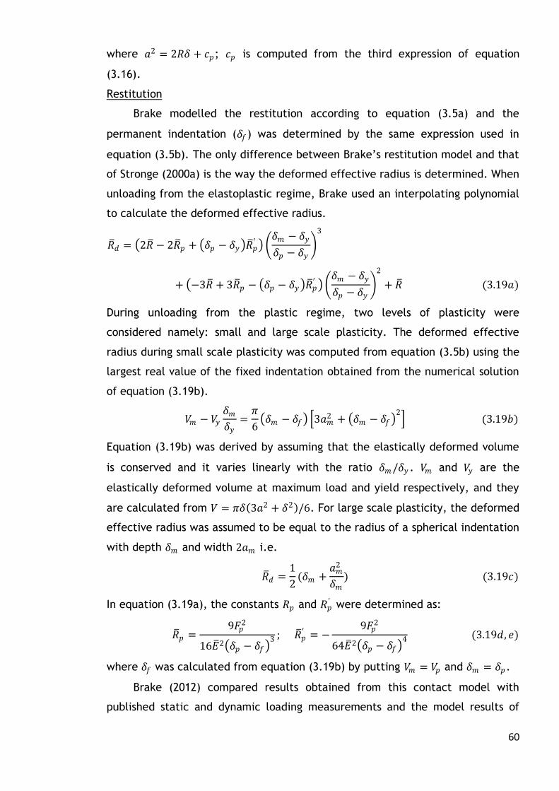
60

where 𝑎2 = 2𝑅𝛿 + 𝑐𝑝; 𝑐𝑝 is computed from the third expression of equation

(3.16).

Restitution

Brake modelled the restitution according to equation (3.5a) and the

permanent indentation (𝛿𝑓) was determined by the same expression used in

equation (3.5b). The only difference between Brake’s restitution model and that

of Stronge (2000a) is the way the deformed effective radius is determined. When

unloading from the elastoplastic regime, Brake used an interpolating polynomial

to calculate the deformed effective radius.

𝑅 𝑑 = 2𝑅 − 2𝑅 𝑝 + 𝛿𝑝 − 𝛿𝑦 𝑅 𝑝′

𝛿𝑚 − 𝛿𝑦


3

+ −3𝑅 + 3𝑅 𝑝 − 𝛿𝑝 − 𝛿𝑦 𝑅 𝑝′

𝛿𝑚 − 𝛿𝑦


2

+ 𝑅 (3.19𝑎)

During unloading from the plastic regime, two levels of plasticity were

considered namely: small and large scale plasticity. The deformed effective

radius during small scale plasticity was computed from equation (3.5b) using the

largest real value of the fixed indentation obtained from the numerical solution

of equation (3.19b).

𝑉𝑚 − 𝑉𝑦𝛿𝑚𝛿𝑦

=𝜋

6 𝛿𝑚 − 𝛿𝑓 3𝑎𝑚

2 + 𝛿𝑚 − 𝛿𝑓 2 (3.19𝑏)

Equation (3.19b) was derived by assuming that the elastically deformed volume

is conserved and it varies linearly with the ratio 𝛿𝑚/𝛿𝑦 . 𝑉𝑚 and 𝑉𝑦 are the

elastically deformed volume at maximum load and yield respectively, and they

are calculated from 𝑉 = 𝜋𝛿 3𝑎2 + 𝛿2 /6. For large scale plasticity, the deformed

effective radius was assumed to be equal to the radius of a spherical indentation

with depth 𝛿𝑚 and width 2𝑎𝑚 i.e.

𝑅 𝑑 =1

2(𝛿𝑚 +

𝑎𝑚2

𝛿𝑚) (3.19𝑐)

In equation (3.19a), the constants 𝑅𝑝 and 𝑅𝑝′ were determined as:

𝑅 𝑝 =9𝐹𝑝

2

16𝐸 2 𝛿𝑝 − 𝛿𝑓 3 ; 𝑅 𝑝

′ = −9𝐹𝑝

2

64𝐸 2 𝛿𝑝 − 𝛿𝑓 4 (3.19𝑑, 𝑒)

where 𝛿𝑓 was calculated from equation (3.19b) by putting 𝑉𝑚 = 𝑉𝑝 and 𝛿𝑚 = 𝛿𝑝.

Brake (2012) compared results obtained from this contact model with

published static and dynamic loading measurements and the model results of

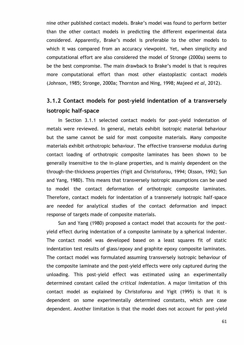
61

nine other published contact models. Brake’s model was found to perform better

than the other contact models in predicting the different experimental data

considered. Apparently, Brake’s model is preferable to the other models to

which it was compared from an accuracy viewpoint. Yet, when simplicity and

computational effort are also considered the model of Stronge (2000a) seems to

be the best compromise. The main drawback to Brake’s model is that is requires

more computational effort than most other elastoplastic contact models

(Johnson, 1985; Stronge, 2000a; Thornton and Ning, 1998; Majeed et al, 2012).

3.1.2 Contact models for post-yield indentation of a transversely

isotropic half-space

In Section 3.1.1 selected contact models for post-yield indentation of

metals were reviewed. In general, metals exhibit isotropic material behaviour

but the same cannot be said for most composite materials. Many composite

materials exhibit orthotropic behaviour. The effective transverse modulus during

contact loading of orthotropic composite laminates has been shown to be

generally insensitive to the in-plane properties, and is mainly dependent on the

through-the-thickness properties (Yigit and Christoforou, 1994; Olsson, 1992; Sun

and Yang, 1980). This means that transversely isotropic assumptions can be used

to model the contact deformation of orthotropic composite laminates.

Therefore, contact models for indentation of a transversely isotropic half-space

are needed for analytical studies of the contact deformation and impact

response of targets made of composite materials.

Sun and Yang (1980) proposed a contact model that accounts for the post-

yield effect during indentation of a composite laminate by a spherical indenter.

The contact model was developed based on a least squares fit of static

indentation test results of glass/epoxy and graphite epoxy composite laminates.

The contact model was formulated assuming transversely isotropic behaviour of

the composite laminate and the post-yield effects were only captured during the

unloading. This post-yield effect was estimated using an experimentally

determined constant called the critical indentation. A major limitation of this

contact model as explained by Christoforou and Yigit (1995) is that it is

dependent on some experimentally determined constants, which are case

dependent. Another limitation is that the model does not account for post-yield

62

effects in the loading stage as it is based on purely elastic loading and therefore,

it is apparent that it would overestimate the maximum contact force during

substantial post-yield deformation. In principle, a purely elastic contact loading

would result in a purely elastic unloading due to complete stress reversal. By the

same reckoning, the presence of post-yield effects in the unloading stage as

confirmed by experiments (Sun and Yang, 1980) implies that the post-yield

effects must first appear in the loading stage.

Post-yield loading of metallic targets give rise to plastic deformation,

whereas the case of composite laminate targets involves both plastic

deformation and damage mechanisms such as fibre breaking/kinking/micro-

buckling and layer delamination (Majeed et al, 2012). Also, the laminate lay-up,

composite weave-style, and the orthotropic behaviour of the composite can

influence the impact response significantly. Accounting for all these factors

would result in very complex models and therefore, simplifying assumptions are

often used. Yigit and Christoforou (1994) developed an elastic-plastic contact

model that accounts for post-yield effects in the loading and unloading stages of

the indentation of a transversely isotropic composite laminate by a spherical

indenter. The model consists of two loading regimes, elastic and elastic-plastic,

and an unloading regime that is considered to be elastic. An advantage of this

contact model is that the contact parameters can be determined from the

material and geometric properties of the contact system. A limitation of the

model is that it could significantly underestimate the maximum contact force

(Majeed et al, 2012).

Majeed et al (2012) developed an elastoplastic contact model that

attempts to improve on the model of Yigit and Christoforou (1994). Following

observations from FE results for the post-yield indentation of a half-space,

Majeed et al (2012) suggested that the transition to the elastoplastic loading

regime occurs at a mean pressure equal to the arithmetic average of the mean

pressure at yield and at the onset of fully plastic conditions, i.e. 1.95𝑆𝑦 . Based

on this idea, Majeed et al (2012) formulated a contact model consisting of two

loading regimes, elastic and elastic-plastic, and one unloading regime. The

elastic loading regime was modelled using the Hertz contact model and assumed

to terminate at a transition mean pressure of 1.95𝑆𝑦 . The elastic-plastic loading

regime was modelled using the perfectly-plastic assumption of a constant mean

63

pressure that was considered to be equal to the transition mean pressure. Post-

yield effects were captured in the elastic-plastic loading regime and the

unloading regime. The model of Majeed et al (2012) is summarised as follows.


𝐹 = 𝐾𝑕𝛿3 2 0 ≤ 𝛿 ≤ 𝛿𝑝 (3.20)

where 𝐾𝑕 = 4/3 𝐸 𝑅 1/2; 𝐸 and 𝑅 are the effective modulus and radius of the

contact or impact system. 𝑅 has the same definition as in equation (3.1) while 𝐸

is defined for a spherical indenter in contact with a transversely isotropic target

as:

𝐸 = 1 − 𝜐𝑖2 𝐸𝑖 + 1 𝐸𝑡 −1 (3.21)

𝐸𝑡 is the effective modulus of the transversely isotropic target and could be

estimated as 𝐸𝑡 = 2/𝑐1𝑐3 (Turner, 1980), where 𝑐1 and 𝑐3 are constant given by

𝑐1 = 𝐸𝑥/𝐸𝑧 − 𝜐𝑥𝑧2

1 − 𝜐𝑥𝑦2; 𝑐2 =

𝐸𝑥/2𝐺𝑥𝑧 − 𝜐𝑥𝑧 1 + 𝜐𝑥𝑦

1 − 𝜐𝑥𝑦2; 𝑐3 =

1 − 𝜐𝑥𝑦

2𝐺𝑥𝑦 𝑐1 + 𝑐2

2

𝑥 and 𝑦 represent the in-plane directions while 𝑧 represents the thickness

direction. 𝐺𝑥𝑧 and 𝐺𝑥𝑦 are shear moduli acting in the planes indicated by their

subscripts, and 𝜐𝑥𝑧 and 𝜐𝑥𝑦 are the corresponding Poisson’s ratios. The subscripts

1, 2, and 3 are only used to distinguish the constants and do not have any

directional significance.

Another expression for estimating 𝐸𝑡 is (Olsson, 1992)

1

𝐸𝑡=

1 − 𝜐𝑥𝑧𝜐𝑧𝑥𝐸𝑧

(3.22)

For most composite laminates the product 𝜐𝑥𝑧𝜐𝑧𝑥 ≅ 0 (Olsson, 1992). Therefore,

the effective modulus of a transversely isotropic laminate is approximately equal

to the transverse modulus of its ply i.e. 𝐸𝑡 ≅ 𝐸𝑧 = 𝐸33. Note that 𝐸33 ≅ 𝐸22 for

most composite laminates. This approximation has been used with excellent

success in many impact studies involving composite laminates (Yang and Sun,

1980; Olsson, 1992; Wu and Shyu, 1993; Yigit and Christoforou, 1994; Carvalho

and Guedes Soares, 1996).

The indentation at the end of the elastic loading regime was derived as:

𝛿𝑝 =9𝜋2𝑘2𝑆𝑦

2𝑅

16𝐸 2; 𝑘 = 1.95 (3.33)


𝐹 = 𝐾𝑝 𝛿 − 𝛿𝑝 + 𝐾𝑕𝛿𝑝3 2 𝛿𝑝 ≤ 𝛿 ≤ 𝛿𝑚 (3.24)

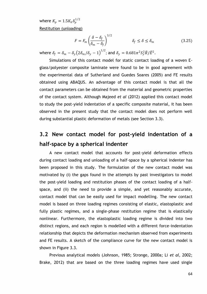
64

where 𝐾𝑝 = 1.5𝐾𝑕𝛿𝑝1 2

Restitution (unloading)

𝐹 = 𝐹𝑚 𝛿 − 𝛿𝑓

𝛿𝑚 − 𝛿𝑓

3 2

𝛿𝑓 ≤ 𝛿 ≤ 𝛿𝑚 (3.25)

where 𝛿𝑓 = 𝛿𝑚 − 𝛿𝑦 2𝛿𝑚/𝛿𝑦 − 1 1/2

; and 𝛿𝑦 = 0.681𝜋2𝑆𝑦2𝑅 /𝐸 2.

Simulations of this contact model for static contact loading of a woven E-

glass/polyester composite laminate were found to be in good agreement with

the experimental data of Sutherland and Guedes Soares (2005) and FE results

obtained using ABAQUS. An advantage of this contact model is that all the

contact parameters can be obtained from the material and geometric properties

of the contact system. Although Majeed et al (2012) applied this contact model

to study the post-yield indentation of a specific composite material, it has been

observed in the present study that the contact model does not perform well

during substantial plastic deformation of metals (see Section 3.3).

3.2 New contact model for post-yield indentation of a

half-space by a spherical indenter

A new contact model that accounts for post-yield deformation effects

during contact loading and unloading of a half-space by a spherical indenter has

been proposed in this study. The formulation of the new contact model was

motivated by (i) the gaps found in the attempts by past investigators to model

the post-yield loading and restitution phases of the contact loading of a half-

space, and (ii) the need to provide a simple, and yet reasonably accurate,

contact model that can be easily used for impact modelling. The new contact

model is based on three loading regimes consisting of elastic, elastoplastic and

fully plastic regimes, and a single-phase restitution regime that is elastically

nonlinear. Furthermore, the elastoplastic loading regime is divided into two

distinct regions, and each region is modelled with a different force-indentation

relationship that depicts the deformation mechanism observed from experiments

and FE results. A sketch of the compliance curve for the new contact model is

shown in Figure 3.3.

Previous analytical models (Johnson, 1985; Stronge, 2000a; Li et al, 2002;

Brake, 2012) that are based on the three loading regimes have used single

65

𝛿𝑡𝑒𝑝 𝛿

𝛿𝑚 𝛿𝑝 𝛿𝑓 𝛿𝑦 𝛿𝑟

A

Elastoplastic Fully plastic Elastic

Region I Region II

B

C

D

E

0

𝐹

continuous functions to model the elastoplastic loading regime. However,

experimental evidence and FE results reveal that there is a linear loading region

preceding the onset of fully plastic loading predicted by indentation theory

(Majeed et al, 2012). Also, indentation theory and experimental evidence reveal

that a nonlinear loading exists in the elastoplastic regime (Majeed et al, 2012).

Therefore, it is proposed here that the elastoplastic loading regime can be

divided into two regions as follows:

Figure 3.3: Sketch of compliance curve for the new contact law.

a. Region I: this is characterised by a nonlinear force-indentation relationship.

The onset of this region is the yield point and it ends somewhere in the

elastoplastic regime. In this region, the plastically-deformed material is well

below the contact surface and it is smaller in comparison with the

surrounding elastically-deformed material (Figure 3.4a). This means that the

plastically-deformed material is fully contained within the surrounding

elastic material and the indenter is only in contact with the elastically-

deformed material.

b. Region II: this is characterised by a linear force-indentation relationship. The

region commences from the terminus of region I and ends at the onset of

fully plastic conditions. Here, the plastically-deformed material is

66

(a) (b)

δ

a

0.4

5a

R

δ

a

0.4

5a

R

considered to be comparable or larger in volume than the surrounding

elastically-deformed material (Figure 3.4b). The plastically-deformed

material grows closer to the contact surface, and breaks free to the contact

surface at the end of this region.

In the present study, it is proposed that region I can be modelled by a

modified form of the Hertz contact law that incorporates a yield effect. This

region is modelled in this way since it has similar characteristics as the elastic

loading regime namely: (i) it is nonlinear and (ii) its deformation can be

considered to be effectively elastic-like since the plastically-deformed material

is small and fully contained within the surrounding elastically-deformed

material. Region II is modelled using a linear force-indentation that incorporates

the appropriate plastic deformation effect, which is assumed to occur at

transition point in the elastoplastic loading regime.

Figure 3.4: Plastic deformation in the elastoplastic loading regime (a) during

nonlinear elastoplastic deformation (b) during linear elastoplastic deformation.

The cross-hatched area is the surrounding elastically-deformed material while

the unshaded area is the plastically-deformed material.

The features of these two regions can be seen in the approximate

analytical models for the elastoplastic loading regime presented in (Johnson,

1985; Stronge, 2000a). These models incorporate plastic deformation effects and

the nonlinear part of the elastoplastic loading appears as a logarithmic function

of the indentation. The existence of the two regions in the elastoplastic loading

regimes means that there is a transition point from region I to region II. Majeed

et al (2012) assumed that the transition from region I to region II occurs at the

point where the mean contact pressure is equal to the arithmetic average of the

mean contact pressures at yield and at fully plastic conditions i.e. the transition

67

occurs at 𝑃0 = 1.95𝑆𝑦 . Although this assumption produced results that are

supported by the static indentation experiments of woven E-glass/polyester

composite laminate, it requires further validation. In the proposed analysis the

indentation and mean contact pressure at the transition point are derived

analytically from continuity conditions and existing indentation theory.

Based on the foregoing discussions, the following force-indentation

relationships are proposed for modelling the static loading and unloading of a

half-space target by a spherical indenter.


𝐹𝑒 = 𝐾𝑕𝛿3 2 0 ≤ 𝛿 ≤ 𝛿𝑦 (3.26)


Region I: Nonlinear elastoplastic loading

𝐹𝑒𝑝𝐼 = 𝐾𝑕 𝛿 − 𝛿𝑦

3 2 + 𝐾𝑕𝛿𝑦

3 2 𝛿𝑦 ≤ 𝛿 ≤ 𝛿𝑡𝑒𝑝 (3.27)

Region II: Linear elastoplastic loading

𝐹𝑒𝑝𝐼𝐼 = 𝐾𝑙 𝛿 − 𝛿𝑡𝑒𝑝 + 𝐾𝑕 𝛿𝑡𝑒𝑝 − 𝛿𝑦

3 2 + 𝛿𝑦

3 2 𝛿𝑡𝑒𝑝 ≤ 𝛿 ≤ 𝛿𝑝 (3.28)


𝐹𝑓𝑝 = 𝐾𝑝 𝛿 − 𝛿𝑝 + 𝐹𝛿=𝛿𝑝 𝛿𝑝 ≤ 𝛿 ≤ 𝛿𝑚 (3.29)


𝐹𝑢 = 𝐾𝑢 𝛿 − 𝛿𝑓 3 2

𝛿𝑓 ≤ 𝛿 ≤ 𝛿𝑚 (3.30)

where 𝐹𝑒, 𝐹𝑒𝑝 , 𝐹𝑓𝑝 , and 𝐹𝑢 are the elastic, elastoplastic, fully plastic, and

unloading forces respectively. The superscripts on 𝐹𝑒𝑝 indicate the region in the

elastoplastic regime, and 𝐹𝛿=𝛿𝑝 is the value of the contact force at the onset of

fully plastic conditions. 𝐾𝑕 is the Hertzian contact stiffness, 𝐾𝑙 is the linear

stiffness in region II, 𝐾𝑝 is the linear stiffness during the fully plastic loading

regime and 𝐾𝑢 is the nonlinear stiffness during unloading. 𝛿𝑦 is the indentation

at yield, 𝛿𝑡𝑒𝑝 is the indentation at the transition between region I and region II,

𝛿𝑝 is the indentation at the onset of fully plastic conditions and 𝛿𝑓 is the fixed or

permanent or non-recoverable indentation. The contact parameters in the

model are derived next.

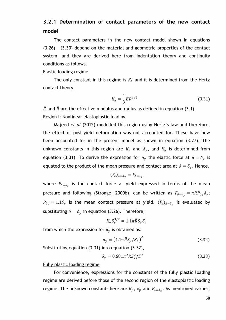
68

3.2.1 Determination of contact parameters of the new contact

model

The contact parameters in the new contact model shown in equations

(3.26) – (3.30) depend on the material and geometric properties of the contact

system, and they are derived here from indentation theory and continuity

conditions as follows.


The only constant in this regime is 𝐾𝑕 and it is determined from the Hertz

contact theory.

𝐾𝑕 =4

3𝐸 𝑅 1 2 (3.31)

𝐸 and 𝑅 are the effective modulus and radius as defined in equation (3.1).


Majeed et al (2012) modelled this region using Hertz’s law and therefore,

the effect of post-yield deformation was not accounted for. These have now

been accounted for in the present model as shown in equation (3.27). The

unknown constants in this region are 𝐾𝑕 and 𝛿𝑦 , and 𝐾𝑕 is determined from

equation (3.31). To derive the expression for 𝛿𝑦 the elastic force at 𝛿 = 𝛿𝑦 is

equated to the product of the mean pressure and contact area at 𝛿 = 𝛿𝑦 . Hence,

𝐹𝑒 𝛿=𝛿𝑦 = 𝐹𝛿=𝛿𝑦

where 𝐹𝛿=𝛿𝑦 is the contact force at yield expressed in terms of the mean

pressure and following (Stronge, 2000b), can be written as 𝐹𝛿=𝛿𝑦 = 𝜋𝑅 𝑃0𝑦𝛿𝑦;

𝑃0𝑦 = 1.1𝑆𝑦 is the mean contact pressure at yield. 𝐹𝑒 𝛿=𝛿𝑦 is evaluated by

substituting 𝛿 = 𝛿𝑦 in equation (3.26). Therefore,

𝐾𝑕𝛿𝑦3 2 = 1.1𝜋𝑅 𝑆𝑦𝛿𝑦

from which the expression for 𝛿𝑦 is obtained as:

𝛿𝑦 = 1.1𝜋𝑅 𝑆𝑦/𝐾𝑕 2

(3.32)

Substituting equation (3.31) into equation (3.32),

𝛿𝑦 = 0.681𝜋2𝑅 𝑆𝑦2/𝐸 2 (3.33)


For convenience, expressions for the constants of the fully plastic loading

regime are derived before those of the second region of the elastoplastic loading

regime. The unknown constants here are 𝐾𝑝, 𝛿𝑝 and 𝐹𝛿=𝛿𝑝 . As mentioned earlier,

69

the mean pressure in this regime is constant and therefore, the contact force at

any point in this regime can be written as:

𝐹𝑓𝑝 = 𝜋𝑃0𝑝𝑎2 (3.34)

where 𝑃0𝑝 = 2.8𝑆𝑦 is the mean contact pressure at fully plastic conditions and 𝑎

is the contact radius. Since the force-indentation relationship in this loading

regime is linear, 𝑎2 ∝ 𝛿. A general relationship between the contact radius and

indentation can be written as 𝑎2 = 2𝑅 𝛿 + 𝑐𝑝 where the constant 𝑐𝑝 = 𝑎𝑝2 −

2𝑅 𝛿𝑝 ≠ 0 can be either positive of negative depending on the values of 𝑎𝑝 and 𝛿𝑝

(Brake, 2012). Therefore,

𝑎2 = 2𝑅 (𝛿 − 𝛿𝑝) + 𝑎𝑝2 3.35

Substituting equation (3.35) in equation (3.34) and comparing the resulting

expression with equation (3.29), it can be deduced that

𝐾𝑝 = 5.6𝜋𝑅 𝑆𝑦 (3.36𝑎)

and

𝐹𝛿=𝛿𝑝 = 𝜋𝑃0𝑝𝑎𝑝2 = 2.8𝜋𝑆𝑦𝑎𝑝

2 (3.36𝑏)

where 𝑎𝑝 can be determined according to Stronge (2000a) as: 𝑎𝑝2 = 𝑅 (2𝛿𝑝 − 𝛿𝑦).

Equation (3.36a) represents the case of a perfectly rigid indenter in contact with

a perfectly plastic half-space. When equation (3.36a) was used in the simulation

of the force-indentation curve for selected experimental cases (Alcalá et al,

1998; Bartier et al, 2010) the contact force predictions obtained during the fully

plastic loading regime were significantly higher than the experimental data to

which the predictions were compared. This is because the hardness of the

indenters used in the experiments is just a few times higher than the hardness of

the indented surfaces and therefore, the indenters cannot be considered to be

perfectly rigid. Brake (2012) proposed an effective hardness to account for the

effect of the relative hardness. For a spherical indenter in contact with a

compliant flat surface, Brake (2012) determined the effective hardness as

𝐻 = 1 𝐻𝑖 + 2 𝐻𝑡 −1 where 𝑆𝑦 < 𝐻 < 2.8𝑆𝑦 . Using this effective hardness a factor

accounting for the relative hardness effect is introduced in the present model

as: 휂 = 𝐻/ 2.8𝑆𝑦 = 1 𝐻𝑖 + 2 𝐻𝑡 −1/ 2.8𝑆𝑦 . Hence,

𝐾𝑝 = 5.6𝜋휂𝑅 𝑆𝑦 (3.37)

For the experiments of Alcalá et al (1998) and Bartier et al (2010) the factor was

calculated as 휂 = 0.81 and 휂 = 0.85 respectively. An average value of 휂𝑎𝑣 = 0.83

70

was used in equation (3.37) and found to give good predictions of the

experimental data. Consequently, the constant 𝐾𝑝 is has been calculated as:

𝐾𝑝 = 4.65𝜋𝑅 𝑆𝑦 (3.38)

If 𝐻𝑖 𝐻𝑡 ≥ 100 then 휂 ≅ 1, and the indenter can be considered to be rigid so that

equation (3.36a) can be used to calculate 𝐾𝑝. In cases where hardness data is

unavailable equation (3.38) can be used to calculate 𝐾𝑝 otherwise equation

(3.37) is used. Note that the value of 𝐾𝑝 does not affect the elastoplastic

response; but it determines the fully plastic response.

To evaluate completely the contact force in the fully plastic loading

regime, the value or expression for 𝛿𝑝 or 𝛿𝑝/𝛿𝑦 must be known. In the literature,

different expressions have been used for the ratio 𝛿𝑝/𝛿𝑦 . Brake (2012) used the

expression 𝛿𝑝/𝛿𝑦 = (𝑃𝑜𝑝/𝑆𝑦)2 = 7.84 where 𝑃𝑜𝑝 = 2.8𝑆𝑦. This expression is the von

Mises equivalent of the expression given by Stronge (2000b) that is based on

Tresca’s yield criterion. Brake (2012) observed that the use of this expression

sometimes produces an unrealistic bend in the elastoplastic regime and a

smoothing condition was applied to correct this. The condition states that the

slope of the contact force at 𝛿 = 𝛿𝑝 is equal to the slope of the extended

Hertzian force at the same indentation i.e. 𝑑𝐹𝑒 𝑑𝛿 𝛿=𝛿𝑝 = 𝑑𝐹𝑓𝑝 𝑑𝛿 𝛿=𝛿𝑝

. Using

equations (3.26) and (3.34), and 𝛿𝑦 = (𝜋𝑅 𝑃𝑜𝑦 /𝐾𝑕)2 in the smoothing condition,

the resulting ratio is 𝛿𝑝/𝛿𝑦 = (4𝑃𝑜𝑝/3𝑃𝑜𝑦 )2 = 13.94 where 𝑃𝑜𝑦 = 𝑆𝑦 has been used

in-line with the von Mises yield criterion. Stronge (2000a) presented an

approximate analytical formula that expresses the normalised mean pressure in

the elastoplastic loading regime as a function of the normalised indentation.

Evaluating this formula at 𝛿 = 𝛿𝑝 results in 𝛿𝑝/𝛿𝑦 = 82.5, which translates into a

force ratio of 𝐹𝑝/𝐹𝑦 = 417.5. Johnson (1985) gave a force ratio of 𝐹𝑝/𝐹𝑦 ≈ 400,

and based on Johnson’s model for the fully plastic loading regime a ratio of

𝛿𝑝/𝛿𝑦 ≈ 73 can be obtained. Stronge (2000a) also reported a ratio of 𝛿𝑝/𝛿𝑦 ≈

140 and a corresponding force ratio of 𝐹𝑝/𝐹𝑦 ≈ 650 from finite element studies

of elastic-perfectly plastic bodies. The results of Johnson (1985) and Stronge

(2000a) are close and are based on theoretically valid analytical approximations

of the elastoplastic loading regime. Therefore, a ratio of 𝛿𝑝/𝛿𝑦 = 82.5 has been

used in the present study. However, parametric studies based on the formulation

71

of the elastoplastic regime of the new contact model reveal that 𝛿𝑝/𝛿𝑦 can be

reasonably varied from 28 to 140 as shown in later discussions in this chapter.

Hence,

𝛿𝑝 = 82.5𝛿𝑦 = 56.18𝜋2𝑅 𝑆𝑦2/𝐸 2 (3.39)


In this region, two constants are to be determined; 𝐾𝑙 and 𝛿𝑡𝑒𝑝 . To obtain

expressions for these constants, the following continuity conditions are applied.

Condition 1: The slope of region II is equal to the slope of region I at 𝛿 = 𝛿𝑡𝑒𝑝 .

The condition implies that the linear stiffness of region II is equal to the slope of

region I at 𝛿 = 𝛿𝑡𝑒𝑝 . This condition has been used by Yigit and Christoforou

(1994) and Majeed et al (2012) when considering transition from a nonlinear

behaviour to a linear behaviour. It is dimensionally consistent, and therefore has

also been applied in the present modelling. The condition can be expressed

mathematically as:

𝑑𝐹𝑒𝑝

𝐼𝐼

𝑑𝛿 𝛿=𝛿𝑡𝑒𝑝

= 𝑑𝐹𝑒𝑝

𝐼

𝑑𝛿 𝛿=𝛿𝑡𝑒𝑝

from which we get:

𝐾𝑙 = 1.5𝐾𝑕 𝛿𝑡𝑒𝑝 − 𝛿𝑦 1 2

(3.40)

Condition 2: The value of the linear elastoplastic force is equal to the value of

the fully plastic force at 𝛿 = 𝛿𝑝 .

𝐹𝑒𝑝𝐼𝐼

𝛿=𝛿𝑝= 𝐹𝑓𝑝 𝛿=𝛿𝑝

Substituting equations (3.29) and (3.40) into this condition,

𝐾𝑙 𝛿𝑝 − 𝛿𝑡𝑒𝑝 + 𝐾𝑕 𝛿𝑡𝑒𝑝 − 𝛿𝑦 3 2

+ 𝛿𝑦3 2 = 𝐹𝛿=𝛿𝑝 (3.41)

From equation (3.41), 𝐾𝑙 can be expressed as:

𝐾𝑙 =𝐹𝛿=𝛿𝑝 − 𝐾𝑕 𝛿𝑡𝑒𝑝 − 𝛿𝑦

3 2 + 𝛿𝑦

3 2

𝛿𝑝 − 𝛿𝑡𝑒𝑝 (3.42)

Using equations (3.40) and (3.42), the following nonlinear equation can be

obtained.

𝐾𝑕 𝛿𝑡𝑒𝑝 − 𝛿𝑦 3 2

− 1.5𝐾𝑕 𝛿𝑡𝑒𝑝 − 𝛿𝑦 1 2

𝛿𝑡𝑒𝑝 − 𝛿𝑝 = 𝐹𝛿=𝛿𝑝 − 𝐾𝑕𝛿𝑦3 2 (3.43)

Squaring both sides of equation (3.43) and after some algebraic simplifications

(see appendix A.1), a cubic equation in 𝛿𝑡𝑒𝑝 is obtained as shown in equation

(3.44).

72

𝛿𝑡𝑒𝑝3 − Λ1𝛿𝑡𝑒𝑝

2 + Λ2𝛿𝑡𝑒𝑝 − Λ3 = 0 (3.44)

Λ1 = 6𝛿𝑝 − 3𝛿𝑦 ; Λ2 = 9𝛿𝑝2 − 6𝛿𝑦𝛿𝑝; Λ3 = 4𝛿𝑦

3 − 12𝛿𝑦2𝛿𝑝 + 9𝛿𝑦𝛿𝑝

2 + 2𝑍 𝐾𝑕 2; and

𝑍 = 𝐹𝛿=𝛿𝑝 − 𝐾𝑕𝛿𝑦3 2

. The value of 𝛿𝑡𝑒𝑝 obtained from equation (3.44) is

substituted into equation (3.40) to calculate the value of 𝐾𝑙. The solution to

equation (3.44) must be within the range 𝛿𝑦 < 𝛿𝑡𝑒𝑝 < 𝛿𝑝.


There are two unknown constants in this regime according to equation

(3.30). The constants are the unloading stiffness 𝐾𝑢 and the non-recoverable

indentation 𝛿𝑓. In order to determine the expressions for these constants, two

new variables are needed namely: the maximum indentation 𝛿𝑚 and the

maximum contact force 𝐹𝑚 . Since this phase is elastic, the force-indentation

relationship is analogous to the Hertz contact model for elastic loading. The

constants are determined using the same expressions as used by Stronge (2000a):

𝐾𝑢 =4

3𝐸 𝑅 𝑑

1 2 (3.45𝑎)

𝛿𝑓 = 𝛿𝑚 − 3𝐹𝑚

4𝐸 𝑅 𝑑1 2

2 3

(3.45𝑏)

where 𝑅 𝑑 is the deformed effective radius, and 𝑅 𝑑 ≥ 𝑅 . Whereas the Hertz

stiffness is related to the effective radius, the unloading stiffness is related to a

deformed effective radius due to plastic deformation effects (Stronge, 2000a).

The main difference between the present restitution model and that of

Stronge (2000a) is in the way 𝑅 𝑑 is determined. Following suggestions of Johnson

(1985) and Brake (2012), Big-Alabo et al (2014a; 2015a) determined 𝑅 𝑑 as

follows: 𝑅 𝑑 ≅ 𝑅 when the maximum penetration is in the elastoplastic loading

regime or the initial phase of the fully plastic loading regime; and 𝑅 𝑑 ≅ 𝑅 + 𝛿𝑚/2

when the maximum penetration is well into the fully plastic loading regime. The

approximations used by Big-Alabo et al (2014a; 2015a) could lead to significant

underestimation of the permanent indentation at the end of the unloading (Big-

Alabo et al, 2015a). Johnson (1985) stated that 𝑅 𝑑 ≅ 2.0𝑅 when unloading from

the onset of fully plastic conditions if piling and sinking are neglected. Based on

FE results of the indentation of an elastic-perfectly plastic material, Li et al

(2002) determined the value of 𝑅 𝑑 when unloading from the onset of fully plastic

indentation as 𝑅 𝑑 ≅ 2.15𝑅 . Hill et al (1989) reported that 𝑅 𝑑 could reach a value

of 2.8𝑅 during indentation of perfectly plastic materials. Hence, it could be said

73

that 𝑅 𝑑 lies in the range of 𝑅 ≤ 𝑅 𝑑 ≤ 2.8𝑅 during post-yield unloading. Since the

present contact model consists of a linear elastoplastic loading regime that

exhibits an indentation behaviour that is much like that of the fully plastic

loading regime, it is assumed that Johnson’s suggestion of 𝑅 𝑑 ≅ 2.0𝑅 occurs

when unloading from the onset of the linear elastoplastic loading. This means

that 𝑅 𝑑 varies between 𝑅 and 2.0𝑅 during unloading from the nonlinear

elastoplastic loading regime i.e. 𝛿𝑦 ≤ 𝛿𝑚 ≤ 𝛿𝑡𝑒𝑝 . Also, based on the observation

of Hill et al (1989) and to ensure continuity, 𝑅 𝑑 is assumed to vary between 2.0𝑅

and 2.8𝑅 during unloading from the linear elastoplastic loading regime i.e.

𝛿𝑡𝑒𝑝 ≤ 𝛿𝑚 ≤ 𝛿𝑝. Finite element studies conducted by Li et al (2002) on the

variation of 𝑅 𝑑 with indentation revealed that 𝑅 𝑑 is approximately constant once

fully plastic conditions are reached. Here, 𝑅 𝑑 is assumed to have a constant

value of 2.8𝑅 when unloading from the fully plastic loading regime. Therefore,

the following expressions have been used to calculate 𝑅 𝑑.

𝑅 𝑑 = 𝑅 0 ≤ 𝛿𝑚 ≤ 𝛿𝑦

𝑅 𝑑 = 𝛿𝑚 − 𝛿𝑦

𝛿𝑡𝑒𝑝 − 𝛿𝑦

3/2

+ 1 𝑅 𝛿𝑦 ≤ 𝛿𝑚 ≤ 𝛿𝑡𝑒𝑝

𝑅 𝑑 = 0.8 𝛿𝑚 − 𝛿𝑡𝑒𝑝

𝛿𝑝 − 𝛿𝑡𝑒𝑝 + 2 𝑅 𝛿𝑡𝑒𝑝 ≤ 𝛿𝑚 ≤ 𝛿𝑝

𝑅 𝑑 = 2.8𝑅 𝛿𝑚 > 𝛿𝑝

(3.46)

3.2.2 Normalised form of new contact model

In this section, the contact model presented in equations (3.26) to (3.30) is

normalised with respect to the contact force at yield. The normalised contact

model is more elegant and easier to compute. Dividing equations (3.26) to (3.30)

by 𝐹𝑦 = 𝐾𝑕𝛿𝑦3 2

, the normalised form of the present contact model is derived as

shown:


𝐹 𝑒 = 𝛿 3 2 0 ≤ 𝛿 ≤ 1 (3.47)



𝐹 𝑒𝑝𝐼 = 𝛿 − 1

3 2 + 1 1 ≤ 𝛿 ≤ 𝛿 𝑡𝑒𝑝 (3.48)


𝐹 𝑒𝑝𝐼𝐼 = 1.5 𝛿 𝑡𝑒𝑝 − 1

1 2 𝛿 − 𝛿 𝑡𝑒𝑝 + 𝛿 𝑡𝑒𝑝 − 1

3 2 + 1 𝛿 𝑡𝑒𝑝 ≤ 𝛿 ≤ 𝛿 𝑝 (3.49)

74


𝐹 𝑓𝑝 = 4.182 𝛿 − 𝛿 𝑝 + 2.545 2𝛿 𝑝 − 1 𝛿 𝑝 ≤ 𝛿 ≤ 𝛿 𝑚 (3.50)


𝐹 𝑢 = 𝐾 𝑢 𝛿 − 𝛿 𝑓 3 2

𝛿 𝑓 ≤ 𝛿 ≤ 𝛿 𝑚 (3.51)

In equations (3.47) to (3.51), the bar over the forces indicate normalisation with

respect to 𝐹𝑦 and the bar over the indentations indicate normalisation with

respect to 𝛿𝑦 e.g. 𝐹 𝑒 = 𝐹𝑒/𝐹𝑦 and 𝛿 = 𝛿/𝛿𝑦 . The constant 𝛿 𝑡𝑒𝑝 lies within the

range 1 < 𝛿 𝑡𝑒𝑝 < 𝛿 𝑝, and is obtained from

𝛿 𝑡𝑒𝑝3 − Ω1𝛿 𝑡𝑒𝑝

2 + Ω2𝛿 𝑡𝑒𝑝 − Ω3 = 0 (3.52)

Ω1 = 6𝛿 𝑝 − 3; Ω2 = 9𝛿 𝑝2 − 6𝛿 𝑝; and Ω3 = 54.268 − 156.352𝛿 𝑝 + 112.632𝛿 𝑝

2. Also,

𝛿 𝑝 = 82.5; 𝐾 𝑢 = 𝑅 𝑑/𝑅 and 𝛿 𝑓 = 𝛿 𝑚 − 3𝐹𝑚/4𝐸 𝑅 𝑑1 2

2 3 /𝛿𝑦. Equation (3.52) can be

derived by dividing equation (3.44) by 𝛿𝑦3, or solving equations (3.49) and (3.50)

simultaneously at 𝛿 = 𝛿 𝑝. Given that all the coefficients of the cubic equation in

𝛿 𝑡𝑒𝑝 are dependent on 𝛿 𝑝, then substituting 𝛿 𝑝 = 82.5 and solving equation (3.52)

gives 𝛿 𝑡𝑒𝑝 = 13.93.

3.3 Validation of new contact model

The new contact model formulated above was validated by comparing its

results with published experimental data for both static and dynamic indentation

cases. Static indention is one in which the initial velocity of the indenter is zero,

while dynamic indentation involves an initial velocity greater than zero. For the

static indentation analysis the experiments of Alcalá et al (1998) and Bartier et

al (2010) were used for validation; while for the dynamic indentation analysis

the coefficient of restitution measurements by Mok and Duffy (1965) and Kharaz

and Gorham (2000) were used for validation.

3.3.1 Some observations of the new contact model

To understand the features and workings of the new contact model and to

compare with the findings of published analytical models and experimental data,

parametric studies were carried out on the present model.

Using Brake’s contact model, it was shown that the smoothed formulation

for the elastoplastic loading regime always produced the best result and

75

𝛿 𝑝 = 13.94 according to the smoothed formulation. In the current model, the

transition point in the elastoplastic loading regime was found to occur at

𝛿 𝑡𝑒𝑝 = 13.93. This point coincides with the point at which Brake’s smoothed

formulation assumes a transition to the fully plastic regime. The implication is

that a transition from nonlinear to linear deformation behaviour occurs at this

point. Whereas Brake’s model suggests that this point (i.e. 𝛿 ≅ 13.93) marks the

onset of fully plastic conditions, the present model indicates that the point is

located within the elastoplastic loading regime and gives rise to a linear

elastoplastic deformation just before fully plastic conditions are reached. The

presence of linear elastoplastic deformation behaviour during contact loading

has been reported (Majeed et al, 2012) and can also be seen in the compliance

curve for elastoplastic indentation presented by Johnson (1985).

When 𝛿 𝑡𝑒𝑝 = 13.93 is substituted into equation (3.49), the normalised force

at the transition point in the elastoplastic loading regime is calculated to be

𝐹 𝑡𝑒𝑝 = 47.5. According to Stronge (2000a), the normalised contact force in the

elastoplastic loading regime can be expressed in terms of the normalised mean

pressure and indentation as: 𝐹/𝐹𝑦 = 𝑃0/𝑃0𝑦 2𝛿/𝛿𝑦 − 1 . Putting 𝛿 𝑡𝑒𝑝 = 13.93,

𝐹 𝑡𝑒𝑝 = 47.5, and noting that 𝑃𝑜𝑦 = 1.1𝑆𝑦, the mean pressure at 𝛿 = 𝛿 𝑡𝑒𝑝 was

calculated to be equal to 1.945𝑆𝑦 . This value, which is approximately equal to

1.95𝑆𝑦 , is in agreement with the transition mean pressure in the elastoplastic

loading regime proposed by Majeed et al (2012). However, according to Majeed

et al (2012) the transition mean pressure occurs when 𝛿 ≅ 3.15, whereas for the

present model it occurs at 𝛿 = 13.93. In agreement with Brake’s model the

present contact model confirms that the contact deformation changes from

nonlinear to linear behaviour when the normalised indentation is equal to 13.94;

and in agreement with the model of Majeed et al (2012) the present contact

model confirms that the contact deformation in the elastoplastic loading regime

changes from nonlinear to linear behaviour at a mean pressure of 1.95𝑆𝑦 . Since

the non-dimensional indentation of 13.94 and the mean pressure of 1.95𝑆𝑦 occur

at the same point according to the present model, it appears that these values

are unique constants for the transition point in the elastoplastic loading regime.

The transition point in the elastoplastic loading regime of the current

model lies in the range 1 < 𝛿 𝑡𝑒𝑝 < 𝛿 𝑝, and this transition point is determined

76

from the cubic equation that was derived from continuity conditions. In a

limiting case, 𝛿 𝑡𝑒𝑝 will be equal to 𝛿 𝑝, but it is not possible for 𝛿 𝑡𝑒𝑝 to be greater

than 𝛿 𝑝. Using these practical restrictions, the possible range of applicable

values for 𝛿 𝑡𝑒𝑝 was investigated. It was observed that only one of the roots of

the cubic equation satisfied the restrictions, and an increase in the value of 𝛿 𝑝

resulted in a decrease in the calculated value of 𝛿 𝑡𝑒𝑝 and vice versa. It was

found that 𝛿 𝑡𝑒𝑝 = 𝛿 𝑝 when 𝛿 𝑝 ≅ 27.5, which is the lower bound for 𝛿 𝑝 based on

the present model. Although the lower bound for 𝛿 𝑝 is much lower than the

values proposed by Johnson (1985) and Stronge (2000a), lower values of 𝛿 𝑝 have

been used is some models (Brake, 2012) and shown to give good predictions of

the fully plastic loading regime when compared with static indentation

experiments. Since values of 𝛿 𝑝 up to 140 have been reported (Stronge, 2000a),

the present model suggests that 𝛿 𝑝 can be logically varied within the range of

28 ≤ 𝛿 𝑝 ≤ 140. The corresponding range for 𝛿 𝑡𝑒𝑝 that was calculated from

equation (3.52) is 23.84 ≥ 𝛿 𝑡𝑒𝑝 ≥ 13.28. Note that the value of 𝛿 𝑡𝑒𝑝 does not

change much between 𝛿 𝑝 = 82.5 (where 𝛿 𝑡𝑒𝑝 = 13.93) and 𝛿 𝑝 = 140 (where

𝛿 𝑡𝑒𝑝 = 13.28).

Finite elements analysis (Stronge, 2000a; Hardy et al, 1971) and analytical

studies (Johnson, 1985; Stronge, 2000a; Brake, 2012; Li et al, 2002) have used

different values for the normalised indentation at the onset of fully plastic

loading. It is proposed here that a value of 𝛿 𝑝 = 82.5 and a corresponding value

of 𝛿 𝑡𝑒𝑝 = 13.93 can be used for modelling a static or dynamic elastoplastic

indentation based on the present model. However, for cases where using these

values in the present model results in predictions that deviate from what is

expected, i.e. from experimental data, 𝛿 𝑝 can be varied within the range of

28 ≤ 𝛿 𝑝 ≤ 140 and the corresponding value of 𝛿 𝑡𝑒𝑝 can be obtained by solving

equation (3.52).

3.3.2 Static indentation analysis

To validate the present contact model, static indentation compliance

curves obtained from predictions of the present contact model were compared

with experimental results (Alcalá et al, 1998; Bartier et al, 2010) and the model

77

0

50

100

150

200

250

300

350

0 10 20 30 40 50

No

rmal

ise

d C

on

tact

Fo

rce

Normalised Indentation

Brake [8] Present Hertz

results of Brake (2012). Brake’s model was used for comparison with the present

model because it was previously compared with nine other published models and

shown to provide the best performance in predicting the results of several static

and dynamic indentation measurements. Furthermore, this model can be

evaluated completely from the contact geometry and material properties of the

contact system (as can the present contact model).

Figure 3.5: Compliance curve for indentation of two identical SUJ2 Steel balls.

Present model – Solid line, Brake’s model – Dash line, Hertz model – Dot dash

line.

In Figure 3.5 the compliance curve for the impact between two identical

steel balls obtained using the present contact model is shown. The input

parameters for the contact system are: modulus = 206 [GPa], Poisson’s ratio =

0.3 [-], yield stress = 350 [MPa], and ball radius = 12.7 [mm]. The same problem

was studied by Brake (2012) and the model results of Brake produced an

unrealistic bend at the beginning of the elastoplastic loading regime (see

exploded plot in Figure 3.5). Brake (2012) corrected this bend using a smoothing

condition. The present contact model shows no such bend and gives a maximum

normalised contact force of 234 when the maximum normalised indentation is

48.7 as compared to 224 from the simulation of Brake’s model. Also, the

maximum conditions are located in the linear elastoplastic loading regime of the

present model, whereas they are located in the fully plastic regime according to

Brake’s model. However, the loading and unloading paths predicted by both

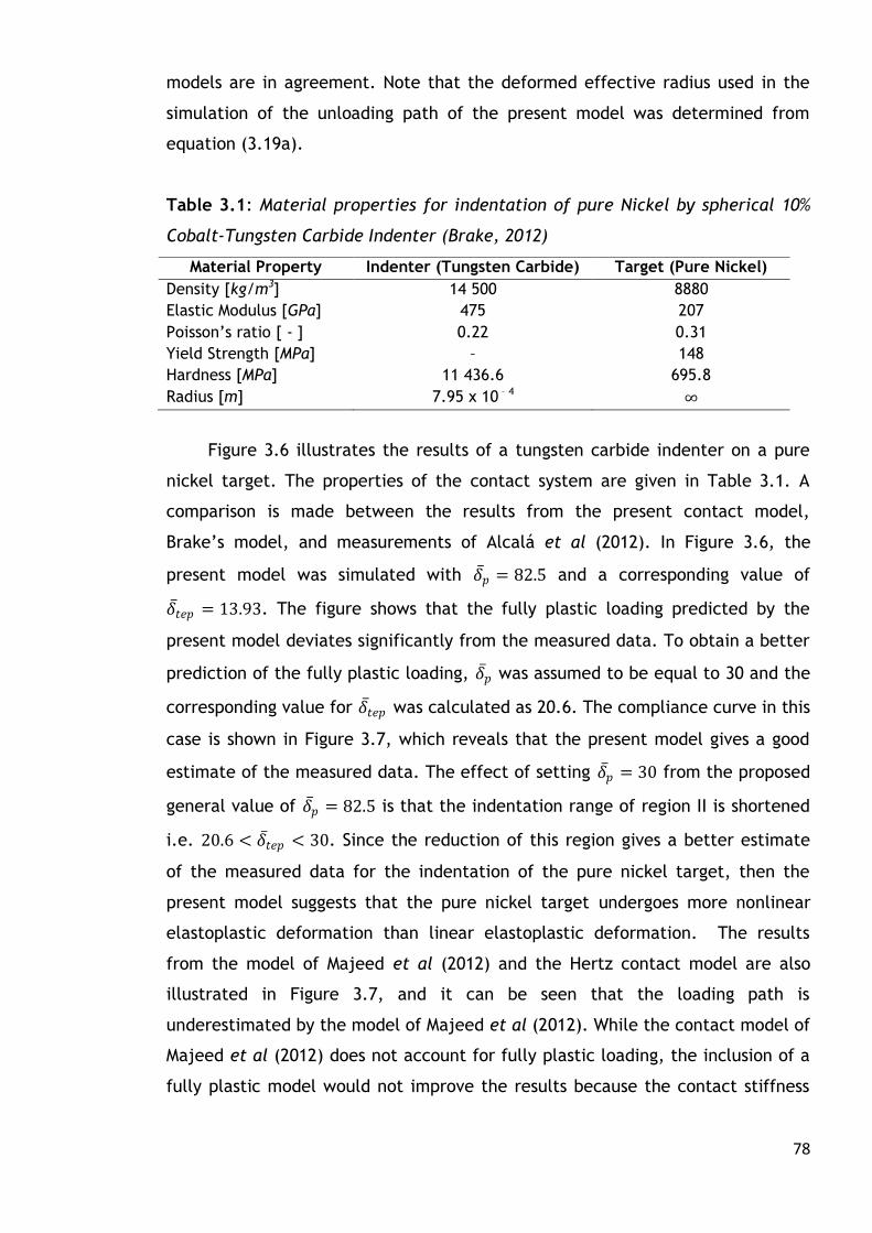
78

models are in agreement. Note that the deformed effective radius used in the

simulation of the unloading path of the present model was determined from

equation (3.19a).

Table 3.1: Material properties for indentation of pure Nickel by spherical 10%

Cobalt-Tungsten Carbide Indenter (Brake, 2012)

Material Property Indenter (Tungsten Carbide) Target (Pure Nickel)

Density [kg/m3] 14 500 8880

Elastic Modulus [GPa] 475 207

Poisson’s ratio [ - ] 0.22 0.31

Yield Strength [MPa] – 148

Hardness [MPa] 11 436.6 695.8

Radius [m] 7.95 x 10 – 4 ∞

Figure 3.6 illustrates the results of a tungsten carbide indenter on a pure

nickel target. The properties of the contact system are given in Table 3.1. A

comparison is made between the results from the present contact model,

Brake’s model, and measurements of Alcalá et al (2012). In Figure 3.6, the

present model was simulated with 𝛿 𝑝 = 82.5 and a corresponding value of

𝛿 𝑡𝑒𝑝 = 13.93. The figure shows that the fully plastic loading predicted by the

present model deviates significantly from the measured data. To obtain a better

prediction of the fully plastic loading, 𝛿 𝑝 was assumed to be equal to 30 and the

corresponding value for 𝛿 𝑡𝑒𝑝 was calculated as 20.6. The compliance curve in this

case is shown in Figure 3.7, which reveals that the present model gives a good

estimate of the measured data. The effect of setting 𝛿 𝑝 = 30 from the proposed

general value of 𝛿 𝑝 = 82.5 is that the indentation range of region II is shortened

i.e. 20.6 < 𝛿 𝑡𝑒𝑝 < 30. Since the reduction of this region gives a better estimate

of the measured data for the indentation of the pure nickel target, then the

present model suggests that the pure nickel target undergoes more nonlinear

elastoplastic deformation than linear elastoplastic deformation. The results

from the model of Majeed et al (2012) and the Hertz contact model are also

illustrated in Figure 3.7, and it can be seen that the loading path is

underestimated by the model of Majeed et al (2012). While the contact model of

Majeed et al (2012) does not account for fully plastic loading, the inclusion of a

fully plastic model would not improve the results because the contact stiffness

79

0

0.2

0.4

0.6

0.8

1

1.2

1.4

1.6

1.8

2

0 0.2 0.4 0.6 0.8 1 1.2

Co

nta

ct f

orc

e (

N)

Indentation (μm)

Present Experiment Brake (2012)

0

0.2

0.4

0.6

0.8

1

1.2

1.4

1.6

1.8

2

0 0.2 0.4 0.6 0.8 1 1.2

Co

nta

ct f

orc

e (

N)

Indentation (μm)

Present Experiment Brake (2012) Majeed et al (2012) Hertz

in the fully plastic loading regime is reduced further compared to the

elastoplastic loading regime, thereby leading to lower contact force estimates.


indentation is well into the fully plastic regime. 𝛿 𝑝 = 82.5; 𝛿 𝑡𝑒𝑝 = 13.93 for the

present model.


indentation is well into the fully plastic regime. 𝛿 𝑝 = 30; 𝛿 𝑡𝑒𝑝 = 20.6 for the

present model.

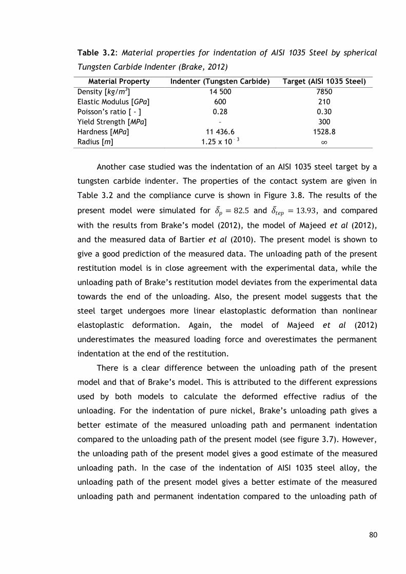
80

Table 3.2: Material properties for indentation of AISI 1035 Steel by spherical

Tungsten Carbide Indenter (Brake, 2012)

Material Property Indenter (Tungsten Carbide) Target (AISI 1035 Steel)

Density [kg/m3] 14 500 7850

Elastic Modulus [GPa] 600 210

Poisson’s ratio [ - ] 0.28 0.30

Yield Strength [MPa] – 300

Hardness [MPa] 11 436.6 1528.8

Radius [m] 1.25 x 10 – 3 ∞

Another case studied was the indentation of an AISI 1035 steel target by a

tungsten carbide indenter. The properties of the contact system are given in

Table 3.2 and the compliance curve is shown in Figure 3.8. The results of the

present model were simulated for 𝛿 𝑝 = 82.5 and 𝛿 𝑡𝑒𝑝 = 13.93, and compared

with the results from Brake’s model (2012), the model of Majeed et al (2012),

and the measured data of Bartier et al (2010). The present model is shown to

give a good prediction of the measured data. The unloading path of the present

restitution model is in close agreement with the experimental data, while the

unloading path of Brake’s restitution model deviates from the experimental data

towards the end of the unloading. Also, the present model suggests that the

steel target undergoes more linear elastoplastic deformation than nonlinear

elastoplastic deformation. Again, the model of Majeed et al (2012)

underestimates the measured loading force and overestimates the permanent

indentation at the end of the restitution.

There is a clear difference between the unloading path of the present

model and that of Brake’s model. This is attributed to the different expressions

used by both models to calculate the deformed effective radius of the

unloading. For the indentation of pure nickel, Brake’s unloading path gives a

better estimate of the measured unloading path and permanent indentation

compared to the unloading path of the present model (see figure 3.7). However,

the unloading path of the present model gives a good estimate of the measured

unloading path. In the case of the indentation of AISI 1035 steel alloy, the

unloading path of the present model gives a better estimate of the measured

unloading path and permanent indentation compared to the unloading path of

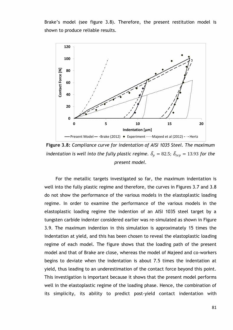
81

0

20

40

60

80

100

120

0 5 10 15 20

Co

nta

ct F

orc

e [

N]

Indentation [μm]

Present Model Brake (2012) Experiment Majeed et al (2012) Hertz

Brake’s model (see figure 3.8). Therefore, the present restitution model is

shown to produce reliable results.

Figure 3.8: Compliance curve for indentation of AISI 1035 Steel. The maximum

indentation is well into the fully plastic regime. 𝛿 𝑝 = 82.5; 𝛿 𝑡𝑒𝑝 = 13.93 for the

present model.

For the metallic targets investigated so far, the maximum indentation is

well into the fully plastic regime and therefore, the curves in Figures 3.7 and 3.8

do not show the performance of the various models in the elastoplastic loading

regime. In order to examine the performance of the various models in the

elastoplastic loading regime the indention of an AISI 1035 steel target by a

tungsten carbide indenter considered earlier was re-simulated as shown in Figure

3.9. The maximum indention in this simulation is approximately 15 times the

indentation at yield, and this has been chosen to reveal the elastoplastic loading

regime of each model. The figure shows that the loading path of the present

model and that of Brake are close, whereas the model of Majeed and co-workers

begins to deviate when the indentation is about 7.5 times the indentation at

yield, thus leading to an underestimation of the contact force beyond this point.

This investigation is important because it shows that the present model performs

well in the elastoplastic regime of the loading phase. Hence, the combination of

its simplicity, its ability to predict post-yield contact indentation with

82

0

0.5

1

1.5

2

2.5

0 0.05 0.1 0.15 0.2 0.25 0.3 0.35 0.4 0.45

Co

nta

ct F

orc

e [

N]

Indentation [μm]

Brake (2012) Present model Majeed et al (2012) Hertz

reasonable accuracy, and the fact that it can be completely evaluated from the

properties of the contact system makes the present contact model an attractive

choice for impact analysis and validation of indentation test results.

Figure 3.9: Comparison of elastoplastic loading regime of present model with

the models of Brake (2012) and Majeed et al (2012) for indentation of AISI 1035

Steel.

3.3.3 Dynamic indentation analysis

During elastoplastic impact of a half-space by a spherical impactor part of

the initial kinetic energy of the impactor is dissipated as plastic deformation

and/or damage of the target. Consequently, the final rebound velocity of the

impactor is less than the initial impact velocity. The severity of the impact and

the impact energy absorption capacity of the target are measured by the

coefficient of restitution. It has been shown that the coefficient of restitution is

dependent on velocity (Johnson, 1985; Goldsmith, 2001; Jackson et al, 2009).

Hence, measurements of the coefficient of restitution over a velocity range can

be used to validate contact models. In this section, an analytical approach is

formulated for determining the coefficient of restitution and applied to the new

contact model formulated in Section 3.2. The coefficient of restitution results

derived by the application of the analytical approach to the new contact model

was compared with published measurements of the coefficient of restitution in

order to validate the new contact model.

83

3.3.3.1 Analytical method for determination of coefficient of

restitution

Stronge (2000a) gave three definitions of the coefficient of restitution

namely: the kinematic, kinetic and energetic coefficient of restitution. The

kinematic coefficient of restitution is the negative of the ratio of the final

velocity of restitution to the initial impact velocity. The ratio of the impulse

change during restitution to the impulse change during impact loading is known

as the kinetic coefficient of restitution. The square of the energetic coefficient

of restitution is equal to the negative of the ratio of the elastic energy released

during restitution to the energy absorbed during impact loading. It was shown by

Stronge (2000a) that these three definitions of the coefficient of restitution are

equivalent unless the impacting bodies are rough, the configuration is eccentric

and the direction of slip varies during collision. For the normal impact of a rigid

spherical mass on a compliant flat half-space, as considered here, the three

definitions are equivalent.

Stronge (2000a) applied the energetic approach to derive analytical

expressions for calculating the coefficient of restitution. Here the kinematic

approach has been applied to determine the coefficient of restitution using the

new contact model to estimate the impact force. An analytical approach was

developed to determine the final rebound velocity for an elastoplastic half-space

impact. The approach combines closed-form integrals of the equations of motion

for the loading and unloading regimes and a simple algorithm for calculating the

maximum indentation and force of an elastoplastic impact.

Approximate analytical solutions have been derived for the fraction of

impact energy dissipated as a non-recoverable elastic wave during elastic impact

(Hunter, 1957) and elastic-plastic impact (Hutchings, 1979) on a half-space, but

the fraction is negligible in both cases (Hunter, 1957; Hutchings, 1979).

Furthermore, Johnson (1985) has shown that the elastoplastic impact response

of a metallic half-space can be accurately determined by assuming quasi-static

loading and unloading for impact velocities up to 500 [m/s]. Therefore, the

impact force for such rate-independent impact events can be determined from

an appropriate contact model.

The equation of motion for the impact of a half-space target by a rigid

spherical impactor is given as:

84

𝑚𝑖𝛿 + 𝐹 = 0 (3.53)

where 𝑚𝑖 is the mass of the impactor; 𝛿 is the indentation of the target, which is

equal to the displacement of the impactor, and the initial conditions are

𝛿 0 = 0, 𝛿 0 = 𝑉0; 𝑉0 is the initial impact velocity, 𝐹 is the impact force and it

is subject to the restriction in equation (3.54).

𝐹 = 𝐹 𝛿 𝑖𝑓 𝐹 > 0 0 𝑖𝑓 𝐹 ≤ 0

(3.54)

Equation (3.53) can be rewritten as

𝑚𝑖𝛿 𝑑𝛿 𝑡

𝑡0

= − 𝐹(𝛿)𝑑𝛿𝑡

𝑡0

(3.55)

where 𝑡0 is the time at the onset of an impact loading or unloading regime.

Substituting equations (3.26) to (3.30) in (3.55) and evaluating the resulting

integral, the following equations were derived for calculating the velocity in the

loading and unloading regimes.

Loading regimes

𝛿 = 𝑉02 −

4𝐾𝑕5𝑚𝑖

𝛿5/2 1/2

0 ≤ 𝛿 ≤ 𝛿𝑦 (3.56)

𝛿 = 𝑉𝑦2 −

4𝐾𝑕5𝑚𝑖

𝛿 − 𝛿𝑦 5/2

−2𝐾𝑕𝑚𝑖

𝛿𝑦3/2 𝛿 − 𝛿𝑦

1/2

𝛿𝑦 ≤ 𝛿 ≤ 𝛿𝑡𝑒𝑝 (3.57)

𝛿 = 𝑉𝑡𝑒𝑝2 −

𝐾𝑙𝑚𝑖

𝛿 − 𝛿𝑡𝑒𝑝 2−

95𝐾𝑕𝑚𝑖

𝛿𝑦3/2 𝛿 − 𝛿𝑡𝑒𝑝

1/2

𝛿𝑡𝑒𝑝 ≤ 𝛿 ≤ 𝛿𝑝 (3.58)

𝛿 = 𝑉𝑝2 −

𝐾𝑝

𝑚𝑖 𝛿 − 𝛿𝑝

2−

2𝐹𝑝

𝑚𝑖 𝛿 − 𝛿𝑝

1/2

𝛿𝑝 ≤ 𝛿 ≤ 𝛿𝑚 (3.59)

Unloading regime

𝛿 = − 4𝐾𝑢5𝑚𝑖

𝛿𝑚 − 𝛿𝑓 5/2

− 𝛿 − 𝛿𝑓 5/2

1/2

𝛿𝑓 ≤ 𝛿 ≤ 𝛿𝑚 (3.60)

In deriving equation (3.58) 𝛿𝑡𝑒𝑝 = 13.93𝛿𝑦 was applied to simplify the resulting

expression. The velocities at the transition from one loading regime to the other

can be determined from equations (3.56) to (3.58) as follows.

𝑉𝑦 = 𝑉02 −

4𝐾𝑕5𝑚𝑖

𝛿𝑦5/2

1/2

(3.61)

𝑉𝑡𝑒𝑝 = 𝑉𝑦2 −

4𝐾𝑕5𝑚𝑖

𝛿𝑡𝑒𝑝 − 𝛿𝑦 5/2

−2𝐾𝑕𝑚𝑖

𝛿𝑦3/2 𝛿𝑡𝑒𝑝 − 𝛿𝑦

1/2

(3.62)

𝑉𝑝 = 𝑉𝑡𝑒𝑝2 −

𝐾𝑙𝑚𝑖

𝛿𝑝 − 𝛿𝑡𝑒𝑝 2−

95𝐾𝑕𝑚𝑖

𝛿𝑦3/2 𝛿𝑝 − 𝛿𝑡𝑒𝑝

1/2

(3.63)

85

If 𝛿𝑝 = 82.5𝛿𝑦 and the corresponding indentation 𝛿𝑡𝑒𝑝 = 13.93𝛿𝑦 are substituted

in equations (3.62) and (3.63), then

𝑉𝑡𝑒𝑝 = 𝑉𝑦2 − 506.795

𝐾𝑕𝑚𝑖

𝛿𝑦5/2

1/2

(3.64)

𝑉𝑝 = 𝑉𝑡𝑒𝑝2 − 31904.112

𝐾𝑕𝑚𝑖

𝛿𝑦5/2

1/2

(3.65)

To complete the analytical method for calculating the coefficient of

restitution the maximum indentation and impact force must be known. The

relative velocity of the impactor and target during half-space impact is zero at

the maximum indentation. This condition can be used to determine the

maximum indentation and impact force of a half-space impact by using energy

balance principles. However, for impacts on slender (flexible) targets, this

condition can occur more than once during the impact thus resulting in more

than one extremum. Furthermore, the interactions between vibrations of the

target and the indentation introduce complications which make the energy

balance approach impractical for impact on slender targets (Abrate, 1998).

During an elastoplastic impact on a half-space, the impact energy of the

impactor is dissipated through various mechanisms such as elastic compression,

elastic waves, plastic deformation, heat and sound. Johnson (1985) showed that

for impact velocities up to 500 [m/s], all other mechanisms of impact energy

dissipation can be neglected except for elastic compression and plastic

deformation. The elastic compression energy is restored back to the impactor

during unloading and the plastic deformation is dissipated in the half-space

target as a permanent indentation. The range of impact velocities up to 500

[m/s] covers low to medium velocity impacts where strain rate effects can be

neglected, and therefore, the impact event can be modelled using quasi-static

assumptions (Johnson, 1985). For such impact events, the energy balance

approach can be applied with the following assumptions: (i) no energy is lost

from the impact system and (ii) the initial kinetic energy of the impactor is

equal to the deformation work on the target i.e. elastic and plastic deformation.

Based on the energy balance approach, the following expression holds:

1

2𝑚𝑖𝑉0 = 𝐹

𝛿𝑚

0

𝑑𝛿 (3.66)

where 𝐹 represents a general impact force that can be in any of the loading

regimes.

86

In a typical impact event, a spherical impactor with known mass and

velocity impacting a half-space target produces a definite maximum indentation

that falls into one of the loading regimes discussed above. Therefore, it is

necessary to determine the loading regime in which the maximum indentation is

located, so that the appropriate force-indentation relationship(s) can be used in

the impact analysis. Since the contact force can be represented as a piecewise

continuous function of indentation, an iterative algorithm based on the energy

balance is proposed here to determine the maximum indentation and impact

force. In view of the fact that the impact loading starts from the elastic regime,

the first step is to compare the total deformation work done up to the end of

the elastic regime 𝑊𝑦 to the kinetic energy 𝐾𝐸 of the impactor. If 𝐾𝐸 < 𝑊𝑦 ,

then the maximum indentation is in the elastic regime, otherwise the total

deformation work done up the end of region I 𝑊𝑡𝑒𝑝 is determined and

compared with the 𝐾𝐸. Again, if 𝐾𝐸 < 𝑊𝑡𝑒𝑝 , then the maximum indentation is in

region I, otherwise the process is repeated until the maximum indentation is

located in one of the loading regimes. The algorithm for this procedure is shown

as a flowchart in Figure 3.10. Also, the total deformation work done from the

beginning of the loading to each of the transition points in the loading regime

are derived in appendix A.2.

To demonstrate the validity of this approach, the impact of a tungsten

carbide ball on a mild steel half-space was investigated. The properties of the

steel material are: Young’s modulus = 210 [GPa], Poisson’s ratio = 0.30 [-], and

yield strength = 1000 [MPa]; and the properties of the tungsten carbide ball are:

density = 14500 [kg/m3], Young’s modulus = 600 [GPa], and Poisson’s ratio =

0.28. The diameter of the ball is 20 [mm] and the initial impact velocity is 5

[m/s]. The mass and initial KE of impactor was calculated as 0.06074 [kg] and

0.759 [J] respectively. Using the flowchart in Figure 3.10, the maximum

indentation for this impact event was located in the linear elastoplastic loading

regime and calculated as 101.623 [µm]. Hence, equations (3.56) to (3.58) were

used to simulate the velocity-indentation response for the loading and equation

(3.60) was used to simulate the velocity-indentation response for the unloading.

The results obtained are plotted in Figure 3.11. The figure also shows results

obtained by direct numerical integration of equation (3.53) with equations (3.26

87

– 3.30) used to estimate the impact force. The results of the numerical

integration are in excellent agreement with the analytical method.

Figure 3.10: Method to determine the maximum indentation and force during

impact.

STOP

START

Is 𝐾𝐸 < 𝑊𝑦?

Calculate all the constants for the loading regimes

Then 0 < 𝛿𝑚 < 𝛿𝑦 . Replace

𝛿𝑦 by 𝛿𝑚 in 𝑊𝑦 and equate

the result to 𝐾𝐸

Yes

Yes

Yes

No

No

No

Calculate 𝐾𝐸 = 0.5𝑚𝑖𝑉02

Calculate the total work done up to the end of the elastic regime, 𝑊𝑦

Calculate the total work done up to the end of the region I, 𝑊𝑡𝑒𝑝

Is 𝐾𝐸 < 𝑊𝑡𝑒𝑝 ?

Calculate the total work done up to the end of the region II, 𝑊𝑝

Is 𝐾𝐸 < 𝑊𝑝?

Then 𝛿𝑚 > 𝛿𝑝 . Equate 𝐾𝐸 to

the sum of 𝑊𝑝 and 𝑊𝑓𝑝

Then 𝛿𝑦 < 𝛿𝑚 < 𝛿𝑡𝑒𝑝 .

Replace 𝛿𝑡𝑒𝑝 by 𝛿𝑚 in 𝑊𝑡𝑒𝑝

and equate the result to 𝐾𝐸

Then 𝛿𝑡𝑒𝑝 < 𝛿𝑚 < 𝛿𝑝 .

Replace 𝛿𝑝 by 𝛿𝑚 in 𝑊𝑝 and

equate the result to 𝐾𝐸

Solve the equation to find 𝛿𝑚 , and

then solve for 𝐹𝑚 using the formula

of the regime in which 𝛿𝑚 lies.

88

-5

-4

-3

-2

-1

0

1

2

3

4

5

6

0 0.02 0.04 0.06 0.08 0.1 0.12Ve

loci

ty [m

/s]

Indentation [mm]

Analytical

Numerical

Figure 3.11: Validation of analytical method for calculating the impactor

velocity profile during half-space impact.

3.3.3.2 Validation of new contact model using dynamic indentation

measurements

The most commonly used definition of coefficient of restitution is the

kinematic definition and it is expressed mathematically as:

𝑒 = − 𝑉𝑓

𝑉0 (3.67)

where 𝑉𝑓 is the rebound velocity of the impactor at the end of the restitution. In

Section 3.3.3.1 an analytical method was developed that can be used to

determine the velocity-indentation profile for the loading and restitution stages

of an elastoplastic impact, and the method was demonstrated using the new

contact model presented in Section 3.2. At the end of the restitution 𝛿 = 𝛿𝑓, and

using equation (3.60)

𝑉𝑓 = − 4𝐾𝑢5𝑚𝑖

𝛿𝑚 − 𝛿𝑓 5/2

1/2

(3.68)

𝑉𝑓 depends on the maximum indentation and impact force. The energy-balance

algorithm developed earlier can be used to determine the maximum indentation

and impact force. The values of the maximum indentation and impact force so

obtained are substituted into equation (3.68) to calculate 𝑉𝑓, which is then used

to calculate the coefficient of restitution.

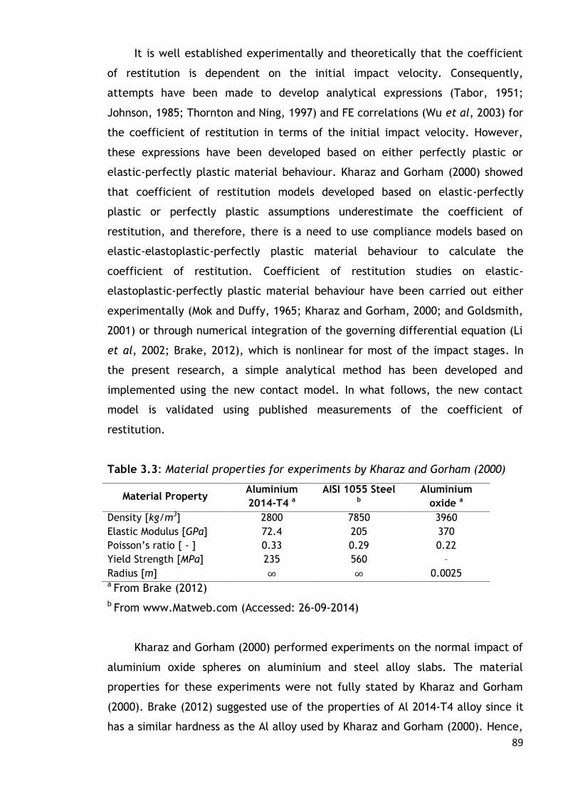
89

It is well established experimentally and theoretically that the coefficient

of restitution is dependent on the initial impact velocity. Consequently,

attempts have been made to develop analytical expressions (Tabor, 1951;

Johnson, 1985; Thornton and Ning, 1997) and FE correlations (Wu et al, 2003) for

the coefficient of restitution in terms of the initial impact velocity. However,

these expressions have been developed based on either perfectly plastic or

elastic-perfectly plastic material behaviour. Kharaz and Gorham (2000) showed

that coefficient of restitution models developed based on elastic-perfectly

plastic or perfectly plastic assumptions underestimate the coefficient of

restitution, and therefore, there is a need to use compliance models based on

elastic-elastoplastic-perfectly plastic material behaviour to calculate the

coefficient of restitution. Coefficient of restitution studies on elastic-

elastoplastic-perfectly plastic material behaviour have been carried out either

experimentally (Mok and Duffy, 1965; Kharaz and Gorham, 2000; and Goldsmith,

2001) or through numerical integration of the governing differential equation (Li

et al, 2002; Brake, 2012), which is nonlinear for most of the impact stages. In

the present research, a simple analytical method has been developed and

implemented using the new contact model. In what follows, the new contact

model is validated using published measurements of the coefficient of

restitution.

Table 3.3: Material properties for experiments by Kharaz and Gorham (2000)

Material Property Aluminium

2014-T4 a

AISI 1055 Steel

b

Aluminium

oxide a

Density [kg/m3] 2800 7850 3960

Elastic Modulus [GPa] 72.4 205 370

Poisson’s ratio [ - ] 0.33 0.29 0.22

Yield Strength [MPa] 235 560 –

Radius [m] ∞ ∞ 0.0025 a From Brake (2012)

b From www.Matweb.com (Accessed: 26-09-2014)

Kharaz and Gorham (2000) performed experiments on the normal impact of

aluminium oxide spheres on aluminium and steel alloy slabs. The material

properties for these experiments were not fully stated by Kharaz and Gorham

(2000). Brake (2012) suggested use of the properties of Al 2014-T4 alloy since it

has a similar hardness as the Al alloy used by Kharaz and Gorham (2000). Hence,

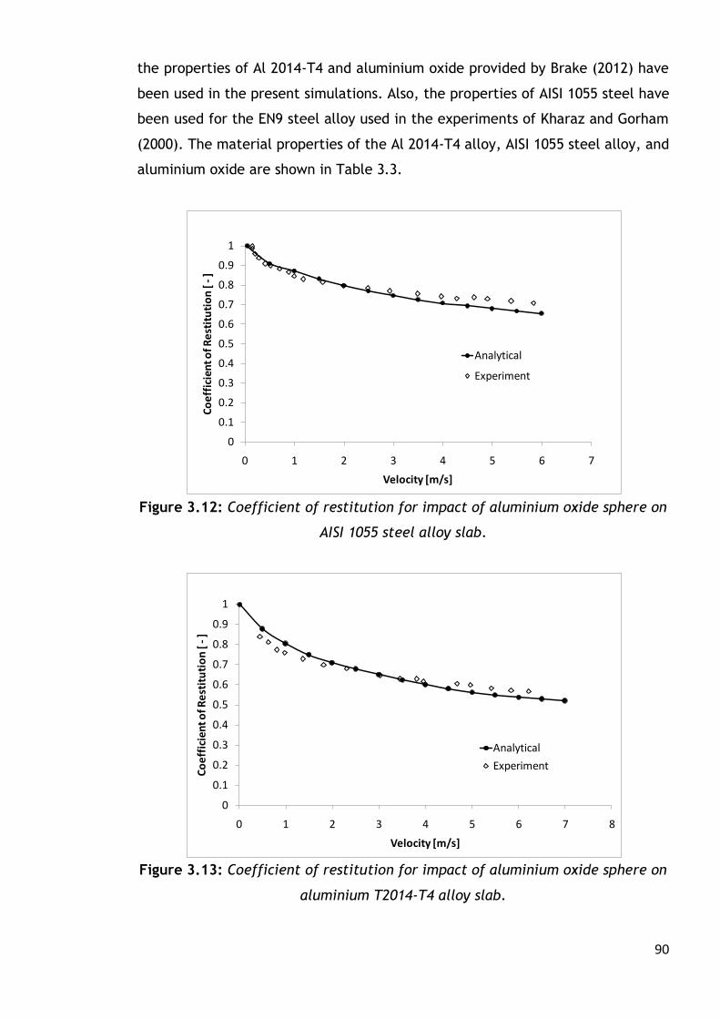
90

0

0.1

0.2

0.3

0.4

0.5

0.6

0.7

0.8

0.9

1

0 1 2 3 4 5 6 7 8

Co

eff

icie

nt o

f Re

stit

uti

on

[ -]

Velocity [m/s]

Analytical

Experiment

0

0.1

0.2

0.3

0.4

0.5

0.6

0.7

0.8

0.9

1

0 1 2 3 4 5 6 7

Co

eff

icie

nt o

f Re

stit

uti

on

[ -]

Velocity [m/s]

Analytical

Experiment

the properties of Al 2014-T4 and aluminium oxide provided by Brake (2012) have

been used in the present simulations. Also, the properties of AISI 1055 steel have

been used for the EN9 steel alloy used in the experiments of Kharaz and Gorham

(2000). The material properties of the Al 2014-T4 alloy, AISI 1055 steel alloy, and

aluminium oxide are shown in Table 3.3.


AISI 1055 steel alloy slab.


aluminium T2014-T4 alloy slab.

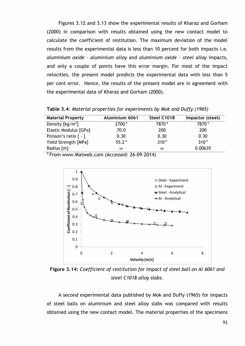
91

0

0.1

0.2

0.3

0.4

0.5

0.6

0.7

0.8

0.9

1

0 2 4 6 8

Co

eff

icie

nt o

f Re

stit

uti

on

[ -]

Velocity [m/s]

Steel - Experiment

Al - Experiment

Steel - Analytical

Al - Analytical

Figures 3.12 and 3.13 show the experimental results of Kharaz and Gorham

(2000) in comparison with results obtained using the new contact model to

calculate the coefficient of restitution. The maximum deviation of the model

results from the experimental data is less than 10 percent for both impacts i.e.

aluminium oxide – aluminium alloy and aluminium oxide – steel alloy impacts,

and only a couple of points have this error margin. For most of the impact

velocities, the present model predicts the experimental data with less than 5

per cent error. Hence, the results of the present model are in agreement with

the experimental data of Kharaz and Gorham (2000).

Table 3.4: Material properties for experiments by Mok and Duffy (1965)

Material Property Aluminium 6061 Steel C1018 Impactor (steel)

Density [kg/m3] 2700 a 7870 a 7870 a

Elastic Modulus [GPa] 70.0 200 200

Poisson’s ratio [ - ] 0.30 0.30 0.30

Yield Strength [MPa] 55.2 a 310 a 310 a

Radius [m] ∞ ∞ 0.00635 a From www.Matweb.com (Accessed: 26-09-2014)

Figure 3.14: Coefficient of restitution for impact of steel ball on Al 6061 and

steel C1018 alloy slabs.

A second experimental data published by Mok and Duffy (1965) for impacts

of steel balls on aluminium and steel alloy slabs was compared with results

obtained using the new contact model. The material properties of the specimens

92

used in the experiments are shown in Table 3.4. The results obtained using the

new contact model and the experimental measurements of Mok and Duffy (1965)

are shown in Figure 3.14. The figure reveals that the model results are in good

agreement with the experimental measurements of Mok and Duffy (1965).


Analytical models for contact indentation of elastic-elastoplastic-fully

plastic materials are relatively few despite the fact that many engineering

materials fall under this category. The published contact models for the

indentation of elastic-elastoplastic-fully plastic materials are either finite

element correlations that are case specific or quite complex analytical models.

In this chapter, some of the previously published analytical contact models for

indentation of elastic-elastoplastic-fully plastic materials were reviewed and

discussed. A simple contact model that accounts for post-yield effects in the

loading and restitution stages of the indentation of an elastic-elastoplastic-fully

plastic material by a spherical indenter was formulated. In line with observations

from previous experiments and FE results reported in the literature (Majeed et

al, 2012), the elastoplastic loading regime was divided into two regions,

nonlinear and linear, and modelled accordingly. Simple expressions have been

derived for all constants in the present contact model and the constants can be

completely evaluated from the geometric and material properties of the contact

system. Also, the model for the restitution phase allows for unloading from any

of the loading regimes. Results obtained from the simulation of the new contact

model were compared with published static and dynamic indentation

experiments, and the new contact model was found to give a good prediction of

the experimental data. A key advantage of the new contact model is that it can

be readily used for impact modelling and allows for computational tractability

because all the stages for the loading and unloading are expressed in the form of

Meyer’s law (Big-Alabo et al, 2014a). The contact modelling approach used here

is supported by the observation of Kharaz and Gorham (2000) that compliance

models in the form of Meyer’s law can be used to model the elastoplastic

indentation of elastic-elastoplastic-fully plastic materials.

A simple algorithm for calculating the maximum indentation and contact

force during half-space impact has been proposed in this study. The approach

93

applies energy balance principles and it is applicable to impact events that can

be modelled using quasi-static assumptions i.e. low to medium velocity impacts.

An analytical method for calculating the coefficient of restitution during

half-space impact was also presented. The method uses the closed-form integral

of the governing equation for the restitution of a half-space impact and the

maximum indentation and contact force values obtained from the energy

balance algorithm to determine the rebound velocity. The value of the rebound

velocity so obtained is used to calculate the coefficient of restitution from

equation (3.67). The analytical method for calculating the coefficient of

restitution can be applied to other contact models (Johnson, 1985; Stronge

2000a; Brake, 2012) for post-yield indentation of elastic-elastoplastic-perfectly

plastic materials. The approach is simple and can be used to avoid the possible

issues of solution convergence associated with numerical integration of the

governing nonlinear equation of a half-space impact.

94

CHAPTER FOUR

IMPACT ANALYSIS OF RECTANGULAR PLATES SUBJECTED TO NORMAL IMPACT OF A RIGID SPHERICAL

IMPACTOR

Chapter summary

This chapter presents analytical investigations on the normal (direction

perpendicular to the plane of the plate) impact response of rectangular plates

impacted by a rigid mass with spherical contact surface. The focus of this

chapter is on: (a) the formulation of analytical models for the elastoplastic

impact response of transversely inflexible (very thick) and transversely flexible

(thin to moderately thick) rectangular plates, (b) the solution to these models

that are generally in the form of nonlinear differential equations, and (c) the

effect of different impact parameters on the elastoplastic impact response of

transversely flexible rectangular plates. First, a review is presented of analytical

modelling approaches for the normal impact of rigid blunt objects on compliant

targets. Next, the elastoplastic impact response of transversely inflexible and

flexible rectangular plates is investigated using the new contact model,

previously presented in chapter 3, and also using other existing static contact

models found in the literature to estimate the impact force. Additionally, the

formulation and implementation of a new analytical solution algorithm for the

solution of nonlinear impact models of transversely inflexible plates is

presented. The implications for applying the solution algorithm to determine the

impact response of transversely flexible plates are also discussed.

4.1 Review of analytical models for rigid object impact

on compliant targets

According to Goldsmith (2001), the first attempt at formulating analytical

models for the impact dynamics of a rigid blunt object striking a flexible

structure, incorporating the interactions between the local and global

deformation of the impact system, can be attributed to Sears (1908) and

Timoshenko (1913). The elastic impact of a beam struck axially (Sears, 1908)

and transversely (Timoshenko, 1913) by a spherical steel ball was modelled using

95

the Hertz contact theory and the beam deformation theory. This concept of

combining local contact mechanics and structural mechanics in modelling rigid

blunt object impact has since been extended to plates and shells. Several impact

modelling approaches have been applied based on the response characteristics

of the impact system, and these have been summarised in various papers

(Abrate, 1998; 2001; 2011; and Chai and Zhu, 2011). Hence, the selection of an

appropriate modelling approach for a given impact event is important if

accurate results are to be obtained.

To determine the right impact modelling approach for a particular impact

event, a means of classifying the impact response must first be established.

There are different types of impact response classification reported in the

literature. One early classification is based on the impact velocity, and it is used

to classify impact events as low-, medium-, and high-velocity impact (Chai and

Zhu, 2011). For a low-velocity impact, there is no visible damage although

localised internal damage may occur, whereas there is visible and easily

detectable large damage during high-velocity impact that may sometimes

include perforation and tear. For medium-velocity impact, there may be a small

visible level of damage but internal damage is likely to be considerably larger.

Another classification is based on impact duration. According to this

classification, the following impact responses are identified (Olsson, 2000; Chai

and Zhu, 2011):

(i) When the ratio of the impact duration to the time taken for the first stress

wave to propagate through the thickness of the structure is less than or

approximately equal to one, the impact response is dominated by 3-D wave

propagation. This type of impact response is normally associated with

ballistic impacts, which causes visible damage and sometimes perforation of

the target.

(ii) When the ratio of the impact duration to the time taken for vibration waves

to reach the boundary is equal to, or just greater than one, the impact

response is dominated by shear and flexural waves and is a dynamic event.

Typical cases involve impact on flexible aero-structures due to hailstone and

runway debris.

(iii) When the ratio of the impact duration to the time taken for vibration waves

to reach the boundary is far greater than one, the impact response is

dominated by the lowest mode of vibration. The response can be modelled

96

using quasi-static analysis, and a typical case is drop-weight impact normally

used in experimental investigations.

Olsson (2000) argued that the limits of the impact velocity criterion is not

clearly defined, and suggested the use of a mass ratio instead i.e.

impactor/plate mass ratio (𝜇𝑚 ). Based on Olsson’s mass criterion, the impact

can be divided into small, intermediate and large mass impact. For small mass

impact 𝜇𝑚 < 1/5, for large mass impact 𝜇𝑚 > 2, and for intermediate mass

impact the mass ratio lies in the range 1/5 < 𝜇𝑚 < 2. The response is wave-

controlled for small mass impacts and can be modelled using the closed-form

solution in Olsson (1992). For large mass impacts, the response is fully boundary-

controlled and can be modelled based on quasi-static assumptions using the

energy model (Abrate, 1998; Chai and Zhu, 2011) and/or spring-mass model

(Chai and Zhu, 2011). For intermediate mass impacts, the response is dominated

by highly dynamic interactions between flexural waves, shear waves and local

indentation. A model that accounts for all these effects is required for accurate

analysis. The mass criterion of Olsson is limited to impact responses in which the

impact duration is much longer than the transition time for the through-the-

thickness waves, i.e. class (ii) and (iii) in the impact duration classification

system described above.

Christoforou and Yigit (1995) used a normalisation technique to investigate

the parameters that influence the impact response of a beam based on an

elastic-plastic contact law. By normalising the differential equations governing

the transverse impact of the beam, all the parameters influencing the impact

response were identified. Four non-dimensional parameters that influence the

impact response of the beam were obtained, of which the impactor-beam mass

ratio was one. The study showed that the mass ratio is not the only parameter

influencing the system’s impact response and when considered alone, it is not

sufficient information for characterisation of impact events. Christoforou and

Yigit (1995) concluded that the normalisation technique can be used to obtain

the parameters that influence an impact event and these parameters can be

used for scaling purposes.

Yigit and Christoforou (1995) used the normalisation technique to

determine the parameters that influence the impact response of a beam based

on the linearised version of an elastic-plastic contact law. Three non-

dimensional parameters that influence the impact response of the beam were

97

identified in that study. The parameters were regrouped into a single non-

dimensional parameter called the dynamic impact number (DIN). The latter was

used to classify the impact response as locally dominated, quasi-static, or

dynamic. The DIN was found to vary from zero to one. A value of zero represents

a locally-dominated response – the so called half-space impact – while a value of

one represents a quasi-static response. When the DIN is between 0 and 1, the

response is classified as dynamic. Also, a dynamic ratio was defined as the ratio

of the maximum impact force obtained from the dynamic solution to the

maximum impact force obtained from an equivalent half-space solution, and this

dynamic ratio was found to be a dependent on the DIN.

Christoforou and Yigit (1998a) used the normalisation technique to

investigate the impact response of a plate based on a linearised elastic-plastic

contact law. The analysis showed that the impact response of the plate was

governed by two non-dimensional parameters related to the dynamic ratio; the

relative stiffness (𝜆), which accounts for the mechanical stiffness effect, and the

loss factor (휁), which accounts for the material damping effect. A

characterisation diagram was developed which showed that the relationship

between the dynamic ratio and the loss factor can be used to characterise the

response of the plate for different plate stiffnesses. The characterisation

diagram was used to classify the impact response of the plate as local,

transitional (dynamic), and fully global (quasi-static). The relative stiffness was

found to govern the quasi-static response while the loss factor governed the

infinite plate (wave-controlled or initial) response. The local response was

shown to be governed by an additional parameter; a non-dimensional velocity

called the ‘characteristic impact parameter’. The characteristic impact

parameter was normalised to unity in this analysis. The transitional response was

governed by all three parameters i.e. relative stiffness, the loss factor and

characteristic impact parameter. However, the characterisation diagram was

obtained based on a linearised elastic-plastic contact law, an approximation of

actual contact behaviour, which does not account for certain details of the

impact response (e.g. permanent indentation) and is capable of introducing

significant errors in the estimation of the impact response history (Yigit and

Christoforou, 1995).

In conclusion, there is no universal impact response classification

parameter or approach. Although the classification approaches based on a single

98

variable such as impact velocity, time, mass, and energy have proven to be

useful, a combination of factors obtained using the normalisation technique

shows more potential and can provide a wider scope of application.

Nevertheless, all the classification techniques considered here are important and

knowledge of the various techniques is necessary when deciding the impact

modelling approach to be used for a particular impact event. The characteristics

and solution methods for the impact response of plates, based on the different

classification methods described in the above review, are summarised in Figure

4.1. Chia and Zhu (2011) presented a similar classification diagram but the one

presented in Figure 4.1 is more detailed. The decision boxes in Figure 4.1 are

used to select the classification method. For example, the first decision box

raises the question: Is the classification based on impact velocity?

Moving now to modelling approaches, Abrate (1998, 2001) presented an

overview of various impact models and grouped these models into four

categories namely: (a) spring-mass models, (b) energy-balance models, (c)

complete models, and (d) infinite plate models. These models are now briefly

explained, and their applications and limitations are discussed.

99

Figure 4.1: Characteristics and solution methods for different impact classifications.

100

(a) (b) Mi

xi Kc

xi

Mi

Kc

Mp

Km

Ks

Kb xp

Mp

Km

Ks

Kb xp

(c)

4.1.1 The spring-mass model

According to this model, the impactor and plate are represented by

equivalent rigid masses while the plate and contact stiffnesses are represented

by equivalent springs. In the complete two-degree of freedom (DOF) model,

there are two nonlinear springs (for the contact and membrane stiffnesses) and

two linear springs (for the bending and shear stiffnesses) – see Figure 4.2a. The

single-DOF spring-mass model is normally used for a case where the local

indentation is negligible i.e. quasi-static bending response (Figure 4.2b) or the

vibration response of the plate is negligible i.e. half-space impact response

(Figure 4.2c). Anderson (2005) used a single-DOF model to study the response of

composite sandwich laminates to large mass impact. Olsson (2002) studied the

response of a composite sandwich plate to a small mass impact using a single-

DOF spring-mass model with a dashpot. Half-space impact analysis using a single-

DOF model has been discussed by Abrate (1998, 2001), and can be used to

validate the dynamic indentation test results (Brake, 2012). Most studies that

use the 2-DOF spring-mass system to model the impact response of a plate

ignore the membrane stiffness i.e. 𝐾𝑚 = 0 (Abrate, 1998), and in some studies

the contact stiffness is linearised (Khalili et al, 2007a; 2007b).

Figure 4.2: Spring-mass models (a) Complete 2-DOF (b) SDOF for quasi-static

impact (c) SDOF for half-space impact.

Equations for spring-mass models

𝑚𝑝𝑥 𝑝 + 𝐾𝑏𝑠𝑥𝑝 + 𝐾𝑚𝑥𝑝3 − 𝐹 = 0 (4.1)

𝑚𝑖𝑥 𝑖 + 𝐹 = 0 (4.2)

𝐹 = 𝐾𝑐𝛿𝑞 (4.3)

101

where 𝛿 = 𝑥𝑖 − 𝑥𝑝 is the indentation, 𝑞 is the contact law power exponent which

is equal to 3/2 for Hertzian contact, and 1/𝐾𝑏𝑠 = 1/𝐾𝑏 + 1/𝐾𝑠. The subscripts 𝑖

and 𝑝 represent the impactor and plate respectively. The formulas for the

stiffnesses (𝐾𝑏 ,𝐾𝑠 ,𝐾𝑚 ) can be found in Olsson (2001) and Chai and Zhu (2011).

Equations (4.1 – 4.3) are the complete set of equations for the 2-DOF spring-

mass system (Figure 4.2a). For Figure 4.2b, equations (4.1) and (4.3) are used

with the assumption that 𝑥 𝑝 ≅ 0 for quasi-static analysis. For Figure 4.2c,

equations (4.2) and (4.3) are used with the assumption that 𝑥𝑝 ≅ 0 for half-space

analysis.

4.1.2 The energy-balance model

The energy-balance model is normally based on the assumption that both

the local deformation and bending of the plate occur quasi-statically. Therefore,

at the maximum indentation the velocity of the impactor is zero and the initial

kinetic energy of the impactor is completely transferred to the plate without any

loss. The initial kinetic energy of the impactor is converted into the following

energy components in the structure: bending, shear, membrane, contact and

damage energies (Abrate, 1998). Mathematically, we can write:

1

2𝑚𝑖𝑉0

2 = 𝐸𝑏 + 𝐸𝑠 + 𝐸𝑚 + 𝐸𝑐 + 𝐸𝑑 (4.4)

A valid assumption for quasi-static bending of a plate is that its inertia can be

neglected. Hence, from equation (4.1):

𝐹 = 𝐾𝑏𝑠𝑥 𝑝 + 𝐾𝑚𝑥 𝑝3 (4.5)

where 𝑥 𝑝 is the maximum displacement of the plate at the impact point. Some

impact analyses are carried out up to damage initiation so that 𝐸𝑑 is usually

neglected when using equation (4.4) (Abrate, 1998). The contact force obtained

by neglecting 𝐸𝑑 can be used to determine the onset and propagation of

delamination damage (Olsson, 2001; 2002). Using equations (4.3 – 4.5), applying

the Hertz contact model, and assuming that 𝐸𝑑 = 0 it can be shown that (Abrate,

1998; Olsson, 2002):

1

2𝑚𝑖𝑉0

2 =1

2𝐾𝑏𝑠𝑥 𝑝

2 +1

4𝐾𝑚𝑥 𝑝

4 +2

5𝐾𝑐−2

3 𝐾𝑏𝑠𝑥 𝑝 + 𝐾𝑚𝑥 𝑝3

53 (4.6)

Equation (4.6) can be solved numerically to obtain the maximum displacement

of the plate, from which the maximum contact force and indentation can be

obtained using equations (4.5) and (4.3) respectively. The energy-balance model

102

is used where the contact force history is unimportant and the impact response

of the plate is not significantly affected by the contact law. Foo et al (2011)

used the energy-balance approach to predict the low-velocity impact response

of a sandwich composite plate, while Olsson (2002) used the energy-balance

approach to predict the impact response and damage in sandwich panels.

4.1.3 The infinite plate model

The infinite plate model was originally formulated by Zener (1941) as an

approximate closed-form solution for the initial response of the elastic impact of

an isotropic plate. It was later extended to orthotropic plates by Olsson (1992),

who applied it to study the elastic impact of orthotropic composite laminates.

Since this model predicts the initial impact response before the first vibration

waves are reflected back from the boundary, the infinite plate response is

independent of the boundary conditions. The model suggests that the impact

response of an infinite plate is governed by a single parameter called the

inelastic parameter (Zener, 1941; Olsson, 1992). A more general form of the

infinite plate model derivation based on Meyer’s law has been formulated

(Abrate, 1998; Chai and Zhu, 2011).

When the inelastic parameter has a value of zero the impact is that of a

half-space. A value between zero and one represents an inelastic impact, and

values larger than one represent impact with large indentation and damage.

Chai and Zhu (2011) observed that the impact duration approaches infinity for

values of the inelastic parameter greater than one, and suggested that the

infinite plate model should be used only for cases where the inelastic parameter

is less than one. A possible explanation for this apparent dilemma is that the

impact response becomes boundary-controlled when the inelastic parameter is

much greater than one (Abrate, 2001). Hence, the solution of the infinite plate

response breaks down, and in this case, it appears in the form of infinite impact

duration. A limitation of the infinite plate model is that it can only be used for

the analysis of wave-controlled impacts. Zheng and Binienda (2007) studied the

effect of permanent indentation on the delamination threshold for small mass

impact of laminated plates by using the infinite plate model and a linearised

elastic-plastic contact model.

103

4.1.4 The complete model

The complete model accounts for the dynamics of the plate, the local

contact mechanics of the impact system, and the dynamics of the projectile.

Plate deformation theories such as classical laminate plate theory (CLPT), shear

deformation theories (e.g. first-order shear deformation plate theory (FSDPT)

and higher-order shear deformation plate theory (HSDPT)), and layerwise

theories are used to model the displacement of the plate, while an appropriate

compliance model such as the models discussed in chapter three can be used to

model the contact mechanics. The dynamics of the impactor is modelled using

equation (4.2). All three models (plate, impactor, and contact) must be solved

simultaneously to determine the system’s impact response. During solid object

impact, the primary interest is usually focussed on deformation of the plate and

therefore, the dynamics of the impactor is not usually investigated. However,

the impactor shape, mass and velocity can influence the impact response of the

plate (Nosier et al, 1994; Abrate, 1998; Goldsmith, 2001; Chai and Zhu, 2011).

Khalili et al (2007a; 2007b) used a complete model to determine the

dynamic response of a smart hybrid composite plate subjected to low-velocity

impact. The impact models were formulated based on the FSDPT of a

rectangular composite plate with embedded SMA wires, the 2-DOF spring-mass

model, and a linearised contact model. The 2-DOF spring-mass model was solved

simultaneously with the linearised contact model to determine the impact force

history, which was then used as an input to the dynamic model of the plate.

Christoforou and Swanson (1991) studied the impact response of composite

plates using a complete model. The impact model used in this study combined

the FSDPT of composite plates with a linearised contact model, and a closed-

form solution of the impact response was obtained using the Laplace technique.

Again, the impact response of composite plates was also investigated by

Carvalho and Guedes Soares (1996) using the FSDPT of composite plates and the

Hertz contact law. A nonlinear integral equation was obtained and solved using

the Newmark integration method. Results obtained from the numerical

integration method were compared with those obtained from the closed-form

solution of Christoforou and Swanson (1991), and it was observed that both

methods were in good agreement. Nosier et al (1994) studied the impact

response of composite plates subjected to low-velocity impact using a layerwise

104

STOP

START

Wave reaches the

plate boundary.

Wave is reflected

and gets to impact

area.

Wave is reflected

more than a few

times.

Boundary controlled impact.

Use energy model and/or

spring-mass model.

Using Olsson’s approximation,

calculate the impact time and

area.

Wave controlled impact. Use

Olsson’s approximation.

Wave controlled impact. Use

Olsson’s approximation.

Dynamic impact. Use complete

model.

Yes

Yes

Yes

No

No

No

plate theory. The layerwise theory was used together with a modified Hertz

contact law to model the impact response of the composite plate. The modified

Hertz law accounts for permanent indentation effects only during the unloading

response. The impact model was formulated into an integral equation which was

solved by a numerical scheme that was called time-finite-element. It was

concluded that the layerwise theory provides more accurate and detailed results

for the interlaminar stresses when compared with the equivalent single-layer

theories (CLPT, FSDPT, and HSDPT). The complete modelling approach gives a

more accurate description of an impact event, but comes at the cost of

increased computational expenses.

Figure 4.3: Method for selection of impact model.

105

Abrate (2001) proposed a method for selecting an appropriate modelling

approach for a given impact event from the four models described above. The

selection method is based on the application of ‘Olsson’s approximation’ as an

initial criterion, and is summarised in the flowchart diagram in Figure 4.3.

In the present study, the response of rectangular plates subjected to

elastoplastic impact of a rigid impactor with spherical contact surface has been

examined. Quasi-static impact events during which the influence of the local

deformation is negligible have not been considered here. The impact response of

transversely inflexible and flexible plates has been investigated analytically, and

the solutions to the models have been obtained primarily by direct numerical

integration using the NDSolve function in Mathematica™ (see the Wolfram

Documentation Centre for details on the NDSolve function (Wolfram Research

Inc., 2012)). Additionally, a new stable and fast-converging algorithm for the

solution of nonlinear impact models of transversely inflexible plates has been

formulated and used to solve selected impact examples. In order to perform a

detailed investigation, the complete modelling approach has been used to

determine the impact response of transversely flexible plates. Parametric

studies have been carried out to examine the effect of various impact

parameters on the elastoplastic impact response of a transversely flexible

trimorph plate with a view to establishing a possible impact parameter that

could be realistically altered for active control of the impact response.

4.2 Elastoplastic impact response analysis of transversely

inflexible rectangular plates

A transversely inflexible plate is a very thick plate that undergoes

negligible flexural oscillations when subjected to a forced excitation e.g. a

rectangular metallic slab. However, it is locally compliant to indentation. The

local indentation of the plate is equal to the displacement of the impactor, and

the boundary conditions do not affect the impact response. In this case, the

impact response of the plate can be approximated by the well-known half-space

solution. Half-space impact conditions have been used in many experimental

investigations (Tillet, 1954; Lifshitz and Kolsky, 1964; Mok and Duffy, 1965;

Kharaz and Gorham, 2000) and finite element studies (Hardy et al, 1971; Li et

al, 2000; Wu et al, 2003; 2005). Analytical investigations can be used to validate

106

such experimental measurements and finite element results. The governing

equation of a half-space impact was given in equation (3.53) as:

𝑚𝑖𝛿 + 𝐹 = 0 (4.7)

where 𝑚 is the mass of the impactor; 𝛿 is the indentation of the plate, which is

equal to the displacement of the impactor, and the initial conditions are

𝛿 0 = 0, 𝛿 0 = 𝑉0; 𝑉0 is the initial impact velocity, 𝐹 is the impact force and it

is subject to the restriction in equation (3.54).

Numerical solutions of Equation (4.7) can be readily obtained when the

contact force is estimated from a Meyer-type compliance model (Goldsmith,

2001). A key advantage of the new contact model formulated in Section 3.2 is

that Meyer-type compliance models have been used to model all the loading and

unloading regimes involved, especially the elastoplastic loading regime. This

means that numerical solutions can be obtained without difficulty when the new

contact model is used to estimate the impact force of an elastoplastic half-space

impact. Note that the impact analysis in this section is restricted to normal

impacts where rate effects can be neglected and other impact energy dissipation

mechanisms such as friction and non-recoverable elastic waves are negligible.

The dynamic equations representing each impact stage and the initial conditions

for solving these equations are formulated based on the new contact model as

shown.

Elastic impact loading

𝑚𝑖𝛿 + 𝐾𝑕𝛿3 2 = 0 (4.8)

Initial conditions: 𝛿 0 = 0; 𝛿 0 = 𝑉0.

Elastoplastic impact loading

Nonlinear elastoplastic impact loading

𝑚𝑖𝛿 + 𝐾𝑕 𝛿 − 𝛿𝑦 3 2

+ 𝐾𝑕𝛿𝑦3 2 = 0 (4.9)

Initial conditions: 𝛿 𝑡𝑦 = 𝛿𝑦 ; 𝛿 𝑡𝑦 = 𝑉𝑦. The time to yield is defined by 𝑡𝑦 and is

obtained by solving the first initial condition using the solution to equation (4.8).

𝑉𝑦 is the velocity at 𝑡𝑦 and is calculated from equation (3.61).

Linear elastoplastic impact loading

𝑚𝑖𝛿 + 𝐾𝑙 𝛿 − 𝛿𝑡𝑒𝑝 + 𝐾𝑕 𝛿𝑡𝑒𝑝 − 𝛿𝑦 3 2

+ 𝛿𝑦3 2 = 0 (4.10)

107

Initial conditions: 𝛿 𝑡𝑡𝑒𝑝 = 𝛿𝑡𝑒𝑝 ; 𝛿 𝑡𝑡𝑒𝑝 = 𝑉𝑡𝑒𝑝 . The time to the transition point

in the elastoplastic loading regime is defined by 𝑡𝑡𝑒𝑝 and is obtained by solving

the first initial condition using the solution to equation (4.9). 𝑉𝑡𝑒𝑝 is the velocity

at 𝑡𝑡𝑒𝑝 and is calculated from equation (3.64).

Fully plastic impact loading response

𝑚𝑖𝛿 + 𝐾𝑝 𝛿 − 𝛿𝑝 + 𝐹𝛿=𝛿𝑝 = 0 (4.11)

Initial conditions: 𝛿 𝑡𝑝 = 𝛿𝑝 ; 𝛿 𝑡𝑝 = 𝑉𝑝. The time to the onset of the fully

plastic loading is defined by 𝑡𝑝 and is obtained by solving the first initial

condition using the solution to equation (4.10). 𝑉𝑝 is the velocity at 𝑡𝑝 and is

calculated from equation (3.65).

Restitution (unloading) stage

𝑚𝑖𝛿 + 𝐾𝑢 𝛿 − 𝛿𝑓 3 2

= 0 (4.12)

Initial conditions: 𝛿 𝑡𝑚 = 𝛿𝑚 ; 𝛿 𝑡𝑚 = 0. Maximum conditions are defined at

time 𝑡𝑚 and this is obtained by solving the first initial condition using the

solution to equation (4.11). The maximum indentation, 𝛿𝑚 , is obtained from the

algorithm presented in Figure 3.10. Expressions for calculating all the contact

parameters in equations (4.8 – 4.12) are given in Section 3.2.

Equations (4.8 – 4.12) were used to investigate the normal impact of a

tungsten carbide ball on a rectangular mild steel slab. The material properties of

the impactor are: density = 14500 [kg/m3], Young modulus = 600 [GPa], and

Poisson’s ratio = 0.28 [-]. The material properties of the mild steel are: density =

7850 [kg/m3], Young modulus = 210 [GPa], Poisson’s ratio = 0.30 [-], and yield

strength = 1000 [MPa]. The diameter of the spherical impactor is 20 [mm] and

the mass of the projectile was calculated to be 0.06074 [kg]. Unless otherwise

stated, these material and geometrical properties have been used to study the

impact response of transversely inflexible plates.

Two impact velocities were considered, case 1: 0.5 [m/s] and case 2: 5.0

[m/s]. The impact force, indentation depth and velocity of the nonlinear and

linear elastoplastic impact events are shown as functions of time in Figure 4.4

(case 1) and Figure 4.5a (case 2) respectively. The impact responses were

obtained through direct numerical integration of equations (4.8 – 4.10, 4.12)

using the NDSolve function in Mathematica™. The legend for Figures 4.4 – 4.8 are

given in Table 4.1. The line colours represent the various impact stages while

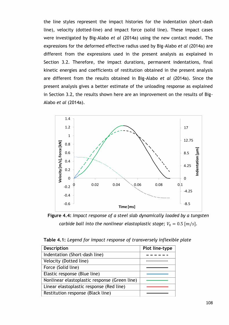
108

-8.5

-4.25

0

4.25

8.5

12.75

17

-0.6

-0.4

-0.2

0

0.2

0.4

0.6

0.8

1

1.2

1.4

0 0.02 0.04 0.06 0.08 0.1

Ind

en

tati

on

[μm

]

Ve

loci

ty [m

/s],

Fo

rce

[kN

]

Time [ms]

the line styles represent the impact histories for the indentation (short-dash

line), velocity (dotted-line) and impact force (solid line). These impact cases

were investigated by Big-Alabo et al (2014a) using the new contact model. The

expressions for the deformed effective radius used by Big-Alabo et al (2014a) are

different from the expressions used in the present analysis as explained in

Section 3.2. Therefore, the impact durations, permanent indentations, final

kinetic energies and coefficients of restitution obtained in the present analysis

are different from the results obtained in Big-Alabo et al (2014a). Since the

present analysis gives a better estimate of the unloading response as explained

in Section 3.2, the results shown here are an improvement on the results of Big-

Alabo et al (2014a).

Figure 4.4: Impact response of a steel slab dynamically loaded by a tungsten

carbide ball into the nonlinear elastoplastic stage; 𝑉0 = 0.5 [𝑚/𝑠].

Table 4.1: Legend for impact response of transversely inflexible plate

Description Plot line-type

Indentation (Short-dash line)

Velocity (Dotted line)

Force (Solid line)

Elastic response (Blue line)

Nonlinear elastoplastic response (Green line)

Linear elastoplastic response (Red line)

Restitution response (Black line)

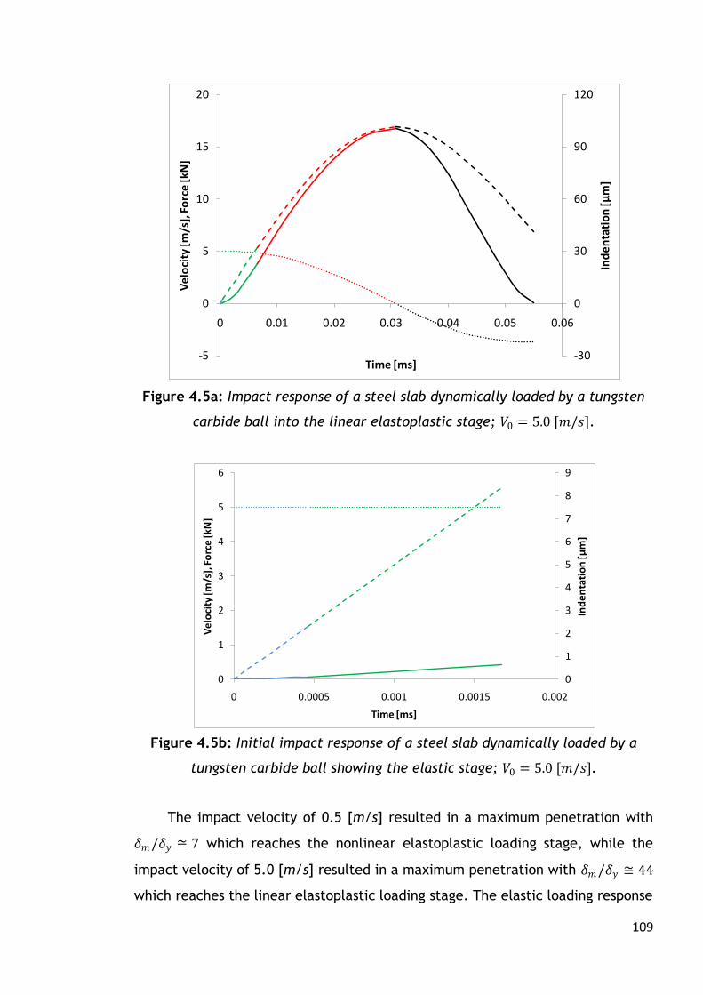
109

0

1

2

3

4

5

6

7

8

9

0

1

2

3

4

5

6

0 0.0005 0.001 0.0015 0.002

Ind

en

tati

on

[μm

]

Ve

loci

ty [m

/s],

Fo

rce

[kN

]

Time [ms]

-30

0

30

60

90

120

-5

0

5

10

15

20

0 0.01 0.02 0.03 0.04 0.05 0.06

Ind

en

tati

on

[μm

]

Ve

loci

ty [m

/s],

Fo

rce

[kN

]

Time [ms]

Figure 4.5a: Impact response of a steel slab dynamically loaded by a tungsten

carbide ball into the linear elastoplastic stage; 𝑉0 = 5.0 [𝑚/𝑠].

Figure 4.5b: Initial impact response of a steel slab dynamically loaded by a

tungsten carbide ball showing the elastic stage; 𝑉0 = 5.0 [𝑚/𝑠].

The impact velocity of 0.5 [m/s] resulted in a maximum penetration with

𝛿𝑚/𝛿𝑦 ≅ 7 which reaches the nonlinear elastoplastic loading stage, while the

impact velocity of 5.0 [m/s] resulted in a maximum penetration with 𝛿𝑚/𝛿𝑦 ≅ 44

which reaches the linear elastoplastic loading stage. The elastic loading response

110

0

0.001

0.002

0.003

0.004

0.005

0.006

0.007

0.008

0 0.02 0.04 0.06 0.08 0.1

Ene

rgy

[J]

Time [ms]

is seen to be visible when 𝑉0 = 0.5 [𝑚/𝑠] (Figure 4.4), and cannot be neglected

without introducing considerable errors in the estimation of the impact histories.

When 𝑉0 = 5.0 [𝑚/𝑠] the purely elastic response is barely noticeable compared to

the rest of the loading response (Figure 4.5a) and can be neglected. Figure 4.5b

shows the initial response when 𝑉0 = 5.0 [𝑚/𝑠] and reveals that the elastic

response has a negligible influence on the loading response since the initial

impact velocity barely changes at the end of the elastic loading response

(𝑉𝑦 = 4.99976[𝑚/𝑠]).


steel slab for 𝑉0 = 0.5 [𝑚/𝑠]. Kinetic energy: dash-dot line; Work done: short-

dash line.

The evolution of the kinetic energy of the impactor and work done on the

target by the impact force, in the loading and restitution stages, for initial

impact velocities of 0.5 [m/s] and 5.0 [m/s] are shown in Figures 4.6 and 4.7

respectively. In Figure 4.6, 13.8% of the initial KE of the impactor is dissipated

as plastic work whereas 45.9% is dissipated in Figure 4.7. The implication is that

increasing the initial impact velocity results in the dissipation of more of the

impactor’s initial KE as non-recoverable plastic work. This observation agrees

with the finding of Christoforou and Yigit (1998a) that a half-space impact

response is strongly influenced by the normalised impact velocity. Other results

for the impact response of the steel slab are summarised in Table 4.2, and the

111

0

0.1

0.2

0.3

0.4

0.5

0.6

0.7

0.8

0 0.01 0.02 0.03 0.04 0.05 0.06

Ene

rgy

[J]

Time [ms]

0.6

0.65

0.7

0.75

0.8

0.85

0.9

0.95

1

0 2 4 6 8 10

Co

eff

icie

nt o

f re

stit

uti

on

[-]

Impact velocity [m/s]

variation of the coefficient of restitution with initial impact velocity is shown in

Figure 4.8.


steel for 𝑉0 = 5[𝑚/𝑠]. Kinetic energy: dash-dot line; Work done: short-dash line.

Figure 4.8: Coefficient of restitution for impact of tungsten carbide ball on a

mild steel slab.

112

Table 4.2: Results of the impact response of steel

4.3 Algorithm for the solution of the impact model of

transversely inflexible rectangular plates

The impact response of a transversely inflexible plate (half-space) has been

modelled using the new contact model presented in Section 3.2. Solutions of the

impact models (equations 4.8 – 4.12) have been obtained by direct numerical

integration. The new contact model uses Meyer-type compliance models to

estimate the force during the loading and unloading stages of an impact event.

Half-space impact models in which the impact force is estimated by Meyer-type

compliance models can be readily solved by numerical integration (Goldsmith,

2001). The case is different when compliance models that cannot be expressed

in terms of Meyer’s law are used to estimate the impact force. This is because

the convergence of a conventional numerical scheme is not always guaranteed in

this context (Big-Alabo et al, 2014a).

Meyer’s law is generally regarded as the canonical form (i.e. standard

form) for most static contact models (Goldsmith, 2001). Yet, many existing

elastoplastic contact loading models cannot be expressed in terms of Meyer’s

law (Stronge, 2000a, Li et al, 2002; Jackson and Green, 2005; Brake, 2012). This

may explain why the application of these models to estimate the indentation,

velocity and force histories during half-space impact do not appear in the

literature despite their wide use for static indentation analyses. Therefore,

there is a need to develop either Meyer-type compliance models for the

elastoplastic loading regime (which has been done in Section 3.2) or more

efficient solution algorithms that could be used to solve the nonlinear models of

an elastoplastic half-space impact irrespective of the compliance model that has

been used to estimate the impact force.

Impact parameters Results

𝑉0 = 0.5[𝑚/𝑠] 𝑉0 = 5.0[𝑚/𝑠]

Impact duration [µs] 90.41 55.31

Time at maximum indentation [µs] 46.76 30.72

Permanent indentation [µm] 2.05 40.18

Maximum indentation [µm] 16.10 101.62

Maximum impact force [kN] 1.24 16.73

Final rebound velocity [m/s] 0.46 3.68

Coefficient of restitution [-] 0.93 0.74

113

Goldsmith (2001) used a small-increment numerical integration scheme

based on discretisation of the nonlinear force in the time-domain to obtain the

impact histories of an elastic impact from the nonlinear integral form of

equation (4.8). The computational effort and stability of this scheme is a

function of the nature of the nonlinearity in the differential equation and the

time-increment used. Abrate (1998) used the Newmark time integration scheme

for the solution of the impact response of an elastic half-space. The Newmark

scheme is a direct numerical integration scheme that involves discretisation of

the displacement, velocity, and acceleration in the time-domain. In order to

ensure convergence of the solution the Newmark scheme normally requires the

application of a fine-tuned time increment and involves many iteration steps.

Majeed et al (2012) used a nonlinear finite element method to obtain the force-

time history of an elastoplastic half-space impact; the finite element method

results were found to be in good agreement with the results obtained from the

simulation of equation (4.7) using their contact model. Also, numerical

integration solvers in computational software packages such as the NDSolve

function in MathematicaTM can be used to solve equation (4.7) when 𝐹 is a

nonlinear function of 𝛿 as demonstrated in Figures 4.4 – 4.7. The NDSolve

function solves differential equations numerically using an optimised routine

that automatically selects an integration method from a list of embedded

conventional methods such that convergence and computational efficiency are

ensured. Given that the NDSolve function uses conventional numerical methods

(Wolfram Research Inc., 2012) e.g. explicit Runge-Kutta, implicit Runge-Kutta,

and predictor-corrector Adams method, the issues of stability and convergence

inherent in these methods spring-up sometimes in the output of the function.

Consequently, the NDSolve function does not always converge on a solution in all

cases.

The problem with the finite element method and existing numerical

integration approaches is that they are conditionally stable, often complicated,

and usually require a large number of iterations to obtain accurate results and

are therefore often difficult to verify by means of hand calculation. In this

section, a new iterative solution algorithm called the Force-Indentation

Linearisation Method (FILM) is presented. The FILM uses closed-form solutions

derived from piecewise linearisation of the nonlinear impact force to determine

the impact histories of a half-space impact. In contrast to the conventional

114

numerical schemes in which key variables are discretised in the time-domain,

the FILM discretises the impact force with respect to indentation depth. The

limitations associated with the numerical methods and finite element methods

as stated above are completely eliminated by the FILM.

The FILM was applied by Big-Alabo et al (2014b) to determine the complete

impact histories for both elastic and elastoplastic impact events in which the

contact model of Majeed et al (2012) was used to estimate the impact force of

the elastoplastic impact. The study showed that the results of the FILM solution

matched results obtained by direct numerical integration. In this section, the

FILM has been generalised for the solution of half-space impact models in which

the impact force is estimated from canonical or non-canonical compliance

models. First, the general concept of the FILM is discussed and thereafter the

concept is applied to formulate solutions for impact models that are based on

canonical and non-canonical compliance models. Finally, the implications for

applying the FILM to solve impact models of transversely flexible plates are

discussed.

4.3.1 Concept of the FILM

Closed-form solutions of a half-space impact response can be obtained

when a linearised force-indentation relationship is used. Hence, if the nonlinear

force-indentation curve between the initial and end states of an impact stage is

approximated using several line segments joined end to start, then each line

segment representing a linear force-indentation relationship gives a closed-form

solution that is only applicable to the range of indentation it covers. The slopes

of the line segments represent linearised contact stiffnesses, and the slopes

change between the initial and end states of the impact stage considered. This

changing slope results in a changing force-indentation relationship that can be

used to update the solution from one piecewise linearisation to the next.

Figures 4.9 a-c shows a typical nonlinear force-indentation relationship

with various approximations. Obviously, Figure 4.9c with three line segments

gives a better description of the impact histories compared to Figures 4.9a and

4.9b. The implication is that increasing the number of line segments produces a

better approximation of the nonlinear force-indentation curve and gives a more

accurate estimation of the impact history.

115

δ

F

δ

F

δ

F

(a) (b) (c)

Figure 4.9: Linear discretisation of nonlinear force indentation relationship (a)

one line (b) two lines (c) three lines.

The FILM produces closed-form solutions for the impact response for each

piecewise linearisation of the nonlinear impact force. The closed-form solutions

for each piecewise linearisation do not oscillate or diverge and this makes the

FILM inherently stable unlike other commonly used numerical methods

(Goldsmith, 2001; Abrate, 1998) and the finite element methods.

Let us assume that 𝐹(𝛿) is a nonlinear function of 𝛿 as shown in Figure 4.10

and 𝐹𝑖 = 𝐹(𝛿𝑖) where 𝑖 represents any point on the nonlinear force-indentation

relationship. Then from Figure 4.10, 𝐹01 = slope of 01 × (𝛿01 − 𝛿0) + 𝐹0 where

𝐹01 is the linearised force for the segment of 𝐹 𝛿 between point 0 and point 1.

Hence,

𝐹01 = 𝐹1 − 𝐹0

𝛿1 − 𝛿0

𝛿01 − 𝛿0 + 𝐹0 =𝐹(𝛿1) − 𝐹(𝛿0)

𝛿1 − 𝛿0

𝛿01 − 𝛿0 + 𝐹 𝛿0 (4.13)

Similarly,

𝐹12 = 𝐹 𝛿2 − 𝐹 𝛿1

𝛿2 − 𝛿1(𝛿12 − 𝛿1) + 𝐹(𝛿1) (4.14)

And generally,

𝐹𝑟𝑠 = 𝐹 𝛿𝑠 − 𝐹 𝛿𝑟

𝛿𝑠 − 𝛿𝑟(𝛿𝑟𝑠 − 𝛿𝑟) + 𝐹 𝛿𝑟 (4.15)

where 𝑟 = 0,1, 2, 3,… ,𝑛 − 1 and 𝑠 = 𝑟 + 1 are the initial and end states of each

segment respectively. During unloading 𝑟 = 𝑛,𝑛 − 1, 𝑛 − 2,… ,2,1 are the initial

states while 𝑠 = 𝑟 − 1 are the end states. 𝐹𝑟𝑠 is the linearised force for each

segment and it can be written as:

𝐹𝑟𝑠 = 𝐾𝑟𝑠 𝛿𝑟𝑠 − 𝛿𝑟 + 𝐹 𝛿𝑟 (4.16𝑎)

116

δ

F1

δ1

F2

F0

δ2 δe

1

0

2 A

B

E Fe

C

δ0

F

where

𝐾𝑟𝑠 =𝐹(𝛿𝑠) − 𝐹(𝛿𝑟)

𝛿𝑠 − 𝛿𝑟 (4.16𝑏)

Figure 4.10: Tri-linear approximation of a general nonlinear impact force used

to demonstrate the concept of the FILM.

Supposing each segment has an equal indentation range i.e. ∆𝛿 is constant,

then 𝛿𝑟 can be expressed for 𝑛 segments as:

𝛿𝑟 = 𝛿0 + 𝑟 𝛿𝑒 − 𝛿0 /𝑛 (4.17)

When equation (4.16a) is substituted in equation (4.7), a linear differential

equation is obtained from which closed-form solutions can be derived for each

segment. This simple concept, combined with the energy balance principle (see

Section 3.3.3.1), can be used to derive the complete solution of a half-space

impact irrespective of the nature of nonlinearity in the compliance model used

to estimate the impact force.

4.3.2 Solution of half-space impact modelled based on a canonical

compliance law using the FILM

As mentioned earlier, Meyer’s law is the standard form for static contact

models. Meyer’s law can be expressed as (Goldsmith, 2001):

𝐹 = 𝐾𝑐𝛿𝑞 (4.18)

117

where 𝐾𝑐 is the contact stiffness and 𝑞 ≥ 1 is a number defining the power law

relationship between the contact force and indentation. For example 𝐾𝑐 is equal

to the Hertzian contact stiffness (see equation 3.31) and 𝑞 = 3/2 during elastic

impact. A more general form of Meyer’s law, incorporating post-yield effects can

be written as:

𝐹 = 𝐾𝑐 𝛿 − 𝛿0 𝑞 + 𝐹0 (4.19)

where 𝛿0 and 𝐹0 are the indentation and contact force at the onset of a loading

or unloading regime. During the elastic impact response 𝛿0 = 0 and 𝐹0 = 0, while

for post-yield impact response, 𝛿0 ≠ 0 and 𝐹0 ≠ 0. Therefore, the model for a

half-space impact, governed by a canonical compliance law that accounts for

post-yield effects, can be written as:

𝑚𝑖𝛿 + 𝐾𝑐 𝛿 − 𝛿0 𝑞 + 𝐹0 = 0 (4.20)

The FILM is only applied when 𝑞 > 1 and equation (4.20) is nonlinear. If 𝑞 = 1,

then equation (4.20) is linear and closed-form solutions can be obtained directly

without need for the FILM or any other numerical integration scheme.

Using equation (4.19) in equation (4.15),

𝐹𝑟𝑠 = 𝐾𝑐 𝛿𝑠 − 𝛿0

𝑞 − 𝐾𝑐 𝛿𝑟 − 𝛿0 𝑞

𝛿𝑠 − 𝛿𝑟 𝛿𝑟𝑠 − 𝛿𝑟 + 𝐾𝑐 𝛿𝑟 − 𝛿0

𝑞 + 𝐹 𝛿0 (4.21)

From equation (4.17),

𝛿𝑠 = 𝛿𝑟+1 = 𝛿𝑟 + 𝛿𝑒 − 𝛿0 /𝑛 (4.22)

Note that 𝛿𝑒 is the indentation at the end of the loading or unloading stage

considered (see Figure 4.10), and 𝛿𝑒 can be obtained from the compliance model

used or the energy balance algorithm (see Figure 3.10) when it is equal to the

maximum indentation. Substituting equation (4.22) in equation (4.21), and after

algebraic simplifications, the linearised contact force for each discretisation can

be written as:

𝐹𝑟𝑠 = 𝐾𝑟𝑠 𝛿𝑟𝑠 − 𝛿𝑟 + 𝐾𝑐 𝛿𝑟 − 𝛿0 𝑞 + 𝐹0 (4.23)

where

𝐾𝑟𝑠 = 𝑛𝐾𝑐 𝛿𝑒 − 𝛿0 𝑞−1

𝑠

𝑛

3/2

− 𝑟

𝑛

3/2

(4.24)

Substituting equation (4.23) in equation (4.7), the governing equation for the

impact response of each discretisation is given by:

𝑚𝑖𝛿 𝑟𝑠 + 𝐾𝑟𝑠𝛿𝑟𝑠 = 𝐾𝑟𝑠𝛿𝑟 − 𝐾𝑐 𝛿𝑟 − 𝛿0 𝑞 − 𝐹0 (4.25)

Equation (4.25) is a non-homogeneous linear differential equation and the

complete solution can be readily obtained as:

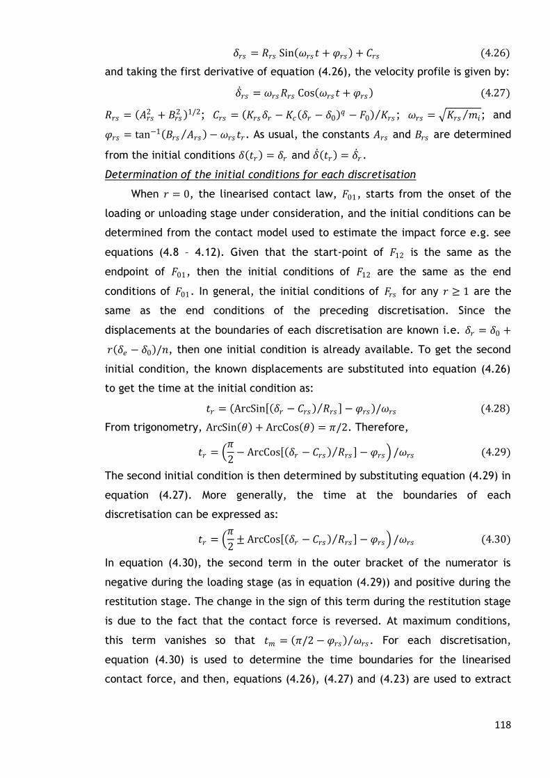
118

𝛿𝑟𝑠 = 𝑅𝑟𝑠 Sin 𝜔𝑟𝑠𝑡 + 𝜑𝑟𝑠 + 𝐶𝑟𝑠 (4.26)

and taking the first derivative of equation (4.26), the velocity profile is given by:

𝛿 𝑟𝑠 = 𝜔𝑟𝑠𝑅𝑟𝑠 Cos 𝜔𝑟𝑠𝑡 + 𝜑𝑟𝑠 (4.27)

𝑅𝑟𝑠 = 𝐴𝑟𝑠2 + 𝐵𝑟𝑠

2 1/2; 𝐶𝑟𝑠 = 𝐾𝑟𝑠𝛿𝑟 − 𝐾𝑐 𝛿𝑟 − 𝛿0 𝑞 − 𝐹0 𝐾𝑟𝑠 ; 𝜔𝑟𝑠 = 𝐾𝑟𝑠 𝑚𝑖 ; and

𝜑𝑟𝑠 = tan−1 𝐵𝑟𝑠 𝐴𝑟𝑠 − 𝜔𝑟𝑠 𝑡𝑟. As usual, the constants 𝐴𝑟𝑠 and 𝐵𝑟𝑠 are determined

from the initial conditions 𝛿 𝑡𝑟 = 𝛿𝑟 and 𝛿 𝑡𝑟 = 𝛿 𝑟.

Determination of the initial conditions for each discretisation

When 𝑟 = 0, the linearised contact law, 𝐹01, starts from the onset of the

loading or unloading stage under consideration, and the initial conditions can be

determined from the contact model used to estimate the impact force e.g. see

equations (4.8 – 4.12). Given that the start-point of 𝐹12 is the same as the

endpoint of 𝐹01, then the initial conditions of 𝐹12 are the same as the end

conditions of 𝐹01. In general, the initial conditions of 𝐹𝑟𝑠 for any 𝑟 ≥ 1 are the

same as the end conditions of the preceding discretisation. Since the

displacements at the boundaries of each discretisation are known i.e. 𝛿𝑟 = 𝛿0 +

𝑟 𝛿𝑒 − 𝛿0 /𝑛, then one initial condition is already available. To get the second

initial condition, the known displacements are substituted into equation (4.26)

to get the time at the initial condition as:

𝑡𝑟 = ArcSin 𝛿𝑟 − 𝐶𝑟𝑠 𝑅𝑟𝑠 − 𝜑𝑟𝑠 /𝜔𝑟𝑠 (4.28)

From trigonometry, ArcSin 휃 + ArcCos 휃 = 𝜋/2. Therefore,

𝑡𝑟 = 𝜋

2− ArcCos 𝛿𝑟 − 𝐶𝑟𝑠 𝑅𝑟𝑠 − 𝜑𝑟𝑠 /𝜔𝑟𝑠 (4.29)

The second initial condition is then determined by substituting equation (4.29) in

equation (4.27). More generally, the time at the boundaries of each

discretisation can be expressed as:

𝑡𝑟 = 𝜋

2± ArcCos 𝛿𝑟 − 𝐶𝑟𝑠 𝑅𝑟𝑠 − 𝜑𝑟𝑠 /𝜔𝑟𝑠 (4.30)

In equation (4.30), the second term in the outer bracket of the numerator is

negative during the loading stage (as in equation (4.29)) and positive during the

restitution stage. The change in the sign of this term during the restitution stage

is due to the fact that the contact force is reversed. At maximum conditions,

this term vanishes so that 𝑡𝑚 = 𝜋/2 − 𝜑𝑟𝑠 𝜔𝑟𝑠 . For each discretisation,

equation (4.30) is used to determine the time boundaries for the linearised

contact force, and then, equations (4.26), (4.27) and (4.23) are used to extract

119

data points for the indentation, velocity and contact force histories within the

time boundaries.

The above FILM solution, for a half-space impact response modelled based

on a canonical compliance law, is demonstrated using the tungsten carbide –

mild steel impact discussed in Section 4.2. The material properties of the impact

system remain the same, while the impact velocity used in the present

investigation is 0.25 [m/s]. It is recalled that an impact velocity of 0.5 [m/s]

produced a maximum indentation that is located in the nonlinear elastoplastic

loading regime. Hence, the impact stages involved for an impact velocity of 0.25

[m/s] are: elastic loading, nonlinear elastoplastic loading and elastic unloading;

all of which are modelled with nonlinear canonical compliance models according

to the new contact model. This means that the FILM can be applied to all the

impact stages involved.

Application of the FILM to the solution of the elastic loading response

The elastic loading response covers the indentation range 0 ≤ 𝛿 ≤ 𝛿𝑦 .

Based on the new contact model 𝛿0 = 0; 𝐹0 = 0; 𝐾𝑐 = 𝐾𝑕 ; 𝑞 = 3/2; and 𝛿𝑒 = 𝛿𝑦 .

From the FILM solution, the following changes apply to the elastic loading

response.

𝐹𝑟𝑠 = 𝐾𝑟𝑠 𝛿𝑟𝑠 − 𝛿𝑟 + 𝐾𝑕𝛿𝑟3/2

; 𝐾𝑟𝑠 = 𝑛𝐾𝑕𝛿𝑦1/2 𝑠/𝑛 3/2 − 𝑟/𝑛 3/2 ; 𝛿𝑟 = 𝑟𝛿𝑦/𝑛;

𝐶𝑟𝑠 = 𝐾𝑟𝑠𝛿𝑟 − 𝐾𝑕𝛿𝑟3/2 𝐾𝑟𝑠 .

Application of the FILM to the solution of the nonlinear elastoplastic loading

response

The nonlinear elastoplastic loading response covers the indentation range

𝛿𝑦 ≤ 𝛿 ≤ 𝛿𝑚 . The maximum indentation, 𝛿𝑚 , is estimated using the energy-

balance algorithm in Figure 3.10. Following this algorithm the maximum

indentation for the present impact event is estimated from:

1

2𝑚𝑖𝑉0

2 = 0.4𝐾𝑕𝛿𝑦5 2 + 0.4𝐾𝑕 𝛿𝑚 − 𝛿𝑦

5 2 + 𝐾𝑕𝛿𝑦

3 2 𝛿𝑚 − 𝛿𝑦 (4.31)

Based on the new contact model, 𝛿0 = 𝛿𝑦 ; 𝐹0 = 𝐹𝑦 = 𝐾𝑕𝛿𝑦3/2

; 𝐾𝑐 = 𝐾𝑕; 𝑞 = 3/2;

and 𝛿𝑒 = 𝛿𝑚 . From the FILM solution, the following changes apply to the

nonlinear elastoplastic loading response.

𝐹𝑟𝑠 = 𝐾𝑟𝑠 𝛿𝑟𝑠 − 𝛿𝑟 + 𝐾𝑕 𝛿𝑟 − 𝛿𝑦 3/2

+ 𝐹𝑦;

120

𝐾𝑟𝑠 = 𝑛𝐾𝑕 𝛿𝑚 − 𝛿𝑦 1/2

𝑠/𝑛 3/2 − 𝑟/𝑛 3/2 ;

𝛿𝑟 = 𝛿𝑦 + 𝑟 𝛿𝑚 − 𝛿𝑦 /𝑛; and 𝐶𝑟𝑠 = 𝐾𝑟𝑠𝛿𝑟 − 𝐾𝑕 𝛿𝑟 − 𝛿𝑦 3/2

− 𝐹𝑦 𝐾𝑟𝑠 .

Application of the FILM to the solution of the unloading response

The unloading response covers the indentation range 𝛿𝑓 ≤ 𝛿 ≤ 𝛿𝑚 . From the

new contact model 𝛿0 = 𝛿𝑓 ; 𝐹0 = 0; 𝐾𝑐 = 𝐾𝑢; 𝑞 = 3/2; and 𝛿𝑒 = 𝛿𝑚 . From the

FILM solution, the following changes apply to the unloading response.

𝐹𝑟𝑠 = 𝐾𝑟𝑠 𝛿𝑟𝑠 − 𝛿𝑟 + 𝐾𝑢 𝛿𝑟 − 𝛿𝑓 3/2

;

𝐾𝑟𝑠 = 𝑛𝐾𝑢 𝛿𝑚 − 𝛿𝑓 1 2

𝑠/𝑛 3/2 − 𝑟/𝑛 3/2 ;

𝛿𝑟 = 𝛿𝑓 + 𝑟 𝛿𝑚 − 𝛿𝑓 /𝑛; and 𝐶𝑟𝑠 = 𝐾𝑟𝑠𝛿𝑟 − 𝐾𝑢 𝛿𝑟 − 𝛿𝑓 3/2

𝐾𝑟𝑠 .

Note that the unloading response has been discretised from the bottom-up,

which is why the onset is at the point 𝛿𝑓 , 0 instead of 𝛿𝑚 ,𝐹𝑚 as might be

expected. The bottom-up discretisation has been used for mathematical

convenience and it gives the same results as would have been obtained if the

discretisation was done from the top-down and the onset is at 𝛿𝑚 ,𝐹𝑚 .

Additionally, the sign change of the middle term in equation (4.30) during

unloading makes the bottom-up solution to be consistent with the top-down

solution.

The above FILM solution was implemented in a customised Mathematica™

code (see appendix B.1) that was used to estimate the impact response of the

tungsten carbide – mild steel impact system. The code was run using five

discretisations in each of the impact stages and the close-form solutions derived

for each discretisation were used to extract data points for plotting the impact

histories. Figure 4.11 shows the results of the FILM approach compared with

numerical integration results obtained using the NDSolve function; the results

are in excellent agreement.

121

0

1

2

3

4

5

6

7

8

9

10

-0.3

-0.2

-0.1

0

0.1

0.2

0.3

0.4

0.5

0.6

0 0.02 0.04 0.06 0.08 0.1 0.12

Ind

en

tati

on

[µm

]

Ve

loci

ty [m

/s],

Fo

rce

[kN

]

Time [ms]

F

δ

dδ/dt


integration method. Lines – FILM solution; Markers – numerical solution. See

Table 4.1 for line colour definition.

4.3.3 Solution of half-space impact modelled based on a non-

canonical compliance law using the FILM

Non-canonical compliance models are those that cannot be expressed in

terms of equation (4.19); examples include the elastoplastic loading models of

Stronge (2000a) and Brake (2012). Conventional numerical integration schemes

do not guarantee convergent solutions for half-space impact models in which

non-canonical compliance models are used to estimate the impact force (Big-

Alabo et al, 2014a). This is because of the more complex nonlinear form in

which such contact models are expressed. The FILM is shown here to be a

solution algorithm that guarantees convergent solutions when non-canonical

contact models are used to estimate the impact force of a half-space impact.

Interestingly, the FILM approach produces the solution with the same relative

ease as it does with a half-space impact model based on a canonical contact

model. This is because the number of discretisations need not be increased to

guarantee convergent solutions even when a more complex contact model is

used to estimate the impact force. To demonstrate this, the FILM algorithm is

applied to solve the tungsten-carbide impact problem discussed in Section 4.3.2

when the contact model of Stronge (2000a) is used to estimate the impact force.

122

The contact model of Stronge (2000a) was discussed in Section 3.1.1. The

elastic loading regime was modelled using the Hertz contact model, while the

model for the elastoplastic loading regime used a logarithmic function of

indentation depth. The model for the unloading regime is a modified form of the

Hertz model that accounts for the effect of permanent indentation. All three

regimes are modelled using nonlinear force-indentation relationships and

therefore, the corresponding impact response models are nonlinear and would

normally require numerical solution. In the following analysis, the FILM approach

is applied to determine the impact histories when Stronge’s contact model is

used to estimate the impact force.

Application of the FILM to the solution of the elastic loading response

The FILM solution for the elastic loading stage of the impact response is the

same as in Section 4.3.2 since Stronge (2000a) also used the Hertz model to

estimate the elastic impact response.

Application of the FILM to the solution of the nonlinear elastoplastic loading

response

For convenience Stronge’s elastoplastic loading model is restated here.

𝐹 = 𝐹𝑦 2𝛿

𝛿𝑦− 1 1 +

1

3.3𝑙𝑛

2𝛿

𝛿𝑦− 1 𝛿𝑦 ≤ 𝛿 ≤ 𝛿𝑝 (4.32)

The nonlinear elastoplastic loading response covers the indentation range

𝛿𝑦 ≤ 𝛿 ≤ 𝛿𝑚 . Again, the maximum indentation, 𝛿𝑚 , is estimated using the

energy-balance principle. Using equation (4.32) Stronge (2000a) derived the

indentation work from the beginning of the elastic loading to any point in the

elastoplastic loading regime as:

𝑊 = 𝑊𝑦 0.47 + 0.53 2𝛿

𝛿𝑦− 1

2

+ 0.189 2𝛿

𝛿𝑦− 1

2

𝑙𝑛 2𝛿

𝛿𝑦− 1 (4.33)

where 𝑊𝑦 = 0.4𝐾𝑕𝛿𝑦5/2

. Therefore, the maximum indentation of an elastoplastic

impact can be determined based on Stronge’s model by equating the

deformation work in equation (4.33) to the initial impact energy as follows:

1

2𝑚𝑖𝑉0

2 = 𝑊𝑦 0.47 + 0.53 2𝛿𝑚𝛿𝑦

− 1

2

+ 0.189 2𝛿𝑚𝛿𝑦

− 1

2

𝑙𝑛 2𝛿𝑚𝛿𝑦

− 1 (4.34)

Based on Stronge’s elastoplastic model, 𝛿0 = 𝛿𝑦 ; 𝐹0 = 𝐹𝑦 = 𝐾𝑕𝛿𝑦3/2

; and 𝛿𝑒 = 𝛿𝑚 .

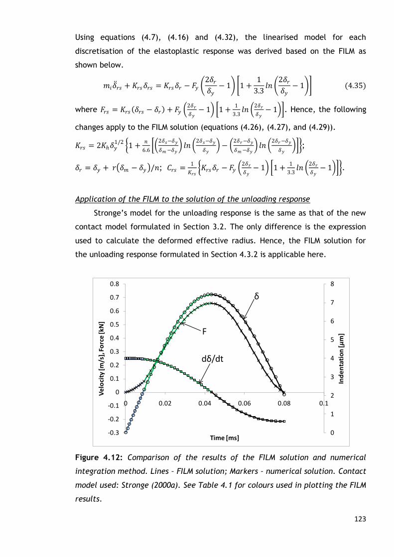
123

0

1

2

3

4

5

6

7

8

-0.3

-0.2

-0.1

0

0.1

0.2

0.3

0.4

0.5

0.6

0.7

0.8

0 0.02 0.04 0.06 0.08 0.1

Ind

en

tati

on

[μm

]

Ve

loci

ty [m

/s],

Fo

rce

[kN

]

Time [ms]

dδ/dt

F

δ

Using equations (4.7), (4.16) and (4.32), the linearised model for each

discretisation of the elastoplastic response was derived based on the FILM as

shown below.

𝑚𝑖𝛿 𝑟𝑠 + 𝐾𝑟𝑠𝛿𝑟𝑠 = 𝐾𝑟𝑠𝛿𝑟 − 𝐹𝑦 2𝛿𝑟𝛿𝑦

− 1 1 +1

3.3𝑙𝑛

2𝛿𝑟𝛿𝑦

− 1 (4.35)

where 𝐹𝑟𝑠 = 𝐾𝑟𝑠 𝛿𝑟𝑠 − 𝛿𝑟 + 𝐹𝑦 2𝛿𝑟

𝛿𝑦− 1 1 +

1

3.3𝑙𝑛

2𝛿𝑟

𝛿𝑦− 1 . Hence, the following

changes apply to the FILM solution (equations (4.26), (4.27), and (4.29)).

𝐾𝑟𝑠 = 2𝐾𝑕𝛿𝑦1/2 1 +

𝑛

6.6

2𝛿𝑠−𝛿𝑦

𝛿𝑚−𝛿𝑦 𝑙𝑛

2𝛿𝑠−𝛿𝑦

𝛿𝑦 −

2𝛿𝑟−𝛿𝑦

𝛿𝑚−𝛿𝑦 𝑙𝑛

2𝛿𝑟−𝛿𝑦

𝛿𝑦 ;

𝛿𝑟 = 𝛿𝑦 + 𝑟 𝛿𝑚 − 𝛿𝑦 /𝑛; 𝐶𝑟𝑠 =1

𝐾𝑟𝑠 𝐾𝑟𝑠𝛿𝑟 − 𝐹𝑦

2𝛿𝑟

𝛿𝑦− 1 1 +

1

3.3𝑙𝑛

2𝛿𝑟

𝛿𝑦− 1 .

Application of the FILM to the solution of the unloading response

Stronge’s model for the unloading response is the same as that of the new

contact model formulated in Section 3.2. The only difference is the expression

used to calculate the deformed effective radius. Hence, the FILM solution for

the unloading response formulated in Section 4.3.2 is applicable here.


integration method. Lines – FILM solution; Markers – numerical solution. Contact

model used: Stronge (2000a). See Table 4.1 for colours used in plotting the FILM

results.

124

The FILM solution derived above for the various impact stages was

implemented in a customised Mathematica™ code and used to estimate the

impact response of the tungsten carbide – mild steel impact case study. The

code was run using five discretisations in each of the impact stages and the

closed-form solutions derived for each discretisation were used to extract data

points for plotting the impact histories. Figure 4.12 shows the results of the FILM

approach in comparison with results obtained by numerical integration using the

NDSolve function. Some key results of the tungsten carbide – mild steel impact

response based on the newly proposed contact model and Stronge’s contact

model are given in Table 4.3. Results reveal that the contact model used to

estimate the impact force can greatly influence the prediction of the impact

response. In view of the fact that the new contact model has been validated

using published static and dynamic indentation test results (see Section 3.3), the

predicted impact response based on the new contact model is considered to be

reliable.

Table 4.3: Tungsten carbide – mild steel impact response results obtained using

FILM

4.3.4 Implications of applying the FILM approach for the solution

of the impact response of transversely flexible plates

During normal impact of transversely inflexible plates, which can be

modelled using half-space assumptions, the flexural oscillations are negligible.

The impact energy is primarily used for local indentation of the plate when other

mechanisms of energy dissipation such as elastic waves and friction can be

neglected, and the impact force can be estimated using quasi-static indentation

Impact parameters

Results

New contact

model

Stronge’s

contact model

Impact duration [µs] 105.14 79.78

Time at maximum indentation [µs] 55.57 43.24

Permanent indentation [µm] 1.78 2.09

Maximum indentation [µm] 9.45 7.44

Maximum impact force [N] 513.41 657.29

Final rebound velocity [m/s] 0.23 0.22

Coefficient of restitution [-] 0.92 0.87

125

models (Johnson, 1985). The implication is that the impactor velocity is zero at

maximum conditions. These features of a half-space impact allow for the use of

the energy-balance principle in estimating the maximum indentation during

impact loading (Abrate, 1998). For normal impact of transversely flexible plates

the flexural oscillations of the plate cannot be neglected, and the interactions

between the flexural oscillations and the local indentation determine the impact

response. This means that the vibration model of the plate and a compliance

model accounting for local indentation must be used in modelling the impact

response (see Section 4.4 for more details). The response is dynamic and

complex, making it impossible to use the energy-balance principle to determine

the maximum indentation for a transversely flexible plate impact (Abrate,

1998).

In order to determine the impact response using the FILM approach the

indentation and impact force at the end of the loading must be known. The end

conditions of the impact loading are used as the initial conditions and other

inputs for the unloading response. While it is possible to have this information

from the energy-balance principle in the case of a transversely inflexible plate

impact, it is not possible in the case of a transversely flexible plate impact.

However, the impact loading phase during a transversely flexible plate impact

ends when the impactor velocity is zero because the impact loading is due to the

deceleration of the impactor. If the end indentation of the impact loading is

chosen a priori, such that this assumed end indentation is definitely higher than

the actual end indentation, then the condition of zero impactor velocity can be

used as a test condition to determine the actual end of the impact loading. In

principle the maximum indentation of the corresponding elastic half-space

impact is always greater that the actual end indentation of the transversely

flexible plate impact and this can therefore be conveniently used as the

assumed end indentation.

The maximum indentation of a transversely flexible plate impact occurs

when the relative velocity of the impactor and the plate is zero. For impact

events in which the impact force does not oscillate, the condition of zero

relative velocity occurs only once and this is at the maximum indentation point.

Hence, the zero relative velocity condition is sufficient to determine the point

where the maximum indentation occurs when the impact force does not

oscillate. This does not mean that the zero relative velocity condition can be

126

used to determine the maximum indentation before implementing the FILM

approach. Rather, the zero relative velocity condition can only be used as a test

condition in the implementation of the FILM approach to know when the

maximum indentation is reached. The infinite plate impact is an example of an

impact event that is characterised by a non-oscillating impact force, and

therefore can be solved using the FILM.

In cases where the impact force oscillates, the zero relative velocity

condition occurs more than once, making it necessary to have another condition

to determine the maximum indentation point. Apparently, such a

complementary condition is not known. Hence, the zero relative velocity

condition is not sufficient to determine the maximum indentation when the

impact force oscillates. The oscillation of the impact force is due to the

influence of vibration waves reflected from the boundary. Thus, the FILM

approach is more difficult to implement for a transversely flexible plate impact

with an oscillating impact force. Therefore, the FILM approach is recommended

for transversely flexible plate impacts with non-oscillatory impact force i.e.

small mass impacts.

As explained above the FILM approach can be used to solve the infinite

plate model with slight modifications. To demonstrate this, an elastic impact

problem studied by Olsson (1992) is considered here. The material and

geometrical properties of the graphite/epoxy composite laminate plate and

steel impactor used by Olsson (1992) are given in Table 4.4. The infinite plate

model for an orthotropic composite plate is a single differential equation given

by (Chai and Zhu, 2011; Olsson, 1992)

𝛿 +1

8 𝜌𝐷𝐹 +

𝐹

𝑚𝑝= 0 (4.36)

where 𝜌𝑎 is the mass per unit area of the plate [𝑘𝑔/𝑚2], 𝐷 is the effective

mechanical bending stiffness of the plate [𝑁𝑚], 𝑚𝑖 is the mass of the impactor

[𝑘𝑔] and 𝐹 is the impact force [𝑁]. The effective stiffness is calculated as

𝐷 = [(𝐴 + 1)/2] 𝐷11𝐷22 where 𝐴 = 𝐷12 + 2𝐷66 / 𝐷11𝐷22. The 𝐷𝑖𝑗 constants are

bending stiffness constants that are calculated from the material properties of

the plate, as discussed in Section 2.5. The impact force can be estimated using a

static contact model and is a function of the local indentation i.e. 𝐹 = 𝐹(𝛿).

Hence, substituting an appropriate static contact model in equation (4.36) would

127

produce a differential equation in 𝛿(𝑡), the solution of which gives the local

indentation history. The local indentation is expressed as: 𝛿(𝑡) = 𝑤𝑖 𝑡 − 𝑤(𝑡)

where 𝑤𝑖 𝑡 and 𝑤 𝑡 are respectively the displacements of the impactor and the

plate at the point of impact. The displacement of the plate at the point of

impact is given by:

𝑤(𝑡) =1

8 𝜌𝐷 𝐹 𝜏 𝑡

𝑡0

𝑑𝜏 (4.37)

where 𝑡0 is the time at the onset of the impact stage considered, and 𝑡0 = 0 for

elastic impact.

The complete solution of the infinite plate impact model can be

determined once the local indentation history is obtained from the solution of

equation (4.36). The local indentation history is used to determine the impact

force history from the static contact model that was initially substituted into

equation (4.36), and the impact force so obtained is substituted into equation

(4.37) to determine the displacement of the plate at the point of impact.

Thereafter, the displacement of the impactor can be obtained from the solutions

of the local indentation and plate displacement. Also, the velocities of the

impactor and the plate can be obtained by differentiating the solutions of the

respective displacements.

Table 4.4: Properties of the steel –laminate impact system (Olsson, 1992)

Material properties

Graphite/epoxy (T300/934) composite plate: Lamination sequence =

[0/90/0/90/0]s; 𝜌 = 4.132 [𝑘𝑔/𝑚2]; 𝐷11 = 154.9 [𝑁𝑚]; 𝐷12 = 4.76 [𝑁𝑚]; 𝐷22 =

91.4 [𝑁𝑚]; 𝐷66 = 8.97 [𝑁𝑚]; 𝑕 = 2.69 [𝑚𝑚]; 𝐴 = 200 × 200 [𝑚𝑚2];

Impactor (Steel): 𝑚 = 8.3 [𝑔]; 𝑉0 = 3 [𝑚/𝑠]; 𝑅𝑖 = 6.35 [𝑚𝑚]

Other inputs: Effective contact modulus = 9.72 [𝐺𝑃𝑎]; 𝑅𝑡 = ∞

During elastic impact of transversely flexible composite plates, the Hertz

contact model can be used to estimate the impact force. Using the Hertz

contact model in equation (4.36) the model for elastic impact response is

derived thus:

𝛿 +3𝐾𝑕

16 𝜌𝐷𝛿1 2 𝛿 +

𝐾𝑕𝑚𝑝

𝛿3 2 = 0 (4.38)

128

The initial conditions are 𝛿 0 = 0 and 𝛿 0 = 𝑉0. Equation (4.38) is a nonlinear

differential equation and would normally require a numerical solution. Using the

FILM approach by substituting the linearised contact force for the Hertz contact

model (see Section 4.3.2) into equation (4.37), the impact response model for

each discretisation of the impact force can be derived as:

𝛿 𝑟𝑠 +𝐾𝑟𝑠

8 𝜌𝐷𝛿 𝑟𝑠 +

𝐾𝑟𝑠𝑚𝑝

𝛿𝑟𝑠 =𝐾𝑟𝑠𝛿𝑟 − 𝐾𝑕𝛿𝑟

3/2

𝑚𝑝 (4.39)

where 𝐾𝑟𝑠 = 𝑛𝐾𝑕𝛿𝑚1/2 𝑠/𝑛 3/2 − 𝑟/𝑛 3/2 ; 𝛿𝑟 = 𝑟𝛿𝑚/𝑛; 𝑟 = 0, 1, 2, 3,… ,𝑛 − 1;

𝑠 = 𝑟 + 1; and 𝑛 is the number of discretisations. Since the maximum indentation

of the infinite plate model cannot be determined from the onset as explained

above, the maximum indentation of the corresponding elastic half-space impact

is used and the zero relative velocity condition is tested for each linearisation to

determine the point when the actual maximum indentation is reached. This

maximum indentation is less than that of the corresponding elastic half-space

impact (Olsson, 1992). However, the impact loading ends when the impactor

velocity is zero. This second condition is also tested to determine the end of the

impact loading and to determine the initial conditions at the beginning of the

unloading stage.

Equation (4.39) can be rewritten as

𝛿 𝑟𝑠 + 2𝜆𝑟𝑠𝛿 𝑟𝑠 + 𝜔𝑟𝑠2 𝛿𝑟𝑠 = 𝑃𝑟𝑠 (4.40)

where 𝜆𝑟𝑠 = (1/16) 𝑚𝑝𝐾𝑟𝑠/𝜌𝐷; 𝜔𝑟𝑠 = 𝐾𝑟𝑠/𝑚𝑝; and 𝑃𝑟𝑠 = 𝐾𝑟𝑠𝛿𝑟 − 𝐾𝑕𝛿𝑟3/2 /𝑚𝑝

are the damping constant, circular frequency of the linearised response and

constant load respectively. Equation (4.40) describes the motion of an initially

excited damped oscillator with a constant load. The solution depends on the

value of the damping constant, 𝜆𝑟𝑠, i.e. whether the motion is under-damped,

critically-damped, or over-damped. The complete solutions to equation (4.40)

are comprised of the particular and homogeneous solutions for the different

cases of damping and are given as:

Under-damped 0 < 𝜆𝑟𝑠 < 1

𝛿𝑟𝑠 = 𝑅𝑟𝑠𝑒−𝜆𝑟𝑠𝜔𝑟𝑠 𝑡 Sin 𝜔𝑑𝑟𝑠 𝑡 + 𝜑𝑑𝑟𝑠 + 𝐶𝑟𝑠 (4.41)

Critically-damped 𝜆𝑟𝑠 = 1

𝛿𝑟𝑠 = 𝑒−𝜔𝑟𝑠 𝑡 𝐴𝑟𝑠 + 𝐵𝑟𝑠 𝑡 +𝐶𝑟𝑠 (4.42)

Over-damped 𝜆𝑟𝑠 > 1

129

𝛿𝑟𝑠 = 𝑒−𝜆𝑟𝑠𝜔𝑟𝑠 𝑡 𝐷𝑟𝑠𝑒𝜔𝑟𝑠 𝜆𝑟𝑠

2 −1 1/2

𝑡 + 𝐸𝑟𝑠𝑒−𝜔𝑟𝑠 𝜆𝑟𝑠

2 −1 1/2

𝑡 + 𝐶𝑟𝑠 (4.43)

where 𝜔𝑑𝑟𝑠 = 𝜔𝑟𝑠 1− 𝜆𝑟𝑠2 is the damped circular frequency of the under-damped

response;

𝑅𝑟𝑠 = 𝑒𝜆𝑟𝑠𝜔𝑟𝑠 𝑡𝑟 𝛿 𝑟 + 𝜆𝑟𝑠𝜔𝑟𝑠 𝛿𝑟 − 𝐶𝑟𝑠 2

/𝜔𝑑𝑟𝑠2 + 𝛿𝑟 − 𝐶𝑟𝑠

2 1/2

is an initial-value

constant that determines the amplitude of the homogeneous solution for the

under-damped response;

𝜑𝑑𝑟𝑠 = tan−1 𝜔𝑑𝑟𝑠 𝛿𝑟 − 𝐶𝑟𝑠 𝛿 𝑟 + 𝜆𝑟𝑠𝜔𝑟𝑠 𝛿𝑟 − 𝐶𝑟𝑠 − 𝜔𝑑𝑟𝑠 𝑡𝑟 is the phase angle

of the homogeneous solution for the under-damped response;

𝐴𝑟𝑠 = −𝛿 𝑟𝑡𝑟 + 𝛿𝑟 − 𝐶𝑟𝑠 1 −𝜔𝑟𝑠𝑡𝑟 𝑒𝜔𝑟𝑠 𝑡𝑟 and 𝐵𝑟𝑠 = 𝛿 𝑟 + 𝜔𝑟𝑠 𝛿𝑟 − 𝐶𝑟𝑠 𝑒

𝜔𝑟𝑠 𝑡𝑟 are

initial-value constants of the critically-damped response;

𝐷𝑟𝑠 = 𝜔𝑟𝑠 𝛿𝑟−𝐶𝑟𝑠 𝜆𝑟𝑠+ 𝜆𝑟𝑠

2 −1 1/2

+𝛿 𝑟

2𝜔𝑟𝑠 𝜆𝑟𝑠2 −1

1/2 𝑒 𝜆𝑟𝑠− 𝜆𝑟𝑠

2 −1 1/2

𝜔𝑟𝑠 𝑡𝑟 and

𝐸𝑟𝑠 = 𝜔𝑟𝑠 𝛿𝑟−𝐶𝑟𝑠 −𝜆𝑟𝑠+ 𝜆𝑟𝑠

2 −1 1/2

−𝛿 𝑟

2𝜔𝑟𝑠 𝜆𝑟𝑠2 −1

1/2 𝑒 𝜆𝑟𝑠+ 𝜆𝑟𝑠2 −1

1/2 𝜔𝑟𝑠 𝑡𝑟 are initial-value constants

of the over-damped response; and

𝐶𝑟𝑠 = 𝑃𝑟𝑠/𝜔𝑟𝑠 = 𝐾𝑟𝑠𝛿𝑟 − 𝐾𝑕𝛿𝑟3/2 /𝐾𝑟𝑠 is the particular solution.

The evaluation of the solutions (equations (4.41 – 4.43)) depends on the

initial conditions, i.e. 𝛿 𝑡𝑟 = 𝛿𝑟 and 𝛿 𝑡𝑟 = 𝛿 𝑟. Since the indentation at the

boundaries of each discretisation, 𝛿𝑟, is known, then the time at the boundaries

of each discretisation, 𝑡𝑟, can be determined by substituting 𝛿𝑟𝑠 = 𝛿𝑟 when 𝑡 = 𝑡𝑟

in equations (4.41 – 4.43). Closed-form solutions for 𝑡𝑟 cannot be obtained from

the resulting nonlinear equations and so 𝑡𝑟 is to be determined using

conventional numerical methods for finding roots of nonlinear equations e.g. the

Newton-Raphson method. Therefore, application of the FILM approach to the

infinite plate model is semi-analytical since the time at the boundaries must be

obtained numerically.

The above solution of the FILM approach was developed into a customised

code (see appendix B.2) that was used to solve the elastic impact response of

the steel – composite laminate impact mentioned above. Given that the time

boundaries are determined numerically, the FILM approach requires many

discretisations to obtain accurate solutions. In the FILM simulation of the

response of the steel – composite laminate impact, 𝑛 = 50 was used initially to

ensure that very accurate results were obtained for the impact response up to

130

-100

-50

0

50

100

150

200

250

300

350

0 50 100 150 200 250 300Ind

en

tati

on

[μm

], R

ela

tive

ve

loci

ty

[cm

/s],

Fo

rce

[N]

Time [μs]

F

dδ/dt

δ

the maximum indentation. The zero relative velocity condition was satisfied at

the 23rd discretisation. The actual maximum indentation obtained for the infinite

plate response was 44.2 [μm] while the corresponding half-space maximum

indentation used for the discretisation was 96.0 [μm]. Once the actual maximum

indentation was reached, the restitution algorithm of the FILM approach was

used with 𝑛 = 20 to obtain the response from this maximum indentation to the

end of the impact where the indentation is zero. Normally the restitution

algorithm of the FILM approach should be applied to the infinite plate problem

at the end of the impact loading when the impactor velocity is zero. But in the

present simulation it was applied at the point of maximum indentation to

simplify the computations in FILM algorithm; this did not affect the results

because the model for loading and restitution are the same for elastic impact.


integration method for elastic impact of [0/90/0/90/0]s graphite/epoxy

(T300/934) composite plate. Lines – FILM solution; Markers – numerical solution.

Although the application of the FILM approach to the infinite plate model

requires many iterations to guarantee accurate results, the stability of the

approach is independent of the number of discretisation i.e. the FILM approach

is stable with few discretisations, such as 𝑛 = 10. The implication of the

unconditional stability of the FILM approach is that convergent solutions can

always be obtained for the infinite plate problem irrespective of the contact

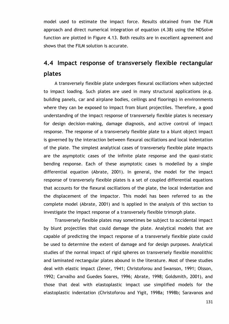
131

model used to estimate the impact force. Results obtained from the FILM

approach and direct numerical integration of equation (4.38) using the NDSolve

function are plotted in Figure 4.13. Both results are in excellent agreement and

shows that the FILM solution is accurate.

4.4 Impact response of transversely flexible rectangular

plates

A transversely flexible plate undergoes flexural oscillations when subjected

to impact loading. Such plates are used in many structural applications (e.g.

building panels, car and airplane bodies, ceilings and floorings) in environments

where they can be exposed to impact from blunt projectiles. Therefore, a good

understanding of the impact response of transversely flexible plates is necessary

for design decision-making, damage diagnosis, and active control of impact

response. The response of a transversely flexible plate to a blunt object impact

is governed by the interaction between flexural oscillations and local indentation

of the plate. The simplest analytical cases of transversely flexible plate impacts

are the asymptotic cases of the infinite plate response and the quasi-static

bending response. Each of these asymptotic cases is modelled by a single

differential equation (Abrate, 2001). In general, the model for the impact

response of transversely flexible plates is a set of coupled differential equations

that accounts for the flexural oscillations of the plate, the local indentation and

the displacement of the impactor. This model has been referred to as the

complete model (Abrate, 2001) and is applied in the analysis of this section to

investigate the impact response of a transversely flexible trimorph plate.

Transversely flexible plates may sometimes be subject to accidental impact

by blunt projectiles that could damage the plate. Analytical models that are

capable of predicting the impact response of a transversely flexible plate could

be used to determine the extent of damage and for design purposes. Analytical

studies of the normal impact of rigid spheres on transversely flexible monolithic

and laminated rectangular plates abound in the literature. Most of these studies

deal with elastic impact (Zener, 1941; Christoforou and Swanson, 1991; Olsson,

1992; Carvalho and Guedes Soares, 1996; Abrate, 1998; Goldsmith, 2001), and

those that deal with elastoplastic impact use simplified models for the

elastoplastic indentation (Christoforou and Yigit, 1998a; 1998b; Saravanos and

132

Christoforou, 2002; Zheng and Binienda, 2007) that may introduce significant

errors in the prediction of the impact response of the plate (Christoforou and

Yigit, 1998b). The use of well validated elastoplastic contact models in the

complete modelling approach is quite challenging computationally, but has the

advantage of producing more reliable results and of providing details of the

impact response that would not have been obtained otherwise.

In this section, a flexible laminated plate structure called a trimorph plate

is investigated analytically for low-velocity, large mass impact. Large mass

impact is investigated because the impact duration falls within a range

(milliseconds) that could allow for realistic impact control action using piezo-

actuation (Yigit and Christoforou, 2000). The analytical modelling of the

trimorph plate combined the flexural oscillation models of the trimorph plate

(see Section 2.6) with the new contact model (see Section 3.2) and the single

degree of freedom model for the impactor displacement. This combination

produces a set of 𝑝 + 1 coupled differential equations that must be solved

simultaneously; 𝑝 represents the number of participating harmonics (vibration

modes). During low to medium velocity impact the vibrations of the target are

small in comparison to the plate thickness so that additional nonlinearities

arising from large displacements (see Section 2.6) can be safely ignored. It is

also customary to neglect natural viscous damping because the impact response

is highly transient and does not allow sufficient time for natural viscous damping

effects to become significant. The modelling approach used in this study allows

for the use of various boundary conditions, though the present analysis has been

limited to simply-supported boundary conditions for mathematical convenience.

The reduced models for the impact response of a simply-supported transversely

flexible plate based on the complete model are given as:

𝑊 1 𝑚𝑛 + 1 − 𝛼 𝐾 𝑊1 𝑚𝑛 = 𝐹(𝑡) 𝛾 𝑚𝑛 (4.44𝑎)

𝑊 2 = −𝐹(𝑡)/𝑚𝑖 (4.44𝑏)

where 𝑊1 is the plate displacement; 𝑊2 is the displacement of the impactor; 𝐾

is the effective mechanical bending stiffness of the plate and is calculated as in

Section 2.6; 𝐷𝑖𝑗 are bending stiffness elements and can be calculated as in

Section 2.5; 𝑎 and 𝑏 are the planar dimensions of the plate; 𝛼 is a parameter to

alter the effective stiffness of the plate; 𝑚 and 𝑛 represent vibration mode

numbers; 𝑚𝑖 is the mass of the impactor; 𝐹(𝑡) = 𝐹 𝛿(𝑡) is the impact force

133

acting at the point of contact and is estimated from a static contact model; and

𝛿 = 𝑊2 −𝑊1 is the local indentation of the plate. The load coefficient 𝛾 is

defined by the distribution of the external excitation (see equation 2.43c). For a

point load at 𝑥0,𝑦0

𝛾 =4

𝜌𝑕𝑎𝑏Sin

𝑚𝜋𝑥0

𝑎 Sin

𝑛𝜋𝑦0

𝑏 (4.45𝑎)

For uniformly distributed load over a rectangular patch of width 𝑙1 and length 𝑙2

𝛾 =16

𝜌𝑕𝑚𝑛𝑐𝑑Sin

𝑚𝜋𝜆

𝑎 Sin

𝑛𝜋휂

𝑏 Sin

𝑚𝜋𝑙12𝑎

Sin 𝑛𝜋𝑙22𝑏

(4.45𝑏)

where 𝜌 is the plate density; 𝑕 is the total thickness of the plate; 𝜆 and 휂 are the

distances of the centre of the patch from the edges of the plate. The

rectangular patch covers the region defined by: 𝜆 − 𝑙1/2 < 𝑥 < 𝜆 + 𝑙1/2 and

휂 − 𝑙2/2 < 𝑦 < 휂 + 𝑙2/2. The load coefficients for other types of load distribution

can be found in the literature (Nosier et al, 1994; Reddy, 2004; Szilard, 2004).

Results presented in this section are obtained using equation (4.45a).

Equation (4.44a) was derived from the vibration models presented in

Section 2.6 by neglecting natural viscous damping and replacing the harmonic

excitation by a general excitation force. Equation (4.44a) is in vector form and

consists of 𝑚 + 1 (𝑛 + 1)/4 equations because 𝑚 and 𝑛 are odd for central

displacement of the plate. Equations (4.44a) and (4.44b) were solved, together

with the new contact model, using customised codes that automatically

generate the number of equations based on the specified values of 𝑚 and 𝑛, and

solves the equations simultaneously using the NDSolve function (see appendix

B.3). The contact model of Majeed et al (2012) was used for comparison because

of its simplicity. While this model underestimates the contact force during

substantial elastoplastic indentation of metals (see Figures 3.7 and 3.8), it was

nevertheless shown to produce similar estimates as the new contact model for

indentations in the range 0 < 𝛿 < 8𝛿𝑦 (see Figure 3.9). Since the impact events

investigated here have maximum indentations that fall within this range, using

the model of Majeed et al (2012) for the purpose of comparison is reasonable.

134

4.4.1 Validation of modelling and solution approach

To validate the combined modelling (complete model) and solution

(numerical integration using NDSolve function in Mathematica™) approach used

in the present analysis, a well-known impact problem first studied by Karas

(1939) and known as the ‘Karas problem’ is re-examined. This problem has been

studied by many others including Goldsmith (2001) and Abrate (1998) and can be

considered as a benchmark case. The impact event involves the elastic impact of

a simply-supported square steel plate struck by a steel ball. The material and

geometrical properties of the impact system were obtained from Abrate (1998)

as follows: density = 7806 [kg/m3], Young’s modulus = 206.8 [GPa] and Poisson’s

ratio = 0.3 [-]; Impactor diameter = 0.02 [m]; impact velocity = 1.0 [m/s]; Plate

dimensions = 0.2 × 0.2 × 0.008 [m3]. The impactor mass was calculated to be

0.0327 [kg]. Since the impact is elastic the Hertz contact model is used to

estimate the impact force, and the bending stiffness is calculated as 𝐾 =

𝐸𝑕2/12𝜌(1 − 𝜐2) 𝑚/𝑎 2 + 𝑛/𝑏 2 2 for a monolithic plate (Karas, 1939); where

𝐸, 𝜌, and 𝜐 are the Young’s modulus, density and Poisson ratio respectively.

The results obtained by Karas (1939), Abrate (1998) and the present

approach are compared in Figures 4.14a and 4.14b. Karas (1939) and Abrate

(1998) both used the complete modelling approach, but while the former solved

the reduced models using a small-increment time integration scheme the latter

employed the Newmark time integration scheme. The impactor – plate mass

ratio is 0.0131 and this means that the impact is a small mass impact (Olsson,

2000). Small mass impacts are dominated by highly dynamic flexural oscillations

and therefore, the solution to the reduced models of the complete modelling

approach requires that a good number of harmonics are considered to obtain

accurate results (Goldsmith, 2001). Karas (1939) used 70 harmonics while the

present solution was found to converge using 42 harmonics (i.e. m = 13 and n =

11). The results of all three methods are in good agreement. This shows that the

results obtained using the NDSolve function are reliable. Hence, the NDSolve

function has been used to solve the elastoplastic impact models of the trimorph

plate investigated in this study.

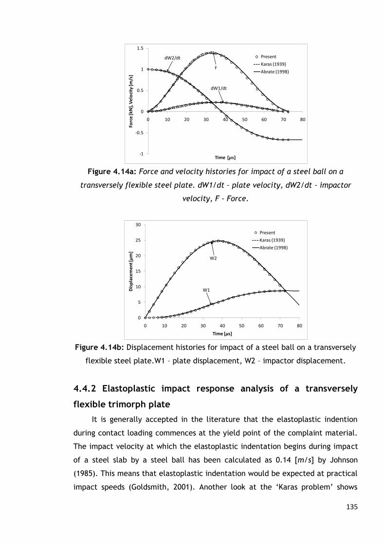
135

-1

-0.5

0

0.5

1

1.5

0 10 20 30 40 50 60 70 80

Forc

e [k

N],

Ve

loci

ty [m

/s]

Time [µs]

Present

Karas (1939)

Abrate (1998)

dW2/dt

F

dW1/dt

0

5

10

15

20

25

30

0 10 20 30 40 50 60 70 80

Dis

pla

cem

en

t [µ

m]

Time [µs]

Present

Karas (1939)

Abrate (1998)

W1

W2

Figure 4.14a: Force and velocity histories for impact of a steel ball on a

transversely flexible steel plate. dW1/dt – plate velocity, dW2/dt – impactor

velocity, F – Force.

Figure 4.14b: Displacement histories for impact of a steel ball on a transversely

flexible steel plate.W1 – plate displacement, W2 – impactor displacement.

4.4.2 Elastoplastic impact response analysis of a transversely

flexible trimorph plate

It is generally accepted in the literature that the elastoplastic indention

during contact loading commences at the yield point of the complaint material.

The impact velocity at which the elastoplastic indentation begins during impact

of a steel slab by a steel ball has been calculated as 0.14 [m/s] by Johnson

(1985). This means that elastoplastic indentation would be expected at practical

impact speeds (Goldsmith, 2001). Another look at the ‘Karas problem’ shows

136

that the maximum indentation during the impact loading is 20.36 [µm]. Karas did

not state the yield stress of the steel plate because it is not needed for elastic

impact analysis. Typical values of the yield stress for medium carbon steel range

from 245 [MPa] to 1740 [MPa] (Source: www.Matweb.com; Accessed: 13-10-

2014). The indentation at which elastoplastic indentation begins can be

determined from equation (3.2) (Stronge, 2000a; Majeed et al, 2012). For a yield

stress of 1740 [MPa] the indentation at yield was calculated as 15.75 [µm] using

equation (3.2) and this value is lower than the maximum indentation when the

impact is considered to be elastic. This means an impact velocity of 1.0 [m/s]

would give rise to elastoplastic indentation when the plate material is medium

carbon steel. In that case the Hertz contact model would not be ideal for

estimating the impact response. This section presents detailed investigations of

the elastoplastic impact response of a transversely flexible trimorph plate when

struck in the transverse direction by a rigid projectile with spherical contact

surface. First, the material properties of the trimorph plate are discussed and

then results of the elastoplastic impact response of the trimorph plate are

considered.

4.4.2.1 Material properties of a transversely flexible trimorph plate

In order to estimate the impact force using static indentation models, the

material properties (Young’s modulus, Poisson ratio and yield stress) of the

impactor and plate must be known. For the trimorph plate impact problem, the

impactor is considered to be made of a homogeneous isotropic material and the

material properties can be readily obtained from property tables e.g.

www.Matweb.com. However, the material properties of the trimorph plate in

the transverse direction (z-direction) cannot be obtained from property tables

because the plate consists of three different isotropic materials bonded

together. Ideally, experimental measurements of the material properties of the

trimorph plate would be available. In the absence of such experimental data the

properties can be determined from finite element simulations or approximate

analytical techniques.

An approximate analytical solution to the problem is the ‘strength of

materials’ approach (Khalili et al, 2007c). Khalili et al (2007c) used this

approach to determine the transverse properties of a rectangular sandwich plate

137

subjected to low-velocity impact. The sandwich plate was composed of two

symmetric composite laminate layers with a transversely flexible core. Two

different sandwich compositions were investigated. The first sandwich plate was

made of IM7/5260 composite face-sheets and a glass phenolic honeycomb core,

while the second plate was made of LTM45EL-CF0111 carbon fibre face-sheets

and high-density 110WF polymethacryimide foam core. In studying the response

of a functionally graded rectangular plate to low-velocity impact, Shariyat and

Farzan (2013) determined the transverse material properties of a plate made up

of a layer of zirconia on top and aluminium underneath using the strength of

materials approach. Since the plate was considered to be functionally graded

the volume fraction of each layer was determined from a power law that is

generally applied to functionally graded materials (Reddy, 2004; Shariyat and

Farzan, 2013). Shariyat and Jafari (2013) studied the impact response of a

functionally graded circular plate resting on an elastic foundation. The plate was

made of an alumina layer on top and an aluminium layer below. The transverse

properties of the plate were determined using strength of materials approach.

Larson and Palazotto (2009) estimated the transverse material properties of a

functionally graded rectangular plate made of a titanium boride (TiB) layer on

top and a Titanium (Ti) layer below using four different property estimation

methods, namely: the rule of mixtures method (strength of materials approach),

the self consistent method, the Mori-Tanaka spheres method and the Mori-

Tanaka needles method. All four methods were found to produce similar

estimates of the transverse properties of the TiB/Ti plate. A comparison with

published data showed that the rule of mixtures approach produced good

estimates of the transverse properties of the TiB/Ti plate. Furthermore, a

comparison was made of the maximum impact force determined from strain

gauge measurements and material property estimates from the four methods.

The comparison showed that the rule of mixtures approach produced similar

estimates of the maximum contact force to predictions using the other

approaches.

In this investigation, the strength of materials approach has been applied

to estimate the transverse material properties of the trimorph plate because of

its simplicity and ability to produce good estimates of the transverse material

properties for laminated plates made up of different materials. Khalili et al

(2007c) suggested that the strength of materials approach could be used under

138

plane stress conditions, quasi-static loading, and when the effect of the in-plane

material properties of the target on the transverse deformation, can be

neglected. These conditions apply to the impact of the trimorph plate, and

therefore, the strength of materials approach is considered to be suitable for

the present investigation.

The strength of materials approach can be used to estimate the Young’s

modulus, Poisson ratio, density and yield stress of the trimorph plate as shown.

𝐸𝑡 = 𝑕/ 𝑕1 𝐸1 + 𝑕2 𝐸2 + 𝑕3 𝐸3

𝑣𝑡 = 𝑣1𝑕1 + 𝑣2𝑕2 + 𝑣3𝑕3 /𝑕

𝜌𝑡 = 𝜌1𝑕1 + 𝜌2𝑕2 + 𝜌3𝑕3 /𝑕

𝑆𝑦𝑡 = 𝑕/ 𝑕1 𝑆𝑦1 + 𝑕2 𝑆𝑦2 + 𝑕3 𝑆𝑦3

(4.46)

where 𝑕 = 𝑕1 + 𝑕2 + 𝑕3 is the total thickness of the plate, the subscript, 𝑡,

represents the target which here is the plate; the subscripts 1, 2, and 3

represent the layers of the plate from bottom to top; 𝑕𝑘, 𝐸𝑘, 𝑣𝑘, 𝜌𝑘, and 𝑆𝑦𝑘 are

the thickness, Young’s modulus, Poisson’s ratio, density and yield stress of the

kth layer of the trimorph plate, respectively. The first three equations of

equations (4.46) have been used by Khalili et al (2007c), Shariyat and Farzan

(2013) and Shariyat and Jafari (2013). For the last equation in equations (4.46),

it is considered that because the yield point is the elastic limit then the

effective transverse yield stress of the trimorph plate can be determined in the

same way as the Young’s modulus. The assumption on the yield stress is not

based on theory or experimental observation, but at least it attempts to account

for the yield effect of all the materials of the trimorph plate.

4.4.2.2 Results and discussions on the elastoplastic impact response of

an Al/PVDF/PZT trimorph plate

A study of the elastoplastic impact response of a transversely flexible

trimorph plate with layers arranged as Al/PVDF/PZT from top to bottom was

carried out. The spherical surface of the impactor is in contact with the

aluminium layer. This layer arrangement of the trimorph plate has been used for

the impact studies because it has already been shown to exhibit the highest

mechanical bending stiffness (see Table 2.2). The material and geometrical

properties of the plate layers are shown in Table 4.5, and unless otherwise

stated, these properties are used in all the analyses that follow.

139

Table 4.5: Material and geometrical properties of the layers of the trimorph

plate

Material ν [-] E [GPa] ρ [kg/m3] Sy [MPa] h [mm]

Al 0.33 70 2700 320 3.0

PVDF 0.44 1.1 1770 50 1.0

PZT 0.3 64 7600 250 1.0

The other material and geometrical properties of the impact system are:

𝑎 = 100 [𝑚𝑚]; 𝑏 = 100 [𝑚𝑚]; 𝑚𝑖 = 1.0 [𝑘𝑔]; 𝑉0 = 0.30 [𝑚/𝑠]; 𝐸𝑖 = 210 [𝐺𝑃𝑎];

𝜈𝑖 = 0.30; 𝑅𝑖 = 10 [𝑚𝑚]; 𝛼 = 0. Impactor material: steel.

Effect of number of vibration modes used in the solution

The accuracy of the solution of the impact response of the Al/PVDF/PZT

plate depends on the number of participating modes used in the solution. The

impact force history was determined for different numbers of participating

modes as shown in Figure 4.15. The figure shows that nine participating modes

(i.e. 𝑚 = 𝑛 = 5) are sufficient to guarantee accurate results. This observation

was made previously by Khalili et al (2007a) who carried out a similar

convergence study for the elastic impact response of a SMA-composite hybrid

plate. The mass ratio of the impactor-trimorph plate system in Figure 4.15 is

5.72, which implies that the impact event is a large mass impact (Olsson, 2000).

Also, the convergence study carried out by Khalili et al (2007a) was for a large

mass impact. The impact response of a large mass impact is dominated by the

fundamental mode of vibration (Olsson, 2000; Abrate, 2001) and this explains

why the solution converges using just a few vibration modes. Hence, the results

presented and discussed in this section have been obtained using a nine mode

approximation. In Figure 4.15, the blue lines represent the elastic loading

response, the red lines represent the elastoplastic loading response, and the

black lines represent the response when unloading from an elastoplastic loading

stage. This colour definition has also been used in later figures.

140

0

0.1

0.2

0.3

0.4

0.5

0.6

0.7

0 0.5 1 1.5 2

Imp

act

fo

rce

[kN

]

Time [ms]

1 mode

9 modes

20 modes

0.5 1.0 1.5Time ms

0.05

0.10

0.15

Disp. mm

Figure 4.15: Effect of number of modes used in the solution of the impact

model on the accuracy of the results obtained for the Al/PVDF/PZT plate.

Figure 4.16: Displacement histories of Al/PVDF/PZT plate impacted by steel

impactor. Dotted line – impactor disp., short-dash line – plate disp., solid line –

indentation.

Figure 4.16 shows the displacements during the elastoplastic impact

response of the Al/PVDF/PZT plate. The displacement of the impactor is smooth

whereas there are oscillations in the displacement of the plate giving rise to

oscillations in the indentation. The response has a maximum indentation of

103.95 [μm], which occurs in the elastoplastic loading regime, and a permanent

141

0.5 1.0 1.5Time ms

0.2

0.1

0.1

0.2

0.3

Vel. ms

indentation of 21.16 [μm]. The maximum contact force is 573.95 [N] and the

impact duration is 1.88 [ms]. The loading ends when the velocity of the impactor

is zero and this occurs when the time is 0.94 [ms] (see Figure 4.17). The

indentation plot (see Figure 4.16) shows that the point of maximum indentation

(0.89 [ms], 103.95 [μm]) is different compared to the end point of the impact

loading (0.94 [ms], 99.7 [μm]), and this observation has also been reported

previously by Abrate (1998).

Figure 4.17: Velocity histories of Al/PVDF/PZT plate struck by steel impactor.

Dotted line – impactor velocity, short-dash line – plate velocity, solid line –

relative velocity.

Effect of contact model used to estimate the impact force

Figure 4.18 shows the impact force history for an initial impact velocity of

2.0 [m/s], and compares the results obtained when three different contact

models (newly proposed contact model, the contact model of Majeed et al

(2012) and the Hertz contact model) are used to estimate the impact force. The

force histories predicted by all three models are in good agreement,

demonstrating that the force history is not sensitive to the contact model used.

The insensitivity of the force history to the contact model arises because the

event is a large mass impact (Abrate, 1998; Chai and Zhu, 2011). For this reason,

some investigators (Khalili et al, 2007a; 2007b; Abrate 2001; Anderson, 2005) use

simplified contact models that do not account for elastoplastic indentation

effects to predict the impact response of plates subjected to large mass impact.

142

0

1

2

3

4

5

6

0 0.5 1 1.5 2

Imp

act

fo

rce

[kN

]

Time [ms]

Present

Hertz

Majeed et al (2012)

Whereas the use of such simplified contact models could significantly reduce the

computational effort involved and produce reliable estimates of the maximum

contact force and impact duration, they ignore the fact that elastoplastic

deformation may occur and therefore do not provide any information on the

elastoplastic response when it does occur.

As Figure 4.19 reveals, the indentation history predicted by the Hertz

contact model is different from that predicted by the elastoplastic contact

models. The elastoplastic contact models predict significant elastoplastic

deformation with a permanent indentation at the end of the impact. The new

contact model predicts a maximum indentation of 0.37 [mm] and a permanent

indentation of 59.8 [μm], the contact model of Majeed et al (2012) predicts 0.38

[mm] and 65.7 [μm] respectively, while the Hertz contact model predicts a

maximum indentation of 0.34 [mm] and no permanent indentation (see Figure

4.19). This shows that the contact model used for predicting the impact

response of a large mass impact can limit the information that can be obtained.

Details of an elastoplastic response, such as the permanent and maximum

indentation depth, are needed to develop and implement robust damage

mitigation strategies. This makes the choice of contact model used to study

large mass impact events an important consideration.

Figure 4.18: Force history of Al/PVDF/PZT plate struck by steel impactor with

initial impact speed of 2.0 [m/s].

143

0

0.05

0.1

0.15

0.2

0.25

0.3

0.35

0.4

0 0.5 1 1.5 2

Ind

en

tati

on

[mm

]

Time [ms]

Present

Hertz

Majeed et al (2012)

Figure 4.19: Indentation history of Al/PVDF/PZT plate struck by steel impactor

with initial impact speed of 2.0 [m/s].

Effect of transverse shear deformation

In Section 2.6.2 it was shown that transverse shear deformation affects the

displacement of a plate when the plate is moderately thick. The transverse

shear deformation effect was modelled using the FSDPT. The effect of

transverse shear deformation, on the impact response of a moderately thick

trimorph plate, was investigated by comparing the impact response of the

Al/PVDF/PZT plate obtained using both the CLPT and FSDPT. A thickness of 8.0

[mm] was used for the aluminium layer, making a total plate thickness of 10.0

[mm]. Since the planar dimension of the trimorph plate is 100 × 100 [mm2], the

thickness to length ratio is 1/10, satisfying the geometrical condition for

moderately thick plates. The impact response, based on the two plate theories

(CLPT and FSDPT) are shown in Figures 4.20 a – c. The results show that shear

deformation affects the plate displacement (Figure 4.20a) but has negligible

effect on the indentation and impact force histories (Figures 4.20b, c). This is

because shear deformation effects become more pronounced at higher vibration

modes, which have very little effect on the response of a large mass impact, as

considered here. The present investigation is limited to the indentation and

impact force of large mass impact events and therefore, all other results have

been obtained using the CLPT.

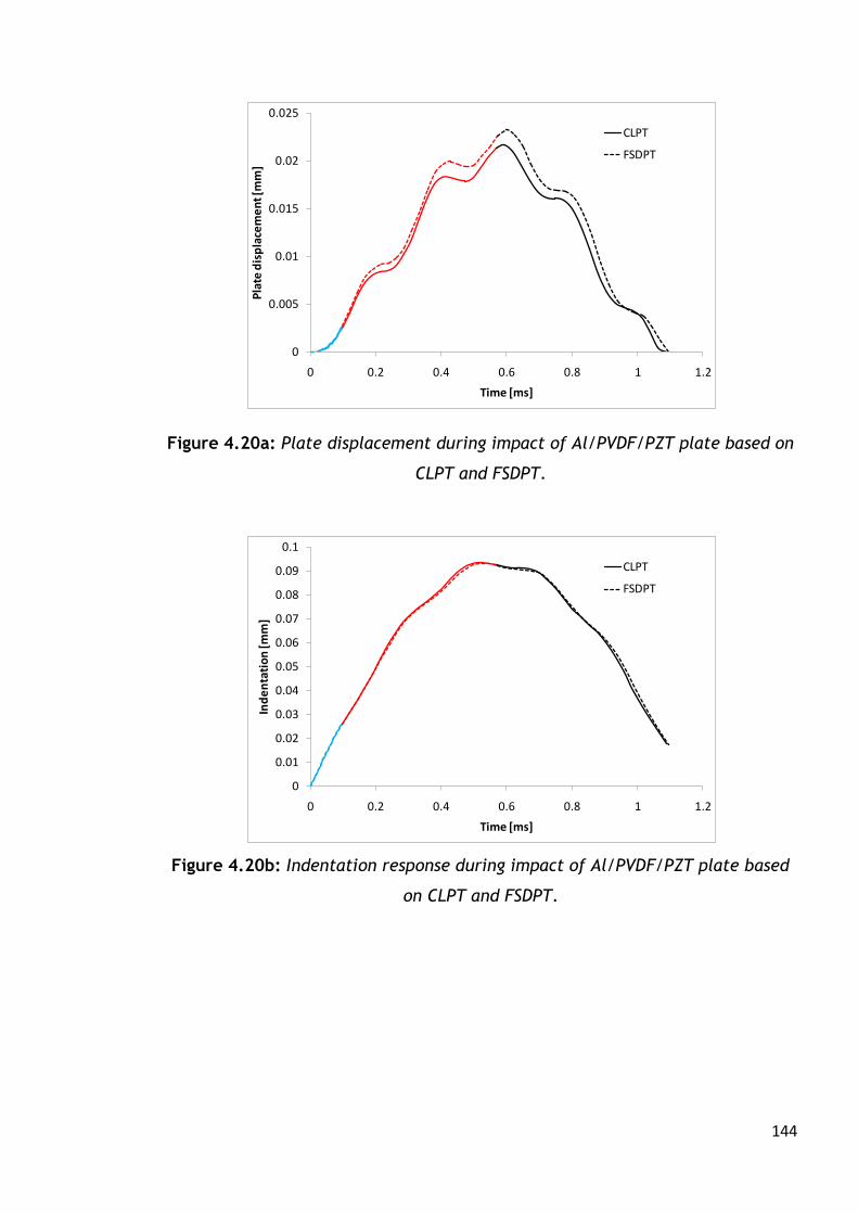
144

0

0.01

0.02

0.03

0.04

0.05

0.06

0.07

0.08

0.09

0.1

0 0.2 0.4 0.6 0.8 1 1.2

Ind

en

tati

on

[mm

]

Time [ms]

CLPT

FSDPT

0

0.005

0.01

0.015

0.02

0.025

0 0.2 0.4 0.6 0.8 1 1.2

Pla

te d

isp

lace

me

nt [

mm

]

Time [ms]

CLPT

FSDPT

Figure 4.20a: Plate displacement during impact of Al/PVDF/PZT plate based on

CLPT and FSDPT.

Figure 4.20b: Indentation response during impact of Al/PVDF/PZT plate based

on CLPT and FSDPT.

145

0

0.2

0.4

0.6

0.8

1

1.2

0 0.2 0.4 0.6 0.8 1 1.2

Imp

act

fo

rce

[kN

]

Time [ms]

CLPT

FSDPT

Figure 4.20c: Force response during impact of Al/PVDF/PZT plate based on

CLPT and FSDPT.

For better understanding of the impact response of the Al/PVDF/PZT plate,

the influence of critical impact and geometrical parameters on the impact

response is investigated. The effects of impactor mass, impactor size, initial

impact velocity and the thickness and aspect ratio of the plate, on the impact

response were examined and the results are shown in Figures 4.21 to 4.25.

Effect of impactor mass

To study the effect of the impactor mass on the impact response of the

Al/PVDF/PZT plate, the impactor mass was varied without changing the radius of

the impactor in contact with the plate. In practice this can be achieved by using

impactors with hemispherical contact end. A comparison of the contact force

histories for different impactor masses is shown in Figure 4.21. It is observed

that a higher impactor mass results in a higher maximum impact force, longer

impact duration and more oscillations in the impact force. Also, the permanent

indentation increases with increasing impactor mass. Note that comparison of

the permanent indentation is performed by visual inspection of the plots for the

impact force histories; the larger the vertical height of the elastoplastic

response (red lines), the larger the permanent indentation and vice versa. This

observation is found to be consistent with permanent indentation results of the

indentation history plots. The latter are not shown because they are not

necessary for the discussions in this investigation.

146

0

0.2

0.4

0.6

0.8

1

1.2

1.4

1.6

0 0.5 1 1.5 2 2.5 3 3.5 4

Imp

act

fo

rce

[kN

]

Time [ms]

m = 0.5 kg

m = 1.0 kg

m = 2.0 kg

m = 5.0 kg

0

0.1

0.2

0.3

0.4

0.5

0.6

0.7

0 0.5 1 1.5 2

Imp

act

fo

rce

[kN

]

Time [ms]

Ri = 5 mm

Ri = 10 mm

Ri = 15 mm

Figure 4.21: Effect of impactor mass on the impact response of Al/PVDF/PZT

plate.

Figure 4.22: Effect of impactor size on the impact response of Al/PVDF/PZT

plate.

Effect of impactor size

The impactor size is represented by the radius of the impactor in contact

with the target. The radius of the impactor was varied without changing the

impactor mass. Again, this can be achieved in practice by using impactors with

hemispherical contact end. The effect of the impactor size is simulated using

the impact force histories, as shown in Figure 4.22. An increase in the impactor

size results in a higher maximum impact force, shorter impact duration, and

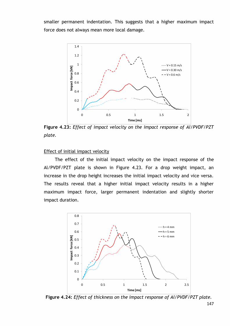
147

0

0.1

0.2

0.3

0.4

0.5

0.6

0.7

0.8

0 0.5 1 1.5 2 2.5

Imp

act

fo

rce

[kN

]

Time [ms]

h = 4 mm

h = 5 mm

h = 6 mm

0

0.2

0.4

0.6

0.8

1

1.2

1.4

0 0.5 1 1.5 2

Imp

act

fo

rce

[kN

]

Time [ms]

V = 0.15 m/s

V = 0.30 m/s

V = 0.6 m/s

smaller permanent indentation. This suggests that a higher maximum impact

force does not always mean more local damage.

Figure 4.23: Effect of impact velocity on the impact response of Al/PVDF/PZT

plate.

Effect of initial impact velocity

The effect of the initial impact velocity on the impact response of the

Al/PVDF/PZT plate is shown in Figure 4.23. For a drop weight impact, an

increase in the drop height increases the initial impact velocity and vice versa.

The results reveal that a higher initial impact velocity results in a higher

maximum impact force, larger permanent indentation and slightly shorter

impact duration.

Figure 4.24: Effect of thickness on the impact response of Al/PVDF/PZT plate.

148

0

0.1

0.2

0.3

0.4

0.5

0.6

0.7

0 0.5 1 1.5 2 2.5

Imp

act

fo

rce

[kN

]

Time [ms]

b/a = 0.5

b/a = 1

b/a = 5

b/a = 10

Effect of plate thickness

The total thickness of the Al/PVDF/PZT plate was varied by changing the

thickness of the Al layer. Hence, the thicknesses of the Al layer used in the

simulations are 2 [mm], 3 [mm] and 4 [mm]. The thickness effect is shown in

Figure 4.24. The figure shows that increasing the total thickness of the plate

results in a shorter impact duration and higher maximum impact force. Also, the

permanent indentation increases due to more a localised response.

Figure 4.25: Effect of aspect ratio on the impact response of Al/PVDF/PZT

plate.

Effect of plate aspect ratio

The effect of the aspect ratio of the plate (i.e. the ratio of the planar

dimensions) on the impact response was considered by simulating the impact

response for four different aspect ratios as shown in Figure 4.25. An ideal aspect

ratio for comparison is 1. Figure 4.25 shows that for an aspect ratio of 0.5, the

response becomes more localised and it is characterised by a higher maximum

impact force, shorter impact duration, more post-yield deformation and less

oscillations. For an aspect ratio of 5, the maximum contact force is lower and

the impact duration is longer. This is because the plate with an aspect ratio of 5

is more flexible than that with an aspect ratio of 1. However, an aspect ratio of

10 shows a slightly more localised response in comparison to an aspect ratio of

1. This shows that the flexibility of a plate during impact cannot be fully

understood by considering the aspect ratio alone.

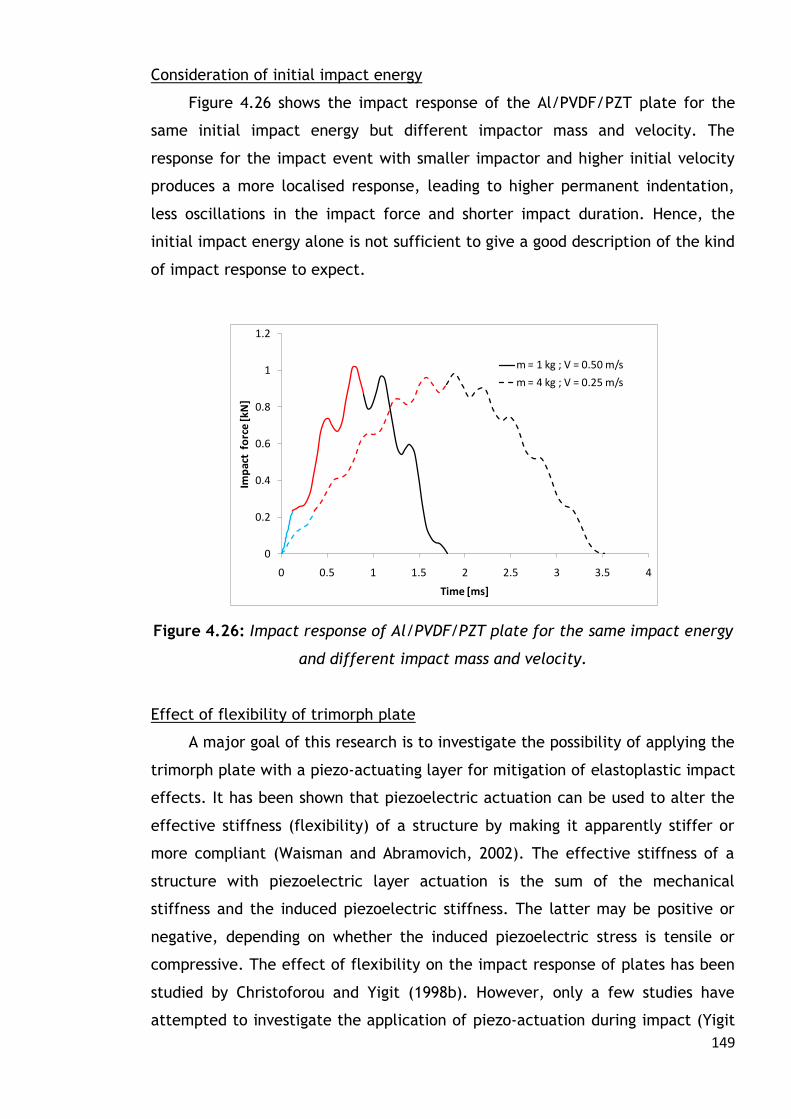
149

0

0.2

0.4

0.6

0.8

1

1.2

0 0.5 1 1.5 2 2.5 3 3.5 4

Imp

act

fo

rce

[kN

]

Time [ms]

m = 1 kg ; V = 0.50 m/s

m = 4 kg ; V = 0.25 m/s

Consideration of initial impact energy

Figure 4.26 shows the impact response of the Al/PVDF/PZT plate for the

same initial impact energy but different impactor mass and velocity. The

response for the impact event with smaller impactor and higher initial velocity

produces a more localised response, leading to higher permanent indentation,

less oscillations in the impact force and shorter impact duration. Hence, the

initial impact energy alone is not sufficient to give a good description of the kind

of impact response to expect.

Figure 4.26: Impact response of Al/PVDF/PZT plate for the same impact energy

and different impact mass and velocity.

Effect of flexibility of trimorph plate

A major goal of this research is to investigate the possibility of applying the

trimorph plate with a piezo-actuating layer for mitigation of elastoplastic impact

effects. It has been shown that piezoelectric actuation can be used to alter the

effective stiffness (flexibility) of a structure by making it apparently stiffer or

more compliant (Waisman and Abramovich, 2002). The effective stiffness of a

structure with piezoelectric layer actuation is the sum of the mechanical

stiffness and the induced piezoelectric stiffness. The latter may be positive or

negative, depending on whether the induced piezoelectric stress is tensile or

compressive. The effect of flexibility on the impact response of plates has been

studied by Christoforou and Yigit (1998b). However, only a few studies have

attempted to investigate the application of piezo-actuation during impact (Yigit

150

0

0.05

0.1

0.15

0.2

0.25

0.3

0 0.5 1 1.5 2 2.5 3 3.5

Imp

act

fo

rce

[kN

]

Time [ms]

30% decrease

No change

30% increase

and Christoforou, 2000; Saravanos and Christoforou, 2002). A parametric study

was carried out to demonstrate that the flexibility of a trimorph plate could be

exploited to mitigate impact effects. To achieve this, a parameter, 𝛼, used to

alter the effective stiffness of the trimorph plate without changing the

dimensions or material properties of the plate (as would be expected during

piezo-actuation – see Section 5.4.1) was introduced as shown in equation

(4.44a). 𝛼 represents the percentage change in the effective stiffness of the

plate. When 𝛼 < 0, the plate is apparently less flexible and when 𝛼 > 0, the

plate is apparently more flexible. The normal case is represented by 𝛼 = 0 when

the effective stiffness is determined by the mechanical stiffness only.

Figure 4.27: Influence of apparent flexibility on the impact response of

Al/PVDF/PZT plate.

Figure 4.27 shows the effect of 𝛼 on the impact response of the

Al/PVDF/PZT plate. In this figure, the mass of the impactor is 2.0 [kg] and the

impact velocity is 0.1 [m/s]. Three cases are considered for illustration purposes

i.e. 𝛼 = 0, 𝛼 = −0.3, and 𝛼 = 0.3. The reference point is taken when the

effective stiffness is equal to the mechanical stiffness i.e. 𝛼 = 0. For 𝛼 = 0, the

maximum impact force is 246.15 [N], the impact duration is 2.73 [ms] and the

permanent indentation is 3.36 [μm]. When 𝛼 = −0.3, the effective stiffness is

30% higher than normal (𝛼 = 0) and the impact response, which is more

localised, is characterised by a higher maximum impact force (263.45 [N]),

151

shorter impact duration (2.60 [ms]) and larger permanent indentation (5.10

[μm]). For 𝛼 = 0.3, the effective stiffness is 30% lower than normal and the

response has become purely elastic with no permanent indentation. The

maximum impact force is about 4.0% lower than for 𝛼 = 0 and the impact

duration is longer (3.02 [ms]). The implication is that an impact, which should

ordinarily result in a permanent indentation, can be converted to one with no

permanent indentation. This result is significant because it demonstrates that

alteration of the effective stiffness of the plate could be exploited to either

reduce or completely eliminate elastoplastic impact effects. In general, an

increased flexibility through reduction of the effective stiffness of the plate

would result in reduced local effects and increased global effects, and vice

versa. The alteration of the effective stiffness of a plate with piezoactuator

layer(s) can be achieved through the piezo-actuation effect (Waisman and

Abramovich, 2002); this notion is investigated further in the next chapter.


This chapter presents a detailed treatment of the impact response of

rectangular plates. The impact response of two kinds of plate was studied,

namely: transversely inflexible (very thick) and transversely flexible (thin to

moderately thick) plates. For the former, the response was predicted using half-

space assumptions and the investigations showed that the contact model used to

predict the impact force was an important factor on the resulting predictions. It

was also observed that the amount of impact energy dissipated as non-

recoverable plastic deformation was a function of the initial impact velocity, i.e.

a high initial velocity results in more non-recoverable plastic deformation.

An analytical solution algorithm called the FILM was developed to solve the

nonlinear models for the elastoplastic impact response of transversely inflexible

plates. The solution algorithm was shown to produce results which matched

those obtained by direct numerical integration of the nonlinear models using the

NDSolve function in Mathematica™. The implications of applying the FILM to

solve the nonlinear impact models for a transversely flexible plate were

discussed, and it was suggested that the FILM could be used to solve small mass

impact problems where there are no oscillations in the impact force. An example

of a small mass impact event with non-oscillating impact force is the infinite

152

plate impact, and the FILM was successfully used to determine the impact

response of an infinite plate case study. The strengths of the FILM approach are

its simplicity, inherent stability, fast-convergence rate and the fact that it could

be checked manually. However, when it is applied to solve the nonlinear models

of a transversely flexible plate it becomes semi-analytical, because the time at

the boundaries of each discretisation must be determined numerically. A

computer implementation is then required and the number of discretisations

needed to obtain accurate results is more compared to the case of transversely

inflexible plates.

The vibration models formulated in Chapter two and the new contact

model developed in Chapter three were combined in Section 4.4 of this chapter

using the complete modelling approach, to investigate the impact response of a

transversely flexible trimorph plate. The investigations show that the contact

model used to predict the impact force of a large mass impact event can

significantly affect the resulting predictions, and also limit detailed description

of the impact response. Transverse shear deformation was found to have no

significant effect on the indentation and impact force histories of a moderately

thick trimorph plate subjected to large mass impact. Critical impact and

geometrical parameters such as impactor mass, impactor velocity, impactor

size, plate thickness and plate aspect ratio were shown to influence the impact

response of the trimorph plate. Finally, a parametric study was carried out to

show that elastoplastic impact effects could be reduced or eliminated by

altering the effective stiffness of the plate; an observation that could be

exploited for active impact control. Control of the effective stiffness is

practically realisable using piezoactuators and further investigations of this

notion are discussed in Chapter five.

153

CHAPTER FIVE

MITIGATION OF ELASTOPLATIC IMPACT EFFECTS USING PIEZOACTUATORS

Chapter summary

Low-velocity impact of transversely flexible structures by rigid blunt

objects could result in damage of the structure. Studies on the mitigation of the

impact damage effects are mostly limited to passive mitigation strategies such

as structural fortification using materials with higher stiffness and better impact

energy absorption using sandwich construction with foam core. Relatively little

has been done in the area of active mitigation of low-velocity impact damage.

This chapter investigates the active mitigation of low-velocity impact damage by

means of induced pre-stress. The investigations were carried out analytically

using a novel nonlinear elastoplastic contact model (see Section 3.2) in the

complete modelling approach (see Section 4.4) to account for the localised

response of the plate considered. A linear piezoelectric theory was incorporated

into the impact model to account for induced strain actuation. The investigation

focuses on the effect of an induced pre-stress, produced by piezoelectric

actuation, on the impact response of a rectangular plate incorporating PZT

layers, and on how this effect can be utilised for active mitigation of

elastoplastic impact effects. The chapter concludes with a discussion of the

possible technological issues involved with practical implementation of induced

pre-stress as an active mitigation strategy against elastoplastic impact effects.

5.1 Review of impact damage of transversely flexible

plates

The impact of thin flexible plates by rigid blunt object normally results in

very high localised stresses that can damage the plate (Abrate, 1998).

Therefore, impact damage of flexible structures is an active area of theoretical,

numerical and experimental research. Understanding of impact damage of thin

plates is still evolving because it is a very complex and transient (micro- to

milliseconds) phenomenon involving many variables (material properties of the

plate and impactor, impactor shape and mass, relative impact speed of the plate

154

and impactor, geometry of the plate, and boundary conditions of the plate) and

different failure mechanisms. For thin monolithic metallic plates impact damage

occurs in the form of localised plastic deformation and/or perforation

(Goldsmith, 2001). During low- to medium-velocity impact on a thin monolithic

metallic plate, plastic deformation may occur without perforation, but the

plastic deformation can lead to a significant change of the plate stiffness,

relative to its original design value. The damage mechanism of thin monolithic

metallic plates during high-velocity impact involves both plastic deformation and

perforation. With thin laminated plates, impact damage may involve both

permanent deformation and/or delamination. Delamination is potentially

dangerous because even though it may be initiated at a high load compared to

the load required to initiate local permanent deformation, the delamination

damage propagates at a much lower load once initiated. In composite laminates,

delamination is caused by the global effect of the impact (Yigit and

Christoforou, 2000), whereas the local effect of the impact produces a

permanent deformation that is due to both plastic deformation of the matrix

and damage of the fibres, i.e. fibre breaking, kinking, and/or micro-buckling.

The local permanent deformation can be estimated using static contact models

that account for post-yield effects (Yigit and Christoforou, 1994).

Olsson (2001) formulated analytical models for the prediction of impact

damage initiation and growth during large mass impact. The models were

developed based on quasi-static bending assumption and the local indentation

was estimated using the Hertz contact model. The study revealed that the

critical load for delamination was generally insensitive to both the geometry and

boundary conditions, when the effects of membrane stretching are neglected.

The analytical model was validated by comparing analytical predictions with

experimental results. Olsson (2003) studied the delamination onset of laminated

composite plates during small mass impact. The expression for the peak impact

load was derived based on the Hertz contact model and from the closed-form

solutions of three asymptotic impact cases namely: (i) fully immobile plate

response, (ii) fully mobile plate with only bending response and (iii) fully mobile

plate with only transverse shearing response. The predicted peak load obtained

using the analytical formulation compared well with previously published

experimental results. The expression for the peak impact load was then used to

determine the threshold impact velocity required to initiate delamination.

155

Olsson et al (2006) derived closed-form solutions to determine the

delamination threshold load and velocity for small mass impact upon flexible

plates. The closed-form solutions were derived based on a modified form of the

Hertz contact model that accounts for thickness effect. The results of the

closed-form solution were shown to be in good agreement with selected finite

element results and previously published experimental data. Zheng and Binienda

(2007) studied the effect of permanent indentation on the delamination

threshold of composite plates subjected to small mass impact. A linearised

elastoplastic contact model was used to derive a closed-form solution for the

peak contact force. The threshold impact velocity to initiate delamination was

determined using the peak contact force and a quasi-static delamination

threshold load criterion. The study revealed that the peak force predicted, when

the impact force is estimated using the elastic Hertz contact model, is

significantly higher than that predicted when an elastoplastic contact model is

used to estimate the impact force. It was concluded that using the Hertz contact

model to estimate the impact force could lead to significant errors in the

estimation of the delamination threshold.

As explained earlier delamination in a composite laminate is caused by the

global effect of the impact. The local effect of the impact may lead to

permanent indentation which is another type of impact damage. Permanent

indentation is produced as a result of elastoplastic indentation during impact

loading. Contact models for elastoplastic indentation have been developed for

composite laminates (Sun and Yang, 1980; Yigit and Christoforou, 1994; Majeed

et al, 2012) and metallic targets (Stronge, 2000a; Brake, 2012; and the new

contact model presented in Section 3.2) and can be used to estimate the

permanent indentation. Furthermore, elastoplastic contact models give a more

accurate prediction of the impact response compared to the Hertz contact

model (Yigit and Christoforou, 1994; Majeed et al, 2012). Since the size of the

permanent indentation and the initiation of delamination are dependent on the

maximum impact force it is important to predict the maximum impact force

accurately, hence, the need to use elastoplastic contact models for impact

damage analysis.

The severity and type of damage (local or global) during impact of a

laminated plate depends on the impact force. The implication is that impact

damage effects can be mitigated by controlling the impact force. Increasing the

156

shock effect of the impact force leads to greater permanent deformation (local

damage) and less delamination (global damage) and vice versa (Yigit and

Christoforou, 2000). Since the impact response of a transversely flexible plate is

determined by interactions between the plate vibration and the impactor

displacement, a change in the vibration response of the plate inevitably leads to

a change in the impact response. Vibration control of a transversely flexible

plate can be achieved via induced strains produced by the actuation of bonded

PZT layers (Mitchell and Reddy, 1995; Liew et al, 2004). Hence, the impact force

can be controlled by the application of induced strains produced by the

actuation of bonded PZT-layers. In this chapter a strategy is proposed for the

mitigation of elastoplastic impact effects i.e. plastic deformation and damage.

The strategy is based on the use of induced-strain effect of bonded PZT layers to

control the impact force, and consequently the impact damage. An elastoplastic

contact model is applied in the formulation of the impact models to give a more

accurate estimate of the impact damage.

5.2 Impact damage mitigation

Impact damage of flexible structures due to low-velocity impact by rigid

blunt objects can be very severe and potentially dangerous. For instance the

impact of a freely flying runway debris on an aeroplane body can cause severe

localised damaged. Damage mitigation in this case should address the reduction

of damage effects on the structure since the debris is considered to be

sacrificial. In a situation where an accidental impact occurs between a

pedestrian and a car body, the car body becomes sacrificial in relation to the

pedestrian. Hence, damage mitigation in this case should address reduced shock

transfer to the pedestrian and this may be achieved by reducing the local effect

of the impact. Several studies have been carried out to investigate novel

strategies for mitigating impact damage effects. This section discusses some of

the passive and active strategies that have been investigated in previous studies.

5.2.1 Passive mitigation of impact damage

Mitigation of impact damage is generally considered under two sub-areas

namely: impact damage resistance and impact damage tolerance. The former is

concerned with resistance to damage formation and propagation while the later

157

is concerned with the ability of the impacted structure to safely perform its

intended function within an allowable damage size (Olsson, 2001; Emile and

Matthew, 2003). Impact damage mitigation strategies may improve either or

both. Impact damage resistance is normally achieved through structural

stiffening while impact damage tolerance is achieved using more resilient

materials or structural designs that are capable of absorbing most of the impact

energy in a way that minimises the damage size and retains structural integrity.

A lot has been done in the area of passive mitigation of impact damage. Some of

the passive mitigation strategies that have been applied to laminated composite

structures include fibre toughening, matrix toughening, interface toughening,

introduction of through-the-thickness reinforcement, selective interlayering and

use of hybrid composites (Angioni et al, 2011). Emile and Matthew (2003)

discussed various passive mitigation strategies for the development of impact

damage tolerant composites for aerospace structures. The passive mitigation

strategies discussed were essentially novel material design concepts that

included stitching, Z-pinning and 3-D composites. The authors concluded that

the best material design concepts for impact damage resistance are planar

woven and non-crimp fabric composites, while Z-pinned composites were

recommended for impact damage tolerance. It was also stated that 3-D

composites show considerable promise for impact tolerant material design. The

potential of 3-D composites as impact tolerant materials have also been

discussed by Mouritz et al (1999) and Kamiya et al (2000). A more recent study

(Mouritz and Cox, 2010) revealed that up to 20% increase in mechanical

properties can be achieved with 3-D composites compared to their equivalent 2-

D composites.

Shape memory alloys (SMAs) have being used for passive mitigation of

impact damage although they belong to the category of smart materials. In their

passive state SMAs can absorb significant levels of impact energy through plastic

deformation and stress-induced phase transformation, i.e. changing from an

austenitic to martensitic phase (Angioni et al, 2011). Lau et al (2004) studied the

low-velocity impact response of glass-epoxy composite plates fitted with

integrated stitching in the form of SMA wires. The stitched SMA wires helped to

improve the through-the-thickness reinforcement of the glass-epoxy composite

plate. Experimental and theoretical results revealed that the tensile strength of

the SMA stitched composite plate was increased and the number of impact-

158

induced translaminar cracks was reduced compared to the unstitched composite

plate. Analytical studies conducted by Khalili et al (2007a; 2007b) showed that

SMA wires embedded within a thin composite plate could significantly improve

the damage resistance of the composite plate to low-velocity impact. The

volume fraction, orientation and through-the-thickness location of the SMA wires

were all found to influence the impact damage of the plate. More on the passive

impact damage resistance and damage suppression using hybrid composites with

embedded SMA wires, can be found in Angioni et al (2011).

5.2.2 Active mitigation of impact damage

The literature on active mitigation of impact damage of flexible structures

when impacted by rigid blunt objects is limited (Yigit and Christoforou, 2000).

This can be attributed to the fact that active mitigation of impact damage is

challenging due to the complex and highly transient nature of the problem. Many

impact events typically occur in a time frame of micro- to milliseconds and may

not allow sufficient time for any meaningful control action to be taken during

the impact. Furthermore, the uncertainties in estimating the impactor

parameters (mass, velocity and size) make it difficult to determine the

appropriate level of active mitigation (Yigit and Christoforou, 2000).

Nevertheless, the active mitigation of impact damage using embedded SMA wires

has been investigated (Khalili et al, 2007d; Angioni et al, 2011) and a good

review of investigations in this area can be found in Angioni et al (2011). Khalili

et al (2007d) studied the effect of active stiffening in relation to the low-

velocity impact response of a composite plate with embedded SMA wires. The

stiffness of the hybrid composite plate incorporating SMA wires was divided into

two groups, namely: essential and acquired stiffness. The former is the stiffness

of the manufactured hybrid composite plate without any activation, while the

latter is the extra stiffness induced in the manufactured hybrid composite plate

following activation. The sum of the essential and acquired stiffnesses gives the

total stiffness of the hybrid composite plate when the active elements (SMA

wires in this case) are actuated. The results of the study by Khalili et al (2007d)

showed that the interactive effect between the essential stiffness and the

acquired stiffness can improve the impact damage resistance of the SMA hybrid

159

composite plate, compared to a similar hybrid composite plate with embedded

steel wires.

The smart stiffening procedure proposed by Khalili et al (2007d) is

conceptually reasonable but impractical with SMA actuators because of the

relatively slow response time of SMA wire; typically 3 – 4 seconds (Thompson and

Loughlan, 1995). An impact event would have finished before actuation of the

SMA wires could be realised. Therefore, actuators that can operate within

realistic impact times are more suitable candidates for active impact mitigation.

Piezoactuators are the fastest known actuators, having a response time of a few

milliseconds (Thompson and Loughlan, 1995; Yigit and Christoforou, 2000). As

observed from the results presented in Section 4.4.2.2 and previous studies

(Anderson, 2005; Olsson, 2002; Yigit and Christoforou, 2000; Saravanos and

Christoforou, 2002; Khalili et al, 2007a; 2007b) large mass impact events usually

have an impact duration of a few milliseconds. Hence, piezoactuators can be

used for active mitigation of large mass impact damage. On the other hand,

small to medium mass impact events normally have impact durations in the

range of microseconds and therefore only the post-impact induced damage

effects may be actively mitigated in such cases (Yigit and Christoforou, 2000).

Yigit and Christoforou (2000) proposed a linear quadratic regulator (LQR)

controller for active impact control and showed that the energy transferred to

the structure can be reduced by active control of the panel stiffness. The

technique was used to create a more localised impact response, thereby

reducing the vibration energy absorbed by the structure. Saravanos and

Christoforou (2002) studied the impact response of adaptive piezoelectric

laminated plates. Control of the impact response of the piezoelectric laminated

plate was implemented using state feedback and output feedback controllers.

The former was based on LQR controllers while the latter was based on the

signals produced by piezoelectric sensors. The study demonstrated that

considerable reductions in the impact force of laminated plates can be achieved

by active plate bending or damping induced by piezoelectric actuators.

However, the main issues with the practical implementation of the controllers

used in that study were:

a) The state feedback controllers require prior knowledge of all the state

variables (impactor and plate displacements and velocities). This

160

information may be difficult to estimate in real time (Yigit and Christoforou,

2000).

b) The sensory feedback controllers require sufficient time in order to provide

feedback signals for use by the actuators. Given that the maximum impact

force generally occurs during the impact loading which is usually within a

time of about half the impact duration, the maximum or critical impact

effects may have occurred before the sensor-actuator feedback loop is

complete.

A notable limitation of the study by Saravanos and Christoforou (2002) is that the

impact models were formulated based on a linearised elastoplastic contact law

that takes no account of permanent indentation effects. In the present

investigation, an elastoplastic contact model that accounts for permanent

indentation effects has been used. Also, the impact damage mitigation strategy

proposed here is based on the concept of pre-stressing induced by piezo-

actuation; this idea is explored in Section 5.4.

5.3 Piezoelectric actuation effect

Piezoelectric effect is a physical phenomenon exhibited by certain

crystalline materials whereby these materials generate surface electric charges

when an external stress is applied (Preumont, 2011). Examples of materials that

exhibit this behaviour are Rochelle salt, quartz, tourmaline and lead zirconate

titanate (PZT). This effect was discovered more than a century ago by the Curie

brothers. The production of surface electricity due to an externally applied

stress is known as the direct piezoelectric effect and is normally applied for

sensing. The converse piezoelectric effect is also possible and involves the

generation of induced strain in the material upon application of an electrical

voltage. The converse effect is applied in actuators to generate precisely

controllable induced strains (or stresses).

In their natural state piezoceramics do not exhibit any piezoelectricity.

Natural piezoceramics contain crystals that have no centre of symmetry and the

electric dipoles are randomly oriented with a net macroscopic dipole of zero.

This state of natural piezoceramics occurs below a critical temperature called

the Curie temperature. Piezoelectric effects are imparted to piezoceramic

through a process known as poling. During poling a high direct current electric

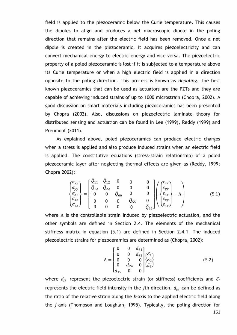
161

field is applied to the piezoceramic below the Curie temperature. This causes

the dipoles to align and produces a net macroscopic dipole in the poling

direction that remains after the electric field has been removed. Once a net

dipole is created in the piezoceramic, it acquires piezoelectricity and can

convert mechanical energy to electric energy and vice versa. The piezoelectric

property of a poled piezoceramic is lost if it is subjected to a temperature above

its Curie temperature or when a high electric field is applied in a direction

opposite to the poling direction. This process is known as depoling. The best

known piezoceramics that can be used as actuators are the PZTs and they are

capable of achieving induced strains of up to 1000 microstrain (Chopra, 2002). A

good discussion on smart materials including piezoceramics has been presented

by Chopra (2002). Also, discussions on piezoelectric laminate theory for

distributed sensing and actuation can be found in Lee (1999), Reddy (1999) and

Preumont (2011).

As explained above, poled piezoceramics can produce electric charges

when a stress is applied and also produce induced strains when an electric field

is applied. The constitutive equations (stress-strain relationship) of a poled

piezoceramic layer after neglecting thermal effects are given as (Reddy, 1999;

Chopra 2002):

𝜍𝑥𝑥𝜍𝑦𝑦𝜍𝑥𝑦𝜍𝑥𝑧𝜍𝑦𝑧

=

𝑄 11 𝑄 12 0

𝑄 12 𝑄 22 0

0 0 𝑄 66

0 0 0 0 0 0

0 0 0 0 0 0

𝑄 55 0

0 𝑄 44

휀𝑥𝑥휀𝑦𝑦휀𝑥𝑦휀𝑥𝑦휀𝑥𝑦

− Λ

(5.1)

where Λ is the controllable strain induced by piezoelectric actuation, and the

other symbols are defined in Section 2.4. The elements of the mechanical

stiffness matrix in equation (5.1) are defined in Section 2.4.1. The induced

piezoelectric strains for piezoceramics are determined as (Chopra, 2002):

Λ =

0 0 𝑑31

0 0 𝑑32

0 0 00 𝑑24 0 𝑑15 0 0

ℰ1

ℰ2

ℰ3

(5.2)

where 𝑑𝑗𝑘 represent the piezoelectric strain (or stiffness) coefficients and ℰ𝑗

represents the electric field intensity in the jth direction. 𝑑𝑗𝑘 can be defined as

the ratio of the relative strain along the k-axis to the applied electric field along

the j-axis (Thompson and Loughlan, 1995). Typically, the poling direction for

162

piezoceramics is the 3-direction (see Figure 5.1). Hence, 𝑑31 and 𝑑32

characterises direct strains in the 1- and 2-directions, produced by an electric

field in the 3-direction (ℰ3). Also, 𝑑24 and 𝑑15 characterises the shear strains in

the 2-3 and 3-1 planes produced by electric fields ℰ2 and ℰ1 respectively. Note

that 𝑑31 = 𝑑32 and 𝑑24 = 𝑑15 for piezoceramics.

Figure 5.1: Piezoelectric sheet poled along the 3-direction and having planar

surface covered with electrode.

Equation (5.1) represents the converse piezoelectric effect of a poled

piezoceramic. The equations for the direct piezoelectric effect after neglecting

thermal effects are given as (Reddy, 1999):

𝐷1

𝐷2

𝐷3

= 0 0 00 0 0𝑑31 𝑑32 0

0 𝑑15

𝑑24 00 0

휀𝑥𝑥휀𝑦𝑦휀𝑥𝑦휀𝑥𝑦휀𝑥𝑦

+ 𝑒11 0 00 𝑒22 00 0 𝑒33

ℰ1

ℰ2

ℰ3

(5.3)

where 𝑒𝑖𝑗 represents the dielectric constant under constant strain. Equation

(5.1) is used to derive the actuator equations while equation (5.3) is used to

derive the sensor equations. Since the investigation in this chapter is limited to

the application of actuation effect, the sensor equations are not presented here.

For derivation of the sensor equations for distributed sensing reference can be

made to the following literature (Lee, 1999; Reddy, 1999; Chopra, 2002; and

Preumont, 2011).

For thin laminated plates the effect of transverse shear strains can be

neglected and equation (5.1) becomes

𝜍𝑥𝑥𝜍𝑦𝑦𝜍𝑥𝑦

=

𝑄 11 𝑄 12 0

𝑄 12 𝑄 22 0

0 0 𝑄 66

휀𝑥𝑥휀𝑦𝑦휀𝑥𝑦

−

𝑄 11 𝑄 12 0

𝑄 12 𝑄 22 0

0 0 𝑄 66

0 0 𝑑31

0 0 𝑑32

0 0 0

ℰ1

ℰ2

ℰ3

(5.4)

The first term on the right-hand-side of equation (5.4) represents the stresses

due to the mechanical properties of the lamina while the second term

3

1

2

ℰ3

163

represents the stresses due to the piezoelectric properties, and the left-hand-

side of the equation represents the resultant stresses. The strain vector

휀𝑥𝑥 휀𝑦𝑦 휀𝑥𝑦 𝑇 is defined in equation (2.17). Note that 휀𝑥𝑥 = 휀𝑥 and 휀𝑦𝑦 = 휀𝑦.

Integrating equation (5.4) along the thickness direction for each lamina and

summing the resulting expression for all layers of the laminate gives

𝑁𝑥𝑥𝑁𝑦𝑦𝑁𝑥𝑦

= 𝐴11 𝐴12 𝐴16

𝐴12 𝐴22 𝐴26

𝐴16 𝐴26 𝐴66

휀𝑥𝑥0

휀𝑦𝑦0

휀𝑥𝑦0

+ 𝐵11 𝐵12 𝐵16

𝐵12 𝐵22 𝐵26

𝐵16 𝐵26 𝐵66

𝑘𝑥𝑥0

𝑘𝑦𝑦0

𝑘𝑥𝑦0

−

𝑁𝑥𝑥𝑝

𝑁𝑦𝑦𝑝

𝑁𝑥𝑦𝑝

(5.5)

where

𝑁𝑥𝑥𝑝

𝑁𝑦𝑦𝑝

𝑁𝑥𝑦𝑝

=

𝑄 11 𝑄 12 0

𝑄 12 𝑄 22 0

0 0 𝑄 66

𝑑31ℰ3

𝑑32ℰ3

0

𝑁𝑎

𝑘=1

𝑕𝑘 (5.6)

𝑁𝑎 is the number of piezo-actuated layers. The stiffness matrices and the strain

and curvature vectors in equation (5.5) are already defined in Sections 2.2.5 and

2.4.1. Equation (5.6) represents the induced in-plane piezoelectric force and can

be used to determine the force transferred to the host structure. Similarly, if

equation (5.4) is multiplied by 𝑧 and integration is carried out through the

thickness of each layer, then, the moment resultants after summation for all the

layers of the laminate are:

𝑀𝑥𝑥

𝑀𝑦𝑦

𝑀𝑥𝑦

= 𝐵11 𝐵12 𝐵16

𝐵12 𝐵22 𝐵26

𝐵16 𝐵26 𝐵66

휀𝑥𝑥0

휀𝑦𝑦0

휀𝑥𝑦0

+ 𝐷11 𝐷12 𝐷16

𝐷12 𝐷22 𝐷26

𝐷16 𝐷26 𝐷66

𝑘𝑥𝑥0

𝑘𝑦𝑦0

𝑘𝑥𝑦0

−

𝑀𝑥𝑥𝑝

𝑀𝑦𝑦𝑝

𝑀𝑥𝑦𝑝

(5.7)

where

𝑀𝑥𝑥𝑝

𝑀𝑦𝑦𝑝

𝑀𝑥𝑦𝑝

=

𝑄 11 𝑄 12 0

𝑄 12 𝑄 22 0

0 0 𝑄 66

𝑑31ℰ3

𝑑32ℰ3

0

𝑁𝑎

𝑘=1

𝑕𝑘𝑧𝑘𝑎 (5.8)

𝑧𝑘𝑎 represents the distance from the mid-plane of the laminate to the centre of

the kth actuator layer. The piezoelectric force and moment resultants are only

induced by actuated layers otherwise they are equal to zero irrespective of

whether the layer is made up of a piezoelectric material or not. Equations 5.5

and 5.7 show that in the absence of an external stress (i.e. zero mechanical

strains and curvatures) the in-plane force resultants and bending moment

resultants are equal to the induced piezoelectric forces and moments

respectively.

164

5.4 Active mitigation of elastoplastic impact effects using

piezoactuators

The impact mitigation or control strategy proposed by Saravanos and

Christoforou (2002) is based on strains and strain rates that are induced by

piezoelectric actuators during the impact process. The induced strains produced

active bending moments while the induced strain rates produced active

damping. Actively induced bending moment and damping influence the plate

vibrations which in turn influences the impact response. A challenge to the

practical implementation of this strategy is that there may not be sufficient time

for the actuator effect to be realised once the impact has been initiated

because in situ sensory feedback is required and the impact duration is usually

very short. However, the works of Saravanos and Christoforou (2002) and Yigit

and Christoforou (2000) are important feasibility studies that provide qualitative

insight to the underlying mechanics of impact control and how impact damage

could be actively mitigated.

Perhaps a more practical strategy would be to actively prepare the

material for the imminent impact using the concept of active pre-stressing. The

term ‘pre-stress’ is used to imply that the induced stresses are generated in the

structure before impact. Therefore, an active pre-stress is one that is generated

just before a remotely sensed imminent impact occurs. Discussions on remote

sensing are presented in Section 5.5. It is well known that pre-stressing a plate

or beam by applying in-plane forces can increase or reduce its bending stiffness

depending on whether a tensile or compressive force is applied (Reddy, 2004).

Hence, it is proposed here that piezoactuator layers bonded to a plate can be

used to actively alter the effective bending stiffness of the plate. This can be

achieved by pre-stressing the plate using induced in-plane strains produced by

the piezoactuators. In Section 4.4.2.2 it was shown that alteration of the

effective bending stiffness of a plate influences its impact response. If pre-

stressing of the plate is actively effected before an impact event is initiated,

then, the plate can be ‘braced’ ready to receive the impact. Such active pre-

stressing can be exploited to mitigate impact damage effects; demonstrating

this is the main goal of this chapter.

Active pre-stressing created through induced tensile stresses produced by

embedded SMA wires has been investigated in the vibration analysis of composite

165

beams and plates (Żak and Cartmell, 2000; Żak et al, 2003). Also, the

application of pre-stress, induced by piezoactuators, in the vibration analysis

and control of beams and plates has been studied by many others (Oguamanam

et al, 1998; Hernandes et al, 2000; Waisman and Abramovich, 2002; Donadon et

al, 2002). These studies show that the dynamic response of plates and beams

can be significantly influenced by active pre-stress. When the pre-stress is due

to induced tensile stresses (Żak and Cartmell, 2000; Oguamanam et al, 1998) the

smart plate/beam becomes apparently stiffer i.e. its effective bending stiffness

increases, and this phenomenon is known as stress stiffening (Oguamanam et al,

1998) or active stiffening (Waisman and Abramovich, 2002). In most studies in

this area, active stiffening has been the focus of the investigation, but it is

noted that a plate or beam with embedded or layered actuators can also be

made to be more compliant, using induced compressive in-plane stresses

(Waisman and Abramovich, 2002). Khalili et al (2007d) studied the effect of

active stiffening on the impact response of a thin composite plate with

embedded SMA wires. It was shown that the active stiffening induced by the

wires can be used to improve impact resistance of the composite plate.

However, as mentioned earlier, a drawback in using SMAs to actively induce pre-

stress for impact damage mitigation is their relatively slow response. Studies on

the effect of active pre-stressing induced by piezoactuators, on the impact

response of smart structures have yet to be seen in the literature. The analysis

that follows uses analytical models to investigate the effect of active pre-

stressing, on the impact response of a plate with integrated piezoactuator

layers. This is followed by a discussion on how piezoactuator pre-stressing can be

practically implemented in order to mitigate elastoplastic impact effects.

5.4.1 Analytical models for investigating impact damage mitigation

using active piezoelectric pre-stressing

A vibration model for the flexural oscillations of a thin rectangular plate in

the presence of in-plane forces was derived in Section (2.2.4), see equation

(2.13). After neglecting natural viscous damping equation (2.13) becomes:

𝜕2𝑀𝑥

𝜕𝑥2+ 2

𝜕2𝑀𝑥𝑦


𝜕𝑦2

= 𝜌𝑕𝜕2𝑤

𝜕𝑡2− 𝑞 𝑥,𝑦, 𝑡 + 𝑁𝑥

𝑖𝜕2𝑤


𝑖𝜕2𝑤

𝜕𝑥𝜕𝑦 + 𝑁𝑦

𝑖𝜕2𝑤

𝜕𝑦2 (5.9)

166

PZT Aluminium

Mid-plane

z, 3

x, 1

y, 2

where 𝑁𝑥𝑖 , 𝑁𝑥𝑦

𝑖 , and 𝑁𝑦𝑖 are initial in-plane forces. These forces are considered to

be initial forces because they are applied prior to the application of any external

excitation or static load and hence, they can be used to represent a pre-stress

(initial stress) in the plate when the edges of the plate are fully restrained from

in-plane displacements. In the present analysis, these forces are assumed to be

created by piezo-actuation and can therefore be determined from equations

(5.5) and (5.6) as:

𝑁𝑥𝑖

𝑁𝑦𝑖

𝑁𝑥𝑦𝑖

= −

𝑁𝑥𝑥𝑝

𝑁𝑦𝑦𝑝

𝑁𝑥𝑦𝑝

= −

𝑄 11 𝑄 12 0

𝑄 12 𝑄 22 0

0 0 𝑄 66

𝑑31ℰ3

𝑑32ℰ3

0

𝑁𝑎

𝑘=1

𝑕𝑘 (5.10)

Assuming the electric potential across the actuators is constant then ℰ3 = 𝑉/𝑕𝑘,

where 𝑉 is the applied electric voltage. Equation (5.10) shows that 𝑁𝑥𝑦𝑖 = 0.

In order to simplify the analysis, but without loss of generality, a thin

symmetric rectangular sandwich plate comprising of two PZT layers perfectly

bonded at the top and bottom surface of an aluminium layer (PZI/Al/PZT) is

investigated (see Figure 5.2). Due to the symmetry of the PZI/Al/PZT plate there

are no stiffness coupling terms (i.e. 𝐵𝑖𝑗 = 0). Also, if the voltages applied on

both actuators are equal in magnitude and in phase then there will be no

induced piezoelectric moments; only induced in-plane forces are produced.

Therefore, equation (5.7) becomes

Figure 5.2: Symmetric PZT/Al/PZT laminate with PZT layers pole in the 3 –

direction.

𝑀𝑥𝑥

𝑀𝑦𝑦

𝑀𝑥𝑦

= 𝐷11 𝐷12 0𝐷12 𝐷22 0

0 0 𝐷66

𝑘𝑥𝑥0

𝑘𝑦𝑦0

𝑘𝑥𝑦0

(5.11)

167

Note that for symmetric laminates with multiple isotropic layers the following

conditions apply: 𝐴16 = 𝐴26 = 𝐵16 = 𝐵26 = 𝐷16 = 𝐷26 = 0 (Jones, 1999), and these

conditions have been applied in arriving at equation (5.11). Also, 𝑄 11 = 𝑄 22 so

that 𝐷11 = 𝐷22. Substituting equation (5.11) in equation (5.9) and using the

curvature relations in equations (2.18) of Section 2.2.5, the following PDE is

derived:

𝜌𝑕𝜕2𝑤

𝜕𝑡2+ 𝐷11

𝜕4𝑤

𝜕𝑥4+𝜕4𝑤

𝜕𝑦4 + 2 𝐷12 + 2𝐷66

𝜕4𝑤

𝜕𝑥2𝜕𝑦2+ 𝑁𝑥

𝑖𝜕2𝑤

𝜕𝑥2 + 𝑁𝑦

𝑖𝜕2𝑤

𝜕𝑦2

= 𝑞 𝑥, 𝑦, 𝑡 (5.12)

After applying the Galerkin solution approach (see Section 2.6.1) to equation

(5.12) the following reduced model was derived.

𝑊 1 𝑚𝑛 + 𝐾𝑒𝑓𝑓 𝑊1 𝑚𝑛 =4𝐹(𝑡)

𝜌𝑕𝑎𝑏 −1 𝑚+𝑛−2 2 (5.13)

where 𝑊1 is the displacement of the plate, 𝐹(𝑡) is the impact force and

𝐾𝑒𝑓𝑓 =𝜋4

𝜌𝑕 𝐷11

𝑚4

𝑎4+𝑛4

𝑏4 +

2𝑚2𝑛2 𝐷12 + 2𝐷66

𝑎2𝑏2 +

𝜋2

𝜌𝑕 𝑁𝑥

𝑖 𝑚2

𝑎2 + 𝑁𝑦

𝑖 𝑛2

𝑏2

In arriving at equation (5.13) the external excitation was considered to be a

point load at the centre of the plate. The effective bending stiffness is

comprised of both the mechanical stiffness and the induced piezoelectric

stiffness as shown above. Equation (5.13) can be written as:

𝑊 1 𝑚𝑛 + 1 − 𝛼 𝐾 𝑊1 𝑚𝑛 =4𝐹(𝑡)

𝜌𝑕𝑎𝑏 −1 𝑚+𝑛−2 2 (5.14)

where

𝛼 = 𝑁𝑥𝑥𝑃

𝑚2

𝑎2 + 𝑁𝑦𝑦

𝑃 𝑛2

𝑏2 𝜋2 𝐷11

𝑚4

𝑎4+𝑛4

𝑏4 +

2𝑚2𝑛2 𝐷12 + 2𝐷66

𝑎2𝑏2 (5.15𝑎)

and 𝐾 is the mechanical bending stiffness of the plate given as:

𝐾 =𝜋4

𝜌𝑕 𝐷11

𝑚4

𝑎4+𝑛4

𝑏4 +

2𝑚2𝑛2 𝐷12 + 2𝐷66

𝑎2𝑏2 (5.15𝑏)

𝛼 is the relative induced piezoelectric stiffness defined here as the ratio of the

total induced piezoelectric stiffness to the mechanical stiffness of the plate (𝐾).

If no voltage is applied 𝛼 = 0, and when 𝛼 = 1 the plate buckles under the

action of induced piezoelectric compressive stress. Equation (5.14) is similar to

equation (4.44a) of Section 4.4; the only difference being that 𝛼 is considered to

be constant for all vibration modes in the latter while it is dependent on the

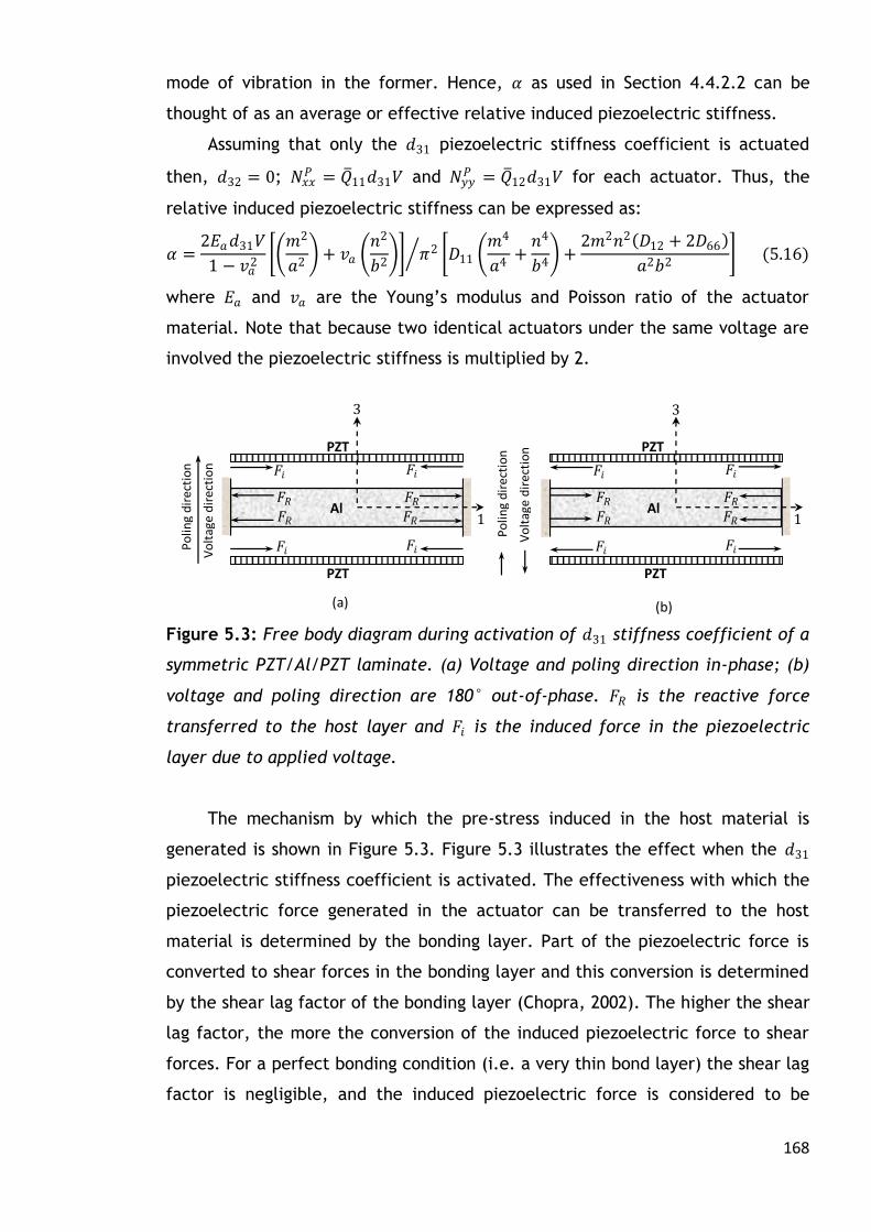
168

(a) (b)

PZT

Po

ling

dir

ecti

on

Vo

ltag

e d

irec

tio

n

𝐹𝑖 𝐹𝑖

𝐹𝑅

𝐹𝑅

𝐹𝑖 𝐹𝑖

𝐹𝑅

𝐹𝑅 Al

PZT

3

1

Po

ling

dir

ecti

on

Vo

ltag

e d

irec

tio

n

𝐹𝑖 𝐹𝑖

𝐹𝑅

𝐹𝑅

𝐹𝑖 𝐹𝑖

𝐹𝑅

𝐹𝑅 Al

PZT

PZT

3

1

mode of vibration in the former. Hence, 𝛼 as used in Section 4.4.2.2 can be

thought of as an average or effective relative induced piezoelectric stiffness.

Assuming that only the 𝑑31 piezoelectric stiffness coefficient is actuated

then, 𝑑32 = 0; 𝑁𝑥𝑥𝑃 = 𝑄 11𝑑31𝑉 and 𝑁𝑦𝑦

𝑃 = 𝑄 12𝑑31𝑉 for each actuator. Thus, the

relative induced piezoelectric stiffness can be expressed as:

𝛼 =2𝐸𝑎𝑑31𝑉

1 − 𝑣𝑎2 𝑚2

𝑎2 + 𝑣𝑎

𝑛2

𝑏2 𝜋2 𝐷11

𝑚4

𝑎4+𝑛4

𝑏4 +

2𝑚2𝑛2 𝐷12 + 2𝐷66

𝑎2𝑏2 (5.16)

where 𝐸𝑎 and 𝑣𝑎 are the Young’s modulus and Poisson ratio of the actuator

material. Note that because two identical actuators under the same voltage are

involved the piezoelectric stiffness is multiplied by 2.

Figure 5.3: Free body diagram during activation of 𝑑31 stiffness coefficient of a

symmetric PZT/Al/PZT laminate. (a) Voltage and poling direction in-phase; (b)

voltage and poling direction are 180° out-of-phase. 𝐹𝑅 is the reactive force

transferred to the host layer and 𝐹𝑖 is the induced force in the piezoelectric

layer due to applied voltage.

The mechanism by which the pre-stress induced in the host material is

generated is shown in Figure 5.3. Figure 5.3 illustrates the effect when the 𝑑31

piezoelectric stiffness coefficient is activated. The effectiveness with which the

piezoelectric force generated in the actuator can be transferred to the host

material is determined by the bonding layer. Part of the piezoelectric force is

converted to shear forces in the bonding layer and this conversion is determined

by the shear lag factor of the bonding layer (Chopra, 2002). The higher the shear

lag factor, the more the conversion of the induced piezoelectric force to shear

forces. For a perfect bonding condition (i.e. a very thin bond layer) the shear lag

factor is negligible, and the induced piezoelectric force is considered to be

169

completely transferred to the host structure (Chopra, 2002). In the present

analysis a perfect bonding condition is assumed between the Al and PZT layers.

A voltage applied in the poling direction of the piezoactuator (positive

voltage) tends to shrink the piezoactuator layer because the 𝑑31 stiffness

coefficient is negative (Preumont, 2011). An equal reactive in-plane tensile

force is generated on the host layer to which the piezoactuator layer is bonded,

and because the plate is restrained from planar displacements a tensile pre-

stress is created in the plate (i.e. 𝛼 < 0). This gives rise to the well known stress

stiffening effect (see Figure 5.3a). For the two piezoactuator layers bonded on

the top and bottom surfaces of the host layer the total pre-stress created in the

plate is the sum of the stresses induced by each actuator. Similarly, if the

voltage is applied opposite to the poling direction (negative voltage) an in-plane

tensile force is generated in the actuator layers and a reactive in-plane

compressive force is created on the host layer resulting in a compressive pre-

stress (𝛼 > 0). The implication is that the plate becomes more compliant to

transverse load (see Figure 5.3b). If the voltage applied at the top piezoactuator

layer is equal and opposite to that applied at the bottom piezoactuator layer,

then the plate undergoes pure bending. This situation is not necessary for the

present investigation, but further information can be found in Chopra (2002) and

Lazarus (1989).

The equation of the impactor is the same as equation (4.44b) i.e.

𝑊 2 = −𝐹(𝑡)/𝑚𝑖 (5.17)

where 𝑊2 is the displacement of the impactor and 𝑚𝑖 is the mass of the

impactor. The impact force 𝐹 𝛿(𝑡) ≥ 0 is estimated using the elastoplastic

contact model presented in Section 3.2. The local indentation is given as

𝛿(𝑡) = 𝑊2 −𝑊1.

5.4.2 Results and discussions on mitigation of elastoplastic impact

effects using PZT/Al/PZT plate

The above models were used to investigate the low-velocity impact

response of a PZT/Al/PZT plate subjected to induced active pre-stress (tensile

or compressive). The mechanical properties of the Al and PZT layers are the

same as in Table 4.5, given in Section 4.4.2.2. The applied voltage is ± 200 [V]

and the piezoelectric stiffness coefficient used in the simulations is 𝑑31 =

170

−254 × 10−12[𝑚/𝑉] (Oguamanam et al, 1998). The planar dimension of the plate

is 300 x 300 [mm2] and the thicknesses of the Al and PZT layers are 2.40 [mm]

and 50.0 [µm] respectively. The impactor mass, initial velocity, and radius are

0.30 [kg], 0.50 [m/s], and 10 [mm] respectively. The impactor is made of steel

and the material properties are given in Section 4.4.2.2.

The plate has a length to thickness ratio of 120, which means that the plate

is highly transversely flexible. Such high transverse flexibility (i.e. very thin

plate) is required if the induced piezoelectric stress is to have a significant

effect on the transverse response of the plate (Oguamanam et al, 1998). From

an analytical point of view, the solution of the complete impact model, when a

plate with high transverse flexibility is involved, is more complicated because

the solution is very sensitive to the physical input parameters and the number of

vibration modes used to approximate the solution. Consequently, in many cases

a convergent numerical solution can be difficult to obtain. One way to overcome

this difficulty is to use fewer vibration modes in the solution, though this comes

at the cost of reduced accuracy. In Section 4.4.2.2 it was shown that 9 modes of

vibration is sufficient to produce a convergent solution for large mass impact of

a thin to moderately thick plate. Hence, equations (5.14) and (5.17) have been

solved for m = n = 5 (i.e. 9 vibration modes) because the impact response for the

cases investigated here exhibit typical characteristics of large mass impact i.e.

the displacements of the impactor and plate at the point of impact are almost

the same. This does not mean that improved accuracy cannot be obtained with

more than 9 vibration modes, but that 9 vibration modes are considered to be

sufficient for the present purpose, i.e. to demonstrate the effect of actively

induced pre-stress on the subsequent impact damage.

Three cases were considered namely: (a) no pre-stress (b) an induced

tensile pre-stress and (c) an induced compressive pre-stress. The applied voltage

in each case are 0 [V], 200 [V], and – 200 [V] respectively. In solving the models

(equations (5.14) and (5.17)) the elastic loading response is terminated at the

point where the dynamic indentation is equal to the static yield indentation (see

Section 3.2) and the elastoplastic loading response is terminated when the

impactor velocity is zero. The unloading response is terminated at the point

where the indentation is equal to the static permanent indentation. This is

consistent with the assumption that the impact force during low- to medium-

velocity impacts can be estimated from static contact models (Johnson, 1985).

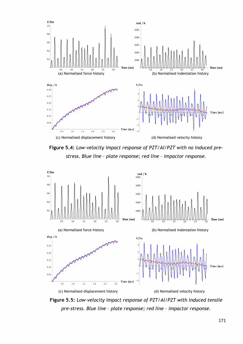
171

Figure 5.4: Low-velocity impact response of PZT/Al/PZT with no induced pre-

stress. Blue line – plate response; red line – impactor response.

Figure 5.5: Low-velocity impact response of PZT/Al/PZT with induced tensile

pre-stress. Blue line – plate response; red line – impactor response.

0.5 1.0 1.5 2.0 2.5 3.0Time ms

0.2

0.4

0.6

0.8

1.0

FFm

0.5 1.0 1.5 2.0 2.5 3.0Time ms

0.005

0.010

0.015

0.020

0.025

ind. h

0.5 1.0 1.5 2.0 2.5 3.0Tim e m s

0.05

0.10

0.15

0.20

0.25

0.30

di sp. h

Impactor

Plate0.5 1.0 1.5 2.0 2.5 3.0

Tim e m s

3

2

1

1

2

3

VVo

Impactor

Plate

0.5 1.0 1.5 2.0 2.5 3.0Time ms

0.2

0.4

0.6

0.8

1.0

FFm

0.5 1.0 1.5 2.0 2.5 3.0Time ms

0.005

0.010

0.015

0.020

0.025

ind. h

0.5 1.0 1.5 2.0 2.5 3.0Tim e m s

0.05

0.10

0.15

0.20

0.25

di sp. h

Impactor

Plate

0.5 1.0 1.5 2.0 2.5 3.0Tim e m s

2

1

1

2

3

VVo

Impactor

Plate

(c) Normalised displacement history (d) Normalised velocity history

(a) Normalised force history (b) Normalised indentation history

(c) Normalised displacement history


(d) Normalised velocity history

172

Plots for the time histories of the impact force, indentation, and the

impactor and plate displacements and velocities for the three cases (a – c) are

shown in Figures 5.4 – 5.6. The force history is normalised with respect to the

maximum impact force while the displacements and indentation histories are

normalised with respect to the total thickness of the plate. The velocity history

is normalised with respect to the initial impact velocity. The plots reveal that

the impact response is mainly dominated by the global response (i.e. the

displacement of the plate is large compared to the indentation), which is the

distinguishing characteristic of a large mass impact. This observation is

noteworthy given that the impactor-plate mass ratio for the present example is

0.46 and the impact event can therefore not be classified as a large mass impact

based on the frequently used ‘Olsson’s mass criterion’ i.e. mass ratio ≥ 2 for

large mass impact (Olsson, 2000). It seems that Olsson’s mass criterion may be

limited by the length to thickness ratio because the plate under investigation has

a ratio of 120 and its response is globally dominated for the impact event

considered even though the mass ratio is well below what would be expected to

produce a globally dominated response according to Olsson’s mass criterion.

Figure 5.6: Low-velocity impact response of PZT/Al/PZT with induced

compressive pre-stress. Blue line – plate response; red line – impactor response.

0.5 1.0 1.5 2.0 2.5 3.0Time ms

0.2

0.4

0.6

0.8

1.0

FFm

0.5 1.0 1.5 2.0 2.5 3.0Time ms

0.005

0.010

0.015

0.020

0.025

0.030

ind. h

0.5 1.0 1.5 2.0 2.5 3.0Tim e m s

0.05

0.10

0.15

0.20

0.25

0.30

di sp. h

Impactor

Plate

0.5 1.0 1.5 2.0 2.5 3.0Tim e m s

2

1

1

2

3

4

VVo

Impactor

Plate

(c) Normalised displacement history (d) Normalised velocity history


173

The local indentation (Figures 5.4b, 5.5b, and 5.6b) is relatively small

compared to the displacement of the impactor and the plate (Figures 5.4c, 5.5c,

and 5.6c), which are similar. This means that most of the initial impact energy is

converted into vibration energy in the plate. The velocity histories (Figures 5.4d,

5.5d, and 5.6d) show a gradual dissipation of the initial impact energy, while at

the same time the highly dynamic interactions between the impactor and the

plate (see Figures 5.4c, 5.5c, and 5.6c) result in multiple impacts (Figures 5.4a,

5.5a, and 5.6a). The maximum impact force and indentation occur at the 19th

impact in all three cases.

Table 5.1: Modal dependence of mechanical and piezoelectric stiffnesses

Modes Mechanical bending

stiffness, 𝑲 [N/mkg]

Relative induce piezoelectric

stiffness, 𝜶 [-] m n

1 1 6.725 × 105 ± 0.2093980

1 3 1.681 × 107 ± 0.0238391

1 5 1.136 × 108 ± 0.0081014

3 1 1.681 × 107 ± 0.0599199

3 3 5.447 × 107 ± 0.0232664

3 5 1.943 × 108 ± 0.0091963

5 1 1.136 × 108 ± 0.0241136

5 3 1.943 × 108 ± 0.0154387

5 5 4.203 × 108 ± 0.0083759

In Section 5.4.1, expressions for the mechanical bending and induced

piezoelectric stiffnesses were derived (see equations (5.15) and (5.16)) and

shown to depend on the vibration mode. Table 5.1 shows the modal dependence

of the mechanical bending and induced piezoelectric stiffnesses for the nine

vibration modes used in approximating the solution of the impact response, for

an applied voltage of ± 200 [V]. The induced piezoelectric stiffnesses shown in

Table 5.1 are negative for tensile pre-stress and positive for compressive pre-

stress. The results show that the induced piezoelectric stiffness is most effective

at the fundamental mode of vibration. At higher vibration modes, both the

effect of the mechanical bending and induced piezoelectric stiffnesses continue

to diminish. The effect of the induced piezoelectric stiffnesses can be increased

by using a thinner plate, i.e. a higher length to thickness ratio (Oguamanam et

al, 1998) or by increasing the applied voltage. The increase in the voltage is

limited by the dielectric breakdown voltage of the actuator and the critical

buckling load of the plate.

174

Table 5.2: Effect of actively induced pre-stress on critical impact parameters

Impact parameters No pre-stress Tensile

pre-stress

Compressive

pre-stress

Maximum contact force , 𝐹𝑚 [kN] 2.208 1.907 2.570

Maximum indentation, 𝛿𝑚 [µm] 44.85 40.82 49.47

Permanent indentation, 𝛿𝑓 [µm] 4.34 8.15 10.97

Duration of elastic loading response

[µs] 0 – 3.95 0 – 3.95 0 – 3.95

Duration of elastoplastic loading

response [µs] 3.95 – 3151.04

3.95 –

3023.12

3.95 –

3284.86

Duration of unloading response [µs] 3151.04 –

3194.69

3023.12 –

3055.87

3284.86 –

3309.94

Duration of impact response [ms] 3.195 3.056 3.310

Time at which maximum force

occurred [ms] 2.593 2.596 2.590

Final rebound velocity [m/s] 0.0491 0.0691 0.0649

Number of impacts [-] 23 22 24

The effect of active pre-stressing on the impact response of the

PZT/Al/PZT plate is summarised in Table 5.2. The results of critical impact

parameters are compared for the three cases. These impact parameters are

considered to be critical because they determine the damage size and shock

effect of the impact, and the amount of energy absorbed by the plate. The

nominal case used for comparison is the impact without pre-stress (column 2).

The induced tensile pre-stress resulted in a reduction of the maximum impact

force by 13.63% while the induced compressive pre-stress increased the

maximum impact force by 16.39%. For single impact events, application of a

tensile pre-stress produces a maximum impact force higher than the nominal

case (no pre-stress), while a compressive pre-stress produces a maximum impact

force lower than the nominal case (see Figure 4.27). In contrast, the present

impact event is characterised by multiple impacts and the complex nature of

such an impact event can produce a higher maximum impact force for either

tensile or compressive pre-stress condition. In the present investigation the

compressive pre-stress condition produced a higher maximum impact force (see

Table 5.2). Overall, the effect of the induced tensile pre-stress appears to be

more beneficial than the effect of the compressive pre-stress, and gives a better

mitigation of elastoplastic impact effects in terms of a lower maximum impact

force, a smaller number of impacts and a smaller impact energy absorption by

175

the plate (as shown by the final rebound velocity). The only apparent drawback

of the effect of the induced tensile pre-stress is that it produced a permanent

indentation that is higher than the nominal case.

The impact durations for the impact stages of all three cases reveal that

the impact response is dominated by the elastoplastic loading response. The

elastic loading response occurs in less than 0.2% of the impact duration while the

unloading response occurs in about 1.0% of the impact duration. The implication

is that the elastoplastic loading response takes place for more than 98.0% of the

impact duration. This underscores the importance of using elastoplastic contact

models that account for post-yield effects in impact analysis. Furthermore,

elastoplastic contact models that account for post-yield effects can be used to

predict the permanent indentation, as in the present analysis, which may be

difficult to obtain otherwise.

The total mass of the PZT layers in the PZT/Al/PZT plate studied is 0.0684

[kg], just 11.73% of the mass of the Al layer (0.5832 [kg]). The maximum impact

force predicted when a tensile pre-stress is actively induced at an applied

voltage of 200 [V] is 1.907 [kN] (see Table 5.2). If the PZT layers are taken off

and a passive Al plate of equivalent thickness as the total thickness of the

PZT/Al/PZT plate is subjected to the same impact conditions, then the

maximum impact force predicted would be 2.444 [kN]. Since the mass of the

passive Al plate is 0.6075 [kg] and the mass of the PZT/Al/PZT plate is 0.6516

[kg], it can be concluded that a 7.26% increase in the mass of the plate (i.e.

when the PZT/Al/PZT plate is used instead of the Al plate) gives rise to a 21.97%

reduction in the maximum impact force, when a tensile pre-stress is actively

induced at an applied voltage of 200 [V]. On the other hand, a comparison for

the case of PZT/Al/PZT with no pre-stress and with tensile pre-stress (see Table

5.2) show that the maximum impact force is reduced by 13.63%, when a tensile

pre-stress is induced at a voltage of 200 [V]. These trade-offs could be further

enhanced by optimising the effect of the induced pre-stress. The optimisation of

the induced pre-stress is beyond the scope of the present work and is left for

future research.

176

5.5 Implementation issues of the proposed strategy for

active impact damage mitigation

So far the focus of this chapter has been the investigation of the effect of

active pre-stress on the low-velocity impact response of a PZT/Al/PZT laminate

plate using analytical models that account for permanent indentation of the

local response. It was shown that both tensile and compressive pre-stress could

influence the impact response significantly and for the particular impact event

investigated, an induced tensile pre-stress produced better mitigation of the

elastoplastic impact effects than an induced compressive pre-stress. The

proposed strategy of active pre-stressing using piezoceramic actuators can be

used to develop a controller for optimised impact damage mitigation. The

primary objective of such a control algorithm would be to actively redistribute

the impact energy absorbed by the target structure to meet pre-determined

impact damage mitigation solutions. The pre-determined impact damage

mitigation solutions include an increase in the local damage in favour of less

structural damage (Yigit and Christoforou, 2000), a reduction of the energy

absorbed by the structure in favour of higher rebound energy (impact

resistance), and an elongation of the impact duration by allowing absorption of

more vibration energy in favour of reducing the shock effect of the impact. For

instance, during impact of runway debris on an airplane the local indentation

effects may be critical and are of concern, whereas vibrations are small and

harmless. In this case it would be useful to have the structure absorb more

vibration energy in favour of less local indentation. Another example may be the

impact of a car body and a pedestrian; here it would be beneficial to reduce the

shock effect of the impact and enhance the vibration energy absorption of the

structure.

Basically, the impact energy of a low-velocity impact can be dissipated as

local indentation energy, vibration energy, and rebound energy of the impactor.

Other possible mechanisms of dissipation such as sound and friction energy are

negligible (Johnson, 1985; Abrate, 1998). The indentation energy produces local

damage effects such as permanent indentation, cracks and perforation, while

the vibration energy produces global damage effects such as delamination and

noise. Altering the structural stiffness can influence the energy dissipation

177

mechanism and this can be achieved through actively induced pre-stress, as

demonstrated above.

The practical implementation of induced pre-stress using a controller

design to actively mitigate impact damage effects would require remote sensing

of the impactor parameters before the impact takes place. Required impactor

parameters include mass, velocity, size, contact geometry and material

composition. Even though it may not be practically possible to obtain a precise

estimate of the impactor details in real time, very good estimates can be

obtained using available remote sensing technologies such as high speed camera,

LIDAR (light detection and ranging), radar and sonic sensors. These technologies

are already implemented in autonomous vehicles and space technologies for

obstacle avoidance and foreign object detection and analysis (Bicho et al, 2000;

Mujica, 2014). Additionally, the control system would require a database of

materials to estimate the impactor’s material properties once the composition

of the impactor had been determined from the remotely sensed information.

After the impactor parameters are estimated, the impact models presented

in this chapter could be used to estimate the passive impact response of the

smart plate, and then, the critical response parameters could be matched with

the predetermined control objectives in order to estimate the input voltage for

active mitigation. Very high speed processors with parallel computing abilities

that can analyse the remotely sensed information and determine the control

input voltage in fractions of a second are required to achieve this. Since remote

sensing can be achieved while the impactor is still a few seconds away (Mujica,

2014), it is concluded that active pre-stressing as a strategy for mitigation of

elastoplastic impact effects would seem to be practically feasible.

Although the focus of the present chapter has been on the mitigation of

elastoplastic impact effects using a symmetric sandwich laminate (PZT/Al/PZT),

the trimorph plate configuration with piezoelectric actuator (PZT) and sensor

(PVDF) layers integrated on a host layer can also be used for active pre-

stressing. In this case, the sensor layer could be use for in situ sensing and

provide information for active control of the post-impact response. This

arrangement might be useful in a situation where active damping can be used to

suppress the post-impact vibration in order to forestall global response damage

effects. Since the actuator is in an unsymmetric laminate arrangement, its

activation would produce an in-plane force and a bending moment. The bending

178

moment would produce an initial bending prior to impact and the in-plane force

would produce a pre-stress in the plate. Actuation in this trimorph arrangement

will most likely be less effective than in the PZT/Al/PZT arrangement with two

actuators and no bending moment. Hence, in situations where in situ sensing

may be needed, other symmetric arrangements such as PVDF/PZT/Al/PZT/PVDF

or (PZT)2/Al/(PZT)2 could be investigated. In the latter case, the outermost PZT

layers could be used as in situ sensors.


In this chapter the vibration models discussed in chapter two, and the new

elastoplastic contact model formulated in chapter 3, were combined with linear

piezoelectric theory to formulate impact models that were used to investigate

the effect of actively induced pre-stress on the impact response of a smart

plate. A symmetric laminate was modelled and investigated. Simulations using

the models demonstrated that actively induced pre-stress can influence the

impact response of the symmetric laminate plate significantly. In this case

study, it was found that a significant reduction in maximum impact force can be

achieved by the smart plate. It was therefore proposed that actively induced

pre-stress could potentially be a very useful mitigation strategy against

elastoplastic impact effects. Also, the issues associated with the practical

implementation of a controller designed to mitigate elastoplastic impact effects

using the proposed active pre-stress strategy were discussed. It was argued that

due to the availability of very efficient remote sensors and high speed processors

with parallel computing features, such a controller is practically feasible.

179

CHAPTER SIX

CONCLUSIONS AND RECOMMENDATIONS

6.1 Conclusions of thesis

The elastoplastic impact response of a multilayered plate, described here

as a trimorph plate, has been investigated using analytical models. To obtain

more accurate results and details of the elastoplastic impact response an impact

modelling approach known as the complete modelling approach was used to

formulate the impact model of the trimorph plate. This approach combines the

equations of motion of the contacting bodies, in this case the trimorph plate and

a spherical impactor, and the compliance model for the local contact mechanics

to formulate the impact model. Hence, in developing the research presented

within this thesis the vibration characteristics of the trimorph plate was

investigated first. A key finding from this investigation is that the vibration

response of the trimorph plate is dependent on the arrangement of its layers.

Next, a novel elastoplastic compliance model for impact analysis was formulated

and validated using published experimental results. This was followed by

detailed investigations on the elastoplastic impact response of rectangular

plates, in which the local contact mechanics was accounted for using the newly

formulated elastoplastic compliance model. Based on the observations and

conclusions of the elastoplastic impact analysis of the trimorph plate, a newly

proposed strategy for mitigation of elastoplastic impact effects, i.e. plastic

deformation and/or damage, was investigated.

The elastoplastic response of both transversely inflexible and transversely

flexible rectangular plates during impact of a spherical mass was studied. For

transversely inflexible plates, the impact models were formulated using the

equation of motion of the impactor and the new compliance model. Results from

the simulation of the impact models for transversely inflexible plates showed

that the elastic loading response has a negligible influence on the impact

response when the maximum penetration is located well into the linear

elastoplastic regime. It was observed that the fraction of the initial impact

energy absorbed as plastic deformation increased as the initial impact velocity

increased. Additionally, an efficient algorithm capable of solving the nonlinear

models of a half-space impact was formulated. The algorithm, which has been

180

called force-indentation linearisation method (FILM), is simple, inherently stable

and converges within a few iterations; typically between five and ten. The FILM

algorithm solves the nonlinear models of a half-space impact with the same

relative ease irrespective of the complexity of the compliance model used to

estimate the impact force. The results obtained using the FILM algorithm showed

an excellent match with results obtained from direct numerical integration of

the nonlinear models governing the half-space impact. Also, the FILM algorithm

proved to be accurate when applied to solving the nonlinear model for elastic

impact response of an infinitely large transversely flexible plate. Unlike the case

of a transversely inflexible plate impact where the FILM algorithm is completely

analytical, it becomes semi-analytical when applied to solve the nonlinear

impact model of a transversely flexible plate. This is because the time at the

boundaries of each discretisation is now determined using an implicit

formulation. The implication is that more iteration is required to obtain accurate

solutions to the nonlinear impact models of transversely flexible plates.

Investigations on the elastoplastic impact response of a transversely

flexible plate were carried out using the trimorph plate. The investigations were

limited to low-velocity large mass impact. A convergence test on the solution of

the trimorph plate impact model showed that the first nine modes of vibration

are sufficient to guarantee accurate results. The effect of transverse shear

deformation, compliance model used to estimate the impact force, impactor

mass, impactor size, initial impact velocity, plate thickness, plate aspect ratio

and bending stiffness, on the elastoplastic impact response of a typical trimorph

plate configuration was investigated. The results showed that the effect of

transverse shear deformation on the elastoplastic impact response of the

trimorph plate is negligible. All the other impact parameters considered were

shown to have a significant influence. The response characteristics influenced by

these impact parameters include: oscillations in the impact force history,

maximum impact force, impact duration and permanent indentation. The

permanent indentation is indicative of the amount of plastic deformation and/or

local damage that occurred during the impact loading (Majeed et al, 2012).

Analysis of the effect of transverse bending stiffness on the elastoplastic

impact response of the trimorph plate showed that the flexibility of the plate

can influence its elastoplastic response significantly. This observation, which is

supported by previous studies (Christoforou and Yigit, 1998b) was used to

181

investigate a newly proposed strategy for active mitigation of elastoplastic

impact effects. The strategy is based on using a bonded piezoelectric layer to

actively induce a state of pre-stress in the substrate layer. The pre-stress

induced in the substrate layer influences the flexibility of the plate, which in

turn influences the elastoplastic impact response. This strategy was investigated

for a PZT/Al/PZT plate configuration using an impact model that accounts for

the effect of induced piezoelectric pre-stress on the transverse flexibility of the

plate. This effect was captured in the impact model through a non-dimensional

parameter called relative induced piezoelectric stiffness. The latter is defined

here as the ratio of the total induced piezoelectric stiffness to the mechanical

bending stiffness of the plate.

Simulations of the impact model were carried out for both tensile and

compressive pre-stress states created by an applied voltage of 200 volts. The

results obtained were compared to a no pre-stress state and the comparison

showed that the elastoplastic impact effects such as permanent indentation can

be significantly altered through induced piezoelectric pre-stress. This strategy

can be used to design a controller for active mitigation of elastoplastic impact

effects. The input information required by the controller (i.e. impactor speed,

mass, size and material composition) would be obtained by remote sensing

technology such as camera and radar sensors. The use of remote sensors would

avail the piezoactuators with sufficient time to provide active response to an

imminent impact. However, in situ sensors can also be used to provide

information for active control of the post-impact response of the plate.

Additionally, the proposed strategy for active mitigation of elastoplastic impact

effects can be used together with existing passive mitigation strategies to

further enhance the impact damage mitigation capacity of structures. The

potential benefits of the application of the proposed mitigation strategy include

cost savings, reduction of risk to life and structural survivability/re-usability.

In conclusion, analytical models for impact analysis of structures should

account for elastoplastic effects since it has been sufficiently demonstrated in

this thesis and in the literature (Johnson, 1985; Goldsmith, 2001; Majeed et al,

2012) that significant elastoplastic deformation occurs at typical low-velocity

impacts. Furthermore, neglecting elastoplastic effects in impact analysis could

introduce significant errors in the predicted impact response (Abrate, 1998) and

limit the details that can be obtained. The work presented in this thesis provides

182

an insightful analysis of the elastoplastic impact response of both transversely

inflexible and transversely flexible rectangular plates. The modelling of the local

contact mechanics for low-velocity impact events has been improved and

particular attention has been paid to the solution of nonlinear impact models,

which are usually difficult to solve. New solution methods that are easy to

implement are developed, especially for transversely inflexible plate impact,

and the NDSolve function in Mathematica™ is shown to be an efficient numerical

integration tool for solving nonlinear impact models. Finally, investigations on

active mitigation of elastoplastic impact effects reveal its viability and reinforce

the need for more research activity in this area, which is largely unexplored at

present.

6.2 Recommendations for future research

The methodology of the present research is to use analytical models to

investigate the elastoplastic response of rectangular plates subjected to

spherical object impact, and to explore the possibility of active mitigation of

elastoplastic impact effects in transversely flexible plates. In applying this

methodology, a traditional impact modelling approach, which has been proven

to produce reliable results for over a century, has been applied. The traditional

approach is to use a well validated static compliance model to estimate the

impact force of a rate-independent impact event i.e. low- to medium-velocity

impact. Once the static compliance model is substituted for the force in the

equations of motion of the contacting bodies and the indentation is defined as

the relative displacement of the contacting bodies, the impact model so

obtained can be considered to be reliable. However, there are two major areas

of the present work where further validation would give credence to the

quantitative analysis.

The trimorph plate is a composite laminate consisting of three layers with

different material properties. This means that yielding in the trimorph plate is

quite complex. Furthermore, effective transverse properties of the trimorph

plate are needed for the analytical models. The effective transverse properties

have been estimated using the strength of materials approach, which is an

approximate method. It is therefore necessary to verify the analytical results of

the elastoplastic impact response of the trimorph plate independently. Such

183

validation can be carried out using finite element models developed in software

packages like ABAQUS, ANSYS and COMSOL. Two finite element models can be

tested and compared with the analytical results. The first finite element model

would require homogenisation of the trimorph plate to obtain an equivalent

monolithic plate with effective properties, and then, using the equivalent

monolithic plate for elastoplastic analysis of a spherical impact. This approach

was used by Majeed et al (2012) to investigate the elastoplastic impact response

of a very thick carbon-epoxy laminate subjected to spherical impact. The second

finite element model would require modelling the trimorph plate with its

different layers, and using the composite trimorph plate for spherical impact

analysis. Since an elastoplastic impact analysis is desired, post-yield stress-strain

data for each material that make-up the trimorph plate would be needed for the

finite element models. Such data are readily available from the literature.

The second area of the present work that require further validation is the

modelling of the induced piezoelectric stiffness created by actively pre-stressing

the host layer of the PZT/Al/PZT sandwich plate. Basic piezoelectric theory has

been applied in the present research to derive the model for estimating this

effect. A finite element model can be built to validate the estimation of this

effect, and to demonstrate quantitatively the extent of elastoplastic impact

damage mitigation that is possible.

An alternative validation approach to finite element modelling is

experimentation. Although impact experiments are generally simple, an

experiment to investigate the active mitigation of elastoplastic impact effects is

not likely to be that simple. A relatively simpler experiment would be to

investigate the elastoplastic impact response of the trimorph plate. This latter

experimental investigation would involve two main stages namely: (a)

preparation of the target specimen, which is a composite laminate plate, and (b)

setting up the experimental rig. The impactor should not be controllable as

obtained in many existing drop-weight impact testing machines e.g. a

Zwick/Roell HIT230F drop weight tester. Rather, the impactor should be

dropped freely from a height and allowed to rebound as a result of the impact

resistance of the plate specimen, just like the experiments of Kharaz and

Gorham (2000). Difficulties with the experiment may arise due to the need to

achieve the correct boundary conditions and measure the permanent indentation

184

after impact. Nevertheless, a carefully planned experiment remains a preferable

and more reliable means of validating the quantitative results.

Due to time constraint on the present research none of the validation

exercises discussed above was conducted. However, any of the validation

exercises discussed above could be carried out as the next logical step in

continuing with the work presented in this thesis. The boundary and loading

conditions used in this thesis are simply-supported on all edges (SSSS) and

concentrated point load respectively. Further research can be carried out to

improve the analytical models presented in this thesis to incorporate more

realistic boundary and loading conditions. The impact load for a spherical impact

can be more realistic represented by a load distributed over a circular patch

(Nosier et al, 1994). Other boundary conditions such as clamped on all edges

(CCCC), clamped-free (CFCF or CCFF) and elastically-restrained edges, to

mention but a few, can be investigated using the analytical models presented in

this thesis.

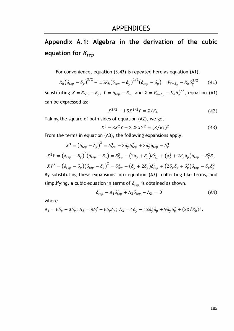
185

APPENDICES

Appendix A.1: Algebra in the derivation of the cubic

equation for 𝜹𝒕𝒆𝒑

For convenience, equation (3.43) is repeated here as equation (A1).

𝐾𝑕 𝛿𝑡𝑒𝑝 − 𝛿𝑦 3 2

− 1.5𝐾𝑕 𝛿𝑡𝑒𝑝 − 𝛿𝑦 1 2

𝛿𝑡𝑒𝑝 − 𝛿𝑝 = 𝐹𝛿=𝛿𝑝 − 𝐾𝑕𝛿𝑦3 2 (𝐴1)

Substituting 𝑋 = 𝛿𝑡𝑒𝑝 − 𝛿𝑦 , 𝑌 = 𝛿𝑡𝑒𝑝 − 𝛿𝑝 , and 𝑍 = 𝐹𝛿=𝛿𝑝 − 𝐾𝑕𝛿𝑦3 2

, equation (A1)

can be expressed as:

𝑋3 2 − 1.5𝑋1 2 𝑌 = 𝑍 𝐾𝑕 (𝐴2)

Taking the square of both sides of equation (A2), we get:

𝑋3 − 3𝑋2𝑌 + 2.25𝑋𝑌2 = 𝑍 𝐾𝑕 2 𝐴3

From the terms in equation (A3), the following expansions apply.

𝑋3 = 𝛿𝑡𝑒𝑝 − 𝛿𝑦 3

= 𝛿𝑡𝑒𝑝3 − 3𝛿𝑦𝛿𝑡𝑒𝑝

2 + 3𝛿𝑦2𝛿𝑡𝑒𝑝 − 𝛿𝑦

3

𝑋2𝑌 = 𝛿𝑡𝑒𝑝 − 𝛿𝑦 2 𝛿𝑡𝑒𝑝 − 𝛿𝑝 = 𝛿𝑡𝑒𝑝

3 − 2𝛿𝑦 + 𝛿𝑝 𝛿𝑡𝑒𝑝2 + 𝛿𝑦

2 + 2𝛿𝑦𝛿𝑝 𝛿𝑡𝑒𝑝 − 𝛿𝑦2𝛿𝑝

𝑋𝑌2 = 𝛿𝑡𝑒𝑝 − 𝛿𝑦 𝛿𝑡𝑒𝑝 − 𝛿𝑝 2

= 𝛿𝑡𝑒𝑝3 − 𝛿𝑦 + 2𝛿𝑝 𝛿𝑡𝑒𝑝

2 + 2𝛿𝑦𝛿𝑝 + 𝛿𝑝2 𝛿𝑡𝑒𝑝 − 𝛿𝑦𝛿𝑝

2

By substituting these expansions into equation (A3), collecting like terms, and

simplifying, a cubic equation in terms of 𝛿𝑡𝑒𝑝 is obtained as shown.

𝛿𝑡𝑒𝑝3 − Λ1𝛿𝑡𝑒𝑝

2 + Λ2𝛿𝑡𝑒𝑝 − Λ3 = 0 (A4)

where

Λ1 = 6𝛿𝑝 − 3𝛿𝑦 ; Λ2 = 9𝛿𝑝2 − 6𝛿𝑦𝛿𝑝; Λ3 = 4𝛿𝑦

3 − 12𝛿𝑦2𝛿𝑝 + 9𝛿𝑦𝛿𝑝

2 + 2𝑍 𝐾𝑕 2.

186

Appendix A.2: Deformation work during contact loading

Using equations (3.26) – (3.30) the work done in each of the three loading

regimes can be obtained as shown.

Work done during the elastic loading regime

𝑊𝑒 = 𝐹𝑒

𝛿𝑦

0

𝑑𝛿 = 𝐾𝑕𝛿3 2

𝛿𝑦

0

𝑑𝛿 = 0.4𝐾𝑕𝛿𝑦5 2 (𝐴5)

Work done during the nonlinear elastoplastic loading region

𝑊𝑒𝑝𝐼 = 𝐹𝑒𝑝

𝐼𝛿𝑡𝑒𝑝

𝛿𝑦

𝑑𝛿 = 𝐾𝑕 𝛿 − 𝛿𝑦 3 2

+ 𝐾𝑕𝛿𝑦3 2

𝛿𝑡𝑒𝑝

𝛿𝑦

𝑑𝛿

= 0.4𝐾𝑕 𝛿𝑡𝑒𝑝 − 𝛿𝑦 5 2

+ 𝐾𝑕𝛿𝑦3 2 𝛿𝑡𝑒𝑝 − 𝛿𝑦 (𝐴6)

Work done during the linear elastoplastic loading region

𝑊𝑒𝑝𝐼𝐼 = 𝐹𝑒𝑝

𝐼𝐼𝛿𝑝

𝛿𝑡𝑒𝑝

𝑑𝛿 = 𝐾𝑙 𝛿 − 𝛿𝑡𝑒𝑝 + 𝐾𝑕 𝛿𝑡𝑒𝑝 − 𝛿𝑦 3 2

+ 𝛿𝑦3 2

𝛿𝑝

𝛿𝑡𝑒𝑝

𝑑𝛿

= 0.5𝐾𝑙 𝛿𝑝 − 𝛿𝑡𝑒𝑝 2

+ 𝐾𝑕 𝛿𝑡𝑒𝑝 − 𝛿𝑦 3 2

+ 𝛿𝑦3 2 𝛿𝑝 − 𝛿𝑡𝑒𝑝 (𝐴7)

Work done during the fully plastic loading regime

𝑊𝑓𝑝 = 𝐹𝑓𝑝

𝛿𝑚

𝛿𝑝

𝑑𝛿 = 𝐾𝑝 𝛿 − 𝛿𝑝 + 𝐹𝑝 𝛿𝑚

𝛿𝑝

𝑑𝛿

= 0.5𝐾𝑝 𝛿𝑚 − 𝛿𝑝 2

+ 𝐹𝑝 𝛿𝑚 − 𝛿𝑝 (𝐴8)

Using equations (A5) – (A8), the following work done can be determined.

Work done up to the end of the elastic loading regime, 𝑊𝑦

𝑊𝑦 = 𝑊𝑒 = 0.4𝐾𝑕𝛿𝑦5 2 (𝐴9)

Work done up to the end of region I, 𝑊𝑡𝑒𝑝

𝑊𝑡𝑒𝑝 = 𝑊𝑦 + 𝑊𝑒𝑝𝐼 = 0.4𝐾𝑕𝛿𝑦

5 2 + 0.4𝐾𝑕 𝛿𝑡𝑒𝑝 − 𝛿𝑦 5 2

+ 𝐾𝑕𝛿𝑦3 2 𝛿𝑡𝑒𝑝 − 𝛿𝑦 (𝐴10)

Work done up to the end of region II, 𝑊𝑝

𝑊𝑝 = 𝑊𝑡𝑒𝑝 + 𝑊𝑒𝑝𝐼𝐼

= 0.4𝐾𝑕𝛿𝑦5 2 + 0.4𝐾𝑕 𝛿𝑡𝑒𝑝 − 𝛿𝑦

5 2 + 𝐾𝑕𝛿𝑦

3 2 𝛿𝑡𝑒𝑝 − 𝛿𝑦

+ 0.5𝐾𝑙 𝛿𝑝 − 𝛿𝑡𝑒𝑝 2

+ 𝐾𝑕 𝛿𝑡𝑒𝑝 − 𝛿𝑦 3 2

+ 𝐾𝑕𝛿𝑦3 2 𝛿𝑝 − 𝛿𝑡𝑒𝑝 (𝐴11)

187

Work done up to a terminal point in the fully plastic regime, 𝑊𝑚

𝑊𝑚 = 𝑊𝑝 + 𝑊𝑓𝑝

= 0.4𝐾𝑕𝛿𝑦5 2 + 0.4𝐾𝑕 𝛿𝑡𝑒𝑝 − 𝛿𝑦

5 2 + 𝐾𝑕𝛿𝑦

3 2 𝛿𝑡𝑒𝑝 − 𝛿𝑦

+ 0.5𝐾𝑙 𝛿𝑝 − 𝛿𝑡𝑒𝑝 2

+ 𝐾𝑕 𝛿𝑡𝑒𝑝 − 𝛿𝑦 3 2

+ 𝐾𝑕𝛿𝑦3 2 𝛿𝑝 − 𝛿𝑡𝑒𝑝

+ 0.5𝐾𝑝 𝛿𝑚 − 𝛿𝑝 2

+ 𝐹𝑝 𝛿𝑚 − 𝛿𝑝 (𝐴12)

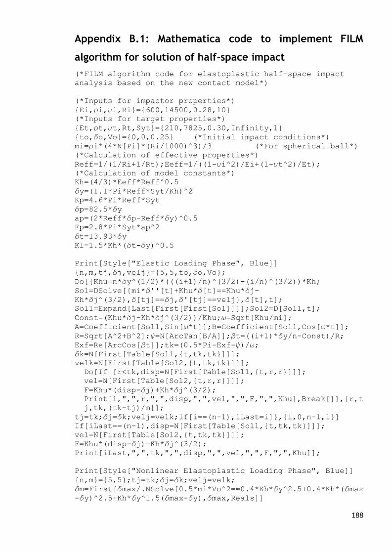
188

Appendix B.1: Mathematica code to implement FILM

algorithm for solution of half-space impact

(*FILM algorithm code for elastoplastic half-space impact

analysis based on the new contact model*)

(*Inputs for impactor properties*)

{Ei,i,i,Ri}={600,14500,0.28,10} (*Inputs for target properties*)

{Et,t,t,Rt,Syt}={210,7825,0.30,Infinity,1} {to,o,Vo}={0,0,0.25} (*Initial impact conditions*) mi=i*(4*N[Pi]*(Ri/1000)^3)/3 (*For spherical ball*) (*Calculation of effective properties*)

Reff=1/(1/Ri+1/Rt);Eeff=1/((1-i^2)/Ei+(1-t^2)/Et); (*Calculation of model constants*)

Kh=(4/3)*Eeff*Reff^0.5

y=(1.1*Pi*Reff*Syt/Kh)^2 Kp=4.6*Pi*Reff*Syt

p=82.5*y ap=(2*Reff*p-Reff*y)^0.5 Fp=2.8*Pi*Syt*ap^2

t=13.93*y Kl=1.5*Kh*(t-y)^0.5

Print[Style["Elastic Loading Phase", Blue]]

{n,m,tj,j,velj}={5,5,to,o,Vo}; Do[{Khu=n*y^(1/2)*(((i+1)/n)^(3/2)-(i/n)^(3/2))*Kh; Sol=DSolve[{mi*''[t]+Khu*[t]==Khu*j-Kh*j^(3/2),[tj]==j,'[tj]==velj},[t],t]; Sol1=Expand[Last[First[First[Sol]]]];Sol2=D[Sol1,t];

Const=(Khu*j-Kh*j^(3/2))/Khu;=Sqrt[Khu/mi]; A=Coefficient[Sol1,Sin[*t]];B=Coefficient[Sol1,Cos[*t]]; R=Sqrt[A^2+B^2];=N[ArcTan[B/A]];t=((i+1)*y/n-Const)/R; Exf=Re[ArcCos[t]];tk=(0.5*Pi-Exf-)/; k=N[First[Table[Sol1,{t,tk,tk}]]]; velk=N[First[Table[Sol2,{t,tk,tk}]]];

Do[If [r<tk,disp=N[First[Table[Sol1,{t,r,r}]]];

vel=N[First[Table[Sol2,{t,r,r}]]];

F=Khu*(disp-j)+Kh*j^(3/2); Print[i,",",r,",",disp,",",vel,",",F,",",Khu],Break[]],{r,t

j,tk,(tk-tj)/m}];

tj=tk;j=k;velj=velk;If[i==(n-1),iLast=i]},{i,0,n-1,1}] If[iLast==(n-1),disp=N[First[Table[Sol1,{t,tk,tk}]]];

vel=N[First[Table[Sol2,{t,tk,tk}]]];

F=Khu*(disp-j)+Kh*j^(3/2); Print[iLast,",",tk,",",disp,",",vel,",",F,",",Khu]];

Print[Style["Nonlinear Elastoplastic Loading Phase", Blue]]

{n,m}={5,5};tj=tk;j=k;velj=velk; m=First[max/.NSolve[0.5*mi*Vo^2==0.4*Kh*y^2.5+0.4*Kh*(max-y)^2.5+Kh*y^1.5(max-y),max,Reals]]

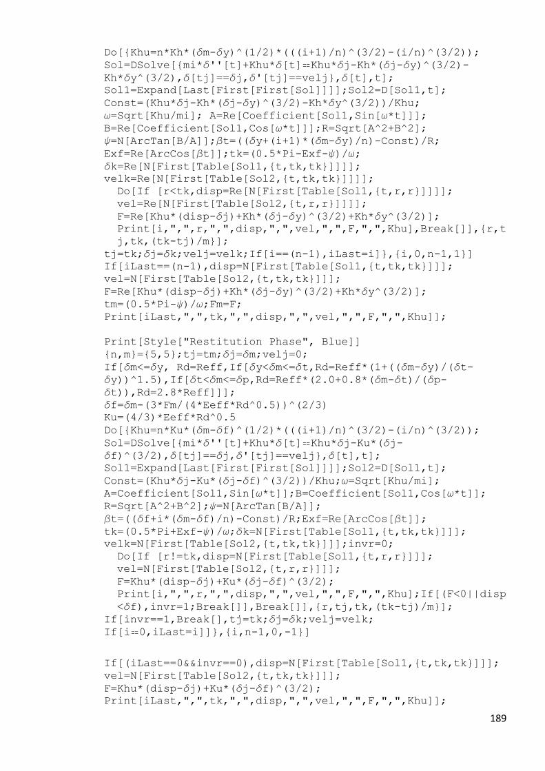
189

Do[{Khu=n*Kh*(m-y)^(1/2)*(((i+1)/n)^(3/2)-(i/n)^(3/2)); Sol=DSolve[{mi*''[t]+Khu*[t]Khu*j-Kh*(j-y)^(3/2)-Kh*y^(3/2),[tj]==j,'[tj]==velj},[t],t]; Sol1=Expand[Last[First[First[Sol]]]];Sol2=D[Sol1,t];

Const=(Khu*j-Kh*(j-y)^(3/2)-Kh*y^(3/2))/Khu; =Sqrt[Khu/mi]; A=Re[Coefficient[Sol1,Sin[*t]]]; B=Re[Coefficient[Sol1,Cos[*t]]];R=Sqrt[A^2+B^2]; =N[ArcTan[B/A]];t=((y+(i+1)*(m-y)/n)-Const)/R; Exf=Re[ArcCos[t]];tk=(0.5*Pi-Exf-)/; k=Re[N[First[Table[Sol1,{t,tk,tk}]]]]; velk=Re[N[First[Table[Sol2,{t,tk,tk}]]]];

Do[If [r<tk,disp=Re[N[First[Table[Sol1,{t,r,r}]]]];

vel=Re[N[First[Table[Sol2,{t,r,r}]]]];

F=Re[Khu*(disp-j)+Kh*(j-y)^(3/2)+Kh*y^(3/2)]; Print[i,",",r,",",disp,",",vel,",",F,",",Khu],Break[]],{r,t

j,tk,(tk-tj)/m}];

tj=tk;j=k;velj=velk;If[i==(n-1),iLast=i]},{i,0,n-1,1}] If[iLast==(n-1),disp=N[First[Table[Sol1,{t,tk,tk}]]];


F=Re[Khu*(disp-j)+Kh*(j-y)^(3/2)+Kh*y^(3/2)]; tm=(0.5*Pi-)/;Fm=F; Print[iLast,",",tk,",",disp,",",vel,",",F,",",Khu]];

Print[Style["Restitution Phase", Blue]]

{n,m}={5,5};tj=tm;j=m;velj=0; If[m<=y, Rd=Reff,If[y<m<=t,Rd=Reff*(1+((m-y)/(t-y))^1.5),If[t<m<=p,Rd=Reff*(2.0+0.8*(m-t)/(p-t)),Rd=2.8*Reff]]]; f=m-(3*Fm/(4*Eeff*Rd^0.5))^(2/3) Ku=(4/3)*Eeff*Rd^0.5

Do[{Khu=n*Ku*(m-f)^(1/2)*(((i+1)/n)^(3/2)-(i/n)^(3/2)); Sol=DSolve[{mi*''[t]+Khu*[t]Khu*j-Ku*(j-f)^(3/2),[tj]==j,'[tj]==velj},[t],t]; Sol1=Expand[Last[First[First[Sol]]]];Sol2=D[Sol1,t];

Const=(Khu*j-Ku*(j-f)^(3/2))/Khu;=Sqrt[Khu/mi]; A=Coefficient[Sol1,Sin[*t]];B=Coefficient[Sol1,Cos[*t]]; R=Sqrt[A^2+B^2];=N[ArcTan[B/A]]; t=((f+i*(m-f)/n)-Const)/R;Exf=Re[ArcCos[t]]; tk=(0.5*Pi+Exf-)/;k=N[First[Table[Sol1,{t,tk,tk}]]]; velk=N[First[Table[Sol2,{t,tk,tk}]]];invr=0;

Do[If [r!=tk,disp=N[First[Table[Sol1,{t,r,r}]]];


F=Khu*(disp-j)+Ku*(j-f)^(3/2); Print[i,",",r,",",disp,",",vel,",",F,",",Khu];If[(F<0||disp

<f),invr=1;Break[]],Break[]],{r,tj,tk,(tk-tj)/m}]; If[invr==1,Break[],tj=tk;j=k;velj=velk; If[i0,iLast=i]]},{i,n-1,0,-1}]

If[(iLast==0&&invr==0),disp=N[First[Table[Sol1,{t,tk,tk}]]];


F=Khu*(disp-j)+Ku*(j-f)^(3/2); Print[iLast,",",tk,",",disp,",",vel,",",F,",",Khu]];

190

Appendix B.2: Mathematica code to implement FILM

algorithm for infinite plate impact

(*FILM algorithm code for infinite plate impact analysis*)

(*Definition of units: bending stiffness - kNmm=Nm, contact

stiffness - kN/mm^1.5, density - kg/mm^2, velocity -

m/s=mm/ms, mass – kg, distance- mm*)

(*Inputs for impactor properties*)

{Ei,i,i,Ri}={210,7850,0.3,6.35} (*Inputs for target - orthotropic laminate ply properties*)

{D11,D12,D22,D66}={154.9,4.760,91.4,8.970}

{t,Rt,l,w,h}={4.132*10^-6,Infinity, 200,200,2.69} (*Other inputs*)

{mi,Vo}={8.3*10^-3,3} (*Calculation of effective properties*)

R=1/(1/Ri+1/Rt)

A=(D12+2*D66)/Sqrt[D11*D22] (*A is non-dimensionsal*)

Dteff=((A+1)/2)*Sqrt[D11*D22];Dp=Dteff;

Eeff=9.72 (*Given but can be calculated as Eeff=1/((1-

i)/Ei+1/Ez)*)

(*Calculation of model constants*)

Kh=(4/3)*Eeff*Sqrt[R] (*units - *)

{m,n,q,tj,j,velj}={10,50,70,0,0,3};maxcond=0; (*maxcond has an initial value of 0, which is set to 1 when

maximum condition is reached*)

(*Initial value of maximum indentation used is that of a

half-space*)

m=(5*mi*velj^2/(4*Kh))^(2/5) Print[Style["Loading Phase", Blue]]

Do[{Krs=n*m^(1/2)*(((i+1)/n)^(3/2)-(i/n)^(3/2))*Kh; rs=Krs/(8*Sqrt[Dp*t]);Prs=(Krs/mi)*j-(Kh/mi)*j^(3/2); Sol=DSolve[{''[t]+rs*'[t]+(Krs/mi)*[t]Prs,[tj]==j,'[tj]==velj},[t],t];Sol1=Last[First[First[Sol]]]; Sol2=D[Sol1,t];k=(i+1)*m/n;tk=t/.FindRoot[Sol1-k==0,{t,1.1*tj},MaxIterationsInfinity,AccuracyGoal3,PrecisionGoal8]; velk=N[First[Table[Sol2,{t,tk,tk}]]]; Do[If [r!=tk,disp=N[First[Table[Sol1,{t,r,r}]]];


F=Krs*(disp-j)+Kh*j^(3/2);velimp=vel+F/(8*Sqrt[Dp*t]); If[vel0.00001,tm=r;m1=N[First[Table[Sol1,{t,tm,tm}]]]; vm=N[First[Table[Sol2,{t,tm,tm}]]];

Fm=Krs*(m1-j)+Kh*j^(3/2); n=i;maxcond=1;Break[]],Break[]];

Print[i,",",r*10^3,",",disp*10^3,",",vel*10^2,",",velimp*10

^2,",",F*10^3,",",Krs];,{r,tj,tk,(tk-tj)/m}];

If[maxcond==1,tj=tm;j=m1;velj=vm;Break[]];tj=tk;j=k;velj=velk;},{i,0,n-1,1}]

191

Print[Style["Time at maximum indentation = ",

Red],Style[tm*10^3, Red]]

Print[Style["Maximum indentation = ", Red],Style[m1*10^3, Red]]

Print[Style["Relative velocity at maximum indentation = ",

Red],Style[vm*10^2, Red]]

Print[Style["Maximum Force = ", Red],Style[Fm*10^3, Red]]

n (*n is the discretisation where maximum condition occurs*)

(*n and m are reset based on the segment at which maximum condition is satisfied*)

Print[Style["Restitution Phase", Blue]]

endcond=0 ;(*endcond has an initial value of 0, which is set

to 1 when the end of the loading is reached*)

Do[{Krs=q*m1^(1/2)*(((i+1)/q)^(3/2)-(i/q)^(3/2))*Kh; rs=Krs/(8*Sqrt[Dp*t]);Prs=(Krs/mi)*j-(Kh/mi)*j^(3/2); Sol=DSolve[{''[t]+rs*'[t]+(Krs/mi)*[t]Prs,[tj]==j,'[tj]==velj},[t],t];Sol1=Last[First[First[Sol]]]; Sol2=D[Sol1,t];k=(i)*m1/q;tk=t/.FindRoot[Sol1-k==0,{t,1.1*tj},MaxIterationsInfinity,AccuracyGoal3,PrecisionGoal8];velk=N[First[Table[Sol2,{t,tk,tk}]]]; Do[If[r!=tk,disp=N[First[Table[Sol1,{t,r,r}]]];


F=Krs*(disp-j)+Kh*j^(3/2);velimp=vel+F/(8*Sqrt[Dp*t]); If[endcond==0,If[velimp0.00001,{te=r;de=N[First[Table[Sol1,{t,te,te}]]];ve=N[First[Table[Sol2,{t,te,te}]]];Fe=Krs*(de

-j)+Kh*j^(3/2);veimp=ve+Fe/(8*Sqrt[Dp*t]);endcond=1}]]; If[(F1.0E-8||disp1.0E-8),Break[]];,Break[]]; Print[i,",",r*10^3,",",disp*10^3,",",vel*10^2,",",velimp*10

^2,",",F*10^3,",",Krs];If[i==0&&r==tk-(tk-

tj)/m,disp=N[First[Table[Sol1,{t,tk,tk}]]];


F=Krs*(disp-j)+Kh*j^(3/2);velimp=vel+F/(8*Sqrt[Dp*t]); Print[i,",",tk*10^3,",",disp*10^3,",",vel*10^2,",",velimp*1

0^2,",",F*10^3,",",Krs];];,{r,tj,tk,(tk-tj)/m}];

tj=tk;j=k;velj=velk;},{i,q-1,0,-1}]

Print[Style["Time at end of loading = ", Red],Style[te*10^3,

Red]]

Print[Style["Indentation at end of loading = ",

Red],Style[de*10^3, Red]]

Print[Style["Relative velocity at end of loading = ",

Red],Style[ve*10^2, Red]]

Print[Style["Impactor velocity at end of loading = ",

Red],Style[veimp*10^2, Red]]

Print[Style["Force at end of loading = ", Red],Style[Fe*10^3,

Red]]

ClearAll

192

Appendix B.3: Mathematica code to solve the impact

model of the trimorph plate

(*Code for the solution of the trimorph plate impact model*) {a,b,1,2,3,1,2,3,E1,E2,E3,den1,den2,den3}={0.1,0.1,0.001,0.001,0.008,0.3,0.44,0.33,64000000000,1100000000,7000000000

0,7600,1770,2700};{mp,V0,Ei,i,Ri,Rp,Sy1,Sy2,Sy3,}={1.0,0.30,210000000000,0.3,0.01,Infinity,0.250,0.050,0.320,0};

h=1+2+3; (*Total thickness of the plate*) den=(den1*1+den2*2+den3*3)/h (*Density of the plate*)

(*Bending stiffnesses*)

D111=(E1/(1-1^2))*(1^3-1.5*h*1*(1-h/2)); D112=(E2/(1-2^2))*(2^3+3*2*(1-h/2)*(1+2-h/2)); D113=(E3/(1-3^2))*(3^3+3*3*(1+2-h/2)*(1+2+3-h/2)); D11=(D111+D112+D113)/3;

D121=(1*E1/(1-1^2))*(1^3-1.5*h*1*(1-h/2)); D122=(2*E2/(1-2^2))*(2^3+3*2*(1-h/2)*(1+2-h/2)); D123=(3*E3/(1-3^2))*(3^3+3*3*(1+2-h/2)*(1+2+3-h/2)); D12=(D121+D122+D123)/3;

D661=(E1/(1+1))*(1^3-1.5*h*1*(1-h/2)); D662=(E2/(1+2))*(2^3+3*2*(1-h/2)*(1+2-h/2)); D663=(E3/(1+3))*(3^3+3*3*(1+2-h/2)*(1+2+3-h/2)); D66=(D661+D662+D663)/6;

(*This section of the code calculates all the constants in

the ODE, solves the ODE, and plots the result to aid visual

assessment of the response*)

Ep=h/(1/E1+2/E2+3/E3);p=(1*1+2*2+3*3)/h; Syt=h/(1/Sy1+2/Sy2+3/Sy3) Eeff=Ei*Ep/(Ep*(1-i^2)+Ei*(1-p^2)); Reff=1/(1/Ri+1/Rp);Kh=((4/3)*Eeff*Reff^0.5)/(1000^2.5)

y=(1.1*Pi*Reff*1000*Syt/Kh)^2 (*Indentation at yield*) velstress=Sqrt[Ep/den];tstress=h/velstress

(*Code for obtaining the set of ODEs and initial conditions

necessary for the solution of the ELASTIC impact response

based on the number of participating modes specified.*)

{m,n}={5,5}; (*Participating modes*)

z=0;a=0;Kb=0; (*Initialisation of number of participating modes and approximate plate displacement*)

Do[

Do[z=z+1;Dbar=((22/7)^4)*(i^4*D11/(a^4)+j^4*D11/(b^4)+2*i^2

*j^2*(D12+2*D66)/(a^2*b^2))/(den*h);K=(1-)*Dbar/1000000; a=a+StringReplacePart["z[t]",ToString[z],{2,2}]*Sin[i*Pi/2]*Sin[j*Pi/2];

Fcoeff=(4*Kh/(den*a*b*h))*Sin[i*Pi/2]*Sin[j*Pi/2];

eqn=""<>ToString[z]<>"''[t]"+K*""<>ToString[z]<>"[t]=="<>ToString[Fcoeff*dis]<>"^1.5";If[z1,modevars=""<>ToString[z],modevars=modevars<>","<>ToString[z]];

193

If[z1,modeics=""<>ToString[z]<>"[0]==0,"<>ToString[z]<>"'[0]==0",modeics=modeics<>","<>ToString[z]<>"[0]==0,"<>ToString[z]<>"'[0]==0"];

If[z1,modeeqns=ToString[eqn],modeeqns=modeeqns<>", "<>ToString[eqn]];,{j,1,n,2}]

,{i,1,m,2}];

reldis=b[t]-a (*reldis is the Indentation. Since a is a string at this stage reldis should be converted to expression

before using it in a computation.*);

modeeqns1=StringReplace[modeeqns,"dis""("<>ToString[reldis]<>")"];pvars=StringSplit[StringReplace[modevars<>",b[t]",",""[t],"],","]; (*Set of response variables solved for*)

(*Solution of the elastic impact response*)

td={};

ndSol1=NDSolve[{ToExpression[StringSplit["b''[t]+"<>ToString[(Kh/mp)]<>"*("<>ToString[reldis]<>")^1.5==0,"<>modeeqns1,","

]],ToExpression[StringSplit[modeics<>",b[0]==0,b'[0]==V0",","]],WhenEvent[Re[b[t]-#1]0,AppendTo[td,t]]&[a/.str_StringToExpression[str]]},ToExpression[StringSplit[modevars<>",b",","]],{t,0,10},MaxStepsInfinity]; tde=First[td] (*time duration of elastic impact*)

dmaxlist={} (*Initialization of list of all turning

points on the indentation curve during elastic impact*);

NDSolve[{ToExpression[StringSplit["b''[t]+"<>ToString[(Kh/mp)]<>"*("<>ToString[reldis]<>")^1.5==0,"<>modeeqns1,","]],ToEx

pression[StringSplit[modeics<>",b[0]==0,b'[0]==V0",","]],WhenEvent[Re[b'[t]-#1]0,AppendTo[dmaxlist,{t,Re[b[t]-#2]}]]&[D[a/.str_StringToExpression[str],t],a/.str_StringToExpression[str]]},ToExpression[StringSplit[modevars<>",b",","]],{t,0,tde},MaxStepsInfinity];

tme=First[SortBy[dmaxlist,Last][[-1]]] (*Time at maximum

indentation of elastic loading response*)

dme=Last[SortBy[dmaxlist,Last][[-1]]] (*Indentation maximum

of elastic loading response*)

If [dmey,{(*Plot of impact force, dispacements and indentation responses for elastic impact*)

Print[Plot[{(ToExpression[ToString[Kh]<>"*("<>"b[t]-("<>ToString[a]<>"))^1.5"])/.ndSol1},{t,0,10},AxesLabel{Style["Time [ms]",Medium,Bold],Style["Force

[kN]",Medium,Bold]},PlotRangeAutomatic]]; Print[Plot[{b[t]/.ndSol1,ToExpression["("<>ToString[a]<>")"]/.ndSol1,ToExpression["b[t]-("<>ToString[a]<>")"]/.ndSol1},{t,0,tde},AxesLabel{Style["Time [ms]",Medium,Bold],Style["Disp.

[mm]",Medium,Bold]},PlotStyle{Directive[Black,Dashing[Tiny]],Directive[Black,Dashing[Small]],Directive[Black]}

,PlotLegends{"Impactor disp.","Plate disp. "<>ToString[(m+1)*(n+1)/4]<>" modes approx.","Indentation

194

"<>ToString[(m+1)*(n+1)/4]<>" modes

approx."},PlotRangeAutomatic]]; Print[Plot[{b'[t]/.ndSol1,ToExpression["("<>StringReplace[ToString[a],"[t]""'[t]"]<>")"]/.ndSol1,(b'[t]-ToExpression["("<>StringReplace[ToString[a],"[t]""'[t]"]<>")"])/.ndSol1},{t,0,tde},AxesLabel{Style["Time [ms]",Medium,Bold],Style["Vel.

[m/s]",Medium,Bold]},PlotStyle{Directive[Black],Directive[Black,Dashing[Small]],Directive[Black,Dashing[{0.06,0.02}]]},P

lotLegends{"Impactor vel.","Plate vel. "<>ToString[(m+1)*(n+1)/4]<>" modes approx.","Rel. vel.

"<>ToString[(m+1)*(n+1)/4]<>" modes

approx."},PlotRangeAutomatic]];Abort[]},

{tyList={};NDSolve[{ToExpression[StringSplit["b''[t]+"<>ToString[(Kh/mp)]<>"*("<>ToString[reldis]<>")^1.5==0,"<>modeeqns1

,","]],ToExpression[StringSplit[modeics<>",b[0]==0,b'[0]==V0",","]],WhenEvent[Re[b[t]-#1]-y0,AppendTo[tyList,t]]&[a/.str_StringToExpression[str]]},ToExpression[StringSplit[modevars<>",b",","]],{t,0,10},MaxStepsInfinity]; ty=First[tyList](*Time at yield point*);

Print[Table[Re[Evaluate[ToExpression["b[t]-("<>ToString[a]<>")"]/.ndSol1]],{t,ty,ty}]] (*Indentation obtained using ty*);


necessary for the solution of the ELASTOPLASTIC impact

response based on the number of participating modes*)

s=0;

Do[

Do[s=s+1;Dbar=((22/7)^4)*(i^4*D11/(a^4)+j^4*D11/(b^4)+2*i^2

*j^2*(D12+2*D66)/(a^2*b^2))/(den*h);K=(1-)*Dbar/1000000; Fcoeff=(4/(den*a*b*h))*Sin[i*Pi/2]*Sin[j*Pi/2];

eqn=""<>ToString[s]<>"''[t]"+K*""<>ToString[s]<>"[t]=="<>ToString[Fcoeff*Kh]<>"*("<>ToString[reldis-

y]<>")^1.5+"<>ToString[Fcoeff*Kh*y^1.5];

(*Determining the initial conditions of the elastoplastic

stage. When the numerical value of the initial condition is

small Mathematica automatically displays the number in

Standard form. This makes it difficult for string

operation. The Accounting form has been used to ensure that

the numerical values are in general form. A conditional

statement is used to account for negative sign with the

Accounting form.*)

If[s1,modeeqns2=ToString[eqn],modeeqns2=modeeqns2<>", "<>ToString[eqn]];If[s1,If[First[Re[Evaluate[ToExpression[""<>ToString[s]<>"[ty]"]/.ndSol1]]]<0,If[First[Re[Evaluate[ToExpression[""<>ToString[s]<>"'[ty]"]/.ndSol1]]]<0, modeics2=""<>ToString[s]<>"[ty]==-"<>ToString[AccountingForm[First[Re[Evaluate[ToExpression["

195

"<>ToString[s]<>"[ty]"]/.ndSol1]]]]]<>","<>ToString[s]<>"'[ty]==-

"<>ToString[AccountingForm[First[Re[Evaluate[ToExpression["

"<>ToString[s]<>"'[ty]"]/.ndSol1]]]]],modeics2=""<>ToString[s]<>"[ty]==-


"<>ToString[s]<>"[ty]"]/.ndSol1]]]]]<>","<>ToString[s]<>"'[ty]=="<>ToString[AccountingForm[First[Re[Evaluate[ToExpre

ssion[""<>ToString[s]<>"'[ty]"]/.ndSol1]]]]]],If[First[Re[Evaluate[ToExpression[""<>ToString[s]<>"'[ty]"]/.ndSol1]]]<0,modeics2=""<>ToString[s]<>"[ty]=="<>ToString[AccountingForm[First[Re[Evaluate[ToExpression[""<>ToString[s]<>"[ty]"]/.ndSol1]]]]]<>","<>ToString[s]<>"'[ty]==-"<>ToString[AccountingForm[First[Re[Evaluate[ToExpression["

"<>ToString[s]<>"'[ty]"]/.ndSol1]]]]],modeics2=""<>ToString[s]<>"[ty]=="<>ToString[AccountingForm[First[Re[Evaluate[

ToExpression[""<>ToString[s]<>"[ty]"]/.ndSol1]]]]]<>","<>ToString[s]<>"'[ty]=="<>ToString[AccountingForm[First[Re[Ev

aluate[ToExpression[""<>ToString[s]<>"'[ty]"]/.ndSol1]]]]]]],

If[First[Re[Evaluate[ToExpression[""<>ToString[s]<>"[ty]"]/.ndSol1]]]<0,If[First[Re[Evaluate[ToExpression[""<>ToString[s]<>"'[ty]"]/.ndSol1]]]<0,

modeics2=modeics2<>","<>ToString[s]<>"[ty]==-"<>ToString[AccountingForm[First[Re[Evaluate[ToExpression["

"<>ToString[s]<>"[ty]"]/.ndSol1]]]]]<>","<>ToString[s]<>"'[ty]==-


"<>ToString[s]<>"'[ty]"]/.ndSol1]]]]],modeics2=modeics2<>","<>ToString[s]<>"[ty]==-"<>ToString[AccountingForm[First[Re[Evaluate[ToExpression["

"<>ToString[s]<>"[ty]"]/.ndSol1]]]]]<>","<>ToString[s]<>"'[ty]=="<>ToString[AccountingForm[First[Re[Evaluate[ToExpre

ssion[""<>ToString[s]<>"'[ty]"]/.ndSol1]]]]]],If[First[Re[Evaluate[ToExpression[""<>ToString[s]<>"'[ty]"]/.ndSol1]]]<0,modeics2=modeics2<>","<>ToString[s]<>"[ty]=="<>ToString[AccountingForm[First[Re[Evaluate[ToExpression[""<>ToString[s]<>"[ty]"]/.ndSol1]]]]]<>","<>ToString[s]<>"'[ty]==-"<>ToString[AccountingForm[First[Re[Evaluate[ToExpression["

"<>ToString[s]<>"'[ty]"]/.ndSol1]]]]],modeics2=modeics2<>","<>ToString[s]<>"[ty]=="<>ToString[AccountingForm[First[Re[Evaluate[ToExpression[""<>ToString[s]<>"[ty]"]/.ndSol1]]]]]<>","<>ToString[s]<>"'[ty]=="<>ToString[AccountingForm[First[Re[Evaluate[ToExpression[""<>ToString[s]<>"'[ty]"]/.ndSol1]]]]]]]];,{j,1,n,2}]

,{i,1,m,2}];

(*Display the initial conditions of elastoplastic loading

response for checking*)

196

ToExpression[StringSplit[modeics2<>",b[ty]=="<>ToString[First[Re[Evaluate[b[ty]/.ndSol1]]]]<>",b'[ty]=="<>ToString[First[Re[Evaluate[b'[ty]/.ndSol1]]]],","]];

(*Solution of the elastoplastic impact response*)

dmax1list={};

If[First[Re[Evaluate[b'[ty]/.ndSol1]]]<0,ndSol2=NDSolve[{ToExpression[StringSplit["b''[t]+"<>ToString[(Kh/mp)]<>"*("<>ToString[reldis-

y]<>")^1.5+"<>ToString[(Kh/mp)*y^1.5]<>"==0,"<>modeeqns2,","]],ToExpression[StringSplit[modeics2<>",b[ty]=="<>ToString[First[Re[Evaluate[b[ty]/.ndSol1]]]]<>",b'[ty]==-"<>ToString[AccountingForm[First[Re[Evaluate[b'[ty]/.ndSol1]]]]],","]],WhenEvent[Re[b'[t]-#1]0,AppendTo[dmax1list,{t,Re[b[t]-#2]}]]&[D[a/.str_StringToExpression[str],t],a/.str_StringToExpression[str]]},ToExpression[StringSplit[modevars<>",b",","]],{t,ty,1.2*tde},MaxStepsInfinity],ndSol2=NDSolve[{ToExpression[StringSplit["b''[t]+"<>ToString[(Kh/mp)]<>"*("<>ToString[reldis-

y]<>")^1.5+"<>ToString[(Kh/mp)*y^1.5]<>"==0,"<>modeeqns2,","]],ToExpression[StringSplit[modeics2<>",b[ty]=="<>ToString[First[Re[Evaluate[b[ty]/.ndSol1]]]]<>",b'[ty]=="<>ToString[AccountingForm[First[Re[Evaluate[b'[ty]/.ndSol1]]]]],","]],WhenEvent[Re[b'[t]-#1]0,AppendTo[dmax1list,{t,Re[b[t]-#2]}]]&[D[a/.str_StringToExpression[str],t],a/.str_StringToExpression[str]]},ToExpression[StringSplit[modevars<>",b",","]],{t,ty,1.2*tde},MaxStepsInfinity]];

tm=First[SortBy[dmax1list,Last][[-1]]] (*Time at maximum

indentation of the elastoplastic loading response*);

dm=Last[SortBy[dmax1list,Last][[-1]]] (*Maximum

Indentation of elastoplastic loading response*);

Fm=First[First[Table[Re[Evaluate[(ToExpression[ToString[Kh]<>

"*("<>ToString[reldis-

y]<>")^1.5+"<>ToString[Kh*y^1.5]])/.ndSol2]],{t,tm,tm}]]] (*Maximum force of elastoplastic loading response*);

teList={};

NDSolve[{ToExpression[StringSplit["b''[t]+"<>ToString[(Kh/mp)]<>"*("<>ToString[reldis-

y]<>")^1.5+"<>ToString[(Kh/mp)*y^1.5]<>"==0,"<>modeeqns2,","]],ToExpression[StringSplit[modeics2<>",b[ty]=="<>ToString[First[Re[Evaluate[b[ty]/.ndSol1]]]]<>",b'[ty]=="<>ToString[AccountingForm[First[Re[Evaluate[b'[ty]/.ndSol1]]]]],","]],WhenEvent[Re[b'[t]]0,AppendTo[teList,t]]},ToExpression[StringSplit[modevars<>",b",","]],{t,ty,tde},MaxStepsInfinity];

te=First[teList] (*Time at the end of the loading phase

i.e. when the velocity of the projectile is zero*);

Ve=Table[Re[Evaluate[b'[t]/.ndSol2]],{t,te,te}] (*Velocity of impactor at the end of the loading phase.*);

197

de=First[First[Table[Re[Evaluate[(b[t]-ToExpression["("<>ToString[a]<>")"])/.ndSol2]],{t,te,te}]]] (*indentation at the end of the loading phase*);


necessary for the solution of the ELASTIC UNLOADING impact

response based on the number of participating modes*)

x=0;

F1=First[First[Table[Re[Evaluate[(ToExpression[ToString[Kh]<>

"*("<>"b[t]-("<>ToString[a]<>"))^1.5"])/.ndSol1]],{t,te,te}]]] (*Elastic Impact force at te*);

Fe=First[First[Table[Re[Evaluate[(ToExpression[ToString[Kh]<>

"*("<>ToString[reldis-

y]<>")^1.5+"<>ToString[Kh*y^1.5]])/.ndSol2]],{t,te,te}]]] (*Impact force at the end of elastoplastic loading*);

If[de<=y,Rd=Reff,Rd=Reff*(1+((de-y)/(12.93*y))^1.5)] (*Deformed effective radius*);

df=de-(3*Fe/(4*(Eeff*10^-9)*(1000*Rd)^0.5))^(2/3) (*Permanent

indentation at the end of the impact event*);

Ku=((4/3)*Eeff*Rd^0.5)/(1000^2.5);

Do[

Do[x=x+1;Dbar=((22/7)^4)*(i^4*D11/(a^4)+j^4*D11/(b^4)+2*i^2

*j^2*(D12+2*D66)/(a^2*b^2))/(den*h);K=(1-)*Dbar/1000000; Fcoeff=(4/(den*a*b*h))*Sin[i*Pi/2]*Sin[j*Pi/2];

eqn=""<>ToString[x]<>"''[t]"+K*""<>ToString[x]<>"[t]=="<>ToString[Fcoeff*Ku]<>"*("<>ToString[reldis-

df]<>")"<>"^1.5";

If[x1,modeeqns3=ToString[eqn],modeeqns3=modeeqns3<>", "<>ToString[eqn]];If[x1,If[First[Re[Evaluate[ToExpression[""<>ToString[x]<>"[te]"]/.ndSol2]]]<0,If[First[Re[Evaluate[ToExpression[""<>ToString[x]<>"'[te]"]/.ndSol2]]]<0,modeics3=""<>ToString[x]<>"[te]==-"<>ToString[AccountingForm[First[Re[Evaluate[ToExpression["

"<>ToString[x]<>"[te]"]/.ndSol2]]]]]<>","<>ToString[x]<>"'[te]==-


"<>ToString[x]<>"'[te]"]/.ndSol2]]]]],modeics3=""<>ToString[x]<>"[te]==-


"<>ToString[x]<>"[te]"]/.ndSol2]]]]]<>","<>ToString[x]<>"'[te]=="<>ToString[AccountingForm[First[Re[Evaluate[ToExpre

ssion[""<>ToString[x]<>"'[te]"]/.ndSol2]]]]]],If[First[Re[Evaluate[ToExpression[""<>ToString[x]<>"'[te]"]/.ndSol2]]]<0,modeics3=""<>ToString[x]<>"[te]=="<>ToString[AccountingForm[First[Re[Evaluate[ToExpression[""<>ToString[x]<>"[te]"]/.ndSol2]]]]]<>","<>ToString[x]<>"'[te]==-"<>ToString[AccountingForm[First[Re[Evaluate[ToExpression["

"<>ToString[x]<>"'[te]"]/.ndSol2]]]]],modeics3=""<>ToString[x]<>"[te]=="<>ToString[AccountingForm[First[Re[Evaluate[

ToExpression[""<>ToString[x]<>"[te]"]/.ndSol2]]]]]<>","<>ToString[x]<>"'[te]=="<>ToString[AccountingForm[First[Re[Ev

198

aluate[ToExpression[""<>ToString[x]<>"'[te]"]/.ndSol2]]]]]]],

If[First[Re[Evaluate[ToExpression[""<>ToString[x]<>"[te]"]/.ndSol2]]]<0,If[First[Re[Evaluate[ToExpression[""<>ToString[x]<>"'[te]"]/.ndSol2]]]<0,

modeics3=modeics3<>","<>ToString[x]<>"[te]==-"<>ToString[AccountingForm[First[Re[Evaluate[ToExpression["

"<>ToString[x]<>"[te]"]/.ndSol2]]]]]<>","<>ToString[x]<>"'[te]==-


"<>ToString[x]<>"'[te]"]/.ndSol2]]]]],modeics3=modeics3<>","<>ToString[x]<>"[te]==-"<>ToString[AccountingForm[First[Re[Evaluate[ToExpression["

"<>ToString[x]<>"[te]"]/.ndSol2]]]]]<>","<>ToString[x]<>"'[te]=="<>ToString[AccountingForm[First[Re[Evaluate[ToExpre

ssion[""<>ToString[x]<>"'[te]"]/.ndSol2]]]]]],If[First[Re[Evaluate[ToExpression[""<>ToString[x]<>"'[te]"]/.ndSol2]]]<0,modeics3=modeics3<>","<>ToString[x]<>"[te]=="<>ToString[AccountingForm[First[Re[Evaluate[ToExpression[""<>ToString[x]<>"[te]"]/.ndSol2]]]]]<>","<>ToString[x]<>"'[te]==-"<>ToString[AccountingForm[First[Re[Evaluate[ToExpression["

"<>ToString[x]<>"'[te]"]/.ndSol2]]]]],modeics3=modeics3<>","<>ToString[x]<>"[te]=="<>ToString[AccountingForm[First[Re[Evaluate[ToExpression[""<>ToString[x]<>"[te]"]/.ndSol2]]]]]<>","<>ToString[x]<>"'[te]=="<>ToString[AccountingForm[First[Re[Evaluate[ToExpression[""<>ToString[x]<>"'[te]"]/.ndSol2]]]]]]]];,{j,1,n,2}]

,{i,1,m,2}];

(*Display the initial conditions for the unloading impact

response*)

StringSplit[modeics3<>",b[te]=="<>ToString[AccountingForm[First[Re[Evaluate[b[te]/.ndSol2]]]]]<>",b'[te]=="<>ToString[AccountingForm[First[Re[Evaluate[b'[te]/.ndSol2]]]]],","];

ToExpression[StringSplit[modeics3<>",b[te]=="<>ToString[AccountingForm[First[Re[Evaluate[b[te]/.ndSol2]]]]]<>",b'[te]==-

"<>ToString[AccountingForm[First[Re[Evaluate[b'[te]/.ndSol2]]]]],","]];

(*Solution of the unloading impact response*)

If[First[Re[Evaluate[b'[te]/.ndSol2]]]<0,ndSol3=NDSolve[{ToExpression[StringSplit["b''[t]+"<>ToString[(Ku/mp)]<>"*("<>ToString[reldis-

df]<>")^1.5"<>"==0,"<>modeeqns3,","]],ToExpression[StringSpli

t[modeics3<>",b[te]=="<>ToString[AccountingForm[First[Re[Evaluate[b[te]/.ndSol2]]]]]<>",b'[te]==-"<>ToString[AccountingForm[First[Re[Evaluate[b'[te]/.ndSol2]]]]],","]]},ToExpression[StringSplit[modevars<>",b",","]],{t,te,1.5*tde},MaxStepsInfinity],ndSol3=NDSolve[{ToExpression

199

[StringSplit["b''[t]+"<>ToString[(Ku/mp)]<>"*("<>ToString[reldis-


t[modeics3<>",b[te]=="<>ToString[AccountingForm[First[Re[Evaluate[b[te]/.ndSol2]]]]]<>",b'[te]=="<>ToString[AccountingForm[First[Re[Evaluate[b'[te]/.ndSol2]]]]],","]]},ToExpression[StringSplit[modevars<>",b",","]],{t,te,1.5*tde},MaxStepsInfinity]];

tueList={};

NDSolve[{ToExpression[StringSplit["b''[t]+"<>ToString[(Ku/mp)]<>"*("<>ToString[reldis-


t[modeics3<>",b[te]=="<>ToString[AccountingForm[First[Re[Evaluate[b[te]/.ndSol2]]]]]<>",b'[te]=="<>ToString[AccountingForm[First[Re[Evaluate[b'[te]/.ndSol2]]]]],","]],WhenEvent[Re[b[t]-#1]-df0,AppendTo[tueList,t]]&[a/.str_StringToExpression[str]]},ToExpression[StringSplit[modevars<>",b",","]],{t,te,1.5*tde},MaxStepsInfinity];Print[tueList];tue1=First[tueList]; tue=t/.FindRoot[Re[Evaluate[(ToExpression[ToString[reldis-

df]])/.ndSol3]]0,{t,1.*tde}];

(*Print[Plot[Piecewise[{{Re[(ToExpression[ToString[Kh]<>"*("<

>"b[t]-("<>ToString[a]<>"))^1.5"])/.ndSol1],0tty},{Re[(ToExpression[ToString[Ky]<>"*("<>ToString[reldis-

y]<>")+"<>ToString[Kh*y^1.5]])/.ndSol2],tytte},{Re[(ToExpression[ToString[Ku]<>"*("<>ToString[reldis-

df]<>")"<>"^1.5"])/.ndSol3],tettue}}],{t,0,tue}]];*)

(*Displacement history plots for elastic impact*)

Print[Plot[{b[t]/.ndSol1,ToExpression["("<>ToString[a]<>")"]/.ndSol1,ToExpression["b[t]-("<>ToString[a]<>")"]/.ndSol1},{t,0,10},AxesLabel{Style["Time [ms]",Medium,Bold],Style["Disp.

[mm]",Medium,Bold]},GridLinesAutomatic, PlotStyle{Directive[Black,Dashing[Tiny]],Directive[Black,Dashing[Small]],Directive[Black]} ,PlotLegends{"Impactor disp.","Plate disp. "<>ToString[(m+1)*(n+1)/4]<>" modes

approx.","Indentation "<>ToString[(m+1)*(n+1)/4]<>" modes

approx."},PlotRangeAutomatic]];

(*Force history plot combining the different loading and

unloading stages of the impact*)

Print[Show[Plot[Re[(ToExpression[ToString[Kh]<>"*("<>"b[t]-("<>ToString[a]<>"))^1.5"])/.ndSol1],{t,0,ty},PlotStyleBlue],Plot[Re[(ToExpression[ToString[Kh]<>"*("<>ToString[reldis-

y]<>")^1.5+"<>ToString[Kh*y^1.5]])/.ndSol2],{t,ty,te},PlotStyleRed],Plot[Re[(ToExpression[ToString[Ku]<>"*("<>ToString[reldis-

df]<>")"<>"^1.5"])/.ndSol3],{t,te,tue},PlotStyleDarker[Blac

200

k]],PlotRange{{0,tue},Automatic},AxesLabel{Style["Time [ms]",Medium,Bold],Style["Force [kN]",Medium,Bold]}]];

(*Displacement history plots combining the different loading

and unloading stages of the impact*)

Print[Show[Plot[{b[t]/.ndSol1,ToExpression["("<>ToString[a]<>")"]/.ndSol1,ToExpression["b[t]-("<>ToString[a]<>")"]/.ndSol1},{t,0,ty},PlotStyle{Directive[Blue,Dashing[Tiny]],Directive[Blue,Dashing[Medium]],Directi

ve[Blue]}],Plot[{b[t]/.ndSol2,ToExpression["("<>ToString[a]<>")"]/.ndSol2,ToExpression["b[t]-("<>ToString[a]<>")"]/.ndSol2},{t,ty,te},PlotStyle{Directive[Red,Dashing[Tiny]],Directive[Red,Dashing[Medium]],Directiv

e[Red]}],Plot[{b[t]/.ndSol3,ToExpression["("<>ToString[a]<>")"]/.ndSol3,ToExpression["b[t]-("<>ToString[a]<>")"]/.ndSol3},{t,te,tue},PlotStyle{Directive[Darker[Black],Dashing[Tiny]],Directive[Darker[Black],Dash

ing[Medium]],Directive[Darker[Black]]}],PlotRange{{0,tue},Automatic},AxesLabel{Style["Time [ms]",Medium,Bold],Style["Disp. [mm]",Medium,Bold]}]];

(*Velocity history plots combining the different loading and

unloading stages of the impact*)

Print[Show[Plot[{b'[t]/.ndSol1,ToExpression["("<>StringReplace[ToString[a],"[t]""'[t]"]<>")"]/.ndSol1,(b'[t]-ToExpression["("<>StringReplace[ToString[a],"[t]""'[t]"]<>")"])/.ndSol1},{t,0,ty},PlotStyle{Directive[Blue,Dashing[Tiny]],Directive[Blue,Dashing[Medium]],Directive[Blue]}],Plot[{

b'[t]/.ndSol2,ToExpression["("<>StringReplace[ToString[a],"[t]""'[t]"]<>")"]/.ndSol2,(b'[t]-ToExpression["("<>StringReplace[ToString[a],"[t]""'[t]"]<>")"])/.ndSol2},{t,ty,te},PlotStyle{Directive[Red,Dashing[Tiny]],Directive[Red,Dashing[Medium]],Directive[Red]}],Plot[{b'[t]/.ndSol3,ToExpression["("<>StringReplace[ToString[a],"[t]""'[t]"]<>")"]/.ndSol3,(b'[t]-ToExpression["("<>StringReplace[ToString[a],"[t]""'[t]"]<>")"])/.ndSol3},{t,te,tue},PlotStyle{Directive[Darker[Black],Dashing[Tiny]],Directive[Darker[Black],Dashing[Medium]],Dire

ctive[Darker[Black]]}],PlotRange{{0,tue},Automatic},AxesLabel{Style["Time [ms]",Medium,Bold],Style["Vel. [m/s]",Medium,Bold]}]];

Print["ty = ",ty,", te = ",te,", tm = ",tm,", tue = ",tue,",

td = ",tde, ", df = ",df, ", Fe = ",Fe, ", de = ",de, ", dm =

",dm, ", Fm = ",Fm];}]

(*Obtaining data points from the solutions*)

If[dme>y,{Print["Elastic Impact response"];Do[Print[t," , ",First[Re[(ToExpression[ToString[Kh]<>"*("<>"b[t]-("<>ToString[a]<>"))^1.5"])/.ndSol1]]," , ",First[Re[ToExpression["b[t]-("<>ToString[a]<>")"]/.ndSol1]]," ,

201

",First[Re[ToExpression["("<>ToString[a]<>")"]/.ndSol1]]," , ",First[Re[b[t]/.ndSol1]]],{t,0,tde,tde/40}]; Print["Elastic loading"]

Do[Print[t," ,

",First[Re[(ToExpression[ToString[Kh]<>"*("<>"b[t]-("<>ToString[a]<>"))^1.5"])/.ndSol1]]," , ",First[Re[ToExpression["b[t]-("<>ToString[a]<>")"]/.ndSol1]]," , ",First[Re[ToExpression["("<>ToString[a]<>")"]/.ndSol1]]," , ",First[Re[b[t]/.ndSol1]]],{t,0,ty,ty/20}] Print["Elastoplastic loading"]

Do[Print[t," ,

",First[Re[(ToExpression[ToString[Kh]<>"*("<>ToString[reldis-

y]<>")^1.5+"<>ToString[Kh*y^1.5]])/.ndSol2]]," , ",First[Re[ToExpression["b[t]-("<>ToString[a]<>")"]/.ndSol2]]," , ",First[Re[ToExpression["("<>ToString[a]<>")"]/.ndSol2]]," , ",First[Re[b[t]/.ndSol2]]],{t,ty,te,(te-ty)/20}] Print["Elastic unloading"]

Do[Print[t," ,

",First[Re[(ToExpression[ToString[Ku]<>"*("<>ToString[reldis-

df]<>")"<>"^1.5"])/.ndSol3]]," ,

",First[Re[ToExpression["b[t]-("<>ToString[a]<>")"]/.ndSol3]]," , ",First[Re[ToExpression["("<>ToString[a]<>")"]/.ndSol3]]," , ",First[Re[b[t]/.ndSol3]]],{t,te,tue,(tue-te)/20}]},{Print["Elastic Impact response"];

Do[Print[t," ,

",First[Re[(ToExpression[ToString[Kh]<>"*("<>"b[t]-("<>ToString[a]<>"))^1.5"])/.ndSol1]]," ,

",First[Re[ToExpression["b[t]-("<>ToString[a]<>")"]/.ndSol1]]," ,

",First[Re[ToExpression["("<>ToString[a]<>")"]/.ndSol1]]," , ",First[Re[b[t]/.ndSol1]]],{t,0,tde,tde/40}]}]

202

REFERENCES

Abramovich, H. (1998): Deflection Control of Laminated Composite Beams with

Piezoceramic Layers - Closed Form Solutions, Composites Structures, 43, 217 –

231.

Abrate, S. (1998): Impact on Composite Structures, Cambridge University Press,

Cambridge.

Abrate, S. (2001): Modeling of Impacts on Composite Structures, Computers and

Structures, 51, pp 129 – 138.

Abrate, S. (2011): Impact Dynamics, In: Abrate, S. (ed) Impact Engineering of

Composite Structures, SpingerWien, New York.

Alcalá, J., Giannakopoulos, A.E., Suresh, S. (1998): Continuous Measurements of

Load Penetration Curves with Spherical Microindenters and the Estimation of

Mechanical Properties, Journal of Materials Research, 13, pp 1390–1400.

Anderson, T.A. (2005): An Investigation of SDOF Models for Large Mass Impact on

Sandwich Composites, Composites: Part B, 36, pp 135 – 142.

Angioni, S.L., Meo, M., Foreman, A. (2011): Impact Damage Resistance and

Damage Suppression Properties of Shape Memory Alloys in Hybrid Composites – A

Review, Smart Materials and Structures, 20, 013001.

Auricchio, F. and Sacco, E. (2003): Refined First-Order Shear Deformation Theory

Models for Composite Laminates, Journal of Applied Mechanics, 70, pp 381 –

390.

Bartier, O., Hernot, X., Mauvoisin, G., (2010): Theoretical and experimental

analysis of contact radius for spherical indentation, Mechanics of Materials, 42,

pp 640–656.

Bert, C.W. and Chen, T.L.C. (1978): Effect of Shear Deformation on Vibration of

Antisymmetric Angle-Ply Laminated Rectangular Plate, International Journal of

Solids and Structures, 14, pp 465 – 473.

Bicho, E., Mallet, P., Schoner, G. (2000): Target Representation on an

Autonomous Vehicle with Low-level Sensors, International Journal of Robotics

Research, 19 (5), pp 424 – 447.

Big-Alabo, A. and Cartmell, M.P. (2011): Vibration Analysis of a Trimorph Plate

for Optimised Damage Mitigation, Journal of Theoretical and Applied Mechanics,

49 (3), pp 641 – 664.

203

Big-Alabo, A. and Cartmell, M.P. (2012): Vibration Analysis of a Trimorph Plate

as a Precursor Model for Smart Automotive Bodywork, Journal of Physics:

Conference Series, 382 (012012).

Big-Alabo, A., Harrison P., Cartmell, M.P. (2014a): Elastoplastic Half-space

Impact Analysis Using a Novel Contact Model that Accounts for Post-yield Effects,

Proceedings of the 9th International Conference on Structural Dynamics,

EURODYN, Porto, 30 June – 2 July.

Big-Alabo, A., Harrison P., Cartmell, M.P. (2014b): Algorithm for the solution of

elastoplastic half-space impact: Force-Indentation Linearisation Method, Proc.

IMechE, Part C: Journal of Mechanical Engineering Sciences, Early Online

Publication, DOI: 10.1177/0954406214541431.

Big-Alabo, A., Harrison, P., Cartmell, M.P. (2015a): Contact Model for

Elastoplastic Analysis of Half-space Indentation by a Spherical Impactor,

Computers and Structures, 151, pp 20 – 29.

Big-Alabo, A., Harrison, P., Cartmell, M.P. (2015b): Preliminary Investigations of

the Low-Velocity Impact Response of a Smart Trimorph Plate for Active Damage

Mitigation, 5th Thematic Conference on Computational Methods in Structural

Dynamics and Earthquake Engineering, COMPDYN, Crete Island, Greece, 25 – 27

May, 2015.

Brake, M.R. (2012): An Analytical Elastic-Perfectly Plastic Contact Model,

International Journal of Solids and Structures, 49, pp 3129 – 3141.

Cairns, D.S. (1991): A Simple, Elasto-Plastic Contact Law for Composites, Journal

of Reinforced Plastics and Composites, 10, pp 423 – 433.

Carrera, E. (2004): On the Use of the Murakami’s Zig-Zag Function in the

Modelling of Layered Plates and Shells, Computers and Structures, 82, pp 541 –

554.

Carvalho, A. and Guedes Soares, C. (1996): Dynamic Response of Rectangular

Plates of Composite Materials Subjected to Impact Loads, Composite Structures,

34, pp 55 – 63.

Chai, G.B. and Zhu, S. (2011): A Review of Low-Velocity Impact on Sandwich

Structures, Proc. IMechE, Part L: Journal of Materials Design and Applications,

225, pp 207 – 230.

Chopra, I. (2002): Review of State of Art of Smart Structures and Integrated

Systems, AIAA Journal, 40 (11), pp 2145 – 2187.

Christoforou, A.P. and Swanson, S.R. (1991): Analysis of Impact Response in

Composite Plates, International Journal of Solids and Structures, 27 (2), pp 161

– 170.

204

Christoforou, A.P. and Yigit, A.S. (1995): Transient Response of a Composite

Beam Subject to Elastic-Plastic Impact, Composite Engineering, 5 (5), pp 459 –

470.

Christoforou, A.P. and Yigit, A.S. (1998a): Characterisation of Impact in

Composite Plates, Composite Structures, 43, pp 15 – 24.

Christoforou, A.P. and Yigit, A.S. (1998b): Effect of Flexibility on Low Velocity

Impact Response, Journal of Sound and Vibration, 217 (3), pp 563 – 578.

Corbett, G.G., Reid, S.R., Johnson, W. (1996): Impact Loading of Plates and

Shells by Free-flying Projectiles: A Review, International Journal of Impact

Engineering, 18 (2), pp 141 – 230.

Dharmarajan, S. and McCutchen, H. (Jr) (1973): Shear Coefficient for

Orthotropic Beams, Journal of Composite Materials, 7, pp 530 – 535.

Donadon et al, (2002): Stiffening Effects on the Natural Frequencies of

Laminated Plates with Piezoelectric Actuators, Composites: Part B, 33, pp 335 –

342.

Edery-Azulay, L. and Abramovich, H. (2006): Active Damping of Piezo-composite

Beams, Composites Structures, 74, 458 – 466.

Emile, G. and Matthew, H. (2003): The Assessment of Novel Materials and

Processes for the Impact Tolerant Design of Stiffened Composite Aerospace

Structures, Composites: Part A, 34, pp 151 – 161.

Foo, C.C., Seah, L.K., Chai, G.B. (2011): A Modified Energy-Balance to Predict

Low-Velocity Impact Response for Sandwich Composites, Computers and

Structures, Vol. 93, pp 1385 – 1393.

Ganilova, O.A. and Cartmell, M.P. (2010): An Analytical Model for the Vibration

of a Composite Plate Containing an Embedded Periodic Shape Memory Alloy

Structure, Composites Structures, Vol. 92, pp 39 – 47.

Ghugal, Y.M. and Shimpi, R.P. (2002): A Review of Refined Shear Deformation

Theories of Isotropic and Anisotropic Laminated Plates, Journal of Reinforced

Plastics and Composites, 21 (9), pp 775 – 813.

Goldsmith, W. (2001): Impact: The Theory and Physical Behaviour of Colliding

Solids, Dover Publications, New York.

Grunenfelder, L.K., Suksangpanya, N., Salinas, C., Milliron, G., Yaraghi, N.,

Herrera, S., Evans-Lutterodt, K., Nutt, S.R., Zavattieri, P., Kisailus, D. (2014):

Bio-inspired Impact-resistant Composites, Acta Biomaterialia, 10 (9), pp 3997 –

4008.

205

Hardy, C., Baronet, C.N., Tordion, G.V. (1971): The Elasto-Plastic Indentation of

a Half-Space by a Rigid Sphere, International Journal for Numerical Methods in

Engineering, 3, pp 451-462.

Hernandes, J.A., Almeida, S.F.M., Nabarrete, A. (2000): Stiffening Effects on the

Free Vibration Behavior of Composite Plates with PZT Actuators, Composite

Structures, 49, pp 55 – 63.

Hill, R., Storakers, B., Zdunek, A.B. (1989): A Theoretical Study of Brinell

Hardness Test, Proceedings of Royal Society London A, 423, pp 301 – 330.

Hunter, S.C. (1957): Energy Absorbed by Elastic Waves During Impact, Journal of

Mechanics and Physics of Solids, 5, pp 162 – 171.

Hutchings, I.M. (1979): Energy Absorbed by Elastic Wave During Plastic Impact,

Journal of Physics D: Applied Physics, 12, pp 1819 – 1824.

Israr, A. (2008): Vibration Analysis of Cracked Aluminium Plates, PhD Thesis,

Department of Mechanical Engineering, University of Glasgow, UK.

Jackson, R.L. and Green, I. (2005): A Finite Element Study of Elasto-Plastic

Hemispherical Contact Against a Rigid Flat, Journal of Tribology, 127, pp 343 –

354.

Jackson, R.L., Green, I., Marghitu, D.B. (2009): Predicting the Coefficient of

Restitution of Impacting Elastic-Perfectly Plastic Spheres, Nonlinear Dynamics,

60 (3), pp 217 – 229.

Johnson, K.L. (1985): Contact Mechanics, Cambridge University Press,

Cambridge.

Jones, R.M. (1999): Mechanics of Composite Materials, 2nd Edition, Taylor and

Francis, Philadelphia.

Kamiya R., Cheeseman, B.A., Popper, P., Chou, T.W. (2000): Some Recent

Advances in the Fabrication and Design Three-dimensional Textile Preforms: A

Review, Composites Science and Technology, 60, pp 33 – 47.

Karas, K. (1939): Platten unter seitchem stoss, Ingenieur Archiv, 10, pp 237-250.

Kazanci, Z. and Mecitoğlu, Z. (2008): Nonlinear dynamic behavior of simply

supported laminated composite plates subjected to blast load, Journal of Sound

and Vibration, 317, pp 883 – 897.

Khalili, M.R., Malekzadeh, K., Mittal, R.K. (2007c): Effect of Physical and

Geometrical Parameters on the Transverse Low-Velocity Impact Response of

Sandwich Panels with a Transversely Flexible Core, Composite Structures, 77, pp

430 – 443.

206

Khalili, S.M.R., Shokuhfar, A., Ghasemi, F.A. (2007d): Effect of Smart Stiffening

Procedure on Low-velocity Impact Response of Smart Structures, Journal of

Materials Processing Technology, 190, pp 142 – 152.

Khalili, S.M.R., Shokuhfar, A., Ghasemi, F.A., Malekzadeh, K. (2007a): Dynamic

Response of Smart Hybrid Composite Plate Subjected to Low-Velocity Impact,

Journal of Composite Materials, 41 (19), pp 2347 – 2370.

Khalili, S.M.R., Shokuhfar, A., Malekzadeh, K., Ghasemi, F.A. (2007b): Low-

Velocity Impact Response of Active Thin-walled Hybrid Composite Structures

Embedded with SMA Wires, Thin-walled Structures, 45, pp 799 – 808.

Kharaz, A.H. and Gorham, D.A. (2000): A Study of Coefficient of Restitution in

Elastic-Plastic Impact, Philosophical Magazine Letters, 80 (8), pp 549 – 559.

Larson, R.A. and Palazotto, A.N. (2009): Property Estimation in FGM Plates

Subject to Low-Velocity Impact Loading, Journal of Mechanics of Materials and

Structures, 4 (7-8), pp 1429 – 1451.

Lau, K., Ling, H., Zhou, L. (2004): Low-velocity Impact on Shape Memory Alloy

Stitched Composite Plates, Smart Materials and Structures, 13, pp 364 – 370.

Lazarus, K.B. (1989): Induced Strain Actuation of Composite Plates, SM Thesis,

Aero. and Astro. Dept., MIT Cambridge USA.

Lee, C.K. (1999): Theory of Laminated Piezoelectric Plates for the Design of

Distributed Sensors/Actuators. Part I: Governing Equations and Reciprocal

Relationships, Journal of Acoustical Society of America, 87 (3), pp 1144 – 1158.

Leissa, A.W. (1969): Vibration of Plates, NASA SP-160, U.S. Government Printing

Office.

Li, L.Y., Thornton, C., Wu, C.Y. (2000): Impact Behaviour of Elastoplastic

Spheres with a Rigid Wall, Proc. IMechE, Part C: Journal of Mechanical

Engineering Science, 214, pp 1107 – 1114.

Li, L.Y., Wu, C.Y., Thornton, C. (2002): A theoretical model for the contact of

elastoplastic bodies, Proc. IMechE, Part C: Journal of Mechanical Engineering

Science, 216, pp 421 – 431.

Li, N. and Mirza, S. (1995): Vibration of Antisymmetric Angle-Ply Laminated

Plates Including Transverse Shear Deformation, Mechanics of Composite

Materials and Structures, 2 (2), pp 163 – 175.

Liew, K. M., Kitipornchai, S., Wang, C. M., Xiang, Y (1998): Vibration of Mindlin

Plates: Programming the P-Version Ritz Method, 1st Edition, Elsevier,

Amsterdam.

Liew, K.M., He, X.Q., Tan, M.J., Lim, H.K. (2004): Dynamic Analysis of

Laminated Composite Plates with Piezoelectric Sensor/Actuator Patches using

207

the FSDT Mesh-free Method, International Journal of Mechanical Sciences, 46,

pp 411 – 431.

Lifshitz, J.M. and Kolsky, H. (1964): Some Experiments on Anelastic Rebound,

Journal of Mechanics and Physics of Solids, pp 12, 35 – 43.

Lin, J. and Nien, M.H. (2007): Adaptive Modeling and Shape Control of Laminated

Plates using Piezoelectric Actuators, Journal of Material Processing Technology,

189, pp 231 – 236.

Madabhusi-Raman, P. and Daralos, J.F. (1996): Static Shear Correction Factor for

Laminated Composite Rectangular Beams, Composites: Part B, 27, pp 285 – 293.

Majeed, M.A., Yigit, A.S., Christoforou, A.P. (2012): Elastoplastic

Contact/Impact of Rigidly Supported Composites, Composites: Part B, 43, pp

1244 – 1251.

Manoach, E. and Trendifilova, I. (2008): Large amplitude vibrations and damage

detection of rectangular plates, Journal of Sound and Vibration, 315, pp 591 –

606.

Mitchell, J.A. and Reddy, J.N. (1995): A Refined Hybrid Plate Theory for

Composite Laminates with Piezoelectric Laminae, International Journal of Solids

and Structures, 32 (6), pp 2345 – 2367.

Moita, J. M. S., Correia, I. F.P., Soares, C. M. M., Soares, C. A. M. (2004): Active

Control of Adaptive Laminated Structures with Bonded Piezoelectric Sensors and

Actuators, Computers and Structures, 82, pp 1349 – 1358.

Mok, C.H. and Duffy, J. (1965): The Dynamic Stress-Strain Relation of Metals as

Determined from Impact Test with a Hard Ball, International Journal of

Mechanical Sciences, 7, pp 355 – 371.

Mouritz, A.P. and Cox, M.K. (2010): A Mechanistic Interpretation of the

Comparative In-plane Mechanical Properties of 3D Woven, Stitched and Pinned

Composites, Composites: Part A, 41, pp 709 – 728.

Mouritz, A.P., Bannister, M.K., Falzon, P.J., Leong, K.H. (1999): Review of

Applications for Advanced Three-dimensional Fibre Textile Composites,

Composites: Part A, 30, pp 1445 – 1461.

Mujica, F. (2014): Scalable Electronics Driving Autonomous Vehicle Technologies,

Texas Instruments Inc., http://www.ti.com/lit/wp/sszy010a/sszy010a.pdf,

Accessed: 5 December 2014.

Nguyen, Q. and Tong, L. (2004): Shape Control of Smart Composite Plate with

Non-rectangular Piezoelectric Actuators, Composites Structures, 66, pp 207 –

214.

208

Nosier, A., Kapania, R.K., Reddy, J.N. (1994): Low-Velocity Impact of Laminated

Composite Plates Using a Layerwise Theory, Computational Mechanics, 13, pp

360 – 379.

Oguamanam, D.C.D., Almeida, S.F.M., Hansen, J.S. (1998): Stress Stiffening

Effects in Laminated Beams with Piezoelectric Actuators, Journal of Intellingent

Materials Systems and Structures, 9, pp 137 – 145.

Olsson, R. (1992): Impact Response of Orthotropic Composite Laminates

Predicted by a One-Parameter Differential Equation, AIAA Journal, 30 (6), pp

1587 – 1596.

Olsson, R. (2000): Mass Criterion for Wave Controlled Impact Response of

Composite Plates, Composites: Part A, 31, pp 879 – 887.

Olsson, R. (2001): Analytical Prediction of Large Mass Impact Damage in

Composite Laminates, Composites: Part A, 32, pp 1207 – 1215.

Olsson, R. (2002): Engineering Method for Prediction of Impact Response and

Damage in Sandwich Panels, Journal of Sandwich Structures and Materials, 4, pp

3 – 29.

Olsson, R. (2003): Closed Form Prediction of Peak Load and Delamination Onset

Under Small Mass Impact, Composite Structures, 59, pp 341 – 349.

Olsson, R., Donadon, M.V., Falzon, B.G. (2006): Delamination Threshold Load for

Dynamic Impact on Plates, International Journal of Solids and Structures, 43, pp

3124 – 3141.

Omidvar, B. (1998): Shear Coefficient in Orthotropic Thin-Walled Composite

Beams, Journal of Composites for Construction, 2 (1), pp 46 – 56.

Preumont, A. (2011): Vibration Control of Active Structures, 3rd Edition,

Springer-Verlag, Berlin.

Reddy, J.N. (1984): A Refined Non-Linear Theory of Plates with Transverse Shear

Deformation, International Journal of Solids and Structures, 20 (9-10), pp 881 –

896.

Reddy, J.N. (1999): On Laminated Composite Plates with Integrated Sensors and

Actuators, Engineering Structures, 21, pp 568 – 593.

Reddy, J.N. (2004): Mechanics of Laminated Composite Plates and Shells: Theory

and Analysis, 2nd Edition, CRC Press, Boca Raton.

Saravanos, D.A. and Christoforou, A.P. (2002): Impact Response of Adaptive

Piezoelectric Laminated Plates, AIAA Journal, 40 (10), pp 2087 – 2095.

Sears, J.E. (1908): On the Longitudinal Impact of Metal Rods with Rounded Ends,

Proceedings of the Cambridge Philosophical Society, 14, pp 257 – 286.

209

Shariyat, M. and Farzan, F. (2013): Nonlinear Eccentric Low-Velocity Impact

Analysis of Highly Prestressed FGM Rectangular Plate, Using a Refined Contact

Law, Archive of Applied Mechanics, 83, pp 623–641.

Shariyat, M. and Jafari, R. (2013): A Micromechanical Approach for Semi-

Analytical Low-Velocity Impact Analysis of Bidirectional Functionally Graded

Circular Plate Resting on an Elastic Foundation, Meccanica, 48, pp 2127 – 2148.

Shimpi, R.P., Patel, H.G., Arya, H. (2007): New Fisrt-Order Shear Deformation

Plate Theories, Journal of Applied Mechanics, 74, pp 523 – 533.

Staab, G.H. (1999): Laminar Composites, Butterworth Heinemann, Boston.

Stronge, W.J. (2000a): Impact Mechanics, Cambridge University Press,

Cambridge.

Stronge, W.J. (2000b): Contact Problems for Elasto-Plastic Impact in Multi-Body

Systems, In: Bernard Brogliato (Ed.) Impacts in Mechanical Systems: Analysis and

Modelling, Springer, Berlin.

Sun, C. T. and Yang, S. H. (1980): Contact Law and Impact Responses of

Laminated Composites, NASA Report – CR 159884.

Sutherland, L.S. and Guedes Soares, C. (2005): Contact indentation of marine

composites, Composites Structures, 70, pp 287– 294.

Szilard, R. (2004): Theory and Applications of Plate Analysis: Classical, Numerical

and Engineering Methods, John Wiley & Sons Inc., New Jersey.

Tabor, D. (1951): Hardness of Metals, Oxford University Press, London.

Teh, K.K and Haung, C.C (1979): Shear Deformation Coefficient for Generally

Orthotropic Beam, Fibre Science and Technology, 12, pp 73 – 80.

Thai, H.T. and Choi, D.H. (2013): A Simple First-Order Shear Deformation Theory

for Laminated Composite Plates, Composite Structures, 106, pp 754 – 763.

Thompson, S.P. and Loughlan, J. (1995): The Active Buckling Control of some

Composite Column Strips using Piezoceramic Actuators, Composite Structures,

32, pp 59 – 67.

Thornton, C. and Ning, Z. (1998): A Theoretical Model for Stick/Bounce

Behaviour of Adhesive Elastic-Plastic Spheres, Powder Technology, 99, pp 154 –

162.

Tillett, J.P.A. (1954): A Study of the Impact of Spheres on Plate, Proceedings of

the Physical Society: Section B, 67 (9), pp 677 – 688.

Timoshenko, S. and Woinowsky-krieger, S. (1959): Theory of Plates and Shells,

2nd Edition, McGraw-Hill, New York.

210

Timoshenko, S.P. (1913): Zur farge nach der wirkung eines Stosses auf einen

Balken, Z.A.M.P., 62, pp 198 – 209.

Turner, J.R. (1980): Contact on a Transversely Isotropic Half-space, or between

Two Transversely Isotropic Bodies, International Journal of Solids and

Structures, 16(5), pp 409 – 419.

Vinson, J.R. and Sierakowski, R.L. (2004) The Behaviour of Structures Composed

of Composite Materials, 2nd Edition, Kluwer Academic Publishers, New York.

Waisman, H. and Abramovich, H. (2002): Active Stiffening of Laminated

Composite Beams using Piezoelectric Actuators, Composites Structures, 58, pp

109 – 120.

Wittrick, W.H. (1987): Analytical, Three-Dimensional Elasticity Solutions to Some

Plate Problems, and Some Observations on Mindlin’s Plate Theory, International

Journal of Solids and Structures, 23 (4), pp 441 – 464.

Wolfram Research Inc. (2012): Mathematica Version 9.0, Wolfram Research Inc.,

Champaign, Illinois.

Wu, C., Li, L., Thornton, C. (2003): Rebound behaviour of spheres for plastic

impacts, International Journal of Impact Engineering, 28, pp 929 – 946.

Wu, C.Y., Li, L.Y., Thornton, C., (2005): Energy Dissipation During Normal

Impact of Elastic and Elastic-Plastic Spheres, International Journal of Impact

Engineering, 32, pp 593 – 604.

Wu, E. and Shyu, K. (1993): Response of Composite Laminates to Contact Loads

and Relationship to Low-Velocity Impact, Journal of Composite Materials, 27, pp

1443 – 1464.

Yigit, A.S. and Christoforou, A.P. (1994): On the Impact of a Spherical Indenter

and an Elastic-Plastic Isotropic Half-Space, Composite Engineering, 4 (11), pp

1143 – 1152.

Yigit, A.S. and Christoforou, A.P. (1995): Impact Dynamics of Composite Beams,

Composite Structures, 32, pp 187 – 195.

Yigit, A.S. and Christoforou, A.P. (2000): Control of Low-velocity Impact

Response on Composite Plates, Journal of Vibration and Control, 6, pp 429 –

447.

Zak, A.J. and Cartmell, M.P. (2000): Analytical Modelling of Shape Memory Alloys

and Flat Multilayered Composite Beams and Plates with Shape Memory Alloy

Wires, Technical Report (Grant number: GR/N06267/01), Department of

Mechanical Engineering, University of Glasgow, UK.

211

Zak, A.J., Cartmell, M.P. and Ostachowicz, W. (2003): Dynamics of Multilayered

Composite Plates with Shape Memory Alloy Wire, Journal of Applied Mechanics,

70, pp 313 – 327.

Zener, C. (1941): The Intrinsic Inelasticity of Large Plates, Physical Review, 59,

pp 669 – 673.

Zheng, D. and Binienda, W.K. (2007): Effect of Permanent Indentation on the

Delamination Threshold for Small Mass Impact on Plates, International Journal of

Solids and Structures, 44, pp 8143 – 8158.

Zhu, F.,Wang, Z., Lu, G., Nurick, G. (2010): Some Theoretical Considerations on

the Dynamic Response of Sandwich Structures Under Impulsive Loading,

International Journal of Impact Engineering, 37, pp 625 – 637.

Documents

Big-Alabo, Akuro (2015) Multilayered sensor -actuator ...theses.gla.ac.uk/6474/7/2015Big-Alabophd.pdf · Big-Alabo, Akuro (2015) Multilayered sensor -actuator plates for active mitigation