BIFURCATION ANALYSIS OF A MATHEMATICAL MODEL FOR

SIAM J. APPL. MATH. c© 2006 Society for Industrial and Applied MathematicsVol. 67, No. 1, pp. 24–45

BIFURCATION ANALYSIS OF A MATHEMATICAL MODEL FORMALARIA TRANSMISSION∗

NAKUL CHITNIS† , J. M. CUSHING‡ , AND J. M. HYMAN§

Abstract. We present an ordinary differential equation mathematical model for the spread ofmalaria in human and mosquito populations. Susceptible humans can be infected when they arebitten by an infectious mosquito. They then progress through the exposed, infectious, and recoveredclasses, before reentering the susceptible class. Susceptible mosquitoes can become infected whenthey bite infectious or recovered humans, and once infected they move through the exposed andinfectious classes. Both species follow a logistic population model, with humans having immigrationand disease-induced death. We define a reproductive number, R0, for the number of secondarycases that one infected individual will cause through the duration of the infectious period. We findthat the disease-free equilibrium is locally asymptotically stable when R0 < 1 and unstable whenR0 > 1. We prove the existence of at least one endemic equilibrium point for all R0 > 1. In theabsence of disease-induced death, we prove that the transcritical bifurcation at R0 = 1 is supercritical(forward). Numerical simulations show that for larger values of the disease-induced death rate, asubcritical (backward) bifurcation is possible at R0 = 1.

Key words. malaria, epidemic model, reproductive number, bifurcation theory, endemic equi-libria, disease-free equilibria

AMS subject classifications. Primary, 92D30; Secondary, 37N25

DOI. 10.1137/050638941

1. Introduction. Malaria is an infectious disease caused by the Plasmodiumparasite and transmitted between humans through the bite of the female Anophelesmosquito. An estimated 40% of the world’s population live in malaria endemic ar-eas. The disease kills about 1 to 3 million people a year, 75% of whom are Africanchildren. The incidence of malaria has been growing recently due to increasing para-site drug-resistance and mosquito insecticide-resistance. Therefore, it is important tounderstand the important parameters in the transmission of the disease and developeffective solution strategies for its prevention and control.

Mathematical modeling of malaria began in 1911 with Ross’s model [25], andmajor extensions are described in Macdonald’s 1957 book [20]. The first models weretwo-dimensional with one variable representing humans and the other representingmosquitoes. An important addition to the malaria models was the inclusion of ac-quired immunity proposed by Dietz, Molineaux, and Thomas [11]. Further work onacquired immunity in malaria has been conducted by Aron [2] and Bailey [5]. Ander-son and May [1], Aron and May [3], Koella [15] and Nedelman [21] have written somegood reviews on the mathematical modeling of malaria. Some recent papers have alsoincluded environmental effects [19], [27], and [28]; the spread of resistance to drugs

∗Received by the editors August 25, 2005; accepted for publication (in revised form) June 30, 2006;published electronically November 3, 2006. The authors thank the United States National ScienceFoundation for the following grants: NSF DMS-0414212 and NSF DMS-0210474. This research hasalso been supported under Department of Energy contract W-7405-ENG-36. Analysis of a similarmodel was published in the Ph.D. dissertation of the first author; see [7].

http://www.siam.org/journals/siap/67-1/63894.html†Corresponding author. Department of Public Health and Epidemiology, Swiss Tropical Institute,

Socinstrasse 57, P. O. Box, CH-4002 Basel, Switzerland ([email protected]).‡Department of Mathematics, University of Arizona, Tucson, AZ 85721 ([email protected].

edu).§Mathematical Modeling and Analysis (T-7), Los Alamos National Laboratory, Los Alamos, NM

87545 ([email protected]).

24

ANALYSIS OF A MATHEMATICAL MODEL FOR MALARIA 25

Fig. 1.1. Susceptible humans, Sh, can be infected when they are bitten by infectious mosquitoes.They then progress through the exposed, Eh, infectious, Ih, and recovered, Rh, classes, before re-entering the susceptible class. Susceptible mosquitoes, Sv, can become infected when they bite in-fectious or recovered humans. The infected mosquitoes then move through the exposed, Ev, and in-fectious, Iv, classes. Both species follow a logistic population model, with humans having additionalimmigration and disease-induced death. Birth, death, and migration into and out of the populationare not shown in the figure.

[4] and [16]; and the evolution of immunity [17].Recently, Ngwa and Shu [23] and Ngwa [22] proposed an ordinary differential

equation (ODE) compartmental model for the spread of malaria with a suscep-tible-exposed-infectious-recovered-susceptible (SEIRS) pattern for humans and asusceptible-exposed-infectious (SEI) pattern for mosquitoes. In a Ph.D. dissertation,Chitnis [7] analyzed a similar model for malaria transmission. In this paper we extendthe Chitnis model.

The new model (Figure 1.1) divides the human population into four classes: sus-ceptible, Sh; exposed, Eh; infectious, Ih; and recovered (immune), Rh. People enterthe susceptible class either through birth (at a constant per capita rate) or throughimmigration (at a constant rate). When an infectious mosquito bites a susceptiblehuman, there is some finite probability that the parasite (in the form of sporozoites)will be passed on to the human and that the person will move to the exposed class.The parasite then travels to the liver where it develops into its next life stage. Aftera certain period of time, the parasite (in the form of merozoites) enters the bloodstream, usually signaling the clinical onset of malaria. In our model, people from theexposed class enter the infectious class at a rate that is the reciprocal of the durationof the latent period. After some time, the infectious humans recover and move to therecovered class. The recovered humans have some immunity to the disease and donot get clinically ill, but they still harbor low levels of parasite in their blood streamsand can pass the infection to mosquitoes. After some period of time, they lose theirimmunity and return to the susceptible class. Humans leave the population througha density-dependent per capita emigration and natural death rate, and through a percapita disease-induced death rate.

We divide the mosquito population into three classes: susceptible, Sv; exposed,

26 NAKUL CHITNIS, J. M. CUSHING, AND J. M. HYMAN

Ev; and infectious, Iv. Female mosquitoes (we do not include male mosquitoes inour model because only female mosquitoes bite animals for blood meals) enter thesusceptible class through birth. The parasite (in the form of gametocytes) enters themosquito with some probability when the mosquito bites an infectious human or arecovered human (the probability of transmission of infection from a recovered humanis much lower than that from an infectious human), and the mosquito moves fromthe susceptible to the exposed class. After some period of time, dependent on theambient temperature and humidity, the parasite develops into sporozoites and entersthe mosquito’s salivary glands, and the mosquito moves from the exposed class tothe infectious class. The mosquito remains infectious for life. Mosquitoes leave thepopulation through a per capita density-dependent natural death rate.

The extension of the Ngwa and Shu model [23] includes human immigration,excludes direct human recovery from the infectious to the susceptible class, and gen-eralizes the mosquito biting rate so that it applies to wider ranges of populations.In [23], the total number of mosquito bites on humans depends only on the numberof mosquitoes, while in our model, the total number of bites depends on both thehuman and mosquito population sizes. Human migration is present throughout theworld and plays a large role in the epidemiology of diseases, including malaria. Inmany parts of the developing world, there is rapid urbanization as many people leaverural areas and migrate to cities in search of employment. We include this move-ment as a constant immigration rate into the susceptible class. We do not includeimmigration of infectious humans, as we assume that most people who are sick willnot travel. We also exclude the movement of exposed humans because, given theshort time of the exposed stage, the number of exposed people is small. We make thesimplifying assumption that there is no immigration of recovered humans. We alsoexclude the direct infectious-to-susceptible recovery that the model of Ngwa and Shu[23] contains. This is a realistic simplifying assumption because most people showsome period of immunity before becoming susceptible again. As our model includesan exponential distribution of movement from the recovered to the susceptible class,it will include the quick return to susceptibility of some individuals. The model inChitnis [7] is the same as the model in this paper except for the mosquito biting rate,which is the same as in [23].

We first describe the mathematical model including the definition of a domainwhere the model is mathematically and epidemiologically well-posed. Next, we provethe existence and stability of a disease-free equilibrium point, define the reproductivenumber, and describe the existence and stability of the endemic equilibrium point(s).

2. Malaria model. The state variables (Table 2.1) and parameters (Table 2.2)for the malaria model (Figure 1.1) satisfy the equations in (2.1). All parameters

Table 2.1

The state variables for the malaria model (2.1).

Sh: Number of susceptible humansEh: Number of exposed humansIh: Number of infectious humansRh: Number of recovered (immune and asymptomatic, but slightly infectious) humansSv : Number of susceptible mosquitoesEv : Number of exposed mosquitoesIv : Number of infectious mosquitoesNh: Total human populationNv : Total mosquito population


Table 2.2

The parameters for the malaria model (2.1) and their dimensions.

Λh: Immigration rate of humans. Humans × Time−1.ψh: Per capita birth rate of humans. Time−1.ψv : Per capita birth rate of mosquitoes. Time−1.σv : Number of times one mosquito would want to bite humans per unit time, if humans were

freely available. This is a function of the mosquito’s gonotrophic cycle (the amount oftime a mosquito requires to produce eggs) and its anthropophilic rate (its preference forhuman blood). Time−1.

σh: The maximum number of mosquito bites a human can have per unit time. This is afunction of the human’s exposed surface area. Time−1.

βhv : Probability of transmission of infection from an infectious mosquito to a susceptiblehuman, given that a contact between the two occurs. Dimensionless.

βvh: Probability of transmission of infection from an infectious human to a susceptiblemosquito, given that a contact between the two occurs. Dimensionless.

βvh: Probability of transmission of infection from a recovered (asymptomatic carrier) humanto a susceptible mosquito, given that a contact between the two occurs. Dimensionless.

νh: Per capita rate of progression of humans from the exposed state to the infectious state.1/νh is the average duration of the latent period. Time−1.

νv : Per capita rate of progression of mosquitoes from the exposed state to the infectiousstate. 1/νv is the average duration of the latent period. Time−1.

γh: Per capita recovery rate for humans from the infectious state to the recovered state. 1/γhis the average duration of the infectious period. Time−1.

δh: Per capita disease-induced death rate for humans. Time−1.ρh: Per capita rate of loss of immunity for humans. 1/ρh is the average duration of the

immune period. Time−1.μ1h: Density-independent part of the death (and emigration) rate for humans. Time−1.μ2h: Density-dependent part of the death (and emigration) rate for humans. Humans−1 ×

Time−1.μ1v : Density-independent part of the death rate for mosquitoes. Time−1.μ2v : Density-dependent part of the death rate for mosquitoes. Mosquitoes−1 × Time−1.

are strictly positive with the exception of the disease-induced death rate, δh, whichis nonnegative. The mosquito birth rate is greater than the density-independentmosquito death rate, ψv > μ1v, ensuring that we have a stable positive mosquitopopulation.

dSh

dt= Λh + ψhNh + ρhRh − λh(t)Sh − fh(Nh)Sh,(2.1a)

dEh

dt= λh(t)Sh − νhEh − fh(Nh)Eh,(2.1b)

dIhdt

= νhEh − γhIh − fh(Nh)Ih − δhIh,(2.1c)

dRh

dt= γhIh − ρhRh − fh(Nh)Rh,(2.1d)

dSv

dt= ψvNv − λv(t)Sv − fv(Nv)Sv,(2.1e)

dEv

dt= λv(t)Sv − νvEv − fv(Nv)Ev,(2.1f)

dIvdt

= νvEv − fv(Nv)Iv,(2.1g)

where fh(Nh) = μ1h+μ2hNh is the per capita density-dependent death and emigrationrate for humans and fv(Nv) = μ1v +μ2vNv is the per capita density-dependent deathrate for mosquitoes. The total population sizes are Nh = Sh + Eh + Ih + Rh and


Nv = Sv + Ev + Iv, with

dNh

dt= Λh + ψhNh − fh(Nh)Nh − δhIh,(2.2a)

dNv

dt= ψvNv − fv(Nv)Nv,(2.2b)

and the infection rates are

λh = bh(Nh, Nv) · βhv ·IvNv

and λv = bv(Nh, Nv) ·(βvh · Ih

Nh+ βvh · Rh

Nh

).

(2.3)

We define the force of infection from mosquitoes to humans, λh, as the product of thenumber of mosquito bites that one human has per unit time, bh, the probability ofdisease transmission from the mosquito to the human, βhv, and the probability thatthe mosquito is infectious, Iv/Nv. We define the force of infection from humans tomosquitoes, λv, as the sum of the force of infection from infectious humans and fromrecovered humans. These are defined as the number of human bites one mosquitohas per unit time, bv; the probability of disease transmission from the human to themosquito, βvh and βvh; and the probability that the human is infectious or recovered,Ih/Nh and Rh/Nh. Here, we model the total number of mosquito bites on humans as

b = b(Nh, Nv) =σvNvσhNh

σvNv + σhNh=

σvσh

σv(Nv/Nh) + σhNv,(2.4)

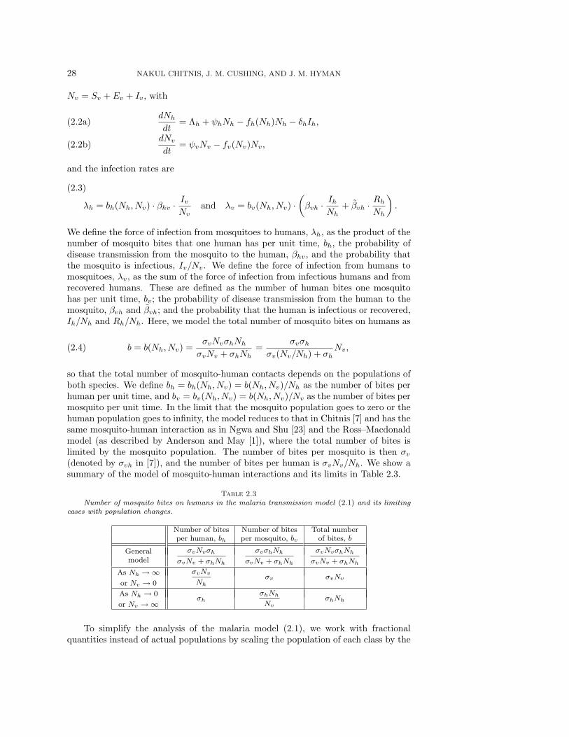
so that the total number of mosquito-human contacts depends on the populations ofboth species. We define bh = bh(Nh, Nv) = b(Nh, Nv)/Nh as the number of bites perhuman per unit time, and bv = bv(Nh, Nv) = b(Nh, Nv)/Nv as the number of bites permosquito per unit time. In the limit that the mosquito population goes to zero or thehuman population goes to infinity, the model reduces to that in Chitnis [7] and has thesame mosquito-human interaction as in Ngwa and Shu [23] and the Ross–Macdonaldmodel (as described by Anderson and May [1]), where the total number of bites islimited by the mosquito population. The number of bites per mosquito is then σv

(denoted by σvh in [7]), and the number of bites per human is σvNv/Nh. We show asummary of the model of mosquito-human interactions and its limits in Table 2.3.

Table 2.3

Number of mosquito bites on humans in the malaria transmission model (2.1) and its limitingcases with population changes.

Number of bites Number of bites Total numberper human, bh per mosquito, bv of bites, b

General σvNvσh

σvNv + σhNh

σvσhNh

σvNv + σhNh

σvNvσhNh

σvNv + σhNhmodel

As Nh → ∞ σvNv

Nhσv σvNv

or Nv → 0

As Nh → 0σh

σhNh

NvσhNh

or Nv → ∞

To simplify the analysis of the malaria model (2.1), we work with fractionalquantities instead of actual populations by scaling the population of each class by the


total species population. We let

eh =Eh

Nh, ih =

IhNh

, rh =Rh

Nh, ev =

Ev

Nv, and iv =

IvNv

,(2.5)

with

Sh = shNh = (1 − eh − ih − rh)Nh and Sv = svNv = (1 − ev − iv)Nv.(2.6)

Differentiating the scaling equations (2.5) and solving for the derivatives of the scaledvariables, we obtain

dehdt

=1

Nh

[dEh

dt− eh

dNh

dt

]and

devdt

=1

Nv

[dEv

dt− ev

dNv

dt

](2.7)

and so on for the other variables.This creates a new seven-dimensional system of equations with two dimensions for

the two total population variables, Nh and Nv, and five dimensions for the fractionalpopulation variables with disease, eh, ih, rh, ev, and iv:

dehdt

=

(σvσhNvβhvivσvNv + σhNh

)(1 − eh − ih − rh) −

(νh + ψh +

Λh

Nh

)eh + δhiheh,(2.8a)

dihdt

= νheh −(γh + δh + ψh +

Λh

Nh

)ih + δhi

2h,(2.8b)

drhdt

= γhih −(ρh + ψh +

Λh

Nh

)rh + δhihrh,(2.8c)

dNh

dt= Λh + ψhNh − (μ1h + μ2hNh)Nh − δhihNh,(2.8d)

devdt

=

(σvσhNh

σvNv + σhNh

)(βvhih + βvhrh

)(1 − ev − iv) − (νv + ψv)ev,(2.8e)

divdt

= νvev − ψviv,(2.8f)

dNv

dt= ψvNv − (μ1v + μ2vNv)Nv.(2.8g)

The model (2.8) is epidemiologically and mathematically well-posed in the domain

D =

⎧⎪⎪⎪⎪⎪⎪⎪⎪⎪⎪⎪⎪⎨⎪⎪⎪⎪⎪⎪⎪⎪⎪⎪⎪⎪⎩

⎛⎜⎜⎜⎜⎜⎜⎜⎜⎝

ehihrhNh

evivNv

⎞⎟⎟⎟⎟⎟⎟⎟⎟⎠

∈ R7

∣∣∣∣∣∣∣∣∣∣∣∣∣∣∣∣∣∣

eh ≥ 0,ih ≥ 0,rh ≥ 0,

eh + ih + rh ≤ 1,Nh > 0,ev ≥ 0,iv ≥ 0,

ev + iv ≤ 1,Nv > 0

⎫⎪⎪⎪⎪⎪⎪⎪⎪⎪⎪⎪⎪⎬⎪⎪⎪⎪⎪⎪⎪⎪⎪⎪⎪⎪⎭

.(2.9)

This domain, D, is valid epidemiologically as the fractional populations eh, ih, rh, ev,and iv are all nonnegative and have sums over their species type that are less than orequal to 1. The human and mosquito populations, Nh and Nv, are positive. We use thenotation f ′ to denote df/dt. We denote points in D by x = (eh, ih, rh, Nh, ev, iv, Nv).


Theorem 2.1. Assuming that the initial conditions lie in D, the system ofequations for the malaria model (2.8) has a unique solution that exists and remainsin D for all time t ≥ 0.

Proof. The right-hand side of (2.8) is continuous with continuous partial deriva-tives in D, so (2.8) has a unique solution. We now show that D is forward-invariant.We can see from (2.8) that if eh = 0, then e′h ≥ 0; if ih = 0, then i′h ≥ 0; if rh = 0,then r′h ≥ 0; if ev = 0, then e′v ≥ 0; and if iv = 0, then i′v ≥ 0. It is also true that ifeh + ih + rh = 1, then e′h + i′h + r′h < 0; and if ev + iv = 1, then e′v + i′v < 0. Finally,we note that if Nh = 0, then N ′

h > 0 and if Nv = 0, then N ′v = 0. If Nh > 0 at time

t = 0, then Nh > 0 for all t > 0. Similarly, if Nv > 0 at time t = 0, then Nv > 0 forall t > 0. Therefore, none of the orbits can leave D, and a unique solution exists forall time.

3. Disease-free equilibrium point and reproductive number.

3.1. Existence of the disease-free equilibrium point. Disease-free equi-librium points are steady-state solutions where there is no disease. We define the“diseased” classes as the human or mosquito populations that are either exposed,infectious, or recovered, that is, eh, ih, rh, ev, and iv. We denote the positive orthantin R

7 by R7+, and the boundary of R

7+ by ∂R

7+. The positive equilibrium human and

mosquito population values, in the absence of disease, for (2.8) are

N∗h =

(ψh − μ1h) +√

(ψh − μ1h)2 + 4μ2hΛh

2μ2hand N∗

v =ψv − μ1v

μ2v.(3.1)

Theorem 3.1. The malaria model (2.8) has exactly one equilibrium point, xdfe =(0, 0, 0, N∗

h , 0, 0, N∗v ), with no disease in the population (on D ∩ ∂R

7+).

Proof. We need to show that xdfe is an equilibrium point of (2.8) and that thereare no other equilibrium points on D ∩ ∂R

7+. Substituting xdfe into (2.8) shows all

derivatives equal to zero, so xdfe is an equilibrium point. We know from Lemma A.1that on D ∩ ∂R

7+, eh = ih = rh = ev = iv = 0. For ih = 0, the only equilibrium point

for Nh from (2.8d) is N∗h , and the only equilibrium point for Nv in D from (2.8g) is

N∗v . Thus, the only equilibrium point on D ∩ ∂R

7+ is xdfe.

3.2. Reproductive number. We use the next generation operator approachas described by Diekmann, Heesterbeek, and Metz in [10] to define the reproductivenumber, R0, as the number of secondary infections that one infectious individualwould create over the duration of the infectious period, provided that everyone else issusceptible. We define the next generation operator, K, which provides the number ofsecondary infections in humans and mosquitoes caused by one generation of infectioushumans and mosquitoes, as

K =

(0 Khv

Kvh 0

),(3.2)

where we use the following definitions:Khv: The number of humans that one mosquito infects through its infectious

lifetime, assuming all humans are susceptible.Kvh: The number of mosquitoes that one human infects through the duration of

the infectious period, assuming all mosquitoes are susceptible.Using the ideas of Hyman and Li [14], we define Khv and Kvh as products of

the probability of surviving till the infectious state, the number of contacts per unit


time, the probability of transmission per contact, and the duration of the infectiousperiod:

Khv =

(νv

νv + μ1v + μ2vN∗v

)· b∗v · βhv ·

(1

μ1v + μ2vN∗v

),(3.3a)

Kvh =

(νh

νh + μ1h + μ2hN∗h

)· b∗h · βvh ·

(1

γh + δh + μ1h + μ2hN∗h

)(3.3b)

+

(νh

νh + μ1h + μ2hN∗h

· γhγh + δh + μ1h + μ2hN∗

h

)

· b∗h · βvh ·(

1

ρh + μ1h + μ2hN∗h

).

In (3.3a), νv/(νv + μ1v + μ2vN∗v ) is the probability that a mosquito will survive the

exposed state to become infectious;1 b∗v = bv(N∗h , N

∗v ) is the number of contacts that

one mosquito has with humans per unit time; and 1/(μ1v + μ2vN∗v ) is the average

duration of the infectious lifetime of the mosquito. In (3.3b), the total number ofmosquitoes infected by one human is the sum of the new infections from the infectiousand from the recovered states of the human; νh/(νh +μ1h +μ2hN

∗h) is the probability

that a human will survive the exposed state to become infectious; γh/(γh +δh +μ1h +μ2hN

∗h) is the probability that the human will then survive the infectious state to

move to the recovered state; b∗h = bh(N∗h , N

∗v ) is the number of contacts that one

human has with mosquitoes per unit time; 1/(γh + δh + μ1h + μ2hN∗h) is the average

duration of the infectious period of a human; and 1/(ρh +μ1h +μ2hN∗h) is the average

duration of the recovered period of a human.We define R0 as the spectral radius of the next generation operator, K, i.e.,

R20 = KvhKhv. Then, R2

0 is the number of humans that one infectious human willinfect, through a generation of infections in mosquitoes, assuming that previously allother humans and mosquitoes were susceptible.

Definition 3.2. We define the reproductive number, R0, as

R0 =√KvhKhv,(3.4)

where Kvh and Khv are defined in (3.3).The original definition of the reproductive number of the Ross–Macdonald model

[1] and [3], and the Ngwa and Shu model [23], is equivalent to the square of this R0.They ([1], [3], and [23]) use the traditional definition of the reproductive number,which approximates the number of secondary infections in humans caused by oneinfected human, while the R0 in Definition 3.2 is consistent with the definition givenby the next generation operator approach [10], which approximates the number ofsecondary infections due to one infected individual (be it human or mosquito). Ourdefinition of R0 includes the generation of infections in mosquitoes, so is the squareroot of the original definition. The threshold condition for both definitions is thesame.

3.3. Stability of the disease-free equilibrium point.Theorem 3.3. The disease-free equilibrium point, xdfe, is locally asymptotically

stable if R0 < 1 and unstable if R0 > 1.The proof of this theorem is in the appendix section A.1.

1In defining periods of time and probabilities for R0, we use the original system of equations(2.1) and not the scaled equations (2.8). As the two models are equivalent, the reproductive numberis the same with either definition: μ1h + μ2hN

∗h = ψh + Λh/N

∗h and μ1v + μ2vN∗

v = ψv .


4. Endemic equilibrium points. Endemic equilibrium points are steady-statesolutions where the disease persists in the population (all state variables are positive).We use general bifurcation theory to prove the existence of at least one endemicequilibrium point for all R0 > 1. We prove that the transcritical bifurcation atR0 = 1 is supercritical (forward) when δh = 0 (there is no disease-induced death).However, numerical results show that the bifurcation can be subcritical (backward)for some positive values of δh, giving rise to endemic equilibria for R0 < 1.

We first rewrite the equilibrium equations for u = (eh, ev) in (2.8) as a nonlineareigenvalue problem in a Banach space:

u = G(ζ, u) = ζLu + h(ζ, u),(4.1)

where u ∈ Y ⊂ R2, with Euclidean norm ‖·‖; ζ ∈ Z ⊂ R is the bifurcation parameter;

L is a compact linear map on Y ; and h(ζ, u) is O(‖u‖2) uniformly on bounded ζintervals. We require that both Y and Z be open and bounded sets, and that Y containthe point 0. We define Z as the open and bounded set Z = {ζ ∈ R|−MZ < ζ < MZ}.This set is defined to include the characteristic values (reciprocals of eigenvalues) ofL, so there is minimum value that MZ can have, but MZ may be arbitrarily large.We use

ζ =σvσh

σvN∗v + σhN∗

h

(4.2)

for the bifurcation parameter. We also define Ω = Z × Y so that the pair (ζ, u) ∈ Ω.We denote the boundary of Ω by ∂Ω.

A corollary by Rabinowitz [24, Corollary 1.12] states that if ζ0 ∈ Z is a char-acteristic value of L of odd multiplicity, then there exists a continuum of nontrivialsolution-pairs (ζ, u) of (4.1) that intersects the trivial solution (that is, (ζ, 0) for any

ζ) at (ζ0, 0) and either meets ∂Ω or meets (ζ0, 0), where ζ0 is also a characteristic valueof L of odd multiplicity. We use this corollary to show that there exists a continuum ofsolution-pairs (ζ, u) ∈ Ω for the eigenvalue equation (4.1). To each of these solution-pairs there corresponds an equilibrium-pair (ζ, x∗). We define the equilibrium-pair,(ζ, x∗) ∈ Z × R

7, as the collection of a parameter value, ζ, and the correspondingequilibrium point, x∗, for that parameter value, of the malaria model (2.8).

Theorem 4.1. The model (2.8) has a continuum of equilibrium-pairs, (ζ, x∗) ∈Z ×R

7, that connects the point (ξ1, xdfe) to the hyperplane ζ = MZ in R×R7 on the

boundary of Z ×R7 for any MZ > ξ1, where x∗ is in the positive orthant of R

7. Hereξ1 = 1/

√AB, where A and B are defined in (A.19).

We show the proof of this theorem and related lemmas in appendix section A.2.Theorem 4.2. The transcritical bifurcation point at ζ = ξ1 corresponds to R0 =

1. For the set of ζ for which there exists an equilibrium-pair (ζ, x∗), the correspondingset of values for R0 includes, but is not necessarily identical to, the interval 1 < R0 <∞. Thus, there exists at least one endemic equilibrium point of the malaria model(2.8) for all R0 > 1.

Proof. Using the definition of ζ, (4.2), some algebraic manipulations of R0 (see(3.4)) produce

R0 = ζ√AB.(4.3)

Thus, R0 is linearly related to ζ, and when ζ = ξ1, R0 = 1. For any R0 > 1, (4.3)defines a corresponding ζ. We pick an MZ larger than this ζ. Then, Theorem 4.1


7 7.2 7.4 7.6 7.8 8

x 10−4

0

0.005

0.01

0.015

0.02

Bifurcation diagram showing endemic equilibrium points for two values of δ

h

δh =3.454e−4

δh =3.419e−5

Bifurcation Parameter: ζ

Fra

ctio

n of

exp

osed

hum

ans:

eh

Stable Equilibrium PointsUnstable Equilibrium Points

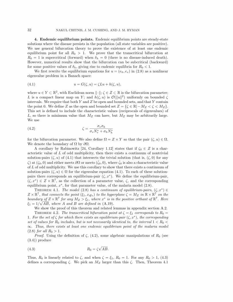
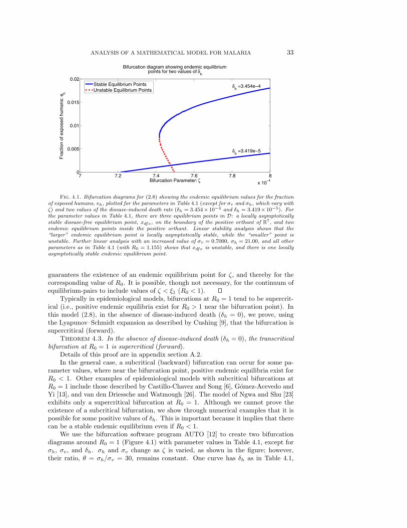
Fig. 4.1. Bifurcation diagrams for (2.8) showing the endemic equilibrium values for the fractionof exposed humans, eh, plotted for the parameters in Table 4.1 (except for σv and σh, which vary withζ) and two values of the disease-induced death rate (δh = 3.454× 10−4 and δh = 3.419× 10−5). Forthe parameter values in Table 4.1, there are three equilibrium points in D: a locally asymptoticallystable disease-free equilibrium point, xdfe, on the boundary of the positive orthant of R

7, and twoendemic equilibrium points inside the positive orthant. Linear stability analysis shows that the“larger” endemic equilibrium point is locally asymptotically stable, while the “smaller” point isunstable. Further linear analysis with an increased value of σv = 0.7000, σh = 21.00, and all otherparameters as in Table 4.1 (with R0 = 1.155) shows that xdfe is unstable, and there is one locallyasymptotically stable endemic equilibrium point.

guarantees the existence of an endemic equilibrium point for ζ, and thereby for thecorresponding value of R0. It is possible, though not necessary, for the continuum ofequilibrium-pairs to include values of ζ < ξ1 (R0 < 1).

Typically in epidemiological models, bifurcations at R0 = 1 tend to be supercrit-ical (i.e., positive endemic equilibria exist for R0 > 1 near the bifurcation point). Inthis model (2.8), in the absence of disease-induced death (δh = 0), we prove, usingthe Lyapunov–Schmidt expansion as described by Cushing [9], that the bifurcation issupercritical (forward).

Theorem 4.3. In the absence of disease-induced death (δh = 0), the transcriticalbifurcation at R0 = 1 is supercritical (forward).

Details of this proof are in appendix section A.2.In the general case, a subcritical (backward) bifurcation can occur for some pa-

rameter values, where near the bifurcation point, positive endemic equilibria exist forR0 < 1. Other examples of epidemiological models with subcritical bifurcations atR0 = 1 include those described by Castillo-Chavez and Song [6], Gomez-Acevedo andYi [13], and van den Driessche and Watmough [26]. The model of Ngwa and Shu [23]exhibits only a supercritical bifurcation at R0 = 1. Although we cannot prove theexistence of a subcritical bifurcation, we show through numerical examples that it ispossible for some positive values of δh. This is important because it implies that therecan be a stable endemic equilibrium even if R0 < 1.

We use the bifurcation software program AUTO [12] to create two bifurcationdiagrams around R0 = 1 (Figure 4.1) with parameter values in Table 4.1, except forσh, σv, and δh. σh and σv change as ζ is varied, as shown in the figure; however,their ratio, θ = σh/σv = 30, remains constant. One curve has δh as in Table 4.1,


Table 4.1

The parameter values for which there exist positive endemic equilibrium points when R0 < 1:R0 = 0.9898. The unit of time is days.

Λh = 3.285 × 10−2

ψh = 7.666 × 10−5 ψv = 0.4000βvh = 0.8333 βhv = 2.000 × 10−2

βvh = 8.333 × 10−2

σv = 0.6000 σh = 18.00νh = 8.333 × 10−2 νv = 0.1000γh = 3.704 × 10−3

δh = 3.454 × 10−4

ρh = 1.460 × 10−2

μ1h = 4.212 × 10−5 μ1v = 0.1429μ2h = 1.000 × 10−7 μ2v = 2.279 × 10−4

0 200 400 600 800 1000 1200 1400 1600 1800 200020

30

40

50

60

70

80Plot of infectious human population against time

Time (days)

Num

ber

of in

fect

ious

hum

ans:

I h

Initial Condition 1Initial Condition 2

Fig. 4.2. Solutions of the malaria model (2.1) with parameter values defined in Table 4.1 show-ing only the number of infectious humans, Ih, for two different initial conditions. The parameterscorrespond to R0 = 0.9898. Initial condition 1 is Sh = 400, Eh = 10, Ih = 30, Rh = 0, Sv = 1000,Ev = 100, and Iv = 50. Initial condition 2 is Sh = 700, Eh = 10, Ih = 30, Rh = 0, Sv = 1000,Ev = 100, and Iv = 50. The solution for initial condition 1 approaches the locally asymptoticallystable endemic equilibrium point, while the solution for initial condition 2 approaches the locallyasymptotically stable disease-free equilibrium point.

while the other has δh = 3.419 × 10−5. The curve with δh = 3.454 × 10−4 has bothunstable and stable endemic equilibrium points. There is a subcritical bifurcationat ζ = 7.494 × 10−4 (R0 = 1), and a saddle-node bifurcation at ζ = 7.417 × 10−4

(R0 = 0.9897). Thus a locally asymptotically stable endemic equilibrium is possiblefor values of R0 below 1. Further bifurcation analysis (not presented here) indicatesthat as ζ is increased to ζ = 50 (R0 = 66719), the size of the projection of theendemic equilibrium on the fractional infected groups increases monotonically, and theequilibrium point remains stable. For comparison we show the bifurcation diagramwith δh = 3.419 × 10−5. Here, we see only a stable branch of endemic equilibriumpoints. There is a supercritical bifurcation at ζ = 7.209 × 10−4 (R0 = 1). Thereare no endemic equilibrium points for R0 less than 1. As ζ is increased to ζ = 50(R0 = 69358), the size of the projection of the endemic equilibrium on the fractionalinfected groups increases monotonically, and the equilibrium point remains stable.

Figure 4.2 shows the infectious human population, for two different initial condi-


tions, of the solutions to the unscaled equations (2.1) for parameter values in Table 4.1with R0 < 1. One solution approaches the locally asymptotically stable endemic equi-librium point, while the other approaches the locally asymptotically stable disease-freeequilibrium point.

The parameter values in Table 4.1 are within the bounds of a realistically feasiblerange, except for the mosquito birth and death rates, ψv and μ1v, which have beenincreased to lower R0 below 1. More realistic values are ψv = 0.13 and μ1v = 0.033,which result in (with all other parameters as in Table 4.1) R0 = 1.6. More lists ofrealistic parameter values, and their references, can be found in [7] and [8]. δh =3.454 × 10−4 corresponds to a death rate of 12.62% of infectious humans per year.

5. Summary and conclusions. We analyzed an ordinary differential equa-tion model for the transmission of malaria, with four variables for humans and threevariables for mosquitoes. We showed that there exists a domain where the modelis epidemiologically and mathematically well-posed. We proved the existence of anequilibrium point with no disease, xdfe. We defined a reproductive number, R0, thatis epidemiologically accurate in that it provides the expected number of new infections(in mosquitoes or humans) from one infectious individual (human or mosquito) overthe duration of the infectious period, given that all other members of the populationare susceptible. We showed that if R0 < 1, then the disease-free equilibrium point,xdfe, is locally asymptotically stable, and if R0 > 1, then xdfe is unstable.

We also proved that an endemic equilibrium point exists for all R0 > 1 witha transcritical bifurcation at R0 = 1. The analysis and the numerical simulationsshowed that for δh = 0 (no disease-induced death), and for some small positive valuesof δh, there is a supercritical transcritical bifurcation at R0 = 1 with an exchange ofstability between the disease-free equilibrium and the endemic equilibrium. For largervalues of δh, there is a subcritical transcritical bifurcation at R0 = 1, with an exchangeof stability between the endemic equilibrium and the disease-free equilibrium; andthere is a saddle-node bifurcation at R0 = R∗

0 for some R∗0 < 1. Thus, for some

values of R0 < 1, there exist two endemic equilibrium points, the smaller of which isunstable, while the larger is locally asymptotically stable.

Although we cannot prove in general that the endemic equilibrium point is uniqueand stable for R0 > 1, numerical results for particular parameter sets suggest thatthere is a unique stable endemic equilibrium point for R0 > 1. Also, from Theorem 2.1it follows that all orbits of the malaria model (2.8) are bounded. Thus, if there wereno stable endemic equilibria in D, then there would exist a nonequilibrium attractor(such as a limit cycle or strange attractor), though for this model we have no evidencefor nonequilibrium attractors.

The possible existence of a subcritical bifurcation at R0 = 1 and a saddle-nodebifurcation at some R∗

0 < 1 can have implications for public health, when the epi-demiological parameters are close to those in Table 4.1. Simply reducing R0 to avalue below 1 is not always sufficient to eradicate the disease; it is now necessary toreduce R0 to a value less than R∗

0 to ensure that there are no endemic equilibria.The existence of a saddle-node bifurcation also implies that in some areas with en-demic malaria, it may be possible to significantly reduce prevalence or eradicate thedisease with small increases in control programs (a small reduction in R0 so that itis less than R∗

0). In some areas where malaria has been eradicated it is possible fora slight disruption, like a change in environmental or control variables or an influxof infectious humans or mosquitoes, to cause the disease to reestablish itself in thepopulation with a significant increase in disease prevalence (increasing R0 above R∗

0


or moving the system into the basin of attraction of the stable endemic equilibrium).As we have an explicit expression for R0, we can analytically evaluate its sensitiv-

ity to the different parameter values. We can also numerically evaluate the sensitivityof the endemic equilibrium to the parameter values. This allows us to determine therelative importance of the parameters to disease transmission and prevalence. As eachmalaria intervention strategy affects different parameters to different degrees, we canthus compare different control strategies for efficiency and effectiveness in reducingmalaria mortality and morbidity. This analysis, in the limiting case of the Chitnismodel [7] shows that malaria transmission is most sensitive to the mosquito bitingrate, and prevalence is most sensitive to the mosquito biting rate and the humanrecovery rate. The sensitivity analysis for the new model (2.8) is forthcoming [8].

We are extending the model to include the effects of the environment on thespread of malaria. Some parameters, such as the mosquito birth rate and the incuba-tion period in mosquitoes, depend on seasonal environmental factors such as rainfall,temperature, and humidity. We can include these effects by modeling these parame-ters as periodic functions of time. We would like to explore this periodically forcedmodel for features not seen in the autonomous model, including the modificationsto the definition of the reproductive number and the endemic states. This wouldprovide a more accurate picture of malaria transmission and prevalence than that ob-tained from models using parameter values that are averaged over the seasons. Otherplanned improvements to the model include the addition of age and spatial structure.

An ultimate goal is to validate this model by applying it to a particular malaria-endemic region of the world to compare the predicted endemic states with the preva-lence data.

Appendix. Lemmas and proofs of theorems.Lemma A.1. For all equilibrium points on D∩∂R

7+, eh = ih = rh = ev = iv = 0.

Proof. We need to show that for an equilibrium point in D, if any one of thediseased classes is zero, all the rest are also equal to zero. We show, by setting theright-hand side of (2.8) equal to 0, that if any one of eh, ih, rh, ev, or iv is equal to 0,then eh = ih = rh = ev = iv = 0. For i′h = 0, eh = 0 if and only if ih = 0.2 Similarly,for r′h = 0, ih = 0 if and only if rh = 0. Thus, if eh = 0, ih = 0, or rh = 0, theneh = ih = rh = 0. From e′h = 0, we see that if eh = ih = rh = 0, then iv = 0. Also,for i′v = 0, ev = 0 if and only if iv = 0. Thus, if ev = 0 or iv = 0, then ev = iv = 0.Finally, for e′v = 0, if ev = iv = 0, then ih = rh = 0.

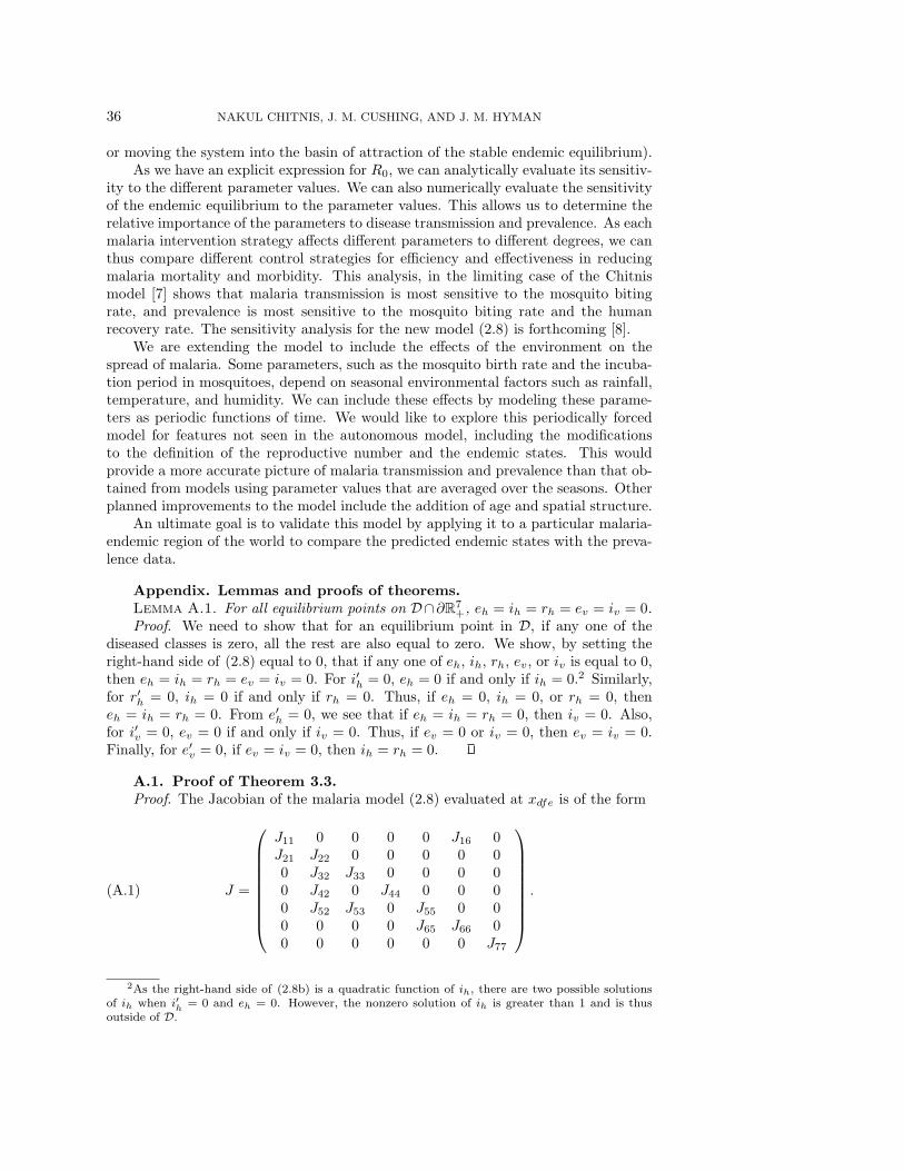
A.1. Proof of Theorem 3.3.Proof. The Jacobian of the malaria model (2.8) evaluated at xdfe is of the form

J =

⎛⎜⎜⎜⎜⎜⎜⎜⎜⎝

J11 0 0 0 0 J16 0J21 J22 0 0 0 0 00 J32 J33 0 0 0 00 J42 0 J44 0 0 00 J52 J53 0 J55 0 00 0 0 0 J65 J66 00 0 0 0 0 0 J77

⎞⎟⎟⎟⎟⎟⎟⎟⎟⎠

.(A.1)

2As the right-hand side of (2.8b) is a quadratic function of ih, there are two possible solutionsof ih when i′h = 0 and eh = 0. However, the nonzero solution of ih is greater than 1 and is thusoutside of D.


As the fourth and seventh columns (corresponding to the total human and mosquitopopulations) contain only the diagonal terms, these diagonal terms form two eigen-values of the Jacobian:

η6 = ψh − μ1h − 2μ2hN∗h = −

√(ψh − μ1h)2 + 4μ2hΛh,(A.2a)

η7 = ψv − μ1v − 2μ2vN∗v = −(ψv − μ1v).(A.2b)

As we have assumed that ψv > μ1v, both η6 and η7 are always negative. The otherfive eigenvalues are the roots of the characteristic equation of the matrix formed byexcluding the fourth and seventh rows and columns of the Jacobian (A.1):

A5η5 + A4η

4 + A3η3 + A2η

2 + A1η + A0 = 0(A.3)

with

A5 = 1,

A4 = B1 + B2 + B3 + B4 + B5,

A3 = B1B2 + B1B3 + B1B4 + B1B5 + B2B3 + B2B4 + B2B5 + B3B4

+ B3B5 + B4B5,

A2 = B1B2B3 + B1B2B4 + B1B2B5 + B1B3B4 + B1B3B5 + B1B4B5 + B2B3B4

+ B2B3B5 + B2B4B5 + B3B4B5,

A1 = B1B2B3B4 + B1B2B3B5 + B1B2B4B5 + B1B3B4B5 + B2B3B4B5

−B6B7B8B9,

A0 = B1B2B3B4B5 − (B3B6B7B8B9 + B6B7B9B10B11),

and B1 = νh + ψh + Λh/N∗h , B2 = γh + δh + ψh + Λh/N

∗h , B3 = ρh + ψh + Λh/N

∗h ,

B4 = νv + ψv, B5 = ψv, B6 = b∗hβhv, B7 = νh, B8 = b∗vβvh, B9 = νv, B10 = γh, and

B11 = b∗vβvh.To evaluate the signs of the roots of (A.3), we first use the Routh–Hurwitz cri-

terion to prove that when R0 < 1, all roots of (A.3) have negative real part. Then,using Descartes’s rule of sign, we prove that when R0 > 1, there is one positive realroot.

The Routh–Hurwitz criterion [18, section 1.6-6(b)] for a real algebraic equation

anxn + an−1x

n−1 + · · · + a1x + a0 = 0(A.4)

states that, given an > 0, all roots have negative real part if and only if T0 = an,T1 = an−1,

T2 =

∣∣∣∣ an−1 anan−3 an−2

∣∣∣∣ , T3 =

∣∣∣∣∣∣an−1 an 0an−3 an−2 an−1

an−5 an−4 an−3

∣∣∣∣∣∣ , . . . , Tn =

∣∣∣∣∣∣∣an−1 · · · 0

.... . .

...0 · · · a0

∣∣∣∣∣∣∣are all positive, with ai = 0 for i < 0. This is true if and only if all ai and either alleven-numbered Tk or all odd-numbered Tk are positive (the Lienard–Chipart test).Korn and Korn [18] in section 1.6-6(c) state Descartes’s rule of sign as the numberof positive real roots of a real algebraic equation (A.4) is equal to the number, Na,of sign changes in the sequence, an, an−1, . . . , a0, of coefficients, where the vanishingterms are disregarded, or it is less than Na by a positive even integer.


We show that when R0 < 1, all the coefficients, Ai, of the characteristic equation(A.3), and T0, T2, and T4, are positive, so by the Routh–Hurwitz criterion, all theeigenvalues of the Jacobian (A.1) have negative real part. We then show that whenR0 > 1, there is one and only one sign change in the sequence A5, A4, . . . , A0, soby Descartes’s rule of sign there is one eigenvalue with positive real part, and thedisease-free equilibrium point is unstable.

The expression for R20 in (3.4) can be written, in terms of Bi, as

R20 =

B3B6B7B8B9 + B6B7B9B10B11

B1B2B3B4B5.(A.5)

For R0 < 1, by (A.5),

B3B6B7B8B9 + B6B7B9B10B11 < B1B2B3B4B5,(A.6)

B6B7B8B9 < B1B2B4B5.(A.7)

As all the Bi are positive, A5, A4, A3, and A2 are always positive. From (A.7) wesee that A1 > 0, and from (A.6) we see that A0 > 0. Thus, for R0 < 1, all Ai arepositive. We now show that the even-numbered Tk are positive for R0 < 1. For thefifth-degree polynomial (A.3), T0 = A5, which is always positive. T2 = A3A4 −A2A5,which we can show to be a positive sum of products of Bi’s, so T2 > 0. Lastly,

T4 = A1[A2A3A4 − (A1A24 + A2

2A5)] −A0[A3(A3A4 −A2A5) − (2A1A4A5 −A0A25)].

For ease of notation, we introduce

C1 = A2A3A4 − (A1A24 + A2

2A5),

C2 = A3(A3A4 −A2A5) − (2A1A4A5 −A0A25),

where we can show that C1 > 0 and C2 > 0, so that T4 = A1C1 −A0C2. We define

C(1)2 = C2 + B6B7B9B10B11.

As C(1)2 > C2 and A0 > 0, for T

(1)4 = A1C1 −A0C

(1)2 , T4 > T

(1)4 . Similarly, we define

A(1)0 = A0 + (B3B6B7B8B9 + B6B7B9B10B11).

As A(1)0 > A0 and C

(1)2 > 0, for T

(2)4 = A1C1 − A

(1)0 C

(1)2 , T

(1)4 > T

(2)4 . Finally, we

define

A(1)1 = A1 − (B1B2B4B5 −B6B7B8B9).

As A(1)1 < A1 (for R0 < 1) and C1 > 0, for T

(3)4 = A

(1)1 C1−A

(1)0 C

(1)2 , T

(2)4 > T

(3)4 . We

can show that T(3)4 is a sum of positive terms, so T

(3)4 > 0. As T4 > T

(1)4 > T

(2)4 > T

(3)4 ,

T4 > 0. Thus, for R0 < 1, all roots of (A.3) have negative real parts.When R0 > 1

B3B6B7B8B9 + B6B7B9B10B11 > B1B2B3B4B5,

and so A0 < 0. As A5, A4, A3, and A2 are positive, the sequence, A5, A4, A3, A2, A1, A0

has exactly one sign change. Thus, by Descartes’s rule of sign, (A.3) has one positivereal root when R0 > 1.


Thus, the disease-free equilibrium point, xdfe, is locally asymptotically stable ifR0 < 1 and unstable if R0 > 1. If R0 < 1, on average each infected individual infectsfewer than one other individual, and the disease dies out. If R0 > 1, on average eachinfected individual, infects more than one other individual, so we would expect thedisease to spread. The Jacobian of (2.8) at xdfe has one eigenvalue equal to 0 atR0 = 1.

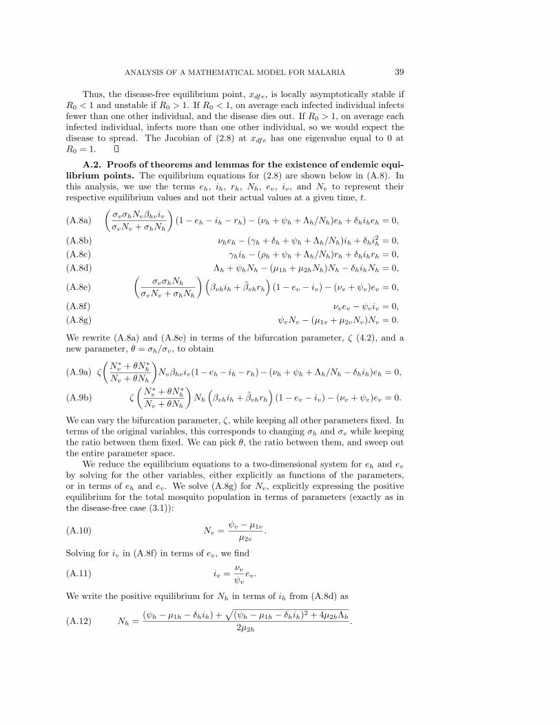
A.2. Proofs of theorems and lemmas for the existence of endemic equi-librium points. The equilibrium equations for (2.8) are shown below in (A.8). Inthis analysis, we use the terms eh, ih, rh, Nh, ev, iv, and Nv to represent theirrespective equilibrium values and not their actual values at a given time, t.(

σvσhNvβhvivσvNv + σhNh

)(1 − eh − ih − rh) − (νh + ψh + Λh/Nh)eh + δhiheh = 0,(A.8a)

νheh − (γh + δh + ψh + Λh/Nh)ih + δhi2h = 0,(A.8b)

γhih − (ρh + ψh + Λh/Nh)rh + δhihrh = 0,(A.8c)

Λh + ψhNh − (μ1h + μ2hNh)Nh − δhihNh = 0,(A.8d) (σvσhNh

σvNv + σhNh

)(βvhih + βvhrh

)(1 − ev − iv) − (νv + ψv)ev = 0,(A.8e)

νvev − ψviv = 0,(A.8f)

ψvNv − (μ1v + μ2vNv)Nv = 0.(A.8g)

We rewrite (A.8a) and (A.8e) in terms of the bifurcation parameter, ζ (4.2), and anew parameter, θ = σh/σv, to obtain

ζ

(N∗

v + θN∗h

Nv + θNh

)Nvβhviv(1− eh − ih − rh)− (νh + ψh + Λh/Nh − δhih)eh = 0,(A.9a)

ζ

(N∗

v + θN∗h

Nv + θNh

)Nh

(βvhih + βvhrh

)(1 − ev − iv) − (νv + ψv)ev = 0.(A.9b)

We can vary the bifurcation parameter, ζ, while keeping all other parameters fixed. Interms of the original variables, this corresponds to changing σh and σv while keepingthe ratio between them fixed. We can pick θ, the ratio between them, and sweep outthe entire parameter space.

We reduce the equilibrium equations to a two-dimensional system for eh and evby solving for the other variables, either explicitly as functions of the parameters,or in terms of eh and ev. We solve (A.8g) for Nv, explicitly expressing the positiveequilibrium for the total mosquito population in terms of parameters (exactly as inthe disease-free case (3.1)):

Nv =ψv − μ1v

μ2v.(A.10)

Solving for iv in (A.8f) in terms of ev, we find

iv =νvψv

ev.(A.11)

We write the positive equilibrium for Nh in terms of ih from (A.8d) as

Nh =(ψh − μ1h − δhih) +

√(ψh − μ1h − δhih)2 + 4μ2hΛh

2μ2h.(A.12)


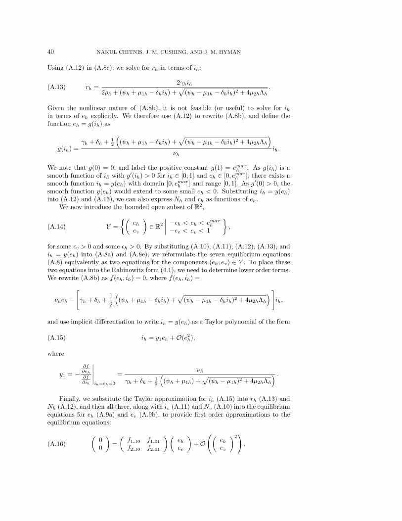
Using (A.12) in (A.8c), we solve for rh in terms of ih:

rh =2γhih

2ρh + (ψh + μ1h − δhih) +√

(ψh − μ1h − δhih)2 + 4μ2hΛh

.(A.13)

Given the nonlinear nature of (A.8b), it is not feasible (or useful) to solve for ihin terms of eh explicitly. We therefore use (A.12) to rewrite (A.8b), and define thefunction eh = g(ih) as

g(ih) =γh + δh + 1

2

((ψh + μ1h − δhih) +


)νh

ih.

We note that g(0) = 0, and label the positive constant g(1) = emaxh . As g(ih) is a

smooth function of ih with g′(ih) > 0 for ih ∈ [0, 1] and eh ∈ [0, emaxh ], there exists a

smooth function ih = y(eh) with domain [0, emaxh ] and range [0, 1]. As g′(0) > 0, the

smooth function y(eh) would extend to some small eh < 0. Substituting ih = y(eh)into (A.12) and (A.13), we can also express Nh and rh as functions of eh.

We now introduce the bounded open subset of R2,

Y =

{(ehev

)∈ R

2

∣∣∣∣ −εh < eh < emaxh

−εv < ev < 1

},(A.14)

for some εv > 0 and some εh > 0. By substituting (A.10), (A.11), (A.12), (A.13), andih = y(eh) into (A.8a) and (A.8e), we reformulate the seven equilibrium equations(A.8) equivalently as two equations for the components (eh, ev) ∈ Y . To place thesetwo equations into the Rabinowitz form (4.1), we need to determine lower order terms.We rewrite (A.8b) as f(eh, ih) = 0, where f(eh, ih) =

νheh −[γh + δh +

1

2

((ψh + μ1h − δhih) +


)]ih,

and use implicit differentiation to write ih = y(eh) as a Taylor polynomial of the form

ih = y1eh + O(e2h),(A.15)

where

y1 = −∂f∂eh∂f∂ih

∣∣∣∣∣ih=eh=0

=νh

γh + δh + 12

((ψh + μ1h) +

√(ψh − μ1h)2 + 4μ2hΛh

) .

Finally, we substitute the Taylor approximation for ih (A.15) into rh (A.13) andNh (A.12), and then all three, along with iv (A.11) and Nv (A.10) into the equilibriumequations for eh (A.9a) and ev (A.9b), to provide first order approximations to theequilibrium equations:

(00

)=

(f1 10 f1 01

f2 10 f2 01

)(ehev

)+ O

((ehev

)2),(A.16)


where

f1 10 = −[νh +

1

2

((ψh + μ1h) +

√(ψh − μ1h)2 + 4μ2hΛh

)],(A.17a)

f1 01 = ζ · νvβhv(ψv − μ1v)

ψvμ2v,(A.17b)

f2 10 = ζ ·νh

((ψh − μ1h) +

√(ψh − μ1h)2 + 4Λhμ2h

)2μ2h

(γh + δh + 1

2

((ψh + μ1h) +

√(ψh − μ1h)2 + 4μ2hΛh

))(A.17c)

×

⎡⎣βvh +

γhβvh

ρh + 12

((ψh + μ1h) +

√(ψh − μ1h)2 + 4μ2hΛh

)⎤⎦ ,

f2 01 = − (ψv + νv) .(A.17d)

To apply Corollary 1.12 of Rabinowitz [24], we algebraically manipulate (A.16)to produce

u = ζLu + h(ζ, u),(A.18)

where

u =

(ehev

)and L =

(0 AB 0

)with

A =νvβhv(ψv − μ1v)

ψvμ2v

(νh + 1

2

((ψh + μ1h) +

√(ψh − μ1h)2 + 4μ2hΛh

)) ,(A.19a)

B =

⎛⎝βvh +

γhβvh

ρh + 12

((ψh + μ1h) +

√(ψh − μ1h)2 + 4μ2hΛh

)⎞⎠(A.19b)

×νh

((ψh − μ1h) +

√(ψh − μ1h)2 + 4μ2hΛh

)2μ2h(ψv + νv)

(γh + δh + 1

2

((ψh +μ1h)+

√(ψh −μ1h)2 + 4μ2hΛh

)) ,

and h(ζ, u) is O(u2). The matrix, L, has two distinct eigenvalues: ±√AB. Charac-

teristic values of a matrix are the reciprocals of its eigenvalues. We denote the twocharacteristic values of L by ξ1 = 1/

√AB and ξ2 = −1/

√AB. As both A and B are

always positive (because we have assumed that ψv > μ1v), ξ1 is real and correspondsto the dominant eigenvalue of L. The right and left eigenvectors corresponding to ξ1are, respectively,

v =

(√A√B

)and w =

(√B

√A).(A.20)

For MZ > ξ1, as 0 ∈ Y , (ξ1, 0) ∈ Ω. By Corollary 1.12 of Rabinowitz [24], weknow that there is a continuum of solution-pairs (ζ, u) ∈ Ω, whose closure containsthe point (ξ1, 0), that either meets the boundary of Ω, ∂Ω, or the point (ξ2, 0). We


denote the continuum of solution-pairs emanating from (ξ1, 0) by C1, where C1 ⊂ Ω,and from (ξ2, 0) by C2, where C2 ⊂ Ω. We introduce the sets

Z1 = {ζ ∈ Z| ∃u such that (ζ, u) ∈ C1} ,(A.21a)

U1 = {u ∈ Y | ∃ζ such that (ζ, u) ∈ C1} ,(A.21b)

Z2 = {ζ ∈ Z| ∃u such that (ζ, u) ∈ C2} ,(A.21c)

U2 = {u ∈ Y | ∃ζ such that (ζ, u) ∈ C2} .(A.21d)

We denote the part of Y in the positive quadrant of R2 by Y + = {(eh, ev) ∈ Y | eh >

0 and ev > 0}, and the internal boundary of Y + by

∂Y + =

⎧⎨⎩(

ehev

)∈ Y

∣∣∣∣∣∣⎛⎝ eh > 0

andev = 0

⎞⎠ or

⎛⎝ eh = 0

andev > 0

⎞⎠ or

⎛⎝ eh = 0

andev = 0

⎞⎠⎫⎬⎭ .

We can determine the initial direction of the continua of solution-pairs, C1 andC2, using the Lyapunov–Schmidt expansion, as described by Cushing [9]. Althoughwe show the proofs only for the expansion of C1 around the bifurcation point at ζ = ξ1in Lemmas A.2 and A.3, the results for C2 around ζ = ξ2 are similar. We begin byexpanding the terms of the nonlinear eigenvalue equation (A.18) about the bifurcationpoint, (ξ1, 0). The expanded variables are

u = 0 + εu(1) + ε2u(2) + · · · ,(A.22a)

ζ = ξ1 + εζ1 + ε2ζ2 + · · · ,(A.22b)

h(ζ, u) = h(ξ1 + εζ1 + ε2ζ2 + · · · , εu(1) + ε2u(2) + · · · )(A.22c)

= ε2h2(ξ1, u(1)) + · · · .

We substitute the expansions (A.22) into the eigenvalue equation (A.18) and evaluateat different orders of ε. Evaluating the substitution of the expansions (A.22) into theeigenvalue equation (A.18) at O(ε0) produces 0 = 0, which gives us no information.

Lemma A.2. The initial direction of the branch of equilibrium points, u(1), nearthe bifurcation point, (ξ1, 0), is equal to the right eigenvector of L corresponding tothe characteristic value, ξ1.

Proof. Evaluating the substitution of the expansions (A.22) into the eigenvalueequation (A.18) at O(ε1), we obtain u(1) = ξ1Lu

(1). This implies that u(1) is theright eigenvector of L corresponding to the eigenvalue 1/ξ1, v (A.20). Thus, close tothe bifurcation point, the equilibrium point can be approximated by eh = ε

√A and

ev = ε√B.

Lemma A.3. The bifurcation at ζ = ξ1 of the nonlinear eigenvalue equation(A.18) is supercritical if ζ1 > 0 and subcritical if ζ1 < 0, where

ζ1 = −w · h2

w · Lv ,(A.23)

where v and w are the right and left eigenvectors of L corresponding to the character-istic value ξ1, respectively.

Proof. Evaluating the substitution of the expansions (A.22) into the eigenvalueequation (A.18) at O(ε2), we obtain u(2) = ξ1Lu

(2) + ζ1Lu(1) + h2, which we can


rewrite as

(I − ξ1L)u(2) = ζ1Lv + h2,(A.24)

where I is the 2 × 2 identity matrix. As ξ1 is a characteristic value of L, (I − ξ1L)is a singular matrix. Thus, for (A.24) to have a solution, ζ1Lv + h2 must be in therange of (I − ξ1L); i.e., it must be orthogonal to the null space of the adjoint of(I− ξ1L). The null space of the adjoint of (I− ξ1L) is spanned by the left eigenvectorof L (corresponding to the eigenvalue 1/ξ1), w (A.20). The Fredholm condition forthe solvability of (A.24) is w · (ζ1Lv + h2) = 0. Solving for ζ1 provides (A.23). Ifζ1 is positive, then for small positive ε, u > 0 and ζ > ξ1, and the bifurcation issupercritical. Similarly, if ζ1 is negative, then for small positive ε, u > 0 and ζ < ξ1,and the bifurcation is subcritical.

Lemma A.4. For all u ∈ U1, eh > 0 and ev > 0.Proof. By Lemma A.1, there are no equilibrium points on ∂Y + other than eh =

ev = 0, so U1 ∩ ∂Y + = 0. We know from Lemma A.2 that close to the bifurcationpoint (ξ1, 0), the direction of U1 is equal to v, the right eigenvector corresponding tothe characteristic value, ξ1. As v contains only positive terms, U1 is entirely containedin Y +. Thus, for all u ∈ U1, eh > 0 and ev > 0.

Lemma A.5. The point u = 0 ∈ Y corresponds to xdfe ∈ R7 (on the boundary

of the positive orthant of R7). For every solution-pair (ζ, u) ∈ C1, there corresponds

one equilibrium-pair (ζ, x∗) ∈ Z × R7, where x∗ is in the positive orthant of R

7.Proof. We first show that u = 0 corresponds to xdfe. As eh = ev = 0, by

Theorem 3.1 we know that the only possible equilibrium point is xdfe. We nowshow that for every ζ ∈ Z1 there exists an x∗ in the positive orthant of R

7 for thecorresponding u ∈ U1. By Lemma A.4, we know that eh > 0 and ev > 0. We nowneed to show that for every positive eh and ev there exist corresponding positive ih,rh, iv, Nh, and Nv. By looking at the equilibrium equation for iv (A.11), we see thatfor every positive ev there exists a positive iv. The equilibrium equation for Nv hasa positive and bounded solution, depending only on parameter values (A.10). Fromih = y(eh), we see that for every positive eh there exists a positive ih. The equilibriumequations for rh (A.13) and Nh (A.12) show that for every positive ih there exists apositive rh and Nh.

Lemma A.6. The set U1 does not meet the boundary of Y .Proof. As Lemma A.4 shows us that for all u ∈ U1, eh > 0 and ev > 0, we need

to show that eh < emaxh and ev < 1. By Lemma A.5, we know that all state variables

are positive. Therefore, for (A.8e) to have a solution, ev + iv < 1 so ev < 1. Fromthe properties of eh = g(ih), we know that as ih increases, eh increases monotonically,reaching emax

h at ih = 1. However, we have already shown that when eh + ih +rh = 1,e′h + i′h + r′h < 0, and thus there can be no equilibrium point at eh + ih + rh = 1.Therefore, ih is always less than 1, and eh is always less than emax

h .Proof of Theorem 4.1. As shown in Lemma A.4, U1 ∩ ∂Y + = 0 and U1 is entirely

contained in Y +. We can similarly show that U2 is entirely outside of Y + because theright eigenvector corresponding to ξ2 is ( −

√A

√B )T. Therefore, C1 and C2 do

not intersect, and by Corollary 1.12 of Rabinowitz [24], C1 meets ∂Ω. By Lemma A.6,the set U1 does not meet the boundary of Y , so C1 meets ∂Ω only at ζ = MZ .

By Lemma A.5, for every u ∈ U1, there corresponds an x∗ in the positive orthantof R

7, and u = 0 corresponds to xdfe (on the boundary of the positive orthant of R7).

Thus, there exists a continuum of equilibrium-pairs (ζ, x∗) ∈ Z × R7 that connects

the point (ξ1, xdfe) to the hyperplane ζ = MZ in R × R7.


Proof of Theorem 4.3. When δh = 0, we can explicitly evaluate h(ζ, u) in thenonlinear eigenvalue equation (A.18) from the equilibrium equations (A.8) as

h = ζ

(C(δh=0)ehevD(δh=0)ehev

)(A.25)

since the coefficients of all the other higher order terms are zero. Although we donot show the explicit representations for C(δh=0) and D(δh=0), they are both negative.From (A.25) and (A.22) we can evaluate the second order expansion

h2 = ξ1

(C(δh=0)

√A√B

D(δh=0)

√A√B

)=

(C(δh=0)

D(δh=0)

).(A.26)

As h2 contains only negative terms and w, v, and L contain only nonnegative terms,(A.23) implies that ζ1 is positive. Thus, by Lemma A.3, with no disease-induceddeath, for any positive values of the other parameters there is a supercritical bifurca-tion at R0 = 1.

Acknowledgements. The authors thank Karl Hadeler for his discussions andideas on improving the model, including the mosquitoes’ human-biting rates; AlainGoriely, Joceline Lega, Jia Li, Seymour Parter, and Joel Miller for their careful readingof the manuscript and valuable comments; and two anonymous referees for manyhelpful suggestions.

REFERENCES

[1] R. M. Anderson and R. M. May, Infectious Diseases of Humans: Dynamics and Control,Oxford University Press, Oxford, UK, 1991.

[2] J. L. Aron, Mathematical modeling of immunity to malaria, Math. Biosci., 90 (1988), pp. 385–396.

[3] J. L. Aron and R. M. May, The population dynamics of malaria, in The Population Dynamicsof Infectious Disease: Theory and Applications, R. M. Anderson, ed., Chapman and Hall,London, 1982, pp. 139–179.

[4] N. Bacaer and C. Sokhna, A reaction-diffusion system modeling the spread of resistance toan antimalarial drug, Math. Biosci. Engrg., 2 (2005), pp. 227–238.

[5] N.J.T. Bailey, The Mathematical Theory of Infectious Diseases and Its Application, Griffin,London, 1975.

[6] C. Castillo-Chavez and B. Song, Dynamical models of tuberculosis and their applications,Math. Biosci. Engrg., 1 (2004), pp. 361–404.

[7] N. Chitnis, Using Mathematical Models in Controlling the Spread of Malaria, Ph.D. thesis,Program in Applied Mathematics, University of Arizona, Tucson, AZ, 2005.

[8] N. Chitnis, J. M. Hyman, and J. M. Cushing, Determining Important Parameters in theSpread of Malaria Through the Sensitivity Analysis of a Mathematical Model, in prepara-tion.

[9] J. M. Cushing, An Introduction to Structured Population Dynamics, CBMS-NSF Reg. Conf.Ser. Appl. Math. 71, SIAM, Philadelphia, 1998.

[10] O. Diekmann, J.A.P. Heesterbeek, and J.A.J. Metz, On the definition and the computa-tion of the basic reproduction ratio R0 in models for infectious diseases in heterogeneouspopulations, J. Math. Biol., 28 (1990), pp. 365–382.

[11] K. Dietz, L. Molineaux, and A. Thomas, A malaria model tested in the African savannah,Bull. World Health Organ., 50 (1974), pp. 347–357.

[12] E. J. Doedel, R. C. Paffenroth, A. R. Champneys, T. F. fairgrieve, Y. A. Kuznetsov, B.

Sandstede, and X. Wang, AUTO 2000: Continuation and Bifurcation Software for Or-dinary Differential Equations (with HomCont), v.0.9.7, 2002; online at http://sourceforge.net/projects/auto2000/.

[13] H. Gomez-Acevedo and M. Y. Li, Backward bifurcation in a model for HTLV-I infection ofCD4+ T cells, Bull. Math. Biol., 67 (2005), pp. 101–114.


[14] J. M. Hyman and J. Li, An intuitive formulation for the reproductive number for the spreadof diseases in heterogeneous populations, Math. Biosci., 167 (2000), pp. 65–86.

[15] J. C. Koella, On the use of mathematical models of malaria transmission, Acta Tropica, 49(1991), pp. 1–25.

[16] J. C. Koella and R. Antia, Epidemiological models for the spread of anti-malarial resistance,Malaria J., 2 (2003).

[17] J. C. Koella and C. Boete, A model for the coevolution of immunity and immune evasionin vector-borne disease with implications for the epidemiology of malaria, The AmericanNaturalist, 161 (2003), pp. 698–707.

[18] G. A. Korn and T. M. Korn, Mathematical Handbook for Scientists and Engineers: Defini-tions, Theorems, and Formulas for Reference and Review, Dover Publications, Mineola,NY, 2000.

[19] J. Li, R. M. Welch, U. S. Nair, T. L. Sever, D. E. Irwin, C. Cordon-Rosales, and

N. Padilla, Dynamic malaria models with environmental changes, in Proceedings of theThirty-Fourth Southeastern Symposium on System Theory, Huntsville, AL, 2002, pp. 396–400.

[20] G. Macdonald, The Epidemiology and Control of Malaria, Oxford University Press, London,1957.

[21] J. Nedelman, Introductory review: Some new thoughts about some old malaria models, Math.Biosci., 73 (1985), pp. 159–182.

[22] G. A. Ngwa, Modelling the dynamics of endemic malaria in growing populations, DiscreteContin. Dyn. Syst. Ser. B, 4 (2004), pp. 1173–1202.

[23] G. A. Ngwa and W. S. Shu, A mathematical model for endemic malaria with variable humanand mosquito populations, Math. Comput. Modelling, 32 (2000), pp. 747–763.

[24] P. H. Rabinowitz, Some global results for nonlinear eigenvalue problems, J. Funct. Anal., 7(1971), pp. 487–513.

[25] R. Ross, The Prevention of Malaria, John Murray, London, 1911.[26] P. van den Driessche and J. Watmough, A simple SIS epidemic model with a backward

bifurcation, J. Math. Biol., 40 (2000), pp. 525–540.[27] H. M. Yang, Malaria transmission model for different levels of acquired immunity and

temperature-dependent parameters (vector), Revista de Saude Publica, 34 (2000), pp. 223–231.

[28] H. M. Yang and M. U. Ferreira, Assessing the effects of global warming and local social andeconomic conditions on the malaria transmission, Revista de Saude Publica, 34 (2000),pp. 214–222.

Documents

BIFURCATION ANALYSIS OF A MATHEMATICAL MODEL FOR