Bifurcation Analysis of a CoupledNose Landing Gear-Fuselage System

Nandor Terkovics, Simon Neild, Mark LowenbergFaculty of Engineering, University of Bristol, Bristol, BS8 1TR, UK

Bernd KrauskopfDepartment of Mathematics, The University of Auckland,

Private Bag 92019, Auckland 1142, New Zealand

February 2013

Abstract

Under certain conditions during take-off and landing, pilots may sometimes experience vibrations in thecockpit. Since the cockpit is located right above the nose landing gear – which is known to potentiallybe prone to self-excited vibrations at certain velocities – an explanation for those vibrations might beoscillations of the landing gear feeding into the fuselage. However, the fuselage dynamics itself may alsoinfluence the dynamics of the landing gear, meaning that the coupling must be considered as bi-directional.A mathematical model is developed to study a coupled nose landing gear-fuselage system, which allows toassess the overall influence of the coupling on the system dynamics. Bifurcation analysis reveals that thisinteraction may be significant in both directions, and that the system behaviour depends strongly on themodal characteristics of the fuselage.

1 Introduction

At the design and testing stage of an aircraft, vibrations during take-off and landing, especially in the cockpit,must be considered to ensure that they remain small. A potential source of such oscillations is via the dynamicinteraction between the fuselage rigid-body and/or flexible modes and the nose landing gear system when theaircraft is in motion on the ground.

It is well known that wheeled vehicles can experience self-excited wheel vibrations under certain conditions.The phenomenon, referred to as shimmy, has interested researchers since the late 1940s when von Schlippe andDietrich [1] published the first results on the dynamics of elastic tyres and gave the first explanation for shimmyby the so called “stretched string tyre model”. In that model the tyre-ground interface is considered as a contactline that becomes deformed due to the lateral displacement of the tyre; the contact line is modeled as a straightline between the leading and trailing points. Pacejka [2, 3, 4] extended the stretched string tyre model byapproximating the contact line with various stationary shape functions, and incorporated it into various vehiclemodels. He showed both theoretically and experimentally that periodic and quasi-periodic shimmy oscillationsmay occur in flexible wheeled structures. As another approach, the“exact stretched string tyre model” of Segel[5] models the contact line without any restrictions to the shape and so considers the actual and dynamicallyvarying shape of the contact region. Stepan [6] used the exact stretched string tyre model and studied a singledegree-of-freedom pulled trailer by means of nonlinear techniques. In that study the mathematical model is givenas a coupled partial differential – integro-differential equation system, where the partial differential part has atravelling wave-like solution, which introduces time delay into the system. This model was further extendedand experimentally tested by Takacs et al. [7, 8].

A nose landing gear (referred to as NLG), fitted with an elastic tyre and having structural flexibilities, canalso experience shimmy oscillations, and these have been of interest since aircrafts exist. Smiley [9] used linear

1

techniques to study three different landing gear configurations and to correlate different tyre models. Morerecently Somieski [10] introduced nonlinearities into the existing landing gear models and found supercriticalHopf bifurcations and stable limit cycles and, hence, gave an explanation for the onset of shimmy. Recentresults on the topic were published by Thota et al.[11, 12]. In those studies, not only is a non-zero rake angleconsidered, but also a lateral degree-of-freedom is introduced to the landing gear model; the torsional and lateraldegrees-of-freedom are coupled via the lateral deformation of the tyre. The body of the aircraft is considered as ablock of mass that exerts a fixed vertical force Fz on the gear while the aircraft is moving at a forward velocity V[11, 12]. This approach allows one to determine the occurrence of (different types of) shimmy oscillations in the(V, Fz)-plane. The analysis showed that, beyond stable torsional shimmy oscillations, stable lateral vibrationscan also be triggered. Furthermore, a large region of bistability, where both types of shimmy oscillations arepossible, was found, as well as quasi-periodic shimmy oscillations [11, 12]. The term shimmy, which historicallyonly referred to the torsional vibrations of wheels and wheeled structures, is, therefore, used here to describemore general mechanical vibrations in aircraft landing gears or other tyred systems.

During ground manoeuvres the aircraft is supported by the landing gears. Therefore, oscillations of thelanding gears are potential sources of excitation for the aircraft body. In particular, the oscillation of theNLG, which is attached to the fuselage and located right below the cockpit may feed directly into the fuselageand excite vibrations in the cockpit. On the other hand, an oscillating aircraft body can also influence thebehaviour of the NLG. In order to clarify this mutual interaction, a coupled NLG-fuselage system is developedand analysed here.

A second motivation for the coupling is the wish to evaluate the feasibilty of the application of real-timedynamic substructuring (RTDS) [13, 14] to the NLG-fuselage system. Real-time dynamic substructuring isan effective way of testing complicated systems, where complete numerical modelling or experimental testing isdifficult. In an RTDS-test, a part of the physical system is experimentally tested and the remainder is modellednumerically. Advanced real-time control techniques are used to effectively ‘glue together’ the test specimen andthe numerical model of the remainder of the system, via a transfer system (ie. actuators). Through displace-ment control of the actuators and force feedback to the numerical model the physical-numerical interface canbe matched, so that the dynamics of the overall system is replicated [13, 14]. A natural choice for the testcomponent in the present context is the entire nose landing gear, which is coupled to a numerical model of thefuselage. However, for an RTDS-test to be reasonable, sufficient force or displacement feedback is essential. Inour case this means significant interaction between the fuselage and the landing gear. Therefore, in order tostudy the feasibilty of an RTDS-test on a landing gear-fuselage system, not only do we need to examine theinteraction itself, but we also have to study when it is significant to provide sufficient feedback.

The coupled model considers the same landing gear configuration as that of [12]. However, beside beingcoupled via the tyre only, the landing gear modes here considered are coupled directly as well via the geometryof the strucure. Part of this extended NLG model is the dynamic model of the fuselage, which is – for simplicity– represented by a second-order linear mass-spring-damper unit (referred to as MSD) attached to the top ofthe landing gear strut. The MSD is characterized by its natural frequency, relative damping and an effective(modal) mass. Further, the effective fuselage weight acting on the NLG, when the system is in equlibrium, andthe weight of the NLG are represented by static, vertical forces. The exact stretched string tyre model completesthe system; however, only the leading point of the contact region is considered to calculate the tyre force and,hence, the time delay is not taken into account. The potential mutual interaction between the landing gear andthe fuselage is then studied for this coupled model, with special interest in the effect of different modal masses;to this end numerical bifurcation analysis is used, specifically the continuation software AUTO [15].

The analysis reveals that, when the forward velocity is varied, the straight rolling solution loses its stabiltyvia Hopf-bifurcations; the system can experience stable periodic oscillations dominated by either lateral ortorsional oscillations of the NLG. It is also shown that, in general, the lower the modal mass, the higher theamplitude of the emerging fuselage vibrations, hence, the more energy is fed into the fuselage from the NLG.On the other hand, a change in the modal mass not only changes the fuselage amplitudes, but also influencesthe regions of stability and, at certain velocities, the type of oscillation; i.e. a dominantly torsional oscillationcan change to lateral- or even quasi-periodic oscillations. However, this effect is strongly influenced by the loadas well. To show these results in detail, one- and two-parameter bifurcation diagrams are presented.

2

.

.

(a) (b)

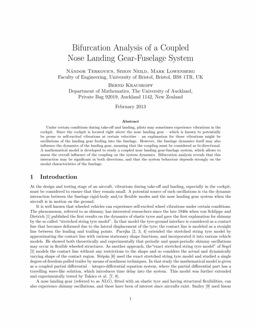
Figure 1: Illustrations of the considered fuselage dynamics. Panel (a) and (b) show modes with exagerrated lateraldeformation of the fuselage, and rigid body oscillation about the vertical body axis, respectively.

2 The Model

2.1 A low-order fuselage model

Due to the nature of the NLG-fuselage system, a coupled, constrained model is required, that incorporatesseparate models for both the NLG and the fuselage, and is completed by the tyre model. Both the NLG modelof [12] – the configuration of which is used here –, and the tyre model are highly nonlinear. Owing to low fuselageamplitudes, a low order, linear model is used to represent the fuselage dynamics. Out of the many considerablemodes of a fuselage, only those with lateral displacement component at the attachment point are considered inthis study. That displacement can be the result of either a modal oscillation leading to deformation at the frontof the fuselage or, alternatively, a rigid body mode corresponding to the torsional oscillation of the fuselageabout its vertical body axis; see Figure 1.

In the first case we assume an elastic fuselage and allow modal dynamics, whereas in the second case weassume that, while moving forward on the runway, the aircraft oscillates torsionally about its centre of mass asa rigid body. In either case, the amplitudes of oscillations are assumed to be small compared to the wheelbaseof the aircraft. Therefore, the motion of the attachment point is taken as linear translation and, hence, itsdynamics is modelled by a linear mass-spring-damper system (MSD). It is characterized by its natural frequencyfn, relative damping q and modal mass µ corresponding to the considered mode, and also by the lateral fuselagedisplacement y. Moreover, the mass is allowed to move up and down introducing a vertical displacement z;however, this motion is constrained to follow the vertical component of translation of the top of the landinggear system, which leaves y as the only fuselage degree-of-freedom; see Section 2.3 for details of the verticalconstraint. Further, the proportion of the weight M of the aircraft, that is supported by the NLG, when theaircraft is on the ground, and the weight m of the NLG are considered by the corresponding gravitational forces.

2.2 The landing gear model

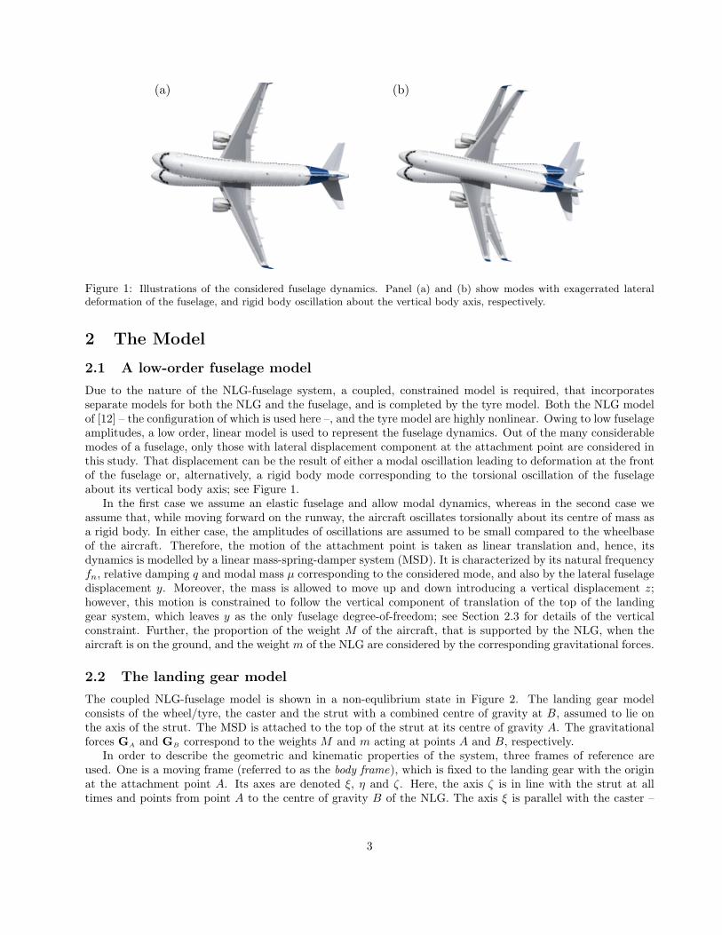
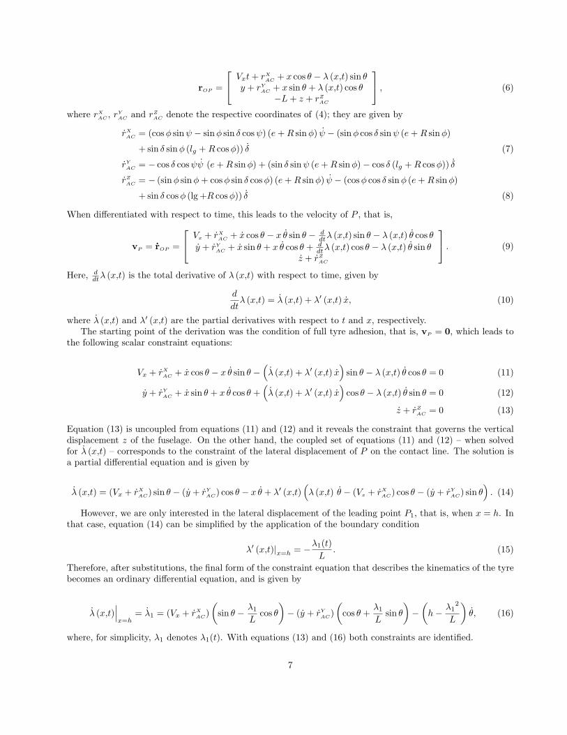
The coupled NLG-fuselage model is shown in a non-equlibrium state in Figure 2. The landing gear modelconsists of the wheel/tyre, the caster and the strut with a combined centre of gravity at B, assumed to lie onthe axis of the strut. The MSD is attached to the top of the strut at its centre of gravity A. The gravitationalforces GA and GB correspond to the weights M and m acting at points A and B, respectively.

In order to describe the geometric and kinematic properties of the system, three frames of reference areused. One is a moving frame (referred to as the body frame), which is fixed to the landing gear with the originat the attachment point A. Its axes are denoted ξ, η and ζ. Here, the axis ζ is in line with the strut at alltimes and points from point A to the centre of gravity B of the NLG. The axis ξ is parallel with the caster –

3

.

.

B

A

¡¡

y

ξ

η

ζ

δ✏✏✏

ψ❍❍❍

φ PPPP

θ✏✏✏✏XY

Z

O

Figure 2: Schematic representation of a nose landing gear with a lateral mass-spring-damper system

4

.

.

λ1

P2

P1

P

C

x

λ

X

Y

θ

L

L

h

h

λ(x,t)

rr

r

r

❄

✲

✟✟

✟

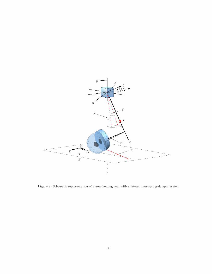
Figure 3: Tyre deformation according to the stretched string tyre model. The turning angle θ is between the directionof motion X and the intersection of the ground and the wheel plane

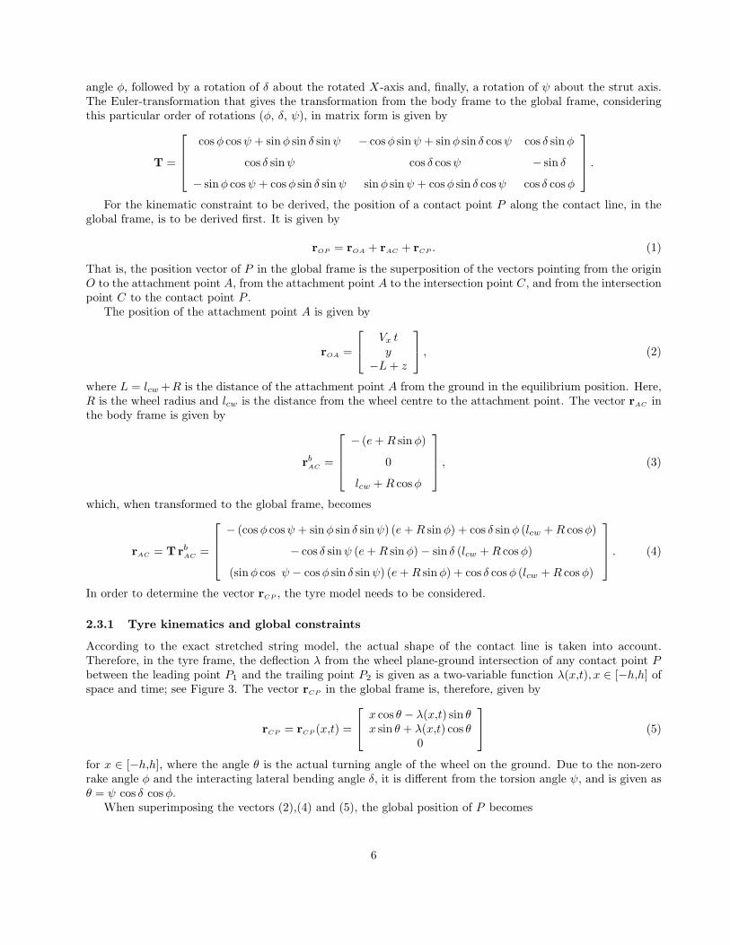
defined as being at 90◦ to the strut – pointing out of the NLG, and η completes the right-handed coordinatesystem. The strut is inclined to the vertical at a fixed rake angle ϕ and allowed to rotate about the body axis ζwith the torsion angle ψ. Moreover, it may rotate in the lateral direction around the body axis ξ as describedby the bending angle δ. Hence, ψ and δ are the two NLG degrees-of-freedom. Further, the strut is modelledas having torsional and lateral stiffnesses and dampings at the attachment point A. Another frame (referredto as the global frame) is fixed to the ground with origin O and axes X,Y and Z. Here, Z is the vertical axispointing downwards, X points in the direction of aircraft motion and Y completes the right-handed coordinatesystem.When ψ = δ = y = 0, that is, in the undisturbed condition, the X-axis is aligned with the central lineof the tyre and A lies in the (X,Z)-plane. The third frame (referred to as the tyre frame) is a local frame usedto describe the tyre deflection; see Figure 3. Its origin is at point C, which is determined as the intersection ofthree intersecting planes. They are the wheel plane, the ground and the plane, that is normal to the ground andincludes the wheel centre point. The axes of the tyre frame are x and λ, where λ is the perpendicular deflectionof the points of the contact line with respect to the wheel plane-ground intersection.

2.3 Kinematics of the coupled system

Rolling without sliding results in a kinematic constraint on the system. In order to derive this constraint thewheel-ground interface is to be considered. It is derived from the assumed condition of the tyre fully adheringto the ground at all times. This means that the absolute velocities of points along the contact line and, inparticular, that of the leading contact point is zero. In order to derive that velocity in terms of the states, thekinematics of the entire system must be analysed.

The motion of the lumped mass is three dimensional translation. It is a combination of the steady-stateforward motion along the X-axis at constant velocity Vx, the harmonic oscillation in the Y -direction and aconstrained vertical motion in the Z-direction; the tyre is assumed to be rigid in radial direction and, hence,as the NLG and the tyre move, the attachment point A must move vertically to maintain ground contact. Themotion of the NLG is genuinely three dimensional. However, since the NLG is suspended by the lumped mass,and the motion relative to the attachment point A is a rotation about a fixed point, the absolute motion can bedescribed by means of relative kinematics. First, the absolute kinematics of the lumped mass and the relativekinematics of the NLG – with respect to the lumped mass – are derived. Then the absolute kinematics of theNLG and, hence, that of the centre of the wheel, can be obtained. Further, by deriving the relative motionof the leading contact point with respect to the wheel plane-ground intersection, the absolute velocity of theleading point and, hence, the required constraint, can be given.

Since the natural frame for the MSD is the global frame, this frame is chosen for the derivations and, therefore,the NLG states must be transformed into the global frame from the moving frame. The instantaneous positionof the NLG and, hence, of the centre of the wheel, with respect to the global frame can be described as theresult of three sequential rotations: a rotation about the Y -axis due to the non-zero but time-independent rake

5

angle ϕ, followed by a rotation of δ about the rotated X-axis and, finally, a rotation of ψ about the strut axis.The Euler-transformation that gives the transformation from the body frame to the global frame, consideringthis particular order of rotations (ϕ, δ, ψ), in matrix form is given by

T =

cosϕ cosψ + sinϕ sin δ sinψ − cosϕ sinψ + sinϕ sin δ cosψ cos δ sinϕ

cos δ sinψ cos δ cosψ − sin δ

− sinϕ cosψ + cosϕ sin δ sinψ sinϕ sinψ + cosϕ sin δ cosψ cos δ cosϕ

.For the kinematic constraint to be derived, the position of a contact point P along the contact line, in the

global frame, is to be derived first. It is given by

rOP = rOA + rAC + rCP . (1)

That is, the position vector of P in the global frame is the superposition of the vectors pointing from the originO to the attachment point A, from the attachment point A to the intersection point C, and from the intersectionpoint C to the contact point P .

The position of the attachment point A is given by

rOA =

Vx ty

−L+ z

, (2)

where L = lcw+R is the distance of the attachment point A from the ground in the equilibrium position. Here,R is the wheel radius and lcw is the distance from the wheel centre to the attachment point. The vector rAC inthe body frame is given by

rbAC =

− (e+R sinϕ)

0

lcw +R cosϕ

, (3)

which, when transformed to the global frame, becomes

rAC = TrbAC =

− (cosϕ cosψ + sinϕ sin δ sinψ) (e+R sinϕ) + cos δ sinϕ (lcw +R cosϕ)

− cos δ sinψ (e+R sinϕ)− sin δ (lcw +R cosϕ)

(sinϕ cos ψ − cosϕ sin δ sinψ) (e+R sinϕ) + cos δ cosϕ (lcw +R cosϕ)

. (4)

In order to determine the vector rCP , the tyre model needs to be considered.

2.3.1 Tyre kinematics and global constraints

According to the exact stretched string model, the actual shape of the contact line is taken into account.Therefore, in the tyre frame, the deflection λ from the wheel plane-ground intersection of any contact point Pbetween the leading point P1 and the trailing point P2 is given as a two-variable function λ(x,t), x ∈ [−h,h] ofspace and time; see Figure 3. The vector rCP in the global frame is, therefore, given by

rCP = rCP (x,t) =

x cos θ − λ(x,t) sin θx sin θ + λ(x,t) cos θ

0

(5)

for x ∈ [−h,h], where the angle θ is the actual turning angle of the wheel on the ground. Due to the non-zerorake angle ϕ and the interacting lateral bending angle δ, it is different from the torsion angle ψ, and is given asθ = ψ cos δ cosϕ.

When superimposing the vectors (2),(4) and (5), the global position of P becomes

6

rOP =

Vxt+ rXAC + x cos θ − λ (x,t) sin θ

y + rYAC + x sin θ + λ (x,t) cos θ

−L+ z + rZAC

, (6)

where rXAC , r

YAC and rZ

AC denote the respective coordinates of (4); they are given by

rX

AC = (cosϕ sinψ − sinϕ sin δ cosψ) (e+R sinϕ) ψ − (sinϕ cos δ sinψ (e+R sinϕ)

+ sin δ sinϕ (lg +R cosϕ)) δ (7)

rY

AC = − cos δ cosψψ (e+R sinϕ) + (sin δ sinψ (e+R sinϕ)− cos δ (lg +R cosϕ)) δ

rZ

AC = − (sinϕ sinϕ+ cosϕ sin δ cosϕ) (e+R sinϕ) ψ − (cosϕ cos δ sinϕ (e+R sinϕ)

+ sin δ cosϕ (lg +R cosϕ)) δ (8)

When differentiated with respect to time, this leads to the velocity of P , that is,

vP = rOP =

Vx + rXAC + x cos θ − x θ sin θ − d

dtλ (x,t) sin θ − λ (x,t) θ cos θ

y + rYAC + x sin θ + x θ cos θ + d

dtλ (x,t) cos θ − λ (x,t) θ sin θz + rZ

AC

. (9)

Here, ddtλ (x,t) is the total derivative of λ (x,t) with respect to time, given by

d

dtλ (x,t) = λ (x,t) + λ′ (x,t) x, (10)

where λ (x,t) and λ′ (x,t) are the partial derivatives with respect to t and x, respectively.The starting point of the derivation was the condition of full tyre adhesion, that is, vP = 0, which leads to

the following scalar constraint equations:

Vx + rX

AC + x cos θ − x θ sin θ −(λ (x,t) + λ′ (x,t) x

)sin θ − λ (x,t) θ cos θ = 0 (11)

y + rY

AC + x sin θ + x θ cos θ +(λ (x,t) + λ′ (x,t) x

)cos θ − λ (x,t) θ sin θ = 0 (12)

z + rZ

AC = 0 (13)

Equation (13) is uncoupled from equations (11) and (12) and it reveals the constraint that governs the verticaldisplacement z of the fuselage. On the other hand, the coupled set of equations (11) and (12) – when solvedfor λ (x,t) – corresponds to the constraint of the lateral displacement of P on the contact line. The solution isa partial differential equation and is given by

λ (x,t) = (Vx + rX

AC) sin θ − (y + rY

AC) cos θ − x θ + λ′ (x,t)(λ (x,t) θ − (Vx + rX

AC) cos θ − (y + rY

AC) sin θ). (14)

However, we are only interested in the lateral displacement of the leading point P1, that is, when x = h. Inthat case, equation (14) can be simplified by the application of the boundary condition

λ′ (x,t)|x=h = −λ1(t)L

. (15)

Therefore, after substitutions, the final form of the constraint equation that describes the kinematics of the tyrebecomes an ordinary differential equation, and is given by

λ (x,t)∣∣∣x=h

= λ1 = (Vx + rX

AC)

(sin θ − λ1

Lcos θ

)− (y + rY

AC)

(cos θ +

λ1L

sin θ

)−(h− λ1

2

L

)θ, (16)

where, for simplicity, λ1 denotes λ1(t). With equations (13) and (16) both constraints are identified.

7

2.4 Equations of motion

During the derivation of the equations of motion, beside the real degrees-of-freedom y, δ and ψ, the verticallumped mass displacement z is taken as a degree-of-freedom too, and the constraint condition (13) is onlyapplied at the final stage. This is done only for more convenient handling of the expressions and has no effecton the final outcome. The different parameters and their values can be found in Table 1.

For each degree-of-freedom the Lagrangian equation

∂

∂t

∂T

∂qi− ∂T

∂qi+∂V

∂qi+∂D

∂qi= Qi (17)

holds, where T is the kinetic energy, V is the potential energy, D is the dissipative energy, Qi is the generalizedforce and qi is the generalized coordinate.

The kinetic energy of the system is

T =1

2µ (vY

A )2 +

1

2M

((vX

A )2 + (vZ

A)2)+

1

2m |vB|2 +

1

2ωB

TJB ωB, (18)

where, vXA , v

YA and vZ

A are the respective global coordinates of the absolute velocity vA of A, vB is the absolutevelocity of B, ωB is the absolute angular velocity of the landing gear and JB is the mass moment of inertiatensor of the NLG at B, in the global frame. Equation (18) is based on the modal mass µ being active only inthe lateral direction, whereas the mass M is active in the forward and vertical directions. Note, that the inertiaeffect of the tyre is not considered and, therefore, the corresponding kinetic energy is zero.

The vector vA is the derivative of (2); it is given by

rOA = vA =

Vx

y

z

. (19)

The absolute velocity of B is the superposition of the absolute velocity of A and the relative velocity of B withrespect to A, that is,

vB = vA + vAB, (20)

wherevAB = ωAB × rAB. (21)

Here, rAB is the relative position of B with respect to A; in the body frame it is given by

rbAB =

0

0

lζ

, (22)

where lζ is the distance from the attachment point A to the centre of gravity B. When transformed to theglobal frame, equation (22) becomes

rAB = TrbAB =

lζ cos δ sinϕ

−lζ sin δ

lζ cos δ cosϕ

. (23)

The vector ωAB in (21) is the relative angular velocity of the NLG with respect to the lumped mass. Sincethere is a sequence of rotations taking place in sequentally rotated body frames, the individual rotation vectorsdo not form an orthogonal set, and so ωAB can only be expressed by superimposing the individual rotationstransformed separately to one of the reference frames. Consequently, the relative angular velocity in the globalframe is given by

8

ωAB =

δ cosϕ+ ψ cos δ sinϕ

−ψ sin δ

−δ sinϕ+ ψ cos δ cosϕ

. (24)

Therefore, after substitutions into (20), the absolute velocity of B becomes

vB =

Vx − δlζ sin δ sinϕ

y − δlζ cos δ

z − δlζ sin δ cosϕ

. (25)

The angular velocity of the MSD is zero; hence, the absolute angular velocity of the landing gear is

ωB = ωAB =

δ cosϕ+ ψ cos δ sinϕ

−ψ sin δ

−δ sinϕ+ ψ cos δ cosϕ

, (26)

and so all terms in equation (18) are determined. The potential energy is

V =1

2kδδ

2 +1

2kψψ

2 +1

2kyy

2, (27)

where kδ, kψ and ky are the respective stiffnesses. The Rayleigh-function for the dissipated energy is given by

D =1

2cδ δ

2 +1

2cψψ

2 +1

2cy y

2, (28)

where cδ, cψ and cy are the respective dampings of the system. After obtaining the equations of motion, theparameters ky and cy are replaced by the natural frequency fn and relative damping q, respectively and, hence,their values are not given.

The generalized forces Qi are calculated from the powers generated by the external, active forces andmoments acting on the system. Those are the gravitational forces GA and GB, given by

GA =

0

0

Mg

, GB =

0

0

mg

, (29)

respectively, and the self aligning moment MKα and lateral tyre force Fy due to the elasticity of the tyre, givenby

MKα =

0

0

−CKαFz

, Fy =

−ΛFz sin θ

ΛFz cos θ

0

, (30)

respectively. Here the coefficients CKα and Λ are given by

CKα =

{kα

αm

π sin(α παm

)if |α| ≤ αm,

0 if |α| > αm,(31)

andΛ = kλ arctan (7.0 tanα) cos (0.95 arctan (7.0 tanα)) , (32)

9

where kλ, kα and αmax are tyre parameters and α=arctan(λ/L) is the slip angle. The original functions of (31)and (32) are defined by Somieski [10] and are both piecewise continuous functions. Although the coefficient(31) is used here in the original form, the piecewise continuous function of (32) has been replaced by a fittedcontinuous function introduced by Thota et al. [12]. As Equations (30) show, both MKα and Fy are functionsof the magnitude Fz of the vertical reaction force Fz at the wheel-ground interface, which is the reaction to theweight and inertia of the system. The vector Fz is given by

Fz =

0

0

−Fz

. (33)

Since the vertical ground constraint (13), is not considered at this stage, the wheel is free to lift off the ground,which can result in loss of contact and, hence, loss of Fz and, consequently, loss of all tyre forces. To avoidthat, and in order to derive the powers generated by the forces and moments, Fz is taken as an independentexternal, active force. This is only necessary due to the derivation method. Once the missing constraint isestablished, Fz becomes the required reaction force. Given the active, external loads and the point of action atC, the powers of Fz, Fy and MKα

are given as

PFz = Fz · vC , (34)

PFy = Fy · vC , (35)

PMKα= MKα · ωB , (36)

respectively. Here, vC is the velocity of C in the global frame; it is given by

vC = vA + vAC , (37)

where vA is the absolute velocity of A – defined by (19) – and vAC is the relative velocity of C with respect toA, given as the derivative of the relative position vector (4). The generalized force, therefore, becomes

Qi =∂PFz

∂qi+∂PFy

∂qi+∂PMKα

∂qi, i ∈ {y, z, δ, ψ}. (38)

After substitutions into (17), for i = y,δ,ψ,z respectively, the set of second-order equations of motion is

(µ+m) y + µ(2qfny + fn

2y)− Cδ δ + Sδ δ

2 − FzΛcos θ = 0, (39)

J1δ + cδ δ + kδδ + J2ψ + 2J3ψδ + J4ψ2 − Cδ y + Sδϕ (g − z) +AδFz = 0, (40)

J5ψ + cψψ + kψψ + J2δ − J3δ2 +AψFz = 0, (41)

(M +m) z − Sδ δ − Cδϕδ2 − (M +m) g + Fz = 0, (42)

whereSδ = mlζ sin δ, Cδ = mlζ cos δ, Sδϕ = mlζ sin δ cosϕ, Cδϕ = mlζ cos δ cosϕ,

and the coefficients Aδ and Aψ are given by

Aδ = (− sin δ sinψ (e+R sinϕ) + cos δ (lcw +R cosϕ)) Λ cos θ − cosϕ cos δ sinψ (e+R sinϕ)

− sin δ cosϕ (lcw +R cosϕ)− (sinϕ cos δ sinψ (e+R sinϕ) + sin δ sinϕ (lcw +R cosϕ)) Λ sin θ

− CKα sinϕ,

Aψ = (cosϕ sinψ − sinϕ sin δ cosψ) (e+R sinϕ) Λ sin θ + cos δ cosψ (e+R sinϕ) Λ cos θ

− (sinϕ sinψ + cosϕ sin δ cosψ) (e+R sinϕ) + CKα cos δ cosϕ.

10

The coefficients J1−J5 are transformed components of the mass moment of inertia tensor of the NLG at B (ξ,η

and ζ are parallel to their body system counterparts ξ,η and ζ)

J1 =(ml2ζ + Jηη

)+(Jξξ − Jηη

)cos2 ψ − Jξη sin (2ψ) , J2 = −Jηζ sinψ + Jξζ cosψ

J3 =(Jηη − Jξξ

)cosψ sinψ − Jξη cos (2ψ) , J4 = −Jξζ sinψ − Jηζ cosψ, J5 = Jζζ .

From equation (42) the expression for Fz can be obtained. It is given by

Fz = (M +m) (g − z) + Sδ δ + Cδϕδ2. (43)

When substituting equation (43) into equations (39)-(41), Fz can be eliminated. Note, that due to not takingthe vertical constraint (13) into account so far, the remaining equations still contain second-order terms of z.However, from the equation (13) z can be obtained as

z = −rZ

AC = Z1δ + Z2δ2 + Z3δψ + Z4ψ

2 + Z5ψ, (44)

where Z1−Z5 are given by

Z1 = cosϕ cos δ sinψ (e+R sinϕ) + sin δ cosϕ (lcw +R cosϕ)

Z2 = − cosϕ sin δ sinψ (e+R sinϕ) + cos δ cosϕ (lcw +R cosϕ)

Z3 = 2 cosϕ cos δ cosψ (e+R sinϕ)

Z4 = (sinϕ cosψ − cosϕ sin δ sinψ) (e+R sinϕ)

Z5 = (sinϕ sinψ + cosϕ sin δ cosψ) (e+R sinϕ)

Therefore, z is eliminated from equations (39)-(41), resulting in the set of equations for y, δ and ψ given by

(µ+m) y + µ(2 q fny + fn

2y)− (Cδ + (Sδϕ − (m+M)Z1) Λ cos θ) δ

+ (Sδ − (Cδϕ − (m+M)Z2) Λ cos θ) δ2 + (m+M)Z3 Λ cos θδψ

+ (m+M)Z4Λ cos (θ) ψ2 + (m+M)Z5Λ cos (θ) ψ − (M +m) gΛ cos θ = 0, (45)

(Aδ (Sδϕ − (m+M)Z1) + J1 − SδϕZ1) δ + (Aδ (Cδϕ − (m+M)Z2)− SδϕZ2) δ2

+ (2 J3 −Aδ (m+M)Z3 − SδϕZ3) δψ + (J4 − SδϕZ4 −Aδ (m+M)Z4) ψ2

+ (J2 −Aδ (m+M)Z5 − SδϕZ5) ψ + (Aδ (M +m) + Sδϕ) g + cδ δ + kδδ − Cδ y = 0, (46)

(J5 −Aψ (m+M)Z5) ψ + (−J3 +Aψ (Cδψ − (m+M)Z2)) δ2 −Aψ (m+M)Z4ψ

2

+ (Aψ (Sδψ − (m+M)Z1) + J2) δ −Aψ (m+M)Z3δψ +Aψ (m+M) g + cpψ + kpψ = 0, (47)

which, along with tyre equation (16), give a complete description of the NLG-fuselage system.

3 Bifurcation analysis

The main focus of the analysis is the interacting lateral fuselage and landing gear dynamics during take-offand landing. In terms of the model this means the study of the conditions for which the trivial straight-rollingsolution [y, ψ, δ]

T= 0 of equations (45)-(47) loses its stability; of interest are also the features of the emerging

11

.

.

.

.

0 0.5 1-60

0

60(a4)

0 0.5 1-3

0

3(a3)

0 10.5-2

0

2(a2)

0 0.5 1-15

0

15(a1)

t [s]

λ[m

m]

y[m

m]

δ[◦

]ψ

[◦]

.

.

0 0.5 1-60

0

60(b4)

0 0.5 1-3

0

3(b3)

0 10.5-2

0

2(b2)

0 0.5 1-15

0

15(b1)

t [s]

λ[m

m]

y[m

m]

δ[◦

]ψ

[◦]

Figure 4: Coexisting torsional (column a) and lateral (column b) oscillations at V = 20m/s, µ = 3t and M = 13t,shown as time series of the variables ψ, δ, y and λ.

12

Parameter Name ValueFuselage datafn natural frequency 2 [Hz]q relative damping 0.02Landing gear datalζ distance from A to B 1.3[m]m mass of the landing gear 320 [kg]

Jζζ m.m. of inertia at B with respect to ζ-axis (axis trough B) 100 [kg m2]

Jξξ

m.m. of inertia. at B with respect to ξ-axis (axis trough B) 100 [kg m2]

Jηη m.m. of inertia at B with respect to η-axis (axis trough B) 100 [kg m2]

Jξη p. of inertia at B with respect to (ξ, η)-axes (axes trough B) 0 [kg m2]

Jξζ

p. of inertia at B with respect to (ξ, ζ)-axes (axes trough B) 0 [kg m2]

Jηζ p. of inertia at B with respect to (η, ζ)-axes (axes trough B) 0 [kg m2]

kδ lateral stiffnes of strut 6.1E6 [Nm rad−1]cδ lateral damping of strut 300 [Nms rad−1]kψ torsional stiffnes of strut 3.8E5 [Nm rad−1]cψ torsional damping of strut 300 [Nms rad−1]lcw distance from point A to the end of the strut 2.138 [m]ϕ rake angle 9 [◦]Tyre and wheel dataR wheel radius 0.362 [m]L relaxation length 0.3 [m]e caster length 0.12 [m]kλ restoring coefficient of the tyre 0.002 [rad−1]h contact patch length 0.1 [m]kα self-aligning coefficient of the tyre 1.0 [m rad−1]αm self-aligning moment limit 10[◦]Otherg gravitational acceleration 9.81 [m s−2]

Table 1: System parameters

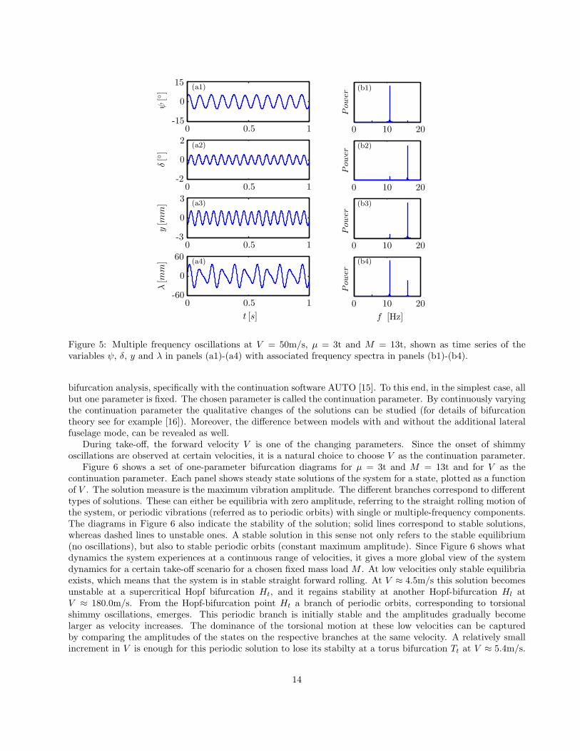
oscillatory behaviour. The aim is to identify parameter regions where the amplitude of the lateral displacementy and its impact on the rest of the system is significant. The equations of motion (45)-(47) with (16) arefully parametrized. They are studied here in terms of changes in the forward velocity V and two structuralparameters: the modal mass µ of the MSD and the vertical mass load M . The parameters of the landing gearare fixed, as well as the natural frequency fn and the relative damping q of the MSD; see Table 1.

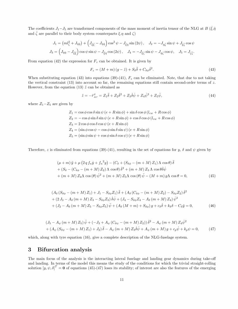
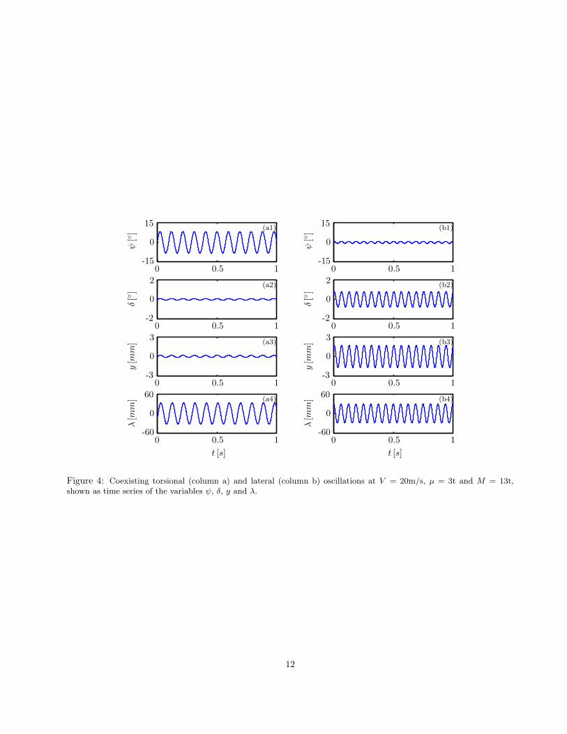
In Figure 4 the result of time simulations of the system at V = 20m/s, µ = 3t and M = 13t is presented.After a transient, the system settles to a stable periodic solution, which is shown in terms of the ψ, δ, y andλ components in Figure 4a. This solution is dominated by oscillations of the torsional angle (with a maximumof ψ ≈ 8◦) and, hence, is also is referred to as torsional shimmy oscillation. The motions of other degrees-of-freedom remain damped, but the dominating oscillation is accompanied by oscillations of both the lateral angleand the lateral fuselage displacement, as well as of the lateral tyre displacement, all at the same frequency off ≈ 10.5Hz. This solution, however, is not unique due to the nonlinearities in the system. Perturbation canmove the system to another stable periodic solution for which the lateral angle is dominant, while the motionsof other degrees-of-freedom follow passively, at the frequency of oscillation of f ≈ 16.0Hz; see Figure 4b. Thissolution is refered to as lateral shimmy oscillation. Figure 5 shows a time series of a stable trajectory forV = 50m/s. Here, the solution contains multiple frequencies, and the dominant one is different for the differentstates; the torsional angle ψ oscillates at close to the torsional frequency of f ≈ 10.8Hz, whereas the lateralstates δ and y oscillate at close to the lateral frequency of f ≈ 16.2Hz. The tyre displacement λ, however,experiences coupled oscillation with two dominant frequencies.

3.1 One-parameter bifurcation analysis

The simulation results show that, for a given set of parameters, different behaviours of the system can beobserved. However, since the behaviour depends on the initial conditions as well it is difficult to investigate allpossible types of behaviour by simulation only. Therefore, the system is analysed further by means of numerical

13

.

.

.

.

0 0.5 1-60

0

60(a4)

0 0.5 1-3

0

3(a3)

0 10.5-2

0

2(a2)

0 0.5 1-15

0

15(a1)

t [s]

λ[m

m]

y[m

m]

δ[◦

]ψ

[◦]

.

.

0 10 20

0 10 20

0 10 20

0 10 20

f [Hz]

Pow

er

Pow

er

Pow

er

Pow

er

(b1)

(b2)

(b3)

(b4)

Figure 5: Multiple frequency oscillations at V = 50m/s, µ = 3t and M = 13t, shown as time series of thevariables ψ, δ, y and λ in panels (a1)-(a4) with associated frequency spectra in panels (b1)-(b4).

bifurcation analysis, specifically with the continuation software AUTO [15]. To this end, in the simplest case, allbut one parameter is fixed. The chosen parameter is called the continuation parameter. By continuously varyingthe continuation parameter the qualitative changes of the solutions can be studied (for details of bifurcationtheory see for example [16]). Moreover, the difference between models with and without the additional lateralfuselage mode, can be revealed as well.

During take-off, the forward velocity V is one of the changing parameters. Since the onset of shimmyoscillations are observed at certain velocities, it is a natural choice to choose V as the continuation parameter.

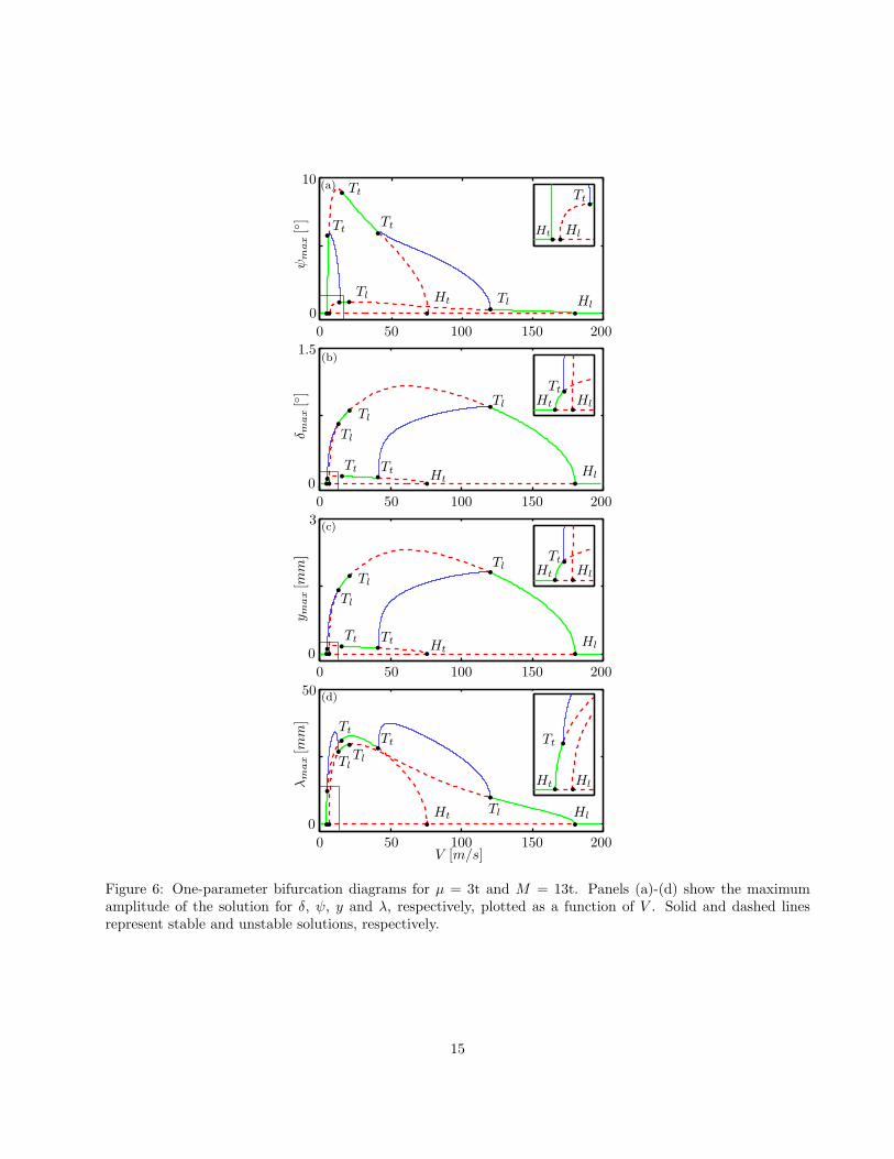
Figure 6 shows a set of one-parameter bifurcation diagrams for µ = 3t and M = 13t and for V as thecontinuation parameter. Each panel shows steady state solutions of the system for a state, plotted as a functionof V . The solution measure is the maximum vibration amplitude. The different branches correspond to differenttypes of solutions. These can either be equilibria with zero amplitude, referring to the straight rolling motion ofthe system, or periodic vibrations (referred as to periodic orbits) with single or multiple-frequency components.The diagrams in Figure 6 also indicate the stability of the solution; solid lines correspond to stable solutions,whereas dashed lines to unstable ones. A stable solution in this sense not only refers to the stable equilibrium(no oscillations), but also to stable periodic orbits (constant maximum amplitude). Since Figure 6 shows whatdynamics the system experiences at a continuous range of velocities, it gives a more global view of the systemdynamics for a certain take-off scenario for a chosen fixed mass load M . At low velocities only stable equilibriaexists, which means that the system is in stable straight forward rolling. At V ≈ 4.5m/s this solution becomesunstable at a supercritical Hopf bifurcation Ht, and it regains stability at another Hopf-bifurcation Hl atV ≈ 180.0m/s. From the Hopf-bifurcation point Ht a branch of periodic orbits, corresponding to torsionalshimmy oscillations, emerges. This periodic branch is initially stable and the amplitudes gradually becomelarger as velocity increases. The dominance of the torsional motion at these low velocities can be capturedby comparing the amplitudes of the states on the respective branches at the same velocity. A relatively smallincrement in V is enough for this periodic solution to lose its stabilty at a torus bifurcation Tt at V ≈ 5.4m/s.

14

.

.

.

.0 50 100 150 200

10

0 r r rr

r

r

r

r r

r

Ht Hl

Tt

Tt

Tt

Tl Tl

.

.

r r

r

Ht Hl

Tt

ψm

ax

[◦]

.

.0 50 100 150 200

0

1.5

r r rrr

r r

r

rr

HtHl

Tt Tt

Tl

Tl

Tl

.

.

r r

r

Ht Hl

Tt

δ max

[◦]

.

.0 50 100 150 200

0

3

r r rrr

r r

r

rr

HtHl

Tt Tt

Tl

Tl

Tl

.

.

r r

r

Ht Hl

Tt

y max

[mm

]

.

.0 50 100 150 200

0

50

r r rr

r

r

rr

r

r

Ht Hl

Tt

Tt

Tl

Tl

Tl

.

.

r r

r

Ht Hl

Tt

V [m/s]

λm

ax

[mm

]

(a)

(b)

(c)

(d)

Figure 6: One-parameter bifurcation diagrams for µ = 3t and M = 13t. Panels (a)-(d) show the maximumamplitude of the solution for δ, ψ, y and λ, respectively, plotted as a function of V . Solid and dashed linesrepresent stable and unstable solutions, respectively.

15

It regains stability at another torus bifurcation Tt at V ≈ 14.6m/s, and then it becomes unstable again at athird torus bifurcation Tt at V ≈ 41.2m/s before the branch bifurcates with the unstable equilibrium at a Hopfbifurcation at V ≈ 75.6m/s. The second branch of periodic solutions emerges from the unstable equilibriumbranch at the Hopf bifurcation Hl at V ≈ 6.5m/s. It is initially unstable but becomes stable when the torusbifurcation Tl at V ≈ 12.9m/s is passed. The solutions along this branch are lateral shimmy oscillations. Thisbranch also becomes unstable at a second torus bifurcation Tl at V ≈ 20.9m/s, but regains stabilty at thetorus bifurcation Tl at V ≈ 120.1m/s. It remains stable until it joins the equlibrium branch at the previouslymentioned Hopf-bifurcation Hl at V ≈ 180.0m/s. There are also two branches of multiple-frequency periodicsolutions (thin solid lines) which connect the two single frequency periodic branches. One emerges from thetorisonal branch at the torus bifurcation Tt at V ≈ 5.4m/s and joins the lateral branch at the torus bifurcationTl at V ≈ 12.9m/s. The other connects the two branches between the torus bifurcations Tt at V ≈ 41.2m/sand Tl at V ≈ 120.1m/s. These branches are calculated by a series of time simulations, since they can notreadily be computed by continuation with AUTO. After identifying a point on the branch by running thesimulation for long enough to get through the transient, the maximum amplitude of the resulting multiple-frequency oscillation is obtained. The next point is then calculated at a different V (sufficiently close to theprevious value) by using the amplitudes of the previous solution as initial conditions for the new simulation.The final curves are interpolated splines, fitted to the obtained sequence of points. The main drawback of thismethod is that only stable branches can be calculated.

In Figure 6 one can follow the dynamics of the system when velocity increases. At low velocities the systemis on the stable equlibrium branch, and so it experiences straight forward rolling. After losing stability atthe first Hopf bifurcation Ht, torsional shimmy oscillation occur. As velocity increases, the amplitude of theoscillations become larger. However, this periodic oscillation too loses stability at the first torus bifurcationTt, beyond which the system is attracted to the first multiple-frequency branch that connects the torsionaland lateral branches. Since between the torus bifurcation points Tt and Tl this branch is the only stable one,the system follows that branch when velocity increases. Close to the torus bifurcation point Tt the torsionalfrequency component is significant; however, the further the velocity moves from Tt the more dominant thelateral component becomes. The dominance of the frequencies and, hence, the observed type of oscillationcompletely exchanges as the branch approaches the periodic branch of lateral solutions. This exchange can beseen in the amplitudes as well. Initially the system experiences torisonal shimmy with a torsional amplitude ofψ ≈ 5◦ and negligible amplitudes of the lateral angle δ and lateral fuselage displacement y amplitudes. However,when moving along the multiple-frequency branch, the torsional amplitude becomes smaller, whereas the lateralamplitudes become larger. After passing the torus bifurcation point Tl, the system experiences single frequencylateral shimmy oscillation. However, since the torsional branch regains stability at V = 14.6m/s and thetorsional branch loses it only at V = 20.9m/s, in between, two stable solutions exist. This means, that the rightperturbation can move the system from one solution to the other. Indeed, Figure 4 shows two such coexistingsolutions in this region. The end of this bistable region is reached with the second torus bifurcation Tl of thelateral branch, where the lateral solution loses stabilty. Passing this point the only remaining stable solutionsare torsional shimmy opscillations and so the system necesserly jumps to them. When that solution too losesstabilty the system is attracted to another multiple-frequency branch, which – being the only stable branch – thesystem follows as velocity increases further, until the branch joins the single frequency lateral periodic branch.The solution shown in Figure 5 is from this region. From that velocity on the system experiences lateral shimmyup to the velocity where the branch bifurcates to the stable equilbrium branch at the Hopf bifurcation Hl. Thevalue of V here, is well outside the range of realistic take-off or landing speeds; nevertheless, continuing thebranches up to these high velocities makes the bifurcation diagrams complete and, hence, helps to understandthe dynamics in the realistic range.

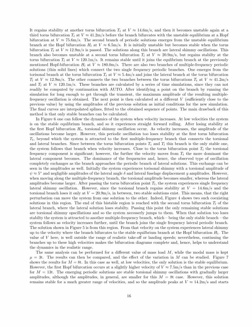
The same analysis can be performed for a different value of mass load M , while the modal mass is keptµ = 3t. The results can then be compared, and the effect of the variation in M can be studied. Figure 7shows the results for M = 8t. In this case as well, at low velocities, the only solution is the stable equilibrium.However, the first Hopf bifurcation occurs at a slightly higher velocity of V ≈ 7.5m/s than in the previous casefor M = 13t. The emerging periodic solutions are stable torsional shimmy oscillations with gradually largeramplitudes, although the amplitudes, in general, are smaller for this M = 8t case. However, this solutionremains stable for a much greater range of velocities, and so the amplitude peaks at V ≈ 14.2m/s and starts

16

.

.

.

.0 50 100 150 200

0

10

r r r r

r

rHl

Tt

.

.

r r

Ht Hl

.

.

r

r

Ht

Tl

ψm

ax

[◦]

.

.0 50 100 150 200

0

1.5

r r r rr

r

r

Ht Hl

Tl

.

.

r r

Ht Hl

.

.

r

r

❄

✻Tt

δ max

[◦]

.

.0 50 100 150 200

0

3

r r r rr

r

r

HtHl

Tl

.

.

r r

Ht Hl

.

.

r

r

❄

✻Tt

y max

[mm

]

.

.0 50 100 150 200

0

50

r r r r

r

r

r

Ht Hl

Tl

.

.

r r

Ht Hl

.

.

r

r❄✻Tt

V [m/s]

λm

ax

[mm

]

(a)

(b)

(c)

(d)

Figure 7: One-parameter bifurcation diagrams for µ = 3t and M = 8t. Panels (a)-(d) show the maximumamplitude of the solution for δ, ψ, y and λ, respectively, plotted as a function of V . Solid and dashed linesrepresent stable and unstable solutons. Arrows denote very steep unstable multiple-frequency branches.

17

.

.0 50 100 150 200

0

10

20

sss ss s s s s sTl Tt Ht Tl Hl

s s s ss s

Ht

Hl

Tt

Ht

Tl

Hl

❇❇◆

s

D

.

.

s s s s sHt Hl

Tl

Tt

Tt

❅❅■

V [m/s]

Stable equlibria

M[t

]

Figure 8: Two-parameter bifurcation diagram in the (V,M)-plane for µ = 3t. Shown are (black) curves of Hopfbifurcation and (grey) curves of torus bifurcation; in the shaded region the straight-rolling solution is stable.The two dashed horizontal lines correspond to Figure 6 and Figure 7 for M = 13t and M = 8t, respectively.The inset is an enlargement around (V,M) = (9, 13).

decreasing afterwards, as can best be seen in Figure 7a. The torsional shimmy oscillation only loses its stabilityat V ≈ 30.6m/s at the torus bifurcation Tt, and at V ≈ 45.9m/s the unstable periodic branch bifurcates withthe unstable equilibrium at the Hopf bifurcation Ht. The second branch of periodic solutions emerges again,from the unstable equilirium branch at the Hopf bifurcation Hl at V ≈ 13.1m/s. This branch is initiallyunstable, becomes stable when the torus bifurcation Tl at V ≈ 49.1m/s is passed and remains stable untiljoining the branch of equlibria at the Hopf bifurcation Hl at V ≈ 84.6m/s. Due to the nature of stable andunstable branches, only one connecting multiple-frequency branch exists. However, the torus bifurcation Tt hereis subcritical, meaning that the branch is initially unstable; it becomes stable very quickly at a velocity onlymarginally higher than that of the torus bifurcation Tt. The stable branch then joins the lateral branch at thetorus bifurcation Tl. These multiple-frequency branches are again obtained by simulation. As discussed earlier,only the stable part of the branches are calculated in this way. Therefore, the unstable branch is representedby double-headed arrows, meaning that only the endpoints of the unstable branch is known, the actual curvein between is not. Notice, that this unstable part of the multiple-frequency branch appears to be very steep.

As Figure 7 shows, variation in the mass load M results in a qualitative change of the bifurcation diagram.ForM = 8t, the torsional solution is dominant for a wider range of velocities, which means that, with increasingvelocity, the system experiences torisonal shimmy oscillations with increasing amplitudes. Then the amplitudereaches a maximum and starts decreasing. Passing the torus bifurcation Tt the only stable branch of solutionsis the multiple-frequency branch. Therefore, the system jumps to that branch and, hence, experiences multiple-frequency oscillations. The dominant oscillation gradually changes from torsional to lateral until it reaches thevelocity of the torus bifurcation Tl, passing of which means that the system again experiences single frequencylateral oscillations. At the Hopf bifurcation Hl, the system returns to the straight forward rolling.

The two cases presented are different not only in terms of the type of single–multiple-frequency transition,but also in terms of the amplitudes and the range of velocities where the equilibrium (no shimmy) solutionis stable. For the case of M = 8t the observed ampitudes are smaller in general, which also means that theconsidered fuselage mode is not excited as much as for M = 13t. On the other hand, the region of stableequilibrium solution is larger, indicating that the mass load has a destabilizing effect on the system; this is inagreement with previous work where the fuselage dynamics are not included; see [12].

18

3.2 Stability diagrams in the (V,M)-plane

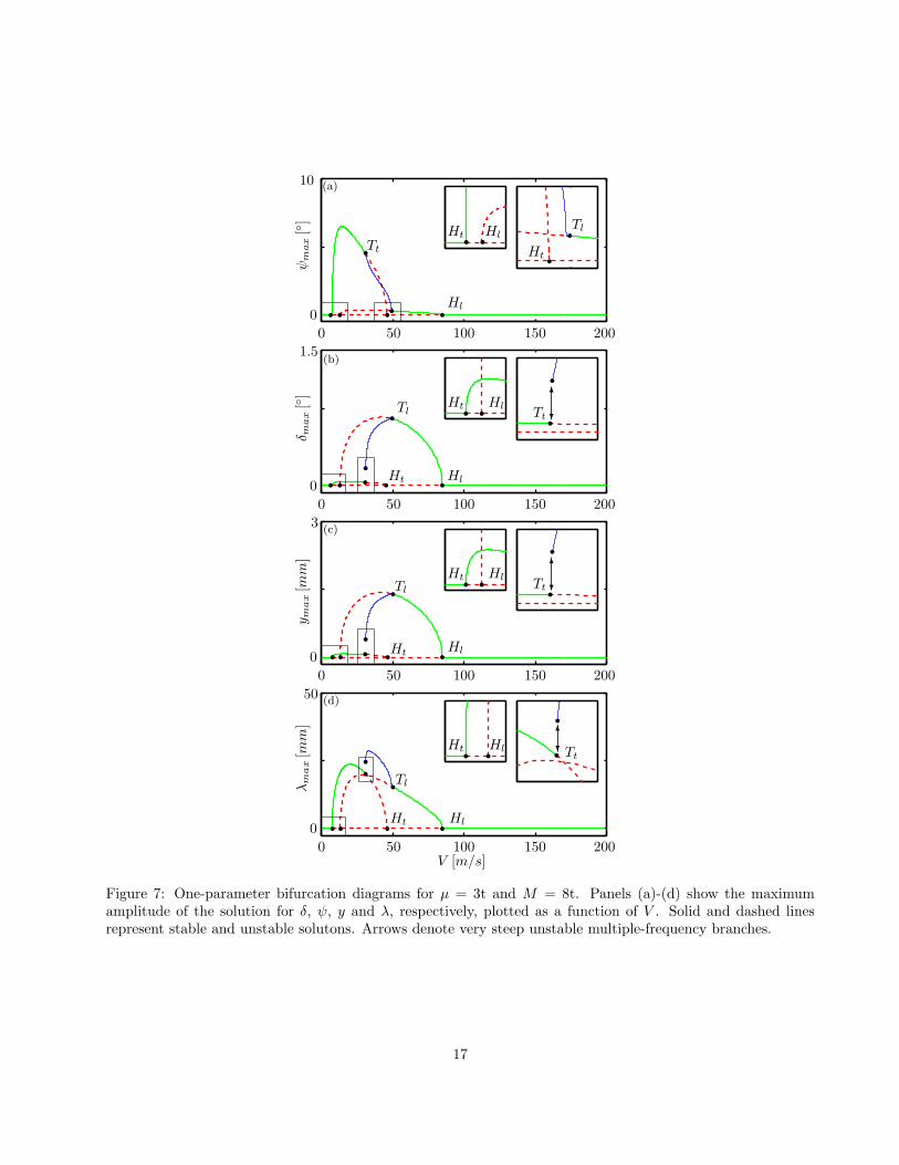
In order to study more thoroughly how the mass load M effects the system, two-parameter continuation isperformed in the continuation parameters V and M . This means that both V and M are now continuouslychanged, for a fixed value of parameter µ. The bifurcation diagram for µ = 3t and for a realistic range of massload M is shown in Figure 8. Horizontal slices of the diagram correspond to one-parameter continuations forfixed mass M , and the red dashed lines correspond to the cases M = 13t and M = 8t in Figures 6 and 7. Thetwo-parameter bifurcation diagram does not show the amplitudes of states, but labels the bifurcation pointsof Figure 6 and Figure 7 along the respective horizontal line. When continuously changing the value of massload M , these bifurcation points generate bifurcation curves: Hopf bifurcation curves, Ht and Hl, and torusbifurcation curves, Tt and Tl, respectively. Further, the two Hopf bifurcation curves intersect at the double Hopfbifurcation point D; two of the four torus bifurcation curves emerge from this point. As Figure 6 and Figure 7show, the stability of the equilibrium solution and, hence, the onset of shimmy oscillations is determined by theHopf-bifurcations. Therefore, the Hopf bifurcation curves in Figure 8 define stability boundaries for the system.The shaded region represents all pairs of V and M , at which the equilibrium solution – corresponding to thestraight-rolling motion – is stable.

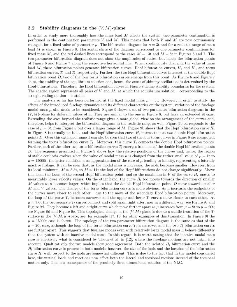
The analysis so far has been performed at the fixed modal mass µ = 3t. However, in order to study theeffects of the introduced fuselage dynamics and its different characterics on the system, variation of the fuselagemodal mass µ also needs to be considered. Figure 9 shows a set of two-parameter bifurcation diagrams in the(V,M)-plane for different values of µ. They are similar to the one in Figure 8, but have an extended M -axis.Extending the axes beyond the realistic range gives a more global view on the arrangement of the curves and,therefore, helps to interpret the bifurcation diagram in the realistic range as well. Figure 9b corresponds to thecase of µ = 3t, from Figure 8 but over a larger range of M . Figure 9b shows that the Hopf bifurcation curve Ht

in Figure 8 is actually an isola, and the Hopf bifurcation curve Hl intersects it at two double Hopf bifurcationpointsD. Over this extended range it can also be seen that two of the four torus curves in Figure 8 are connected,forming the torus bifurcation curve Tt. Moreover, this curve Tt connects the double Hopf bifurcation points.Further, each of the other two torus bifurcation curves Tl emerges from one of the double Hopf bifurcation pointsD. The sequence presented in Figure 9 shows how the relative positions of the curves and, hence, the regionof stable equlibria evolves when the value of modal mass µ is changed from the rather small value of µ = 1t toµ = 15000t; the latter condition is an approximation of the case of µ tending to infinity, representing a laterallyinactive fuslage. It can be seen that, as the modal mass µ increases, the isola becomes smaller. However, fromits local minimum, M ≈ 5.3t, to M ≈ 11t the loci of the Hopf bifurcations do not change significantly. Abovethis load, the locus of the second Hopf bifurcation point, and so the maximum in V of the curve Ht moves tomeasurably lower velocity values. On the other hand, the curve Hl too moves towards the direction of smallerM values as µ becomes larger, which implies that the double Hopf bifurcation points D move towards smallerM and V values. The change of the torus bifurcation curves is more obvious. As µ increases the endpoints ofthe curves move closer to each other – due to the move of the secondary Hopf bifurcation points. Moreover,the loop of the curve Tt becomes narrower and the upper and lower Tl curves move closer to each other. Atµ ≈ 7.6t the two separate Tl curves connect and split again right after, now in a different way; see Figure 9c andFigure 9d. They become a left and a right curve which move further apart as µ increases from µ = 8t to µ = 20t;see Figure 9d and Figure 9e. This topological change in the (V,M)-plane is due to a saddle transition of the Tlsurface in the (V,M, µ)-space; see, for example [17, 18] for other examples of this transition. In Figure 9f theµ = 15000t case is shown. The topology of the two-parameter bifurcation diagram is the same as that of theµ = 20t case, although the loop of the torus bifurcation curve Tt is narrower and the two Tl bifurcation curvesare further apart. This suggests that fuselage modes even with relatively large modal mass µ behave differentlythan the system with an inactive modal mass. In this regard, it is worth noting that the inactive modal masscase is effectively what is considered by Thota et al. in [12], where the fuselage motions are not taken intoaccount. Qualtitatively the two models show good agreement. Both the isolated Ht bifurcation curve and theHl bifurcation curve is present in both models; however, the size of the isola and the location of the bifurcationcurve Hl with respect to the isola are somewhat different. This is due to the fact that in the model consideredhere, the vertical loads and reactions now affect both the lateral and torsional motions instead of the torsionalmotion only. This is a consequence of the genuinely three-dimensional rotation of the NLG.

19

.

.

.

.0 50 100 150 200

0

10

20

30

40

50

V [m/s]

Stable equlibria

M[t

]

s

s

D

D

TlTt

Ht

Hl

.

.0 50 100 150 200

0

10

20

30

40

50

V [m/s]

Stable equlibria

M[t

]

s

s

D

D

TlTt

Ht

Hl

.

.0 50 100 150 200

0

10

20

30

40

50

V [m/s]

Stable equlibria

M[t

]

s

s

D

DTl

Tt

Ht

Hl

.

.0 50 100 150 200

0

10

20

30

40

50

V [m/s]

Stable equlibria

M[t

]

s

s

D

DTl

Tt

Ht

Hl

Tl

❄

.

.0 50 100 150 200

0

10

20

30

40

50

V [m/s]

Stable equlibria

M[t

]

s

s

D

D TlTt

Ht

Hl

Tl

✁✁☛

.

.0 50 100 150 200

0

10

20

30

40

50

V [m/s]

Stable equlibria

M[t

]

s

s

D

D TlTt

Ht

Hl

Tl

✂✂✌

(a) (b)

(c) (d)

(e) (f)

Figure 9: Two-parameter bifurcation diagrams in the (V,M)-plane for µ = 1t (a), µ = 3t (b), µ = 6t (c), µ = 8t(d), µ = 20t (e) and µ = 15000t (to approximate an infinitely large modal mass) (f). Shown are (black) curvesof Hopf bifurcation and (light) curves of torus bifurcation; in the shaded region the straight-rolling solution isstable.

20

3.3 Stability diagrams in the (V, µ)-plane

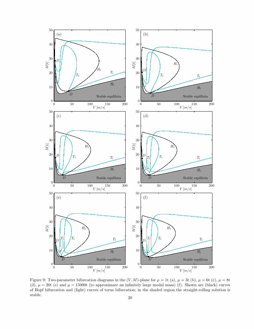
As discussed in Section 3.2, not only do the bifurcation diagrams in the (V,M)-plane show how changes inthe modal mass µ affect the stability of the system, but the case approximating the inactive mass makes theconnection with previous work [12] as well. Figure 9 also reveals that, due to the changing topology of thetorus bifurcation curves Tt and Tl, the number of changes in the stability of the periodic solutions, and thevelocities at which those happen, is affected by the variation of µ. However, the selected distinct values of µ donot appear to significantly affect the region of stable equlibria. In order to obtain a more general understandingof the dynamics related to the introduced fuselage dynamics, and to identify modal mass µ values, where theeffect on the stable equilibria is significant, a second two-parameter analysis is performed, this time in V and µfor fixed values of M . A sequence of bifurcation diagrams in the (V, µ)-plane is shown in Figure 10, where thepanels correspond to different fixed M values between M = 7t and M = 15t. Here, all panels are composedof the same curves as those of Figure 9, although they are shown from a different perspective. The connectionbetween Figure 10 and Figure 9 is made by the horizontal slices of different panels; i.e. the slice taken at µ = 3tin Figure 10a represents dynamics for the same parameters as that taken at M = 7t in Figure 9b.

Figure 10a shows the bifurcation diagram for M = 7t. The isolated Hopf bifurcation curve Ht of Figure 9now manifests itself as two separate curves Ht, while the Hopf bifurcation curve Hl is connected in the (V, µ)-plane as well. Again, the curves Ht and Hl intersect at the double Hopf bifurcation point D and a pair of torusbifurcation curves, Tt and Tl emerge from the these points. Due to the fact that there are now two curves Ht,the region of stable equilibrium solutions now consists of two components. The sequence of panels in Figure 10shows how the arrangement changes due to the variation of the load M . As M increases, the region of stableequlibria shrinks. This is due to the descending curve Hl, but also to the fact that the curves Ht move furtherapart; this corresponds to the widening of the isola in Figure 9. The joint relocation of the curves also resultsin different locations of the double Hopf bifurcation point D and the appearing of another intersection point Din the region of interest when M = 15t; see Figure 10f. Further, the shape of the two torus bifurcation curvesTt and Tl changes significantly. The monotone curves in Figure 10a start to have local minima and maximafor larger values of M ; see Figure 10b and Figure 10c. As M increases, the local minima and maxima movetowards smaller and larger values of µ, respectively. Moreover, the maxima of the curves gradually move out ofthe region of interest; see Figure 10c and Figure 10d. The position of the minima are of importance in terms ofthe dynamics of the system, because they define critical values of modal mass, below which stable branches ofperiodic solutions appear or disappear.

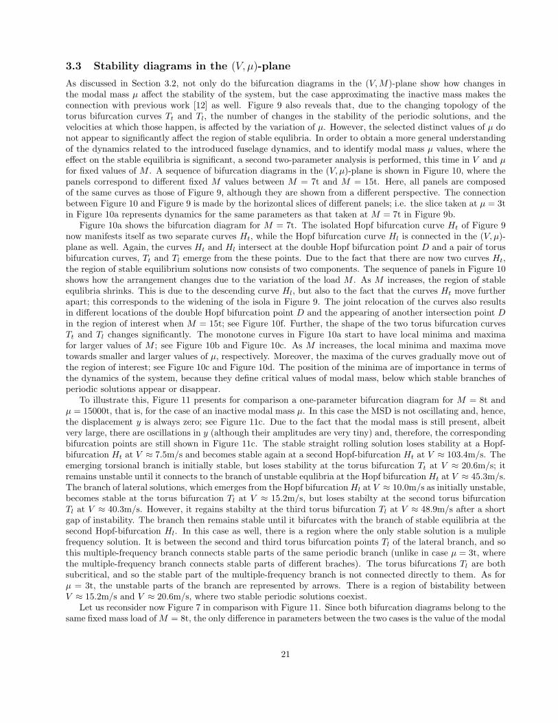
To illustrate this, Figure 11 presents for comparison a one-parameter bifurcation diagram for M = 8t andµ = 15000t, that is, for the case of an inactive modal mass µ. In this case the MSD is not oscillating and, hence,the displacement y is always zero; see Figure 11c. Due to the fact that the modal mass is still present, albeitvery large, there are oscillations in y (although their amplitudes are very tiny) and, therefore, the correspondingbifurcation points are still shown in Figure 11c. The stable straight rolling solution loses stability at a Hopf-bifurcation Ht at V ≈ 7.5m/s and becomes stable again at a second Hopf-bifurcation Ht at V ≈ 103.4m/s. Theemerging torsional branch is initially stable, but loses stability at the torus bifurcation Tt at V ≈ 20.6m/s; itremains unstable until it connects to the branch of unstable equlibria at the Hopf bifurcationHt at V ≈ 45.3m/s.The branch of lateral solutions, which emerges from the Hopf bifurcationHl at V ≈ 10.0m/s as initially unstable,becomes stable at the torus bifurcation Tl at V ≈ 15.2m/s, but loses stabilty at the second torus bifurcationTl at V ≈ 40.3m/s. However, it regains stabilty at the third torus bifurcation Tl at V ≈ 48.9m/s after a shortgap of instability. The branch then remains stable until it bifurcates with the branch of stable equilibria at thesecond Hopf-bifurcation Hl. In this case as well, there is a region where the only stable solution is a muliplefrequency solution. It is between the second and third torus bifurcation points Tl of the lateral branch, and sothis multiple-frequency branch connects stable parts of the same periodic branch (unlike in case µ = 3t, wherethe multiple-frequency branch connects stable parts of different braches). The torus bifurcations Tl are bothsubcritical, and so the stable part of the multiple-frequency branch is not connected directly to them. As forµ = 3t, the unstable parts of the branch are represented by arrows. There is a region of bistability betweenV ≈ 15.2m/s and V ≈ 20.6m/s, where two stable periodic solutions coexist.

Let us reconsider now Figure 7 in comparison with Figure 11. Since both bifurcation diagrams belong to thesame fixed mass load ofM = 8t, the only difference in parameters between the two cases is the value of the modal

21

.

.

.

.0 50 100 150 200

0

5

10

15

20

V [m/s]

Stable equilibra

µ[t

]

s

D

Hl

Ht

Ht

Tl

Tt

❄

.

.0 50 100 150 200

0

5

10

15

20

s

D

Hl

Ht

Ht

Tl

Tt

V [m/s]

Stable equilibra

µ[t

]

.

.0 50 100 150 200

0

5

10

15

20

V [m/s]

Stable equilibra

µ[t

]

s

D

Hl

Ht

Ht

Tl

Tl

Tt

.

.0 50 100 150 200

0

5

10

15

20

V [m/s]

Stable equilibra

µ[t

]

s

D❆❆❯

Hl

Ht

Ht

Tl

Tl

Tt

✄✄✗

❈❈❈❈❈❖

.

.0 50 100 150 200

0

5

10

15

20

V [m/s]

Stable equilibra

µ[t

]

s

D

HlHt

Ht

Tl

Tl

Tt

Tt

✏✏✮

✄✄✄✎

.

.0 50 100 150 200

0

5

10

15

20

V [m/s]

S. e.

µ[t

]

s

DHl

Ht

Ht

✛¡¡

Tl

Tl

Tt

Tt

❈❈❈❲

(a) (b)

(c) (d)

(e) (f)

Figure 10: Two-parameter bifurcation diagrams in the (V, µ)-plane for M = 7t (a), M = 7.8t (b), M = 8t (c),M = 9t (d), M = 12t (e) and M = 15t (f). Shown are (black) curves of Hopf bifurcation and (light) curves oftorus bifurcation; in the shaded regions the straight-rolling solution is stable.

22

.

.

.

.0 50 100 150 200

0

10

rr r r

r

rr r

r

Tl Hl

Tt

.

.

r r

Ht Hl

.

.

r

r r

r

Tl Tl

Ht

❄✻

❳❳

ψm

ax

[◦]

.

.0 50 100 150 200

0

1.5

rr r rr

r

r

r rr

Ht HlTt

Tl

.

.

r r

Ht Hl

.

.

r

r

r

rTl

Tl

❄✻❄✻

δ max

[◦]

.

.0 50 100 150 200

0

3

rr r rr rr rr

y max

[mm

]

.

.0 50 100 150 200

0

50

rr r r

r

rrr

r

Ht Hl

Tt

Tl

.

.

r r

Ht Hl

.

.

r

r

r

r

Tl Tl

❄✻

❄✻

V [m/s]

λm

ax

[mm

]

(a)

(b)

(c)

(d)

Figure 11: One-parameter bifurcation diagrams for µ = 15000t and M = 8t. The large µ value represents aninactive modal mass. Panels (a)-(d) show the maximum amplitude of the solution for δ, ψ, y and λ, respectively,plotted as a function of V . Solid and dashed lines represent stable and unstable solutons, respectively. Arrowsdenote very steep unstable multiple-frequency branches.

23

mass µ. Therefore, the changes that an active modal mass may cause in the behaviour of the NLG-fuselagesystem compered to the inactive case, can be studied. One obvious difference between Figure 7 and Figure 11is the activated oscillations of the MSD and, hence, of its lateral displacement y. A second change, consideringthis particular modal mass case of µ = 3t, is the disappearence of the first stable region from the lateral branch.This means that the bistable region disappears as well and, consequently, the multiple-frequency branch nowconnects the lateral brach with the torsional branch instead of connecting the same lateral branch. Also, thetorus bifurcation Tt on the torsional branch moved to a higher velocity in Figure 7 whereas the second Hopfbifurcation Hl moved to a lower velocity. These changes have a dual effect on the dynamics. The first is thatbetween V ≈ 20.6m/s and V ≈ 40.3m/s, where the only stable solution is the lateral solution in the inactivecase, the stable solutions are now either the torisonal solution (V ≈ 20.6− 30.6m/s) or the multiple-frequencysolution (V ≈ 30.6−40.3m/s); hence, in this region the lateral shimmy oscillations are now changed to torsionalshimmy oscillations or multiple-frequency oscillations. Moreover, due to the relocation of the Hopf bifurcationHl, the region where the straight-rolling solution is stable is smaller.

The differences between the one-parameter bifurcation diagrams, Figure 7 and Figure 11, can be explainedby the two-parameter bifurcation diagram of Figure 10c. All are for the case M = 8t and the one-parameterbifurcation diagrams are horizontal slices of the two-parameter bifurcation diagram. The µ = 15000t case iswell out of the range of Figure 10c, but it is effectively approximated as the highest available mass load value ofµ = 20t, because the locations of the curves do not change significantly above that value of µ; see also Figure 9eand Figure 9f. As can be seen in Figure 10c, the reason for the loss of stability of the torsional branch occuringat a higher velocity is that the torus bifurcation curve Tt moves towards higher velocities. Also, the lack of thestable lateral solution in Figure 7 between V ≈ 15.2 − 40.3m/s is due to the fact, that the loop of the torusbifurcation curve Tl, which bounds a region of stable lateral solutions, has a minimum at µ ≈ 7.4t. The loopsof torus bifurcation curves Tt and Tt, therefore, are of great importance as – for a fixed value of mass load –they define limit values of modal mass µ, where the existence of stable solutions changes. The comparison ofFigures 7 and 11 clearly reveals that the laterally active mass can have a significant influence on the systemdynamics – depending on its modal properties and the value of the load.

4 Conclusions

Based on an established NLG model, an extended NLG-fuselage model was presented to model the interactionbetween those two sub-systems. The NLG model has two degrees of freedom: the torsion angle ψ and the lateralbending angle δ, and takes into account the general three-dimensional motion that the NLG is exposed to whilemoving on the runway. The fuselage is modelled by a linear second-order mass-spring-damper system with onelateral degree-of-freedom y. Consequently, fuselage modes with lateral component were considered here. Thisfuselage model – as well as the landing gear model – is fully parametrized, and so the modal characteristicsof the considered mode can be changed. The tyre is modelled by the exact stretched string model. Althoughthe overall model is capable of handling changes in all the parameters, we focused here on changes in three ofthem: the forward velocity V , the vertical mass load M , and the modal mass µ of the fuselage. In terms of thefuselage model it means that the natural frequency is set to a fixed value, and the modal properties are variedby changing the value of the modal mass µ only.

The main question of the study was at what modal mass values the landing gear can excite the consideredfuselage mode and, moreover, when this interaction is significant. To this end, numerical bifurcation analysiswas used and one- and two-parameter bifurcation diagrams were presented to demonstrate how the systembehaviour depends on the chosen parameters. It was found, that, due to the strong coupling between thesub-systems, the landing gear can trigger vibrations in the fuselage. The amplitude and frequency of thoseoscillations strongly depend on the modal mass of the fuselage. This means that, given the right parameters,fuselage modes having lateral components can be excited during take-off and landing. Moreover, it was shownthat a significant proportion of the excitation energy feeds modes of lower modal masses. By comparing alaterally inactive mass to an oscillating one, it was demonstrated that the fuselgage dynamics and its couplingto the landing gear have an influence on the landing gear dynamics; therefore, the extended model can improvepredictions of shimmy oscillations in aircrafts.

24

Overall, it was shown that the model presented here is sufficient for demonstrating that significant interactionis possible between the nose landing gear and a lateral fuselage mode as represented by a mass-spring-dampersystem. In particular, a real-time dynamic substructuring test appears to be feasible. The next step towardsimplementing such a hybrid test would be to introduce the dynamics of the actuators and to identify controlparameters at which the system is stable. The NLG-fuselage model presented considers a linear, one degree-of-freedom model of a simple fuselage mode. Moreover, the fuselage characterics were changed with the modalmass, while the natural frequency was kept fixed. A next step would be to vary the natural frequency as well.A longer term goal would be a full study of the dynamic effects of an aircraft fuselage, as it is connected tothe ground via the nose landing gear as well as the main landing gears; such work would require considerablefurther extensions of the present model.

Acknowledgement: The authors thank Sanjiv Sharma, Etienne Coetzee, Phanikrishna Thota and Peter Hart(Airbus in the UK) for helpful discussions and their support. The research of Nandor Terkovics was supportedby the Engineering and Physical Sciences Research Council (EPSRC) in collaboration with Airbus in the UK.

References

[1] B. von Schlippe and R. Dietrich. Shimmying of a pneumatic wheel. Technical Report NACA TM 1365,National Advisory Committee for Aeronautics, 1947.

[2] Hans B. Pacejka. The wheel shimmy phenomenon: a theoretical and experimental investigation with par-ticular reference to the nonlinear problem. Phd thesis, Delft University of Technology, 1966.

[3] Hans B. Pacejka. Analysis of the shimmy phenomenon. In Proceedings of the Institution of MechanicalEngineers, volume 180.1, pages 251–268, 1965.

[4] Hans B. Pacejka. Tyre and Vehicle Dynamics. Butterworth-Heinemann, second edition, 2006.

[5] L. Segel. Force and moment response of pneumatic tires to lateral motion inputs. ASME, Transactions,Journal of Engineering for Industry, 88:37–44, 1966.

[6] G. Stepan. Delay, nonlinear oscillations and shimmying wheels. In New applications of nonlinear andchaotic dynamics in mechanics, pages 373–386. Kluwer Academic Publisher, 1999.

[7] D. Takacs, G. Orosz, and G. Stepan. Delay effects in shimmy dynamics of wheels with stretched string-liketyres. European Journal of Mechanics A/Solid, 28:516–525, 2009.

[8] D. Takacs and G. Stepan. Experiments on quasiperiodic wheel shimmy. Journal of Computational andNonlinear Dynamics, 4:031007–1, 2009.

[9] R. F. Smiley. Correlation, evaluation, and extension of linearized theories for tyre motion and wheelshimmy. Technical Report 1299, National Advisory Committee for Aeronautics, 1957.

[10] G. Somieski. Shimmy analysis of a simple aircraft nose landing gear model using different mathematicalmethods. Aerospace Science and Technology, 1(8):545–555, 1997.

[11] P. Thota, B. Krauskopf, and M. Lowenberg. Shimmy in a non-linear model of an aircraft nose landing gearwith nonzerorake angle. In Proceedings of ENOC, 2008.

[12] P. Thota, B. Krauskopf, and M. Lowenberg. Interaction of torsion and lateral bending in aircraft noselanding gear shimmy. Nonlinear Dynamics, 57(3), 2009.

[13] O.S. Bursi and D.J. Wagg. Real-time testing with dynamic substructuring. In Modern Testing Techniquesfor Structural Systems, pages 293–342. Springer, 2008.

25

[14] A. Blakeborough, M. S. Williams, A. P. Darby, and D. M. Williams. The development of real-time sub-structure testing. Philosophical Transactions of the Royal Society of London A, 359:1869–1891, 2001.

[15] E. J Doedel, H. B Keller, and J. P Kernevez. Numerical analysis and control of bifurcation problems, partii: bifurcation in infinite dimensions. Int J Bifurcat Chaos Appl Sci Eng, 1(4):745–772, 1991.

[16] Yuri A. Kuznetsov. Elements of Applied Bifurcation Theory. Springer, 1995.

[17] P. Thota, B. Krauskopf, and M. Lowenberg. Multi-parameter bifurcation study of shimmy oscillation in adual-wheel aircraft nose landing gear. Nonlinear Dynamics, 70(2):1675–1688, 2012.

[18] H. Erzgraber, B. Krauskopf, and D. Lenstra. Bifurcation analysis of a semiconductor laser with filteredoptical feedback. SIAM Journal on Applied Dynamical Systems, 6.1:1–28, 2007.

26