Biclustering meets Triadic Concept AnalysisBiclustering meets Triadic Concept Analysis Mehdi Kaytoue Sergei O. Kuznetsov Juraj Macko Amedeo Napoli Received: date / Accepted: date Abstract

Noname manuscript No.(will be inserted by the editor)

Biclustering meets Triadic Concept Analysis

Mehdi Kaytoue · Sergei O. Kuznetsov ·Juraj Macko · Amedeo Napoli

Received: date / Accepted: date

Abstract Biclustering numerical data became a popular data-mining task atthe beginning of 2000’s, especially for gene expression data analysis and recom-mender systems. A bicluster reflects a strong association between a subset ofobjects and a subset of attributes in a numerical object/attribute data-table.So-called biclusters of similar values can be thought as maximal sub-tables withclose values. Only few methods address a complete, correct and non-redundantenumeration of such patterns, a well-known intractable problem, while no for-mal framework exists. We introduce important links between biclustering andFormal Concept Analysis (FCA). Indeed, FCA is known to be, among others,a methodology for biclustering binary data. Handling numerical data is notdirect, and we argue that Triadic Concept Analysis (TCA), the extension ofFCA to ternary relations, provides a powerful mathematical and algorithmicframework for biclustering numerical data. We discuss hence both theoreticaland computational aspects on biclustering numerical data with triadic conceptanalysis. These results also scale to n-dimensional numerical datasets.

Keywords numerical biclustering · similarity relation · formal conceptanalysis · triadic concept analysis · n-ary relations

Mehdi KaytoueUniversite de Lyon, CNRS, INSA-Lyon, LIRIS, UMR5205, F-69621, FranceE-mail: [email protected]

Sergei O. KuznetsovHigher School of Economis (HSE) – Pokrovskiy Bd. 11 – 109028 Moscow – RussiaE-mail: [email protected]

Juraj MackoPalacky University – 17. listopadu – 77146 Olomouc – Czech RepublicE-mail: [email protected]

Amedeo NapoliLaboratoire Lorrain de Recherche en Informatique et ses Applications (LORIA)Campus Scientifique, B.P. 239, F-54500 Vandœuvre-les-Nancy, FranceE-mail: [email protected]

2 Mehdi Kaytoue et al.

1 Introduction

Taking roots in the work of Hartigan [13] in 1972 and extended by Mirkin in1996 [27], numerical data biclustering then strongly attracted attention fromthe beginning of 2000’s as a first answer to new challenges raised by gene ex-pression data analysis [11] and recommender systems design [1]. Starting froman object/attribute numerical data-table, the goal is to group together someobjects with some attributes according to the values taken by these attributesfor these objects. The main idea of biclustering is to overcome the limitation ofstandard clustering techniques producing partitions of objects where distancefunctions that use all the attributes may be ineffective and hard to inter-pret [2]. For example, in gene expression data, it is known that genes (objects)may share a common behavior for a subset of biological situations (attributes)only: one should accordingly produce local patterns to characterize biologicalprocesses, the latter should possibly overlap, since a gene may be involved inseveral processes. The same remark applies for recommender systems, wherethe taste of users for some items is realized by a so-called utility matrix (usu-ally very sparse): one is interested in local patterns characterizing groups ofusers that strongly share almost the same tastes for a subset of items [1].

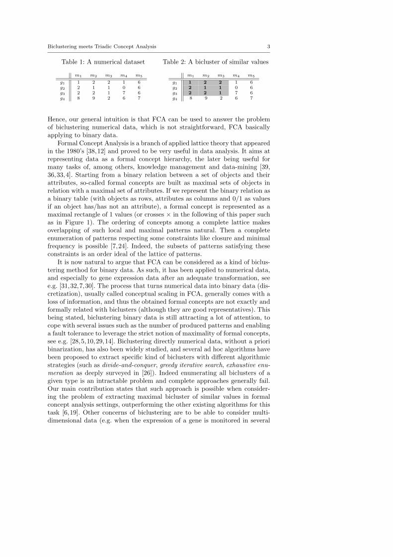
Accordingly, a bicluster is formally defined as a pair composed of a setof objects and a set of attributes. Such a pair can be represented as a rect-angle in a numerical table, modulo rows and columns permutations. Table 1is a numerical dataset with objects in rows and attributes in columns, whileeach table entry corresponds to the value taken by the attribute in columnfor the object in row. Table 2 illustrates bicluster ({g1, g2, g3}, {m1,m2,m3})as a grey rectangle that can be understood as a sub-table of the original one.There are several types of biclusters in the literature, depending on the relationbetween the values taken by their attributes for their objects (as surveyed byMadeira and Oliveira [26]). The most simple case can be understood as rectan-gles of equal values: a bicluster corresponds to a set of objects whose attributestake exactly the same value, e.g. ({g1, g2, g3}, {m5}). Constant biclusters onlyappear in idyllic situations. Accordingly, a straightforward generalization ofsuch biclusters lies in so-called biclusters of similar values: they are repre-sented by rectangles with almost identical, say similar, values (see [26,6,19]and to a similar extent [9]). Table 2 illustrates a bicluster of similar values({g1, g2, g3}, {m1,m2,m3}) where two values are said to be similar if theirdifference is no more than 1. Moreover, this bicluster is maximal: neither anobject nor an attribute can be added without violating the similarity condi-tion. The problem of biclustering that we investigate in this paper consists inextracting all pairs (A,B), such that A and B are maximal sets with respectto a similarity constraint between values.

To better understand our investigation, we recall a definition of bicluster ofPrelic et al. in binary data or relation, i.e. an object has or not an attribute [32]:inclusion-maximal biclusters are defined as maximal sets of objects related toa maximal set of attributes. As shown in [21], this definition exactly meets theone of formal concepts in the Formal Concept Analysis theory (FCA, [12]).

Biclustering meets Triadic Concept Analysis 3

Table 1: A numerical dataset

m1 m2 m3 m4 m5

g1 1 2 2 1 6g2 2 1 1 0 6g3 2 2 1 7 6g4 8 9 2 6 7

Table 2: A bicluster of similar values

m1 m2 m3 m4 m5

g1 1 2 2 1 6g2 2 1 1 0 6g3 2 2 1 7 6g4 8 9 2 6 7

Hence, our general intuition is that FCA can be used to answer the problemof biclustering numerical data, which is not straightforward, FCA basicallyapplying to binary data.

Formal Concept Analysis is a branch of applied lattice theory that appearedin the 1980’s [38,12] and proved to be very useful in data analysis. It aims atrepresenting data as a formal concept hierarchy, the later being useful formany tasks of, among others, knowledge management and data-mining [39,36,33,4]. Starting from a binary relation between a set of objects and theirattributes, so-called formal concepts are built as maximal sets of objects inrelation with a maximal set of attributes. If we represent the binary relation asa binary table (with objects as rows, attributes as columns and 0/1 as valuesif an object has/has not an attribute), a formal concept is represented as amaximal rectangle of 1 values (or crosses × in the following of this paper suchas in Figure 1). The ordering of concepts among a complete lattice makesoverlapping of such local and maximal patterns natural. Then a completeenumeration of patterns respecting some constraints like closure and minimalfrequency is possible [7,24]. Indeed, the subsets of patterns satisfying theseconstraints is an order ideal of the lattice of patterns.

It is now natural to argue that FCA can be considered as a kind of biclus-tering method for binary data. As such, it has been applied to numerical data,and especially to gene expression data after an adequate transformation, seee.g. [31,32,7,30]. The process that turns numerical data into binary data (dis-cretization), usually called conceptual scaling in FCA, generally comes with aloss of information, and thus the obtained formal concepts are not exactly andformally related with biclusters (although they are good representatives). Thisbeing stated, biclustering binary data is still attracting a lot of attention, tocope with several issues such as the number of produced patterns and enablinga fault tolerance to leverage the strict notion of maximality of formal concepts,see e.g. [28,5,10,29,14]. Biclustering directly numerical data, without a prioribinarization, has also been widely studied, and several ad hoc algorithms havebeen proposed to extract specific kind of biclusters with different algorithmicstrategies (such as divide-and-conquer, greedy iterative search, exhaustive enu-meration as deeply surveyed in [26]). Indeed enumerating all biclusters of agiven type is an intractable problem and complete approaches generally fail.Our main contribution states that such approach is possible when consider-ing the problem of extracting maximal bicluster of similar values in formalconcept analysis settings, outperforming the other existing algorithms for thistask [6,19]. Other concerns of biclustering are to be able to consider multi-dimensional data (e.g. when the expression of a gene is monitored in several


situations across time [40,35]) and parallelization of the algorithms [8] whichboth are important issues we address in this paper. This leads us to our maincontributions.

Problem. We consider here maximal biclusters of similar values, denotedby (A,B) where A and B are respectively maximal sets of objects and at-tributes, such that the values taken by these attributes for these objects arepairwise similar. Given a similarity parameter θ, the similarity relation is de-fined as a 'θ b ⇐⇒ |b− a| ≤ θ, for any numbers a and b. The problem is todesign an approach that allows an exact, correct and complete extraction ofmaximal biclusters of similar values.

Contribution 1. Triadic Concept Analysis (TCA) [25] is an extension ofFCA to handle ternary relations: an object has an attribute under a givencondition. This leads to triadic contexts, i.e. data are represented as a ”box”,where so-called triadic concepts can be seen as maximal sets of objects inrelation with a maximal set of attributes under a maximal set of conditions,i.e. a maximal ”sub-box” of × in the context (still with rows, columns andlayers permutations). We show then, that after turning the original numer-ical data in a triadic context without loss of information (with interordinalscaling [12]), the resulting triadic concepts are in 1-1-correspondence with themaximal biclusters of similar values for any similarity parameter θ (statingif two values are similar or not). Then, such concepts can be organized in atrilattice whose diagram gives a visualization of biclusters in the numericaldataset. Finally, we show that this result naturally holds when consideringn-dimensional numerical datasets.

Contribution 2. Maximal biclusters of similar values for a user-definedsimilarity parameter have been studied with complete approaches in [6,19]. In[6], an algorithm for extracting such biclusters is presented, while [19] showshow such biclusters can be characterized by post-processing a concept latticebuilt from the numerical data directly. We show that our first contributioncan be easily adapted to answer this problem, with a new generic algorithmTriMax that shows better results than its competitors and can be naturallyparallelized.

For summarizing, this research article is two-fold: first, theoretical newlinks are emphasized between biclustering and FCA in general, and TCA inparticular, for a better understanding of numerical pattern mining with closureoperators. Secondly, a computational aspect is investigated using these links:it allows one to bring back a problem of biclustering into well known-settings(i.e. FCA and pattern-mining) and comes with better computational propertiesand several perspectives of research. Note that this paper paper extends ourprevious work [18] by adapting the methodology to n-dimensional data andshowing how the set of concepts can be represented by line diagrams.

The paper is organized as follows. Firstly, we present the preliminariesregarding FCA and TCA in Section 2. Thanks to the introduced notations, weformally state the problem in Section 3. The sections 4,5 respectively tackle ourtwo main contributions. The paper ends with a conclusion suggesting furtherresearch.


2 Formal Concept Analysis

Formal Concept Analysis (FCA) [12] is a mathematical framework for allowingone to derive implicit relationships from a set of objects and their attributes.Starting from a relation stating which objects have which attributes, it allowsone to build a so-called concept lattice. A concept is there seen as a maximalset of objects sharing a maximal set of attributes. Ordering concepts witha specialization/generalization relation gives rise to a concept lattice. Thisstructure can be represented by a diagram where classes of objects/attributesand ordering relations between classes can be drawn, interpreted and used fordata-mining, knowledge management and discovery [36,39].

2.1 Dyadic concept analysis

We use standard definitions from [12]. Let G and M be arbitrary sets and I ⊆G×M be an arbitrary binary relation between G and M . The triple (G,M, I)is called a formal context, or dyadic context. Each g ∈ G is interpreted asan object, each m ∈ M is interpreted as an attribute. The fact (g,m) ∈ I isinterpreted as “g has attribute m”. The two following derivation operators (·)′:

A′ = {m ∈M | ∀g ∈ A : gIm} for A ⊆ G,B′ = {g ∈ G | ∀m ∈ B : gIm} for B ⊆M

define a Galois connection between the powersets of G and M . The derivationoperators {(·)′, (·)′} put in relation elements of the lattices (℘(G),⊆) of ob-jects and (℘(M),⊆) of attributes and vice-versa. A Galois connection inducesclosure operators (·)′′ and realizes a one-to-one correspondence between allclosed sets of objects and all closed sets of attributes. For A ⊆ G, B ⊆ M ,a pair (A,B) such that A′ = B and B′ = A, is called a formal concept, ordyadic concept. Concepts are partially ordered by (A1, B1) ≤ (A2, B2)⇔ A1 ⊆A2 (⇔ B2 ⊆ B1). (A1, B1) is a sub-concept of (A2, B2), while the latter is asuper-concept of (A1, B1). With respect to this partial order, the set of all for-mal concepts forms a complete lattice called the concept lattice of the formalcontext (G,M, I), i.e. any subset of concepts has both a supremum (join) andan infimum (meet), see Theorem 1. For a concept (A,B) the set A is calledthe extent and the set B the intent of the concept.

Theorem 1 (The Basic Theorem on Concept Lattices [12]) The con-cept lattice of a context (G,M, I) is a complete lattice in which infimum andsupremum are given by:

∧t∈T

(At, Bt) =

(⋂t∈T

At,

(⋃t∈T

Bt

)′′)∨t∈T

(At, Bt) =

((⋃t∈T

At

)′′,⋂t∈T

Bt

)


m1 m2 m3

g1 ×g2 × ×g3 × ×g4 × ×

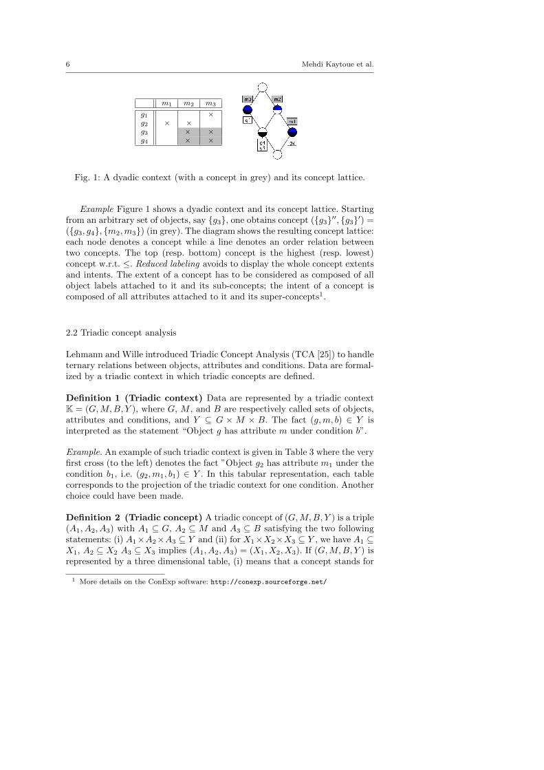
Fig. 1: A dyadic context (with a concept in grey) and its concept lattice.

Example Figure 1 shows a dyadic context and its concept lattice. Startingfrom an arbitrary set of objects, say {g3}, one obtains concept ({g3}′′, {g3}′) =({g3, g4}, {m2,m3}) (in grey). The diagram shows the resulting concept lattice:each node denotes a concept while a line denotes an order relation betweentwo concepts. The top (resp. bottom) concept is the highest (resp. lowest)concept w.r.t. ≤. Reduced labeling avoids to display the whole concept extentsand intents. The extent of a concept has to be considered as composed of allobject labels attached to it and its sub-concepts; the intent of a concept iscomposed of all attributes attached to it and its super-concepts1.

2.2 Triadic concept analysis

Lehmann and Wille introduced Triadic Concept Analysis (TCA [25]) to handleternary relations between objects, attributes and conditions. Data are formal-ized by a triadic context in which triadic concepts are defined.

Definition 1 (Triadic context) Data are represented by a triadic contextK = (G,M,B, Y ), where G, M , and B are respectively called sets of objects,attributes and conditions, and Y ⊆ G × M × B. The fact (g,m, b) ∈ Y isinterpreted as the statement “Object g has attribute m under condition b”.

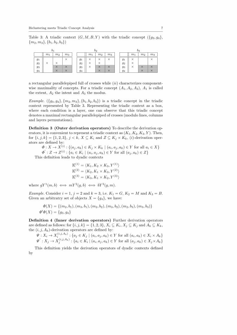
Example. An example of such triadic context is given in Table 3 where the veryfirst cross (to the left) denotes the fact ”Object g2 has attribute m1 under thecondition b1, i.e. (g2,m1, b1) ∈ Y . In this tabular representation, each tablecorresponds to the projection of the triadic context for one condition. Anotherchoice could have been made.

Definition 2 (Triadic concept) A triadic concept of (G,M,B, Y ) is a triple(A1, A2, A3) with A1 ⊆ G, A2 ⊆ M and A3 ⊆ B satisfying the two followingstatements: (i) A1×A2×A3 ⊆ Y and (ii) for X1×X2×X3 ⊆ Y , we have A1 ⊆X1, A2 ⊆ X2 A3 ⊆ X3 implies (A1, A2, A3) = (X1, X2, X3). If (G,M,B, Y ) isrepresented by a three dimensional table, (i) means that a concept stands for

1 More details on the ConExp software: http://conexp.sourceforge.net/


Table 3: A triadic context (G,M,B, Y ) with the triadic concept ({g3, g4},{m2,m3}, {b1, b2, b3})

b1 b2 b3m1 m2 m3

g1 ×g2 × ×g3 × ×g4 × ×

m1 m2 m3

g1 × × ×g2 × ×g3 × × ×g4 × ×

m1 m2 m3

g1 × ×g2 ×g3 × × ×g4 × ×

a rectangular parallelepiped full of crosses while (ii) characterizes component-wise maximality of concepts. For a triadic concept (A1, A2, A3), A1 is calledthe extent, A2 the intent and A3 the modus.

Example. ({g3, g4}, {m2,m3}, {b1, b2, b3}) is a triadic concept in the triadiccontext represented by Table 3. Representing the triadic context as a box,where each condition is a layer, one can observe that this triadic conceptdenotes a maximal rectangular parallelepiped of crosses (modulo lines, columnsand layers permutations).

Definition 3 (Outer derivation operators) To describe the derivation op-erators, it is convenient to represent a triadic context as (K1,K2,K3, Y ). Then,for {i, j, k} = {1, 2, 3}, j < k, X ⊆ Ki and Z ⊆ Kj ×Kk, (i)-derivation oper-ators are defined by:

Φ : X → X(i) : {(aj , ak) ∈ Kj ×Kk | (ai, aj , ak) ∈ Y for all ai ∈ X}Φ

′: Z → Z(i) : {ai ∈ Ki | (ai, aj , ak) ∈ Y for all (aj , ak) ∈ Z}

This definition leads to dyadic contexts

K(1) = 〈K1,K2 ×K3, Y(1)〉

K(2) = 〈K2,K1 ×K3, Y(2)〉

K(3) = 〈K3,K1 ×K2, Y(3)〉

where gY 1(m, b) ⇐⇒ mY 2(g, b) ⇐⇒ bY 3(g,m).

Example. Consider i = 1, j = 2 and k = 3, i.e. K1 = G, K2 = M and K3 = B.Given an arbitratry set of objects X = {g4}, we have:

Φ(X) = {(m2, b1), (m3, b1), (m2, b2), (m3, b2), (m2, b3), (m3, b3)}Φ′Φ(X) = {g3, g4}

Definition 4 (Inner derivation operators) Further derivation operatorsare defined as follows: for {i, j, k} = {1, 2, 3}, Xi ⊆ Ki, Xj ⊆ Kj and Ak ⊆ Kk,the (i, j, Ak)-derivation operators are defined by:

Ψ : Xi → X(i,j,Ak)i : {aj ∈ Kj | (ai, aj , ak) ∈ Y for all (ai, ak) ∈ Xi×Ak}

Ψ′

: Xj → X(i,j,Ak)j : {ai ∈ Ki | (ai, aj , ak) ∈ Y for all (aj , ak) ∈ Xj×Ak}

This definition yields the derivation operators of dyadic contexts definedby


KijAk= 〈Ki,Kj , Y

ijAk〉

where (ai, aj) ∈ Y ijAk⇐⇒ ai, aj , ak are related by Y for all ak ∈ Ak

Example. Consider i = 1, j = 2 and k = 3, i.e. K1 = G, K2 = M and K3 = B,A3 = {b1, b2} and X = {g3}:

Ψ(X) = {m2,m3} Ψ ′Ψ(X) = {g3, g4}

Operators Φ and Φ′

are called outer operators, a composition of both opera-tors is called outer closure. Operators Ψ and Ψ

′are called inner operators, a

composition of them is called inner closure.

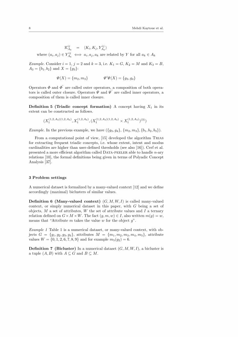
Definition 5 (Triadic concept formation) A concept having X1 in itsextent can be constructed as follows.

(X(1,2,A3)(1,2,A3)1 , X

(1,2,A3)1 , (X

(1,2,A3)(1,2,A3)1 ×X(1,2,A3)

1 )(3))

Example. In the previous example, we have ({g3, g4}, {m2,m3}, {b1, b2, b3}).

From a computational point of view, [15] developed the algorithm Triasfor extracting frequent triadic concepts, i.e. whose extent, intent and moduscardinalities are higher than user-defined thresholds (see also [16]). Cerf et al.presented a more efficient algorithm called Data-peeler able to handle n-aryrelations [10], the formal definitions being given in terms of Polyadic ConceptAnalysis [37].

3 Problem settings

A numerical dataset is formalized by a many-valued context [12] and we defineaccordingly (maximal) biclusters of similar values.

Definition 6 (Many-valued context) (G,M,W, I) is called many-valuedcontext, or simply numerical dataset in this paper, with G being a set ofobjects, M a set of attributes, W the set of attribute values and I a ternaryrelation defined on G×M×W . The fact (g,m,w) ∈ I, also written m(g) = w,means that “Attribute m takes the value w for the object g”.

Example 1 Table 1 is a numerical dataset, or many-valued context, with ob-jects G = {g1, g2, g3, g4}, attributes M = {m1,m2,m3,m4,m5}, attributevalues W = {0, 1, 2, 6, 7, 8, 9} and for example m5(g2) = 6.

Definition 7 (Bicluster) In a numerical dataset (G,M,W, I), a bicluster isa tuple (A,B) with A ⊆ G and B ⊆M .


Definition 8 (Similarity relation and bicluster of similar values) Letw1, w2 ∈ W be two attribute values and θ ∈ R be a user-defined parameter,called similarity parameter or threshold. w1 and w2 are said to be similar iff|w1 − w2| ≤ θ, which we denote by w1 'θ w2. (A,B) is bicluster of similarvalues if m(g) 'θ n(h) for all g, h ∈ A and for all m,n ∈ B.

Definition 9 (Maximal bicluster of similar values) A bicluster of similarvalues (A,B) is maximal if adding either an object in A or an attribute in Bdoes not result in a bicluster of similar values.

Example 2 (From Table 1) ({g1, g4}, {m2,m4}) is a bicluster. ({g1, g2}, {m2})is a bicluster of similar values with θ ≥ 1. However, it is not maximal. With1 ≤ θ < 5, ({g1, g2, g3}, {m1,m2,m3}) is maximal. Finally, with θ = 7 thebicluster ({g1, g2, g3}, {m1,m2,m3,m4,m5}) is maximal. Note that a constant(maximal) bicluster is a (maximal) bicluster of similar values with θ = 0.

Thus the problem that we address in this article is the extraction of allmaximal biclusters of similar values from a numerical dataset. We desire theextraction to be complete, correct and non-redundant compared to most ofexisting methods of the literature based on heuristics [26]. We will show thatFCA is a good candidate as a formal framework for such a task.

4 Biclusters of similar values in Triadic Concept Analysis

This first contribution considers the problem of generating maximal biclustersfor any θ with TCA after a scaling procedure. We then show how to representthe resulting set of concepts with line diagrams, and extend the methodologyto n-dimensional numerical datasets.

4.1 Scaling numerical data into a triadic context

Starting from a numerical dataset (G,M,W, I), the basic idea lies in buildinga triadic context (G,M, T, Y ) where the two first dimensions remain formalobjects and formal attributes, while W is scaled into a third dimension denotedby T . This new dimension T is called the scale dimension: intuitively, it givesdifferent “spaces of values” that each object-attribute pair (g,m) ∈ G ×Mcan take. Once the scale is given, a triadic context is derived and it gives riseto triadic concepts.

We use the interordinal scaling [12] to build the scale dimension. It allowsone to encode in 2T all possible intervals of values in W . This scale allowsone to derive a triadic context from which any bicluster of similar values canbe characterized as a triadic concept. We make these statements more preciseand illustrate the whole procedure with examples.

Definition 10 (Interordinal Scaling) A scale is a binary relation J ⊆W ×T associating original elements from the set of values W to their derived


J t 1=

[0,0]

t 2=

[0,1]

t 3=

[0,2]

t 4=

[0,6]

t 5=

[0,7]

t 6=

[0,8]

t 7=

[0,9]

t 8=

[1,9]

t 9=

[2,9]

t 10=

[6,9]

t 11=

[7,9]

t 12=

[8,9]

t 13=

[9,9]

0 × × × × × × ×1 × × × × × × ×2 × × × × × × ×6 × × × × × × ×7 × × × × × × ×8 × × × × × × ×9 × × × × × × ×

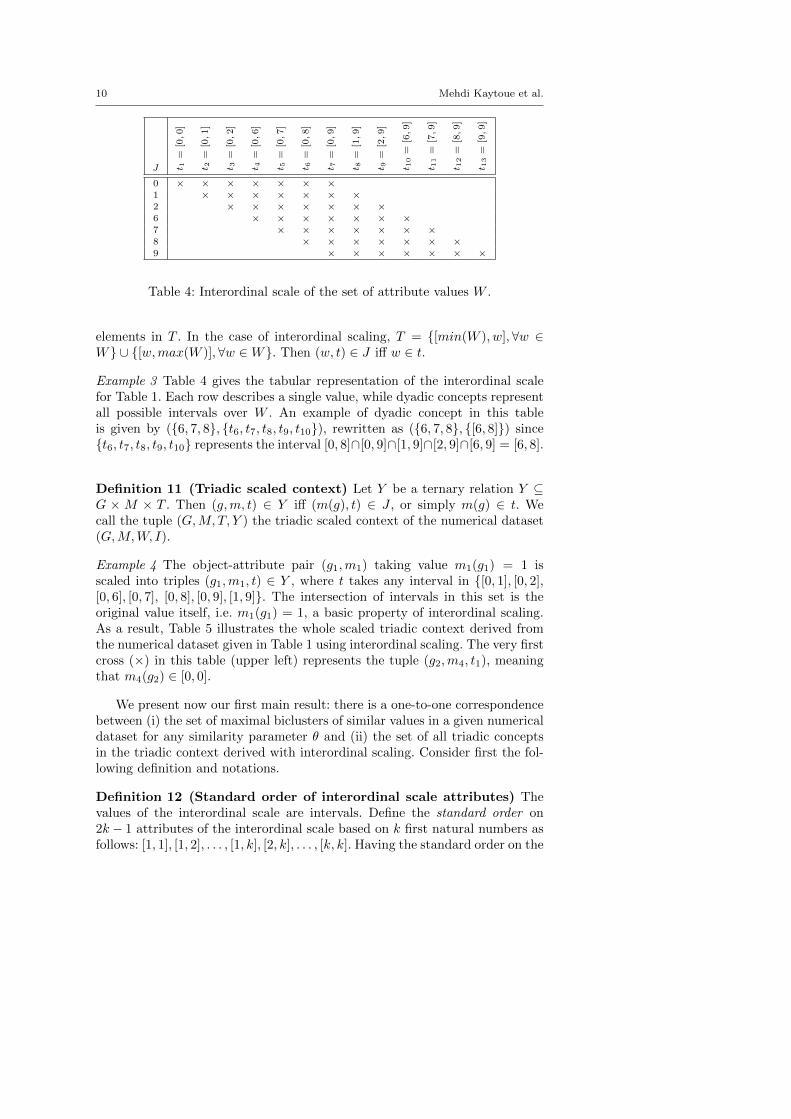
Table 4: Interordinal scale of the set of attribute values W .

elements in T . In the case of interordinal scaling, T = {[min(W ), w],∀w ∈W} ∪ {[w,max(W )],∀w ∈W}. Then (w, t) ∈ J iff w ∈ t.

Example 3 Table 4 gives the tabular representation of the interordinal scalefor Table 1. Each row describes a single value, while dyadic concepts representall possible intervals over W . An example of dyadic concept in this tableis given by ({6, 7, 8}, {t6, t7, t8, t9, t10}), rewritten as ({6, 7, 8}, {[6, 8]}) since{t6, t7, t8, t9, t10} represents the interval [0, 8]∩[0, 9]∩[1, 9]∩[2, 9]∩[6, 9] = [6, 8].

Definition 11 (Triadic scaled context) Let Y be a ternary relation Y ⊆G × M × T . Then (g,m, t) ∈ Y iff (m(g), t) ∈ J , or simply m(g) ∈ t. Wecall the tuple (G,M, T, Y ) the triadic scaled context of the numerical dataset(G,M,W, I).

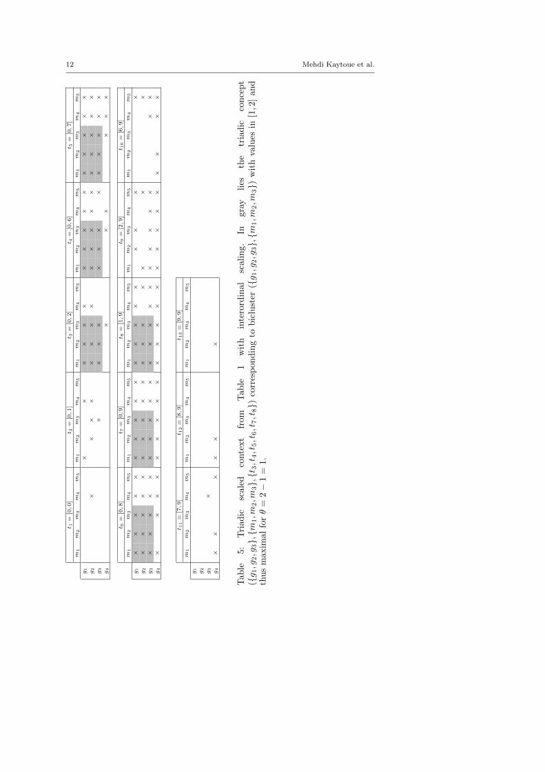
Example 4 The object-attribute pair (g1,m1) taking value m1(g1) = 1 isscaled into triples (g1,m1, t) ∈ Y , where t takes any interval in {[0, 1], [0, 2],[0, 6], [0, 7], [0, 8], [0, 9], [1, 9]}. The intersection of intervals in this set is theoriginal value itself, i.e. m1(g1) = 1, a basic property of interordinal scaling.As a result, Table 5 illustrates the whole scaled triadic context derived fromthe numerical dataset given in Table 1 using interordinal scaling. The very firstcross (×) in this table (upper left) represents the tuple (g2,m4, t1), meaningthat m4(g2) ∈ [0, 0].

We present now our first main result: there is a one-to-one correspondencebetween (i) the set of maximal biclusters of similar values in a given numericaldataset for any similarity parameter θ and (ii) the set of all triadic conceptsin the triadic context derived with interordinal scaling. Consider first the fol-lowing definition and notations.

Definition 12 (Standard order of interordinal scale attributes) Thevalues of the interordinal scale are intervals. Define the standard order on2k − 1 attributes of the interordinal scale based on k first natural numbers asfollows: [1, 1], [1, 2], . . . , [1, k], [2, k], . . . , [k, k]. Having the standard order on the


attributes of the interordinal scale one can think of attributes having numbersfrom 1 to 2k + 1. Note the obvious main property of the standard order onattributes of the interordinal scale: if an object has two scale attributes withnumbers r and s, r < s, then it has all scale attributes with numbers in [r, s].

For a many-valued context (G,M,W, I), let the set W (|W | = q) be the setof numerical values enumerated in the ascending order from 1 to q, and let g(m)be a map taking attribute m to its value w ∈W for object g. Let the numericalvalues from W be interordinally scaled with the standard order on the scaleattributes, so we can denote the scale attributes by m1, . . . ,mq, . . . ,m2q−1. LetB = {m1, . . . ,mq, . . .m2q−1} and (G,M,B, Y ) be the triadic context such that(g,m, b) ∈ Y iff g(m) lies in the interval given by the interordinal attribute b.

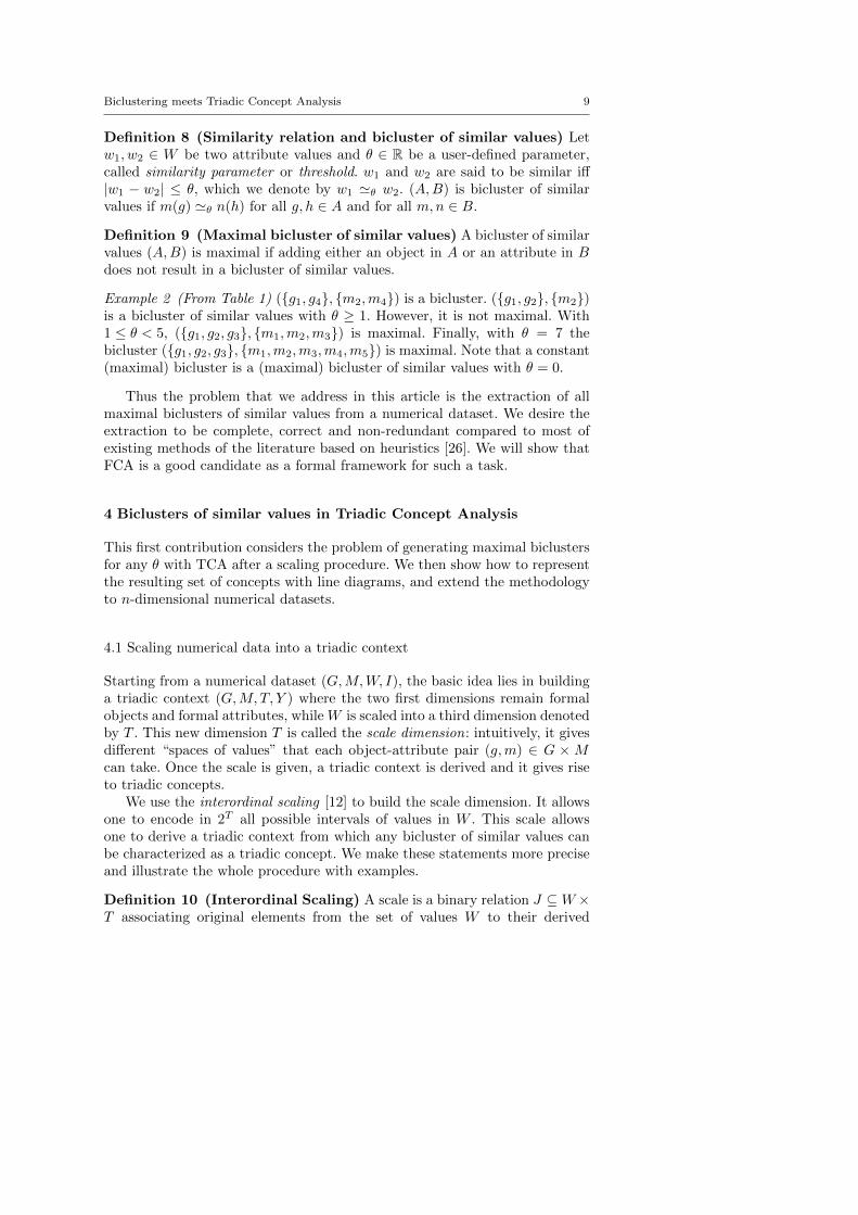
Proposition 1 (A,D) is a maximal bicluster of similar values (A ⊆ G, D ⊆M) with the values lying in the interval [t, t+θ] for t ∈ N, θ ≥ 0 iff (A,D,U) isa triadic concept of the context (G,M,B, Y ) , where U = {t+θ, . . . q, . . . , q+t−1}. Moreover, every triadic concept of the interordinally scaled triadic context(G,M,B, Y ) is of the form (A,D,U), where A ⊆ G,D ⊆ M , and U = {t +θ, . . . q, . . . , q + t− 1} for some t ∈ N and θ ≥ 0.

Proof Let (A,D) be a maximal bicluster of similar values (A ⊆ G, D ⊆M), then the values of attributes of the bicluster are lying in the interval[t, t + θ] for some t ∈ N, θ ≥ 0, i.e. g(m) ∈ [t, t + θ] for every g ∈ A, m ∈ D.Due to the standard order on interordinal attributes, this implies that in thetriadic context (G,M,B, Y ) one has (g,m, b) ∈ Y for all g ∈ A,m ∈ Dand b ∈ {t + θ, . . . q, . . . , q + t − 1} and there is a rectangular parallelepiped(A,D, {t+θ, . . . q, . . . , q+ t−1}) filled with crosses in the triadic cross-table ofY , i.e. (A,D, {t+ θ, . . . q, . . . , q + t− 1} ⊆ Y . This parallelepiped is inclusion-maximal, since otherwise this would mean that one can add either anotherobject, or another attribute, or another scale value to its respective component.The possibility of adding another object or attribute would contradict the factthat (A,D) is a maximal bicluster, the possibility of adding another scale valuewould contradict the fact that the attribute values of the bicluster lie strictlyin the interval [t, t + θ] . Thus, (A,D, {t + θ, . . . q, . . . , q + t − 1}) is a triadicconcept.

In the opposite direction, consider a triadic concept (A,D, V ) in the in-terordinally scaled three-dimensional context, the attributes of V being or-dered in the standard way. By the main property of the standard order onattributes of the interordinal scale, this would mean that for any two valuesr and s of V , the set V also contains all values in the interval [r, s]. Hencethere are some t and q such that the values of V lie in the interval [t, t+ θ] forall object-attribute pairs from A × D. This means that (A,D) is a biclusterof similar values, which is maximal, since otherwise (A,D, V ) would not havebeen a triadic concept.

Example 5 ({g1, g2, g3}, {m1,m2,m3}, {t3, t4, t5, t6, t7, t8}) is a triadic conceptcorresponding to the maximal bicluster ({g1, g2, g3}, {m1,m2,m3}) with θ = 1since {t3, t4, t5, t6, t7, t8} is a modus characterizing interval [1, 2] of length 1.

12 Mehdi Kaytoue et al.t 1

=[0,0]

t 2=

[0,1]

t 3=

[0,2]

t 4=

[0,6]

t 5=

[0,7]

m1

m2

m3

m4

m5

m1

m2

m3

m4

m5

m1

m2

m3

m4

m5

m1

m2

m3

m4

m5

m1

m2

m3

m4

m5

g1

××

××

××

××

××

××

××

××

g2

××

××

××

××

××

××

××

××

××

g3

××

××

××

××

××

××

×g4

××

××

××

t 6=

[0,8]

t 7=

[0,9]

t 8=

[1,9]

t 9=

[2,9]

t 10=

[6,9]

m1

m2

m3

m4

m5

m1

m2

m3

m4

m5

m1

m2

m3

m4

m5

m1

m2

m3

m4

m5

m1

m2

m3

m4

m5

g1

××

××

××

××

××

××

××

××

××

×g2

××

××

××

××

××

××

××

××

×g3

××

××

××

××

××

××

××

××

××

××

××

g4

××

××

××

××

××

××

××

××

××

××

××

×

t 11=

[7,9]

t 12=

[8,9]

t 13=

[9,9]

m1

m2

m3

m4

m5

m1

m2

m3

m4

m5

m1

m2

m3

m4

m5

g1

g2

g3

×g4

××

××

××

Tab

le5:

Tri

adic

scal

edco

nte

xt

from

Tab

le1

wit

hin

tero

rdin

al

scali

ng.

Ingra

yli

esth

etr

iad

icco

nce

pt

({g 1,g

2,g

3},{m

1,m

2,m

3},{t

3,t

4,t

5,t

6,t

7,t

8})

corr

esp

on

din

gto

bic

lust

er({g 1,g

2,g

3},{m

1,m

2,m

3})

wit

hva

lues

in[1,2

]an

dth

us

max

imal

forθ

=2−

1=

1.


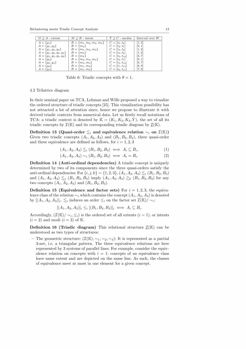
G ⊇ A - extent M ⊇ B - intent T ⊇ C - modus Interval over W

A = {g1} B = {m1,m2,m3,m4} C = [t3, t8] [1, 2]A = {g1, g2} B = {m4} C = [t2, t7] [0, 1]A = {g1, g2, g3} B = {m1,m2,m3} C = [t3, t8] [1, 2]A = {g1, g2, g3, g4} B = {m3} C = [t3, t8] [1, 2]A = {g1, g2, g3, g4} B = {m5} C = [t5, t10] [6, 7]A = {g2} B = {m2,m3,m4} C = [t2, t7] [0, 1]A = {g3, g4} B = {m4,m5} C = [t5, t10] [6, 7]A = {g4} B = {m1,m2} C = [t7, t12] [8, 9]A = {g4} B = {m1,m5} C = [t6, t11] [7, 8]

Table 6: Triadic concepts with θ = 1.

4.2 Trilattice diagram

In their seminal paper on TCA, Lehman and Wille proposed a way to visualizethe ordered structure of triadic concepts [25]. This visualization possibility hasnot attracted a lot of attention since, hence we propose to illustrate it withderived triadic contexts from numerical data. Let us firstly recall notations ofTCA: a triadic context is denoted by K = (K1,K2,K3, Y ), the set of all itstriadic concepts by I(K) and its corresponding triadic diagram by I(K).

Definition 13 (Quasi-order .i and equivalence relation ∼i on I(K))Given two triadic concepts (A1, A2, A3) and (B1, B2, B3), three quasi-orderand three equivalence are defined as follows, for i = 1, 2, 3

(A1, A2, A3) .i (B1, B2, B3) ⇐⇒ Ai ⊆ Bi, (1)

(A1, A2, A3) ∼i (B1, B2, B3) ⇐⇒ Ai = Bi. (2)

Definition 14 (Anti-ordinal dependencies) A triadic concept is uniquelydetermined by two of its components since the three quasi-orders satisfy theanti-ordinal dependencies: For {i, j, k} = {1, 2, 3}, (A1, A2, A3) .i (B1, B2, B3)and (A1, A2, A3) .j (B1, B2, B3) imply (A1, A2, A3) &k (B1, B2, B3) for anytwo concepts (A1, A2, A3) and (B1, B2, B3).

Definition 15 (Equivalence and factor sets) For i = 1, 2, 3, the equiva-lence class of the relation∼i which contains the concept (A1, A2, A3) is denotedby [(A1, A2, A3)]i. .i induces an order ≤i on the factor set I(K)/ ∼i:

[(A1, A2, A3)]i ≤i [(B1, B2, B3)]i ⇐⇒ Ai ⊆ Bi.

Accordingly, (I(K)/ ∼i,≤i) is the ordered set of all extents (i = 1), or intents(i = 2) and modi (i = 3) of K.

Definition 16 (Triadic diagram) This relational structure I(K) can beunderstood as two types of structures:

– The geometric structure: (I(K),∼1,∼2,∼3): It is represented as a partial3-net, i.e. a triangular pattern. The three equivalence relations are hererepresented by 3 systems of parallel lines. For example, consider the equiv-alence relation on concepts with i = 1: concepts of an equivalence classhave same extent and are depicted on the same line. As such, the classesof equivalence meet at most in one element for a given concept.


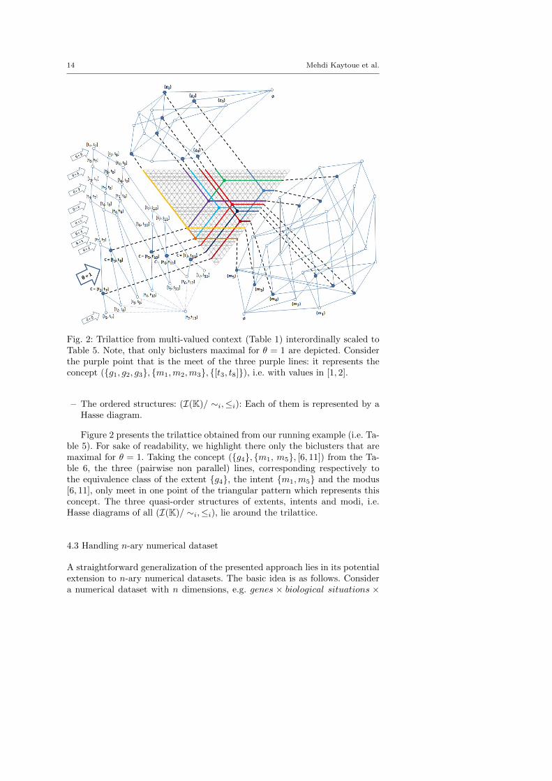
Fig. 2: Trilattice from multi-valued context (Table 1) interordinally scaled toTable 5. Note, that only biclusters maximal for θ = 1 are depicted. Considerthe purple point that is the meet of the three purple lines: it represents theconcept ({g1, g2, g3}, {m1,m2,m3}, {[t3, t8]}), i.e. with values in [1, 2].

– The ordered structures: (I(K)/ ∼i,≤i): Each of them is represented by aHasse diagram.

Figure 2 presents the trilattice obtained from our running example (i.e. Ta-ble 5). For sake of readability, we highlight there only the biclusters that aremaximal for θ = 1. Taking the concept ({g4}, {m1, m5}, [6, 11]) from the Ta-ble 6, the three (pairwise non parallel) lines, corresponding respectively tothe equivalence class of the extent {g4}, the intent {m1,m5} and the modus[6, 11], only meet in one point of the triangular pattern which represents thisconcept. The three quasi-order structures of extents, intents and modi, i.e.Hasse diagrams of all (I(K)/ ∼i,≤i), lie around the trilattice.

4.3 Handling n-ary numerical dataset

A straightforward generalization of the presented approach lies in its potentialextension to n-ary numerical datasets. The basic idea is as follows. Considera numerical dataset with n dimensions, e.g. genes × biological situations ×


timestamps when n = 3. Then, one can extract n-clusters of similar valuesby scaling the numerical data into a n + 1-dimensional binary dataset. So-called polyadic concepts [37] in the binary dataset are here again in 1-to-1-correspondence with maximal n-clusters of similar values of the numericaldataset. We present here theoretical aspects while computing aspects can beregarded with the existing algorithms Data-Peeler [10].

Recall that the standard order on 2k − 1 attributes of the interordinalscale is as follows: [v1, v1], [v1, v2], . . . , [v1, vk], [v2, vk] . . . , [vk, vk]. Having thestandard order on the attributes of the interordinal scale one can enumeratethem from 1 to 2k + 1. Let (G1, . . . , Gn,W, I) be an n-dimensional many-valued context, i.e., an n + 1-dimensional relation I ⊆ G1 × . . . × Gn × Wand W (|W | = q) be the set of numerical values enumerated in the ascendingorder from 1 to q, and let v(g1, . . . , gn) be a map taking the tuple g1, . . . , gnto the value w ∈W . Let the numerical values from W be interordinally scaledwith the standard order on the scale attributes, so we can denote the scaleattributes by m1, . . . ,mq, . . . ,m2q−1. Let B = {m1, . . . ,mq, . . .m2q−1} andY ⊆ G1× . . .×Gn×B be an n+1-ary relation such that (g1, . . . , gn,m) ∈ Y iffthe value w of the n-tuple g1, . . . , gn lies in the interval given by the interordinalattribute m.

Proposition 2 (A1, . . . , An) is a maximal n-way cluster of similar values(Ai ⊆ Gi) with the values lying in the interval [t, t + θ] for t ∈ N, θ ≥ 0iff (A1, . . . , An, U) is an n + 1-adic concept of the n + 1-dimensional context(G1, . . . , Gn, U, Y ), where U = {t + θ, . . . q, . . . , q + t − 1}. Moreover, everyn+ 1-dimensional concept of the interordinally scaled n+ 1-dimensional con-text (G1, . . . , Gn,W, Y ) is of the form (A1, . . . , An, U), where Ai ⊆ Gi, andU = {t+ θ, . . . q, . . . , q + t− 1} for some t ∈ N and θ ≥ 0.

The proof is similar as in the triadic case and hence is omitted.

4.4 Remarks

We showed that extracting biclusters of similar values for any θ in a numericaldataset can be achieved by (i) scaling the attribute value dimension and (ii)extracting the triadic concepts in the resulting derived triadic context. Thesame applies when considering n-ary numerical datasets.

On the one hand, triadic concepts (A,B,U) with the largest sets A,B orC represent large biclusters of similar values. Indeed, the larger |A| and |B|the larger the data covering of the corresponding bicluster. Furthermore, thelarger |U |, the more similar values for bicluster (A,B). Indeed, by the proper-ties of interordinal scaling, the more intervals in U , the smaller their intervalintersection. Mining so-called top-k frequent triadic concepts can accordinglybe achieved with the existing algorithm Data-Peeler [10].

On the other hand, extracting maximal biclusters for all θ may be neitherefficient nor effective with large numerical data: their number tends to be verylarge and not all biclusters are relevant for a given analysis. Furthermore, both


size and density of contexts derived with interordinal scaling are known to beproblematic w.r.t algorithmic scalability, see e.g. [20]. In existing methods ofthe literature, θ is set a priori. We show now how to handle this case withslight modifications, this is our second main result.

5 Extracting biclusters of similar values for a given θ

In this section, we present our second contribution. We consider the problemof extracting maximal biclusters of similar values in TCA for a given θ only.It comes with slight modifications of the methodology presented in the previ-ous section, but requires more algorithmic considerations: although all triadicconcepts correspond to biclusters of similar values with a new transformationprocedure, it is not sure that such concepts correspond to maximal biclusters.In this way, it is not possible to use concepts extraction algorithms directly (orit would require post-processing which is always a solution to avoid). Accord-ingly, a modified scaling procedure will lead us to the design of the algorithmTriMax for a complete and correct extraction of maximal biclusters for agiven θ. Finally, we experiment with this new algorithm.

5.1 Scaling numerical data in a triadic context

Consider the previous scaling applied to a numerical dataset (G,M,W, I). Itscales W into a dimension T and all subsets of T characterize all intervalsof values over W . To get maximal biclusters for a given θ only, we shouldnot consider all possible intervals in W , but rather all intervals (i) having arange size that is less or equal than θ to avoid biclusters with non similarvalues, and (ii) having a range size the closest as possible to θ to avoid non-maximal biclusters. For example, if we set θ = 2, it is probably not interestingto consider interval [0, 8] in the scale dimension since 8 − 0 > θ. Similarly,considering the interval [6, 6] may not be interesting as well, since a biclusterwith all its values equal to 6 may not be maximal. As introduced in [17],the maximal intervals of similar values used for the scale are called blocks oftolerance over the set of numbers W with respect to the tolerance relation'θ. We now recall basics on tolerance relations over a set of numbers. Thisallows us to define a simpler scaling procedure. The resulting triadic contextis then mined with a new TCA algorithm called TriMax to extract maximalbiclusters of similar values for a given θ.

Blocks of tolerance over W are as maximal sets of pairwise similar values:

Definition 17 (Tolerance relation and blocks) A binary relation ' is atolerance if it is reflexive, symmetric but not necessarily transitive. Given aset W , a subset V ⊆ W , and a tolerance relation ' over W , V is a block oftolerance if:(i) ∀w1, w2 ∈ V, w1 ' w2 (pairwise similarity)(ii) ∀w1 6∈ V,∃w2 ∈ V, w1 6' w2 (maximality).


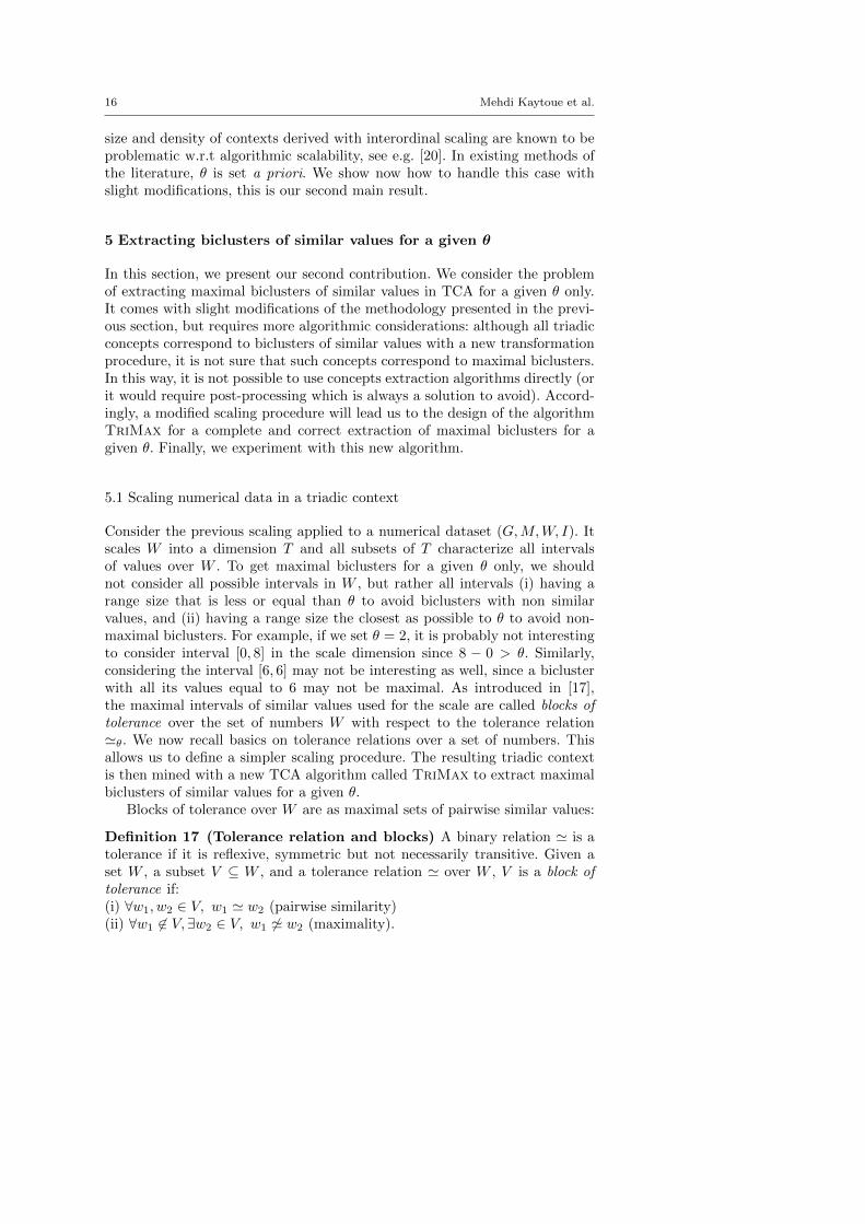
[0, 1] [1, 2] [6, 7] [7, 8] [8, 9]m1 m2 m3 m4 m1 m2 m3 m4 m4 m5 m1 m4 m5 m1 m2

g1 × × × × × × ×g2 × × × × × × ×g3 × × × × × × ×g4 × × × × × × ×

Table 7: Triadic scaled context using tolerance blocks over W and θ = 1 (emptycolumns are not displayed). In gray, the bicluster ({g1, g2, g3}, {m1,m2,m3})with values in [1, 2] and maximal for θ = 1 corresponds to a dyadic concept inthe dyadic context labeled [1, 2].

It follows that 'θ is a tolerance relation. From Table 1 we have W ={0, 1, 2, 6, 7, 8, 9}. With θ = 2, one has 0 '2 2 but 2 6'2 6. Accordingly, oneobtains 3 blocks of tolerance, namely the sets {0, 1, 2}, {6, 7, 8} and {7, 8, 9}.These three sets can be renamed as the convex hull of their elements on N:respectively, [0, 2], [6, 8] and [7, 9]: any number lying between the minimal andthe maximal elements (w.r.t. natural number ordering) of a block of toleranceis naturally similar to any other element of the block. Then, to derive a triadiccontext from a numerical dataset, we simply use tolerance blocks over W todefine the scale dimension.

Definition 18 (TriMax scale relation) The scale relation is a binary re-lation J ⊆ W × C, where C is the set of blocks of tolerance over W renamedas their convex hulls. Then, (w, c) ∈ J iff w ∈ c.

Example 6 From Table 1 we have: C = {[0, 1], [1, 2], [6, 7], [7, 8], [8, 9]} withθ = 1, and C = {[0, 2], [6, 8], [7, 9]} with θ = 2.

In this way, we can apply the same context derivation as in the previoussection: scaling is still based on intervals, but this time it uses tolerance blocks.

Definition 19 (TriMax triadic scaled context) Let Y ⊆ G×M × C bea ternary relation. Then (g,m, c) ∈ Y iff (m(g), c) ∈ J , or simply m(g) ∈ c,where J is the scale relation. (G,M,C, Y ) is called the TriMax triadic scaledcontext.

Example 7 Table 7 is the TriMax triadic scaled context derived from thenumerical dataset lying in Table 1 with θ = 1.

Definition 20 (Dyadic context associated with a block of tolerance)Consider a block of tolerance c ∈ C. The dyadic context associated with thisblock is given by (G,M,Z) where Z denotes the set of all (g,m) ∈ G ×Msuch that m(g) ∈ c.

Example 8 In Table 7, each dyadic context is labeled by its correspondingblock of tolerance for θ = 1.


Now, note that blocks of tolerance over W are totally ordered: let [v1, v2]and [w1, w2] be two blocks of tolerance, one has [v1, v2] < [w1, w2] iff v1 < w1.Hence, associated dyadic contexts are also totally ordered and we can use anindexing set to label them (as done in the algorithm pseudo-code later).

We now present our next results: the scaled triadic context supports theextraction of maximal biclusters of similar values for a given θ. In this casehowever, existing algorithms of TCA cannot be applied directly. For example,in Table 7, the triadic concept ({g3}, {m4}, {[6, 7], [7, 8]}) corresponds to abicluster of similar values which is not maximal. Hence we present hereafter anew TCA algorithm for this task, called TriMax.

The basic idea of TriMax relies on the following facts. Firstly, since eachdyadic context corresponds to a block of tolerance, we do not need to computeintersections of contexts, such as classically done in TCA. Hence each dyadiccontext is processed separately. Secondly, a dyadic concept of a dyadic contextnecessarily represents a bicluster of similar values, but we cannot be sure it ismaximal (see previous example). Hence, we need to check if a concept is still aconcept in other dyadic contexts, corresponding to other classes of tolerance.This is made precise with the following proposition.

Proposition 3 Let (A,B,U) be a triadic concept from TriMax triadic scaledcontext (G,M,C, Y ), such that U is the outer closure of a singleton {c} ⊆ C.If |U | = 1, (A,B) is a maximal bicluster of similar values. Otherwise, (A,B)is a maximal bicluster of similar values iff there is no ∈ [min(U);max(U)],y < c such that (A,B) 6= Ψ

′

y(Ψy((A,B))), where Ψ′

y(·) and Ψy(·) correspond to

inner derivation operators associated with yth dyadic context.

Proof When |U | = 1, (A,B) is a dyadic concept only in one dyadic context cor-responding to a block of tolerance. By properties of tolerance blocks, (A,B) is amaximal bicluster. If |U | 6= 1, (A,B) is a dyadic concept in |U | dyadic contexts.Since the tolerance block set is totally ordered, it directly implies that modusU is the interval [min(U);max(U)]. Hence, if there is y ∈ [min(U);max(U)]such that (A,B) = Ψ

′

y(Ψy((A,B))), then (A,B) is not a maximal bicluster ofsimilar values.

5.2 The TriMax algorithm

TriMax starts with scaling initial numerical data into several dyadic contexts,each one standing for a block of tolerance over W with given θ. The set of alldyadic contexts forms accordingly a triadic context. Then, each dyadic contextis mined with any FCA algorithm (or closed itemset mining algorithm), andall formal concepts are extracted. For a given concept (A,B), we computeouter derivation Φ

′((A,B)), i.e. to obtain the set of dyadic contexts labels in

which the current dyadic concept holds. If this set is a singleton, this meansthat (A,B) is a concept for the current block of tolerance only, i.e. it is amaximal bicluster of similar values, and it has been, or will never be, generatedtwice. Otherwise, (A,B) is a concept in other contexts, and can be generated


accordingly several times (as much as the number of contexts in which itholds). Then, we only consider (A,B) if we are sure it is the last time it iscomputed. Finally, we need to check if current concept represents a maximalbicluster, i.e. there should not exist a context labeled by an element of themodus where (A,B) is not a dyadic concept.

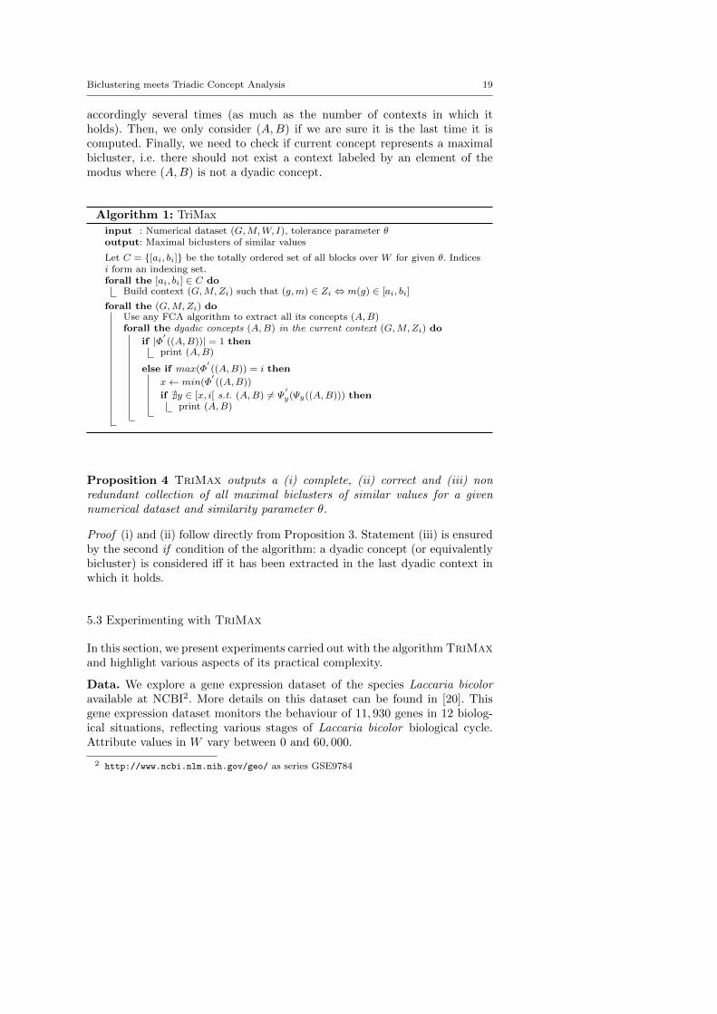
Algorithm 1: TriMax

input : Numerical dataset (G,M,W, I), tolerance parameter θoutput: Maximal biclusters of similar values

Let C = {[ai, bi]} be the totally ordered set of all blocks over W for given θ. Indicesi form an indexing set.forall the [ai, bi] ∈ C do

Build context (G,M,Zi) such that (g,m) ∈ Zi ⇔ m(g) ∈ [ai, bi]

forall the (G,M,Zi) doUse any FCA algorithm to extract all its concepts (A,B)forall the dyadic concepts (A,B) in the current context (G,M,Zi) do

if |Φ′((A,B))| = 1 then

print (A,B)

else if max(Φ′((A,B)) = i then

x← min(Φ′((A,B))

if @y ∈ [x, i[ s.t. (A,B) 6= Ψ′y(Ψy((A,B))) then

print (A,B)

Proposition 4 TriMax outputs a (i) complete, (ii) correct and (iii) nonredundant collection of all maximal biclusters of similar values for a givennumerical dataset and similarity parameter θ.

Proof (i) and (ii) follow directly from Proposition 3. Statement (iii) is ensuredby the second if condition of the algorithm: a dyadic concept (or equivalentlybicluster) is considered iff it has been extracted in the last dyadic context inwhich it holds.

5.3 Experimenting with TriMax

In this section, we present experiments carried out with the algorithm TriMaxand highlight various aspects of its practical complexity.

Data. We explore a gene expression dataset of the species Laccaria bicoloravailable at NCBI2. More details on this dataset can be found in [20]. Thisgene expression dataset monitors the behaviour of 11, 930 genes in 12 biolog-ical situations, reflecting various stages of Laccaria bicolor biological cycle.Attribute values in W vary between 0 and 60, 000.

2 http://www.ncbi.nlm.nih.gov/geo/ as series GSE9784


TriMax implementation. TriMax is written in C++. It uses the boostlibrary 1.42 for data structures and InClose3, an implementation of the al-gorithm CloseByOne [23] for dyadic concept extraction. At each iterationof the main loop, i.e. each tolerance block, the current scaled dyadic contextis produced: We do not generate the whole triadic context which cannot fitinto memory for large databases. It turns out that the modus computationfor a given dyadic concept requires to compute scaling “on the fly”, i.e. whencomputing the set of dyadic contexts in which a current concept holds. Theexperiments were carried out on an Intel CPU 2.54 Ghz machine with 8 GBRAM running under Ubuntu 11.04.

Experiment settings. The goal of the present experiments is not to give aqualitative evaluation of the present approach (say biological interpretation),but rather a quantitative evaluation in terms of computational efficiency. In-deed, the present work aims at showing how an existing type of biclusterscan be mined with Triadic Concept Analysis. For a qualitative evaluation, thereader may refer e.g. to [6,20].

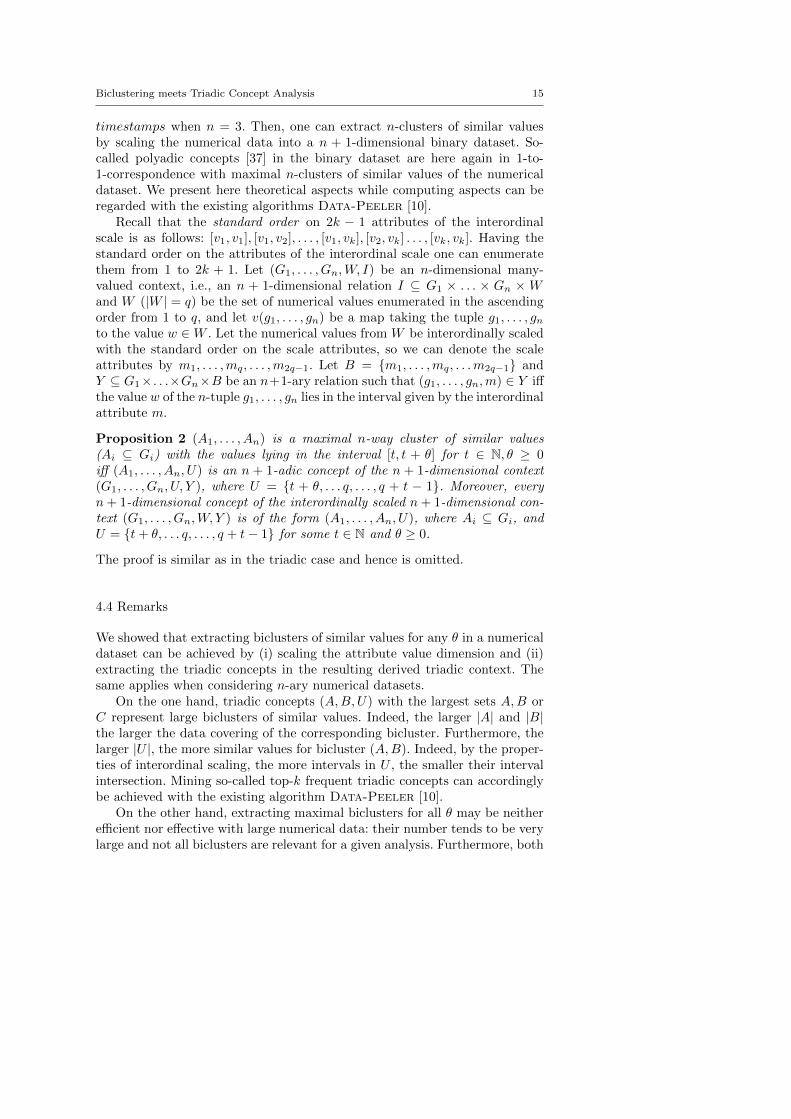
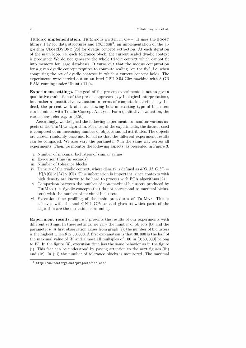
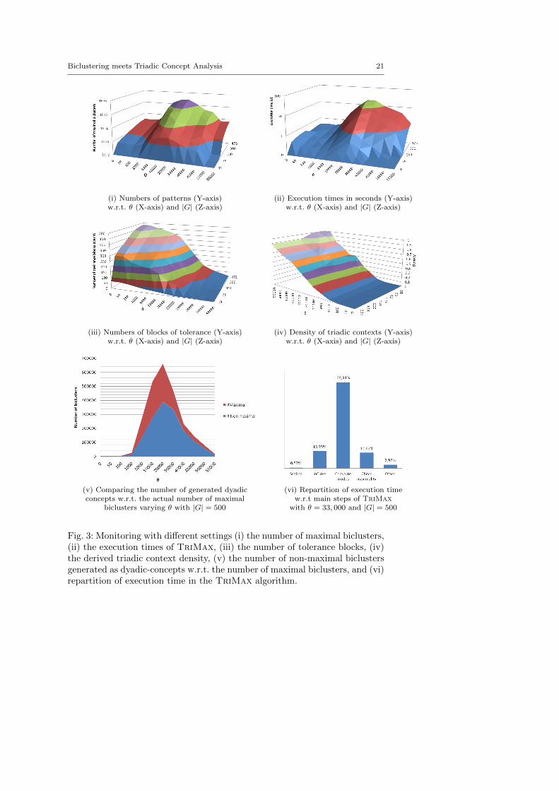
Accordingly, we designed the following experiments to monitor various as-pects of the TriMax algorithm. For most of the experiments, the dataset usedis composed of an increasing number of objects and all attributes. The objectsare chosen randomly once and for all so that the different experiment resultscan be compared. We also vary the parameter θ in the same way across allexperiments. Then, we monitor the following aspects, as presented in Figure 3:

i. Number of maximal biclusters of similar valuesii. Execution time (in seconds)iii. Number of tolerance blocksiv. Density of the triadic context, where density is defined as d(G,M,C, Y ) =|Y |/(|G| × |M | × |C|). This information is important, since contexts withhigh density are known to be hard to process with FCA algorithms [24].

v. Comparison between the number of non-maximal biclusters produced byTriMax (i.e. dyadic concepts that do not correspond to maximal biclus-ters) with the number of maximal biclusters.

vi. Execution time profiling of the main procedures of TriMax. This isachieved with the tool GNU GProf and gives us which parts of thealgorithm are the most time consuming.

Experiment results. Figure 3 presents the results of our experiments withdifferent settings. In these settings, we vary the number of objects |G| and theparameter θ. A first observation arises from graph (i): the number of biclustersis the highest when θ ' 30, 000. A first explanation is that 30, 000 is the half ofthe maximal value of W and almost all multiples of 100 in [0; 60, 000] belongto W . In the figure (ii), execution time has the same behavior as in the figure(i). This fact can be understood by paying attention to the next figures (iii)and (iv). In (iii) the number of tolerance blocks is monitored. The maximal

3 http://sourceforge.net/projects/inclose/


(i) Numbers of patterns (Y-axis) (ii) Execution times in seconds (Y-axis)w.r.t. θ (X-axis) and |G| (Z-axis) w.r.t. θ (X-axis) and |G| (Z-axis)

(iii) Numbers of blocks of tolerance (Y-axis) (iv) Density of triadic contexts (Y-axis)w.r.t. θ (X-axis) and |G| (Z-axis) w.r.t. θ (X-axis) and |G| (Z-axis)

(v) Comparing the number of generated dyadic (vi) Repartition of execution timeconcepts w.r.t. the actual number of maximal w.r.t main steps of TriMax

biclusters varying θ with |G| = 500 with θ = 33, 000 and |G| = 500

Fig. 3: Monitoring with different settings (i) the number of maximal biclusters,(ii) the execution times of TriMax, (iii) the number of tolerance blocks, (iv)the derived triadic context density, (v) the number of non-maximal biclustersgenerated as dyadic-concepts w.r.t. the number of maximal biclusters, and (vi)repartition of execution time in the TriMax algorithm.


number is reached when θ = 0, i.e. |C| = |W |. When θ = max(W ), we have|C| = 1. Now we observe in (iv) that the density follows a reverse behavior:When θ = 0, the density tends towards 0%; when θ = max(W ), then densityequals exactly 1%. Combining both graph (iii) and (iv), the worst cases happenwhen both density and tolerance block count are high.

Another observation, which explains also the execution times, arises fromgraph (v). Here the number of maximal biclusters and the number of non-maximal biclusters generated as dyadic concepts are compared. Here again, theworst case is reached when θ ' 30, 000. Looking at figure (vi), we learn thatthis is however not the major problem. The mostly consuming procedure ofTriMax is the computation of the modus of a dyadic concept. The explanationis that we compute modus with “on the fly scaling”.

Therefore, the bottleneck of our algorithm appears to be the modus com-putation. In practical applications however, the analyst is not interested inall biclusters of similar values. Some constraints are generally defined, suchas a minimal (resp. maximal) number of objects (resp. attributes) in a bi-cluster (A,B), or a minimal area |A| × |B|, etc. Interestingly, most of thoseconstraints can be evaluated on a generated dyadic concept. Therefore, beforecomputing the modus of such concept, we can check such properties and dis-card the concept if it does not respect the constraints. Although not reflectedin this paper, we tested how adding minimal (resp. maximal) size constraintson a bicluster affects both the number of biclusters and the execution times.The results are very interesting: for example with θ = 33, 000, |G| = 500, andminimal (resp. maximal) size for |A| set to 10 (resp. 40), TriMax producesonly 5, 332 maximal biclusters in 2.1 seconds compared to 104, 226 maximalbiclusters extracted in 16.130 seconds without any constraint.

Finally, the most interesting aspect of TriMax is the possibility of its dis-tributed execution. Indeed, each iteration, i.e. for each block of tolerance, canbe achieved independently from the others. Furthermore, the core of TriMaxconsisting in extracting dyadic contexts can also be distributed, see e.g. [22].A deeper investigation remains to be done in this case. Note that althoughthe method description involves W as a set of natural numbers, TriMax candirectly handle numerical data with real (floating point) numbers (since W isa finite set).

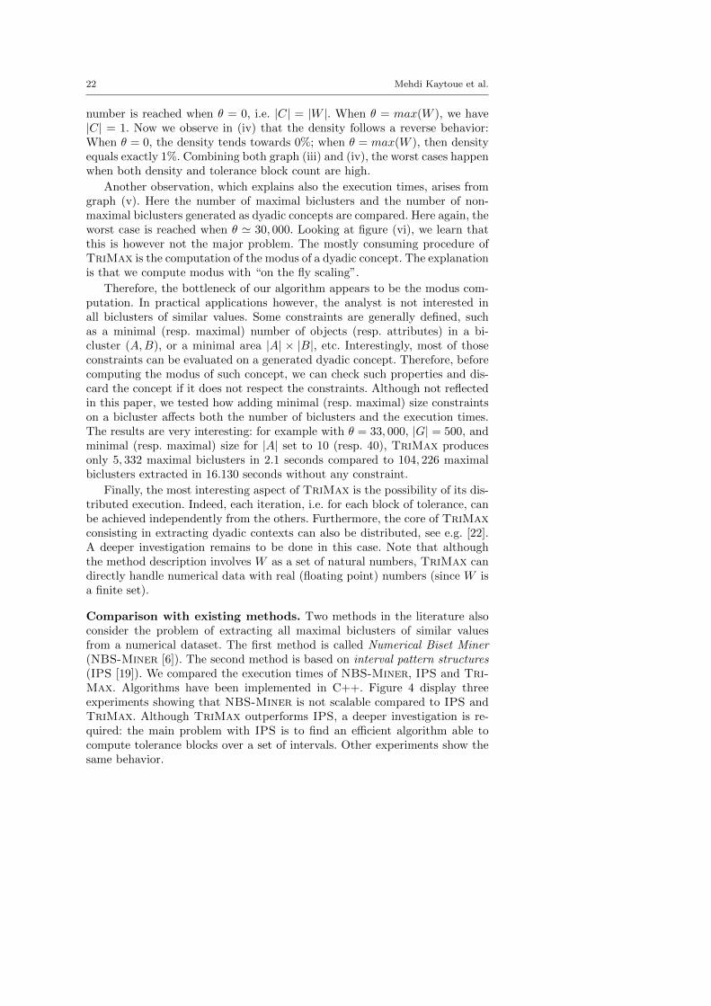
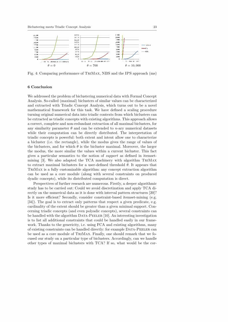
Comparison with existing methods. Two methods in the literature alsoconsider the problem of extracting all maximal biclusters of similar valuesfrom a numerical dataset. The first method is called Numerical Biset Miner(NBS-Miner [6]). The second method is based on interval pattern structures(IPS [19]). We compared the execution times of NBS-Miner, IPS and Tri-Max. Algorithms have been implemented in C++. Figure 4 display threeexperiments showing that NBS-Miner is not scalable compared to IPS andTriMax. Although TriMax outperforms IPS, a deeper investigation is re-quired: the main problem with IPS is to find an efficient algorithm able tocompute tolerance blocks over a set of intervals. Other experiments show thesame behavior.


θ = 0 θ = 700 θ = 10, 000

Fig. 4: Comparing performance of TriMax, NBS and the IPS approach (ms)

6 Conclusion

We addressed the problem of biclustering numerical data with Formal ConceptAnalysis. So-called (maximal) biclusters of similar values can be characterizedand extracted with Triadic Concept Analysis, which turns out to be a novelmathematical framework for this task. We have defined a scaling procedureturning original numerical data into triadic contexts from which biclusters canbe extracted as triadic concepts with existing algorithms. This approach allowsa correct, complete and non-redundant extraction of all maximal biclusters, forany similarity parameter θ and can be extended to n-ary numerical datasetswhile their computation can be directly distributed. The interpretation oftriadic concepts is powerful: both extent and intent allow one to characterizea bicluster (i.e. the rectangle), while the modus gives the range of values ofthe biclusters, and for which θ is the bicluster maximal. Moreover, the largerthe modus, the more similar the values within a current bicluster. This factgives a particular semantics to the notion of support as defined in itemset-mining [3]. We also adapted the TCA machinery with algorithm TriMaxto extract maximal biclusters for a user-defined threshold θ. It appears thatTriMax is a fully customizable algorithm: any concept extraction algorithmcan be used as a core module (along with several constraints on produceddyadic concepts), while its distributed computation is direct.

Perspectives of further research are numerous. Firstly, a deeper algorithmicstudy has to be carried out: Could we avoid discretization and apply TCA di-rectly on the numerical data as it is done with interval pattern structures [20]?Is it more efficient? Secondly, consider constraint-based itemset-mining (e.g.[34]). The goal is to extract only patterns that respect a given predicate, e.g.cardinality of the extent should be greater than a given minimal support. Con-cerning triadic concepts (and even polyadic concepts), several constraints canbe handled with the algorithm Data-Peeler [10]. An interesting investigationis to list all additional constraints that could be handled easily in our frame-work. Thanks to the genericity, i.e. using FCA and existing algorithms, manyof existing constraints can be handled directly: for example Data-Peeler canbe used as a core module of TriMax. Finally, one should remark that we fo-cused our study on a particular type of biclusters. Accordingly, can we handleother types of maximal biclusters with TCA? If so, what would be the cor-


responding scaling? Can we characterize properties that a bicluster definitionshould follow so that TCA can be applied?

Acknowledgements. Authors would like to thank Dmitry A. Morozov forimplementing the algorithms NBS-Miner and IPS. The first author was par-tially supported by CNPq, Fapemig and the Brazilian National Institute forScience and Technology for the Web (InWeb). The second author was sup-ported by the Basic Research Program of the National Research UniversityHigher School of Economics, project “Mathematical models, algorithms, andsoftware for knowledge discovery in structured and text data”. The third au-thor acknowledges support by Grant No. P103/10/1056 of the Czech ScienceFoundation.

References

1. G. Adomavicius and A. Tuzhilin. Toward the next generation of recommender systems: asurvey of the state-of-the-art and possible extensions. Knowledge and Data Engineering,IEEE Transactions on, 17(6):734 – 749, june 2005.

2. R. Agrawal, J. Gehrke, D. Gunopulos, and P. Raghavan. Automatic subspace clusteringof high dimensional data. Data Min. Knowl. Discov., 11(1):5–33, 2005.

3. R. Agrawal, T. Imielinski, and A. N. Swami. Mining association rules between sets ofitems in large databases. In P. Buneman and S. Jajodia, editors, Proceedings of the1993 ACM SIGMOD International Conference on Management of Data, pages 207–216. ACM Press, 1993.

4. F. Alqadah and R. Bhatnagar. Similarity measures in formal concept analysis. Ann.Math. Artif. Intell., 61(3):245–256, 2011.

5. J. Besson, C. Robardet, and J.-F. Boulicaut. Mining a new fault-tolerant pattern typeas an alternative to formal concept discovery. In H. Scharfe, P. Hitzler, and P. hrstrøm,editors, Conceptual Structures: Inspiration and Application, 14th International Con-ference on Conceptual Structures (ICCS), volume 4068 of Lecture Notes in ComputerScience, pages 144–157. Springer, 2006.

6. J. Besson, C. Robardet, L. D. Raedt, and J.-F. Boulicaut. Mining bi-sets in numericaldata. In S. Dzeroski and J. Struyf, editors, KDID, volume 4747 of Lecture Notes inComputer Science, pages 11–23. Springer, 2007.

7. S. Blachon, R. Pensa, J. Besson, C. Robardet, J.-F. Boulicaut, and O. Gandrillon.Clustering Formal Concepts to Discover Biologically Relevant Knowledge from GeneExpression Data. In Silico Biology, 7(4–5):467–483, 2007.

8. R. Braga Araujo, G. Trielli Ferreira, G. Orair, J. Meira, Wagner, R. Celso Ferreira,D. Olavo Guedes Neto, and M. Zaki. The partricluster algorithm for gene expressionanalysis. International Journal of Parallel Programming, 36:226–249, 2008.

9. A. Califano, G. Stolovitzky, and Y. Tu. Analysis of gene expression microarrays forphenotype classification. In Proceedings of the Eighth International Conference onIntelligent Systems for Molecular Biology (ISMB), pages 75–85. AAAI, 2000.

10. L. Cerf, J. Besson, C. Robardet, and J.-F. Boulicaut. Closed patterns meet n-aryrelations. TKDD, 3(1), 2009.

11. Y. Cheng and G. Church. Biclustering of expression data. In Proc. 8th InternationalConference on Intelligent Systems for Molecular Biology (ISBM), pages 93–103, 2000.

12. B. Ganter and R. Wille. Formal Concept Analysis. Springer, 1999.13. J. A. Hartigan. Direct Clustering of a Data Matrix. Journal of the American Statistical

Association, 67(337):123–129, 1972.14. D. I. Ignatov, S. O. Kuznetsov, and J. Poelmans. Concept-based biclustering for internet

advertisement. In J. Vreeken, C. Ling, M. J. Zaki, A. Siebes, J. X. Yu, B. Goethals,G. I. Webb, and X. Wu, editors, ICDM Workshops, pages 123–130. IEEE ComputerSociety, 2012.


15. R. Jaschke, A. Hotho, C. Schmitz, B. Ganter, and G. Stumme. Trias - an algorithm formining iceberg tri-lattices. In ICDM, pages 907–911, 2006.

16. L. Ji, K.-L. Tan, and A. K. H. Tung. Mining frequent closed cubes in 3d datasets. InProceedings of the 32nd International Conference on Very Large Data Bases (VLDB),pages 811–822. ACM, 2006.

17. M. Kaytoue, Z. Assaghir, A. Napoli, and S. O. Kuznetsov. Embedding tolerance rela-tions in formal concept analysis: an application in information fusion. In CIKM, pages1689–1692. ACM, 2010.

18. M. Kaytoue, S. O. Kuznetsov, J. Macko, W. Meira, and A. Napoli. Mining Biclusters ofSimilar Values with Triadic Concept Analysis. In A. Napoli and V. Vychodil, editors,The Eighth International Conference on Concept Lattices and their Applications - CLA2011, Nancy, France, 2011. INRIA Nancy Grand Est - LORIA.

19. M. Kaytoue, S. O. Kuznetsov, and A. Napoli. Biclustering numerical data in formalconcept analysis. In P. Valtchev and R. Jaschke, editors, ICFCA, volume 6628 of LNCS,pages 135–150. Springer, 2011.

20. M. Kaytoue, S. O. Kuznetsov, A. Napoli, and S. Duplessis. Mining gene expression datawith pattern structures in formal concept analysis. Inf. Sci., 181(10):1989–2001, 2011.

21. M. Kaytoue-Uberall, S. Duplessis, S. O. Kuznetsov, and A. Napoli. Two fca-based meth-ods for mining gene expression data. In S. Ferre and S. Rudolph, editors, Proceedings ofthe 7th International Conference on Formal Concept Analysis (ICFCA), volume 5548of Lecture Notes in Computer Science, pages 251–266. Springer, 2009.

22. P. Krajca and V. Vychodil. Distributed algorithm for computing formal concepts usingmap-reduce framework. In IDA, pages 333–344. Springer, 2009.

23. S. O. Kuznetsov. A fast algorithm for computing all intersections of objects in a finitesemi-lattice. Automatic Documentation and Mathematical Linguistics, 27(5):11–21,1993.

24. S. O. Kuznetsov and S. A. Obiedkov. Comparing performance of algorithms for gener-ating concept lattices. J. Exp. Theor. Artif. Intell., 14(2-3):189–216, 2002.

25. F. Lehmann and R. Wille. A triadic approach to formal concept analysis. In ICCS,volume 954 of LNCS, pages 32–43. Springer, 1995.

26. S. Madeira and A. Oliveira. Biclustering algorithms for biological data analysis: a survey.IEEE/ACM Transactions on Computational Biology and Bioinformatics, 1(1):24–45,2004.

27. B. Mirkin. Mathematical classification and clustering. Boston-Dordrecht: Kluwer aca-demic publisher, 1996.

28. B. Mirkin. Clustering for data mining: a data recovery approach. Chapman & Hall/CrcComputer Science, 2005.

29. B. Mirkin and A. V. Kramarenko. Approximate bicluster and tricluster boxes in theanalysis of binary data. In S. O. Kuznetsov, D. Slezak, D. H. Hepting, and B. Mirkin,editors, Proceedings of the 13th International Conference on Rough Sets, Fuzzy Sets,Data Mining and Granular Computing (RSFDGrC 2011), volume 6743 of Lecture Notesin Computer Science, pages 248–256. Springer, 2011.

30. S. Motameny, B. Versmold, and R. Schmutzler. Formal concept analysis for the identifi-cation of combinatorial biomarkers in breast cancer. In R. Medina and S. A. Obiedkov,editors, Formal Concept Analysis, 6th International Conference (ICFCA), volume 4933of Lecture Notes in Computer Science, pages 229–240. Springer, 2008.

31. R. G. Pensa, C. Leschi, J. Besson, and J.-F. Boulicaut. Assessment of discretizationtechniques for relevant pattern discovery from gene expression data. In M. J. Zaki,S. Morishita, and I. Rigoutsos, editors, Proceedings of the 4th ACM SIGKDD Workshopon Data Mining in Bioinformatics (BIOKDD 2004), pages 24–30, 2004.

32. A. Prelic, S. Bleuler, P. Zimmermann, A. Wille, P. Buhlmann, W. Gruissem, L. Hennig,L. Thiele, and E. Zitzler. A Systematic Comparison and Evaluation of BiclusteringMethods for Gene Expression Data. Bioinformatics, 22(9):1122–1129, 2006.

33. C. Raıssi, J. Pei, and T. Kister. Computing closed skycubes. PVLDB, 3(1):838–847,2010.

34. A. Soulet, C. Raıssi, M. Plantevit, and B. Cremilleux. Mining dominant patterns inthe sky. In D. J. Cook, J. Pei, W. Wang, O. R. Zaıane, and X. Wu, editors, 11th IEEEInternational Conference on Data Mining (ICDM), pages 655–664. IEEE, 2011.


35. A. B. Tchagang, S. Phan, F. Famili, H. Shearer, P. R. Fobert, Y. Huang, J. Zou,D. Huang, A. Cutler, Z. Liu, and Y. Pan. Mining biological information from 3dshort time-series gene expression data: the optricluster algorithm. BMC Bioinformatics,13:54, 2012.

36. P. Valtchev, R. Missaoui, and R. Godin. Formal Concept Analysis for Knowledge Dis-covery and Data Mining: The New Challenges. In P. W. Eklund, editor, ICFCA, volume2961 of LNCS, pages 352–371. Springer, 2004.

37. G. Voutsadakis. Polyadic concept analysis. Order, 19(3):295–304, 2002.38. R. Wille. Restructuring lattice theory: an approach based on hierarchies of concepts.

In I. Rival, editor, Ordered Sets, pages 445–470. Reidel, 1982.39. R. Wille. Why Can Concept Lattices Support Knowledge Discovery in Databases? J.

Exp. Theor. Artif. Intell., 14(2-3):81–92, 2002.40. L. Zhao and M. J. Zaki. Tricluster: an effective algorithm for mining coherent clusters in

3d microarray data. In Proceedings of the 2005 ACM SIGMOD international conferenceon Management of data, SIGMOD ’05, pages 694–705, New York, NY, USA, 2005. ACM.

Documents

Biclustering meets Triadic Concept AnalysisBiclustering meets Triadic Concept Analysis Mehdi Kaytoue Sergei O. Kuznetsov Juraj Macko Amedeo Napoli Received: date / Accepted: date Abstract