Embed Size (px)
Citation preview
Strong uniqueness for stochastic evolution equationsin Hilbert spaces perturbed by a bounded
measurable drift
G. Da Prato ∗
Scuola Normale Superiore
Piazza dei Cavalieri 7, 56126 Pisa, Italy
F. Flandoli †
Dipartimento di Matematica Applicata “U. Dini”
Universita di Pisa, Italy
E. Priola ‡
Dipartimento di Matematica, Universita di Torino
via Carlo Alberto 10, Torino, Italy
M. Rockner §
University of Bielefeld, Germany
June 12, 2012
Abstract
We prove pathwise (hence strong) uniqueness of solutions to stochastic evo-lution equations in Hilbert spaces with merely measurable bounded drift andcylindrical Wiener noise, thus generalizing Veretennikov’s fundamental result on
∗E-mail: [email protected]†E-mail: [email protected]‡Partially supported by the M.I.U.R. research project Prin 2008 “Deterministic and stochastic
methods in the study of evolution problems”. E-mail: [email protected]§Research supported by the DFG through IRTG 1132 and CRC 701 and the I. Newton Institute,
Cambridge, UK. E-mail: [email protected]
1
Rd to infinite dimensions. Because Sobolev regularity results implying continu-ity or smoothness of functions, do not hold on infinite dimensional spaces, weemploy methods and results developed in the study of Malliavin-Sobolev spacesin infinite dimensions. The price we pay is that we can prove uniqueness for alarge class, but not for every initial distribution. Such restriction, however, iscommon in infinite dimensions.
Mathematics Subject Classification (2000): 35R60, 60H15
Key words: Pathwise uniqueness, stochastic PDEs, bounded measurable drift.
1 Introduction
We consider the following abstract stochastic differential equation in a separableHilbert space H
dXt = (AXt +B(Xt))dt+ dWt, X0 = x ∈ H (1)
where A : D(A) ⊂ H → H is self–adjoint, negative definite and such that(−A)−1+δ, for some δ ∈ (0, 1), is of trace class, B : H → H and W = (Wt) is acylindrical Wiener process. About B, we only assume that it is Borel measurableand bounded :
B ∈ Bb(H,H)
Our aim is to prove pathwise uniqueness for (1), thus gaining an infinite dimen-sional generalization of the famous fundamental result of Veretennikov [Ve80] inthe case H = Rd. We refer to [Zv74] and [TTW74] for the case H = R as wellas to the generalizations of [Ve80] to unbounded drifts in [KR05], [Zha05] andalso to the references therein. We note that [TTW74] also includes the case ofα-stable noise, α ≥ 1, which in turn was extended to Rd in [Pr10].
Explicit cases of parabolic stochastic partial differential equations, with space-time white noise in space-dimension one, have been solved on various levels ofgenerality for the drift by Gyongy and coworkers, in a series of papers, see [AG01],[Go98], [GN01], [GN99], [GP93] and the references therein. The difference of thepresent paper with respect to these works is that we obtain a general abstractresult, applicable for instance to systems of parabolic equations or equations withdifferential operators of higher order than two. As we shall see, the price to payfor this generality is a restriction on the initial conditions. Indeed, using that forB = 0 there exists a unique non-degenerate (Gaussian) invariant measure µ, wewill prove strong uniqueness for µ-a.e. initial x ∈ H or random H-valued x withdistribution absolutely continuous with respect to µ.
2
At the abstract level, this work generalizes [DF10] devoted to the case whereB is bounded and in addition Holder continuous, but with no restriction on theinitial conditions. To prove our result we use some ideas from [KR05], [FGP10],[DF10] and [FF10].
The extension of Veretennikov’s result [Ve80] and also of [KR05] to infinitedimensions has resisted various attempts of its realization for many years. Thereason is that the finite dimensional results heavily depend on advanced parabolicSobolev regularity results for solutions to the corresponding Kolmogorov equa-tions. Such regularity results, leading to continuity or smoothness of the solu-tions, however, do not hold in infinite dimensions. A technique different from[Ve80] is used in [FGP10] (see also [DF10], [FF10] and [Pr10]). This techniqueallows to prove uniqueness for stochastic equations with time independent coef-ficients by merely using elliptic (not parabolic) regularity results. In the presentpaper we succeed in extending this approach to infinite dimensions, exploitingadvanced regularity results for elliptic equations in Malliavin-Sobolev spaces withrespect to a Gaussian measure on Hilbert space. To the best of our knowledgethis is the first time that an analogue of Veretennikov’s result has been obtained.
Given a filtered probability space (Ω,F , (Ft),P), a cylindrical Wiener processW and an F0-measurable r.v. x, we call mild solution to the Cauchy problem(1) a continuous Ft-adapted H-valued process X = (Xt) such that
Xt = etAx+
∫ t
0e(t−s)AB (Xs) ds+
∫ t
0e(t−s)AdWs. (2)
Existence of mild solutions on some filtered probability space is well known (seeChapter 10 in [DZ92] and also Appendix A.1). Our main result is:
Theorem 1. Assume Hypothesis 1. For µ-a.e. (deterministic) x ∈ H, there isa unique (in the pathwise sense) mild solution of the Cauchy problem (1).
Moreover, for every F0-measurable H-valued r.v. x with law µ0 such thatµ0 << µ and ∫
H
(dµ0dµ
)ζdµ <∞
for some ζ > 1, there is also a unique mild solution of the Cauchy problem.
The proof, performed in Section 3, uses regularity results for elliptic equationsin Hilbert spaces, given in Section 2 where we also establish an Ito type formulainvolving u(Xt) with u in some Sobolev space associated to µ. In comparisonwith the finite dimensional case (cf. [KR05]), to prove such Ito formula we donot only need analytic regularity results, but also the fact that all transitionprobability functions associated to (2) are absolutely continuous with respect to
3
µ. This result heavily depends on an infinite dimensional version of Girsanov’stheorem. Though, also under our conditions, this is a “folklore result” in thefield, it seems hard to find an accessible reference in the literature. Therefore,we include a complete proof of the version we need in the appendix for theconvenience of the reader.
Concerning the proof of Theorem 1 given in Section 3 we remark that, incomparison to the finite dimensional case (see, in particular, [Fe09] and [FF10]),it is necesary to control infinite series of second derivatives of solutions to Kol-mogorov equations which is much more elaborate
Examples are given in Section 4.
1.1 Assumptions and preliminaries
We are given a real separable Hilbert space H and denote its norm and innerproduct by |·| and 〈·, ·〉 respectively. We follow [DZ92], [DZ02], [Da04] and assume
Hypothesis 1 A : D(A) ⊂ H → H is a negative definite self-adjoint operatorand (−A)−1+δ, for some δ ∈ (0, 1), is of trace class.
Since A−1 is compact, there exists an orthonormal basis (ek) in H and asequence of positive numbers (λk) such that
Aek = −λkek, k ∈ N. (3)
Recall that A generates an analytic semigroup etA on H such that etAek =e−λktek. We will consider a cylindrical Wiener process Wt with respect to theprevious basis (ek). The process Wt is formally given by “Wt =
∑k≥1 βk(t)ek”
where βk(t) are independent one dimensional Wiener process (see [DZ92] formore details).
By Rt we denote the Ornstein-Uhlenbeck semigroup in Bb(H) (the Banachspace of Borel and bounded real functions endowed with the essential supremumnorm ‖ · ‖0) defined as
Rtϕ(x) =
∫Hϕ(y)N(etAx,Qt)(dy), ϕ ∈ Bb(H), (4)
where N(etAx,Qt) is the Gaussian measure in H of mean etAx and covarianceoperator Qt given by,
Qt = −1
2A−1(I − e2tA), t ≥ 0. (5)
We notice that Rt has a unique invariant measure µ := N(0, Q) where Q =−1
2 A−1. Moreover, since under the previous assumptions, the Ornstein-Uhlenbeck
4
semigroup is strong Feller and irreducible we have by Doob’s theorem that, forany t > 0, x ∈ H, the measures N(etAx,Qt) and µ are equivalent (see [DZ02]).On the other hand, our assumption that (−A)−1+δ is trace class guarantees thatthe OU process
Zt = Z(t, x) = etAx+
∫ t
0e(t−s)AdWs (6)
has a continuous H-valued version.If H and K are separable Hilbert spaces, the Banach space Lp(H,µ, K), p ≥
1, is defined to consist of equivalent classes of measurable functions f : H → Ksuch that
∫H |f |
pK µ(dx) < +∞ (if K = R we set Lp(H,µ,R) = Lp(H,µ)). We
also use the notation Lp(µ) instead of Lp(H,µ,K) when no confusion may arise.The semigroup Rt can be uniquely extended to a strongly continuous semi-
group of contractions on Lp(H,µ), p ≥ 1, which we still denote by Rt, whereaswe denote by Lp (or L when no confusion may arise) its infinitesimal generator,which is defined on smooth functions ϕ as
Lϕ(x) =1
2Tr(D2ϕ(x)) + 〈Ax,Dϕ(x)〉,
where Dϕ(x) and D2ϕ(x) denote respectively the first and second Frechet deriva-tives of ϕ at x ∈ H. For Banach spaces E and F we denote by Ckb (E,F ), k ≥ 1,the Banach space of all functions f : E → F which are bounded and Frechetdifferentiable on E up to the order k ≥ 1 with all derivatives bounded andcontinuous. We also set Ckb (E,R) = Ckb (E).
According to [DZ02], for any ϕ ∈ Bb(H) and any t > 0 one has Rtϕ ∈C∞b (H) = ∩k≥1Ckb (H). Moreover,
〈DRtϕ(x), h〉 =
∫H〈Λth,Q
− 12
t y〉ϕ(etAx+ y)N(0, Qt)(dy), h ∈ H, (7)
where Qt is defined in (5),
Λt = Q−1/2t etA =
√2 (−A)1/2etA(I − e2tA)−1/2 (8)
and y 7→ 〈Λth,Q− 1
2t y〉 is a centered Gaussian random variable under µt =
N(0, Qt) with variance |Λth|2 for any t > 0 (cf. [DZ92, Theorem 6.2.2]). Since
Λtek =√
2 (λk)1/2e−tλk(1− e−2tλk)−1/2ek,
we see that, for any ε ∈ [0,∞), there exists Cε > 0 such that
‖(−A)εΛt‖L ≤ Cεt−12−ε. (9)
5
In the sequel ‖ · ‖ always denotes the Hilbert-Schmidt norm; on the other hand‖ · ‖L indicates the operator norm.
By (7) we deduce
supx∈H|(−A)εDRtϕ(x)| = ‖(−A)εDRtϕ‖0 ≤ Cεt−
12−ε‖ϕ‖0, (10)
which by taking the Laplace transform yields, for ε ∈ [0, 1/2),
‖(−A)εD (λ− L2)−1ϕ‖0 ≤
C1,ε
λ12−ε‖ϕ‖0. (11)
Similarly, we find
‖(−A)εDRtϕ‖L2(µ) ≤ Cεt−12−ε ‖ϕ‖L2(µ) (12)
and
‖(−A)εD (λ− L2)−1ϕ‖L2(µ) ≤
C1,ε
λ12−ε‖ϕ‖L2(µ). (13)
Recall that the Sobolev space W 2,p(H,µ), p ≥ 1, is defined in [CG02, Section 3]as the completion of a suitable set of smooth functions endowed with the Sobolevnorm (see also [DZ92, Section 9.2] for the case p = 2 and [Sc92]). Under ourinitial assumptions, the following result can be found in [DZ02, Section 10.2.1].
Theorem 2. Let λ > 0, f ∈ L2(H,µ) and let ϕ ∈ D(L2) be the solution of theequation
λϕ− L2ϕ = f. (14)
Then ϕ ∈ W 2,2(H,µ), (−A)1/2Dϕ ∈ L2(H,µ) and there exists a constant C(λ)such that
‖ϕ‖L2(µ) +(∫
H‖D2ϕ(x)‖2 µ(dx)
)1/2+ ‖(−A)1/2Dϕ‖L2(µ) ≤ C‖f‖L2(µ) (15)
The following extension to Lp(µ), p > 1, can be found in Section 3 of [CG02](see also [CG01] and [MV11]; a finite dimensional result analogous to this fornon-symmetric OU operators was proved in [MPRS02]).
Theorem 3. Let λ > 0, f ∈ Lp(H,µ) and let ϕ ∈ D(Lp) be the solution of theequation
λϕ− Lp ϕ = f. (16)
Then ϕ ∈ W 2,p(H,µ), (−A)1/2Dϕ ∈ Lp(H,µ;H) and there exists a constantC = C(λ, p) such that
‖ϕ‖Lp(µ) +(∫
H‖D2ϕ(x)‖p µ(dx)
)1/p+ ‖(−A)1/2Dϕ‖Lp(µ) ≤ C‖f‖Lp(µ). (17)
6
2 Analytic results and an Ito type formula
2.1 Existence and uniqueness for the Kolmogorov equa-tion
We are here concerned with the equation
λu− L2u− 〈B,Du〉 = f, (18)
where λ > 0, f ∈ Bb(H) and B ∈ Bb(H,H).
Remark 4. Since the corresponding Dirichlet form
E(u, v) :=
∫H〈Du,Dv〉dµ−
∫H〈B,Du〉v dµ+ λ
∫Huv dµ,
u, v ∈ W 1,2(µ), is weakly sectorial for λ big enough, it follows by [MR92, Chap.I and Subsection 3e) in Chap. II] that (18) has a unique solution in D(L2).However we need more regularity for u.
Proposition 5. Let λ ≥ λ0, where
λ0 := 4‖B‖20C21,0. (19)
Then there is a unique solution u ∈ D(L2) of (18) given by
u = uλ = (λ− L2)−1(I − Tλ)−1f, (20)
whereTλϕ := 〈B,D(λ− L2)
−1ϕ〉. (21)
Moreover, u ∈ C1b (H) with
‖u‖0 ≤ 2‖f‖0, ‖(−A)εDu‖0 ≤2C1,ε
λ12−ε‖f‖0, ε ∈ [0, 1/2), (22)
and, for any p ≥ 2, u ∈W 2,p(H,µ) and, for some C = C(λ, p, ‖B‖0),∫H‖D2u(x)‖p µ(dx) ≤ C
∫H|f(x)|p µ(dx). (23)
Proof. Setting ψ := λu− L2u, equation (18) reduces to
ψ − Tλψ = f. (24)
7
If λ ≥ λ0 by (13) we have
‖Tλϕ‖L2(µ) ≤1
2‖ϕ‖L2(µ), ϕ ∈ L2(µ),
so that (24) has an unique solution given by
ψ = (I − Tλ)−1f.
Consequently, (18) has a unique solution u ∈ L2(H,µ) given by (20). The sameargument in Bb(H), using (11) instead of (13) shows that
‖Tλϕ‖0 ≤1
2‖ϕ‖0, ϕ ∈ Bb(H),
and that ψ ∈ Bb(H) and hence by (20) also u ∈ Bb(H). In particular, (22) isfulfilled by (11). To prove the last assertion we write λu − L2u = 〈B,Du〉 + fand use estimate (22) with ε = 0 and Theorem 3.
2.2 Approximations
We are given two sequences (fn) ⊂ Bb(H) and (Bn) ⊂ Bb(H,H) such that
(i) fn(x)→ f(x), Bn(x)→ B(x) µ-a.s..
(ii) ‖fn‖0 ≤M, ‖Bn‖0 ≤M.(25)
Proposition 6. Let λ ≥ λ0, where λ0 is defined in (19). Then the equation
λun − Lun − 〈Bn, Dun〉 = fn, (26)
has a unique solution un ∈ C1b (H) ∩D(L2) given by
un = (λ− L)−1(I − Tn,λ)−1fn, (27)
whereTn,λϕ := 〈Bn, D(λ− L2)
−1ϕ〉. (28)
Moreover, for any ε ∈ [0, 1/2), with constants independent of n,
‖un‖0 ≤ 2M, ‖(−A)εDun‖0 ≤2C1,ε
λ12−εM, (29)
Finally, we have un → u, and Dun → Du, in L2(µ), where u is the solution to(18).
8
Proof. Setψn := (I − Tn,λ)−1fn, ψ := (I − Tλ)−1f.
It is enough to show that
ψn → ψ in L2(H,µ). (30)
Let λ ≥ λ0 and write
ψ − ψn = Tλψ − Tn,λψn + f − fn.
Then, setting ‖ · ‖2 = ‖ · ‖L2(µ),
‖ψ − ψn‖2 ≤ ‖Tn,λψ − Tn,λψn‖2 + ‖Tλψ − Tn,λψ‖2 + ‖f − fn‖2
≤ 12 ‖ψ − ψn‖2 + ‖Tλψ − Tn,λψ‖2 + ‖f − fn‖2.
Consequently
‖ψ − ψn‖2 ≤ 2‖Tλψ − Tn,λψ‖2 + 2‖f − fn‖2.
We also have
‖Tλψ − Tn,λψ‖22 ≤∫H|B(x)−Bn(x)|2|D(λ− L2)
−1ψ(x)|2µ(dx).
Therefore, by the dominate convergence theorem it follows that
limn→∞
‖Tλψ − Tn,λψ‖2 = 0.
The conclusion follows.
2.3 Modified mild formulation
For any i ∈ N we denote the ith component of B by B(i), i.e.,
B(i)(x) := 〈B(x), ei〉.
Then for λ ≥ λ0 we consider the solution u(i) of the equation
λu(i) − Lu(i) − 〈B,Du(i)〉 = B(i), µ -a.s. (31)
9
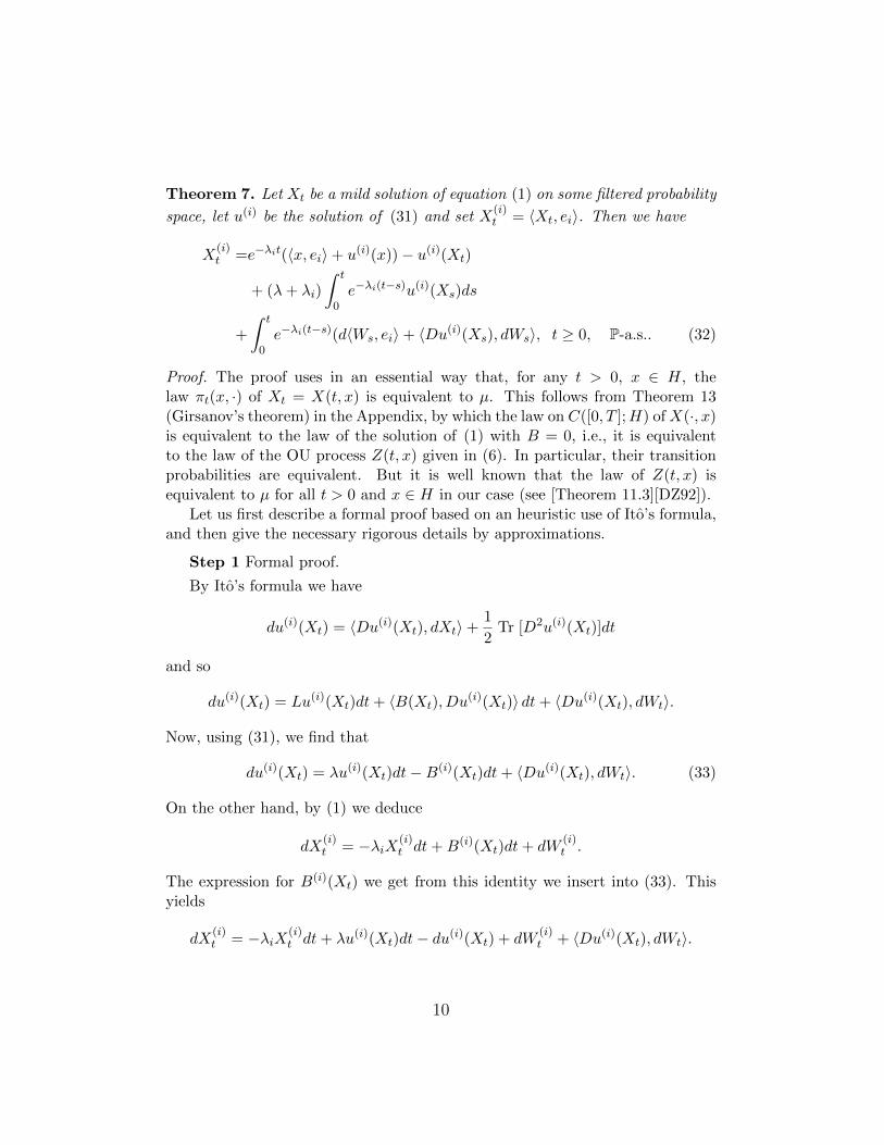
Theorem 7. Let Xt be a mild solution of equation (1) on some filtered probability
space, let u(i) be the solution of (31) and set X(i)t = 〈Xt, ei〉. Then we have
X(i)t =e−λit(〈x, ei〉+ u(i)(x))− u(i)(Xt)
+ (λ+ λi)
∫ t
0e−λi(t−s)u(i)(Xs)ds
+
∫ t
0e−λi(t−s)(d〈Ws, ei〉+ 〈Du(i)(Xs), dWs〉, t ≥ 0, P-a.s.. (32)
Proof. The proof uses in an essential way that, for any t > 0, x ∈ H, thelaw πt(x, ·) of Xt = X(t, x) is equivalent to µ. This follows from Theorem 13(Girsanov’s theorem) in the Appendix, by which the law on C([0, T ];H) ofX(·, x)is equivalent to the law of the solution of (1) with B = 0, i.e., it is equivalentto the law of the OU process Z(t, x) given in (6). In particular, their transitionprobabilities are equivalent. But it is well known that the law of Z(t, x) isequivalent to µ for all t > 0 and x ∈ H in our case (see [Theorem 11.3][DZ92]).
Let us first describe a formal proof based on an heuristic use of Ito’s formula,and then give the necessary rigorous details by approximations.
Step 1 Formal proof.
By Ito’s formula we have
du(i)(Xt) = 〈Du(i)(Xt), dXt〉+1
2Tr [D2u(i)(Xt)]dt
and so
du(i)(Xt) = Lu(i)(Xt)dt+ 〈B(Xt), Du(i)(Xt)〉 dt+ 〈Du(i)(Xt), dWt〉.
Now, using (31), we find that
du(i)(Xt) = λu(i)(Xt)dt−B(i)(Xt)dt+ 〈Du(i)(Xt), dWt〉. (33)
On the other hand, by (1) we deduce
dX(i)t = −λiX(i)
t dt+B(i)(Xt)dt+ dW(i)t .
The expression for B(i)(Xt) we get from this identity we insert into (33). Thisyields
dX(i)t = −λiX(i)
t dt+ λu(i)(Xt)dt− du(i)(Xt) + dW(i)t + 〈Du(i)(Xt), dWt〉.
10
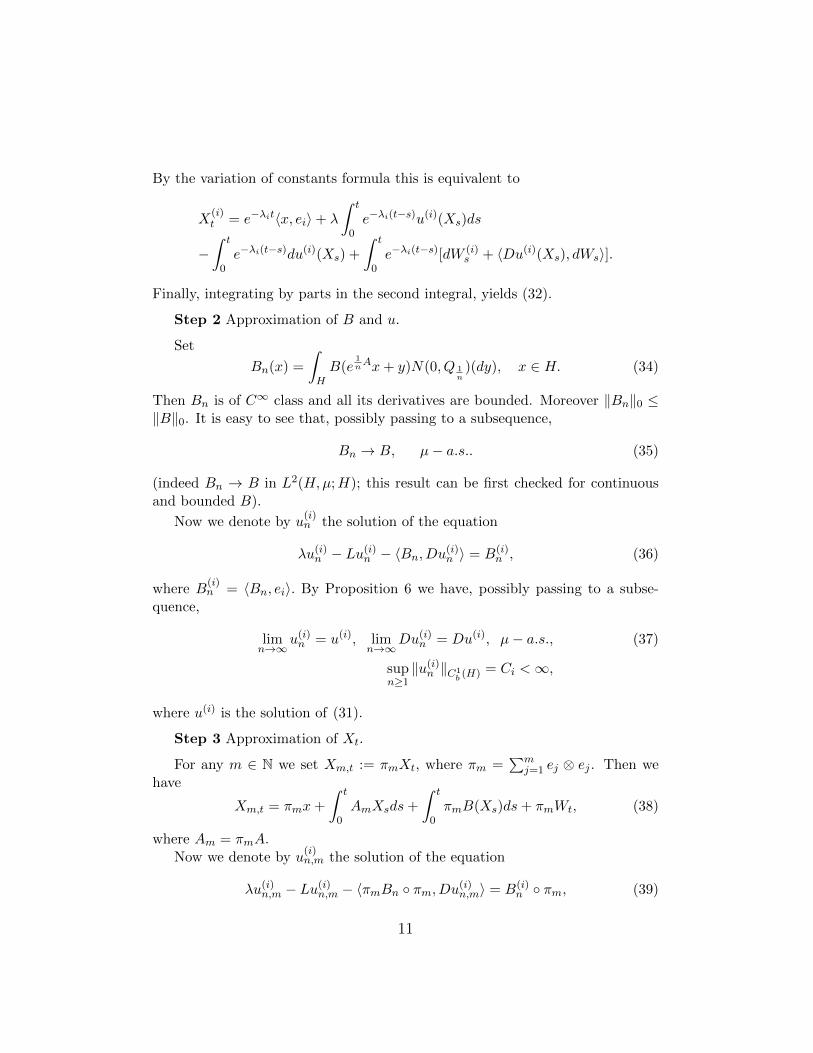
By the variation of constants formula this is equivalent to
X(i)t = e−λit〈x, ei〉+ λ
∫ t
0e−λi(t−s)u(i)(Xs)ds
−∫ t
0e−λi(t−s)du(i)(Xs) +
∫ t
0e−λi(t−s)[dW (i)
s + 〈Du(i)(Xs), dWs〉].
Finally, integrating by parts in the second integral, yields (32).
Step 2 Approximation of B and u.
Set
Bn(x) =
∫HB(e
1nAx+ y)N(0, Q 1
n)(dy), x ∈ H. (34)
Then Bn is of C∞ class and all its derivatives are bounded. Moreover ‖Bn‖0 ≤‖B‖0. It is easy to see that, possibly passing to a subsequence,
Bn → B, µ− a.s.. (35)
(indeed Bn → B in L2(H,µ;H); this result can be first checked for continuousand bounded B).
Now we denote by u(i)n the solution of the equation
λu(i)n − Lu(i)n − 〈Bn, Du(i)n 〉 = B(i)n , (36)
where B(i)n = 〈Bn, ei〉. By Proposition 6 we have, possibly passing to a subse-
quence,
limn→∞
u(i)n = u(i), limn→∞
Du(i)n = Du(i), µ− a.s., (37)
supn≥1‖u(i)n ‖C1
b (H) = Ci <∞,
where u(i) is the solution of (31).
Step 3 Approximation of Xt.
For any m ∈ N we set Xm,t := πmXt, where πm =∑m
j=1 ej ⊗ ej . Then wehave
Xm,t = πmx+
∫ t
0AmXsds+
∫ t
0πmB(Xs)ds+ πmWt, (38)
where Am = πmA.Now we denote by u
(i)n,m the solution of the equation
λu(i)n,m − Lu(i)n,m − 〈πmBn πm, Du(i)n,m〉 = B(i)n πm, (39)
11
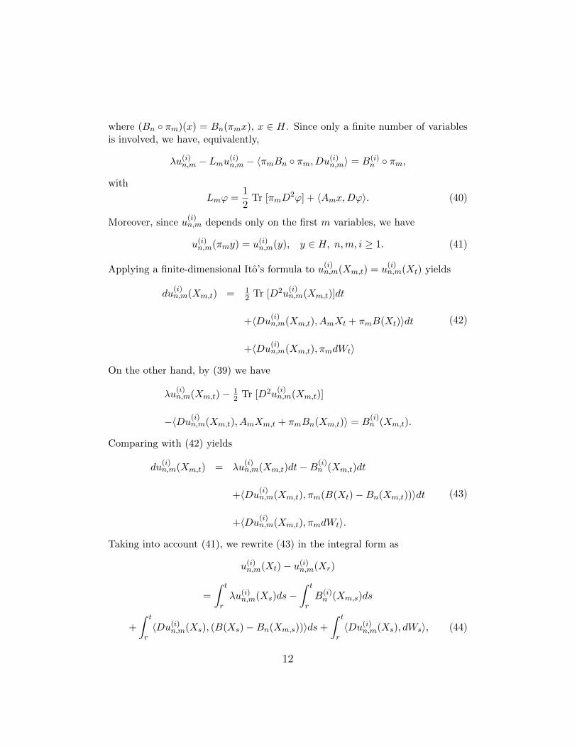
where (Bn πm)(x) = Bn(πmx), x ∈ H. Since only a finite number of variablesis involved, we have, equivalently,
λu(i)n,m − Lmu(i)n,m − 〈πmBn πm, Du(i)n,m〉 = B(i)n πm,
with
Lmϕ =1
2Tr [πmD
2ϕ] + 〈Amx,Dϕ〉. (40)
Moreover, since u(i)n,m depends only on the first m variables, we have
u(i)n,m(πmy) = u(i)n,m(y), y ∈ H, n,m, i ≥ 1. (41)
Applying a finite-dimensional Ito’s formula to u(i)n,m(Xm,t) = u
(i)n,m(Xt) yields
du(i)n,m(Xm,t) = 1
2 Tr [D2u(i)n,m(Xm,t)]dt
+〈Du(i)n,m(Xm,t), AmXt + πmB(Xt)〉dt
+〈Du(i)n,m(Xm,t), πmdWt〉
(42)
On the other hand, by (39) we have
λu(i)n,m(Xm,t)− 1
2 Tr [D2u(i)n,m(Xm,t)]
−〈Du(i)n,m(Xm,t), AmXm,t + πmBn(Xm,t)〉 = B(i)n (Xm,t).
Comparing with (42) yields
du(i)n,m(Xm,t) = λu
(i)n,m(Xm,t)dt−B(i)
n (Xm,t)dt
+〈Du(i)n,m(Xm,t), πm(B(Xt)−Bn(Xm,t))〉dt
+〈Du(i)n,m(Xm,t), πmdWt〉.
(43)
Taking into account (41), we rewrite (43) in the integral form as
u(i)n,m(Xt)− u(i)n,m(Xr)
=
∫ t
rλu(i)n,m(Xs)ds−
∫ t
rB(i)n (Xm,s)ds
+
∫ t
r〈Du(i)n,m(Xs), (B(Xs)−Bn(Xm,s))〉ds+
∫ t
r〈Du(i)n,m(Xs), dWs〉, (44)
12
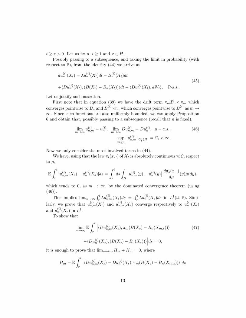
t ≥ r > 0. Let us fix n, i ≥ 1 and x ∈ H.Possibly passing to a subsequence, and taking the limit in probability (with
respect to P), from the identity (44) we arrive at
du(i)n (Xt) = λu
(i)n (Xt)dt−B(i)
n (Xt)dt
+〈Du(i)n (Xt), (B(Xt)−Bn(Xt))〉dt+ 〈Du(i)n (Xt), dWt〉, P-a.s..
(45)
Let us justify such assertion.First note that in equation (39) we have the drift term πmBn πm which
converges pointwise to Bn and B(i)n πm which converges pointwise to B
(i)n as m→
∞. Since such functions are also uniformly bounded, we can apply Proposition6 and obtain that, possibly passing to a subsequence (recall that n is fixed),
limm→∞
u(i)n,m = u(i)n , limm→∞
Du(i)n,m = Du(i)n , µ− a.s., (46)
supm≥1‖u(i)n,m‖C1
b (H) = Ci <∞.
Now we only consider the most involved terms in (44).We have, using that the law πt(x, ·) of Xt is absolutely continuous with respect
to µ,
E∫ t
r|u(i)n,m(Xs)− u(i)n (Xs)|ds =
∫ t
rds
∫H
∣∣u(i)n,m(y)− u(i)n (y)∣∣ dπs(x, ·)
dµ(y)µ(dy),
which tends to 0, as m → ∞, by the dominated convergence theorem (using(46)).
This implies limm→∞∫ tr λu
(i)n,m(Xs)ds =
∫ tr λu
(i)n (Xs)ds in L1(Ω,P). Simi-
larly, we prove that u(i)n,m(Xt) and u
(i)n,m(Xr) converge respectively to u
(i)n (Xt)
and u(i)n (Xr) in L1.
To show that
limm→∞
E∫ t
r
∣∣∣〈Du(i)n,m(Xs), πm(B(Xs)−Bn(Xm,s))〉 (47)
−〈Du(i)n (Xs), (B(Xs)−Bn(Xs))〉∣∣∣ds = 0,
it is enough to prove that limm→∞Hm +Km = 0, where
Hm = E∫ t
r
∣∣〈Du(i)n,m(Xs)−Du(i)n (Xs), πm(B(Xs)−Bn(Xm,s))〉∣∣ds
13
and
Km = E∫ t
r
∣∣〈Du(i)n (Xs), [πmB(Xs)−B(Xs)] + [Bn(Xs)− πmBn(Xm,s)]〉∣∣ds.
It is easy to check that limm→∞Km = 0. Let us deal with Hm. We have
Hm ≤ 2‖B‖0∫ t
rE∣∣Du(i)n,m(Xs)−Du(i)n (Xs)
∣∣ds (48)
≤∫ t
rds
∫H
∣∣Du(i)n,m(y)−Du(i)n (y)∣∣ dπs(x, ·)
dµ(y)µ(dy)
which tends to 0 as m→∞ by the dominated convergence theorem (using (46)).This shows (47).
It remains to prove that
limm→∞
∫ t
r〈Du(i)n,m(Xs), dWs〉 =
∫ t
r〈Du(i)n (Xs), dWs〉, in L2(Ω,P).
To this purpose we use the isometry formula together with
limm→∞
∫ t
rE∣∣∣Du(i)n,m(Xs)−Du(i)n (Xs)
∣∣∣2 ds = 0
(which can be proved arguing as in (48)). Thus we have proved (45).In order to pass to the limit as n → ∞ in (45) we recall formula (37) and
argue as before (using also that πt(x, ·) << µ). We find
u(i)(Xt)− u(i)(Xr) (49)
=
∫ t
rλu(i)(Xs)ds−
∫ t
rB(i)(Xs)ds+
∫ t
r〈Du(i)(Xs), dWs〉,
t ≥ r > 0. Since u is continuous and trajectories of (Xt) are continuous, we canpass to the limit as r → 0+ in (49), P-a.s., and obtain an integral identity on[0, t].
ButdX
(i)t = −λiX(i)
t dt+B(i)(Xt)dt+ dW(i)t , P-a.s..
Now we proceed as in Step 1. Namely, we derive B(i)(Xt) from the identity aboveand insert in (49); this yields
dX(i)t = −λiX(i)
t dt+ λu(i)(Xt)dt− du(i)(Xt) + dW(i)t + 〈Du(i)(Xt), dWt〉,
P-a.s.. Then we use the variation of constants formula.
14
Remark 8. Formula (49) with r = 0 seems to be of independent interest. Asan application, one can deduce, when x ∈ H is deterministic, the representationformula
E[u(i)(Xt)] =
∫ ∞0
e−λtE[B(i)(Xt)]dt.
This follows by taking the Laplace transform in both sides of (49) (with r = 0)and integrating by parts with respect to t.
The next lemma shows that u(x) =∑
k≥1 u(k)(x)ek (u(k) as in (31)) is a well
defined function which belongs to C1b (H,H). Recall that λ0 is defined in (19).
Lemma 9. For λ sufficiently large, i.e., λ ≥ λ, with λ = λ(A, ‖B‖0) there existsa unique u = uλ ∈ C1
b (H,H) which solves
u(x) =
∫ ∞0
e−λtRt(Du(·)B(·) +B(·)
)(x)dt, x ∈ H,
where Rt is the OU semigroup defined as in (4) and acting on H-valued functions.Moreover, we have the following assertions.
(i) Let ε ∈ [0, 1/2[. Then, for any h ∈ H, (−A)εDu(·)[h] ∈ Cb(H,H) and‖(−A)εDu(·)[h]‖0 ≤ Cε,λ|h|;
(ii) for any k ≥ 1, 〈u(·), ek〉 = u(k), where u(k) is the solution defined in (31);(iii) There exists c3 = c3(A, ‖B‖0) > 0 such that, for any λ ≥ λ, u = uλ
satisfies
‖Du‖0 ≤c3√λ. (50)
Proof. Let E = C1b (H,H) and define the operator Sλ,
Sλv(x) =
∫ ∞0
e−λtRt(Dv(·)B(·) +B(·)
)(x)dt, v ∈ E, x ∈ H.
To prove that Sλ : E → E we take into account estimate (11) with ε = 0.Note that to check the Frechet differentiability of Sλv in each x ∈ H we firstshow its Gateaux differentiability. Then using formulas (7) and (11) we obtainthe continuity of the Gateaux derivative from H into L(H) (L(H) denotes theBanach space of all bounded linear operators from H into H endowed with ‖·‖L)and this implies in particular the Frechet differentiability.
For λ ≥ (λ0 ∨ 2‖B‖0), Sλ is a contraction and so there exists a unique u ∈ Ewhich solves u = Sλu. Using again (11) we obtain (i). Moreover, (ii) can bededuced from the fact that, for each k ≥ 1, uk = 〈u(·), ek〉 is the unique solutionto the equation
uk(x) =
∫ ∞0
e−λtRt(〈Duk(·), B(·)〉+Bk(·)
)(x)dt, x ∈ H,
15
in C1b (H) (the uniqueness follows by the contraction principle) and also the func-
tion u(k) ∈ C1b (H) given in (31) solves such equation. Finally (iii) follows easily
from the estimate
‖Du‖0 ≤C1,0
λ1/2(‖Du‖0 ‖B‖0 + ‖B‖0), λ ≥ (λ0 ∨ ‖B‖0).
3 Proof of Theorem 1
We start now the proof of pathwise uniqueness.Let X = (Xt) and Y = (Yt) be two continuous Ft-adapted mild solutions
(defined on the same filtered probability space, solutions with respect to thesame cylindrical Wiener process), starting from the same x.
For the time being, x is not specified (it may be also random, F0-measurable).In the last part of the proof a restriction on x will emerge.
Let us fix T > 0. Let u = uλ : H → H be such that u(x) =∑
i≥1 u(i)(x)ei,
x ∈ H, where u(i) = u(i)λ solve (31) for some λ large enough (see Proposition 5).
By (50) we may assume that ‖Du‖0 ≤ 1/2. We have, for t ∈ [0, T ],
Xt − Yt = u (Yt)− u (Xt) + (λ−A)
∫ t
0e(t−s)A (u (Xs)− u (Ys)) ds
+
∫ t
0e(t−s)A(Du (Xs)−Du(Ys))dWs.
It follows that
|Xt − Yt| ≤1
2|Xt − Yt|+
∣∣∣ (λ−A)
∫ t
0e(t−s)A (u (Xs)− u (Ys)) ds
∣∣∣+∣∣∣ ∫ t
0e(t−s)A(Du (Xs)−Du(Ys))dWs
∣∣∣.Let τ be a stopping time to be specified later. Using that 1[0,τ ](t) = 1[0,τ ](t)·1[0,τ ](s), 0 ≤ s ≤ t ≤ T , we have (cf. [DZ92, page 187])
1[0,τ ](t) |Xt − Yt| ≤ C 1[0,τ ](t)∣∣∣ (λ−A)
∫ t
0e(t−s)A (u (Xs)− u (Ys)) ds
∣∣∣+ C
∣∣∣∣1[0,τ ](t)∫ t
0e(t−s)A (Du (Xs)−Du (Ys)) 1[0,τ ](s) dWs
∣∣∣∣ ,16
where by C we denote any constant which may depend on the assumptions onA, B and T .
Writing 1[0,τ ](s)Xs = Xs and 1[0,τ ](s)Ys = Ys, and, using the Burkholder-Davis-Gundy inequality with a large exponent q > 2 which will be determinedbelow, we obtain (recall that ‖·‖ is the Hilbert-Schmidt norm, cf. [DZ92, Chapter4]) with C = Cq,
E[∣∣∣Xt − Yt
∣∣∣q] ≤ C E[eλqt
∣∣∣∣(λ−A)
∫ t
0e(t−s)Ae−λs(u(Xs)− u(Ys))1[0,τ ](s)ds
∣∣∣∣q]+ CE
[(∫ t
01[0,τ ](s)
∥∥∥e(t−s)A (Du (Xs)−Du (Ys))∥∥∥2 ds)q/2] .
In the sequel we introduce a parameter θ > 0 and Cθ will denote suitable con-stants such that Cθ → 0 as θ → +∞ (the constants may change from line toline). This idea of introducing θ and Cθ is suggested by [Is11, page 8]. Similarly,we will indicate by C(λ) suitable constants such that C(λ)→ 0 as λ→ +∞.
From the previous inequality we deduce, multiplying by e−qθt, for any θ > 0,
E[e−qθt
∣∣∣Xt − Yt∣∣∣q] (51)
≤ CE[∣∣∣∣(λ−A)
∫ t
0e−θ(t−s)e(t−s)A (u (Xs)− u (Ys)) e
−θs1[0,τ ] (s) ds
∣∣∣∣q]+ CE
[(∫ t
0e−2θ(t−s)
∥∥∥e(t−s)A (Du (Xs)−Du (Ys))∥∥∥2 e−2θs1[0,τ ] (s) ds)q/2
].
Let us deal with the first term in the right-hand side. Integrating over [0, T ], andassuming θ ≥ λ, we get∫ T
0CE
[∣∣∣∣(λ−A)
∫ t
0e−θ(t−s)e(t−s)A (u (Xs)− u (Ys)) e
−θs1[0,τ ] (s) ds
∣∣∣∣q] dt= CE
[∫ T
0
∣∣∣∣(λ−A)
∫ t
0e−θ(t−s)e(t−s)A (u (Xs)− u (Ys)) e
−θs1[0,τ ] (s) ds
∣∣∣∣q dt]≤ I1 + I2,
where
I1 = C 2q−1E[∫ T
0
∣∣∣∣(θ −A)
∫ t
0e(t−s)(A−θ) (u (Xs)− u (Ys)) e
−θs1[0,τ ] (s) ds
∣∣∣∣q dt] ,I2 = CE
[∫ T
0
∣∣∣∣∫ t
02θe−θ(t−s)e(t−s)A (u (Xs)− u (Ys)) e
−θs1[0,τ ] (s) ds
∣∣∣∣q dt] ,17
Let us estimate I1 and I2 separately. To estimate I1, we use the Lq-maximalinequality (see, for instance, [KW04, Section 1]). This implies that, P-a.s.,∫ T
0
∣∣∣∣(θ −A)
∫ t
0e(t−s)(A−θ) (u (Xs)− u (Ys)) e
−θs1[0,τ ] (s) ds
∣∣∣∣q dt≤ C4
∫ T
0e−θqs |u(Xs)− u(Ys)|q 1[0,τ ] (s) ds,
where it is important to remark that C4 is independent on θ > 0. To see this lookat [KW04, Theorem 1.6, page 74] and note that for a fixed α ∈ (π/2, π), thereexists c = c(α) such that for any θ > 0, µ ∈ C, µ 6= 0, such that |arg(µ)| < α wehave
‖(µ− (A− θ))−1‖L ≤c(α)
|µ|. (52)
Continuing we get
I1 ≤ C(λ)
∫ T
0e−θqs
∣∣∣Xs − Ys∣∣∣q ds,
with C(λ) = C0‖Du‖q0 → 0 as λ→ +∞.Let us deal with the term I2. Given t ∈ (0, T ], the function s 7→ θ e−θ(t−s)(1−
e−θt)−1 is a probability density on [0, t] and thus, by Jensen’s inequality,
I2 = C2qE[ ∫ T
0
(1− e−θt
)q·
·∣∣∣ ∫ t
0e(t−s)A (u (Xs)− u (Ys)) e
−θs1[0,τ ] (s)θe−θ(t−s)
1− e−θtds∣∣∣qdt]
≤ CE
[∫ T
0
(1− e−θt
)q ∫ t
0|u (Xs)− u (Ys)|q e−qθs1[0,τ ] (s)
θe−θ(t−s)
1− e−θtdsdt
]
≤ C ‖Du‖q0 E[∫ T
0
(1− e−θt
)q−1 ∫ t
0θe−θ(t−s)
∣∣∣Xs − Ys∣∣∣q e−qθsdsdt]
= C ‖Du‖q0 E[∫ T
0
(∫ T
s
(1− e−θt
)q−1θe−θ(t−s)dt
) ∣∣∣Xs − Ys∣∣∣q e−qθsds]
≤ C(λ)E[∫ T
0
∣∣∣Xs − Ys∣∣∣q e−qθsds]
18
because∫ Ts
(1− e−θt
)q−1θe−θ(t−s)dt ≤ 1, for any θ ≥ λ. Thus we have found
E[∣∣∣∣(λ−A)
∫ t
0e−θ(t−s)e(t−s)A (u (Xs)− u (Ys)) e
−θs1[0,τ ] (s) ds
∣∣∣∣q] (53)
≤ C(λ)E[∫ T
0
∣∣∣Xs − Ys∣∣∣q e−qθsds] .
Now let us estimate the second term on the right-hand side of (51). For t > 0fixed, Lemma 23 from Appendix A.2 implies that ds⊗ P-a.s on [0, t]× Ω∥∥∥e(t−s)A (Du (Xs)−Du (Ys))
∥∥∥2 =∑n≥1
e−2λn(t−s)|Du(n)(Xs)−Du(n)(Ys)|2
=∑k≥1
∑n≥1
e−2λn(t−s)|Dku(n)(Xs)−Dku
(n)(Ys)|2
=∑k, n≥1
e−2λn(t−s)∣∣∣ ∫ 1
0〈DDku
(n)(Zrs ), Xs − Ys〉dr∣∣∣2
≤∑n≥1
e−2λn(t−s)(∫ 1
0‖D2u(n)(Zrs )‖2dr
)|Xs − Ys|2
=
∫ 1
0
∑n≥1
e−2λn(t−s)‖D2u(n)(Zrs )‖2 dr |Xs − Ys|2,
where Dku(n) = 〈Du(n), ek〉, DhDku
(n) = 〈D2u(n)eh, ek〉 and ‖D2u(n)(z)‖2 =∑h, k≥1 |DhDku
(n)(z)|2, for µ-a.e. z ∈ H and as before
Zrt = Zr,xt = rXt + (1− r)Yt.
Integrating the second term in (51) in t over [0, T ], we thus find
ΓT :=
∫ T
0E[( ∫ t
0e−2θ(t−s)1[0,τ ](s)e
−2θs ·
·∥∥∥e(t−s)A(Du(Xs
)−Du
(Ys
))∥∥∥2ds)q/2]dt≤∫ T
0E[( ∫ t
0e−2θ(t−s)1[0,τ ](s) ·
·∫ 1
0
(∑n≥1
e−2λn(t−s)‖D2u(n)(Zrs )‖2)dr e−2θs|Xs − Ys|2ds
)q/2]dt.
19
Now we consider δ ∈ (0, 1) such that (−A)−1+δ is of finite trace. Then
ΓT ≤∫ T
0E[( ∫ t
0
e−2θ(t−s)
(t− s)1−δ1[0,τ ](s) ·
·∫ 1
0
(∑n≥1
(λn(t− s))1−δe−2λn(t−s) ‖D2u(n)(Zrs )‖2
λ1−δn
)dr e−2θs|Xs − Ys|2ds
)q/2]dt
≤ C∫ T
0E[( ∫ t
0
e−2θ(t−s)
(t− s)1−δ1[0,τ ](s) ·
·∫ 1
0
(∑n≥1
1
λ1−δn
‖D2u(n)(Zrs )‖2)dr e−2θs|Xs − Ys|2ds
)q/2]dt.
Let us explain the motivation of the previous estimates: on the one side we isolate
the term e−2θ(t−s)
(t−s)1−δ which will produce a constant Cθ arbitrarily small for large θ;
on the other side, we keep the term 1λ1−δn
in the series∑
n≥11
λ1−δn‖D2u(n)(Zrs )‖2;
otherwise, later on (in the next proposition), we could not evaluate high powersof this series.
Using the (triple) Holder inequality in the integral with respect to s, with2q + 1
β + 1γ = 1, γ > 1 and β > 1 such that (1− δ)β < 1, and Jensen’s inequality
in the integral with respect to r, we find
ΓT ≤ CθE[ΛT
∫ T
0e−qθs|Xs − Ys|qds
], (54)
where
Cθ =
(∫ T
0
e−2βθr
r(1−δ)βdr
)q/2β(which converges to zero as θ →∞) and
ΛT :=
∫ T
0
∫ t
01[0,τ ](s)
∫ 1
0
∑n≥1
1
λ1−δn
‖D2u(n)(Zrs )‖2γ
dr ds
q/2γ
dt.
We may choose γ = q2 so that q
2γ = 1. This is compatible with the other
constraints, namely q > 2, 2q + 1
β + 1γ = 1, β > 1 such that (1− δ)β < 1, because
we may choose β > 1 arbitrarily close to 1 and then solve 4q + 1
β = 1 for q, which
20
would require q > 4). So, from now on we fix q ∈ (4,∞) and γ = q/2. Hence
ΛT :=
∫ T
0
∫ t
01[0,τ ](s)
∫ 1
0
∑n≥1
1
λ1−δn
‖D2u(n)(Zrs )‖2γ
dr ds dt
≤ T ·∫ T∧τ
0
∫ 1
0
∑n≥1
1
λ1−δn
‖D2u(n)(Zrs )‖2γ
dr ds.
Define now, for any R > 0, the stopping time
τxR = inf
t ∈ [0, T ] :
∫ t
0
∫ 1
0
∑n≥1
1
λ1−δn
‖D2u(n)(Zrs )‖2γ
dr ds ≥ R
and τxR = T if this set is empty. Take τ = τxR in the previous expressions andcollect the previous estimates. Using also (53) we get from (51), for any θ ≥ λ,∫ T
0e−qθtE|Xt − Yt|qdt
≤ C(λ)
∫ T
0e−qθsE|Xs − Ys|qds+ CθR
∫ T
0e−qθsE|Xs − Ys|qds.
Now we fix λ large enough such that C(λ) < 1 and consider θ greater of such λ.For sufficiently large θ = θR, depending on R,
E[ ∫ T
0e−qθR t1[0,τR](t) |Xt − Yt|qdt
]= E
[ ∫ τR
0e−qθR t |Xt − Yt|qdt
]= 0.
In other words, for every R > 0, P-a.s., X = Y on [0, τR] (identically in t, sinceX and Y are continuous processes). We have limR→∞ τR = T , P-a.s., because ofthe next proposition. Hence, P-a.s., X = Y on [0, T ] and the proof is complete.
Proposition 10. For µ-a.e. x ∈ H, we have P(SxT <∞
)= 1, where
SxT =
∫ T
0
∫ 1
0
∑n≥1
1
λ1−δn
‖D2u(n)(Zrs )‖2γ
dr ds,
with γ = q/2. The result is true also for a random F0-measurable H-valuedinitial condition under the assumptions stated in Theorem 1.
21
Proof. We will show that, for any x ∈ H, µ-a.s.,
E[SxT ] < +∞.
We will also show this result for random initial conditions under the specifiedassumptions.
Step 1. In this step x ∈ H is given, without restriction. Moreover, the resultis true for a general F0-measurable initial condition x without restrictions on itslaw.
We have
Zrt = etAx+
∫ t
0e(t−s)ABr
sds+
∫ t
0e(t−s)AdWs
whereBrs = [rB(Xs) + (1− r)B(Ys)], r ∈ [0, 1].
Define
ρr = exp
(−∫ t
0BrsdWs −
1
2
∫ t
0|Br
s |2ds).
We have, since |Brs | ≤ ‖B‖0,
E[exp
(k
∫ T
0|Br
s |2ds)]≤ Ck <∞, (55)
for all k ∈ R, independently of x and r, simply because B is bounded. Hence aninfinite dimensional version of Girsanov’s Theorem with respect to a cylindricalWiener process (the proof of which is included in Appendix, see Theorem 13)applies and gives us that
Wt := Wt +
∫ t
0Brsds
is a cylindrical Wiener process on(
Ω,F , (Ft)t∈[0,T ] , Pr)
where dPrdP
∣∣∣FT
= ρr.
Hence
Zrt = etAx+
∫ t
0e(t−s)AdWs
is the sum of a stochastic integral which is Gaussian with respect to Pr, plus theindependent (because F0-measurable) random variable etAx. Its law is uniquelydetermined by A, r and the law of x.
Denote by WA (t) the process
WA (t) :=
∫ t
0e(t−s)AdWs.
22
We have e·Ax+WA (·) = Zr in law. We have
E[SxT ] = E
∫ T
0
∫ 1
0
∑n≥1
1
λ1−δn
‖D2u(n)(Zrs )‖2γ
dr ds
=
∫ T
0
∫ 1
0E
∑n≥1
1
λ1−δn
‖D2u(n)(Zrs )‖2γ drds. (56)
Applying the Girsanov theorem, we find, for r ∈ [0, 1],
E[ρ−1/2r ρ1/2r
∑n≥1
1
λ1−δn
‖D2u(n)(Zrs )‖2γ ]
≤ (E[ρ−1r ])1/2(E[ρr
∑n≥1
1
λ1−δn
‖D2u(n)(Zrs )‖22γ ])1/2
≤ E[ρ−1r ] + E
∑n≥1
1
λ1−δn
‖D2u(n)(esAx+WA(s))‖22γ .
By (56) it follows that
E[SxT ] ≤ T∫ 1
0E[ρ−1r ]dr +
∫ T
0E
∑n≥1
1
λ1−δn
‖D2u(n)(esAx+WA(s))‖22γ ds.
(57)Step 2. We have E
[ρ−1r]≤ C <∞ independently of x ∈ H (also in the case of
an F0-measurable x) and r ∈ [0, 1]. Indeed,
E[ρ−1r]
= E[exp
(∫ t
0BrsdWs +
1
2
∫ t
0|Br
s |2ds)]
= E[exp
(∫ t
0BrsdWs +
(3
2− 1
)∫ t
0|Br
s |2ds)]
≤ E[exp
(∫ t
02Br
sdWs −1
2
∫ t
0|2Br
s |2ds)]1/2
C1/23
by (55). But
E[exp
(∫ t
02Br
sdWs −1
2
∫ t
0|2Br
s |2ds)]
= 1
23
because of Girsanov’s theorem. Therefore, E[ρ−1r]
is bounded uniformly in xand r.
Step 3. Let us come back to (57). To prove that E[SxT ] < +∞ and hencefinish the proof, it is enough to verify that∫ T
0E
∑n≥1
1
λ1−δn
‖D2u(n)(esAx+WA(s))‖22γ ds <∞. (58)
If µxs denotes the law of esAx+WA (s), we have to prove that∫ T
0
∫H
(∑n≥1
1
λ1−δn
‖D2u(n)(y)‖2)2γ
µxs (dy)ds <∞. (59)
Now we check (58) for deterministic x ∈ H. In Step 4 below we will consider thecase where x is an F0-measurable r.v..
We estimate(∑n≥1
1
λ1−δn
‖D2u(n)(y)‖2)2γ≤(∑n≥1
1
λ(1−δ)
(2γ
2γ−1
)n
)2γ−1∑n≥1‖D2u(n)(y)‖4γ .
Since 2γ2γ−1 > 1 we have
∑n≥1
1
λ(1−δ)( 2γ
2γ−1)n
<∞. Hence we have to prove that
∫ T
0
∫H
∑n≥1‖D2u(n)(y)‖4γµxs (dy)ds <∞. (60)
Unfortunately, we cannot verify (60) for an individual deterministic x ∈ H. Onthe other hand, by (23) we know that, for any η ≥ 2,∫
H
∥∥∥D2u(n) (z)∥∥∥η µ (dz) ≤ Cη
∫H|B(n)(x)|η µ(dx),
where Cη is independent of n. Hence we obtain∫H
∑n≥1‖D2u(n)(y)‖4γµ(dy) ≤ C4γ
∫H
∑n≥1|B(n)(y)|4γ µ(dy)
≤ C4γ ‖B‖4γ−20
∫H|B(x)|2 µ(dx) ≤ C4γ‖B‖4γ0 .
This estimate is clearly related to (60) since the law µxs is equivalent to µ for
every s > 0 and x. The problem is that dµxsdµ degenerates too strongly at s = 0.
Therefore we use the fact that∫H
(∫Hf (z)µxs (dz)
)µ (dx) =
∫Hf (z)µ (dz) ,
24
for all s ≥ 0, for every non-negative measurable function f . Thus, for any s ≥ 0with f (y) =
∑n≥1 ‖D2u(n)(y)‖4γ , we get
∫H
∫H
∑n≥1‖D2u(n)(y)‖4γ µxs (dy)
µ (dx)
=
∫H
∑n≥1‖D2u(n)(y)‖4γµ (dy) ≤ C4γ ‖B‖4γ0 <∞.
Step 4. We prove (58) in the case of a random initial condition x F0-
measurable with law µ0 such that µ0 << µ and∫H h
ζ0dµ < ∞ for some ζ > 1,
where h0 := dµ0dµ .
Denote by µs the law of esAx+WA (s), s ≥ 0. We have to prove that∫ T
0
∫H
(∑n≥1
1
λ1−δn
‖D2u(n)(y)‖2)2γ
µs(dy)ds <∞. (61)
But, since esAx and WA(s) are independent, it follows that
µs(dz) =
∫Hµys(dz)µ0(dy).
Hence, for every Borel measurable f : H → R, if 1ζ + 1
ζ′ = 1, with ζ > 1, we have∫H|f(y)|µs(dy) ≤ ‖h0‖Lζ(µ) ‖f‖Lζ′ (µ) . (62)
By (62), we have (similarly to Step 3)
aT :=
∫ T
0
∫H
(∑n≥1
1
λ1−δn
‖D2u(n)(y)‖2)2γ
µs(dy)ds
≤ T ‖h0‖Lζ(µ)(∫
H
(∑n≥1
1
λ1−δn
‖D2u(n)(y)‖2)2γζ′
µ(dy))1/ζ′
.
By (∑n≥1
1
λ1−δn
‖D2u(n)(y)‖2)2γζ′
≤(∑n≥1
1
λ(1−δ)
(2γζ′
2γζ′−1
)n
)2γζ′−1∑n≥1‖D2u(n)(y)‖4γζ′ ≤ C
∑n≥1‖D2u(n)(y)‖4γζ′
25
we obtain
aT ≤ CT ‖h0‖Lζ(µ)(∫
H
∑n≥1‖D2u(n)(y)‖4γζ′µ(dy)
)1/ζ′which is finite since∫
H
∑n≥1‖D2u(n)(y)‖4γζ′µ(dy)
≤ C4γζ′‖B‖4γζ′−2
0
∫H|B(x)|2 µ(dx) ≤ C4γζ′‖B‖4γζ
′
0 .
The proof is complete.
Remark 11. Let us comment on the crucial assertion (59), i.e.,∫ T
0
∫H
(∑n≥1
1
λ1−δn
‖D2u(n)(y)‖2)2γ
µxs (dy)ds <∞.
This holds in particular if for some p > 1 (large enough) we have∫ T
0Rs|f |(x)ds ≤ Cx,T,p ‖f‖Lp(µ), (63)
for any f ∈ Lp(µ) (here Rt is the OU Markov semigroup, see (4)). Note thatif this assertion holds for any x ∈ H then we have pathwise uniqueness for allinitial conditions x ∈ H. But so far, we could not prove or disprove (63). Weexpect, however, that (63) in infinite dimensions is not true for all x ∈ H.
When H = Rd one can show that if p > c(d) then (63) holds for any x ∈ Hand so we have uniqueness for all initial conditions. Therefore, in finite dimen-sion, our method could also provide an alternative approach to the Veretennikovresult. In this respect note that in finite dimension the SDE dXt = b(Xt)dt+dWt
is equivalent to dXt = −Xtdt + (b(Xt) + Xt)dt + dWt which is in the form (1)with A = −I, but with linearly growing drift term B(x) = b(x) + x. Strictlyspeaking, we can only recover Veretennikov’s result, if we realize the generaliza-tion mentioned in Remark 12 (i) below. In this alternative approach basicallythe elliptic Lp-estimates with respect to the Lebesgue measure used in [Ve80] arereplaced by elliptic Lp(µ)-estimates using the Girsanov theorem.
Let us check (63) when H = Rd and x = 0 for simplicity. By [DZ02, Lemma10.3.3] we know that
Rtf(x) =
∫Hf(y)kt(x, y)µ(dy)
26
and moreover, according to [DZ02, Lemma 10.3.8], for p′ ≥ 1,(∫H
(kt(0, y))p′µ(dy)
)1/p′= det(I − e2tA)
− 12+ 1
2p′ det(I + (p′ − 1)e2tA)− 1
2p′ .
By the Holder inequality (with 1/p′ + 1/p = 1)∫ t
0Rrf(0)dr ≤
(∫Hf(y)pµ(dy)
)1/p ∫ t
0
(∫H
(kr(0, y))p′µ(dy)
)1/p′dr.
Thus (63) holds with x = 0 if for some p′ > 1 near 1,∫ t
0
(∫H
(kr(0, y))p′µ(dy)
)1/p′dr (64)
=
∫ t
0[det(I − e2rA)]
− 12+ 1
2p′ [det(I + (p′ − 1)e2rA)]− 1
2p′ dr < +∞.
It is easy to see that in Rd there exists 1 < K(d) < 2 such that for 1 < p′ < K(d)assertion (64) holds.
Remark 12. (i) We expect to prove more generally uniqueness for B : H → Hwhich is at most of linear growth (in particular, bounded on each balls) by usinga stopping time argument.
(ii) We also expect to implement the uniqueness result to drifts B which arealso time dependent. However, to extend our method we need parabolic Lpµ-estimate involving the Ornstein-Uhlenbeck operator which are not yet availablein the literature.
4 Examples
We discuss some examples in several steps. First we show a simple one-dimensionalexample of wild non-uniqueness due to non continuity of the drift. Then we showtwo infinite dimensional very natural generalizations of this example. However,both of them do not fit perfectly with our purposes, so they are presented mainlyto discuss possible phenomena. Finally, in subsection 4.4, we modify the previousexamples in such a way to get a very large family of deterministic problems withnon-uniqueness for all initial conditions, which fits the assumptions of our resultof uniqueness by noise.
27
4.1 An example in dimension one
In dimension 1, one of the simplest and more dramatic examples of non-uniquenessis the equation
d
dtXt = bDir (Xt) , X0 = x
where
bDir (x) =
1 if x ∈ R\Q0 if x ∈ Q
(the so called Dirichlet function). Let us call solution any continuous functionXt such that
Xt = x+
∫ t
0bDir (Xs) ds
for all t ≥ 0. For every x, the function
Xt = x+ t
is a solution: indeed, Xs ∈ R\Q for a.e. s, hence bDir (Xs) = 1 for a.e. s, hence∫ t0 bDir (Xs) ds = t for all t ≥ 0. But from x ∈ Q we have also the solution
Xt = x
because Xs ∈ Q for all s ≥ 0 and thus bDir (Xs) = 0 for all s ≥ 0. Therefore,we have non uniqueness from every initial condition x ∈ Q. Not only: for everyx and every ε > 0, there are infinitely many solutions on [0, ε]. Indeed, onecan start with the solution Xt = x + t and branch at any t0 ∈ [0, ε] such thatx+ t0 ∈ Q, continuing with the constant solution. Therefore, in a sense, there isnon-uniqueness from every initial condition.
4.2 First infinite dimensional generalization (not ofparabolic type)
This example can be immediately generalized to infinite dimensions by takingH = l2 (the space of square summable sequences),
BDir (x) =∞∑n=1
αnbDir (xn) en
where x = (xn), (en) is the canonical basis of H, and αn are positive real numberssuch that
∑∞n=1 α
2n <∞. The mapping B is well defined from H to H, it is Borel
measurable and bounded, but o course not continuous. Given an initial condition
28
x = (xn) ∈ H, if a function X (t) = (Xn (t)) has all components Xn (t) whichsatisfy
Xn (t) = xn +
∫ t
0αnbDir (Xn (s)) ds
then X (t) ∈ H and is continuous in H (we see this from the previous identity),and satisfies
X (t) =∞∑n=1
Xn (t) en = x+
∫ t
0BDir (X (s)) ds.
So we see that this equation has infinitely many solutions from every initialcondition.
Unfortunately our theory of regularization by noise cannot treat this simpleexample of non-uniqueness, because we need a regularizing operator A in theequation, to compensate for the regularity troubles introduced by a cylindricalnoise.
4.3 Second infinite dimensional generalization (non-uniqueness only for a few initial conditions)
Let us start in the most obviuos way, namely consider the equation in H = l2
X (t) = etAx+
∫ t
0e(t−s)ABDir (X (s)) ds
where
Ax = −∞∑n=1
λn 〈x, en〉 en
with λn > 0,∑∞
n=11
λ1−ε0n
<∞. Componentwise we have
Xn (t) = e−tλnxn +
∫ t
0e−(t−s)λnbDir (Xn (s)) ds.
For x = (xn) ∈ H with all non-zero components xn, the solution is unique, withcomponents
Xn (t) = e−tλnxn +1− e−tλn
λn
(we have Xn (s) ∈ R\Q for a.e. s, hence bDir (Xn (s)) = 1; and it is impossibleto keep a solution constant on a rational value, due to the term e−tλnxn whichalways appear). This is also a solution for all x.
29
But from any initial condition x = (xn) ∈ H such that at least one componentxn0 is zero, we have at least two solutions: the previous one and any solutionsuch that
Xn0 (t) = 0.
This example fits our theory in the sense that all assumptions are satisfied, soour main theorem of “uniqueness by noise” applies. However, our theorem statesonly that uniquenes is restored for µ-a.e. x, where µ is the invariant Gaussianmeasure of the linear stochastic problem, supported on the whole H. We alreadyknow that this deterministic problem has uniqueness for µ-a.e. x: it has uniquesolution for all x with all components different from zero. Therefore our theoremis not empty but not competitive with the deterministic theory, for this example.
4.4 Infinite dimensional examples with wildnon-uniqueness
Let H be a separable Hilbert space with a complete orthonormal system (en).Let A be as in the assumptions of this paper. Assume that e1 is eigenvectorof A with eigenvalue −λ1. Let H be the orthogonal to e1 in H, the span ofe2, e3, ... and let B : H → H be Borel measurable and bounded. Consider B asan operator in H, by setting B (x) = B (
∑∞n=2 xnen).
Let B be defined as
B (x) = ((λ1x1) ∧ 1 + bDir (x1)) e1 + B (x)
for all x = (xn) ∈ H. Then B : H → H is Borel measurable and bounded. Thedeterministic equation for the first component X1 (t) is, in differential form,
d
dtX1 (t) = −λ1X1 (t) + λ1X1 (t) + bDir (X1 (t))
= bDir (X1 (t))
as soon as|X1 (t)| ≤ 1/λ1.
In other words, the full drift Ax+B (x) is given, on H, by a completely generalscheme coherent with our assumption (which may have deterministic uniquenessor not); and along e1 it is the Dirichlet example of subsection 4.1, at least assoon as a solution satisfies |X1 (t)| ≤ 1/λ1.
Start from an initial condition x such that
|x1| < 1/λ1.
30
Then, by continuity of trajectories and the fact that any possible solution to theequation satisfies the inequality∣∣∣∣ ddtX1 (t)
∣∣∣∣ ≤ λ1 |X1 (t)|+ 2,
there exists τ > 0 such that for every possible solution we have
|X1 (t)| < 1/λ1 for all t ∈ [0, τ ] .
So, on [0, τ ], all solutions solve ddtX1 (t) = bDir (X1 (t)) which has infinitely many
solutions (step 1). Therefore also the infinite dimensional equation has infinitelymany solutions.
We have proved that non-uniqueness hold for all x ∈ H such that x1 satisfies|x1| < 1/λ1. This set of initial conditions has positive µ-measure, hence we havea class of examples of deterministic equations where non-uniqueness holds for aset of initial conditions with positive µ-measure. Our theorem applies and statefor µ-a.e. such initial condition we have uniqueness by noise.
A Appendix
A.1 Girsanov’s Theorem in infinite dimensions withrespect to a cylindrical Wiener process
In the main body of the paper the Girsanov theorem for SDEs on Hilbert spacesof type (1) with cylindrical Wiener noise is absolutely crucial. Since a completeand reasonably self-contained proof is hard to find in the literature, for theconvenience of the reader, we give a detailed proof of this folklore result (see,for instance, [DZ92], [GG92] and [Fe11]) in our situation, but even for at mostlinearly growing B. The proof is reduced to the Girsanov theorem of general realvalued continuous local martingales (see [RY99, (1.7) Theorem, page 329]).
We consider the situation of the main body of the paper, i.e., we are givena negative definite self-adjoint operator A : D(A) ⊂ H → H on a separableHilbert space (H, 〈·, ·〉) with (−A)−1+δ being of trace class, for some δ ∈ (0, 1), ameasurable map B : H → H of at most linear growth and W a cylindrical Wienerprocess over H defined on a filtered probability space (Ω,F ,Ft,P) representedin terms of the eigenbasis ekk∈N of (A,D(A)) through a sequence
W (t) = (βk(t)ek)k∈N, t ≥ 0, (65)
31
where βk, k ∈ N, are independent real valued Brownian motions starting at zeroon (Ω,F ,Ft,P). Consider the stochastic equations
dX(t) = (AX(t) +B(X(t)))dt+ dW (t), t ∈ [0, T ], X(0) = x, (66)
and
dZ(t) = AZ(t)dt+ dW (t), t ∈ [0, T ], Z(0) = x, (67)
for some T > 0.
Theorem 13. Let x ∈ H. Then (66) has a unique weak mild solution andits law Px on C([0, T ];H) is equivalent to the law Qx of the solution to (67)(which is just the classical OU process). If B is bounded x may be replaced by anF0-measurable H-valued random variable.
The rest of this section is devoted to the proof of this theorem. We firstneed some preparation and start with recalling that because Tr[(−A)−1+δ] <∞,δ ∈ (0, 1), the stochastic convolution
WA(t) :=
∫ t
0e(t−s)AdW (s), t ≥ 0, (68)
is a well defined Ft-adapted stochastic process (“OU process”) with continuouspaths in H and
Z(t, x) := etAx+WA(t), t ∈ [0, T ], (69)
is the unique mild solution of (66).
Let b(t), t ≥ 0, be a progressively measurableH-valued process on (Ω,F ,Ft,P)such that
E[∫ T
0|b(s)|2ds
]<∞ (70)
and
X(t, x) := Z(t, x) +
∫ t
0e(t−s)Ab(s)ds, t ∈ [0, T ]. (71)
We setWk(t) := βk(t)ek, t ∈ [0, T ], k ∈ N, (72)
and define
Y (t) :=
∫ t
0〈b(s), dW (s)〉 :=
∑k≥1
∫ t
0〈b(s), ek〉dWk(s), t ∈ [0, T ]. (73)
32
Lemma 14. The series on the r.h.s. of (73) converges in L2(Ω,P;C([0, T ];R)).Hence the stochastic integral Y (t) is well defined and a continuous real-valuedmartingale, which is square integrable.
Proof. We have for all n,m ∈ N, n > m, by Doob’s inequality
E[
supt∈[0,T ]
∣∣∣ n∑k=m
∫ t
0〈ek, b(s)〉dWk(s)
∣∣∣2] ≤ 2E[∣∣∣ n∑k=m
∫ T
0〈ek, b(s)〉dWk(s)
∣∣∣2]
= 2
n∑k,l=m
E[ ∫ T
0〈ek, b(s)〉dWk(s)
∫ T
0〈el, b(s)〉dWl(s)
]
= 2n∑
k=m
E[∫ T
0〈ek, b(s)〉2ds
]→ 0,
as m,n → ∞ because of (70). Hence the series on the right hand side of (73)converges in L2(Ω,P;C([0, T ];R)) and the assertion follows.
Remark 15. It can be shown that if∫ t0 〈b(s), dW (s)〉, t ∈ [0, T ], is defined as
usual, using approximations by elementary functions (see [PR07, Lemma 2.4.2])the resulting process is the same.
It is now easy to calculate the corresponding variation process⟨∫ ·
0〈b(s), dW (s)〉⟩t,
t ∈ [0, T ].
Lemma 16. We have
< Y >t=
⟨∫ ·0〈b(s), dW (s)〉
⟩t
=
∫ t
0|b(s)|2ds, t ∈ [0, T ].
Proof. We have to show that
Y 2(t)−∫ t
0|b(s)|2ds, t ∈ [0, T ],
is a martingale, i.e. for all bounded Ft-stopping times τ we have
E[Y 2(τ)] = E[∫ τ
0|b(s)|2ds
],
which follows immediately as in the proof of Lemma 14.
33
Define the measureP := eY (T )− 1
2<Y >t · P, (74)
on (Ω,F), which is equivalent to P. Since E(t) := eY (T )− 12<Y >t , t ∈ [0, T ], is
a nonnegative local martingale, it follows by Fatou’s Lemma that it is a super-martingale, and since E(0) = 1, we have
E[E(t)] ≤ E[E(0)] = 1.
Hence P is a sub-probability measure.
Proposition 17. Suppose that P is a probability measure i.e.
E[E(T )] = 1. (75)
Then
Wk(t) := Wk(t)−∫ t
0〈ek, b(s)〉ds, t ∈ [0, T ], k ∈ N,
are independent real-valued Brownian motions starting at 0 on (Ω,F , (Ft), P) i.e.
W (t) := (W (t)ek)k∈N, t ∈ [0, T ],
is a cylindrical Wiener process over H on (Ω,F , (Ft), P).
Proof. By the classical Girsanov Theorem (for general real-valued martingales,see [RY99, (1.7) Theorem, page 329]) it follows that for every k ∈ N
Wk(t)− 〈Wk, Y 〉t, t ∈ [0, T ],
is a local martingale under P. Set
Yn(t) :=n∑k=1
∫ t
0〈ek, b(s)〉dWk(s), t ∈ [0, T ], n ∈ N
Then, because by Cauchy–Schwartz’s inequality
|〈Wk, Y − Yn〉|t = 〈Wk〉1/2t 〈Y − Yn〉
1/2t , t ∈ [0, T ],
and sinceE[〈Y − Yn〉t] = E[(Y − Yn)2]→ 0 as n→∞,
by Lemma 14, we conclude that (selecting a subsequence if necessary) P-a.s. forall t ∈ [0, T ]
〈Wk, Y 〉t = limn→∞
〈Wk, Yn〉t =
∫ t
0〈ek, b(s)〉ds,
34
since 〈Wk,Wl〉t = 0 if k 6= l, by independence. Hence each Wk is a local martin-gale under P.
It remains to show that for every n ∈ N, (W1, ..., Wn) is, under P, an n-dimensional Brownian motion. But P-a.s. for l 6= k
〈Wl, Wk〉t = 〈Wl,Wk〉t = δl,k(t), t ∈ [0, T ].
Since P is equivalent to P, this also holds P-a.s. Hence by Levy’s characterizationtheorem ([RY99, (3.6) Theorem, page 150]) it follows that (W1, ..., Wn) is an n-dimensional Brownian motion in Rn for all n, under P.
Proposition 18. Let WA(t), t ∈ [0, T ], be defined as in (68). Then there existsε > 0 such that
E
exp
ε supt∈[0,T ]
|WA(t)|
2 <∞.
Proof. Consider the distribution Q0 := P W−1A of WA on E := C([0, T ];H). IfQ0 is a Gaussian measure on E, the assertion follows by Fernique’s Theorem. Toshow that Q0 is a Gaussian measure on E we have to show that for each l in thedual space E′ of E we have that Q0 l−1 is Gaussian on R. We prove this in twosteps.
Step 1. Let t0 ∈ [0, T ], h ∈ H and `(ω) := 〈h, ω(t0)〉 for ω ∈ E. To see thatQ0 `−1 is Gaussian on R, consider a sequence δk ∈ C([0, T ];R), k ∈ N, such thatδk(t)dt converges weakly to the Dirac measure εt0 . Then for all ω ∈ E
`(ω) = limk→∞
∫ T
0〈h, ω(s)〉 δk(s)ds = lim
k→∞
∫ T
0〈hδk(s), ω(s)〉ds.
Since (e.g. by [Da04, Proposition 2.15] the law of WA in L2(0, T ;H) is Gaussian,it follows that the distribution of ` is Gaussian.
Step 2. The following argument is taken from [DL12, Proposition A.2]. Letω ∈ E, then we can consider its Bernstein approximation
βn(ω)(t) :=n∑k=1
(n
k
)ϕk,n(t)ω(k/n), n ∈ N,
where ϕk,n(t) := tk(1− t)n−k. But the linear map
H 3 x→ `(xϕk,n) ∈ R
35
is continuous in H, hence there exists hk,n ∈ H such that
`(xϕk,n) = 〈hk,n, x〉, x ∈ H.
Since βn(ω)→ ω uniformly for all ω ∈ E, it follows that for all ω ∈ E
`(ω) = limn→∞
`(βn(ω)) = limn→∞
n∑k=1
(n
k
)〈hk,n, ω(k/n)〉, n ∈ N.
Hence it follows by Step 1 that Q0 l−1 is Gaussian.
Now we turn to SDE (66) and define
M := e∫ T0 〈B(etAx+WA(t)),dW (t)〉− 1
2
∫ T0 |B(etAx+WA(t))|2dt,
Px := MP.(76)
Obviously, Proposition 19 below implies (70) and that hence M is well-defined.
Proposition 19. Px is a probability measure on (Ω,F), i.e. E(M) = 1.
Proof. As before we set Z(t, x) := etAx + WA(t), t ∈ [0, T ]. By Proposition18 the arguments below are standard, (see e.g [KS91, Corollaries 5.14 and 5.16,pages 199/200]). Since B is of at most linear growth, by Proposition 18 we canfind N ∈ N large enough such that for all 0 ≤ i ≤ N and ti := iT
N
E[e
12
∫ titi−1
|B(etAx+WA(t))|2dt]<∞.
DefiningBi(etAx+WA(t)) := 1l(ti−1,ti](t)B(etAx+WA(t)) it follows from Novikov’s
criterion ([RY99, (1.16) Corollary, page 333]) that for all 1 ≤ i ≤ N
Ei(t) := e12
∫ t0 〈Bi(e
sAx+WA(s)),dW (s)〉− 12
∫ t0 |Bi(e
sAx+WA(s)|2ds, t ∈ [0, T ],
is an Ft-martingale under P. But then since Ei(ti−1) = 1, by the martingale
36
property of each Ei we can conclude that
E[e∫ t0 〈B(esAx+WA(s)),dW (s)〉− 1
2
∫ t0 |B(esAx+WA(s)|2ds
]= E [EN (tN )EN−1(tN−1) · · · E1(t1)]
= E [EN (tN−1)EN−1(tN−1) · · · E1(t1)]
= E [EN−1(tN−1) · · · E1(t1)]
· · · · · · · · · · · · · · ·
= E[E1(t1)] = E[E1(t0)] = 1.
Remark 20. It is obvious from the previous proof that x may always be replacedby an F0-measurable H-valued r.v. which is exponentially integrable, and by anyF0-measurable H-valued r.v. if B is bounded. The same holds for the rest of theproof of Theorem 13, i.e., the following two propositions.
Proposition 21. We have Px-a.s.
Z(t, x) = etAx+
∫ t
0e(t−s)AB(Z(s, x))ds+
∫ t
0e(t−s)AdW (s), t ∈ [0, T ], (77)
where W is the cylindrical Wiener process under Px introduced in Proposition 17with b(s) := B(Z(s, x)), which applies because of Proposition 19, i.e. under Px,Z(·, x) is a mild solution of
dZ(t) = (AZ(t) +B(Z(t)))dt+ dW (t), t ∈ [0, T ], Z(0) = x.
Proof. Since B is of at most linear growth and because of Proposition 18, toprove (77) it is enough to show that for all k ∈ N and xk := 〈ek, x〉 for x ∈ H wehave, since Aek = −λkek, that
dZk(t, x) = (−λkZk(t, x) +Bk(Z(t, x)))dt+ dWk(t), t ∈ [0, T ], Z(0) = x.
But this is obvious by the definition of Wk.
Proposition 21 settles the existence part of Theorem 13. Now let us turn tothe uniqueness part and complete the proof of Theorem 13.
37
Proposition 22. The weak solution to (66) constructed above is unique and itslaw is equivalent to Qx with density in Lp(Ω,P) for all p ≥ 1.
Proof. Let X(t, x), t ∈ [0, T ], be a weak solution to (66) on a filtered probabilityspace (Ω,F , (Ft),P) for a cylindrical process of type (65). Hence
X(t, x) = etAx+WA(t) +
∫ t
0e(t−s)AB(X(s, x))ds,
Since B is at most of linear growth, it follows from Gronwall’s inequality thatfor some constant C ≥ 0
supt∈[0,T ]
|X(t, x)| ≤ C1
(1 + sup
t∈[0,T ]|etAx+WA(t)|
).
Hence by Proposition 18
E
exp
ε supt∈[0,T ]
|X(t, x)|
2 <∞. (78)
DefineM := e−
∫ T0 〈B(X(s,x)),dW (s)〉− 1
2
∫ T0 |B(X(s,x))|2ds
and P := M · P. Then by exactly the same arguments as above
E[M ] = 1.
Hence by Proposition 17 defining
Wk(t) := Wk(t) +
∫ t
0〈ek, B(X(s, x))〉ds, t ∈ [0, T ], k ∈ N,
we obtain that W (t) := (Wk(t)ek)k∈N is a cylindrical Wiener process under Pand thus
WA(t) :=
∫ t
0e(t−s)AdW (s) = WA(t) +
∫ t
0e(t−s)AB(X(s, x))ds, t ∈ [0, T ],
and therefore,X(t, x) = etAx+ WA(t), t ∈ [0, T ],
is an Ornstein–Uhlenbeck process under P starting at x. But since it is easy tosee that,∫ T
0〈B(X(s, x)), dW (s)〉 =
∫ T
0〈B(X(s, x)), dW (s)〉 −
∫ T
0|B(X(s, x))|2ds,
38
it follows that
P = e∫ T0 〈B(X(s,x)),W (s)〉− 1
2
∫ T0 |B(X(s,x))|2ds · P.
Since
Wk(t) = 〈ek, WA(t)〉+ λk
∫ t
0〈ek, WA(s)〉ds
and since X(s, x) = esAx+WA(s), it follows that∫ T0 〈B(X(s, x)), dW (s)〉 is mea-
surable with respect to the σ-algebra generated by WA, hence dPdP
= ρx(X(·, x))
for some ρx ∈ B(C([0, T ];H)
)and thus setting Qx := Px X(·, x)−1, we get
Px := P X(·, x)−1 = ρxQx.
But since it is well known that the mild solution of (67) is unique in distri-bution, the assertion follows, because clearly ρx > 0, Qx-a.s.
A.2
Lemma 23. Let f ∈ W 1,2(H,µ) ∩ Cb(H). Let X = (Xt) and Y = (Yt) be twosolutions to (1) starting from a deterministic x ∈ H or from a r.v. x as inTheorem 1. Let t ≥ 0. Then for dt⊗ P-a.e. (t, ω) we have∫ 1
0|Df(rXt(ω) + (1− r)Yt(ω))|dr <∞ and (79)
f(Xt(ω))− f(Yt(ω)) (80)
=
∫ 1
0〈Df(rXt(ω) + (1− r)Yt(ω)), Xt(ω)− Yt(ω)〉dr.
Proof. Formula (80) is meaningful if we consider a Borel representative of Df ∈L2(µ), i.e., we consider a Borel function g : H → H such that g = Df , µ-a.e..
Clearly the r.h.s. of (80) is independent of this chosen version because (settingagain Zrt = rXt + (1− r)Yt) it is equal to⟨∫ 1
0Df(Zrt (ω))dr,Xt(ω)− Yt(ω)
⟩and for a Borel function g : H → H with g = 0 µ-a.e. we have, for any T > 0,ε ∈ (0, T ],
E[ ∫ T
ε
∫ 1
0|g(Zrt )|drdt
]=
∫ T
ε
∫ 1
0E|(g(Zrt )|drdt = 0,
39
since by the Girsanov theorem (see Theorem 13) the law of the r.v. Zrt , r ∈ [0, 1],is absolutely continuous with respect to µ.
Let us prove (80). By [DZ02, Section 9.2] there exists a sequence of functions(fn) ⊂ C∞b (H) (each fn is also of exponential type) such that
fn → f, Dfn → Df in L2(µ), (81)
as n→∞. We fix t > 0 and write, for any n ≥ 1,
fn(Xt)− fn(Yt) =
∫ 1
0〈Dfn(rXt + (1− r)Yt), Xt − Yt〉dr. (82)
For a fixed T > 0 we will show that, as n→∞, the left-hand side and the right-hand side of (82) converge in L1([ε, T ]×Ω, dt⊗P), respectively, to the left-handside and the right-hand side of (80) for all ε ∈ (0, T ].
We only prove convergence of the right-hand side of (82) (the convergence ofthe left-hand side is similar and simpler).
Fix ε ∈ (0, T ]. We first consider the case in which x is deterministic. We get,using the Girsanov theorem (see Theorem 13) as in the proof of Proposition 10
an := E[ ∫ T
ε
∫ 1
0|Dfn(rXt + (1− r)Yt)−Df(rXt + (1− r)Yt)| |(Xt − Yt)|drdt
]
≤M∫ T
ε
∫ 1
0E∣∣Dfn(rXt + (1− r)Yt)−Df(rXt + (1− r)Yt)
∣∣drdt≤M ′
∫ 1
0E[ρ−1/2r ρ1/2r
∫ T
ε|Dfn(rXt + (1− r)Yt)−Df(rXt + (1− r)Yt)|dt
]dr
≤M(∫ 1
0E[ρ−1r ]dr
)1/2 (∫ 1
0
∫ T
εE[|Dfn(Ut)−Df(Ut)|2]dtdr
)1/2≤ C
(∫ T
εE[|Dfn(Ut)−Df(Ut)|2]dt
)1/2,
where Ut is an OU-process starting at x. By [DZ02, Lemma 10.3.3], we knowthat, for t > 0, the law of Ut has a positive density π(t, x, ·) with respect to µ,bounded on [ε, T ]×H.
It easily follows (using (81)) that∫ Tε E[|Dfn(Ut)−Df(Ut)|2]dt → 0, as n→
∞, and so an → 0.Similarly, one proves that∫ T
εE[ ∫ 1
0|Df(rXt + (1− r)Yt)|dr
]dt <∞.
40
Now since ε ∈ (0, T ] was arbitrary, the assertion follows for every (non-random)initial condition x ∈ H.
Now let us consider the case in which x is an F0-measurable r.v.. UsingRemark 20, analogously, we find, with 1/p+ 1/p′ = 1 and 1 < p < 2,
an ≤M∫ 1
0
∫ T
εE[ρ−1/pr ρ1/pr |Dfn(rXt + (1− r)Yt)−Df(rXt + (1− r)Yt)|
]dtdr
≤M ′(∫ 1
0E[ρ−p
′/pr ]dr
)1/p′ (∫ 1
0
∫ T
εE[|Dfn(Ut)−Df(Ut)|p]dtdr
)1/p≤ C
(∫ T
εE[|Dfn(Ut)−Df(Ut)|p]dt
)1/p,
where Ut is an OU-process such that U0 = x, P-a.s.. Using (62) with |Dfn−Df |pinstead of f and ζ ′ = 2/p, as above we arrive at
an ≤ Cε‖h0‖1/pL
22−p (µ)
(∫H|Dfn(x)−Df(x)|2µ(dx)
)1/2,
where h0 denotes the density of the law of x with respect to µ. Passing tothe limit, by (82) we get an → 0. Then analogously to the case where x isdeterministic, we complete the proof.
Acknowledgements. The authors thank the unknown referee for helpful com-ments. E. Priola and M. Rockner are grateful for the hospitality during a veryfruitful stay in Pisa in June 2011 during which a substantial part of this workwas done.
References
[AG01] A. Alabert, I. Gyongy, On stochastic reaction-diffusion equations withsingular force term, Bernoulli 7 (2001), no. 1, 145-164.
[CG01] A. Chojnowska-Michalik, B. Goldys, Generalized Ornstein–UhlenbeckSemigroups: Littlewood–Paley–Stein Inequalities and the P. A. MeyerEquivalence of Norms, J. Funct. Anal. 182 (2001) 243-279.
[CG02] A. Chojnowska-Michalik, B. Goldys, Symmetric Ornstein-UhlenbeckSemigroups and their Generators, Probab. Theory Relat. Fields 124,(2002) 459-486.
[Da04] G. Da Prato, Kolmogorov equations for stochastic PDEs. AdvancedCourses in Mathematics. CRM Barcelona. Birkhauser Verlag, Basel,2004.
41
[DL12] G. Da Prato, A. Lunardi, Maximal L2-regularity for Dirichlet problemsin Hilbert spaces, Preprint arXiv:1201.3809.
[DZ92] G. Da Prato, J. Zabczyk, Stochastic equations in infinite dimensions,Encyclopedia of Mathematics and its Applications, 44. Cambridge Uni-versity Press, Cambridge, 1992.
[DZ02] G. Da Prato, J. Zabczyk, Second Order Partial Differential Equationsin Hilbert Spaces, London Math. Soc. Lecture Note Ser., vol. 293, Cam-bridge University Press, Cambridge, 2002.
[DF10] G. Da Prato, F. Flandoli, Pathwise uniqueness for a class of SDE inHilbert spaces and applications, J. Funct. Anal. 259 (2010) 243-267.
[Fe09] E. Fedrizzi, thesis, Pisa, 2009.
[FF10] E. Fedrizzi and F. Flandoli, Pathwise uniqueness and continuous depen-dence for SDEs with nonregular drift, Stochastics 83 (2011) 241-257.
[Fe11] B. Ferrario, Uniqueness and absolute continuity for semilinear SPDEs,to appear in Proceedings of the Ascona conference 2011 (Birkhauser).
[Fl11] F. Flandoli, Random perturbation of PDEs and fluid dynamic models,Lecture Notes in Mathematics, 2015, Springer, Berlin, 2011.
[FGP10] F. Flandoli, M. Gubinelli, E. Priola, Well– posedness of the transportequation by stochastic perturbation, Invent. Math. 180 (2010), 1-53.
[GG92] D. Gatarek, B. Goldys, On solving stochastic evolution equations bythe change of drift with application to optimal control, “Stochasticpartial differential equations and applications” (Trento, 1990), 180-190,Pitman Res. Notes Math. Ser., 268, Longman Sci. Tech., Harlow, 1992.
[Go98] I. Gyongy, Existence and uniqueness results for semilinear stochasticpartial differential equations, Stochastic Process. Appl. 73 (1998), no.2, 271-299.
[GK96] I. Gyongy, N. V. Krylov, Existence of strong solutions for Ito’s stochas-tic equations via approximations, Probab. Theory Relat. Fields 105 (2)(1996) 143–158.
[GN01] I. Gyongy, T. Martınez, On stochastic differential equations with locallyunbounded drift, Czechoslovak Math. J. 51(126) (2001), no. 4, 763–783.
[GN99] I. Gyongy, D. Nualart, On the stochastic Burgers’ equation in the realline, Ann. Probab. 27 (1999), no. 2, 782–802.
[GP93] I. Gyongy, E. Pardoux, On the regularization effect of space-time whitenoise on quasi-linear parabolic partial differential equations, Probab.Theory Related Fields 97 (1993), no. 1-2, 211–229.
42
[Is11] E. Issoglio, Transport equations with fractal noise - existence, unique-ness and regularity of the solution, Preprint arXiv:1107.3788.
[KS91] I. Karatzas, S. Shreve, Brownian motion and stochastic calculus. Secondedition. Graduate Texts in Mathematics, 113. Springer-Verlag, NewYork, 1991.
[KR05] N.V. Krylov, M. Rockner, Strong solutions to stochastic equations withsingular time dependent drift, Probab. Theory Relat. Fields 131 (2005),154-196.
[KW04] P. Kunstmann, L. Weis, Maximal Lp-regularity for parabolic equations,Fourier multiplier theorems and H∞-functional calculus, in Functionalanalytic methods for evolution equations, Edited by M. Iannelli, R.Nagel and S. Piazzera, Lecture Notes in Mathematics, 1855. Springer-Verlag, Berlin, 2004.
[MR92] Z. M. Ma, M. Rockner, Introduction to the theory of (nonsymmetric)Dirichlet forms, Universitext. Springer-Verlag, Berlin, 1992.
[MV11] J. Maas and J.M.A.M. van Neerven, Gradient estimates and domainidentification for analytic Ornstein-Uhlenbeck operators, NonlinearParabolic Problems: Herbert Amann Festschrift Progress in Nonlin-ear Differential Equations and Their Applications, Vol. 60, BirkhauserVerlag, 2011, 463-477.
[MPRS02] G. Metafune, J. Pruss, A. Rhandi, R. Schnaubelt, The domain of theOrnstein-Uhlenbeck operator on an Lp-space with invariant measure,Ann. Sc. Norm. Super. Pisa Cl. Sci. (5) 1 (2002), no. 2, 471-485.
[Pr10] E. Priola, Pathwise uniqueness for singular SDEs driven by stable pro-cesses, Preprint Isaac Newton Institute (http://www.newton.ac.uk/preprints/NI10062.pdf) to appear in Osaka Journal of Mathematics.
[PR07] C. Prevot, M. Rockner, A concise course on stochastic partial differen-tial equations, Lecture Notes in Mathematics, 1905, Springer, Berlin,2007.
[TTW74] H. Tanaka, M. Tsuchiya and S. Watanabe, Perturbation of drift-typefor Levy processes, J. Math. Kyoto Univ. 14 (1974), 73-92.
[RY99] D. Revuz, M. Yor, Continuous martingales and Brownian motion. Thirdedition. Grundlehren der Mathematischen Wissenschaften [Fundamen-tal Principles of Mathematical Sciences], 293. Springer-Verlag, Berlin,1999.
[Sc92] B. Schmuland, Dirichlet forms with polynomial domain, Math. Japon.37 (1992), no. 6, 1015-1024.
43
[Ve80] A. Ju. Veretennikov, Strong solutions and explicit formulas for solutionsof stochastic integral equations, Mat. Sb. (N.S.) 111(153) (3) (1980)434-452.
[Zha05] X. Zhang, Strong solutions of SDES with singular drift and Sobolevdiffusion coefficients, Stochastic Process. Appl. 115 (2005) 1805-1818.
[Zv74] A.K. Zvonkin, A transformation of the phase space of a diffusion processthat removes the drif, Mat. Sb. (N.S.) 93 (135) (1974) 129-149.
44