Embed Size (px)
Citation preview
DI
SC
US
SI
ON
P
AP
ER
S
ER
IE
S
Forschungsinstitut zur Zukunft der ArbeitInstitute for the Study of Labor
Biased Probability Judgment:Evidence of Incidence and Relationship to Economic Outcomes from a Representative Sample
IZA DP No. 4170
May 2009
Thomas DohmenArmin FalkDavid Huffman
Felix MarkleinUwe Sunde
Biased Probability Judgment: Evidence of Incidence and Relationship to Economic Outcomes from a Representative Sample
Thomas Dohmen ROA, Maastricht University and IZA
Armin Falk
University of Bonn, CEPR and IZA
David Huffman Swarthmore College and IZA
Felix Marklein
German Federal Ministry of Finance and IZA
Uwe Sunde University of St. Gallen, CEPR and IZA
Discussion Paper No. 4170 May 2009
IZA
P.O. Box 7240 53072 Bonn
Germany
Phone: +49-228-3894-0 Fax: +49-228-3894-180
E-mail: [email protected]
Any opinions expressed here are those of the author(s) and not those of IZA. Research published in this series may include views on policy, but the institute itself takes no institutional policy positions. The Institute for the Study of Labor (IZA) in Bonn is a local and virtual international research center and a place of communication between science, politics and business. IZA is an independent nonprofit organization supported by Deutsche Post Foundation. The center is associated with the University of Bonn and offers a stimulating research environment through its international network, workshops and conferences, data service, project support, research visits and doctoral program. IZA engages in (i) original and internationally competitive research in all fields of labor economics, (ii) development of policy concepts, and (iii) dissemination of research results and concepts to the interested public. IZA Discussion Papers often represent preliminary work and are circulated to encourage discussion. Citation of such a paper should account for its provisional character. A revised version may be available directly from the author.
IZA Discussion Paper No. 4170 May 2009
ABSTRACT
Biased Probability Judgment: Evidence of Incidence and Relationship to
Economic Outcomes from a Representative Sample Many economic decisions involve a substantial amount of uncertainty, and therefore crucially depend on how individuals process probabilistic information. In this paper, we investigate the capability for probability judgment in a representative sample of the German population. Our results show that almost a third of the respondents exhibits systematically biased perceptions of probability. The findings also indicate that the observed biases are related to individual economic outcomes, which suggests potential policy relevance of our findings. JEL Classification: C90, D00, D10, D80, D81, H00 Keywords: bounded rationality, probability judgment, gambler's fallacy, hot hand fallacy,
representative design, long-term unemployment, financial decision making Corresponding author: Thomas Dohmen ROA, Maastricht University Tongersestraat 53 6211 LM Maastricht The Netherlands E-mail: [email protected]
1 Introduction
Economic decisions often involve a significant amount of uncertainty. A thorough understanding
of economic decision making is therefore only possible by investigating how people actually form
probability judgments. Economic theory typically assumes decisions to be consistent with the
basic laws of probability theory. In contrast, a large number of experimental studies has shown
that humans frequently make mistakes in processing probabilistic information.1 Despite the
vast experimental evidence, three important questions have received little attention so far: Can
the cognitive biases we observe in laboratory subject pools also be documented in the general
population? To what extent are individual characteristics, such as measures of cognitive ability,
related to biased probability judgment? And, finally, are biases in probability judgment related
to individual economic outcomes?
In this paper we address these questions about individual decision making under uncertainty
by directly measuring the capability for probability judgment in a representative sample of
more than thousand individuals drawn randomly from the adult population in Germany. This
procedure allows us to explore the pervasiveness of cognitive biases in the general population.
In a second step, we study the determinants of biased probability judgment, with a particular
focus on respondents’ education level and cognitive ability. Finally, we assess the relationship
between biased probability judgment and individual economic outcomes.
We elicit respondents’ abilities in probabilistic reasoning via a survey question that addresses
two fundamental biases in probability judgment. The first bias, which is often referred to
as “gambler’s fallacy” induces individuals to view random processes as having self-correcting
properties, which is in direct contradiction to the principle of independence between random
outcomes. The gambler’s fallacy has been widely discussed in the literature, starting with
a famous essay by Laplace (1820). In the paper “Concerning Illusions in the Estimation of
Probabilities”, Laplace states:1See for example Tversky and Kahneman (1971), Grether (1980), Charness and Levin (2005). A comprehensive
overview is given by Conlisk (1996).
1
When a number in the lottery of France has not been drawn for a long time, thecrowd is eager to cover it with stakes. They judge since the number has not beendrawn for a long time that it ought at the next drawing to be drawn in preference toothers. So common an error appears to me to rest upon an illusion by which one iscarried back involuntarily to the origin of events. It is, for example, very improbablethat at the play of heads and tails one will throw heads ten times in succession. Thisimprobability which strikes us indeed when it has happened nine times, leads us tobelieve that at the tenth throw tails will be thrown.
We designed our probability task such that respondents were confronted with the following series
of eight tosses of a fair coin: tails - tails - tails - heads - tails - heads - heads - heads. Respondents
then had to indicate the probability with which tails occurs in the next toss of the coin. The
correct answer is 50%, as the coin tosses are independent of each other. Since the sequence
ends with a streak of three heads, the gambler’s fallacy would lead respondents to predict that
tails comes up with a probability of more than 50%. The opposite bias, the so-called “hot hand
fallacy”, implies the belief that the streak of heads at the end of the sequence is likely to be
continued. Thus, the hot hand fallacy would lead respondents to indicate a probability of less
than 50%.2 Since the terms gambler’s fallacy and hot hand fallacy are well established in the
literature, and for the sake of clarity, we will continue to use these terms as synonyms for the two
fundamental biases in probability judgment under investigation in the remainder of the paper.
The probability task was administered to a sample of more than 1,000 individuals, represen-
tative of the German population. Results show that 60.4% of the respondents give the correct
answer. Thus, a majority of the respondents is aware of the independence between random
outcomes. Among the incorrect answers, the gambler’s fallacy is the most frequent bias: 21.1%
of the respondents overestimate the probability for tails. In contrast, 8.8% answer in line with
the hot hand fallacy, as they underestimate this probability. The answer “I don’t know” is given
by 9.6% of the sample. Our findings have two important implications: first, a substantial share
of the population seems to lack basic knowledge about stochastic processes and therefore ex-
hibits biased probability judgment. Second, the biases we observe are systematic, as deviations
from the normative solution are not distributed randomly. Rather, among people who make a
mistake, the gambler’s fallacy is the predominant bias.
In order to address the determinants of biased probability judgment, the survey elicited a
number of background variables such as education, age, and gender. Our empirical analysis
shows that more educated people are much more likely to answer correctly. Moreover, we find2The term hot hand derives from basketball, where players who make a shot are often believed to be more
likely to hit the next shot, in contrast to players who miss a shot (see for example Gilovich et al., 1985).
2
a gender effect, with women being less likely to give the correct answer. A unique feature of
the data set is that it includes two cognitive performance tasks that distinguish between two
components of intellectual ability (Lang et al., 2007). One test assesses perceptual speed and
is designed to measure the mechanics of cognition, i.e. the hard-wired biology-related capacities
of information processing (also often referred to as fluid intelligence). The other test measures
word fluency which proxies educational and experience-related competencies, i.e. knowledge
(also referred to as crystallized intelligence).3 These measures relate to respondents’ answers in
plausible ways: whereas the measure for knowledge is positively correlated with answers to the
probability question, the measure for perceptual speed has no explanatory power.4 This finding is
consistent with the view that a correct perception of the independence between random outcomes
relies mainly on acquired knowledge, not on respondents’ mechanical cognitive functions.
As uncertainty is a crucial factor in many economic decisions, one would expect that biased
probability judgment is related to individual economic outcomes. The gambler’s fallacy and the
hot hand fallacy are likely to affect economic decision making in domains where people base their
decisions on a sequence of realizations of a random process. In particular, these two biases should
matter in situations where a streak of similar outcomes has occurred prior to the decision, and
imply opposite predictions for economic outcomes. Our data contain information about behavior
in two domains where the specific form of judgment biases studied in this paper is potentially
relevant: job search decisions by an unemployed person and consumption decisions by a cash-
constrained consumer. In the empirical analysis, we find that being prone to the gambler’s
fallacy is not associated with a significantly higher probability of being long-term unemployed,
while being prone to the hot hand fallacy implies a significantly higher probability of long-term
unemployment.5 The results also suggest that financial behavior is related to people’s ability
to form probability judgments, with people who exhibit the gambler’s fallacy being significantly
more likely to overdraw their bank account.6 These distinct effects are noteworthy, as they
point at potentially very different implications for distinct biases in probability judgment. Of
course, one has to be very careful in interpreting these empirical findings, as job search decisions
and financial decisions are highly complex and likely to be influenced by many other factors,3See also the seminal contribution by Cattell (1963).4Based on data from a web-based experiment among a sample of university students, Oechssler et al. (2009)
report that higher cognitive ability is associated with lower incidences of biased judgment.5Probit estimates indicate that exhibiting the hot hand fallacy is associated with a 6.1%-point increase in the
probability of being long-term unemployed, controlling for background characteristics such as age, gender, yearsof schooling, and household wealth.
6Being prone to the gambler’s fallacy increases a person’s probability for having an overdrawn bank accountby 8.8%-points, while the share of people with an overdrawn bank account in the total sample is 16.6%.
3
including institutions, preferences and other abilities than probability judgment. Nevertheless,
our findings allow us to speculate about a direct link between people’s perception of probabilities
and their actual economic decisions. In particular, the finding that the hot hand fallacy appears
to be important in job search decisions, whereas the gambler’s fallacy appears relevant for
financial decisions suggests that it is not biased probability judgment per se that determines
economic outcomes, but rather the specific form of a person’s bias within the particular context
in which economic decisions are made.
Our paper contributes to the recent literature on cognitive biases and the gambler’s fallacy
by presenting results from a representative sample, which allows us to draw conclusions about
cognitive biases in the general population.7 Rabin (2002) has shown from a theoretical perspec-
tive that the gambler’s fallacy can be interpreted as people’s tendency to exaggerate the degree
to which a small sample reflects the properties of the underlying data generating process. A
number of empirical studies has used field data to investigate probability judgment biases. Clot-
felter and Cook (1993) demonstrate that lottery players act in line with the gambler’s fallacy:
evidence from the Maryland state lottery shows that in the days after a winning number has
been drawn, betting on this particular number drops significantly. Terrell (1994) investigates
field data from horse races and finds that betting behavior is consistent with the gambler’s fal-
lacy. Croson and Sundali (2005) investigate the betting behavior of roulette players in a casino
in Reno, Nevada. They find that a long streak of the same outcome leads players to bet dispro-
portionately on the opposite outcome. E.g., a streak of 5 times red in a row leads to significantly
more bets on black. Note that all these studies rely on aggregate data, as for instance the total
number of bets placed on a particular number. In contrast, an important feature of our analysis
is that we elicit individual data about respondents’ perception of probabilities. Moreover, our
data set contains information about respondents’ educational background, cognitive ability, and
individual economic outcomes. Our findings therefore complement recent evidence on financial
literacy (see, e.g., Lusardi and Mitchell, 2007, 2008) in the population by shedding new light on
how individuals judge probabilities.
Several studies have argued that the effectiveness of policy measures could be improved by
taking into account that a substantial part of the population exhibits non-standard decision
making patterns (Bernheim and Rangel, 2007; Bertrand et al., 2004). As a first step in this7For instance, Hogarth (2005) argues in favor of a more representative design of empirical research in economics
and a more careful assessment of the circumstances under which evidence from experiments can be generalizedto the population at large.
4
direction, the methodology employed in this paper can inform policy makers about the actual
prevalence of probability judgment biases and about the way in which these biases affect eco-
nomic outcomes. From an applied perspective, our findings have straightforward implications
for the design of policy measures on the labor market and in the domain of household debt
counseling. Our results suggest that better education of boundedly-rational agents might help
’de-bias’ them, and therefore help them to make better decisions, without limiting the freedom of
agents who decide optimally in the first place (Camerer et al., 2003; Thaler and Sunstein, 2003).
The remainder of the paper is structured as follows: Section 2 contains a description of the
data. Section 3 presents evidence on the pervasiveness of cognitive biases in the population and
addresses the determinants of these biases. The link between biased probability judgment and
economic outcomes is explored in Section 4, and Section 5 concludes.
2 Data
The data set under investigation consists of 1,012 observations and is a representative sample
of the population living in Germany aged 16 years and older. The data were collected by the
professional interview group TNS Infratest in June and July 2005. Households were contacted
by interviewers according to the Random Route Method (see Fowler, 2002) and one person
per household was surveyed. All interviewers used the Computer Assisted Personal Interview
(CAPI) procedure, administering questions and collecting answers with the help of a notebook
computer. To elicit respondents’ ability for probability judgment, we used the following question
(translated from German):8
Imagine you are tossing a fair coin. After eight tosses you observe the followingresult: tails - tails - tails - heads - tails - heads - heads - heads. What is theprobability, in percent, that the next toss is “tails”?
We chose the sequence of outcomes such that the overall occurrence of tails in the sample is
indeed 50% (4 out of 8), to avoid raising doubts among the respondents about the coin being
fair. Respondents had to answer with a number between 0% and 100%. Alternatively, they had
the possibility to answer “I don’t know”. The correct answer is 50%, as the coin is fair and the
tosses are independent of each other.
In order to address the determinants of biased probability judgment, the data contain a num-8The exact wording was: “Nehmen Sie an, Sie werfen eine Munze, die gleichmaßig auf die eine oder die andere
Seite fallt. Nach acht Wurfen beobachten Sie folgendes Ergebnis: Zahl - Zahl - Zahl - Kopf - Zahl - Kopf - Kopf- Kopf. Wie hoch ist die Wahrscheinlichkeit, ausgedruckt in Prozent, dass der nachste Wurf ‘Zahl’ ist?”.
5
ber of socioeconomic background variables such as education, age, gender, income, and wealth.
A novel feature of the survey is that it elicited measures of respondents’ cognitive ability. The
design of these measures is based on the two-component theory of cognitive ability, originating
from research in developmental psychology (Lang et al., 2005). According to this theory, cog-
nitive ability can be broadly divided into cognitive mechanics and cognitive pragmatics (Baltes
et al., 2006; Lindenberger and Baltes, 1997). The mechanics of cognition (fluid intelligence)
reflect fundamental organizational properties of the central nervous system (Singer, 1995). In
contrast, the cognitive pragmatics (crystallized intelligence) reflect the knowledge-based domain
of cognitive ability. Examples for the mechanics of cognition are the speed, the accuracy, and
the coordination of cognitive processing operations. Examples for the pragmatics are reading
and writing skills, educational qualifications, and professional skills.
Respondents’ performance in the domain of cognitive mechanics was assessed via a symbol-
digit test that has been designed to measure perceptual speed. For this test, respondents had
to match the correct digit to symbols on the computer screen. They had to match as many
symbol-digit pairs as possible within a time frame of 90 seconds. The CAPI method allow for a
direct measurement of performance, registering decisions through a software that was running
in the background. In the area of cognitive pragmatics, a word fluency test was used to elicit
a measure of respondents’ general knowledge. The test asked participants to name as many
distinct animals as possible in 90 seconds of time. Lang et al. (2007) and Lang et al. (2005)
describe the design of these tests in more detail and examine the validity, internal consistency
and retest-reliability of the measures.
Regarding the impact of biased probability judgment on economic behavior, our research
question leads us to focus on two specific domains: respondents’ employment status and respon-
dents’ financial situation. With respect to employment status, the data contain information
on whether respondents are registered as unemployed. Moreover, respondents have to indicate
whether they are long-term unemployed, i.e., unemployed for 12 months and longer. To ad-
dress respondents’ financial situation, they are asked about the number of days (per year) their
bank account is overdrawn, and whether their account is currently overdrawn at the time of the
interview.
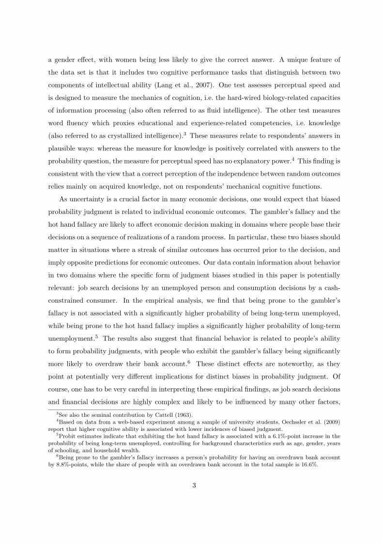
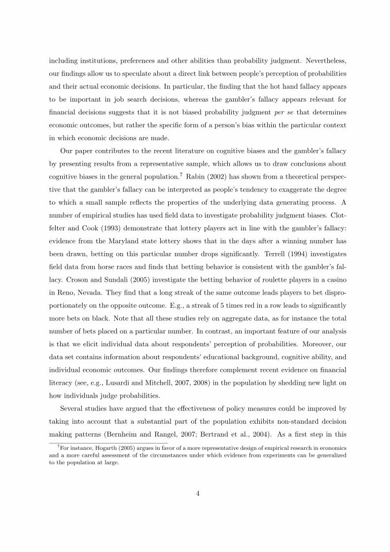
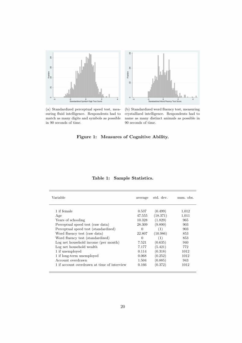
Sample statistics are shown in Table 1. About 53.7% of the sample are female, average
age is 47.6 years, and respondents have on average 10.3 years of schooling.9 The measures for9There are two types of high school in Germany, vocational and university-track. Individuals opting for the
vocational track leave school after 9 or 10 years and then typically go on to do an apprenticeship or vocational
6
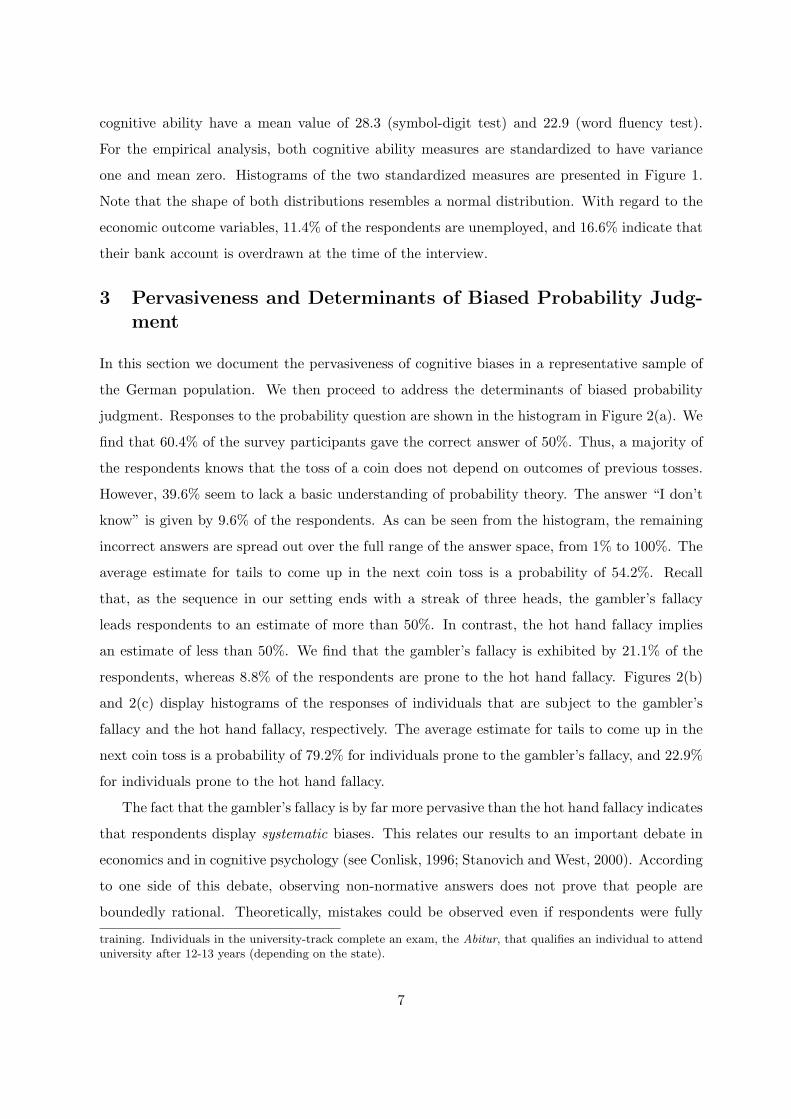
cognitive ability have a mean value of 28.3 (symbol-digit test) and 22.9 (word fluency test).
For the empirical analysis, both cognitive ability measures are standardized to have variance
one and mean zero. Histograms of the two standardized measures are presented in Figure 1.
Note that the shape of both distributions resembles a normal distribution. With regard to the
economic outcome variables, 11.4% of the respondents are unemployed, and 16.6% indicate that
their bank account is overdrawn at the time of the interview.
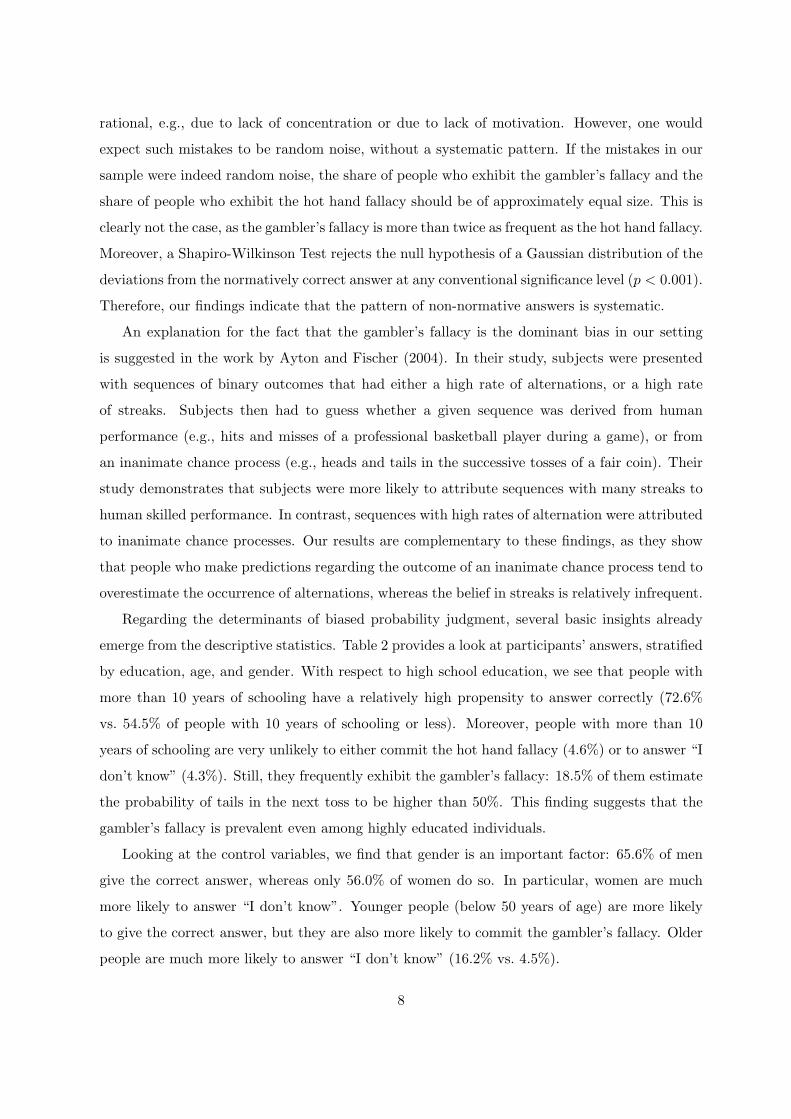
3 Pervasiveness and Determinants of Biased Probability Judg-ment
In this section we document the pervasiveness of cognitive biases in a representative sample of
the German population. We then proceed to address the determinants of biased probability
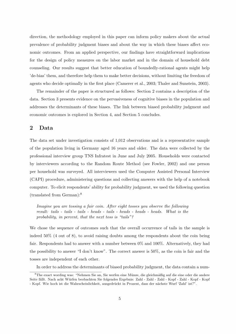
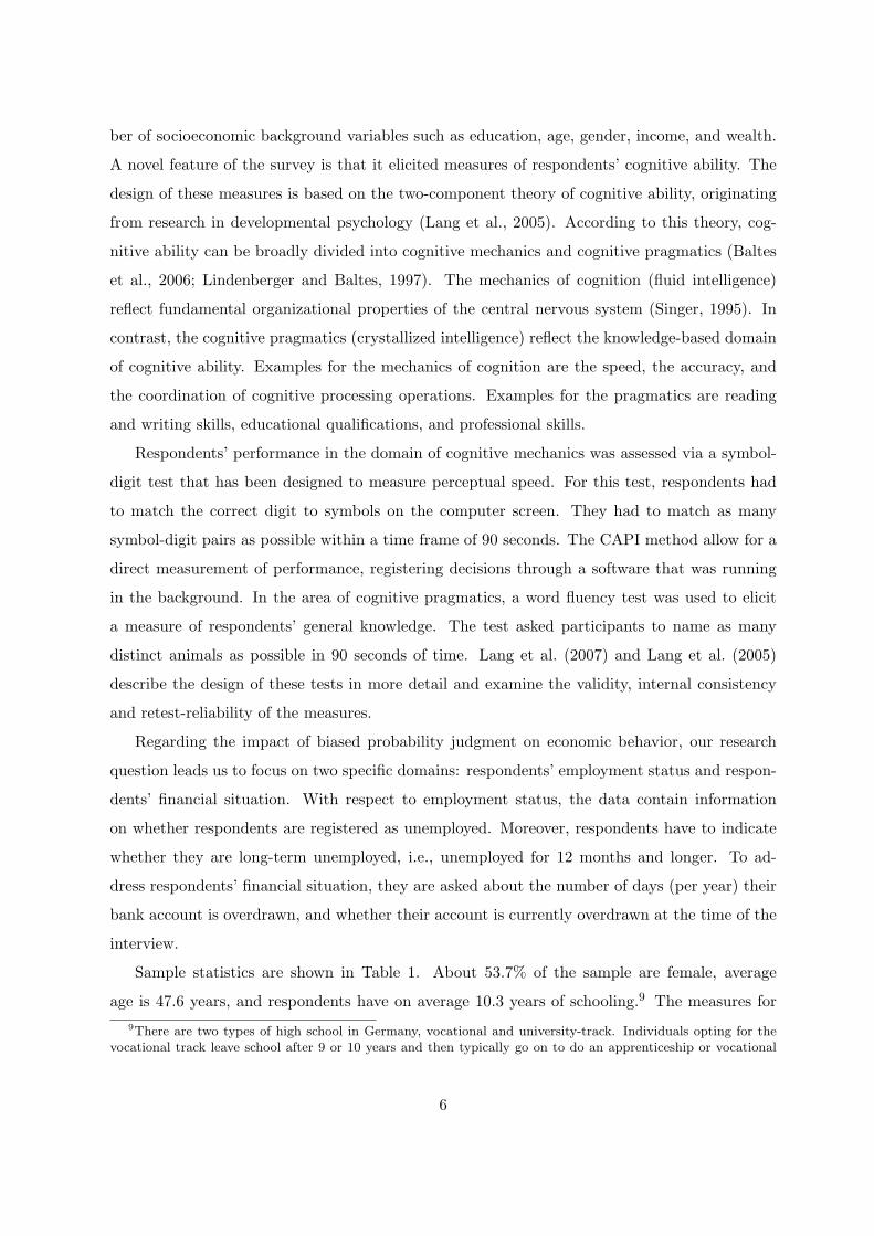
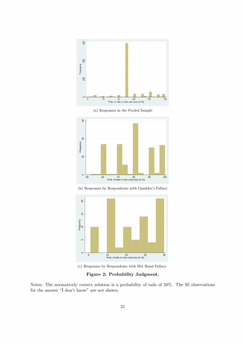
judgment. Responses to the probability question are shown in the histogram in Figure 2(a). We
find that 60.4% of the survey participants gave the correct answer of 50%. Thus, a majority of
the respondents knows that the toss of a coin does not depend on outcomes of previous tosses.
However, 39.6% seem to lack a basic understanding of probability theory. The answer “I don’t
know” is given by 9.6% of the respondents. As can be seen from the histogram, the remaining
incorrect answers are spread out over the full range of the answer space, from 1% to 100%. The
average estimate for tails to come up in the next coin toss is a probability of 54.2%. Recall
that, as the sequence in our setting ends with a streak of three heads, the gambler’s fallacy
leads respondents to an estimate of more than 50%. In contrast, the hot hand fallacy implies
an estimate of less than 50%. We find that the gambler’s fallacy is exhibited by 21.1% of the
respondents, whereas 8.8% of the respondents are prone to the hot hand fallacy. Figures 2(b)
and 2(c) display histograms of the responses of individuals that are subject to the gambler’s
fallacy and the hot hand fallacy, respectively. The average estimate for tails to come up in the
next coin toss is a probability of 79.2% for individuals prone to the gambler’s fallacy, and 22.9%
for individuals prone to the hot hand fallacy.
The fact that the gambler’s fallacy is by far more pervasive than the hot hand fallacy indicates
that respondents display systematic biases. This relates our results to an important debate in
economics and in cognitive psychology (see Conlisk, 1996; Stanovich and West, 2000). According
to one side of this debate, observing non-normative answers does not prove that people are
boundedly rational. Theoretically, mistakes could be observed even if respondents were fully
training. Individuals in the university-track complete an exam, the Abitur, that qualifies an individual to attenduniversity after 12-13 years (depending on the state).
7
rational, e.g., due to lack of concentration or due to lack of motivation. However, one would
expect such mistakes to be random noise, without a systematic pattern. If the mistakes in our
sample were indeed random noise, the share of people who exhibit the gambler’s fallacy and the
share of people who exhibit the hot hand fallacy should be of approximately equal size. This is
clearly not the case, as the gambler’s fallacy is more than twice as frequent as the hot hand fallacy.
Moreover, a Shapiro-Wilkinson Test rejects the null hypothesis of a Gaussian distribution of the
deviations from the normatively correct answer at any conventional significance level (p < 0.001).
Therefore, our findings indicate that the pattern of non-normative answers is systematic.
An explanation for the fact that the gambler’s fallacy is the dominant bias in our setting
is suggested in the work by Ayton and Fischer (2004). In their study, subjects were presented
with sequences of binary outcomes that had either a high rate of alternations, or a high rate
of streaks. Subjects then had to guess whether a given sequence was derived from human
performance (e.g., hits and misses of a professional basketball player during a game), or from
an inanimate chance process (e.g., heads and tails in the successive tosses of a fair coin). Their
study demonstrates that subjects were more likely to attribute sequences with many streaks to
human skilled performance. In contrast, sequences with high rates of alternation were attributed
to inanimate chance processes. Our results are complementary to these findings, as they show
that people who make predictions regarding the outcome of an inanimate chance process tend to
overestimate the occurrence of alternations, whereas the belief in streaks is relatively infrequent.
Regarding the determinants of biased probability judgment, several basic insights already
emerge from the descriptive statistics. Table 2 provides a look at participants’ answers, stratified
by education, age, and gender. With respect to high school education, we see that people with
more than 10 years of schooling have a relatively high propensity to answer correctly (72.6%
vs. 54.5% of people with 10 years of schooling or less). Moreover, people with more than 10
years of schooling are very unlikely to either commit the hot hand fallacy (4.6%) or to answer “I
don’t know” (4.3%). Still, they frequently exhibit the gambler’s fallacy: 18.5% of them estimate
the probability of tails in the next toss to be higher than 50%. This finding suggests that the
gambler’s fallacy is prevalent even among highly educated individuals.
Looking at the control variables, we find that gender is an important factor: 65.6% of men
give the correct answer, whereas only 56.0% of women do so. In particular, women are much
more likely to answer “I don’t know”. Younger people (below 50 years of age) are more likely
to give the correct answer, but they are also more likely to commit the gambler’s fallacy. Older
people are much more likely to answer “I don’t know” (16.2% vs. 4.5%).
8

In the following regression analysis we test whether these determinants are statistically signif-
icant and robust to controlling for background characteristics. Table 3 presents probit estimates
with the dependent variable being equal to 1 if a respondent gives the correct answer of 50%.10
It turns out that the effect of schooling is large and significant: an additional year of schooling
is related to an increase in the probability of giving the correct answer of about 4.5 percentage
points (p < 0.01), controlling for cognitive ability. As the baseline of correct answers in the total
sample is 60.4%, this effect is quite sizeable. For the cognitive ability measures, we see that the
coefficient for the word fluency measure is large and significant, whereas the coefficient for the
perceptual speed measure is small and insignificant. These results suggest that the cognitive
pragmatics (general knowledge) have a decisive impact on giving the correct answer, whereas me-
chanical cognitive ability (perceptual speed, quick comprehension) is not relevant to answering
the question at hand. Given that the task does not allude to computational skills but is rather
testing knowledge that is part of general education, this is a plausible finding. Regarding the
control variables, we find a significant gender effect that persists even if we include age, cognitive
ability and years of schooling in the regression. According to the estimates, the probability of
giving the correct answer is almost 10 percentage points lower for women (p < 0.01).11
To address the interplay between the nature of participants’ cognitive biases and their back-
ground characteristics in more detail, we estimate multinomial logit and multinomial probit
models (Table 4). These regression methods allow us to determine whether the differences
between the separate answer categories are statistically significant. The dependent variable in-
dicates in which of the four categories a respondents’ answer is located: either it is correct, or
it is consistent with either the gambler’s fallacy or the hot hand fallacy, or the respondent an-
swered “I don’t know”. In the estimations, the reference group consists of those respondents who
answered the probability question correctly. This allows us to analyze which factors determine
whether a respondent exhibits a particular bias. The estimates confirm our earlier descriptive
analysis. For instance, the effect of years of schooling is highly significant: schooling reduces the
probability of making a mistake. This finding holds for each of the three possible mistakes, be it
the hot hand fallacy, the gambler’s fallacy, or the answer “I don’t know”. Remarkably, the effect10For simplicity, answering “I don’t know” is categorized as a wrong answer in these regressions. If we exclude
these observations from the analysis (i.e., categorize them as missing), the results are very similar. The coefficientsfor gender and years of schooling remain highly significant, only the word fluency measure turns out to beinsignificant.
11A similar gender effect has been shown by Charness and Levin (2005), who conducted a laboratory experimentto test under which circumstances individual behavior in a probabilistic decision making task is consistent withstandard economic theory. Our data allows us to show in a representative sample that the gender effect persistswhen we control for background characteristics.
9
of schooling is quite asymmetric: Whereas more schooling protects people from committing the
hot hand fallacy (coefficient -0.293, p < 0.01 when controlling for word fluency in the multi-
nomial logit estimations; coefficient -0.294, p < 0.01 when controlling for perceptual speed in
the multinomial logit estimations), its impact on averting the gambler’s fallacy is considerably
weaker (coefficients of -0.122, p = 0.02 and -0.144, p < 0.01, respectively). This is in line with
the descriptive evidence which showed that the gambler’s fallacy is quite common among highly
educated individuals, whereas the hot hand fallacy is mostly confined to respondents with 10
years of schooling or less. With regard to the control variables, we find that women and older
people are significantly more likely to answer “I don’t know”.
Taken together, our findings regarding the determinants of biased probability judgment all
point in the same direction: more schooling increases the likelihood that a respondent gives the
correct answer in the probability task. From a policy perspective, it is important to stress that
schooling has an effect on probability judgment beyond the impact that works through cognitive
abilities. A competing hypothesis would be that the only determinant of probability judgment
is cognitive ability, which also related to the amount of schooling a given person obtains. To
avoid this confound, we controlled in all regressions for cognitive ability by including measures of
respondents’ word fluency and perceptual speed. As the coefficient on years of schooling remains
highly significant, the estimates suggest that schooling directly affects people’s capability for
probability judgment.
4 Economic Outcomes and Biased Probability Judgment
Uncertainty is a crucial factor in many economic decisions. One would therefore expect that
biased probability judgment can have a detrimental effect on individual economic outcomes. We
investigate two domains in which decisions are of a nature that closely resembles the structure of
our probability judgment task: job search decisions by an unemployed person and consumption
decisions by a cash-constrained consumer. In the following, we first develop predictions of how
the gambler’s fallacy and the hot hand fallacy might affect decision making in these domains.
In a second step we investigate the hypotheses in our data set.
4.1 Behavioral Predictions
The biases that are in the focus of this paper are likely to affect economic decision making in
domains where agents base their decisions on a sequence of realizations of a random process.
A straightforward translation of this environment can be found in the domain of job search.
10
As a thought experiment, assume that a person is looking for a job and sends out a number
of applications. The relevant sequence of random outcomes consists then of the reactions that
the job seeker receives on his applications: they can be either negative (a rejection) or positive
(a job offer). After observing the realization of a sequence of outcomes, the job seeker has to
decide whether to continue his search for a job or not.
Of course, many factors can play a role in the job finding process. For instance, the institu-
tional environment, the particular skills of a job-seeker, as well as his previous work experience
might have a large influence on success in the labor market. Still, our approach allows us to
speculate about an additional influence that might play a role on top of these factors: the im-
pact of a job-seeker’s perception of probabilities on actual job search behavior. Given the nature
of the cognitive biases we investigate, we are interested mainly in situations where a streak of
similar outcomes has occurred prior to the decision. Consider the case in which a job seeker
has received a streak of rejections, and suppose that, as is standard in search models, search
outcomes are independent from each other. The probability of generating a job offer is only
related to search intensity, a choice variable of the searcher. Then, the two probability judgment
biases, gambler’s fallacy and hot hand fallacy, would imply different predictions: a person who is
prone to the gambler’s fallacy should believe that the streak of rejections is going to end, which
implies that a job offer has now become more likely. As a consequence, the unemployed will be
encouraged to continue his search for a job. In contrast, a person who is prone to the hot hand
fallacy is going to believe that the streak of rejections is likely to continue. Given this belief,
the worker will become discouraged and may give up his search for a job altogether. One would
therefore predict that job-seekers who are prone to the gambler’s fallacy face a high probability
of leaving unemployment. In contrast, the hot hand fallacy can lead to prolonged unemployment
by biasing the job-seeker’s beliefs about his job finding probability such that they become too
pessimistic.12 Note that, due to the need for a streak of rejections to occur, our prediction is
unlikely to affect persons who just became unemployed a short while ago. Rather, we would
expect the detrimental effect of the hot hand fallacy to play a role for job seekers who have been
unemployed for a long time.13
12In the opposite case (in which a streak of job offers has occurred) the theoretical predictions are less clear.Here, it is very likely that both a gambler’s fallacy type and a hot hand fallacy type are going to accept one ofthe job offers and therefore stop searching for a job.
13The assumption of a stationary job finding probability, with job offers arriving at a fixed Poisson rate –and therefore the independence of subsequent realizations of job search outcomes – is standard in the searchliterature. Exceptions are papers considering inherently non-stationary subjective job finding probabilities in anenvironment in which there is employer stigma, or in which the unemployed have imperfect information abouttheir stationary job finding probability and update their subjective beliefs about this probability. In this context,
11
Another domain where biased probability judgment might have a substantial effect on eco-
nomic behavior is in the domain of consumption decisions. Assume that a cash-constrained
consumer has to decide whether to make a large purchase that exceeds the amount of funds
that is currently available in his bank account. Thus, in order to make the purchase, the con-
sumer would have to overdraw his account. In this context, the sequence of random outcomes
on which the decision is based can be thought of as unexpected idiosyncratic income shocks
that are either positive (e.g., finding a bank note on the sidewalk, winning money in a game
of poker with friends) or negative (e.g., receiving a speeding ticket, having a bill to pay that is
higher than anticipated). The consumption decision will then depend on the belief whether it
is likely that a positive income shock occurs in the near future. If this probability is high, it
is optimal to overdraw the bank account for the short period until the positive income shock
realizes. If, instead, this probability is low, it is optimal to postpone the purchase until it can
be made without overdrawing the account.
Again, we are interested in a situation where the decision maker has experienced a streak of
similar outcomes. Consider the case in which a streak of negative income shocks has occurred.
The probability judgment biases lead to the following behavioral predictions: if the consumer is
prone to the gambler’s fallacy, he will have the belief that the streak of negative income shocks
is likely to end, such that a positive income shock will realize with a high probability in the near
future. Thus, his inclination to overdraw the bank account in order to make the purchase will
be high. In contrast, the hot hand fallacy will lead to the opposite prediction: if the consumer
believes that the streak of negative income shocks is likely to continue, he will refrain from
overdrawing his account and will not make the purchase.14 In sum, a person who is prone to
the gambler’s fallacy is predicted to be more likely to have an overdrawn bank account, as the
biased belief that a positive income shock is “due” can lead to persistent household debt. By
the unemployed’s personal job search history (i.e., past realizations) matters and may lead to a discouraged workereffect, see Falk (2006a, 2006b). These cases would leave the hypotheses arising from biased probability judgmentunaffected. For instance, even in a model with learning about the job finding probability, one would predictthat a hot hand fallacy type reduces search intensity faster than people without bias in probability judgment, orgambler’s fallacy types, after a streak of negative search outcomes for a given job finding rate. This is because hothand fallacy types overvalue the information content of a streak of negative outcomes since they would predictfuture outcomes to be more likely to be negative than they really are. Thus, although updating might be thechannel through which searchers become long-term unemployed, the underlying reason for hot hand fallacy typesto become discouraged faster is their biased probability judgment.
14Predictions in the opposite case (in which a streak of positive income shocks has occurred) are ambiguous: ifthe consumer is prone to the hot hand fallacy, he will believe that the positive income shocks are going to continueand he will decide to make the large purchase. If the respondent is prone to the gambler’s fallacy instead, he willexpect that a negative income shock is likely to occur in the near future. Still, if the streak of positive incomeshocks has led to a large amount of funds available in his account, he might nevertheless make the purchase.
12
contrast, a person who is prone to the hot hand fallacy will be less likely to have an overdrawn
bank account.
4.2 Empirical Results
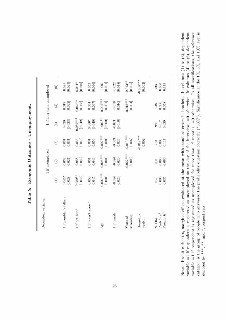
To test the predictions regarding employment status with our data, we run two sets of regressions.
First, we estimate a probit model in which the dependent variable is a dummy equal to one if the
respondent is registered as unemployed at the time of the interview. In a second set of regressions,
the dependent variable is an indicator for whether the respondent is long-term unemployed, i.e.,
registered as unemployed for 12 months or more. As explanatory variables, we include dummies
for the observed cognitive biases: the gambler’s fallacy, the hot hand fallacy, and the answer
“I don’t know”. The reference group consists therefore of those respondents who answered the
probability judgment task correctly. Results from regressions with the unemployment dummy
as dependent variable are presented in Table 5. In column (1) we control only for age and
gender and find that both the hot hand dummy and the gambler’s fallacy dummy are positive
and weakly significant. Adding controls for education and for wealth renders both coefficients
insignificant, see columns (2) and (3).
In light of the hypotheses described before, our analysis next turns to persons who have
been looking for a job for an extended period of time. Columns (4) to (6) present results from
regressions where the dependent variable is a dummy equal to one for respondents who are long-
term unemployed. The explanatory variables are the same variables as before. Our estimates
show that, controlling for age and gender, the hot hand fallacy is positive and significant at the
1%-level. Thus, the results are consistent with the behavioral predictions regarding the effect
of the hot hand fallacy on long-term unemployment. If, in addition, we control for respondents’
educational background, the coefficient for the hot hand fallacy remains significant at the 5%-
level. Even if we control for education and wealth, the coefficient for the hot hand fallacy dummy
remains significant at the 10%-level and the marginal effect indicates that the probability of
being long-term unemployed is increased by 6.1%-points.15 Given that the baseline of long-term
unemployment in the sample is 6.8%, this is a considerable effect. We therefore conclude that
our predictions regarding the detrimental effect of the hot hand fallacy are supported in case of
long-term unemployed job seekers. Moreover, we find for all specifications that the gambler’s
fallacy has no significant effect on employment status, which is again in line with our predictions.15We deliberately chose not to control for household income in the unemployment regressions, in order to avoid
endogeneity problems.
13
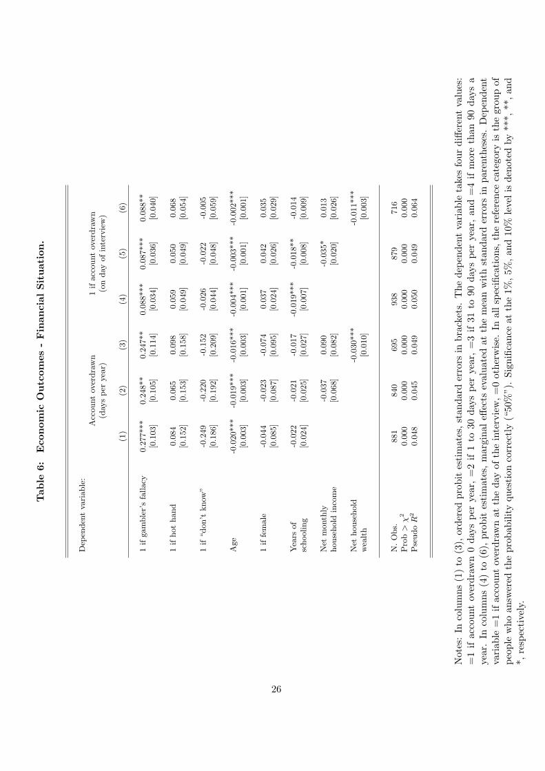
Next, we empirically test the predictions regarding consumption decisions of cash-constrained
consumers. To this aim, we analyze the interplay of probability judgment biases and the decision
to overdraw one’s bank account. In a first set of regressions, the dependent variable indicates
how many days per year a respondent’s bank account is overdrawn. The variable can take on
four distinct values, as the set of possible responses consisted of four intervals (0 days, 1 to 30, 31
to 90, more than 90 days). As explanatory variables we include again the dummies for whether a
person exhibits a bias in probability judgment, with the reference group being those respondents
who gave the correct answer to the probability task. Results of ordered probit regressions are
presented in columns (1) to (3) of Table 6. The estimates show that the dummy for whether a
respondent is prone to the gambler’s fallacy is positive and significant at the 1%-level even when
controlling for age, gender, and education. Adding controls for net household income and net
household wealth leaves the coefficient virtually unchanged and significant at the 5%-level. This
is in line with the behavioral prediction: people who are prone to the gambler’s fallacy have a
higher number of days per year on which their bank account is overdrawn.
As it might be relatively complicated for respondents to assess the number of days per year
on which their account is in the negative, the survey also included the straightforward question
of whether a person’s account was overdrawn at the time of the interview. A look at the raw
data reveals large effects: out of the respondents who answer the probability question correctly,
14.3% have an overdrawn bank account. In contrast, this figure is 24.5% among the group of
people who are prone to the gambler’s fallacy. Results of a probit estimation with this simple
measure as dependent variable are presented in columns (4) to (6). The estimates are very
similar to our earlier findings: in most specifications, the coefficient on the gambler’s fallacy
dummy is positive and significant at the 1%-level. The marginal effects indicate that being
prone to the gambler’s fallacy increases the probability of having an overdrawn bank account
by about 8.8%-points (p = 0.020), controlling for age, gender, education, income, and wealth.
This is a sizeable effect, as the share of respondents with an overdrawn bank account is 16.6%
in the total sample. Again, these findings are in line with the predictions: the gambler’s fallacy
has a substantial impact on consumers’ decision to overdraw their bank account.
Taken together, our results are consistent with the behavioral hypotheses that were developed
in Section 4.1. In particular, we find that the gambler’s fallacy affects financial decision making,
whereas the hot hand fallacy has an impact on job search decisions. These findings suggest that
it is not biased probability judgment per se that affects economic outcomes. Rather, depending
on the context in which economic decisions are made, the specific form of a person’s probability
14
judgment bias might play a decisive role.
5 Conclusion
This paper addressed three closely related research questions. First, it investigated people’s
ability to make simple probability judgments. For this purpose, we used a specifically designed
probability judgment question that was administered to a representative sample of the German
adult population. The results showed that more than a third of the respondents was unable to
answer the probability question correctly, indicating that a substantial part of the population
has difficulties with making simple probability judgments. Among the incorrect answers, by
far the most frequent bias was the gambler’s fallacy, i.e., the tendency to overestimate the
occurrence of alternations in random sequences. Second, we addressed the determinants of
biased probability judgment. Our results have shown that education (years of schooling) and
a knowledge-based measure of cognitive ability are positively related to performance in the
probability judgment task. The third part of the paper explored the relation between the
observed probability judgment patterns and respondents’ behavior in two domains: job search
and financial decision making. The hot hand fallacy, i.e., the tendency to overestimate the
occurrence of streaks in random sequences, was shown to be significantly related to a higher
probability of being long-term unemployed. In contrast, the gambler’s fallacy was found to be
associated with a higher probability of overdrawing one’s bank account.
If our interpretation of the results, namely that biased probability judgment is likely to
translate into inferior economic outcomes, is correct, our finding regarding the impact of school-
ing are of relevance from a policy perspective. Our estimates have shown that schooling has a
large and significant impact on reducing people’s cognitive biases. The fact that the estimates
were positive and significant even when controlling for cognitive ability suggests that the knowl-
edge obtained in school mitigates probability judgment biases in a direct way. Thus, it may
be worthwhile to put a stronger focus on teaching simple probabilistic reasoning already in the
early grades of high school. More generally, an increased dissemination of basic knowledge about
random processes might help people to make better decisions in the economic domains of life.
From an applied perspective, our findings have straightforward implications for the design
of policy measures, emphasizing the role of debiasing of decision makers. With respect to labor
market policy, our results suggest that job centers should offer courses that teach job-seekers
about the probabilities that play a role in the application process. Rather than believing that
15
their future search success will be the outcome of a continued streak of unsuccessful applications,
job-seekers should understand that their job finding probabilities depend on the overall labor
market conditions in a particular occupation or region, and that the outcome of a particular
application does not necessarily directly depend on earlier unsuccessful applications elsewhere.
Similar policy implications can be derived for the domain of household finances. Here, counselors
who give advice to over-indebted households could inform consumers who exhibit the gambler’s
fallacy that they should avoid to overestimate the probability of a positive income shock to occur
in the near future.
Of course, the analysis in this paper has limitations. For instance, we were not able to
identify the exact channels through which a cognitive bias influences behavior. While some
of our results are in line with the gambler’s fallacy being a sign of over-optimism (as in the
overdrawn bank account measure), this behavior might as well be related to time-inconsistent
preferences or other cognitive biases in financial decision making (see, e.g., Laibson, 1997, or
Stango and Zinman, 2009). A promising direction for future research is the combination of
incentivized measures of people’s time and risk preferences with measures of biased probability
judgment, in order to identify the channels through which biased probability judgment affects
economic behavior.
16
References
Ayton, P. and Fischer, I. (2004), ‘The hot hand fallacy and the gambler’s fallacy: Two faces ofsubjective randomness?’, Memory & Cognition 32(8), 1369–1378.
Baltes, P. B., Lindenberger, U. and Staudinger, U. M. (2006), Life span theory in developmentalpsychology, in W. Damon and R. M. Lerner, eds, ‘Handbook of child psychology: Vol. 1.Theoretical models of human development (6th ed.)’, Wiley, New York, pp. 569–664.
Bernheim, B. D. and Rangel, A. (2007), Behavioral public economics: Welfare and policy anal-ysis with non-standard decision-makers, in P. Diamond and H. Vartiainen, eds, ‘BehavioralEconomics and its Applications’, Princeton University Press.
Bertrand, M., Mullainathan, S. and Shafir, E. (2004), ‘A behavioral-economics view of poverty’,American Economic Review, Papers and Proceedings 94, 419–423.
Camerer, C., Issacharoff, S., Loewenstein, G., O’Donoghue, T. and Rabin, M. (2003), ‘Regulationfor Conservatives: Behavioral Economics and the Case for “Asymmetric Paternalism”’,University of Pennsylvania Law Review 151(3), 1211–1254.
Cattell, R. B. (1963), ‘Theory of Fluid and Crystallized Intelligence: A Critical Experiment’,Journal of Educational Psychology 54(1), 1–22.
Charness, G. and Levin, D. (2005), ‘When optimal choices feel wrong: A laboratory study ofbayesian updating, complexity, and affect’, American Economic Review 95, 1300–1309.
Clotfelter, C. T. and Cook, P. J. (1993), ‘The “gambler’s fallacy” in lottery play’, ManagementScience 39, 1521–1525.
Conlisk, J. (1996), ‘Why bounded rationality?’, Journal of Economic Literature 34, 669–700.
Croson, R. and Sundali, J. (2005), ‘The gambler’s fallacy and the hot hand: Empirical datafrom casinos’, Journal of Risk and Uncertainty 30, 195–209.
Falk, A., Huffman, D. and Sunde, U. (2006a), ‘Do I Have What it Takes? Equilibrium Searchwith Type Uncertainty and Non-Participation’, IZA Discussion Paper No. 2531 .
Falk, A., Huffman, D. and Sunde, U. (2006b), ‘Self-Confidence and Search’, IZA DiscussionPaper No. 2525 .
Fowler, F. J. (2002), Survey Research Methods, Sage Publications, London.
Gilovich, T., Vallone, R. and Tversky, A. (1985), ‘The hot hand in basketball: On the misper-ception of random sequences’, Cognitive Psychology 17, 295–314.
17
Grether, D. M. (1980), ‘Bayes rule as a descriptive model: The representativeness heuristic’,Quarterly Journal of Economics 95(3), 537–557.
Hogarth, R. M. (2005), ‘The challenge of representative design in psychology and economics’,Journal of Economic Methodology 12(2), 253–263.
Laibson, D. (1997), ‘Golden Eggs and Hyperbolic Discounting’, The Quarterly Journal of Eco-nomics 112(2), 443–477.
Lang, F. R., Hahne, D., Gymbel, S., Schropper, S. and Lutsch, K. (2005), Erfassung des kogni-tiven Leistungspotenzials und der “Big Five” mit Computer-Assited-Personal-Interviewing(CAPI): Zur Reliabilitat und Validitat zweier ultrakurzer Tests und des BFI-S. DIW Re-search Notes 9/2005, DIW Berlin.
Lang, F. R., Weiss, D., Stocker, A. and von Rosenbladt, B. (2007), ‘Assessing Cognitive Capac-ities in Computer-Assited Survey Research: Two Ultra-Short Tests of Intellectual Abilityin the German Socio-Economic Panel (SOEP)’, Schmollers Jahrbuch 127(1), 183–192.
Laplace, P. (1820), Philosophical Essays on Probabilities, Dover, New York. (translated by F.W.Truscott and F. L. Emory, 1951).
Lindenberger, U. and Baltes, P. B. (1997), ‘Intellectual functioning in old and very old age:Cross-sectional results from the berlin aging study’, Psychology and Aging 12(3), 410–432.
Lusardi, A. and Mitchell, O. S. (2007), ‘Baby Boomer Retirement Security: The Roles of Plan-ning, Financial Literacy, and Housing Wealth’, Journal of Monetary Economics 54, 205–224.
Lusardi, A. and Mitchell, O. S. (2008), ‘Planning and Financial Literacy: How Do WomenFare?’, American Economic Review 98(2), 413–417.
Oechssler, J., Roider, A. and Schmitz, P. (2009), ‘Cognitive Abilities and Behavioral Biases’,Journal of Economic Behavior and Organization, forthcoming .
Rabin, M. (2002), ‘Inference by Believers in the Law of Small Numbers’, Quarterly Journal ofEconomics 117(3), 775–816.
Singer, W. (1995), ‘Development and plasticity of cortical processing architectures’, Science270, 758–764.
Stango, V. and Zinman, D. (2009), ‘Exponential Growth Bias and Household Finance’, Journalof Finance, forthcoming .
Stanovich, K. E. and West, R. F. (2000), ‘Individual differences in reasoning: Implications forthe rationality debate?’, Behavioral and Brain Sciences 23, 645–726.
18
Terrell, D. (1994), ‘A test of the gambler’s fallacy: Evidence from pari-mutuel games’, Journalof Risk and Uncertainty 8, 309–317.
Thaler, R. H. and Sunstein, C. R. (2003), ‘Libertarian Paternalism’, The American EconomicReview 93(2), 175–179.
Tversky, A. and Kahneman, D. (1971), ‘Belief in the law of small numbers’, PsychologicalBulletin 2, 105–110.
19
0.0
1.0
2.0
3.0
4F
ract
ion
−4 −2 0 2 4Standardized Symbol−Digit Test Score
(a) Standardized perceptual speed test, mea-suring fluid intelligence. Respondents had tomatch as many digits and symbols as possiblein 90 seconds of time.
0.0
2.0
4.0
6F
ract
ion
−4 −2 0 2 4Standardized Word Fluency Test Score
(b) Standardized word fluency test, measuringcrystallized intelligence. Respondents had toname as many distinct animals as possible in90 seconds of time.
Figure 1: Measures of Cognitive Ability.
Table 1: Sample Statistics.
Variable average std. dev. num. obs.
1 if female 0.537 (0.499) 1,012Age 47.555 (18.371) 1,011Years of schooling 10.328 (1.829) 965Perceptual speed test (raw data) 28.309 (9.890) 903Perceptual speed test (standardized) 0 (1) 903Word fluency test (raw data) 22.807 (10.986) 853Word fluency test (standardized) 0 (1) 853Log net household income (per month) 7.521 (0.635) 940Log net household wealth 7.177 (5.421) 7721 if unemployed 0.114 (0.318) 10121 if long-term unemployed 0.068 (0.252) 1012Account overdrawn 1.504 (0.885) 9431 if account overdrawn at time of interview 0.166 (0.372) 1012
20
(a) Responses in the Pooled Sample
020
4060
Fre
quen
cy
50 60 70 80 90 100Prob. of tails in next coint toss (in %)
(b) Responses by Respondents with Gambler’s Fallacy
05
1015
20F
requ
ency
0 10 20 30 40Prob. of tails in next coint toss (in %)
(c) Responses by Respondents with Hot Hand Fallacy
Figure 2: Probability Judgment.
Notes: The normatively correct solution is a probability of tails of 50%. The 95 observationsfor the answer “I don’t know” are not shown.
21
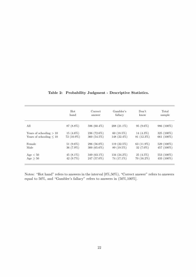
Table 2: Probability Judgment - Descriptive Statistics.
Hot Correct Gambler’s Don’t Totalhand answer fallacy know sample
All 87 (8.8%) 596 (60.4%) 208 (21.1%) 95 (9.6%) 986 (100%)
Years of schooling > 10 15 (4.6%) 236 (72.6%) 60 (18.5%) 14 (4.3%) 325 (100%)Years of schooling ≤ 10 72 (10.9%) 360 (54.5%) 148 (22.4%) 81 (12.3%) 661 (100%)
Female 51 (9.6%) 296 (56.0%) 119 (22.5%) 63 (11.9%) 529 (100%)Male 36 (7.9%) 300 (65.6%) 89 (19.5%) 32 (7.0%) 457 (100%)
Age < 50 45 (8.1%) 349 (63.1%) 134 (24.2%) 25 (4.5%) 553 (100%)Age ≥ 50 42 (9.7%) 247 (57.0%) 74 (17.1%) 70 (16.2%) 433 (100%)
Notes: “Hot hand” refers to answers in the interval [0%,50%), “Correct answer” refers to answersequal to 50%, and “Gambler’s fallacy” refers to answers in (50%,100%].
22
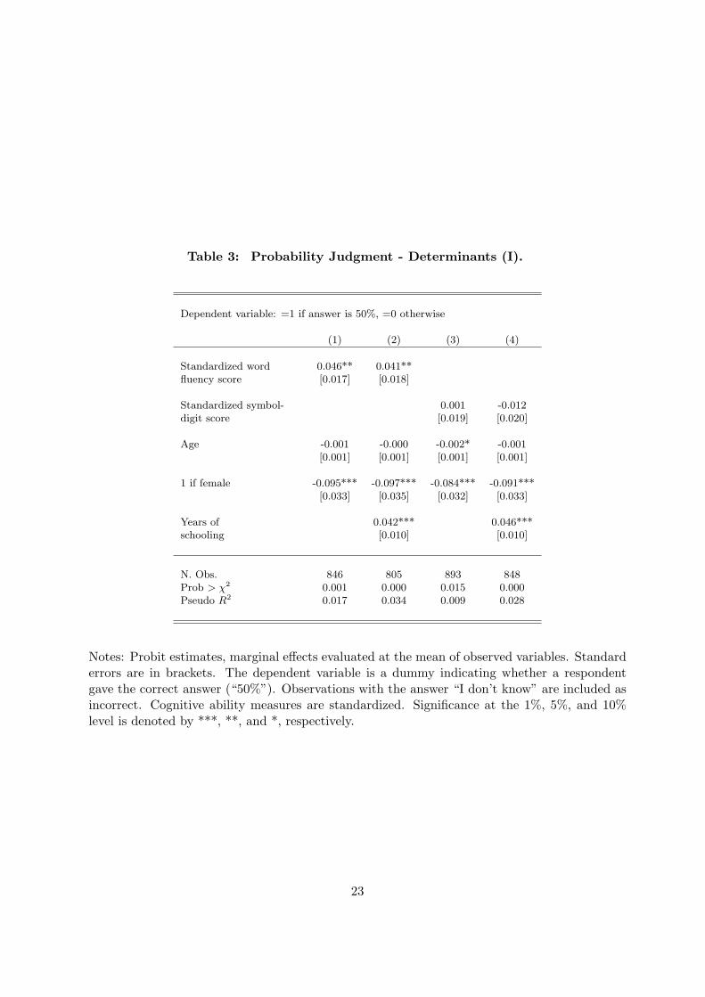
Table 3: Probability Judgment - Determinants (I).
Dependent variable: =1 if answer is 50%, =0 otherwise
(1) (2) (3) (4)
Standardized word 0.046** 0.041**fluency score [0.017] [0.018]
Standardized symbol- 0.001 -0.012digit score [0.019] [0.020]
Age -0.001 -0.000 -0.002* -0.001[0.001] [0.001] [0.001] [0.001]
1 if female -0.095*** -0.097*** -0.084*** -0.091***[0.033] [0.035] [0.032] [0.033]
Years of 0.042*** 0.046***schooling [0.010] [0.010]
N. Obs. 846 805 893 848Prob > χ2 0.001 0.000 0.015 0.000Pseudo R2 0.017 0.034 0.009 0.028
Notes: Probit estimates, marginal effects evaluated at the mean of observed variables. Standarderrors are in brackets. The dependent variable is a dummy indicating whether a respondentgave the correct answer (“50%”). Observations with the answer “I don’t know” are included asincorrect. Cognitive ability measures are standardized. Significance at the 1%, 5%, and 10%level is denoted by ***, **, and *, respectively.
23
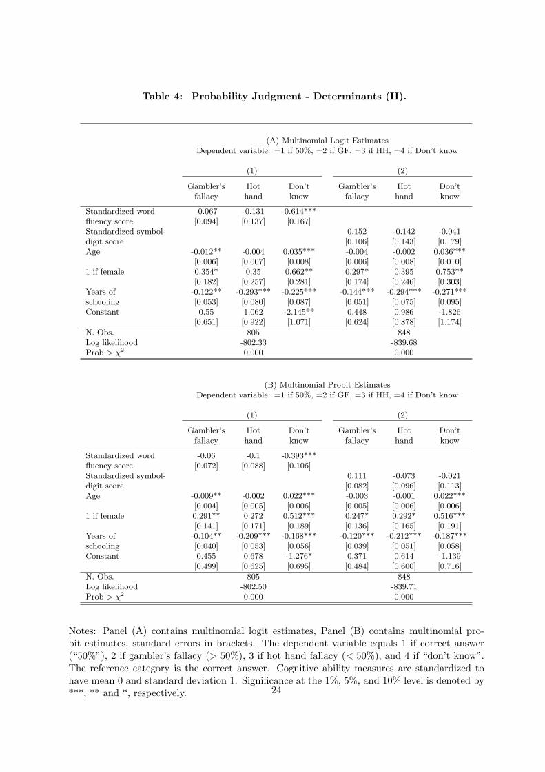
Table 4: Probability Judgment - Determinants (II).
(A) Multinomial Logit EstimatesDependent variable: =1 if 50%, =2 if GF, =3 if HH, =4 if Don’t know
(1) (2)
Gambler’s Hot Don’t Gambler’s Hot Don’tfallacy hand know fallacy hand know
Standardized word -0.067 -0.131 -0.614***fluency score [0.094] [0.137] [0.167]Standardized symbol- 0.152 -0.142 -0.041digit score [0.106] [0.143] [0.179]Age -0.012** -0.004 0.035*** -0.004 -0.002 0.036***
[0.006] [0.007] [0.008] [0.006] [0.008] [0.010]1 if female 0.354* 0.35 0.662** 0.297* 0.395 0.753**
[0.182] [0.257] [0.281] [0.174] [0.246] [0.303]Years of -0.122** -0.293*** -0.225*** -0.144*** -0.294*** -0.271***schooling [0.053] [0.080] [0.087] [0.051] [0.075] [0.095]Constant 0.55 1.062 -2.145** 0.448 0.986 -1.826
[0.651] [0.922] [1.071] [0.624] [0.878] [1.174]
N. Obs. 805 848Log likelihood -802.33 -839.68Prob > χ2 0.000 0.000
(B) Multinomial Probit EstimatesDependent variable: =1 if 50%, =2 if GF, =3 if HH, =4 if Don’t know
(1) (2)
Gambler’s Hot Don’t Gambler’s Hot Don’tfallacy hand know fallacy hand know
Standardized word -0.06 -0.1 -0.393***fluency score [0.072] [0.088] [0.106]Standardized symbol- 0.111 -0.073 -0.021digit score [0.082] [0.096] [0.113]Age -0.009** -0.002 0.022*** -0.003 -0.001 0.022***
[0.004] [0.005] [0.006] [0.005] [0.006] [0.006]1 if female 0.291** 0.272 0.512*** 0.247* 0.292* 0.516***
[0.141] [0.171] [0.189] [0.136] [0.165] [0.191]Years of -0.104** -0.209*** -0.168*** -0.120*** -0.212*** -0.187***schooling [0.040] [0.053] [0.056] [0.039] [0.051] [0.058]Constant 0.455 0.678 -1.276* 0.371 0.614 -1.139
[0.499] [0.625] [0.695] [0.484] [0.600] [0.716]
N. Obs. 805 848Log likelihood -802.50 -839.71Prob > χ2 0.000 0.000
Notes: Panel (A) contains multinomial logit estimates, Panel (B) contains multinomial pro-bit estimates, standard errors in brackets. The dependent variable equals 1 if correct answer(“50%”), 2 if gambler’s fallacy (> 50%), 3 if hot hand fallacy (< 50%), and 4 if “don’t know”.The reference category is the correct answer. Cognitive ability measures are standardized tohave mean 0 and standard deviation 1. Significance at the 1%, 5%, and 10% level is denoted by***, ** and *, respectively. 24
Tab
le5:
Eco
nom
icO
utc
omes
-U
nem
plo
ym
ent.
Dep
enden
tva
riable
:1
ifunem
plo
yed
1if
long-t
erm
unem
plo
yed
(1)
(2)
(3)
(4)
(5)
(6)
1if
gam
ble
r’s
fallacy
0.0
45*
0.0
32
0.0
31
0.0
29
0.0
19
0.0
25
[0.0
28]
[0.0
27]
[0.0
31]
[0.0
23]
[0.0
22]
[0.0
25]
1if
hot
hand
0.0
89**
0.0
58
0.0
56
0.0
89***
0.0
64**
0.0
61*
[0.0
46]
[0.0
43]
[0.0
46]
[0.0
42]
[0.0
38]
[0.0
40]
1if
“don’t
know
”0.0
50
0.0
31
0.0
31
0.0
60*
0.0
44
0.0
52
[0.0
45]
[0.0
43]
[0.0
53]
[0.0
40]
[0.0
37]
[0.0
46]
Age
-0.0
02***
-0.0
03***
-0.0
02***
-0.0
01**
-0.0
02***
-0.0
01
[0.0
01]
[0.0
01]
[0.0
01]
[0.0
00]
[0.0
01]
[0.0
01]
1if
fem
ale
-0.0
26
-0.0
26
-0.0
33
-0.0
21
-0.0
19
-0.0
22
[0.0
20]
[0.0
20]
[0.0
24]
[0.0
16]
[0.0
16]
[0.0
18]
Yea
rsof
-0.0
22***
-0.0
19***
-0.0
15***
-0.0
13**
schooling
[0.0
06]
[0.0
07]
[0.0
04]
[0.0
05]
House
hold
-0.0
12***
-0.0
08***
wea
lth
[0.0
02]
[0.0
02]
N.
Obs.
985
938
733
985
938
733
Pro
b>χ
20.0
00
0.0
00
0.0
00
0.0
17
0.0
00
0.0
00
Pse
udoR
20.0
35
0.0
66
0.1
17
0.0
29
0.0
58
0.1
19
Not
es:
Pro
bit
esti
mat
es,
mar
gina
leff
ects
eval
uate
dat
the
mea
nw
ith
stan
dard
erro
rsin
brac
kets
.In
colu
mns
(1)
to(3
),de
pend
ent
vari
able
=1
ifre
spon
dent
isre
gist
ered
asun
empl
oyed
onth
eda
yof
the
inte
rvie
w,
=0
othe
rwis
e.In
colu
mns
(4)
to(6
),de
pend
ent
vari
able
=1
ifre
spon
dent
isre
gist
ered
asun
empl
oyed
for
mor
eth
an12
mon
ths,
=0
othe
rwis
e.In
all
spec
ifica
tion
s,th
ere
fere
nce
cate
gory
isth
egr
oup
ofpe
ople
who
answ
ered
the
prob
abili
tyqu
esti
onco
rrec
tly
(“50
%”)
.Si
gnifi
canc
eat
the
1%,5
%,a
nd10
%le
veli
sde
note
dby
***,
**,
and
*,re
spec
tive
ly.
25
Tab
le6:
Eco
nom
icO
utc
omes
-F
inan
cial
Sit
uat
ion
.
Dep
enden
tva
riable
:A
ccount
over
dra
wn
1if
acc
ount
over
dra
wn
(day
sp
eryea
r)(o
nday
of
inte
rvie
w)
(1)
(2)
(3)
(4)
(5)
(6)
1if
gam
ble
r’s
fallacy
0.2
77***
0.2
48**
0.2
47**
0.0
88***
0.0
87***
0.0
88**
[0.1
03]
[0.1
05]
[0.1
14]
[0.0
34]
[0.0
36]
[0.0
40]
1if
hot
hand
0.0
84
0.0
65
0.0
98
0.0
59
0.0
50
0.0
68
[0.1
52]
[0.1
53]
[0.1
58]
[0.0
49]
[0.0
49]
[0.0
54]
1if
“don’t
know
”-0
.249
-0.2
20
-0.1
52
-0.0
26
-0.0
22
-0.0
05
[0.1
86]
[0.1
92]
[0.2
09]
[0.0
44]
[0.0
48]
[0.0
59]
Age
-0.0
20***
-0.0
19***
-0.0
16***
-0.0
04***
-0.0
03***
-0.0
02***
[0.0
03]
[0.0
03]
[0.0
03]
[0.0
01]
[0.0
01]
[0.0
01]
1if
fem
ale
-0.0
44
-0.0
23
-0.0
74
0.0
37
0.0
42
0.0
35
[0.0
85]
[0.0
87]
[0.0
95]
[0.0
24]
[0.0
26]
[0.0
29]
Yea
rsof
-0.0
22
-0.0
21
-0.0
17
-0.0
19***
-0.0
18**
-0.0
14
schooling
[0.0
24]
[0.0
25]
[0.0
27]
[0.0
07]
[0.0
08]
[0.0
09]
Net
month
ly-0
.037
0.0
90
-0.0
35*
0.0
13
house
hold
inco
me
[0.0
68]
[0.0
82]
[0.0
20]
[0.0
26]
Net
house
hold
-0.0
30***
-0.0
11***
wea
lth
[0.0
10]
[0.0
03]
N.
Obs.
881
840
695
938
879
716
Pro
b>χ
20.0
00
0.0
00
0.0
00
0.0
00
0.0
00
0.0
00
Pse
udoR
20.0
48
0.0
45
0.0
49
0.0
50
0.0
49
0.0
64
Not
es:
Inco
lum
ns(1
)to
(3),
orde
red
prob
ites
tim
ates
,sta
ndar
der
rors
inbr
acke
ts.
The
depe
nden
tva
riab
leta
kes
four
diffe
rent
valu
es:
=1
ifac
coun
tov
erdr
awn
0da
yspe
rye
ar,
=2
if1
to30
days
per
year
,=
3if
31to
90da
yspe
rye
ar,
and
=4
ifm
ore
than
90da
ysa
year
.In
colu
mns
(4)
to(6
),pr
obit
esti
mat
es,
mar
gina
leff
ects
eval
uate
dat
the
mea
nw
ith
stan
dard
erro
rsin
pare
nthe
ses.
Dep
ende
ntva
riab
le=
1if
acco
unt
over
draw
nat
the
day
ofth
ein
terv
iew
,=0
othe
rwis
e.In
alls
peci
ficat
ions
,the
refe
renc
eca
tego
ryis
the
grou
pof
peop
lew
hoan
swer
edth
epr
obab
ility
ques
tion
corr
ectl
y(“
50%
”).
Sign
ifica
nce
atth
e1%
,5%
,and
10%
leve
lis
deno
ted
by**
*,**
,and
*,re
spec
tive
ly.
26