Bias and Variance, Under-Fitting and Over-Fitting

Neural Computation : Lecture 9

© John A. Bullinaria, 2015

1. The Computational Power of MLPs

2. Learning and Generalization Revisited

3. Statistical View of Neural Network Learning

4. Bias and Variance Decomposition

5. Under-fitting, Over-fitting and the Bias/Variance Trade-off

6. Preventing Under-fitting and Over-fitting

L9-2

Computational Power of MLPs

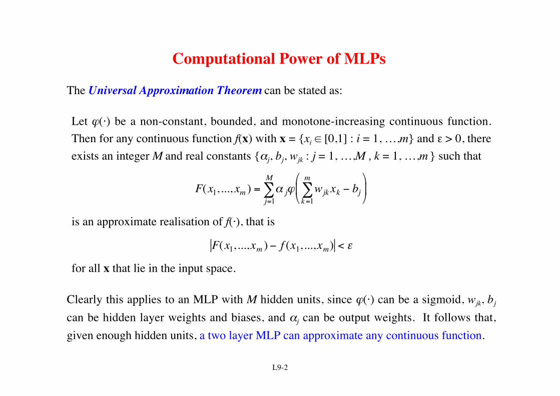
The Universal Approximation Theorem can be stated as:

Let ϕ(⋅) be a non-constant, bounded, and monotone-increasing continuous function.Then for any continuous function f(x) with x = {xi ∈ [0,1] : i = 1, …,m} and ε > 0, thereexists an integer M and real constants {αj, bj, wjk : j = 1, …,M , k = 1, …,m } such that

F(x1, ..., xm ) = α jj=1

M

∑ ϕ wjk xk − bjk=1

m

∑

is an approximate realisation of f(⋅), that is

F(x1, ...,xm ) − f (x1, ...,xm) < ε

for all x that lie in the input space.

Clearly this applies to an MLP with M hidden units, since ϕ(⋅) can be a sigmoid, wjk, bj

can be hidden layer weights and biases, and αj can be output weights. It follows that,given enough hidden units, a two layer MLP can approximate any continuous function.

L9-3

Learning and Generalization Revisited

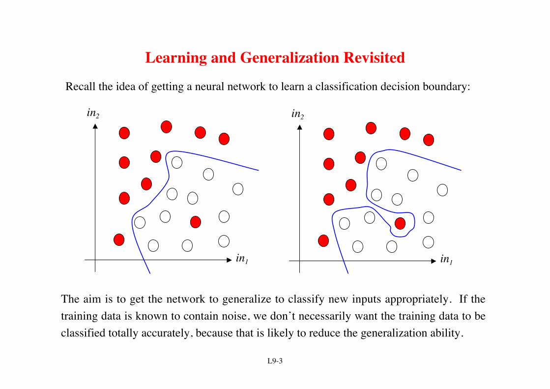
Recall the idea of getting a neural network to learn a classification decision boundary:

The aim is to get the network to generalize to classify new inputs appropriately. If thetraining data is known to contain noise, we don’t necessarily want the training data to beclassified totally accurately, because that is likely to reduce the generalization ability.

in1

in2

in1

in2

L9-4

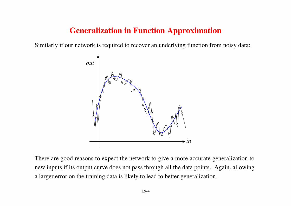
Generalization in Function ApproximationSimilarly if our network is required to recover an underlying function from noisy data:

There are good reasons to expect the network to give a more accurate generalization tonew inputs if its output curve does not pass through all the data points. Again, allowinga larger error on the training data is likely to lead to better generalization.

out

in

L9-5

Generalization in General

It is helpful to think about what we are asking our neural networks to cope with whenthey generalize to deal with unseen input data. There are a few recurring factors:

1. Empirically determined data points will usually contain a certain level of noise,e.g. incorrect class labels or measured values that are inaccurate.

2. In most cases, the underlying “correct” decision boundary or function will besmoother than that indicated by a given set of noisy training data.

3. If we had an infinite number of data points, the errors and inaccuracies wouldbe easier to spot and tend to cancel out of averages.

4. Different sets of training data, i.e. different sub-sets of the infinite set of allpossible training data, will lead to different network weights and outputs.

The key question is: how can we recover the best smooth underlying function ordecision boundary from a given set of noisy training data?

L9-6

A Statistical View of the Training Data

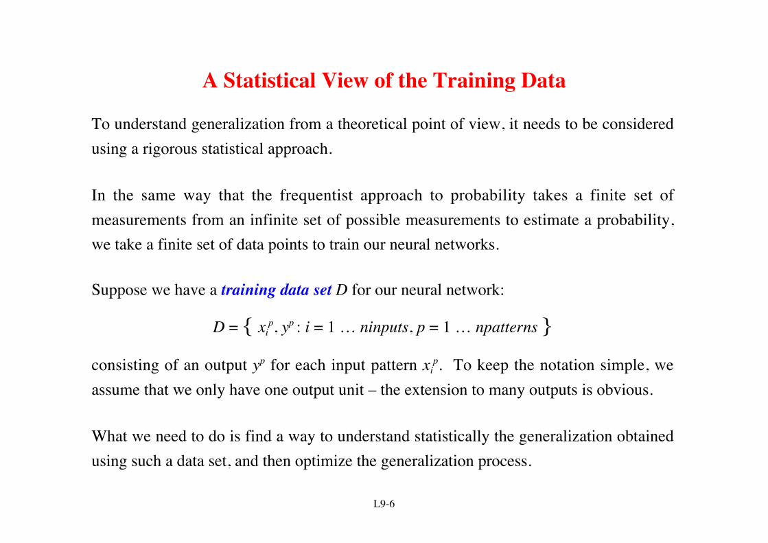
To understand generalization from a theoretical point of view, it needs to be consideredusing a rigorous statistical approach.

In the same way that the frequentist approach to probability takes a finite set ofmeasurements from an infinite set of possible measurements to estimate a probability,we take a finite set of data points to train our neural networks.

Suppose we have a training data set D for our neural network:

D = { xip, yp : i = 1 … ninputs, p = 1 … npatterns }

consisting of an output yp for each input pattern xip. To keep the notation simple, we

assume that we only have one output unit – the extension to many outputs is obvious.

What we need to do is find a way to understand statistically the generalization obtainedusing such a data set, and then optimize the generalization process.

L9-7

A Regressive Model of the Data

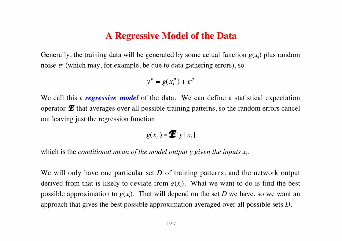
Generally, the training data will be generated by some actual function g(xi) plus randomnoise εp (which may, for example, be due to data gathering errors), so

yp = g(xip ) + ε p

We call this a regressive model of the data. We can define a statistical expectationoperator E that averages over all possible training patterns, so the random errors cancelout leaving just the regression function

€

g(xi ) =E [y | xi ]

which is the conditional mean of the model output y given the inputs xi.

We will only have one particular set D of training patterns, and the network outputderived from that is likely to deviate from g(xi). What we want to do is find the bestpossible approximation to g(xi). That will depend on the set D we have, so we want anapproach that gives the best possible approximation averaged over all possible sets D.

L9-8

A Statistical View of Network Training

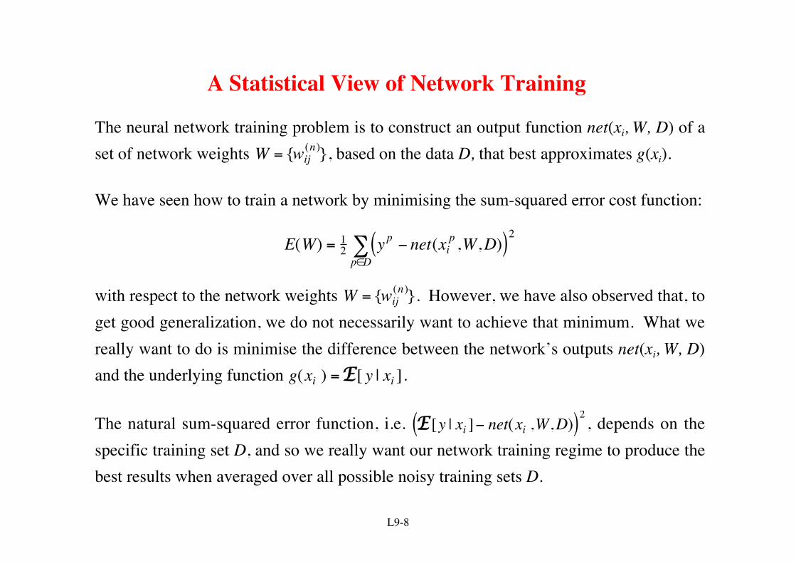
The neural network training problem is to construct an output function net(xi, W, D) of aset of network weights W = {wij

(n)}, based on the data D, that best approximates g(xi).

We have seen how to train a network by minimising the sum-squared error cost function:

E(W) = 12 yp − net(xi

p ,W,D)( )2p∈D∑

with respect to the network weights W = {wij(n)}. However, we have also observed that, to

get good generalization, we do not necessarily want to achieve that minimum. What wereally want to do is minimise the difference between the network’s outputs net(xi, W, D)and the underlying function g(xi ) =E[ y | xi ].

The natural sum-squared error function, i.e. E [y | xi ]− net(xi ,W,D)( )2 , depends on thespecific training set D, and so we really want our network training regime to produce thebest results when averaged over all possible noisy training sets D.

L9-9

Computing the Expected Generalization Error

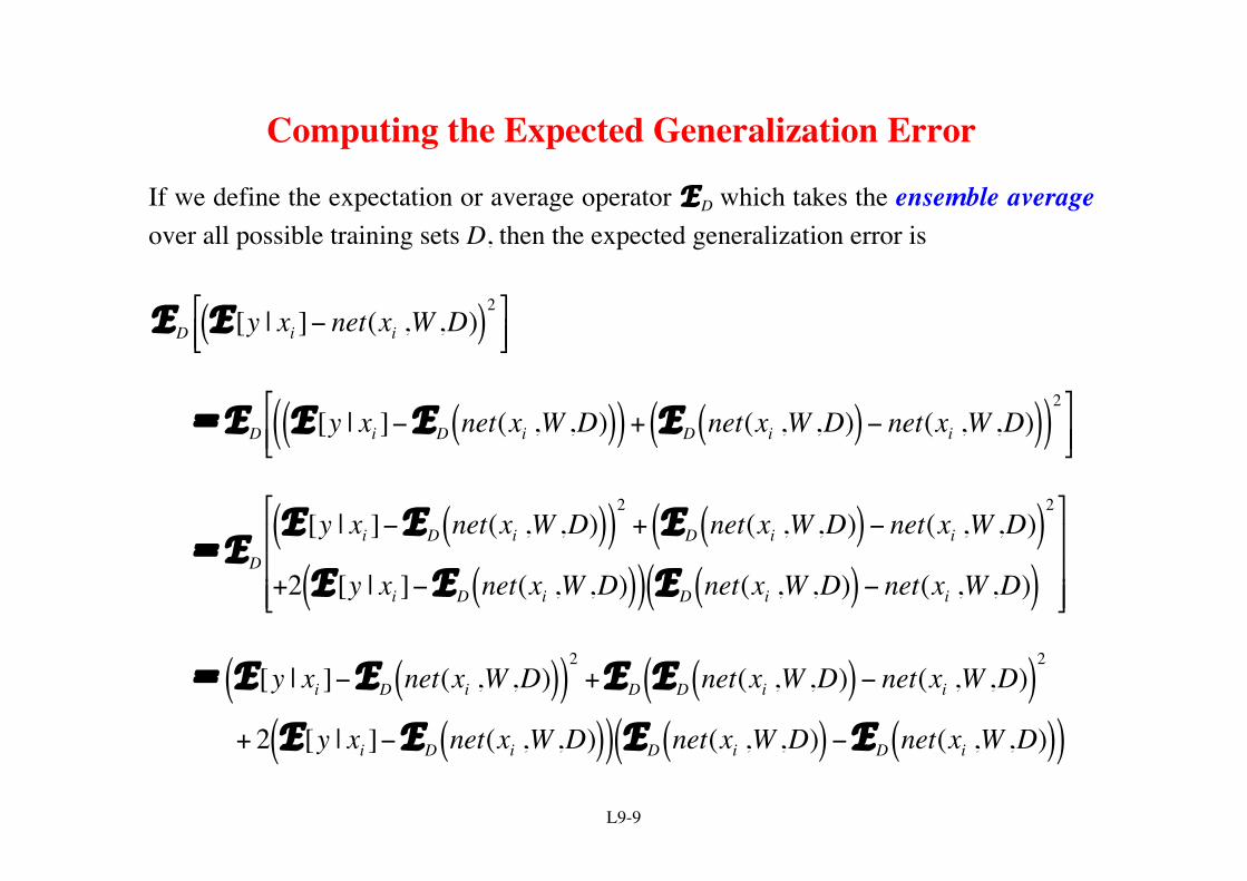
If we define the expectation or average operator ED which takes the ensemble averageover all possible training sets D, then the expected generalization error is

€

ED E [y | xi ]− net(xi ,W ,D)( )2

€

= ED E [y | xi ]−ED net(xi ,W ,D)( )( ) + ED net(xi ,W ,D)( )− net(xi ,W ,D)( )( )2

€

= ED

E [y | xi ]−ED net(xi ,W ,D)( )( )2

+ ED net(xi ,W ,D)( )− net(xi ,W ,D)( )2

+2 E [y | xi ]−ED net(xi ,W ,D)( )( ) ED net(xi ,W ,D)( )− net(xi ,W ,D)( )

€

= E[y | xi ]−ED net(xi ,W ,D)( )( )2

+ED ED net(xi ,W ,D)( )− net(xi ,W ,D)( )2

+ 2 E[y | xi ]−ED net(xi ,W ,D)( )( ) ED net(xi ,W ,D)( )−ED net(xi ,W ,D)( )( )

L9-10

Bias and Variance

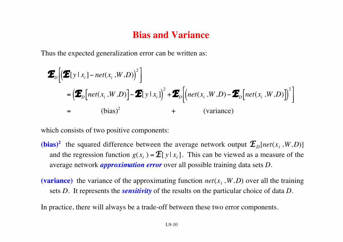
Thus the expected generalization error can be written as:

€

ED E [y | xi ]− net(xi ,W ,D)( )2

= ED net(xi ,W ,D)[ ]−E[y | xi ]( )2

+ED net(xi ,W ,D)−ED net(xi ,W ,D)[ ]( )2

= (bias)2 + (variance)

which consists of two positive components:

(bias)2 the squared difference between the average network output ED[net(xi ,W,D)]and the regression function g(xi ) =E[ y | xi ]. This can be viewed as a measure of theaverage network approximation error over all possible training data sets D.

(variance) the variance of the approximating function net(xi ,W,D) over all the trainingsets D. It represents the sensitivity of the results on the particular choice of data D.

In practice, there will always be a trade-off between these two error components.

L9-11

Extreme Case of Bias and Variance – Under-fitting

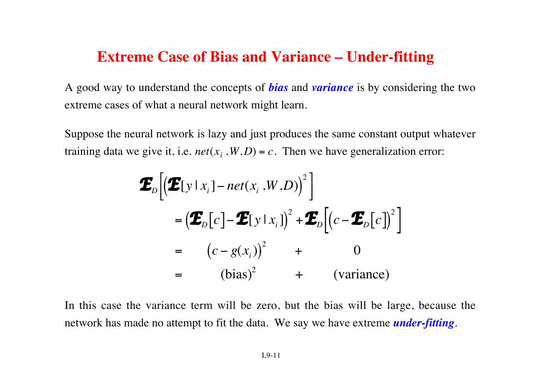
A good way to understand the concepts of bias and variance is by considering the twoextreme cases of what a neural network might learn.

Suppose the neural network is lazy and just produces the same constant output whatevertraining data we give it, i.e. net(xi ,W,D) = c. Then we have generalization error:

€

ED E [y | xi ]− net(xi ,W ,D)( )2

= ED c[ ]−E[y | xi ]( )2+ED c−ED c[ ]( )2[ ]

= c− g(xi )( )2 + 0

= (bias)2 + (variance)

In this case the variance term will be zero, but the bias will be large, because thenetwork has made no attempt to fit the data. We say we have extreme under-fitting.

L9-12

Extreme Case of Bias and Variance – Over-fitting

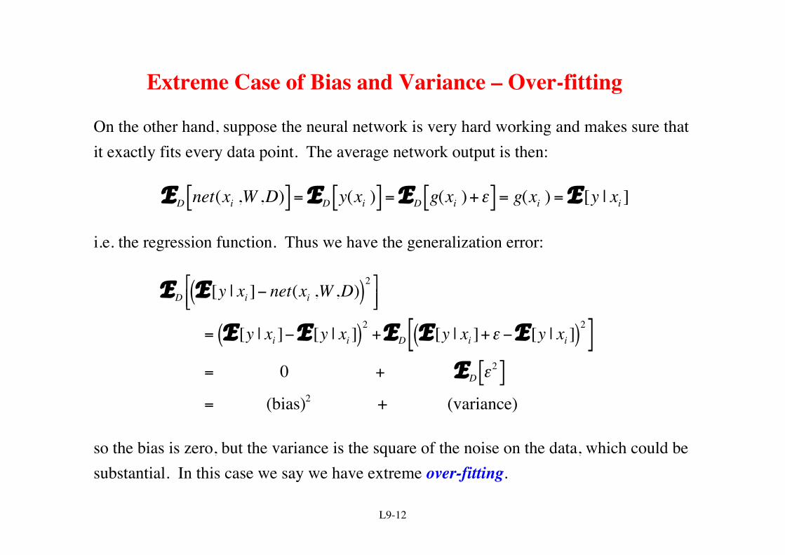
On the other hand, suppose the neural network is very hard working and makes sure thatit exactly fits every data point. The average network output is then:

€

ED net(xi ,W ,D)[ ] =ED y(xi )[ ] =ED g(xi )+ε[ ] = g(xi ) =E [y | xi ]

i.e. the regression function. Thus we have the generalization error:

€

ED E [y | xi ]− net(xi ,W ,D)( )2

= E [y | xi ]−E [y | xi ]( )2+ED E [y | xi ]+ε −E [y | xi ]( )2[ ]

= 0 + ED ε2[ ]

= (bias)2 + (variance)

so the bias is zero, but the variance is the square of the noise on the data, which could besubstantial. In this case we say we have extreme over-fitting.

L9-13

Examples of the Two Extreme Cases

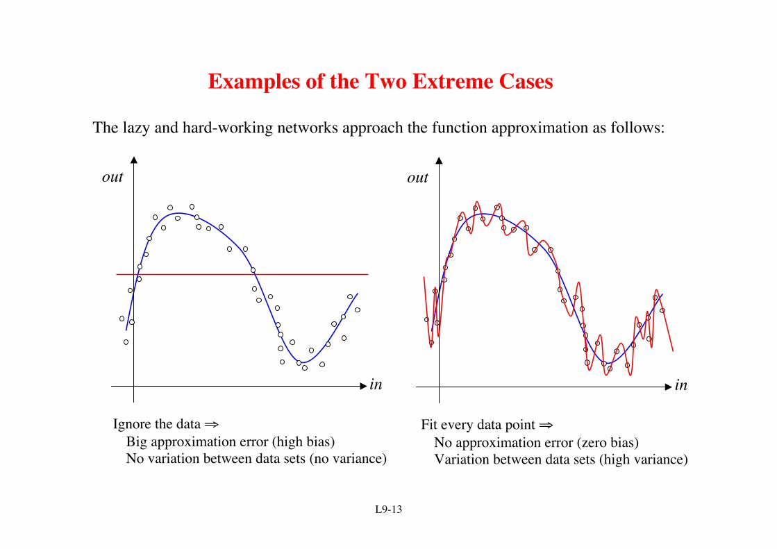
The lazy and hard-working networks approach the function approximation as follows:

Ignore the data ⇒Big approximation error (high bias)No variation between data sets (no variance)

Fit every data point ⇒No approximation error (zero bias)Variation between data sets (high variance)

out

in

out

in

L9-14

The Bias/Variance Trade-off

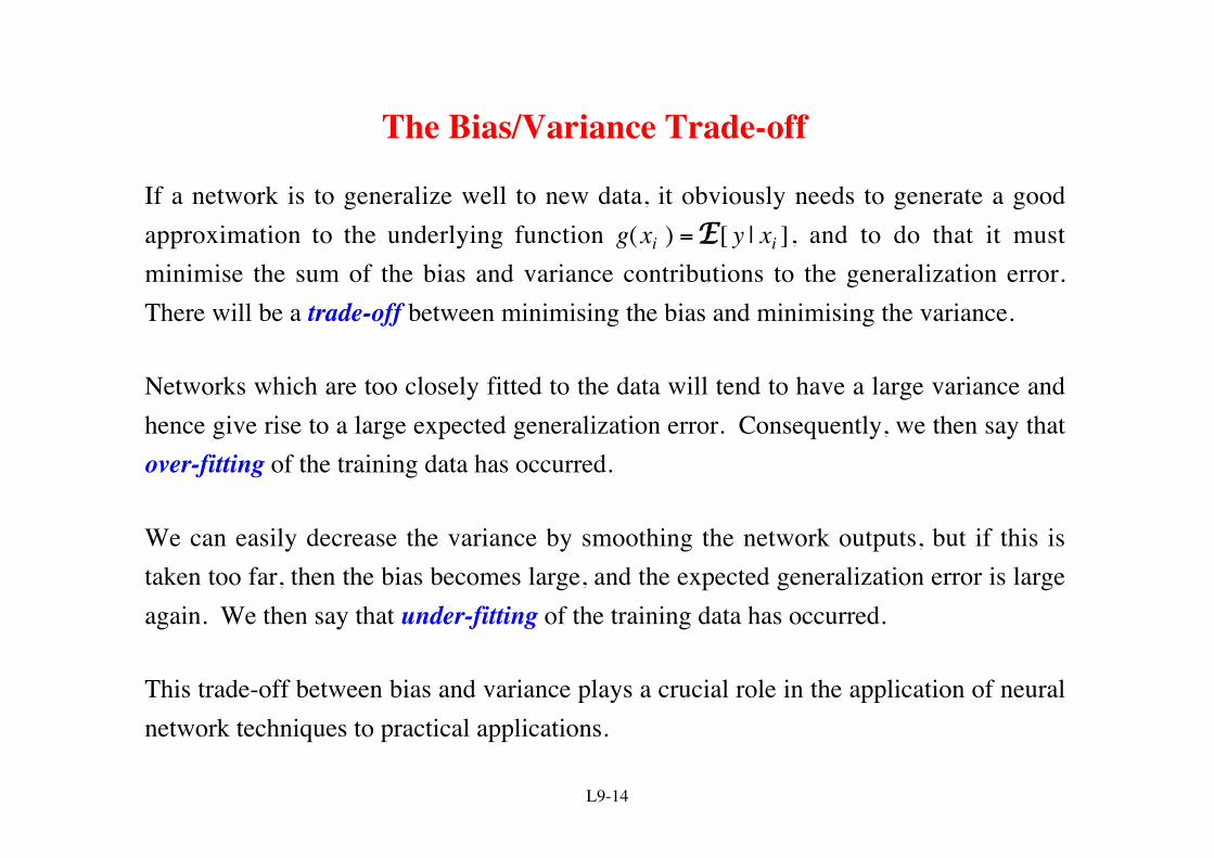
If a network is to generalize well to new data, it obviously needs to generate a goodapproximation to the underlying function g(xi ) =E[ y | xi ], and to do that it mustminimise the sum of the bias and variance contributions to the generalization error.There will be a trade-off between minimising the bias and minimising the variance.

Networks which are too closely fitted to the data will tend to have a large variance andhence give rise to a large expected generalization error. Consequently, we then say thatover-fitting of the training data has occurred.

We can easily decrease the variance by smoothing the network outputs, but if this istaken too far, then the bias becomes large, and the expected generalization error is largeagain. We then say that under-fitting of the training data has occurred.

This trade-off between bias and variance plays a crucial role in the application of neuralnetwork techniques to practical applications.

L9-15

Preventing Under-fitting and Over-fitting

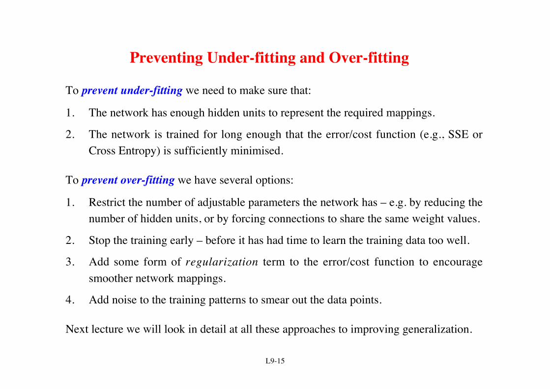
To prevent under-fitting we need to make sure that:

1. The network has enough hidden units to represent the required mappings.

2. The network is trained for long enough that the error/cost function (e.g., SSE orCross Entropy) is sufficiently minimised.

To prevent over-fitting we have several options:

1. Restrict the number of adjustable parameters the network has – e.g. by reducing thenumber of hidden units, or by forcing connections to share the same weight values.

2. Stop the training early – before it has had time to learn the training data too well.

3. Add some form of regularization term to the error/cost function to encouragesmoother network mappings.

4. Add noise to the training patterns to smear out the data points.

Next lecture we will look in detail at all these approaches to improving generalization.

L9-16

Overview and Reading

1. We began by looking at the computational power of MLPs.

2. Then we saw why the generalization is often better if we don’t train thenetwork all the way to the minimum of its error function.

3. A statistical treatment of learning showed that there was a trade-offbetween bias and variance.

4. Both under-fitting (resulting in high bias) and over-fitting (resulting inhigh variance) will result in poor generalization.

5. There are many ways we can try to improve generalization.

Reading

1. Bishop: Sections 6.1, 9.12. Haykin-2009: Sections 2.7, 4.11, 4.123. Gurney: Sections 6.8, 6.9