bh tomo – A Matlab borehole georadar 2D and 3D tomography

bh tomo – A Matlab borehole georadar 2D and3D tomography package

Bernard GirouxYiping Han

User’s guide

Preliminary version

Institut national de la recherche scientifiqueJuly 11, 2014

Contents

1 Introduction 7

2 Georadar tomography 92.1 General principles . . . . . . . . . . . . . . . . . . . . . . . . . . . . . . . . . . . . 92.2 Implementations . . . . . . . . . . . . . . . . . . . . . . . . . . . . . . . . . . . . 12

2.2.1 least-squares approach . . . . . . . . . . . . . . . . . . . . . . . . . . . . . 122.2.2 Geostatistical inversion . . . . . . . . . . . . . . . . . . . . . . . . . . . . 13

2.3 Ray tracing . . . . . . . . . . . . . . . . . . . . . . . . . . . . . . . . . . . . . . . . 162.3.1 Discretization of the slowness model . . . . . . . . . . . . . . . . . . . . . 162.3.2 Implementation . . . . . . . . . . . . . . . . . . . . . . . . . . . . . . . . . 18

3 Software package description 213.1 Main user’s interface . . . . . . . . . . . . . . . . . . . . . . . . . . . . . . . . . . 21

3.1.1 General processing flow . . . . . . . . . . . . . . . . . . . . . . . . . . . . 213.2 Database management . . . . . . . . . . . . . . . . . . . . . . . . . . . . . . . . . 22

3.2.1 Boreholes . . . . . . . . . . . . . . . . . . . . . . . . . . . . . . . . . . . . 233.2.2 Multi-offset gathers . . . . . . . . . . . . . . . . . . . . . . . . . . . . . . . 243.2.3 Panels . . . . . . . . . . . . . . . . . . . . . . . . . . . . . . . . . . . . . . 323.2.4 General processing flow . . . . . . . . . . . . . . . . . . . . . . . . . . . . 32

3.3 Traveltime processing . . . . . . . . . . . . . . . . . . . . . . . . . . . . . . . . . 343.3.1 Manual picking . . . . . . . . . . . . . . . . . . . . . . . . . . . . . . . . . 343.3.2 Semi-automatic picking . . . . . . . . . . . . . . . . . . . . . . . . . . . . 353.3.3 Automatic picking . . . . . . . . . . . . . . . . . . . . . . . . . . . . . . . 39

3.4 Amplitudes processing . . . . . . . . . . . . . . . . . . . . . . . . . . . . . . . . . 393.5 Fitting the model covariance . . . . . . . . . . . . . . . . . . . . . . . . . . . . . . 403.6 Inversion . . . . . . . . . . . . . . . . . . . . . . . . . . . . . . . . . . . . . . . . . 413.7 Estimating the saturation of the magnetic nanofluid . . . . . . . . . . . . . . . . 43

3.7.1 Background . . . . . . . . . . . . . . . . . . . . . . . . . . . . . . . . . . . 433.7.2 User interface . . . . . . . . . . . . . . . . . . . . . . . . . . . . . . . . . . 46

4 Example 49

A Exchange files formats 55A.1 Aramco’s Magnetic NanoMappers data . . . . . . . . . . . . . . . . . . . . . . . 55

A.1.1 Motivation for the format . . . . . . . . . . . . . . . . . . . . . . . . . . . 55

3

4 CONTENTS

A.2 Picked arrival times . . . . . . . . . . . . . . . . . . . . . . . . . . . . . . . . . . . 57A.3 Model constraints . . . . . . . . . . . . . . . . . . . . . . . . . . . . . . . . . . . . 57A.4 Inversion results . . . . . . . . . . . . . . . . . . . . . . . . . . . . . . . . . . . . . 58

B LSQR inversion parameters 59

List of Figures

2.1 Illustration of domain discretization . . . . . . . . . . . . . . . . . . . . . . . . . 102.2 Different graph templates allowing for different angular coverage . . . . . . . . 172.3 Illustration of elementary cells with location of primary and secondary nodes. . 18

3.1 Interactive screen of bh tomo. . . . . . . . . . . . . . . . . . . . . . . . . . . . . . 223.2 Interactive screen of bh tomo db. . . . . . . . . . . . . . . . . . . . . . . . . . . . 233.3 Add borehole. . . . . . . . . . . . . . . . . . . . . . . . . . . . . . . . . . . . . . . 233.4 Definitions of borehole coordinates. . . . . . . . . . . . . . . . . . . . . . . . . . 243.5 3D view of the boreholes. . . . . . . . . . . . . . . . . . . . . . . . . . . . . . . . 253.6 Borehole survey modes . . . . . . . . . . . . . . . . . . . . . . . . . . . . . . . . . 253.7 Convention for transmitter (Tx) and receiver (Rx) coordinates. . . . . . . . . . . 263.8 Illustration of the two ways to input increasing distances between Tx and Rx

antennas for air shots. . . . . . . . . . . . . . . . . . . . . . . . . . . . . . . . . . 273.9 Import MOG dialog window. . . . . . . . . . . . . . . . . . . . . . . . . . . . . . 273.10 Window showing raw MOG data. . . . . . . . . . . . . . . . . . . . . . . . . . . 283.11 Zero-offset profile display window. . . . . . . . . . . . . . . . . . . . . . . . . . . 283.12 Example of air shot data and statistics on picked traveltimes. . . . . . . . . . . . 293.13 PSD estimates window . . . . . . . . . . . . . . . . . . . . . . . . . . . . . . . . . 303.14 Ray coverage for a MOG dataset. . . . . . . . . . . . . . . . . . . . . . . . . . . . 313.15 Utility window to prune MOG datasets. . . . . . . . . . . . . . . . . . . . . . . . 313.16 Illustration of reference point and feed point of dipole antennas. . . . . . . . . . 323.17 Interactive screen of bh tomo grille. . . . . . . . . . . . . . . . . . . . . . . . 333.18 Interactive screen of bh tomo tt. . . . . . . . . . . . . . . . . . . . . . . . . . . . 343.19 Example of first-cycle isolation. The original trace, in blue, has a dominant fre-

quency of 177 MHz. This trace is crosscorrelated with a 177 MHz syntheticwavelet, shown in red. After the application of the time window, the scatteredarrivals are eliminated, as shown in green. . . . . . . . . . . . . . . . . . . . . . . 36

3.20 Illustration of the effect of time rescaling for three synthetic traces having differ-ent dominant frequencies. The traces are aligned without (left) and with (right)time rescaling. . . . . . . . . . . . . . . . . . . . . . . . . . . . . . . . . . . . . . . 37

3.21 Interactive screen of bh tomo pick. . . . . . . . . . . . . . . . . . . . . . . . . . 383.22 Interactive screen of bh tomo amp. . . . . . . . . . . . . . . . . . . . . . . . . . . 403.23 Interactive screen of bh tomo fitCovar. . . . . . . . . . . . . . . . . . . . . . . 41

5

6 LIST OF FIGURES

3.24 Interactive screen of bh tomo inv. Two velocity models obtained with the datapresented in section 4 are displayed. The leftmost model is obtained by cokrig-ing and the rightmost model is the simulation that best fits the data. . . . . . . . 42

3.25 Accuracy of the saturation estimates with exact input parameters. . . . . . . . . 463.26 Accuracy of the saturation estimates for inaccurate velocity and attenuation in-

put data. . . . . . . . . . . . . . . . . . . . . . . . . . . . . . . . . . . . . . . . . . 47

4.1 Schematic cross-section of the surveyed structure interpreted from boring logs. 504.2 Ray coverage for the velocity model shown in Fig. 3.24. Grayed out rays were

excluded for attenuation tomography. . . . . . . . . . . . . . . . . . . . . . . . . 514.3 Simulation results of the geostatistical inversion of amplitude data, amplitude

ratio method. On the left: simulation that best fits the data. On the right: stan-dard deviation infered from the 128 simulations. . . . . . . . . . . . . . . . . . . 52

4.4 Simulation results of the geostatistical inversion of amplitude data, centroid fre-quency down-shift method. On the left: simulation that best fits the data. Onthe right: standard deviation infered from the 128 simulations. . . . . . . . . . . 53

4.5 Maps of dielectric constant and effective electric conductivity infered from thetomographic results. Boreholes 1, 2 and 3 are drawn in green. . . . . . . . . . . 54

Chapter 1Introduction

In the last two decades, borehole georadar has received increasing attention for mineral explo-ration as well as for hydrogeological and geotechnical studies (Olsson et al., 1992; Hubbardet al., 1997; Giroux et al., 2004; Tronicke et al., 2004). Information about the electromagneticvelocity and attenuation structures can be obtained from the inversion of cross hole georadartravel times and amplitudes, respectively. Combined inversions of georadar travel times andamplitudes may thus allow to separate the effects of dielectric permittivity and electric con-ductivity on electromagnetic wave propagation (Zhou and Fullagar, 2001). Therefore, to invertfor both velocity and attenuation greatly enhance the understanding of the probed media.

Besides, unless straight rays are used, attenuation tomography requires that raypaths beknown to render possible the integration of the unknown parameter along the wave trajectory.Therefore, velocity tomography must be performed prior to the inversion of the amplitudedata. Once the velocity field is known, ray tracing allows to infer the curved raypaths associ-ated to each measured travel time and amplitude. In fact, inversion of the travel times is nonlinear and is solved iteratively by updating the raypaths at each iteration. When the data toinvert was acquired in many boreholes and in different configurations (cross-hole or verticalradar profiling), it becomes somewhat cumbersome to keep the travel time, amplitude andraypath data sets consistent. A motivation for the development of bh tomo was to facilitatethe management of these data.

Another important motivation for the development of the bh tomo package is to make animplementation of the geostatistical inversion scheme of Gloaguen et al. (2005) available. Thismethod offers many advantages over least-squares based algorithms. The main advantages ofthe new method are that it is self-regularized and requires less a priori information, it allows theidentification of stable characteristics and uncertain features through stochastic simulations,and it allows the exact fitting of any linear constraints on the sought parameter. Also, thecovariance model of the unknown field is determined by the method. This implies that theapproach can be advantageous in applications where stochastic simulations are used withouta priori information about the spatial properties of the studied parameters.

The Matlab programming environment, commercialized by The MathWorks, was selectedfor the development of bh tomo for several reasons, namely because it combines extensivenumeric computation libraries, a higher-level programming language as well as visualizationcapabilities and easy GUI development tools. Matlab has been used widely for geophysicalapplications (e.g. Beaty et al., 2002; Conroy and Radzevicius, 2003; Rucker and Ferre, 2004;Witten, 2002). In addition, Matlab programs are portable across platforms supported by The

7

8 1 Introduction

MathWorks (Mac OS X, UNIX/Linux, Windows). bh tomo has been developed as free soft-ware with a GNU license, allowing public access to the source code. The package may beused for any purpose including educational, research and commercial applications. Users areencouraged to modify and add to the existing package to suit their specific needs.

The main features of the package are:

• Ray-based approach

– Travel time tomography;– Attenuation tomography based on first-cycle amplitude.

• Two types of ray-tracing routines

– Straight rays in homogeneous velocity models;– Curved rays in heterogeneous models.

• Two-dimensional domains:

– Arbitrary position of transmitters & receiver in the 2D plane (arbitrary well trajec-tory).

• Three-dimensional domains.

• Various data input format:

– RAMAC (Mala Geosciences);– PulseEKKO (Sensors & Software);– SEGY.

• Handle of time units and tomography on seismic data as well

• Two core inversion options:

– Classic least-squares solver;– Geostatistical tomography and simulation.

• Elliptical anisotropy (with geostatistical approach) for 2D domains.

• Treatment of time-lapse data.

• Basic database functionality with graphical user interface.

• 2D and 3D visualisations.

• Basic interpretation module

• Released under the GNU General Public License, version 3.

The software package relies on a mini database and comprises interactive modules to manage,process and interpret the data. This user’s guide is organised by module, but a first chapterabout tomography is presented.

Chapter 2Georadar tomography

2.1 General principles

Tomographic georadar measurements are accomplished by using a transmitting antenna (Tx)located in a borehole to emit a high frequency electromagnetic pulse. The radiated pulse prop-agates within the medium with velocity v, and is eventually recorded at a receiving antenna(Rx) located in another hole a known distance away. The recording, refered to as a trace, is thevoltage at the receiver as a function of time. Hence, the trace contains the transmitted waveletarriving at time t, as well as other waves produced by eventual reflections or refractions of theemitted pulse. One approach to tomographic inversion is to retrieve the arrival time of the di-rect wave and use it to obtain the velocity between the transmitter and receiver by consideringthat the wave traveled along a raypath. Another approach is to consider all the informationcontained in the trace, i.e. the whole waveform, to reconstruct the physical properties distribu-tions between the transmitter and receiver (Cai et al., 1996; Ernst et al., 2007). Waveform-basedalgorithms require extensive computational resources. Hence, in the development of bh tomoonly the former has been considered so far, i.e. the ray-based approach.

Following the theory of geometrical optics, to each transmitted wavelet can be associateda raypath l, which is a curve describing the trajectory of the wave between the Tx and Rxantennas. The travel time is related to the slowness s, i.e. the reciprocal of velocity, and raypathby

t =Z

rays(l) dl. (2.1)

During a survey, the recording process is repeated for various Tx and Rx positions along theholes, in order to have the raypaths cover the whole area between the two holes. After comple-tion of the survey, the arrival times of the direct waves are picked from each trace, and thesedata are used to perform the travel time tomography calculations. For no traces, this datatakes the form of a no ⇥ 1 matrix called t. The aim of the tomography is to obtain the velocityfield, or its inverse the slowness, between the two boreholes. To perform the calculations, theslowness field must be discretized into np cells, yielding a matrix s containing the np ⇥ 1 un-known slownesses. This discretization implies that the raypaths are split into segments (seeFig. 2.1). Each segment has a length equal to the distance the ray travels in that cell. The traveltime associated with a raypath becomes the sum of each segment times the slowness of the

9

10 2 Georadar tomography

S2S1 S3 S4 S5

S6 S7 S8

S9

S10

S11 S12 S13 S14 S15

S16

S17

S18 S19 S20

S21 S22 S23 S24 S25

i17

i13

i8

i4i5

l

i16l

l

l

i9l

ll

li12

Tx

Rx

Figure 2.1: Illustration of domain discretization and consecutive raypath segmentation. Eachsegment has a length equal to the distance the ray travels in the cells it is traversing. The traveltime is the sum of each segment times the slowness of the corresponding cell.

corresponding cell:

t =segments

Âi=1

sili. (2.2)

Gathering all measured travel times in vector d and unknown slownesses in vector m, a sys-tem of equations of the form

Gm = d (2.3)

can be built, with G being a sparse no ⇥ np matrix. The objective of the tomographic calcu-lation is to solve this system for the slowness vector m. Note that the problem is nonlinearbecause, by virtue of Fermat’s principle, the raypaths are function of the slowness field. Fer-mat’s principle states that the path of a ray between two points is the path that minimizes thetravel time. Consequently, rays tend to “bend around” low velocity zones and “concentrate”in high velocity zones. This nonlinearity implies that the tomographic problem must be solvediteratively.

So far the focus has been on travel time tomography. Often, e.g. in environmental and hy-drogeological applications, it is interesting to know the dielectric constant k within the probedmedium, because it is related to the volumetric water content (by definition k = ee/e0 wheree0 is the dielectric permittivity of free space)1. Usually, it is common practice to perform traveltime tomography alone to compute the dielectric constant k. This approach is valid when elec-trical loss is low, i.e. when the condition se

wee⌧ 1 is satisfied. Here, w is the angular frequency

equal to 2p f , f being the frequency of the radio wave, se is the effective electrical conductivityand ee is the effective dielectric permittivity (for a discussion on effective parameters, see e.g.Turner and Siggins (1994)). Under the low loss condition, the velocity is

v =1p

µee. (2.4)

Note that most earth materials are non magnetic, and in general their magnetic permeabilitycan be assumed to be equal to the permeability of free space µ0. Therefore, the dielectric

1Several empirical and theoretical models exist that relate k to the volumetric water content. See Huisman et al.(2003) and Sihvola (2000) for reviews.

2.1 General principles 11

constant is obtained fromk =

1v2µ0e0

. (2.5)

However, the above expression yields inaccurate results in media with high electric loss, i.e. ifthe electrical conductivity se is close to, or higher than, the product of permittivity ee and w(Giroux and Chouteau, 2010). In such circumstances, the dielectric constant must be evaluatedfrom both the velocity and attenuation. With the attenuation a in Np/m, the dielectric constantis

k =1

µ0e0

1v2 �

⇣ a

w

⌘2�

. (2.6)

Although not rigorously extact in the context of a ray-based framework, Eq. (2.6) yields a morerepresentative estimate of k than Eq. (2.5). As mentioned in introduction, another reason toinvert for attenuation is that its knowledge allows to infer the electrical conductivity structureand leads to an increased comprehension of the probed medium. The value of the effectiveconductivity is

se =2a

µ0v. (2.7)

Various methods exist to compute the attenuation within the medium. In bh tomo, twomethods are implemented: the amplitude ratio (Olsson et al., 1992) and the centroid frequencydown shift method (Quan and Harris, 1997; Liu et al., 1998). In the former, the attenuation isobtained from the ratio of the emitted amplitude to the received amplitude. In this method,the received amplitude must be processed so that it can be linearly related to the attenuation.In short, the amplitude measured at the receiver Am is an exponential decay of the initialamplitude at the source A0, times a correction term taking into account the radiation patternsof the antennas (QTx and QRx) and the geometrical spreading of the wave:

Am = A0 exp✓�

Z

raya(l) dl

◆QTxQRx

l. (2.8)

The terms A0, QTx and QRx cannot be easily known and in most cases are approximated. Thismakes amplitude tomography somewhat less robust than travel time tomography. Detailsand discussion on amplitude data reduction can be found in Peterson (2001) and Holligeret al. (2001). However, once A0, QTx and QRx are estimated, taking the natural logarithm ofEq. (2.8) leads to

t =Z

raya(l) dl, (2.9)

wheret = ln(A0) + ln(QTxQRx)� ln(Aml). (2.10)

Equation (2.9) has the same form as Eq. (2.1). This means that the algorithms developed tosolve Eq. (2.1) are applicable for Eq. (2.9).

Let us now consider the estimation of the attenuation from the frequency content of thedata. Quan and Harris (1997) introduced the concepts and applied them for seismic tomogra-phy, and Liu et al. (1998) applied the method to GPR data. The technique is based on linearsystem theory which is used to describe the propagation of the EM wave in the ground. In suchcase, the amplitude spectrum at the receiver R( f ) is the product of the instrument/mediumresponses G( f )H( f ) with the amplitude spectrum of the incident wave S( f ), i.e. R( f ) =


G( f )H( f )S( f ). The term G( f ) includes the instrument response, geometrical spreading, source-receiver coupling, radiation patterns, reflection/transmission coefficients and the phase accu-mulation caused by propagation; and H( f ) is the attenuation filter describing the variation ofamplitude due to absorption in the probed medium. The attenuation filter has the form

H( f ) = exp✓� f

Z r

0a0 ds

◆, (2.11)

where a0 = a/ f . The goal is to get an estimate for this parameter. The main assumption of thetechnique is that G must be independent of frequency. When this is the case, the integral of a0can be obtained directly from the logarithm of the ratio S( f )/R( f ). However, there are twodifficulties to this procedure, the first being that S( f ) is generally unknown, and the secondbeing that calculations based on individual frequencies are subject to instabilities due to poorsignal-to-noise ratio. This is the reason why Quan and Harris (1997) introduced the centroidfrequency, defined for a given signal X( f ) as

fX =

R •0 f X( f )d fR •

0 X( f )d f, (2.12)

with the variance being

s2X =

R •0 ( f � fX)2X( f )d f

R •0 X( f )d f

. (2.13)

They showed that the difference between the source and receiver centroid frequencies, fS andfR respectively, are related to the integral of the attenuation by

fS � fR = B2Z r

0a0 ds, (2.14)

where B2 takes into account the type of source spectrum and variance of the centroid fre-quency. For Gaussian spectrum, B2 is equal to the variance s2

S . One problem with equa-tion (2.14) is that both a0 and fS are unknown. In bh tomo, fS is found by linear regressionand can also be manually edited. Also, by virtue of linear system theory, s2

S and s2R are equal.

s2S is therefore estimated from the values of s2

R computed from the radargrams. Once fS and s2S

are deduced, we obtain, in discrete form for the ith trace and for a Gaussian source spectrum:

ti =N

Âj

ajlij, (2.15)

where in this case ti = f ( fS � f iR)/s2

S . This linear system can be solved by using the samealgorithm than the one developed for velocity analysis.

2.2 Implementations

2.2.1 least-squares approach

Until recently, variants of least-squares algorithms were almost the exclusive approach to solv-ing the tomographic problem, which reduces to solving the system

Gm = d (2.16)

2.2 Implementations 13

where in our case G represents a no ⇥ np matrix including the partial derivatives (ray seg-ment lengths), m the np slowness or attenuation values and d the no travel time or amplitudedata. Because this problem is inherently ill-posed, least-squares algorithms rely on so-calledregularization techniques to stabilize the solution.

The least-squares approach implemented in bh tomo is regularized using a smoothnessconstraint, i.e. the objective function to minimize has the form

kGm� dk2 + lkDmk2, (2.17)

where D is the second order spatial derivative matrix and l is a Lagrange multiplier (Menke,1989). The LSQR algorithm of Paige and Saunders (1982) has proved very effective to solvethis type of system (Nolet, 1993). This algorithm can handle unsymmetric equations, and it istherefore possible to avoid the computation of the transpose matrices of G and D required inthe classic least-squares solution. This property is used in bh tomo, in which the system

G

lD

�m =

d0

�, (2.18)

is fed to a slightly modified version of the lsqr.m routine available at http://www.stanford.edu/group/SOL/software/lsqr.html.

Another constraint can be added to the system through the imposition of model param-eter values at given locations. For a vector mc containing nc of these values, this is done byincorporating a nc ⇥ np matrix M to the system, such that

2

4G

lDM

3

5 m =

2

4d0

mc

3

5 . (2.19)

For each line of the matrix M, all values are equal to zero except for the column correspond-ing to the model cell where the parameter is known. For example, if the values are to beconstrained only the first and last cells, M and mc will be respectively

1 0 · · · 0 00 0 · · · 0 1

�and

mc1mcnp

�. (2.20)

The advantage of this approach is that the LSQR algorithm can still be used to solve the system.On the other hand, the values of mc will never be exactly fitted due to the averaging effectimposed by the smoothness criteria.

2.2.2 Geostatistical inversion

Very often, the results of regularized least-squares algorithms are sensitive to the values ofregularization Lagrange multipliers, which cannot easily be adjusted automatically. To cir-cumvent this problem, an approach based on geostatistical analysis of the travel time data hasbeen developed by Gloaguen et al. (2005). As reviewed below, it can be shown that the covari-ance model of the slowness field can be modeled from the travel time data. This covariancemodel describes the spatial characteristics of the slowness field. Using this covariance modeland the fact that slowness and travel time are linearly related, it is possible to cokrig the slow-ness field using the travel time data. Cokriging is an interpolation technique allowing to usea more intensely sampled covariate (the travel time) in the estimation of values for a related

http://www.stanford.edu/group/SOL/software/lsqr.html

http://www.stanford.edu/group/SOL/software/lsqr.html


variate (the slowness) (Chiles and Delfiner, 1999). The procedure is said to be self-regularizedbecause regularization is supported entirely by the data. It is also easy to go further and toimpose slowness gradients or even any kind of linear constraint to the solution.

For known raypaths, slowness and travel time are linearly related. As a consequence, theircovariance matrices are also linearly related. To illustrate this, define first the error betweennoise-free data d and the measured data d⇤ as

e = d⇤ � d. (2.21)

In the following development, it is assumed that the error has zero mean and is uncorrelatedwith time, i.e. the expectation value E[e] = 0 and the covariance Cov(d, e) = 0. Working inmatrix notation and replacing d by Gm, we can write d⇤ = Gm + e. Working with contrasts,i.e. imposing E[m] = 0 and E[d] = 0, we get

E[d⇤] = E[Gm + e] = 0. (2.22)

Since d⇤ has zero mean, the observed data covariance matrix is simply

Cd⇤ = t⇤t⇤T. (2.23)

After manipulation, we get for the no ⇥ no data covariance matrix (Gloaguen et al., 2005)

Cd⇤ = GCmGT + C0 (2.24)

where Cm represents the np ⇥ np model parameter covariance matrix and C0 is the no ⇥ nodiagonal matrix of error variances or the nugget effect. Eq. 2.24 serves as the basis to ob-tain a model covariance function Cov(m, m) from the experimental data. Note that the co-variance Cov(d⇤, d⇤) is not stationary. Therefore, estimators such as traditional variogram orcovariogram cannot be used directly, and the model covariance function must be estimatedby inversion. The program bh tomo fitCovar, part of the package, is designed to accom-plish this task interactively using the concept of the V-V plot described in Asli et al. (2000),or automatically using a minimization scheme based on the Simplex method implementationof Matlab. The procedure is as following. Eq. (2.23) is first used to compute Cd

⇤. Then atheoretical covariance function Cov(m, m) is chosen for the model, as well as initial values ofrange, sill and a nugget effect. The matrix Cm is built for the tomographic inversion grid us-ing Cov(m, m), and the right term of Eq. (2.24) is finally computed. In the V-V plot approach,the so-called theoretical covariance values (right term of Eq. (2.24)) are sorted in decreasingorder and bined in classes for which the mean value is calculated. The same sorting order andbining scheme is applied to the experimental data Cd

⇤. Thus, a value corresponding roughlyto a single theoretical structural distance can be calculated for an experimental variogram. Ifthe chosen covariance function and parameters are appropriate, the experimental variogramversus theoretical variogram plot (the V-V plot) should show a dispersion around a line at 45�.The advantage of our approach is that the model covariance function parameters are tuned bythe observed data.

Once an acceptable model covariance function is obtained, the model parameter field iscokriged using the arrival times and any available known model data (Marcotte, 1991). Thisoperation requires the cross covariance Cov(d⇤, m) to be known. It can be shown from theprevious definitions that the cross covariance matrix is (Gloaguen et al., 2005)

Cdm = GCm. (2.25)

2.2 Implementations 15

In bh tomo, primal cokriging is implemented to estimate the model parameter field. Thecokriging weights are

L = (Cd⇤)�1 Cdm, (2.26)

and the cokriging estimator of the model parameter field is

Z⇤g = LTd⇤. (2.27)

An advantage of cokriging is that any known value of the model parameter that is introducedin the system of equation will be found in the solution. Suppose for example that mi modelparameter values are known with variance si at nc cells along the boreholes. The cokrigingweights become

L =

Cm

c CdmcT

Cdmc Cd

⇤

��1 Cm0

c

Cdm

�, (2.28)

where

Cmc =

2

6664

Cm11 Cm12 · · · Cm1nc

Cm21 Cm22 · · · Cm2nc...

... . . . ...Cmnc1 Cmnc2 · · · Cmncnc

3

7775+

2

6664

s1 0 · · · 00 s2 · · · 0...

... . . . ...0 0 · · · snc

3

7775, (2.29)

Cdmc =

2

6664

Cdm11 Cdm12 · · · Cdm1nc

Cdm21 Cdm22 · · · Cdm2nc...

... . . . ...Cdmno1 Cdmno2 · · · Cdmnonc

3

7775(2.30)

and

Cm0c =

2

6664

Cm11 Cm12 · · · Cm1np

Cm21 Cm22 · · · Cm2np...

... . . . ...Cmnc1 Cmnc2 · · · Cmncnp

3

7775. (2.31)

At this point, it is interesting to note the similarities between our approach, which in termsof Cd

⇤ and Cm is

Z⇤g =

2

64

0

@GCmGT + C0| {z }A

1

A�1

GCm| {z }B

3

75

T

d⇤, (2.32)

and the Bayesian formulation, which writes (Tarantola and Valette, 1982)

Dm = CmGT⇣

GCmGT + Cd

⌘�1Dd. (2.33)

The latter is usually transformed in the form (Nolet, 1993; Maurer et al., 1998)

Cd�1/2G

Cm�1/2

�m =

Cd�1/2(Dd + G)

c

�(2.34)

suitable in form to be solved using the LSQR algorithm. In the geostatistical framework, weuse a different approach because the matrix A in Eq. (2.32) is symmetric positive definite and


the system can be easily solved by Cholesky factorization. Apart from the differences in nu-merical solution of the above systems of equations, perhaps the most important advantage ofusing the geostatistical approach is that a model parameter covariance function constrainedby the measured data is obtained. As shown next, this allows to study the spatial variabilityof the model parameter and measure the robustness of the model.

By construction, cokriging gives a smooth estimate of the model parameter field. It may bedesirable and informative to obtain various reasonable solutions showing the kind of variabil-ity that can be expected from the model covariance function adopted. Within our framework,this can be done by using geostatistical simulation algorithms. Among the various simulationschemes, the FFT-MA algorithm (Le Ravalec et al., 2000) was retained for its rapidity. The FFT-MA algorithm generates non-conditional simulations Zs

g. Hence, the computed data of eachsimulation are not linked to the measured data. Therefore, it is necessary to post-condition thesimulation by cokriging to constrain the simulations. First, the cokriging of model parameterZ⇤g with measured data is performed using Eq. (2.27). Then, for each realization Zs

g, simulateddata are computed using the relationship ds = GZs

g + e, where e is drawn from a normaldistribution with zero mean and C0 variance. Keeping the same cokriging weights, cokrigingof the slowness Zs⇤

g with computed data ds is performed. Finally, the conditional simulatedmodel Zsc

g isZsc

g = Z⇤g + (Zsg � Zs⇤

g ). (2.35)

Zscg has the desired covariance and fits exactly any linear constraint on the model. When the

data covariances have zero nugget effect, the measured data and the computed data of eachconditional simulation are exactly the same. When a nugget effect is present on observed data,the computed data depart from the measured data by an amount compatible with the level oferror described by the nugget effect.

A measure of the robustness of the model can also be obtained by performing a large num-ber of simulations and storing each realization of the slowness field. The realizations are alldifferent and independent, but equally consistent with the measured data and the modeled co-variance. The probability that the slowness exceeds a given value can then be drawn from a setof N realizations as following. At a given point x in the model parameter map, the probabilityof m(x) being above a given threshold mt is

P(m(x) > mt) =1N

N

Âi=1

I(mi(x) > mt), (2.36)

with mi(x) being each realization i at point x and I(mi(x) > mt) the indicator taking value 1 ifmi(x) > mt and 0 otherwise.

2.3 Ray tracing

Raytring must be perfomed to build matrix G. In bh tomo, the shortest path method is used.The algorithm is described in the following.

2.3.1 Discretization of the slowness model

In the shortest path method, a grid of nodes is used to build a graph by connecting eachnode to its neighbours. The connections within the graph are assigned a length equal to thetraveltime along it. Hence, by virtue of Fermat’s principle which states that a seismic ray

2.3 Ray tracing 17

1st order 2nd order

3rd order

4th order

5th order

∆θ = 90° ∆θ = 45° ∆θmin = 18.4°

∆θmax = 26.6°

∆θmin = 7.1°

∆θmax = 18.4°

∆θmin = 3.2°

∆θmax = 14.0°

Figure 2.2: Different graph templates allowing for different angular coverage. For simplicity,only one quadrant of 2D templates are shown (after Matarese (1993)).

follows the minimum traveltime curve, the shortest path between two points within the graphcan be seen as an approximation of the raypath (Nakanishi and Yamaguchi, 1986).

Moser (1991) discusses briefly two ways of discretizing the slowness model: one attributedto Nakanishi and Yamaguchi (1986) in which grid nodes surround cells of constant slowness,and a second in which the slowness field is sampled at node locations. In the latter case,the sampling scheme may vary, but the nodes are generally distributed spatially in regularfashions such as on grids of cubic “cells”. Having nodes only at the corners of the cells limitsdrastically the allowed angular coverage, and various templates were designed to improvethis aspect. For example, high order templates can reach nodes many cells away from thesource point, as illustrated in Figure 2.2.

A drawback of using high order templates is that they require smooth slowness variationsto maintain accuracy, or dense node sampling in otherwise high contrast regions. Hence, thereis a trade-off to seek between accuracy and speed of computation. This is especially the casein inversion, where it is not always desirable to use very fine grids because this has for effectto increase the number of unknown in the system to solve, and therefore increase the overallcomputational effort. One could use two grids of different sizes, a coarser for the inversionstep and a finer for the raytracing step, and interpolate between the two, but this adds to thecomputational burden and causes additional inaccuracies. Besides, using high order templatescomplicates the problem of building a system of equation for the inverse problem becauseray segments will cross many cells and adequate bookkeeping increases the computationalburden. In this regard, a discretization scheme based on nodes surrounding cells of constantslowness as proposed by Nakanishi and Yamaguchi (1986) is appealing.

Gruber and Greenhalgh (1998) have proposed a variant of the discretization approach ofNakanishi and Yamaguchi (1986), which is well suited for the tomography problem and whichprovides adequate angular coverage. In their study on the accuracy of traveltime computationon 2D grids, they have used constant slowness cells with so-called primary nodes at the cornerof the cells in addition to so-called secondary nodes on the edges of the cells. Bai et al. (2007)have used the idea of primary and secondary nodes in 3D and incorporate nodes on the sidesof the cells. However, they interpolate the slowness at the secondary nodes and don’t useconstant slowness cells. In both cases, ray segments (or connections between two nodes) arecomprised within no more than one cell, which is very handy to simplify bookkeeping intomography applications.

In bh tomo, we follow Gruber and Greenhalgh (1998) and Bai et al. (2007) and use primary


Primary nodeSecondary node

(a) 2D cells

Primary nodes

Edge nodes

Side nodes } Secondary nodes

(b) 3D cell

Figure 2.3: Illustration of elementary cells with location of primary and secondary nodes.

and secondary nodes surrounding rectangular cells (in 2D) or cuboids (in 3D) at their cornersand on their edges and sides, as shown in Figure 2.3. The slowness value is assigned to thecell, not the nodes.

The raytracing algorithm retained in this work is synthesized in Algorithm 1, and proceedsas follows. After construction of the graph (i.e. establishing the allowed connections betweenthe nodes), all nodes are initialized to infinite time except the source node which is assignedits “time zero” value. A priority queue is then created. Priority queues are a type of containerspecifically designed such that its first element is always the greatest (or smallest, dependingon comparison criteria) of the elements it contains, according to some strict weak ordering con-dition (Cormen et al., 2009). This is similar to a heap where only the max (or min) heap elementcan be retrieved and elements can be inserted indefinitely. In our case, the highest priority isattributed to the node having the smallest traveltime value. The traveltime is computed for allnodes connected to the source node, the traveltime value at those nodes is updated with theirnew value, the parent node is set to the source node, and these nodes then are pushed into thequeue. Then, the node with highest priority is popped from the queue, and the traveltime iscomputed at all nodes connected to it except the node parent, the traveltime and parent valuesare updated if the traveltime is lower than the one previously assigned, and the nodes notalready in the queue are pushed in. This process is repeated until the queue is empty.

2.3.2 Implementation

The raytracing schemes are implemented in C++ following an object-oriented approach andmake use of the Standard Template Library (STL) (Josuttis, 2012). There are two main classes:Node3Dc for the nodes and Grid3Dc for the grids of nodes. Member variables of the nodeclass are given in Table 2.1. In order to compute traveltime values concurrently for multiplethreads, variables tt, nodeParent and cellParent must be updated independently foreach thread (nodeParent and cellParent are used to track raypaths and build matrix Gin eq. (2.3), respectively). For this reason, they are arrays of length equal to the number ofthreads used during the calculations. Finally, the node class is generic in that tt, x, y, zand slowness are C++ class template variables, and their type is either defined as float or

2.3 Ray tracing 19

Algorithm 1 Basic algorithm for shortest path raytracing1: instantiate nodes and build graph2: instantiate priority queue3: for node = all nodes do4: tnode •5: end for6: for node = source nodes do7: tnode t08: push to priority queue9: end for

10: while priority queue not empty do11: node1 top of priority queue12: remove node1 from priority queue13: for node2 = all nodes touching node1 except parentnode1 do14: compute dt15: if tnode1 + dt < tnode2 then16: tnode2 tnode1 + dt17: parentnode2 node118: if node2 not in priority queue then19: push node2 to priority queue20: end if21: end if22: end for23: end while

Table 2.1: Member variables of classes Node3Dc

Variable Size Type DescriptionnThreads 1 int Max number of threads usedtt nThreads float or double Traveltime at the nodex, y, z 1 float or double CoordinatesgridIndex 1 size t Index of the node in the grid listnodeParent nThreads size t Index of parent node of the ray segmentcellParent nThreads size t Index of cell traversed by the ray segmentowners up to 8 size t Indices of cells touching the node

double.Class Grid3Dc hold its nodes in a vector STL container. This class also has a neighbors

variable which holds, for each cell, a table listing the touching nodes. Finally, Grid3Dc objectskeep slowness values themselves in a slowness member array. The class has a raytracemethod which implements Algorithm 1. The core of this method is the STL priority queueclass. In the STL implementation, priority queues are implemented as container adaptors,which are classes that use an encapsulated object of a specific container class as its underlyingcontainer. The underlying container may be any of the standard container class templatesor some other specifically designed container class, provided that it supports a minimal setof operations, specifically front(), push back(), pop back() (Josuttis, 2012). Therefore,the STL containers vector and deque (double ended queue) can be used. Both were testedto see if one offers consistent performance advantage over the other, and the tests showedthat vector performed slightly better. Note that for efficiency reasons, the priority queueholds pointers to node objects rather than copies. As such, memory allocation calls are keptto a minimum, and tt as well as nodeParent and cellParent node member data can bereadily updated.

Finally, parallelism is implemented by using the OpenMP (Open multiprocessing) Appli-


cation Program Interface. OpenMP supports shared memory multiprocessing programmingin C, C++, and Fortran, and is portable to various processor architectures and operating sys-tems (OpenMP Architecture Review Board, 2012)). An important advantage of OpenMP isits extreme ease of use; for example, one line of code is very often enough to parallelize aloop (Chapman et al., 2007). Note however that this comes at the expense of less performancetuning possibilities. In the proposed implementations, grid objects are instantiated with themaximum number of threads (nThreads) as an input argument, and this value is passed tothe instantiation of node objects. Hence, storage is allocated to hold traveltime and raypathinformation for each thread, at each node. Then, the loop in which the raytracing method iscalled for each source is parallelized with an omp parallel for directive, and the numberof the currently executing thread is passed as an argument to the raytrace method. Thisvalue is used to update the right elements of the tt, nodeParent and cellParent arrays. Itshould be stressed that the number of threads available on a given system is usually less thanthe number of sources. In such case, the task of splitting the jobs to the threads is handledautomatically by OpenMP, which is achieved by a single directive, illustrated by line 5 in Al-gorithm 2. In this pseudocode, the OpenMP routine omp set num threads is first called toset the number of threads that will be available in the thread pool, and omp get thread numis called in the for loop to retrieve the ID of the thread that will handle a particular source.

Algorithm 2 Pseudocode for invocation of OpenMP directive1: Choose nThreads value2: Assign to the system: omp set num threads(nThreads)3: Instantiate Grid object: g = Grid(..., nThreads)4: Instantiate source array: Tx = Source(nSources)5: #pragma omp parallel for6: for n = nSources do7: g.raytrace(Tx[n],..., omp get thread num())8: end for

Chapter 3Software package description

3.1 Main user’s interface

The bh tomo package is divided into many interactive modules that allow one to create andmanage a mini database; pick the traveltimes semi-automatically, automatically or manually;process the traveltime and amplitude data; adjust a covariance model to the data; performthe inversions, visualize time-lapse data, and ultimately estimate the saturation of magneticnano-fluid. These programs are accessible from the bh tomo window (Fig. 3.1), or from theMatlab command line.

3.1.1 General processing flow

Database creation

To start, the user has to execute the module database in which boreholes, Multi-offset gathers(MOGs) data, panels and grids are defined, imported and created. A database created andsaved in the module bh tomo db can be defined as default for all modules by selecting it fromChoose DB in the main menu File. The name of the database will be displayed in the whitetext box on the top of the window and it will be available to all the modules of the package. Itis important to note that the database is reloaded only when the modules are called.

When an existing database is reloaded, the program will check if the database fields areconsistent. If any of the necessary parameters is not defined during the creation of the database,a warning dialog will appear and all the missing fields will be displayed in a list.

The database can also be reloaded from File menu of each module. Database that aremodified at any step of processing can be saved or saved under a different name. The databaseloaded in a module is only local to this module and will not be available to the other modulesuntil it is saved. So the user may work with different databases in different modules.

Traveltime and amplitude data

After a database is created, the next step is to pick traveltime data. Traveltime picking canbe done semi-automatically, automatically or manually by executing corresponding module.Traveltime picking is done on a per MOG basis, each module processing MOG datasets inde-pendently.

21

22 3 Software package description

Figure 3.1: Interactive screen of bh tomo.

Processing amplitude data is usually done after inversion of traveltime data, but this is nota requirement.

Inversion

Covariance model function should be set before carry out geostatistical inversions. For the firstinversion run, the covariance model functions are computed using straight rays. After an in-version is done, the results can be passed to the bh tomo fitCovar or bh tomo fitCovar3Dmodules and can be used in computing new covariance model functions with curved rays.

Inversion of amplitude data must be perfomed after inversion of traveltime data becausethe ray path must be known to solve equation (2.15).

Interpretation

In the module bh tomo timelapse, the user can visualise all the computed inversion tomo-grams and difference tomograms.

3.2 Database management

The program bh tomo db must be used first to create the database, define the borehole loca-tions, import the data and create inversion grids. Fig. 3.2 shows the interface of bh tomo db.

If a database is already imported from the main interface, the data will be uploaded whenthe database module is executed and all the fields of the user’s interface that are defined will

3.2 Database management 23

Figure 3.2: Interactive screen of bh tomo db.

be filled. The user can also import another database from this module from the File menu andthe new one will replace the previously opened database.

3.2.1 Boreholes

Boreholes can be defined manually or imported from a file.Add and Remove When the button Add in the Boreholes pane is clicked, an input dia-

log (Fig. 3.3) is popped and a name is required to identify the borehole. To remove a borehole,click the button Remove.

The borehole coordinates and other parameters can be entered in the corresponding edit

Figure 3.3: Add borehole.


Elevation

Hole 1 - collar elevation

Hole 1 - surface elevation

Hole 1 - bottom elevation

Hole 2 - collar elevation

Hole 2 - surfaceelevation

Hole 2 - bottom elevation

Surface

Figure 3.4: Definitions of borehole coordinates.

boxes in the pane. In such case, straight boreholes are defined. Constraints on slowness andattenuation can be imported by clicking corresponding buttons. Note that Z coordinates areelevations. Figure 3.4 illustrates the definitions of borehole coordinates.

Import Boreholes trajectory can also be predefined in an ASCII file and imported by click-ing the button Import. This is currently the only way to have deviated boreholes. The file musthave a .xyz extension. These files must contain three columns, for X, Y and Z coordinates re-spectively.

Plot The boreholes can be visualised by clicking the button plot and a 3D graphic will bedisplayed (Fig. 3.5).

Constraints slo. This button is for importing constraints form a file of slowness data. Thisfeature will work correctly for vertical boreholes only. The file must have a .con extension, andcontain two or three columns. The first column is the distance along the borehole startingfrom the collar, the second column is the slowness value at the corresponding elevation, andan optional third column holds the variance of the slowness.

Constraints att. This button is for importing constraints from a file on attenuation. Thisfeature will also work correctly for vertical boreholes only. The file format is the same as forslowness constraints.

3.2.2 Multi-offset gathers

The Multi-offset gathers pane regroups routines to manage and visualize the raw data. Thefirst step is to import a dataset. After importing a multi-offset gather datafile, the user mustspecify which of vertical radar profiling (VRP, i.e. surface to hole measurements) or cross holeacquisition mode was used for the survey file, and specify in which boreholes were the trans-mitting and receiving antennas (see Fig. 3.6). It is also possible to specify the names of two datafiles corresponding to “air shots”, i.e. shots done with the antennas lifted above the ground andseparated by a measured distance. The air shots are used to determine the true emission time(noted t0 in bh tomo) and also to control for instrument drift. Air shots should be performedimmediately before and immediately after data collection. In this manner, it is possible tocompensate approximately for an instrumental drift (a linear correction is applied).


Figure 3.5: 3D view of the boreholes.

Borehole 1Transmitter

Borehole 2Receiverer

(a) Multi-Offset Gather (MOG)

SurfaceTransmitter

BoreholeReceiverer

(b) Vertical Radar Profiling (VRP)

Figure 3.6: Borehole survey modes


Well A

Well BTx Z direction

Rx Z

dire

ctio

n

Well AWell B

Rx Z

dire

ctio

n

Tx Z

dire

ctio

n

MOG VRP

Figure 3.7: Convention for transmitter (Tx) and receiver (Rx) coordinates.

Add and Remove MOG data must be saved in one of the following format: Mala’s RA-MAC, Aramco’s Magnetic NanoMapper (defined in A.1), Sensors & Software’s EKKO, MSIS,Seismic Unix, SEGY. It is added to the database by clicking the Add button. All the addedMOGs will be displayed in the list box below the Add and Remove buttons. To remove aMOG, select a MOG in the list box and then click the Remove button.

Data in RAMAC format It should be emphasized that bh tomo works with elevation (pos-itive axis upward) rather than depth for the vertical axis. For practical reasons, the data ac-quisition procedure developed with RAMAC systems considers the positive vertical directiondownward, with the zero position at the collar of the borehole, and this is the information thatappears in the datafile. To obtain the antenna true positions, the bh tomo db routines subtractthe vertical antennas position given in the RAMAC data file from the elevation of the boreholecollars. In VRP acquisition mode, the “vertical” direction corresponds to the direction fromthe Rx borehole toward any other borehole which is then labeled the Tx borehole. The zero isat the Rx borehole. The (x, y, z) coordinates of each position of the transmitter are the projec-tion of the “vertical” positions on the line defined by the x, y and surface elevations of bothboreholes (see Fig. 3.7).

Air shot before and Air shot after Use these buttons to import air shot recordings. Theuser will be prompted to enter the distance between Tx and Rx antennas, which is needed toestablish the true emission time. It is also possible to check the instrument sampling rate bydoing measurements in air at increasing distance between Tx & Rx. The slope of distance vstraveltime data should be equal to the velocity of EM waves in air, i.e. 0.3 m/ns, and deviationfrom this value is used to compute a correction factor to apply to the data (see below the Timestep correction factor text field). To use this feature, the user should enter a number of distancevalues equal to the number of traces in the data file. Figure 3.8 shows an example of the twoways to input increasing distances. In the first case, the matlab notation involving the colon isused for giving a vector of values regularly increasing. In the second case, values in bracketsare used to give arbitrary values.

Rename Select a MOG from the list box and then click the Rename button. A dialog withthe selected MOG name will appear and user can enter a new name for the MOG.

Import MOGs can also be imported from another database. When the button Import isclicked, a dialog window Choose MOG appears, which promotes the user to select a database


(a) (b)

Figure 3.8: Illustration of the two ways to input increasing distances between Tx and Rx an-tennas for air shots.

Figure 3.9: Import MOG dialog window.

(Fig. 3.9). If a database is already imported form the principal interface, the database name,as well as a list of available MOGs will be displayed in the white text box and popup menurespectively.

Raw data This button is used to display the MOG’s raw data. Figure 3.10 is an example.Trace ZOP is for displaying zero-offset profile (ZOP) plot. When the button is clicked, a

new window appears (Fig. 3.11). The ZOP traces are displayed in the leftmost figure, and theapparent velocity is shown in the middle, provided that traveltime data have been picked forthe displayed traces. The edit boxes t min and t max are used to define time scales of theelevation vs time graphic, which is at the left of the window; z min and z max for elevationscales in both graphics. The next edit box is used to modify the value of maximum vertical Tx-Rx offset. If this value is set to zero, only traces that are perfectly horizontal will be displayed.Increase this value if only a few traces are displayed. The colorscale sensitivity of the leftmostfigure can be changed either by selecting the level in the popup menu or by entering a differentvalue in the edit box, which are located in the middle of the Control pane at the right of thewindow. The first three checkboxes are used to show Apparent velocity, borehole velocityconstrains and Peak-to-peak amplitude graphics. The last checkbox is to display the valuethat is used to correct for geometrical spreading. The graphics can be printed by clicking thebutton Print . When the button Show rays is clicked, the ray coverage will be displayed ina new figure window.

Stats tt Displays the air shot data, traveltime statistics and ray coverage plot (Fig. 3.12).Figure 3.12a will appear only if air shots were done with increasing distance between Tx andRx antennas.

Stats ampl. Displays amplitude statistics.

Spectra Displays frequency spectra of the data and S/N ratio of the corresponding traces(Fig. 3.13). Traces are binned by common transimtter. The user has the option to select between


Figure 3.10: Window showing raw MOG data.

Figure 3.11: Zero-offset profile display window.


(a) Air shot data

(b) Traveltime statistics

Figure 3.12: Example of air shot data and statistics on picked traveltimes.


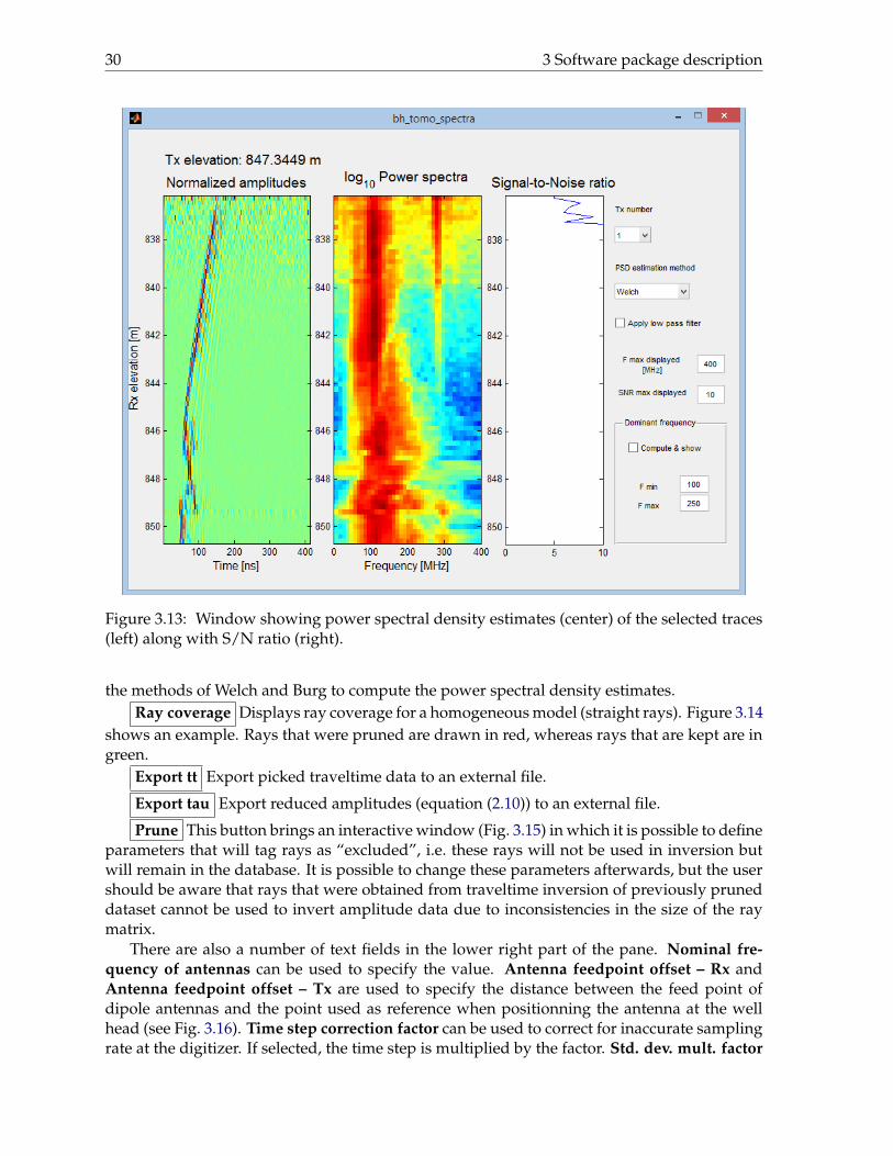
Figure 3.13: Window showing power spectral density estimates (center) of the selected traces(left) along with S/N ratio (right).

the methods of Welch and Burg to compute the power spectral density estimates.Ray coverage Displays ray coverage for a homogeneous model (straight rays). Figure 3.14

shows an example. Rays that were pruned are drawn in red, whereas rays that are kept are ingreen.

Export tt Export picked traveltime data to an external file.

Export tau Export reduced amplitudes (equation (2.10)) to an external file.

Prune This button brings an interactive window (Fig. 3.15) in which it is possible to defineparameters that will tag rays as “excluded”, i.e. these rays will not be used in inversion butwill remain in the database. It is possible to change these parameters afterwards, but the usershould be aware that rays that were obtained from traveltime inversion of previously pruneddataset cannot be used to invert amplitude data due to inconsistencies in the size of the raymatrix.

There are also a number of text fields in the lower right part of the pane. Nominal fre-quency of antennas can be used to specify the value. Antenna feedpoint offset – Rx andAntenna feedpoint offset – Tx are used to specify the distance between the feed point ofdipole antennas and the point used as reference when positionning the antenna at the wellhead (see Fig. 3.16). Time step correction factor can be used to correct for inaccurate samplingrate at the digitizer. If selected, the time step is multiplied by the factor. Std. dev. mult. factor


Figure 3.14: Ray coverage for a MOG dataset.

Figure 3.15: Utility window to prune MOG datasets.


Figure 3.16: Illustration of reference point and feed point of dipole antennas.

is a multiplier that is applied to the standard deviation of traveltime data. Finally, Date is thedate of data acquisition, which is used when processing time-lapse data.

3.2.3 Panels

Panels and super-panels are entities that are used to represent 2D cross-sections that are im-aged by the tomographic process. Super-panels are adjacent panels that can be juxtaposed.Currently, super-panels can be built only from panels made with vertical boreholes.

Add panel When the button Add is clicked in the Panels pane, a dialog is popped (Fig.3-14) that allows the user to enter a name for the panel to be created. By default, the panelname is automatically numbered incrementally.

Add MOG After a panel is created, MOG data must be tied to it. This is done by clickingthe Add button in the MOGs pane. A dialog window appears and the user must then selectone or more MOGs from the list.

Grid utility

Once the panels are defined, their inversion grids must be created. The program bh tomo grille,called from bh tomo db with the buttons in the Grid boxes, allows designing the grids. Usingbh tomo grille, it is possible to select the relative positioning of the boreholes, as well as thegrid step size and extents. It is also from bh tomo grille that the model constraints utilityis called. Adding constraints is possible only for regular panels, not super-panels.

3.2.4 General processing flow

Operations in bh tomo db should follow the following order:

1. Define boreholes;


Figure 3.17: Interactive screen of bh tomo grille.


Figure 3.18: Interactive screen of bh tomo tt.

2. Import MOG data. Optional steps are:

• Define air shots;

• Prune dataset.

3. Create panels, super-panels or 3D models.

3.3 Traveltime processing

3.3.1 Manual picking

Once data are imported in the database, the travel times can be picked with bh tomo tt. Inthis program, multi-offset gather (MOG) data are processed independently rather than on aper panel basis. As shown in Figure 3.18, the data are displayed in two windows: single tracesare shown on top, and all traces acquired for a given Tx position are drawn contiguously in thelower left box. This lower box allows a qualitative comparison of the picked times. The traveltimes for the air shots can also picked in bh tomo tt, by selecting the appropriate dataset inthe upper right part of the Control center box.

In bh tomo tt, it is possible to pick an interval of confidence (standard deviation) foreach trace. If standard deviations are picked, they will be used in the geostatistical inversion

3.3 Traveltime processing 35

to build the C0 matrix. The interval of confidence is a subjective parameter, and it is used togive more or less weight to the traveltime data during the inversion. It is thus important thatit is picked consistently, i.e. preferably by the same user.

Picking is normally done in the upper window, but it can also be done in the lower left box,albeit with less accuracy. When picking in the upper window, the user can choose between“picking with standard deviation” and “simple picking” in the popup menu on the right.Once picking is activated, each mouse button has a different function:

• left button to pick traveltime;

• center button to accept pick and go to next trace;

• right button to pick standard deviation.

Picking is deactivated by clicking outside the upper window.It is possible to view the arrival times and standard deviations as a function of the ray

length or ray angle by pressing the Statistics button. It is also possible to enhance the signalquality using a wavelet transform (WT) de-noising function. Note that this function requiresthe wavelet toolbox sold by the MathWorks. The filtering parameters are hard-coded in theprogram. Because of this, the original trace is shown in the background in light grey to ap-praise the quality of the filter when WT de-noising is selected. Note also that the picked timesare saved in the database and can be accessed at any time. Hence, picking sessions can beinterrupted and restarted afterwards. Finally, travel times picked in a third party software canbe imported in bh tomo tt (see appendix A.2 for file format).

3.3.2 Semi-automatic picking

The semi-automatick picking method is based on the work of Irving et al. (2007). Irving’salgorithm is based on the crosscorrelation of traces with a reference waveform for which thearrival time is known. The originality of the approach resides in the reference waveform be-ing obtained iteratively from the data set, through a specific sorting of the traces. First, thetraces are aligned using crosscorrelation with the reference trace being initially the one thathas the highest S/N ratio. The aligned traces are then stacked to produce a new referencewaveform, which is used to realign the traces. This process is repeated until all traces areproperly aligned. Finally, the arrival time is picked manually on the reference trace with thearrival times of the other traces determined from the crosscorrelation lags. The method is saidto be semi-automatic because the user must pick the reference trace and also intervene duringthe alignment of the traces in order to reject those that cannot be aligned properly.

To mitigate the effect of changes in the GPR phases on crosscorrelation, Irving et al. (2007)determine a number of different reference waveforms that represent ranges in transmitter/re-ceiver angle where the arriving pulses have similar shape. This is achieved by gathering thetraces by ray angle intervals. As illustrated in their paper, this step is essential in order toobtain high quality results. The main assumption behind this step is that waveforms recordedat similar angles have similar shapes. Irving et al. (2007) clearly point out that significantproblems may arise in situations where this assumption is violated, such as for data collectedabove the water table or near the surface, where sharp velocity contrasts, refracted arrivals,and changes in antenna coupling impact greatly on the waveforms and frequency content.


-1.2

-0.8

-0.4

0.0

0.4

0.8

1.2

Norm

alize

d am

plitu

de

20 30 40 50 60 70 80 90 100 110

Time [ns]

Original trace177 MHz synthetic waveletFiltered cycleTime window

Figure 3.19: Example of first-cycle isolation. The original trace, in blue, has a dominant fre-quency of 177 MHz. This trace is crosscorrelated with a 177 MHz synthetic wavelet, shown inred. After the application of the time window, the scattered arrivals are eliminated, as shownin green.

First-cycle isolation

To overcome the limitation of required waveform similarity, it is possible to preprocess thedata in a manner that isolates the first cycle of the GPR waveform (referred to as “first-cycleisolation”). By doing so, waveform similarity is increased and interference with scatteredarrivals during crosscorrelation can be avoided partly, if not completely. This step is typicallyapplied to traces with moderate to high S/N ratios because the scattered arrivals are usuallynot visible on traces with low S/N ratio. The preprocessing step proceeds as follows. Eachtrace is first normalized to its maximum absolute value. The traces are then crosscorrelatedwith a wavelet of the form (Arcone, 1991)

w(t) = sin (2p f t) sin2✓

2p f t4

◆with 0 t 2

f, (3.1)

where f is chosen to be the dominant frequency of the signal. To automate the procedure, thebeginning of the first cycle is picked at the first time lag exceeding a given crosscorrelationamplitude threshold, typically 0.25. A time window having a width slightly larger than thewavelet of equation 3.1 and beginning slightly before the above time lag datum is then appliedto nullify the undesired signals (see Figure 3.19). In this manner, we ensure that the soughtonset is not altered. The time window is extended with cosine tapers at the leading and trailingedges, to smooth out transitions. Note that the wavelet of equation 3.1 could be substitutedby any other that would be more adapted to the data at hand. However, since we only needto use a time window to suppress later arrivals and do not need to determine the onset timeitself, equation 3.1 works well enough.

Dominant frequency rescaling

Another problem that arises when using crosscorrelation for onset picking is that when thedominant frequencies of the wavelets vary, the widths of the wavelets vary and, therefore,they differ from the reference wavelet (left of Figure 3.20). An immediate consequence is thatthe crosscorrelation lags will not fall exactly at the onset, leading to an error in the picked time.

3.3 Traveltime processing 37

-1.00

-0.75

-0.50

-0.25

0.00

0.25

0.50

0.75

1.00

Norm

alized a

mplitu

de

50 75 100 125 150

Time [ns]

fd 109 MHz

fd 78 MHz

fd 63 MHz

Stacked reference

-1.00

-0.75

-0.50

-0.25

0.00

0.25

0.50

0.75

1.00

Norm

alized a

mplitu

de

75 100 125 150 175

Time [ns]

109 MHz rescaled

78 MHz rescaled

63 MHz rescaled

Stacked reference

Figure 3.20: Illustration of the effect of time rescaling for three synthetic traces having differentdominant frequencies. The traces are aligned without (left) and with (right) time rescaling.

To help minimize this problem, the ability to stretch the first cycles to a common length hasbeen added to the procedure. This is done by rescaling the time scale of each trace by the ratiof id/ f , where f i

d is the dominant frequency of the ith trace and fd is the average of the dominantfrequency for all traces. Because the crosscorrelation picking procedure requires that the timescales be consistent, all the stretched traces must be interpolated to a common time scale.An example of the results obtained with this procedure is shown in Figure 3.20, illustratingthe improved similarity between the rescaled traces and the reference obtained after stacking.Finally, note that after completion of the picking procedure, the obtained times are scaled backto their original time frames.

User interface

The module that allows performing semi-automatic picking is bh tomo pick. The user’sinterface is shown in Figure 3.21. The steps to follow to process the data are:

1. Load MOG data, choose bin width;

2. Optionaly select wether first-cycle isolation and/or dominant frequency rescaling shouldbe applied. If so, press the Prepare button to process the data accordingly. These pro-cessing steps are restricted to traces with signal to noise ratio above the values specifiedin the “Traces” box. Finally, in first cycle isolation, it is possible to combine the isolatedcycle with the original trace by giving a weight less than 1 in the field named Weight -traces 1 cycle.

3. For each bin:

(a) align traces by pressing Align traces ; repeat as necessary;

(b) Pick the traveltime and standard deviation of the reference trace. Picking is acti-vated by pressing Pick mean trace . The mouse buttons have the same effect asdescribed in section 3.3.1.

4. After all bins have been processed and reference traces been picked, perform automaticpicking of the remaining traces by pushing Pick traces using cross correlation .

5. Save your work.

Quality control can be done afterwards in bh tomo tt.


Figure 3.21: Interactive screen of bh tomo pick.

3.4 Amplitudes processing 39

3.3.3 Automatic picking

Automatic picking method is based on the Akaike information criterion (AIC) and continuouswavelet transform (CWT). The window of Automatic picking module is shown in fig XXX

Different wave types can be present in a radar trace. Hence, similarity between tracesrecorded at different locations is never guaranteed. It is therefore appealing to have an au-tomatic picking method that does not rely on waveform similarity. For this reason, the AICpicker is chosen as a starting basis because of its simplicity and efficiency. CWT is used tocorrect the ACI to obtain a higher level of accuracy of picking.

The approaches can be summarised as following:1). After pre-processing the data, the traces are truncated in time at their maximum ampli-

tude, the AIC is calculated on all truncated traces; the onset picking is determined by findingthe AIC minimum.

2). For each trace, the dominant frequency of the radar wavelet is calculated and then usedto scale the complex wavelet transform. If the dominant frequency cannot be fond with theprocedure, the frequency at the maximum of the amplitude spectrum is taken.

3). The position of the first break of radar wavelet is extracted from the phase part of thecomplex wavelet transform. Then, ensure the CWT correction falls near the ACI peak.

4). After all traces are processed, common-receiver-gather plots with associated first-arrivalpicks and uncertainties are displayed.

3.4 Amplitudes processing

Similarly, bh tomo amp can be used to process the amplitude data. Like in bh tomo tt,multi-offset gather data are processed independently rather than on a per panel basis. Inbh tomo amp, the user selects a time window into which the analysis is carried out. Also,upon user selection, peak-to-peak amplitude or centroid frequency is computed. In the latercase, the frequency spectrum can be computed using a simple FFT after application of a Han-ning window to the selected portion of the trace, or using the S-transform (Stockwell et al.,1996). The S-transform gives a joint time-frequency representation of the signal, similar tothe continuous wavelet transform, but which retains a direct relationship with the Fourierspectrum. To compute the centroid frequency with the S-transform, the spectrum with maxi-mum energy in the selected time window is used. An example is shown in Fig. 3.22. A traceis shown in the upper part and its corresponding time-frequency spectrum is shown in thelower left box. In this case, the selected time window is [45-63] ns. The frequency spectrumwith maximum energy in this interval is used to compute fr and s2

R.When saving the data, the amplitudes or centroid frequencies are reduced to pseudo travel

times (t in Eq. 2.9 or Eq. 2.15). To perform this transformation, the length of the rays must beknown. Straight rays are computed by default. However, it is possible to load rays that weretraced after the inversion of travel times by pressing the appropriate button (see Fig. 3.22).During the saving process, a small utility is launched to view and manually adjust A0 or fS.Prior to saving, it is possible to discard the traces for which the ray are departing or arrivingwith small angles at the antennas. This is done by adjusting the minimum angle value in thespecified box. If curved rays are loaded, the traces for which the first arrival is refracted onsurface are also rejected. If this is not desirable, the user must specify a value of “Z surface”higher than the highest elevation attained by the rays.

Note that in bh tomo amp, each trace datum can be weighted by the inverse of the signal-


Figure 3.22: Interactive screen of bh tomo amp.

to-noise ratio (S/N) by selecting the Weighting 1/(S/N) button. In such case, the inverse ofS/N is taken as the standard deviation in the covariance model. However, there is no physicalmeaning to this so-called standard deviation, and our experience showed that this feature doesnot produce good results. At this point, it is therefore not recommended to select this option.

3.5 Fitting the model covariance

Once the travel times are picked, a slowness covariance model (Cov(s, s)) must be chosen toperform the geostatistical inversion. The covariance Cov(s, s) is obtained through Eq. (2.24).However, the covariance Cov(t⇤, t⇤) is not stationary. Therefore, estimators such as traditionalvariogram or covariogram cannot be used directly, and the model parameters for slownesscovariance must be estimated by inversion. The program bh tomo fitCovar is designed ac-complish this task interactively using the concept of the V-V plot described in Asli et al. (2000),or automatically using a minimization scheme based on the Simplex method implementationof Matlab. In the V-V plot approach, the theoretical covariance values are sorted in decreasingorder and bined in classes for which the mean value is calculated. The same sorting orderand bining scheme is applied to the experimental data. Thus, a value corresponding roughlyto a single theoretical structural distance can be calculated for an experimental variogram.If the chosen slowness covariance model is appropriate, the experimental variogram versustheoretical variogram plot (the V-V plot) should show a dispersion around a line at 45�.

Contrary to bh tomo tt and bh tomo amp in which the MOG data are processed inde-pendently, the calculations made in bh tomo fitCovar are done with the entire data of a

3.6 Inversion 41

Figure 3.23: Interactive screen of bh tomo fitCovar.

panel or super-panel. If the panel contains more than one MOG dataset, they are merged to-gether. The interface of bh tomo fitCovar, shown in Fig. 3.23, comprises two boxes wherethe experimental covariance, Cov(t⇤, t⇤), can be visually compared with the theoretical modelL Cov(s, s) LT + C0. The upper box is the V-V plot, whereas the sorted bined covariances areshown in the lower box. The covariance model parameters can be set manually, or, as statedpreviously, adjusted automatically using a minimization scheme based on a Simplex methodimplementation. The covariance model can include up to two elementary structures and anugget effect on slowness. A nugget effect on traveltime can also be specified. Note that inorder to speed up the calculations, bins with low covariance values can be discarded by givinga value below 1 for the fraction of bins (typically 0.25 to 0.5 is sufficient). Note also that the raymatrix L can be given in input, for example in the case where amplitude data are processed.When processing time data, matrix L is not known unless a prior inversion has been carriedout, for example using only straight rays. However, our experience indicates that generally,using straight rays yields adequate estimates of the covariance model.

3.6 Inversion

The program covered in this section is bh tomo inv, in which the tomographic inversion isperformed. The interface is shown in Fig. 3.24. Both travel time and amplitude data can beinverted, provided that proper processing has been carried out. As a mean of control, the


Figure 3.24: Interactive screen of bh tomo inv. Two velocity models obtained with the datapresented in section 4 are displayed. The leftmost model is obtained by cokriging and therightmost model is the simulation that best fits the data.

travel time and amplitude data can be viewed using the Data menu items. Various parametersaffecting the inversion can be set, notably the use of the model constraints and the use ofpreviously calculated rays. The choice between geostatistical and LSQR algorithm is also madein bh tomo inv. Depending on the type of algorithm, the appropriate parameters that canbe adjusted are displayed in the bottom left frame. The parameters for LSQR are describedin appendix B. In the case of geostatistical inversion, only the covariance model needs to begiven (it is loaded automatically if bh tomo fitCovar has been used). The covariance modelparameters can be modified by the user. When performing LSQR inversion, a starting modelcan be built interactively using a GUI accessible from the Inversion-Initial model menu item.In the case of geostatistical inversion, the starting model is always homogeneous.

The number of straight and curved rays iterations is given in the upper part of the Datapane. When performing geostatistical inversion of traveltime data, one iteration of each usu-ally suffice. When geostatistical inversion of amplitude data is performed, curved rays previ-ously obtained from traveltime inversion can be used. The list of previous inversions savedin the database appears in the upper left popup menu of the “Previous inversion” pane. Theuser can select which inversion should be used by choosing the appropriate item in the list andactivate the “Use rays” checkbox. Note that when performing geostatistical inversion of am-plitude data, the ray matrix should note be updated, i.e. the number of curved ray iterationsmust always be equal to 0.

3.7 Estimating the saturation of the magnetic nanofluid 43

The inversion is started by pressing the Inversion button. After completion, the resultscan be saved in the database for later retrieval, using the File-Save menu item, or exported ina separate mat-file. The format of this file is given in appendix A.4. The inversion parametersare saved together with the results. The inversion results and ray coverage can be viewed inseparate windows by calling the appropriate Results menu item. When geostatistical simu-lations are carried out, all simulated fields are saved after completion of the inversion. If noconstraints are imposed, the “best” simulated field is the one obtained after gradual deforma-tion of all simulated fields. In the gradual deformation method, the realizations are combinedsequentially, two at a time, with weights chosen as to maximize a goodness of fit criterion(Hu, 2002). This method has proven its efficiency in petroleum applications. In the case whereconstraints are applied, the gradual deformation scheme cannot be used directly because oneworking hypothesis of the method is that the simulated fields have a Gaussian distributionwith zero mean. When the properties of air (above the surface) are fixed, the distribution ofthe properties is no longer Gaussian. In this case, the “best” simulated field is the one thatminimizes the L1 norm of the residuals.

3.7 Estimating the saturation of the magnetic nanofluid

3.7.1 Background

Tomographic measurements allow mapping the velocity and attenuation of radio frequencyEM waves in the ground. The attenuation and velocity are expressed in terms of physicalproperties by

a = wp

µe

vuut12

"r1 +

⇣ s

we

⌘2� 1

#, (3.2)

v =

8<

:p

µe

vuut12

"r1 +

⇣ s

we

⌘2+ 1

#9=

;

�1

, (3.3)

where w is the angular frequency, µ is the magnetic permeability, e is the dielectric permittivityand s is the electric conductivity. The injection of the magnetic nano fluid will change thephysical properties of the reservoir rock and thus affect the velocity and attenuation of the EMwave propagating in that reservoir. In this section we show how can EM measurements allowmapping and retrieving the quantity of injected nano fluid.

Using a time-lapse approach, the available data are v1, a1, v2 and a2, where subscript 1indicates baseline data and subscript 2 repeat data. The idea is to combine the time-lapse dataand petrophysical relationships to infer the saturation of the magnetic nano fluid at the timeof the repeat survey. The saturation, noted S, is defined as the volumetric proportion of themagnetic fluid.

A number of assumptions must be used to infer S. We first assume that there is no magneticmaterial in the earth at baseline, i.e. µ1 is equal to the magnetic permeability of vacuum (µ0).We also assume that the physical properties of the rock are known: the permittivity of the rockmatrix em is known as well as the Archie parameters a and m are known. Finally, the propertiesof the nano fluid (sn f , en f and µn f ) are also assumed to be known. It is also possible to assumethat the properties of the reservoir fluid are known, e.g. from well sampling; if this is not thecase, the porosity of the reservoir must be known.


In the case where the porosity is known, we can infer the properties of the fluid in placebefore injection (sf1 and e f1 ) from v1 and a1. First get the values for the rock-fluid mixture (s1and e1):

e1 =1µ0

✓1v2

1� a2

1w2

◆; (3.4)

s1 =2a1

µ0v1. (3.5)

Using Archie’s equation (Schon, 2004), the conductivity of the fluid is

sf1 = as1f�m. (3.6)

The permittivity of the rock-fluid mixture is generally described by the self-similar model ofSen et al. (1981)

e1 � em

e f1 � em

✓e f1

e1

◆Y= f, (3.7)

where Y is the depolarization factor, assumed equal to 1/3. This equation must be solvednumerically. The self-similar model is also used to compute the conductivity and permeabilityof the rock-fluid mixture (Mavko et al., 2009). When the properties of the fluid are known, theporosity can be calculated using (3.6) and (3.7) and averaged.

After injection, the magnetic permeability of the medium is no longer equal to µ0, and wehave

e2 =1µ2

✓1v2

2� a2

2w2

◆; (3.8)

s2 =2a2

µ2v2. (3.9)

There are thus three unknowns (s2, e2 and µ2), but only two equations. Also, the fluid is amixture of the initial fluid and the magnetic fluid. The aim is to isolate S from these equationsand known petrophysical relationships.

The electric conductivity of the fluid mixture after injection can be described by the self-similar model

sf2 � sf1

sn f � sf1

✓sn f

sf2

◆Y= S. (3.10)

The conductivity of the saturated rock is then

s2 =1a

sf2 fm. (3.11)

Because the nano fluid is the only magnetic material, the permeability of the medium afterinjection is

µ2 � µ0

µn f � µ0

✓µn f

µ2

◆Y= Sf. (3.12)

In the case of permittivity, the expression for the fluid mixture is

e f2 � e f1

en f � e f1

✓en f

e f2

◆Y= S, (3.13)


Fluid s (S/m) e (eo) µ (µo)nano fluid 0.01 75 3oil 0.001 2.25 1brine 1 76 1

Table 3.1: Physical properties of fluids

and the expression for the saturated rock is

e2 � em

e f2 � em

✓e f1

e2

◆Y= f. (3.14)

Unfortunately, all the expressions above preclude finding a closed-form expression for S.The proposed approach for solving the problem is to use a global optimization algorithm. Theconstrained simulated annealing is adopted here (Kirkpatrick et al., 1983; Press et al., 1992),where the problem is constrained such that 0 S 1. The input parameters are the measureddata v1, a1, v2 and a2, as well as the known properties em, f, a, m, sn f , en f and µn f . The stepsare

1. compute e f1 and sf1 , or evaluate f.

2. start with a guess value S0.

3. iterations:

• compute e f2 and sf2 ;• compute µ2, e2 and s2;• compute estimates of velocity and attenuation v2 and a2;• update S with the simulated annealing algorithm.

Implementation and validation

The proposed algorithm has been implemented in matlab and incorporated in bh tomo. Theself-similar model is solved with the matlab function fsolve which by default uses the trust-region-dogleg algorithm. This function is used by the function findS.m that allows estimat-ing the saturation. The function simulannealbnd of the global optimization toolbox is at thecore of the function.

The code has been validated by testing four scenarios. Two types of rock are considered:carbonates and sandstone, which are distinguished by their relative dielectric permittivity val-ues (respectively 8 and 4.65). For both types of rock, the scenarios where oil and brine aresubstituted by the magnetic nanofluid are evaluated. In the four cases, the porosity of thereservoir is 20%, the Archie parameters a and m are equal to 0.62 and 1.72 respectively, thedepolarization factor Y is 1/3, and the calculations are done for a frequency of 50 MHz. Theproperties of the fluids are given in Table 3.1.

The first test were carried out by feeding the program with the true values of fluids androck matrix properties, and also assuming that the EM wave velocity and attenuation are ex-actly known. In all cases, the starting value of S was 0.5. Figure 3.25 show the fit betweenthe estimated saturations and the true saturations. For each case, the norm of relative error(dS = DS/S, for S > 0) is indicated in the sub-figures. The results are excellent, with kdSk


0 0.1 0.2 0.3 0.4 0.5 0.6 0.7 0.8 0.9 10

0.1

0.2

0.3

0.4

0.5

0.6

0.7

0.8

0.9

1

True saturation

Est

imate

d s

atu

ratio

n

Carbonate with oil (||δ S|| = 2.361 %)

0 0.1 0.2 0.3 0.4 0.5 0.6 0.7 0.8 0.9 10

0.1

0.2

0.3

0.4

0.5

0.6

0.7

0.8

0.9

1

True saturation

Est

imate

d s

atu

ratio

n

Carbonate with brine (||δ S|| = 0.232 %)

0 0.1 0.2 0.3 0.4 0.5 0.6 0.7 0.8 0.9 10

0.1

0.2

0.3

0.4

0.5

0.6

0.7

0.8

0.9

1

True saturation

Est

imate

d s

atu

ratio

n

Sandstone with oil (||δ S|| = 0.883 %)

0 0.1 0.2 0.3 0.4 0.5 0.6 0.7 0.8 0.9 10

0.1

0.2

0.3

0.4

0.5

0.6

0.7

0.8

0.9

1

True saturation

Est

imate

d s

atu

ratio

n

Sandstone with brine (||δ S|| = 0.138 %)

Figure 3.25: Accuracy of the saturation estimates with exact input parameters.

varying between 0.05 and 2.4%. Obviously, in real-life situations the fluid and rock propertieswill be known only approximately, as will be the case for velocity and attenuation inferredby tomographic measurements. To assess the effect of inaccuracies in the estimation of thelatter two parameters, the carbonate/oil scenario above was repeated with v1 and v2 under-estimated and overestimated by 5%. Feeding the estimation routine with these values resultsin errors growing dramatically as function of S, as shown in Figure 3.26. The same exercisewas repeated with a1 and a2 underestimated and overestimated by 20%. Such a large valuewas chosen because amplitude tomography is much less accurate than traveltime tomogra-phy (Giroux and Chouteau, 2006). We can see however in Figure 3.26 that a has less impacton estimating the saturation, which is positive given that we have less grasp on estimating a.Nevertheless, the relative error becomes important for S > 0.5 and being in position to rely onaccurate maps of a and v appears crucial.

3.7.2 User interface


0 0.1 0.2 0.3 0.4 0.5 0.6 0.7 0.8 0.9 10

0.1

0.2

0.3

0.4

0.5

0.6

0.7

0.8

0.9

1

True saturation

Est

imate

d s

atu

ratio

n

v underestimated (||δ S|| = 146.2 %)

0 0.1 0.2 0.3 0.4 0.5 0.6 0.7 0.8 0.9 10

0.1

0.2

0.3

0.4

0.5

0.6

0.7

0.8

0.9

1

True saturation

Est

imate

d s

atu

ratio

n

v overestimated (||δ S|| = 93.6 %)

0 0.1 0.2 0.3 0.4 0.5 0.6 0.7 0.8 0.9 10

0.1

0.2

0.3

0.4

0.5

0.6

0.7

0.8

0.9

1

True saturation

Est

imate

d s

atu

ratio

n

α underestimated (||δ S|| = 26.4 %)

0 0.1 0.2 0.3 0.4 0.5 0.6 0.7 0.8 0.9 10

0.1

0.2

0.3

0.4

0.5

0.6

0.7

0.8

0.9

1

True saturation

Est

imate

d s

atu

ratio

n

α overestimated (||δ S|| = 23.1 %)

Figure 3.26: Accuracy of the saturation estimates for inaccurate velocity and attenuation inputdata.


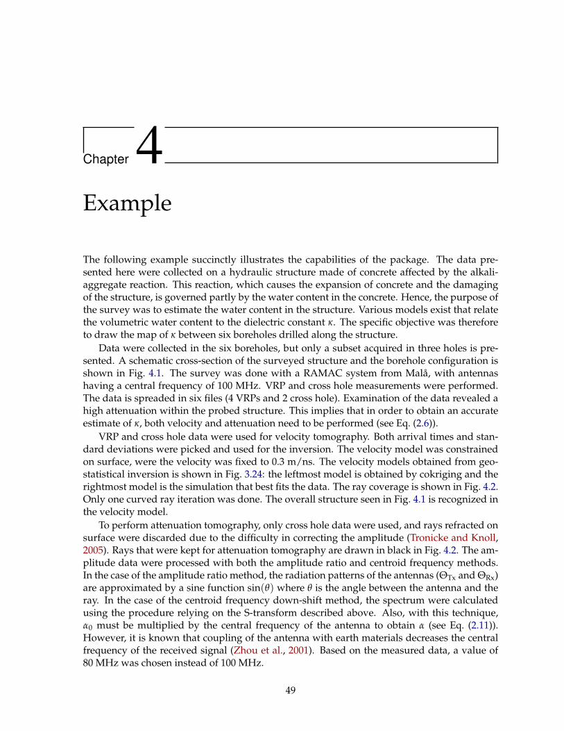
Chapter 4Example

The following example succinctly illustrates the capabilities of the package. The data pre-sented here were collected on a hydraulic structure made of concrete affected by the alkali-aggregate reaction. This reaction, which causes the expansion of concrete and the damagingof the structure, is governed partly by the water content in the concrete. Hence, the purpose ofthe survey was to estimate the water content in the structure. Various models exist that relatethe volumetric water content to the dielectric constant k. The specific objective was thereforeto draw the map of k between six boreholes drilled along the structure.

Data were collected in the six boreholes, but only a subset acquired in three holes is pre-sented. A schematic cross-section of the surveyed structure and the borehole configuration isshown in Fig. 4.1. The survey was done with a RAMAC system from Mala, with antennashaving a central frequency of 100 MHz. VRP and cross hole measurements were performed.The data is spreaded in six files (4 VRPs and 2 cross hole). Examination of the data revealed ahigh attenuation within the probed structure. This implies that in order to obtain an accurateestimate of k, both velocity and attenuation need to be performed (see Eq. (2.6)).

VRP and cross hole data were used for velocity tomography. Both arrival times and stan-dard deviations were picked and used for the inversion. The velocity model was constrainedon surface, were the velocity was fixed to 0.3 m/ns. The velocity models obtained from geo-statistical inversion is shown in Fig. 3.24: the leftmost model is obtained by cokriging and therightmost model is the simulation that best fits the data. The ray coverage is shown in Fig. 4.2.Only one curved ray iteration was done. The overall structure seen in Fig. 4.1 is recognized inthe velocity model.

To perform attenuation tomography, only cross hole data were used, and rays refracted onsurface were discarded due to the difficulty in correcting the amplitude (Tronicke and Knoll,2005). Rays that were kept for attenuation tomography are drawn in black in Fig. 4.2. The am-plitude data were processed with both the amplitude ratio and centroid frequency methods.In the case of the amplitude ratio method, the radiation patterns of the antennas (QTx and QRx)are approximated by a sine function sin(q) where q is the angle between the antenna and theray. In the case of the centroid frequency down-shift method, the spectrum were calculatedusing the procedure relying on the S-transform described above. Also, with this technique,a0 must be multiplied by the central frequency of the antenna to obtain a (see Eq. (2.11)).However, it is known that coupling of the antenna with earth materials decreases the centralfrequency of the received signal (Zhou et al., 2001). Based on the measured data, a value of80 MHz was chosen instead of 100 MHz.

49

50 4 Example

0 m

15 m

10 m

5 m

1 m

1 2 3

Rock Water table

Concrete Porous cement paste

Backfill Mortar

Figure 4.1: Schematic cross-section of the surveyed structure interpreted from boring logs.

For both datasets, the inversion parameters were the same: identical covariance model,model constrained on surface (a = 0 above the ground), and 128 simulations to perform. Theresults of the simulations are shown in Figs. 4.3 and 4.4. These figures show the simulation thatbest fits the reduced data (L1 norm), as well as the standard deviation of the model parametercomputed from the 128 simulated attenuation fields. Both datasets yield very similar results,although the average attenuation is slightly lower in the case of the centroid frequency dataset.

Dielectric constant and electric conductivity maps computed with equations (2.6) and (2.7)are shown in Fig. 4.5. The best-fit simulation results were used, and attenuation obtained withthe centroid frequency down-shift method was selected. These maps were constructed outsidebh tomo, after the data have been exported from bh tomo. They show different anomalies,especially in the backfill, at the backfill/concrete interface, and between Holes 2 and 3.

51

0 2 4

-15

-10

-5

0

Ray coverage

Distance [m]

Ele

vati

on

[m]

Figure 4.2: Ray coverage for the velocity model shown in Fig. 3.24. Grayed out rays wereexcluded for attenuation tomography.

52 4 Example

Attenuation [Np/m]

Distance [m]

Ele

vati

on

[m

]

0 2 4 6

-15

-10

-5

0

0

0. 5

1

1. 5

2

2. 5

0.02

0.04

0.06

0.08

0. 1

0.12

0.14

Amplitude ratioStandard deviation

Distance [m]0 2 4 6

-15

-10

-5

0

Figure 4.3: Simulation results of the geostatistical inversion of amplitude data, amplituderatio method. On the left: simulation that best fits the data. On the right: standard deviationinfered from the 128 simulations.

53

Attenuation [Np/m]

Distance [m]

Elev

atio

n [m

]

0 2 4 6-15

-10

-5

0

0

0. 5

1

1. 5

2

2. 5

0.02

0.04

0.06

0.08

0. 1

0.12

0.14

Centroid frequencyStandard deviation

Distance [m]0 2 4 6

-15

-10

-5

0

Figure 4.4: Simulation results of the geostatistical inversion of amplitude data, centroid fre-quency down-shift method. On the left: simulation that best fits the data. On the right: stan-dard deviation infered from the 128 simulations.

54 4 Example

Dielectric constant

Distance [m]

Ele

vati

on

[m]

0 2 4 6-15

-10

-5

0

2

4

6

8

10

12

14

0

5

10

15

20

25

30

35

40

Physical propertiesConductivity [mS/m]

Distance [m]0 2 4 6

-15

-10

-5

0

1 32 1 32

Figure 4.5: Maps of dielectric constant and effective electric conductivity infered from thetomographic results. Boreholes 1, 2 and 3 are drawn in green.

Appendix AExchange files formats

bh tomo modules can import or export various data in different formats. Data that can beimported are picked travel times (in bh tomo tt), and slowness or attenuation constraints (inbh tomo contraintes). Data that can be exported are the inversion results (from bh tomo inv).Note that all data are stored in the mini database which is one large mat-file that can be loadedat any time in Matlab.

A.1 Aramco’s Magnetic NanoMappers data

A.1.1 Motivation for the format

The purpose of the format is to have all information needed to perform traveltime and ampli-tude tomography easily accessible. A single struct variable is used, with appropriate fieldsfor each parameter. The data can then be imported in matlab with a single load command.The name of the struct variable is chosen to be data.

Definitions

bh tomo was first developed for processing borehole ground-penetrating-radar data. Manyparameters are related to borehole GPR antennas and data acquisition. Figure 3.6 illustratestwo common survey modes, namely the multi-offset gather and vertical radar profiling.

Description of the fields

Table A.1 lists the fields of the struct variable and gives a short description.Note that the date can be edited in the database GUI (bh tomo db).

Important For data acquired in a well (MOG survey), the Z coordinate of transmitter andreceiver are the depth (positive downward) from the collar of the well, or kelly bushing or anyother reference elevation on surface. For VRP survey configuration, the Tx is on surface andmoved away from the well head (where receivers are) along a line pointing toward a secondwell. The Z coordinates of the Tx correspond to the distance from well, as shown in Figure 3.7.

55

56 A Exchange files formats

Name Size Descriptionntrace 1 Number of traces in the filenptsptrc 1 Number of points per tracetimec 1 Sampling periodtimestp 1⇥nptsptrc Time axis datardata nptsptrc⇥ntrace Trace dataTx x 1⇥ntrace X coordinate of transmitterTx y 1⇥ntrace Y coordinate of transmitterTx z 1⇥ntrace Z coordinate of transmitterRx x 1⇥ntrace X coordinate of receiverRx y 1⇥ntrace Y coordinate of receiverRx z 1⇥ntrace Z coordinate of receiverrstepsz 1 Distance along well between two measurementsTxOffset 1 Offset between antenna head and feed pointRxOffset 1 Offset between antenna head and feed pointantennas string Antenna typernomfreq 1 Nominal frequency of the antennas (MHz)synthetique 1 0 for real data, 1 for modelled tracescunits string Distance unitstunits string Time unitscsurvmod string Survey Mode, either ’MOG’ or ’VRP’date string Date of data acquisition in the field

Table A.1: Fields of the struct variable

In the current 2D version, X and Y coordinates are not used. The coordinates are projectedalong the well trajectory. If one does not want the coordinates to be interpolated, a string vari-able comment equal to ’true positions’ should be added to data.

An example of the content of the struct variable is given below:

A.2 Picked arrival times 57

>> data

data =

ntrace: 945nptsptrc: 512

timec: 0.8012timestp: [1x512 double]

rdata: [512x945 double]Tx_x: [1x945 double]Tx_y: [1x945 double]Tx_z: [1x945 double]Rx_x: [1x945 double]Rx_y: [1x945 double]Rx_z: [1x945 double]

rstepsz: 0.2493TxOffset: 0.6650RxOffset: 0.6650antennas: ’100 MHz Borehole - Ramac’rnomfreq: 100

synthetique: 0cunits: ’m’tunits: ’ns’

csurvmod: ’SURVEY MODE = Trans. - MOG’date: ’15-Oct-2012’

The first trace can be displayed by issuing the command at the matlab prompt:plot(data.timestp,data.rdata(:,1)).

A.2 Picked arrival times

Arrival times picked in a third party software can be imported in bh tomo tt. The pickedtimes must correspond to the multi-offset gather data file being processed. They must bestored in an ASCII file, formatted in two or three columns. The first column is the trace numberin the current MOG data file and the second column is the picked time. An optional thirdcolumn contains the standard deviation of the corresponding arrival time.

A.3 Model constraints

Similarly to the arrival times, constraints in the velocity or attenuation models can be importedin bh tomo contraintes (this program is accessible from bh tomo db via the grid utilities).The constraints must also be stored in an ASCII file, in three columns: the first column containsthe elevations and the second column contains the horizontal distances relative to the gridorigin where to insert the constraint values, which are included in the third column.

58 A Exchange files formats

A.4 Inversion results

The results of inversion runs can be exported in a Matlab mat-file from bh tomo inv. Thisfiles contains two structured variables: param and tomo. The fields of the variable paramcorrespond to the inversion parameters, whereas the fields of the variable tomo are the inver-sion results. The fields of tomo are detailed in Table A.2. Note that some fields might not bepresent, depending on the type of inversion carried out, i.e. LSQR vs geostatistical, with orwithout simulations.

Table A.2: Description of the fields of the structured variable tomo

Name Type Size Descriptionrais cell array 1⇥ no Each element of the cell array contains a n ⇥ 3 matrix of the n � 1 ray segments

coordinates.L matrix no ⇥ np Matrix L of Eq. (2.3)no trace matrix no ⇥ 1 Trace number in the database for each of the no observationss matrix np ⇥ 1 Slowness or attenuation fieldsimu matrix np ⇥ nsimu Simulated slowness or attenuation fieldsgr matrix np ⇥ 1 Simulated slowness or attenuation field after gradual deformationx matrix nx ⇥ 1 Horizontal coordinates of the center of the grid cellsz matrix nz ⇥ 1 Elevation coordinates of the center of the grid cellslmoy scalar – Mean slowness or attenuationdiff1 matrix 1⇥ nsimu Fit of the simulated slowness or attenuation fields to the datadiff1 min scalar – Number of the simulated slowness or attenuation field that fits best the datadt matrix no ⇥ 1 Data (centered)

Appendix BLSQR inversion parameters

The parameters that can be adjusted by the user when using the LSQR algorithm are definedin Table B.1.

Table B.1: Description of the LSQR inversion parameters

Name DescriptionTolerance Iterations stopped if L2 norm of the residuals lower than Tolerance.alpha Lagrange multiplier of the smoothing operator (second derivative).gradmin Iterations stopped if gradient of the L2 norm of the residuals lower than gradmin.correlmin Iterations stopped if correlation of models between iterations is higher than

correlmin.Nb of iterations Maximum number of iterations.Max vel. variation per it. Maximum variation of velocity in percent that is allowed at each iteration. If ex-

ceeded, the velocity perturbation is rescaled to this maximum.

59

60 B LSQR inversion parameters

Bibliography

Arcone, S. A. (1991). Dielectric constant and layer-thickness interpretation of helicopter-borneshort-pulse radar waveforms reflected from wet and dry river-ice sheets. IEEE Transactionson Geosciences and Remote Sensing, 29(5):768–777. 36

Asli, M., Marcotte, D., and Chouteau, M. (2000). Direct inversion of gravity data by cokriging.In Kleingeld, W., editor, Geostat2000 - Proceedings of the International Geostatistics Congress,Cape Town. 14, 40

Bai, C.-Y., Greenhalgh, S., and Zhou, B. (2007). 3D ray tracing using a modified shortest-pathmethod. Geophysics, 72(4):T27–T36. 17

Beaty, K. S., Perron, G., Kay, I., and Adam, E. (2002). DSISoft–a MATLAB VSP data processingpackage,. Computers and Geosciences, 28(4):501–511. 7

Cai, W., Qin, F., and Schuster, G. T. (1996). Electromagnetic velocity inversion using 2-DMaxwell’s equations. Geophysics, 61(4):1007–1021. 9

Chapman, B., Jost, G., and van der Pas, R. (2007). Using OpenMP: Portable Shared MemoryParallel Programming. MIT Press. 20

Chiles, J.-P. and Delfiner, P. (1999). Geostatistics: Modeling Spatial Uncertainty. John Wiley &Sons. 14

Conroy, J. P. and Radzevicius, S. J. (2003). Compact MATLAB code for displaying 3D GPR datawith translucence. Computers and Geosciences, 29(5):679–681. 7

Cormen, T. H., Leiserson, C. E., Rivest, R. L., and Stein, C. (2009). Introduction to Algorithms.MIT Press, 3rd edition. 18

Ernst, J., Maurer, H., Green, A., and Holliger, K. (2007). Full-waveform inversion of crossholeradar data based on 2-d finite-difference time-domain solutions of maxwell’s equations. Geo-science and Remote Sensing, IEEE Transactions on, 45(9):2807–2828. 9

Giroux, B. and Chouteau, M. (2006). On the processing of borehole georadar data for ray-basedattenuation tomography. In Daniels, J. J. and Chen, C.-C., editors, Proceedings of the EleventhInternational Conference on Ground-Penetrating Radar, number BOR.5, Columbus, Ohio, USA.GPR2006. 46

61

http://dx.doi.org/10.1109/36.83992

http://dx.doi.org/10.1190/1.2732549

http://dx.doi.org/10.1016/S0098-3004(01)00073-5

http://dx.doi.org/10.1190/1.1444023

http://dx.doi.org/10.1016/S0098-3004(03)00047-5

http://dx.doi.org/10.1109/TGRS.2007.901048

62 BIBLIOGRAPHY

Giroux, B. and Chouteau, M. (2010). Quantitative analysis of water-content estimationerrors using ground-penetrating radar data and a low-loss approximation. Geophysics,75(4):WA241–WA249. 11

Giroux, B., Gloaguen, E., and Chouteau, M. (2004). Geotechnical application of borehole GPR– a case history. In Slob, E. and Yarovoy, A., editors, Tenth International Conference on Ground-Penetrating Radar, pages 249–252, Delft, The Netherlands. TUDelft. 7

Gloaguen, E., Marcotte, D., Chouteau, M., and Perroud, H. (2005). Borehole radar velocityinversion using cokriging and cosimulation. Journal of Applied Geophysics, 57(4):242–259. 7,13, 14

Gruber, T. and Greenhalgh, S. A. (1998). Precision analysis of first-break times in grid models.Geophysics, 63(3):1062–1065. 17

Holliger, K., Musil, M., and Maurer, H. R. (2001). Ray-based amplitude tomography for cross-hole georadar data: a numerical assessment. Journal of Applied Geophysics, 47:285–298. 11

Hu, L. Y. (2002). Combination of dependent realizations within the gradual deformationmethod. Mathematical Geology, 34(8):953–963. 43

Hubbard, S. S., Peterson, J. E., Majer, E. L., Zawislanski, P. T., Williams, K. H., Roberts, J., andWobber, F. (1997). Estimation of permeable pathways and water content using tomographicradar data. The Leading Edge, 16(11):1623–1628. 7

Huisman, J. A., Hubbard, S. S., Redman, J. D., and Annan, A. P. (2003). Measuring soil watercontent with ground penetrating radar: A review. Vadose Zone Journal, 2:476–491. 10

Irving, J. D., Knoll, M. D., and Knight, R. J. (2007). Improving crosshole radar velocity tomo-grams: A new approach to incorporating high-angle traveltime data. Geophysics, 72(4):J31–J41. 35

Josuttis, N. M. (2012). The C++ Standard Library: A Tutorial and Reference. Addison Wesley, 2nd

edition. 18, 19

Kirkpatrick, S., Gelatt Jr., C. D., and Vecchi, M. P. (1983). Optimization by simulated annealing.Science, 220:671–680. 45

Le Ravalec, M., Noetinger, B., and Hu, L. Y. (2000). The FFT moving average (FFT-MA) gener-ator: An efficient numerical method for generating and conditioning gaussian simulations.Mathematical Geology, 32(6):701–723. 16

Liu, L., Lane, J. W., and Quan, Y. (1998). Radar attenuation tomography using the centroidfrequency downshift method. Journal of Applied Geophysics, 40:105–116. 11

Marcotte, D. (1991). Cokriging with matlab. Computers and Geosciences, 17(9):1265–1280. 14

Matarese, J. R. (1993). Nonlinear Traveltime Tomography. PhD thesis, Massachusetts Institute ofTechnology. 17

Maurer, H., Holliger, K., and Boerner, D. E. (1998). Stochastic regularization: Smoothness orsimilarity? Geophysical Research Letters, 25(15):2889–2892. 15

http://dx.doi.org/10.1190/1.3464329

http://dx.doi.org/10.1016/j.jappgeo.2005.01.001

http://dx.doi.org/10.1190/1.1444384

http://dx.doi.org/10.1016/S0926-9851(01)00072-6

http://dx.doi.org/10.1023/A:1021316707087

http://dx.doi.org/10.1190/1.1437539

http://dx.doi.org/10.1190/1.2742813

http://dx.doi.org/10.1190/1.2742813

http://dx.doi.org/10.1126/science.220.4598.671

http://dx.doi.org/10.1023/A:1007542406333

http://dx.doi.org/10.1016/S0926-9851(98)00024-X

http://dx.doi.org/10.1016/0098-3004(91)90028-C

http://dx.doi.org/10.1029/98GL02183

BIBLIOGRAPHY 63

Mavko, G., Mukerji, T., and Dvorkin, J. (2009). The Rock Physics Handbook. Cambridge Univer-sity Press, 2 edition. 44

Menke, W. (1989). Geophysical Data Analysis: Discrete Inverse Theory, volume 45 of InternationalGeophysics Series. Academic Press. 13

Moser, T. J. (1991). Shortest path calculation of seismic rays. Geophysics, 56(1):59–67. 17

Nakanishi, I. and Yamaguchi, K. (1986). A numerical experiment on nonlinear image recon-struction from first-arrival times for two-dimensional island arc structure. Journal of Physicsof the Earth, 34:195–201. 17

Nolet, G. (1993). Solving large linearized tomographic problems. In Iyer, H. M. and Hirahara,K., editors, Seismic tomography: theory and practice, chapter 20, pages 227–247. Chapman &Hall. 13, 15

Olsson, O., Falk, L., Forslund, O., and Sandberg, E. (1992). Borehole radar applied to thecharacterization of hydraulically conductive fracture zones in crystalline rock. GeophysicalProspecting, 40:109–142. 7, 11

OpenMP Architecture Review Board (2012). The OpenMP API specification for parallel pro-gramming. URL: http://openmp.org, last accessed 2012-08-28. 20

Paige, C. C. and Saunders, M. A. (1982). LSQR: An algorithm for sparse linear equations andsparse least squares. ACM Transactions on Mathematical Software, 8:43–71. 13

Peterson, Jr., J. E. (2001). Pre-inversion corrections and analysis of radar tomographic data.Journal of Environmental and Engineering Geophysics, 6:1–18. 11

Press, W. H., Teukolsky, S. A., Vetterling, W. T., and Flannery, B. P. (1992). Numerical Recipes inC: The Art of Scientific Computing. Cambridge University Press, 2nd edition. 45

Quan, Y. and Harris, J. M. (1997). Seismic attenuation tomography using the frequency shiftmethod. Geophysics, 62:895–905. 11, 12

Rucker, D. F. and Ferre, T. P. A. (2004). BGPR Reconstruct: A MATLAB(R) ray-tracing pro-gram for nonlinear inversion of first arrival travel time data from zero-offset borehole radar.Computers and Geosciences, 30(7):767–776. 7

Schon, J. H. (2004). Physical properties of rocks: Fundamentals and principles of petrophysics, vol-ume 18 of Handbook of Geophysical Exploration - Seismic Exploration. Elsevier, 1 edition. 44

Sen, P. N., Scala, C., and Cohen, M. H. (1981). A self-similar model for sedimentary rocks withapplication to the dielectric constant of fused glass beads. Geophysics, 46(5):781–795. 44

Sihvola, A. (2000). Mixing rules with complex dielectric coefficients. Subsurface Sensing Tech-nologies and Applications, 1(4):393–415. 10

Stockwell, R. G., Mansinha, L., and Lowe, R. P. (1996). Localization of the complex spectrum:The S transform. IEEE Transactions on Signal Processing, 44(4):998–1001. 39

Tarantola, A. and Valette, B. (1982). Generalized nonlinear inverse problems solved using theleast squares criterion. Reviews of geophysics and space physics, 20(2):219–232. 15

http://dx.doi.org/10.1190/1.1442958

http://dx.doi.org/10.1111/j.1365-2478.1992.tb00367.x

http://openmp.org

http://dx.doi.org/10.1145/355984.355989

http://dx.doi.org/10.4133/JEEG6.1.1

http://dx.doi.org/10.1190/1.1444197

http://dx.doi.org/10.1016/j.cageo.2004.05.009

http://dx.doi.org/10.1190/1.1441215

http://dx.doi.org/10.1023/A:1026511515005

http://dx.doi.org/10.1109/78.492555

http://dx.doi.org/10.1029/RG020i002p00219

64 BIBLIOGRAPHY

Tronicke, J., Holliger, K., Barrash, W., and Knoll, M. D. (2004). Multivariate analysis of cross-hole georadar velocity and attenuation tomograms for aquifer zonation. Water ResourcesResearch, 40:W01519. 7

Tronicke, J. and Knoll, M. D. (2005). Vertical radar profiling: influence of survey geometry onfirst-arrival traveltimes and amplitudes. Journal of Applied Geophysics, 57(3):179–191. 49

Turner, G. and Siggins, A. F. (1994). Constant Q attenuation of subsurface radar pulses. Geo-physics, 59(8):1192–1200. 10

Witten, A. (2002). Geophysica: MATLAB-based software for the simulation, display and pro-cessing of near-surface geophysical data. Computers and Geosciences, 28:751–762. 7

Zhou, B. and Fullagar, P. K. (2001). Delineation of sulphide ore-zones by borehole radar to-mography at Hellyer Mine, Australia. Journal of Applied Geophysics, 47:261–269. 7

Zhou, C., Liu, L., and Lane, J. W. (2001). Nonlinear inversion of borehole-radar tomographydata to reconstruct velocity and attenuation distribution in earth materials. Journal of AppliedGeophysics, 47:271–284. 49

http://dx.doi.org/doi:10.1029/2003WR002031

http://dx.doi.org/10.1016/j.jappgeo.2004.11.001

http://dx.doi.org/10.1190/1.1443677

http://dx.doi.org/10.1016/S0098-3004(01)00109-1

http://dx.doi.org/10.1016/S0926-9851(01)00070-2

http://dx.doi.org/10.1016/S0926-9851(01)00071-4

Documents

bh tomo – A Matlab borehole georadar 2D and 3D tomography