Bezier Curves

James Emery

Version: 11/10/09

Contents

1 The Binomial Theorem and the Bernstein Polynomials 2

2 Transformation Between a Bezier Bases and A Power Basis 5

3 The Derivative of a Bernstein Polynomial 8

4 The Derivative of a Bezier Curve 8

5 The Representation of a Line Segment 9

6 The Projective Bezier Curve 9

7 An Example: The Circular Arc 10

8 The Bernstein Polynomial On Interval [a,b] 12

9 A Bezier Curve as a Special B-Spline 13

10 Finding a Cubic Bernstein Interpolant 14

11 File Structure 16

12 The de Casteljau Algorithm 16

13 Subdivision 17

14 The WF-curve as a Bezier curve 19

1

15 Barycentric Coordinates 22

1 The Binomial Theorem and the Bernstein

Polynomials

The binomial theorem is

(a + b)n =n∑

k=0

(nk

)an−kbk.

Therefore

1 = ((1 − x) + x)n =n∑

k=0

(nk

)(1 − x)n−kxk.

The kth summand is called the kth Bernstein polynomial of order n. Thekth Bernstein basis polynomial of order n is written as

bnk(x) =

(nk

)(1 − x)n−kxk.

These polynomials are named after the Russian mathematician Sergei NatanovichBernstein (March 5, 1880 October 26, 1968) , who used them in an elegantproof of the Wierstrass Approximation Theorem. This theorem says thatany continuous function defined on a closed interval [a, b] can be approxi-mated uniformly within a specified distance ε > 0 by a polynomial. Actuallya Bernstein polynomial is one of the approximating polynomials constructedfrom sums of the bn

k(x). See a book on approximation theory such as In-terpolation and Approximation by Philip Davis, p. 107, or the bookIntroduction to Approximation Theory by E. W. Cheney, p66. It isconvenient to define

bnk(x)

to be 0 if k < 0 or k > n. We can show that a Bernstein polynomial maybe computed as a linear combination of lower order Bernstein polynomials.Thus

bni (x) = (1 − x)bn−1

i + xbn−1i−1

Indeed,

(1 − x)

(n − 1

i

)(1 − x)n−1−ixi + x

(n − 1i − 1

)(1 − x)n−1−(i−1)xi−1

2

Figure 1: Bezier Curve. This curve consists of two Cubic Bezier segments.The first segment uses the four control points (0,0), (1,1), (2,1), (3,0) . Thesecond segment uses the control points (3, 0), (3.5, -.5) (4 ,0) (5, 0).

3

=(n − 1)!

(n − i)!i!(n − i + i)(1 − x)n−ixi = bn

i (x).

Also we see that b00 = 1. Given any n+1 points in a vector space P0, P1, ..., Pn,

the sum

B(x) =n∑

i=0

Pibni (x),

is a curve in the space, where the parameter x takes values in the unitinterval. This is called a Bezier curve, and the points are called controlpoints. The Bernstein functions form a partition of unity. That is the sumof the Bernstein functions add to one. This is true because

1 = ((1 − x) + x)n =n∑

i=0

(ni

)(1 − x)n−ixi.

A set is convex if for every pair of points in the set, the line segment joiningthe pair of points is also in the set. That is given p1 and p2, then for

λ1 + λ2 = 1,

λ1p1 + λ2p2

is in the set.The convex hull of a set is the smallest convex set containing the original

set. This is the set of all linear combinations of points of the set for whichthe coefficients add to one. We see then that the Bezier curve lies in theconvex hull of the control points. The shape of the Bezier curve resemblesthe shape of the control points.

The Bezier curve of degree three is very popular. It has the form

bn0 (t)p0 + bn

1 (t)p1 + bn2 (t)p2 + bn

3 (t)p3.

Here is a FORTRAN subroutine for computing a cubic Bezier curve:

c+ bez3 bezier plane cubic curve

subroutine bez3(t,px,py,x,y)

c input:

c t variable in the interval [0,1]

c px,py coordinates of the four control points

c output:

c x,y returned point on the bezier curve

4

implicit real*8(a-h,o-z)

dimension px(*),py(*)

b0=1-t

x=0.

y=0.

b=b0*b0*b0

x=x+b*px(1)

y=y+b*py(1)

b=3.*b0*b0*t

x=x+b*px(2)

y=y+b*py(2)

b=3.*b0*t*t

x=x+b*px(3)

y=y+b*py(3)

b=t*t*t

x=x+b*px(4)

y=y+b*py(4)

return

end

2 Transformation Between a Bezier Bases and

A Power Basis

Suppose

p(x) =n∑

k=0

akxk =

n∑k=0

ckbnk(x).

Proposition. Let

Aij =

(ij

)(

nj

)

for i ≥ j and zero otherwise. Then A is the change of basis matrix from thepower representation to the Bernstein representation. That is

c = Aa.

5

Proof.

xi = xi((1 − x) + x)n−i = xin−i∑k=0

(n − i

k

)(1 − x)n−i−kxk

=n−i∑k=0

(n − i

k

)(1 − x)n−i−kxk+i

=n∑

k=i

(n − ik − i

)(1 − x)n−kxk

=n∑

k=i

(ki

)(

ni

)(

nk

)(1 − x)n−kxk

=n∑

k=i

(ki

)(

ni

)bnk(x)

=n∑

k=i

Akibnk(x) =

n∑k=0

Akibnk(x).

Then we haven∑

j=0

cjbnj =

n∑i=0

aixi

=n∑

i=0

ai

n∑j=0

Ajibnj

=n∑

j=0

n∑i=0

Ajiaibnj .

This gives

cj =n∑

i=0

Ajiai.

This completes the proof.By expanding bn

i we have

bki =

n∑k=i

(−1)k−i

(nk

)(ki

)xk.

6

Then letting B be the inverse of A, we have

Bki = (−1)k−i

(nk

)(ki

),

for k ≥ i and zero otherwise.For n = 3 we have

b30 = (1 − x)3

b31 = 3(1 − x)2x

b32 = 3(1 − x)1x2

b33 = x3.

A =

1 0 0 01 1/3 0 01 2/3 1/3 01 1 1 1

.

Thus1 = b3

0(x) + b31(x) + b3

2(x) + b33(x)

x = 1/3b31(x) + 2/3b3

2(x) + b33(x)

x2 = 1/3b32(x) + b3

3(x)

x3 = b33(x)

For the inverse B, we have

B =

1 0 0 0−3 3 0 03 −6 3 0−1 3 −3 1

.

Then for exampleb32(x) = 3x2 + −3x3.

7

3 The Derivative of a Bernstein Polynomial

We shall show that the derivative of the Bernstein polynomial bnk is given

as a linear combination of two lower order Bernstein polynomials. We shallshow that

dbnk

dx= n(bn−1

k−1 − bn−1k ).

In fact we have

dbnk

dx=

(nk

)[(n − k)(1 − x)(n−1)−kxk + k(1 − x)(n−1)−(k−1)xk−1]

=

(nk

) [kbn−1

k−1/

(n − 1k − 1

)− (n − k)bn−1

k /

(n − 1

k

)].

Using (mj

)=

m!

j!(m − j)!,

and cancelling terms, we get the result.

4 The Derivative of a Bezier Curve

We have shown thatdbn

k

dx= n(bn−1

k−1 − bn−1k ).

Therefore ifp = p0b

n0 + p1b

n1 + .... + pnbn

n,

then

p′ = n[p0(−bn−10 ) + p1(b

n−10 − bn−1

1 ) + p2(bn−11 − bn−1

2 ) + ... + pn(bn−1n−1)]

= n(p1 − p0)bn−10 + n(p2 − p1)b

n−11 + ... + n(pn − pn−1)b

n−1n−1.

The derivative of a Bezier curve can be computed by combining the controlpoints to get a new Bezier curve of lower order. This can be continued tocompute higher order derivatives.

8

5 The Representation of a Line Segment

Let a line segment have end points P0 and P3. The line segment is

(1 − x)P0 + xP3 =

[(b30 + b3

1 + b32 + b3

3) − (b31

3+

2b32

3+ b3

3)]P0 + [b31

3+

2b32

3+ b3

3]P3 =

[b30 +

2b31

3+

b32

3]P0 + [

b31

3+

2b32

3+ b3

3]P3 =

b30P0 + b3

1P1 + b32P2 + b3

3P3,

where

P1 =2

3P0 +

1

3P3 = P0 +

1

3(P3 − P0),

and

P2 =1

3P0 +

2

3P3 = P0 +

2

3(P3 − P0).

6 The Projective Bezier Curve

A Bezier curve in projective space is defined by

c(t) =n∑

k=0

Pkbnk ,

for 0 ≤ t ≤ 1. Each homogeneous control point Pk is a four dimensionalvector. The Euclidean coordinates (Affine coordinates) are given by

x(t) = c1(t)/c4(t)

y(t) = c2(t)/c4(t)

z(t) = c3(t)/c4(t).

The curve defined by these three coordinates is called a rational curve becausethe coordinates are rational functions of the parameter t.

9

7 An Example: The Circular Arc

Consider a circle of radius 1 and center at (1, 0). It has the equation

(x − 1)2 + y2 = 1.

The equation of the line through the origin with slope t has equation

y = tx.

We will use t as a parameter for our unit circle. Given a line with slope t, letthe intersection point (x, y) of the line and the circle correspond to t. Solvingthese two equations simultaneously we find that

x =2

1 + t2,

and

y =2t

1 + t2.

Moving the center to the origin we have

x =2

1 + t2− 1 =

1 − t2

1 + t2,

and

y =2t

1 + t2.

Thus as t varies from minus infinity to plus infinity we get every point of thecircle except the point (−1, 0). We have essentially a rational parameteri-zation of the unit circle. Unfortunately the parametric interval is not finiteand the parameterization is not uniform. So in practice we shall use only aportion of this parameterization.

Suppose we want a rational parametric arc of angle 2θ, where θ is lessthan π . We may use our parameterization of the unit circle. From ouroriginal circle centered at (1, 0) we see that if θ is the angle from the centerto the point (x, y), then the slope of the intersecting straight line is

t = tan(θ/2).

So letα = tan(θ/2),

10

t1 = −α,

andt2 = α.

Then as t varies between t1 and t2 we get a circular arc of angle 2θ. We shallrepresent this arc as a Bezier curve. To this end, we change our parameteri-zation from [t1, t2] to [0, 1]. Let

s =t − t1t2 − t1

=t + α

2α.

Solving this for t and substituting in the rational representation for the unitcircle we get a rational quadratic function of s.

x =−4α2s2 + 4α2s + (1 − α2)

4α2s2 − 4α2s + (1 + α2),

y =4αs − 2α

4α2s2 − 4α2s + (1 + α2).

Then

p0x

p1x

p2x

p3x

= A

1 − α2

4α2

−4α2

0

,

p0y

p1y

p2y

p3y

= A

−2α4α00

,

p0z

p1z

p2z

p3z

= A

0000

,

p0w

p1w

p2w

p3w

= A

1 + α2

−α2

4α2

0

,

11

The curve c is given by

c(s) = p0b0(s) + p1b1(s) + p2b2(s) + p3b3(s).

Where

pk =

pkx

pky

pkz

pkw

.

If T is an affine transformation then

Tc(s) = Tp0b0(s) + Tp1b1(s) + Tp2b2(s) + Tp3b3(s).

It follows that the curve C may be transformed by transforming the controlpoints. A general affine transformation has matrix

T =

cos(θ) sin(θ) 0 qx

− sin(θ) cos(θ) 0 qy

0 0 0 qz

0 0 0 1/s

,

where θ is a rotation angle about z, s is a scaling, and q is a translation vector.We have converted to bezier coefficients by using our conversion matrix A toconvert from the power basis to the Bernstein bases and we then get a set ofBezier control points: p0, p1, p2, and p3. In the case that our arc has angle π, α = −1.

8 The Bernstein Polynomial On Interval [a,b]

Let

t =s − a

b − a.

Then

Bni (t) = Bn

i ((s − a)/(b − a) =

(ni

)(s − a)i(b − s)n−i

(b − a)n.

We define the ith Bernstein polynomial of degree n, on the interval [a, b], tobe

Bni,a,b(s) =

(ni

)(s − a)i(b − s)n−i

(b − a)n.

12

9 A Bezier Curve as a Special B-Spline

The ith B-spline bases function Ni,k,τ , of order k (and degree n = k − 1), onknot set τ , is recursively defined by the Cox-DeBoor algorithm.

The algorithm is expressed as the equation.

Ni,k,τ(x) =x − ti

ti+k−1 − tiNi,k−1,τ(x) +

ti+k − x

ti+k − ti+1Ni+1,k−1,τ(x).

A term is understood to be zero if its denominator is zero. N0,1(x) , is asquare pulse. It takes a positive constant value for t0 ≤ x < t1 and is zeroelsewhere. It is continuous from the right, but not from the left.

Let τn be the special knot set t0 = t1 = .. = tn = a, and tn+1 = tn+2 =....t2n+1 = b. Thus in the cubic case

τ3 = {a, a, a, a, b, b, b, b}.We claim that the ith B-spline of degree n is the ith Bernstein polynomial.We take the order of the B-spline to be k = n + 1. That is the order is thedegree plus one. We shall prove that

Ni,k,τn = Bni,a,bχ[a,b).

The characteristic function of a set takes value one on any point in the set,and value zero on any point outside the set. The characteristic function χ[a,b)

of the set [a, b) is equal to 1, if t is in [a, b), and is equal to 0 otherwise.To prove that the equation is correct, we use induction on the order k.

So assume that the equation is true for order k − 1. We start the inductionwith the fact that N0,1 = 1 = B0

0,a,b on the knot set {a, b}. So the equationis true for order 1. Using the B-spline recursion formula, and the assumedtruth of the equation for order k − 1, we have

Ni,k,τn(x) = xNi,k−1,τn(x) + (1 − x)Ni+1,k−1,τn(x)

= xNi−1,k−1,τn−1(x) + (1 − x)Ni,k−1,τn−1(x)

= xBn−1i−1,a,b(x) + (1 − x)Bn−1

i,a,b (x) = Bni,a,b(x).

Thus the equation is true for order k, if it is true for order k − 1. Thiscompletes the inductive proof.

We shall now establish a result that allows a continuous composite Beziercurve to be written in a simple form, with a simple knot set, as a B-spline

13

curve. We shall illustrate the property with a specific knot set. Consider theknot set

τ = {t0, t1, ...., t10} = {a, a, a, a, b, b, b, c, c, c, c}.Then

N3,4,τ =t − t3t6 − t3

N3,3,τ +t7 − t

t7 − t4N4,3,τ

=t − a

b − aN3,3,τ +

c − t

c − bN4,3,τ

=t − a

b − aB2

3,a,bχ[a,b] +c − t

c − bB2

4,a,bχ[b,c]

=(t − a)3

(b − a)3χ[a,b) +

(c − t)3

(c − b)3χ[b,c]

= B33,a,bχ[a,b) + B3

4,a,bχ[b,c].

(this needs some checking and editing). A continuous composite Bezier curvewith control points P0, ..., P6, in the interval [a, c] is given by

c(t) = (P0B30,a,b + P1B

31,a,b + P2B

32,a,b + P3B

33,a,b)χ[a,b)

+(P3B30,b,c + P4B

31,b,c + P5B

32,b,c + P6B

33,b,c)χ[b,c).

From what we have deduced above, this is equivalent to

c(t) = P0N0,4,τ + P1N1,4,τ + ... + P6N6,4,τ .

The result can be extended to any continuous composite Bezier curve ofdegree n.

10 Finding a Cubic Bernstein Interpolant

Let f(t) be a function defined on the interval [a, b]. We wish to find thecoefficients of a cubic interpolant to f , on equally spaced points in [a, b], inthe Bezier basis. We shall first specialize and find the coefficients for a cubicpolynomial defined on [0, 1]. Consider

p(x) =3∑

j=0

ajB3j (x),

14

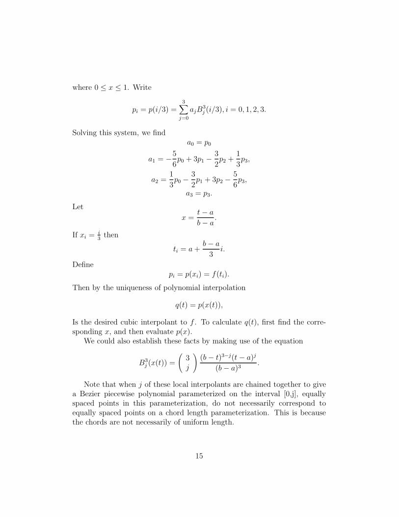
where 0 ≤ x ≤ 1. Write

pi = p(i/3) =3∑

j=0

ajB3j (i/3), i = 0, 1, 2, 3.

Solving this system, we finda0 = p0

a1 = −5

6p0 + 3p1 − 3

2p2 +

1

3p3,

a2 =1

3p0 − 3

2p1 + 3p2 − 5

6p3,

a3 = p3.

Let

x =t − a

b − a.

If xi = i3

then

ti = a +b − a

3i.

Definepi = p(xi) = f(ti).

Then by the uniqueness of polynomial interpolation

q(t) = p(x(t)),

Is the desired cubic interpolant to f . To calculate q(t), first find the corre-sponding x, and then evaluate p(x).

We could also establish these facts by making use of the equation

B3j (x(t)) =

(3j

)(b − t)3−j(t − a)j

(b − a)3.

Note that when j of these local interpolants are chained together to givea Bezier piecewise polynomial parameterized on the interval [0,j], equallyspaced points in this parameterization, do not necessarily correspond toequally spaced points on a chord length parameterization. This is becausethe chords are not necessarily of uniform length.

15

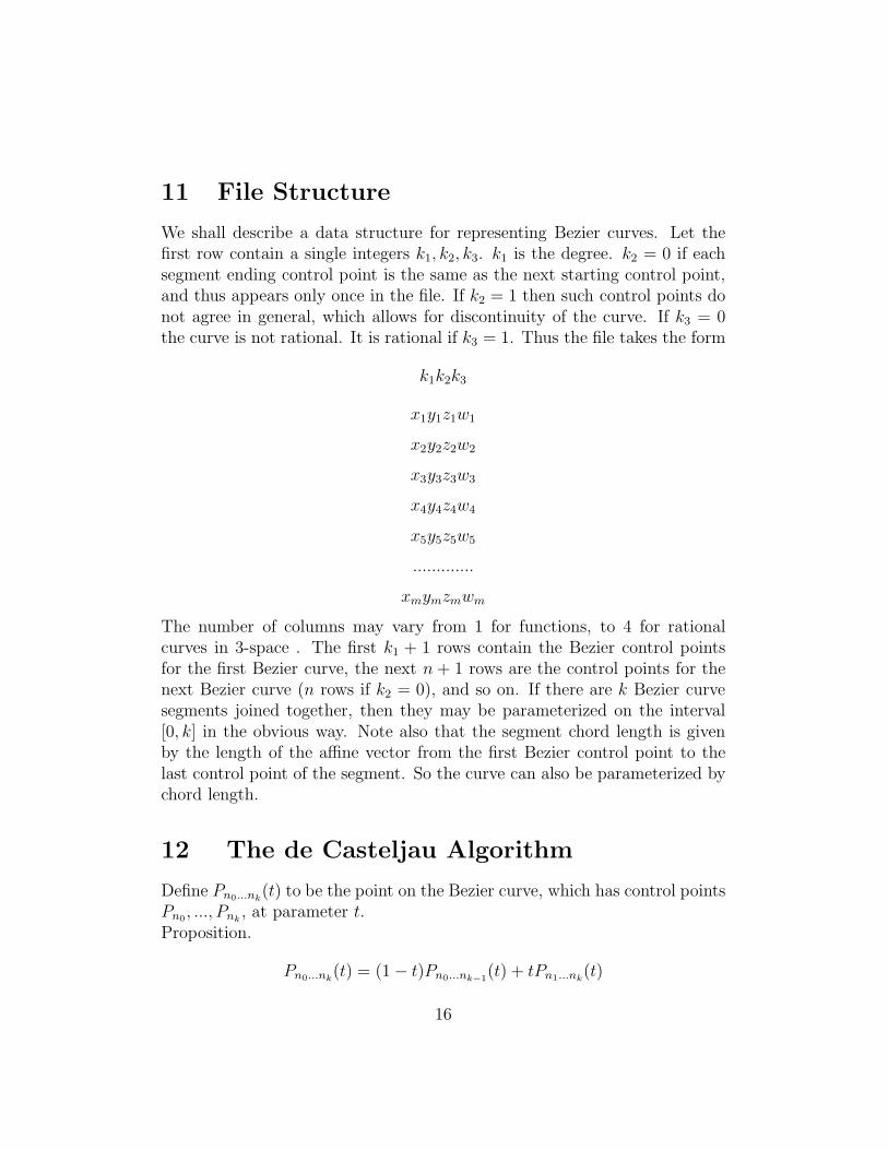
11 File Structure

We shall describe a data structure for representing Bezier curves. Let thefirst row contain a single integers k1, k2, k3. k1 is the degree. k2 = 0 if eachsegment ending control point is the same as the next starting control point,and thus appears only once in the file. If k2 = 1 then such control points donot agree in general, which allows for discontinuity of the curve. If k3 = 0the curve is not rational. It is rational if k3 = 1. Thus the file takes the form

k1k2k3

x1y1z1w1

x2y2z2w2

x3y3z3w3

x4y4z4w4

x5y5z5w5

.............

xmymzmwm

The number of columns may vary from 1 for functions, to 4 for rationalcurves in 3-space . The first k1 + 1 rows contain the Bezier control pointsfor the first Bezier curve, the next n + 1 rows are the control points for thenext Bezier curve (n rows if k2 = 0), and so on. If there are k Bezier curvesegments joined together, then they may be parameterized on the interval[0, k] in the obvious way. Note also that the segment chord length is givenby the length of the affine vector from the first Bezier control point to thelast control point of the segment. So the curve can also be parameterized bychord length.

12 The de Casteljau Algorithm

Define Pn0...nk(t) to be the point on the Bezier curve, which has control points

Pn0, ..., Pnk, at parameter t.

Proposition.

Pn0...nk(t) = (1 − t)Pn0...nk−1

(t) + tPn1...nk(t)

16

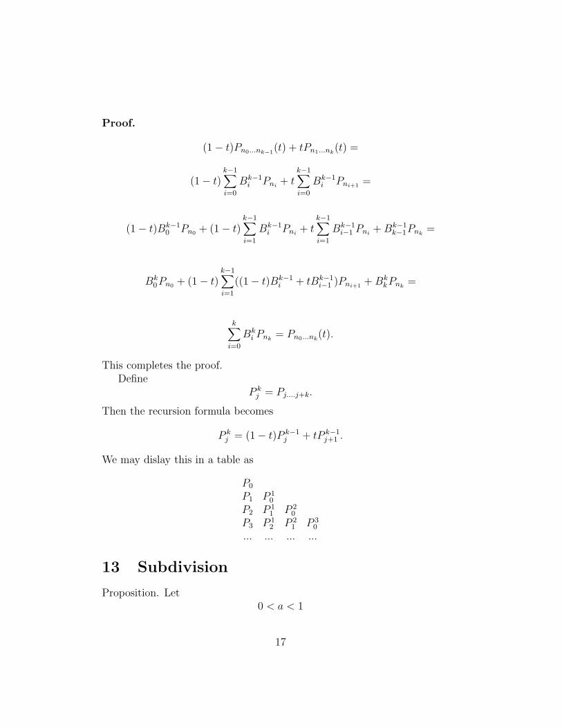
Proof.

(1 − t)Pn0...nk−1(t) + tPn1...nk

(t) =

(1 − t)k−1∑i=0

Bk−1i Pni

+ tk−1∑i=0

Bk−1i Pni+1

=

(1 − t)Bk−10 Pn0 + (1 − t)

k−1∑i=1

Bk−1i Pni

+ tk−1∑i=1

Bk−1i−1 Pni

+ Bk−1k−1Pnk

=

Bk0Pn0 + (1 − t)

k−1∑i=1

((1 − t)Bk−1i + tBk−1

i−1 )Pni+1+ Bk

kPnk=

k∑i=0

Bki Pnk

= Pn0...nk(t).

This completes the proof.Define

P kj = Pj....j+k.

Then the recursion formula becomes

P kj = (1 − t)P k−1

j + tP k−1j+1 .

We may dislay this in a table as

P0

P1 P 10

P2 P 11 P 2

0

P3 P 12 P 2

1 P 30

... ... ... ...

13 Subdivision

Proposition. Let0 < a < 1

17

then for t ∈ [0, 1]P0...k(at) = Q0...k(t),

whereQ0 = P0(a) = P0,

Q1 = P01(a),

Q2 = P012(a),

...........

Qk = P012..k(a).

Proof. Let k = 1 .Q01(t) = (1 − t)Q0 + tQ1 =

(1 − t)P0 + tP01(a) =

(1 − t)P0 + t((1 − a)P0 + aP1) =

(1 − ta)P0 + taP1 =

P01(at).

Proposition. Let0 < a < 1

then for t ∈ [0, 1]P0...k(a(1 − t) + t) = R0...k(t),

where

R0 = P0123...k(a).

........

Rk−2 = P(k−2)(k−1)k(a),

Rk−1 = P(k−1)k(a),

Rk = Pk(a) = P0,

Proof.

18

14 The WF-curve as a Bezier curve

The Wilson-Fowler curve (WF-curve) is an interpolating curve. Suppose itpasses through the interpolation points

P1, P2, ....., Pn.

Let ui be a unit vector in the direction of the ith line segment joining thepoints, that is in the direction of Pi+1 −Pi. Let vi be the unit vector rotateda positive 90 degrees from ui. These two vectors form a local coordinatesystem centered at Pi.

Let �i be the chord length of the ith segment and let si be the accumulatedchord length to the ith point. The the value c(s) of the Wilson-Fowler curveat a point on the ith segment, whose parameter s satisfies si ≤ s ≤ si+1, isgiven by

c(s) = Pi + (s − si)ui + fi(s − si)vi,

where

fi(x) =tai x(x − �i)

2 + tbix2(x − �i)

�2i

.

Note thatdfi(0)

dx= tai ,

anddfi(�i)

dx= tbi .

Consider

fi(x) =tai x(x − �i)

2 + tbix2(x − �i)

�2i

.

We shall find the Bezier control points for this curve and then translateand rotate to get the control points for the WF segment. For simplicity ofnotation we will suppress the i subscript with the understanding that we aredealing with the ith segment of the WF-curve.

Let w = x/�. Then f(x) = g(w) where

g(w) = �(ta + tb)w3 − (2ta + tb)w

2 + taw.

Multiplying the column vector of coefficients

19

�

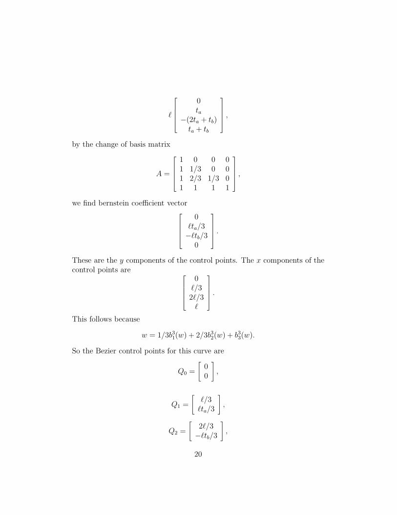
0ta

−(2ta + tb)ta + tb

,

by the change of basis matrix

A =

1 0 0 01 1/3 0 01 2/3 1/3 01 1 1 1

,

we find bernstein coefficient vector

0�ta/3−�tb/3

0

.

These are the y components of the control points. The x components of thecontrol points are

0

�/32�/3

�

.

This follows because

w = 1/3b31(w) + 2/3b3

2(w) + b33(w).

So the Bezier control points for this curve are

Q0 =

[00

],

Q1 =

[�/3

�ta/3

],

Q2 =

[2�/3−�tb/3

],

20

and

Q3 =

[�0

].

Now we shall rotate and translate the curve and thus rotate and translatethe control points, so that we obtain the ith WF curve segment. Define[

dx

dy

]= Pi+1 − Pi.

Then� =

√d2

x + d2y.

The proper rotation matrix is[dx/� −dy/�dy/� dx/�

].

After applying the rotation matrix we must translate by Pi. Thus the controlpoints for the ith WF segment are

Q0 = Pi,

Q1 = Pi +

[dx/3 − dyt

a/3dy/3 + dxt

a/3

],

Q2 = Pi +

[2dx/3 + dyt

b/32dy/3 − dxt

b/3

],

and

Q3 = Pi +

[dx

dy

]= Pi+1.

Therefore finally we have obtained a Bezier representation of the WF-curve.On the ith WF segment we have

c(s) = Q0b30(w) + Q1b

31(w) + Q2b

32(w) + Q3b

33(w),

where

0 ≤ w =s − si

�i≤ 1.

21

15 Barycentric Coordinates

Suppose we are given an n-simplex with vertices v0, v1, v2, ..., vn . The barycen-tric coordinates of a point p sum to one. If the coordinates satisfy

0 < λi < 1,

then the point is an interior point of the simplex. If any coordinate is nega-tive, then the point is exterior to the simplex. If

0 ≤ λi ≤ 1,

then the point is in the interior or on the boundary of the simplex. In thecase

0 ≤ λi ≤ 1,

when a coordinate λj = 0, the point is on the boundary of the simplexopposite the vertex pj .

To find the barycentric coordinates we may select an arbitrary vertex,say pn, and solve the linear system

n−1∑i=0

λi(pi − pn) = p − pn,

for λ0, ..., λn−1. Since the barycentric coordinates sum to 1, this also deter-mines λn.

Let us apply this to the problem of determining that a point is in atriangle of the plane. Suppose we are given the triangle vertices

p1 = (1, 2),

p2 = (1, 3),

p3 = (2, 3).

and wish to determine if p = (1.5, 2.6) is in the triangle. Our linear systemis [

(1 − 2) (1 − 2)(2 − 3) (3 − 3)

] [λ1

λ2

]=

[(1.5 − 2)(2.6 − 3)

].

The solution isλ1 = .1, λ2 = .4

22

Then we compute λ3 = .5. Therefore, because all coordinates are between 0and 1, the point is in the triangle.

The general computation to determine an interior point, requires 11 addi-tions or subtractions, 6 multiplications, 2 divisions, and 3 comparisons. Thecomputation may be done as follows.

Let a11 = x1 − x3,a21 = y1 − y3,a12 = x2 − x3,a22 = y2 − y3, and b1 =x − x3,b2 = y − y3. Then letting D be the determinant

D = a11a22 − a21a12,

we have

λ1 =b1a22 − b2a12

D,

λ2 =a11b2 − a21b1

D,

andλ3 = 1 − λ1 − λ2

23