Bezier Curve for Trajectory Guidance´

Bezier Curve for Trajectory Guidance

Ji-wung Choi ∗, Gabriel Hugh Elkaim †

Abstract—In this paper we present two path planningalgorithms based on Bezier curves for autonomous vehicleswith waypoints and corridor constraints. Bezier curves haveuseful properties for the path generation problem. The paperdescribes how the algorithms apply these properties to gen-erate the reference trajectory for vehicles to satisfy the pathconstraints. Both algorithms join cubic Bezier curve segmentssmoothly to generate the path. Additionally, we discuss theconstrained optimization problem that optimizes the resultingpath for user-defined cost function. The simulation shows thegeneration of successful routes for autonomous vehicles usingthese algorithms as well as control results for a simple kine-matic vehicle. Extensions of these algorithms towards navigat-ing through an unstructured environment with limited sensorrange are discussed.

Keywords: Bezier, Path Planning, Optimization, AutonomousVehicle, Feedback Control.

1. IntroductionExploiting the versatility of autonomous vehicles for aca-demic, industrial, and military applications will have a pro-found effect on future applications. Current research oncontrol systems for autonomous vehicles demonstrates thattrajectory generation is hardly a “solved” problem. For ve-hicle viability, it is imperative to be able to generate safepaths in real time.

Many path planning techniques for autonomous vehi-cles have been discussed in the literature. Cornell Uni-versity Team for 2005 DARPA Grand Challenge [8] useda path planner based on Bezier curves of degree 3 in a sens-ing/action feedback loop to generate smooth paths that areconsistent with vehicle dynamics. Skrjanc [7] proposed anew cooperative collision avoidance method for multiplerobots with constraints and known start and goal veloci-ties based on Bezier curves of degree 5. In this method,four control points out of five are placed such that desiredpositions and velocities of the start and the goal point aresatisfied. The fifth point is obtained by minimizing penaltyfunctions. Lizarraga [5] used Bezier curves for generating

∗Ph.D. Student, Autonomous Systems Lab, Computer Engineering De-partment, University of California, Santa Cruz, 95064, Tel: 831-428-2146,Email: [email protected]†Assistant Professor, Autonomous Systems Lab, Computer Engineer-

ing Department, University of California, Santa Cruz, 95064, Tel: 831-459-3054, Email: [email protected]

spatially deconflicted paths for multiple UAVs.Connors and Elkaim [1] previously presented a method

for developing feasible paths through complicated environ-ments using a kernel function based on cubic splines. Thismethod iteratively refines the path to compute a feasiblepath and thus find a collision free path in real time throughan unstructured environment. This method, when imple-mented in a receding horizon fashion, becomes the basisfor high level control. This previous method, however, re-sult in an incomplete path planning algorithm to satisfy thecomputational requirements in a complicated environment.A new approach has been developed based on using Beziercurves as the seed function for the path planning algorithmas an alternative to cubic splines. The resulting path is ma-nipulated by the control points of the bounding polygon.Though the optimization function for collision avoidanceis non-linear, it can be solved quickly and efficiently. Theresults of the new algorithm demonstrate the generation ofhigher performance, more efficient, and successful routesfor autonomous vehicles. Feedback control is used to trackthe planned path. The new algorithm is validated using sim-ulations, and demonstrates a successful tracking result of avehicle.

The paper is organized as follows: Section 2 begins bydescribing the definition of the Bezier curve and its usefulproperties for path planning. Section 3 discusses the con-trol problem for autonomous vehicles, the vehicle dynam-ics, and vehicle control algorithms. Section 4 proposes fourpath planning methods of which two are based on Beziercurves, and discusses the constrained optimization problemof these methods. In Section 5, simulation results of controlproblem for autonomous vehicles are given. Finally, Sec-tion 6 provides conclusions and future work.

2. Bezier CurveBezier Curves were invented in 1962 by the French engi-neer Pierre Bezier for designing automobile bodies. TodayBezier Curves are widely used in computer graphics and an-imation [6]. A Bezier Curve of degree n can be representedas

P[t0,t1](t) =n∑

i=0

Bni (t)Pi

Proceedings of the World Congress on Engineering and Computer Science 2008WCECS 2008, October 22 - 24, 2008, San Francisco, USA

ISBN: 978-988-98671-0-2 WCECS 2008

Where Pi are control points such that P (t0) = P0 andP (t1) = Pn, Bn

i (t) is a Bernstein polynomial given by

Bni (t) =

(ni

)(t1 − tt1 − t0

)n−i(t− t0t1 − t0

)i, i ∈ {0, 1, . . . , n}

Bezier Curves have useful properties for path planning:

• They always passes through P0 and Pn.

• They are always tangent to the lines connecting P0 →P1 and Pn → Pn−1 at P0 and Pn respectively.

• They always lie within the convex hull consisting oftheir control points.

2.1. The de Casteljau AlgorithmThe de Casteljau Algorithm is named after the French math-ematician Paul de Casteljau, who developed the algorithmin 1959. The de Casteljau algorithm describes a recursiveprocess to subdivide a Bezier curve P[t0,t2](t) into two seg-ments P[t0,t1](t) and P[t1,t2](t) [6]. Let {P 0

0 , P01 , . . . , P

0n}

denote the control points of P[t0,t2](t). The control pointsof P[t0,t1](t) and P[t1,t2](t) can be computed by

P ji =(1− τ)P j−1

i + τP j−1i+1 ,

j ∈ {1, . . . , n}, i ∈ {0, . . . , n− j}(1)

where τ = t1−t0t2−t0

. Then, {P 00 , P

10 , . . . , P

n0 } are the control

points of P[t0,t1] and {Pn0 , P

n1 − 1, . . . , P 0

n} are the controlpoints of P[t1,t2].

Remark 1. A Bezier curve P[t0,t2] always passes throughthe point P (t1) = Pn

0 computed by applying the de Castel-jau algorithm to subdivide itself into P[t0,t1] and P[t1,t2].

Also, it is always tangent to Pn−10 Pn−1

1 at P (t1).

The path planning method introduced in the Section4.3.2 is motivated by this property.

2.2. DerivativesThe derivatives of a Bezier curve, referred to as the hodo-graph, can be determined by its control points [6]. For aBezier curve P[t0,t1](t) =

∑ni=0B

ni (t)Pi, the first deriva-

tive can be represented as:

P[t0,t1](t) =n−1∑i=0

Bn−1i (t)Di (2)

Where Di, control points of P[t0,t1](t) is

Di =n

t1 − t0(Pi+1 − Pi)

The higher order derivative of a Bezier curve can be ob-tained by using the relationship of Equation (2).

2.3. CurvatureThe curvature of a n degree Bezier curve P[t0,t1] at its end-point is given by [6]

κ(t0) =n− 1n

h0

|P0 − P1|2(3)

κ(t1) =n− 1n

h1

|Pn−1 − Pn|2(4)

Where h0 is the distance from P2 to the line segment P0P1,h1 is the distance from PN−2 to the line segment Pn−1Pn.

3. Problem StatementConsider the control problem of a ground vehicle with amission defined by waypoints and corridor constraints ina two-dimensional free-space. Our goal is to develop andimplement an algorithm for navigation that satisfies theseconstraints. Let us denote each waypoint Wi ∈ R2 fori ∈ {1, 2, . . . , N}, where N ∈ R is the total number ofwaypoints. Corridor width is denoted as wj , j-th widths ofeach segment between two waypoints, j ∈ {1, . . . , N − 1}.

3.1. Dynamic Model of Vehicle MotionThis section describes a dynamic model for motion of avehicle that is used in the simulation in Section 5. Forthe dynamics of the vehicle, the state and the control vec-tor are denoted q(t) = (xc(t), yc(t), ψ(t))T and u(t) =(v(t), ω(t))T respectively. Where (xc, yc) represents theposition of the center of gravity of the vehicle. The vehi-cle yaw angle ψ is defined to the angle from the X axis.v is the longitudinal velocity of the vehicle at the center ofgravity. ω = ψ is the yaw angular velocity. It follows that

q(t) =

cosψ(t) 0sinψ(t) 0

0 1

u(t)

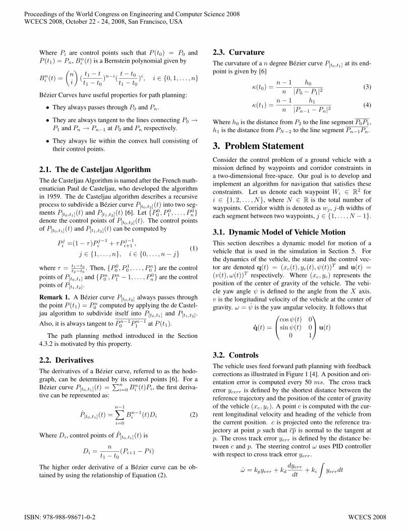
3.2. ControlsThe vehicle uses feed forward path planning with feedbackcorrections as illustrated in Figure 1 [4]. A position and ori-entation error is computed every 50 ms. The cross trackerror ycerr is defined by the shortest distance between thereference trajectory and the position of the center of gravityof the vehicle (xc, yc). A point c is computed with the cur-rent longitudinal velocity and heading of the vehicle fromthe current position. c is projected onto the reference tra-jectory at point p such that cp is normal to the tangent atp. The cross track error yerr is defined by the distance be-tween c and p. The steering control ω uses PID controllerwith respect to cross track error yerr.

ω = kpyerr + kddyerr

dt+ ki

∫yerrdt


ISBN: 978-988-98671-0-2 WCECS 2008

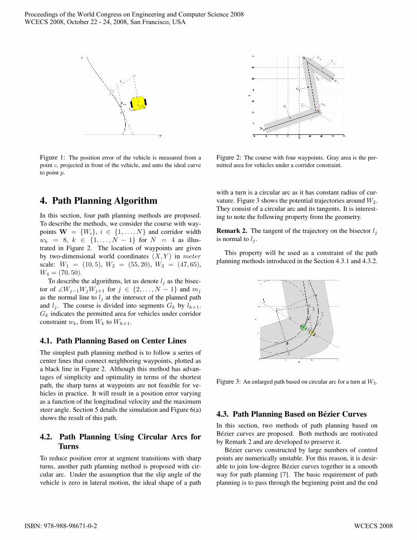
Figure 1: The position error of the vehicle is measured from apoint c, projected in front of the vehicle, and unto the ideal curveto point p.

4. Path Planning AlgorithmIn this section, four path planning methods are proposed.To describe the methods, we consider the course with way-points W = {Wi}, i ∈ {1, . . . , N} and corridor widthwk = 8, k ∈ {1, . . . , N − 1} for N = 4 as illus-trated in Figure 2. The location of waypoints are givenby two-dimensional world coordinates (X,Y ) in meterscale: W1 = (10, 5), W2 = (55, 20), W3 = (47, 65),W4 = (70, 50).

To describe the algorithms, let us denote lj as the bisec-tor of ∠Wj−1WjWj+1 for j ∈ {2, . . . , N − 1} and mj

as the normal line to lj at the intersect of the planned pathand lj . The course is divided into segments Gk by lk+1.Gk indicates the permitted area for vehicles under corridorconstraint wk, from Wk to Wk+1.

4.1. Path Planning Based on Center LinesThe simplest path planning method is to follow a series ofcenter lines that connect neighboring waypoints, plotted asa black line in Figure 2. Although this method has advan-tages of simplicity and optimality in terms of the shortestpath, the sharp turns at waypoints are not feasible for ve-hicles in practice. It will result in a position error varyingas a function of the longitudinal velocity and the maximumsteer angle. Section 5 details the simulation and Figure 6(a)shows the result of this path.

4.2. Path Planning Using Circular Arcs forTurns

To reduce position error at segment transitions with sharpturns, another path planning method is proposed with cir-cular arc. Under the assumption that the slip angle of thevehicle is zero in lateral motion, the ideal shape of a path

Figure 2: The course with four waypoints. Gray area is the per-mitted area for vehicles under a corridor constraint.

with a turn is a circular arc as it has constant radius of cur-vature. Figure 3 shows the potential trajectories aroundW2.They consist of a circular arc and its tangents. It is interest-ing to note the following property from the geometry.

Remark 2. The tangent of the trajectory on the bisector ljis normal to lj .

This property will be used as a constraint of the pathplanning methods introduced in the Section 4.3.1 and 4.3.2.

Figure 3: An enlarged path based on circular arc for a turn at W2.

4.3. Path Planning Based on Bezier CurvesIn this section, two methods of path planning based onBezier curves are proposed. Both methods are motivatedby Remark 2 and are developed to preserve it.

Bezier curves constructed by large numbers of controlpoints are numerically unstable. For this reason, it is desir-able to join low-degree Bezier curves together in a smoothway for path planning [7]. The basic requirement of pathplanning is to pass through the beginning point and the end


ISBN: 978-988-98671-0-2 WCECS 2008

point with different desired velocities. The least degree ofthe Bezier curve that can satisfy this requirement is three(See properties of Bezier curves in Section 2). Both meth-ods use a set of cubic Bezier curves.

The cubic Bezier curves used for the path planningare denoted as P[ti−1,ti](t) =

∑3k=0B

3k(t)Pk,i for i ∈

{1, . . . ,M} where M is the total number of the Beziercurves. The planned path P (t) for t ∈ [t0, tM ] is repre-sented as

P (t) = {P[ti−1,ti](t)}, i ∈ {1, . . . ,M}

4.3.1 Path Planning Placing Bezier Curves within Seg-ments

In this path planning method, the cubic Bezier curvesP[ti−1,ti](t) =

∑3k=0B

3k(t)Pk,i for i ∈ {1, . . . , N − 1}

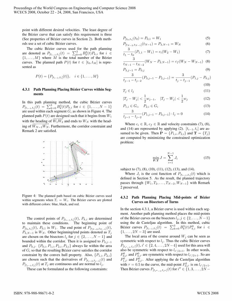
are used within each segment Gi as shown in Figure 4. Theplanned path P (t) are designed such that it begins from W1

with the heading of−−−−→W1W2 and ends to WN with the head-

ing of−−−−−−−→WN−1WN . Furthermore, the corridor constraint and

Remark 2 are satisfied.

Figure 4: The planned path based on cubic Bezier curves usedwithin segments when Ti = Wi. The Bezier curves are plottedwith different colors: blue, black, and red.

The control points of P[ti−1,ti](t), Pk,i are determinedto maintain these conditions. The beginning point ofP[t0,t1](t), P0,1 is W1. The end point of P[tN−2,tN−1](t),P3,N−1 is WN . Other beginning/end points denoted as Tj

are chosen on the bisectors lj for j ∈ {2, . . . , N − 1} andbounded within the corridor. Then it is assigned to P3,j−1

and P0,j . {P0,i, P1,i, P2,i, P3,i} always lie within the areaofGi so that the resulting Bezier curve satisfies the corridorconstraint by the convex hull property. Also, {P1,i, P2,i}are chosen such that the derivatives of P[tj−2,tj−1](t) andP[tj−1,tj ](t) at Tj are continuous and are normal to lj .

These can be formulated as the following constraints:

P[t0,t1](t0) = P0,1 = W1 (5)P[tN−2,tN−1](tN−1) = P3,N−1 = WN (6)

3t1 − t0

(P1,1 −W1) = ci(W2 −W1) (7)

3tN−1 − tN−2

(WN − P2,N−1) = cf (WN −WN−1) (8)

P3,j−1 = P0,j (9)3

tj−1 − tj−2(P3,j−1 − P2,j−1) =

3tj − tj−1

(P1,j − P0,j)

(10)

Tj ∈ lj (11)

|Tj −Wj | <12wj−1, |Tj −Wj | <

12wj (12)

P1,i ∈ Gi, P2,i ∈ Gi (13)3

tj−1 − tj−2(P1,j−1 − P0,j−1) · lj = 0 (14)

Where ci ∈ R, cf ∈ R and velocity constraints (7), (8),and (14) are represented by applying (2). [ti−1, ti] are as-sumed to be given. Then P = {P1,i, P2,i} and T = {Tj}are computed by minimizing the constrained optimizationproblem:

minP,T

J =N−1∑i=1

Ji (15)

subject to (7), (8), (10), (11), (12), (13), and (14).Where Ji is the cost function of P[ti−1,ti](t) which is

defined in Section 5. As the result, the planned trajectorypasses through {W1, T2, . . . , TN−2,WN−1} with Remark2 preserved.

4.3.2 Path Planning Placing Mid-points of BezierCurves on Bisectors of Turns

In the section 4.3.1, a Bezier curve is used within each seg-ment. Another path planning method places the mid-pointsof the Bezier curves on the bisectors lj , j ∈ {2, . . . , N −1}using the de Casteljau algorithm. In this method, cubicBezier curves P[ti−1,ti](t) =

∑3k=0B

3k(t)P 0

k,i for i ∈{1, . . . , 2N − 3} are used.

The local area of the course around Wj can be seen assymmetric with respect to lj . Thus the cubic Bezier curvesP[ti′−1,ti′ ]

(t), i′ ∈ {2, 4, . . . , 2N−4} used for this area willalso be symmetric with respect to li′/2+1. In other words,P 0

0,i′ and P 03,i′ are symmetric with respect to li′/2+1. So are

P 01,i′ and P 0

2,i′ . After applying the de Casteljau algorithmwith τ = 0.5 to the curve, the mid-point P 3

0,i′ is on li′/2+1.Then Bezier curves P[ti′′−1,ti′′ ]

(t) for i′′ ∈ {1, 3, . . . , 2N−


ISBN: 978-988-98671-0-2 WCECS 2008

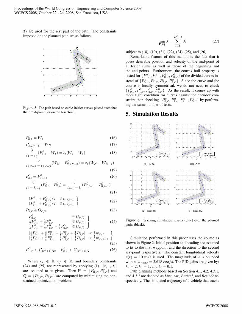
3} are used for the rest part of the path. The constraintsimposed on the planned path are as follows:

Figure 5: The path based on cubic Bezier curves placed such thattheir mid-point lies on the bisectors.

P 00,1 = W1 (16)

P 03,2N−3 = WN (17)3

t1 − t0(P 0

1,1 −W1) = ci(W2 −W1) (18)

3t2N−4 − t2N−3

(WN − P 02,2N−3) = cf (WN −WN−1)

(19)

P 03,i = P 0

0,i+1 (20)3

ti − ti−1(P 0

3,i − P 02,i) =

3ti+1 − ti

(P 01,i+1 − P 0

0,i+1)

(21)

(P 00,i′ + P 0

3,i′)/2 ∈ li′/2+1

(P 01,i′ + P 0

2,i′)/2 ∈ li′/2+1

}(22)

P 03,i′ ∈ Gi′/2 (23)

P 00,i′ ∈ Gi′/2

12P

00,i′ +

12P

01,i′ ∈ Gi′/2

14P

00,i′ +

12P

01,i′ +

14P

02,i′ ∈ Gi′/2

(24)

| 18P00,i′ +

38P

01,i′ +

38P

02,i′ +

18P

03,i′ | < 1

2wi′/2

| 18P00,i′ +

38P

01,i′ +

38P

02,i′ +

18P

03,i′ | < 1

2wi′/2+1

}(25)

P 01,i′′ ∈ G(i′′+1)/2, P 0

2,i′′ ∈ G(i′′+1)/2 (26)

Where ci ∈ R, cf ∈ R, and boundary constraints(24) and (25) are represented by applying (1). [ti−1, ti]are assumed to be given. Then P = {P 0

0,i′ , P01,i′} and

Q = {P 01,i′′ , P

02,i′′} are computed by minimizing the con-

strained optimization problem:

minP,Q

J =2N−3∑i=1

Ji (27)

subject to (18), (19), (21), (22), (24), (25), and (26).Remarkable feature of this method is the fact that it

poses desirable position and velocity of the mid-point ofa Bezier curve as well as those of the beginning andthe end points. Furthermore, the convex hull property istested for {P 0

0,i′ , P10,i′ , P

20,i′ , P

30,i′} of the divided curves in-

stead of {P 00,i′ , P

01,i′ , P

02,i′ , P

03,i′}. Since the curve and the

course is locally symmetrical, we do not need to check{P 3

0,i′ , P21,i′ , P

12,i′ , P

03,i′}. As the result, it comes up with

more tight condition for curves against the corridor con-straint than checking {P 0

0,i′ , P01,i′ , P

02,i′ , P

03,i′} by perform-

ing the same number of tests.

5. Simulation Results

(a) Line (b) Arc

(c) Bezier1 (d) Bezier2

Figure 6: Tracking simulation results (blue) over the plannedpaths (black).

Simulation performed in this paper uses the course asshown in Figure 2. Initial position and heading are assumedto fit to the first waypoint and the direction to the secondwaypoint respectively. The constant longitudinal velocityv(t) = 10 m/s is used. The magnitude of ω is boundedwithin |ω|max = 2.618 rad/s. The PID gains are given by:kp = 2, kd = 1, and ki = 0.1.

Path planning methods based on Section 4.1, 4.2, 4.3.1,and 4.3.2 are denoted as Line, Arc, Bezier1, and Bezier2 re-spectively. The simulated trajectory of a vehicle that tracks


ISBN: 978-988-98671-0-2 WCECS 2008

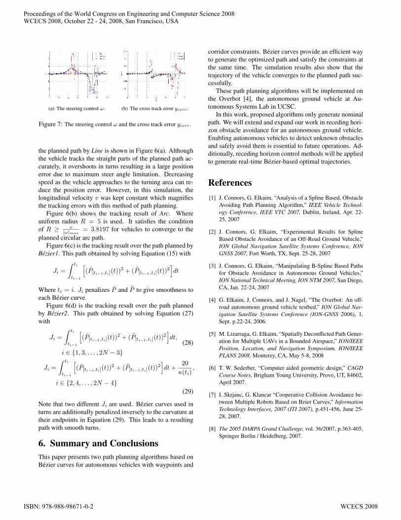
(a) The steering control ω. (b) The cross track error ycerr .

Figure 7: The steering control ω and the cross track error ycerr .

the planned path by Line is shown in Figure 6(a). Althoughthe vehicle tracks the straight parts of the planned path ac-curately, it overshoots in turns resulting in a large positionerror due to maximum steer angle limitation. Decreasingspeed as the vehicle approaches to the turning area can re-duce the position error. However, in this simulation, thelongitudinal velocity v was kept constant which magnifiesthe tracking errors with this method of path planning.

Figure 6(b) shows the tracking result of Arc. Whereuniform radius R = 5 is used. It satisfies the conditionof R ≥ v

|ω|max= 3.8197 for vehicles to converge to the

planned circular arc path.Figure 6(c) is the tracking result over the path planned by

Bezier1. This path obtained by solving Equation (15) with

Ji =∫ ti

ti−1

[(P[ti−1,ti](t))

2 + (P[ti−1,ti](t))2]dt

Where ti = i. Ji penalizes P and P to give smoothness toeach Bezier curve.

Figure 6(d) is the tracking result over the path plannedby Bezier2. This path obtained by solving Equation (27)with

Ji =∫ ti

ti−1

[(P[ti−1,ti](t))

2 + (P[ti−1,ti](t))2]dt,

i ∈ {1, 3, . . . , 2N − 3}(28)

Ji =∫ ti

ti−1

[(P[ti−1,ti](t))

2 + (P[ti−1,ti](t))2]dt+

20κ(ti)

,

i ∈ {2, 4, . . . , 2N − 4}(29)

Note that two different Ji are used. Bezier curves used inturns are additionally penalized inversely to the curvature attheir endpoints in Equation (29). This leads to a resultingpath with smooth turns.

6. Summary and ConclusionsThis paper presents two path planning algorithms based onBezier curves for autonomous vehicles with waypoints and

corridor constraints. Bezier curves provide an efficient wayto generate the optimized path and satisfy the constraints atthe same time. The simulation results also show that thetrajectory of the vehicle converges to the planned path suc-cessfully.

These path planning algorithms will be implemented onthe Overbot [4], the autonomous ground vehicle at Au-tonomous Systems Lab in UCSC.

In this work, proposed algorithms only generate nominalpath. We will extend and expand our work in receding hori-zon obstacle avoidance for an autonomous ground vehicle.Enabling autonomous vehicles to detect unknown obstaclesand safely avoid them is essential to future operations. Ad-ditionally, receding horizon control methods will be appliedto generate real-time Bezier-based optimal trajectories.

References[1] J. Connors, G. Elkaim, “Analysis of a Spline Based, Obstacle

Avoiding Path Planning Algorithm,” IEEE Vehicle Technol-ogy Conference, IEEE VTC 2007, Dublin, Ireland, Apr. 22-25, 2007

[2] J. Connors, G. Elkaim, “Experimental Results for SplineBased Obstacle Avoidance of an Off-Road Ground Vehicle,”ION Global Navigation Satellite Systems Conference, IONGNSS 2007, Fort Worth, TX, Sept. 25-28, 2007

[3] J. Connors, G. Elkaim, “Manipulating B-Spline Based Pathsfor Obstacle Avoidance in Autonomous Ground Vehicles,”ION National Technical Meeting, ION NTM 2007, San Diego,CA, Jan. 22-24, 2007

[4] G. Elkaim, J. Connors, and J. Nagel, “The Overbot: An off-road autonomous ground vehicle testbed,” ION Global Nav-igation Satellite Systems Conference (ION-GNSS 2006), 1,Sept. p.22-24, 2006.

[5] M. Lizarraga, G. Elkaim, “Spatially Deconflicted Path Gener-ation for Multiple UAVs in a Bounded Airspace,” ION/IEEEPosition, Location, and Navigation Symposium, ION/IEEEPLANS 2008, Monterey, CA, May 5-8, 2008

[6] T. W. Sederber, “Computer aided geometric design,” CAGDCourse Notes, Brigham Young University, Provo, UT, 84602,April 2007.

[7] I. Skrjanc, G. Klancar “Cooperative Collision Avoidance be-tween Multiple Robots Based on Bzier Curves,” InformationTechnology Interfaces, 2007 (ITI 2007), p.451-456, June 25-28, 2007.

[8] The 2005 DARPA Grand Challenge, vol. 36/2007, p.363-405,Springer Berlin / Heidelberg, 2007.


ISBN: 978-988-98671-0-2 WCECS 2008

Documents

Bezier Curve for Trajectory Guidance´