Beyond Uniformity and Independence : Analysis of R-trees Usingthe Concept of Fractal DimensionChristos Faloutsos� and Ibrahim KamelDepartment of Computer Science andInstitute for Systems Research (ISR)Univ. of Maryland at College ParkFebruary 24, 1994AbstractWe propose the concept of fractal dimension of a set of points, in order to quantify thedeviation from the uniformity distribution. Using measurements on real data sets (road inter-sections of U.S. counties, star coordinates from NASA's Infrared-Ultraviolet Explorer etc.) weprovide evidence that real data indeed are skewed, and, moreover, we show that they behave asmathematical fractals, with a measurable, non-integer fractal dimension.Armed with this tool, we then show its practical use in predicting the performance of spatialaccess methods, and speci�cally of the R-trees. We provide the �rst analysis of R-trees forskewed distributions of points: We develop a formula that estimates the number of disk accessesfor range queries, given only the fractal dimension of the point set, and its count. Experimentson real data sets show that the formula is very accurate: the relative error is usually below 5%,and it rarely exceeds 10%.We believe that the fractal dimension will help replace the uniformity and independenceassumptions, allowing more accurate analysis for any spatial access method, as well as betterestimates for query optimization on multi-attribute queries.1 IntroductionIn this work we study the distribution of real datasets with D-dimensional points. Sets of multi-dimensional points appear in several database applications: records in relational DBMSs can be�This research was partially funded by the National Science Foundation under Grants IRI-9205273 and IRI-8958546(PYI), with matching funds from EMPRESS Software Inc. and Thinking Machines Inc.1

viewed as points in attribute space; geographic information systems (GIS) [21] contain point data,such as cities on a 2-dimensional map; medical image databases with, eg., 3-dimensional MRI brainscans, require the storage and retrieval of point-sets, such as digitized surfaces of brain structures [2],etc. For the balance of this work, the term point-set and dataset will be used interchangeably.An interesting problem is the estimation of the search e�ort for range queries, when thepoints are stored in a spatial access method (SAM), such as an R-tree. A closely related problemis the estimation of selectivity (ie., number of qualifying points) for range queries: this is usefulin the query optimization in an RDBMS with multidimensional queries [14] or in a GIS [1]. Thetraditional assumptions are the uniformity and independence assumption, which make the analysistractable.However, these assumptions do not hold on real data; moreover, they lead to pessimisticestimates [5]. For a single attribute, the uniformity assumption has been relaxed, eg., [10], typicallyusing the Zipf distribution [24]. Distributions of real attributes indeed follow the Zipf distributionor the generalized Zipf distribution: for example, word frequencies in the English language (as wellas other languages); salaries [24]; �rst names and last names of people [7], etc.However, no attempt has been made to model multi-dimensional distributions. Theoreticalanalyses in such cases assume that points are uniformly distributed in the address space [6],[1],which also implies that the attributes are uncorrelated. Even in simulation studies, researcherson spatial access methods and multi-attribute query optimization are forced to use ad-hoc, non-uniform distributions, such as the gaussian distribution [15], some sort of clustered distributions(with points clustering around uniformly distributed sites [17], or points clustering around curves,like the sinusoidal curve [4]), or even to obey the independence assumption anyway [14]. Althoughnon-uniform, it is unclear whether these distributions resemble real distributions.Evidence that real distributions violate both assumptions is overwhelming. Figure 1 providesa counter-example for both assumptions, using two real datasets. Figure 1(a) shows the populationvs. area scatter-plot for 181 nations, from the World Factbook (available, eg., with anonymousftp from ocf.berkeley.edu, /ftp/pub/Library/Reference/World Factbook). Notice that thepoints follow a highly skewed distribution: there are a few large and/or highly populated nations(eg., China, India), while the vast majority of points is close to the origin. Figure 1(b) shows thesame scatter plot in doubly logarithmic scales, to highlight the strong correlation between area andpopulation.Figure 1 (c) shows the road intersections for the Montgomery County of Maryland. Noticethat the distribution is clearly non-uniform. Also notice that it does not resemble a gaussiandistribution either : there are several high-concentration areas (one for each city, like Bethesda,Rockville, Gaithersburg etc). 2

Population x 109

6Area x 10

0.00

0.10

0.20

0.30

0.40

0.50

0.60

0.70

0.80

0.90

1.00

1.10

1.20

0.00 2.00 4.00 6.00 8.00

Population

Area5

1e+04

2

5

1e+05

2

5

1e+06

2

5

1e+07

2

5

1e+08

2

5

1e+09

2

1e+01 1e+02 1e+03 1e+04 1e+05 1e+06 1e+07

x 103

3 x 10

0.00

2.00

4.00

6.00

8.00

10.00

12.00

14.00

16.00

18.00

20.00

22.00

24.00

26.00

28.00

30.00

0.00 5.00 10.00 15.00 20.00 25.00 30.00(a) (b) (c)Figure 1: (a) WORLD dataset (b) WORLD dataset - log-log scale (c) Cross-roads of MontgomeryCounty of MarylandIn conclusion, we need a way to describe distributions of real multi-dimensional points. Theproblem we want to solve is the following:GIVEN real distributions of multi-dimensional pointsFIND a way to characterize their deviation from uniformityTO PREDICT the search performance of a spatial access method (SAM).The description should allow us to analyze several types of queries, such as 'range' queries, 'nearestneighbor' queries, 'spatial joins' etc. In this paper we focus on range queries.For the above problem, we propose the concept of fractal dimension as the solution. We showthat several real distributions indeed exhibit fractal behavior, that is, they are self-similar: portionsof the point-set are statistically similar to the whole set (see Figure 3 for an example). We describehow to compute the fractal dimension of a set of points, and then we show how to use it to predictthe performance of spatial access methods that store this point-set. Speci�cally, we examine theR-trees and provide the �rst known analysis for them, for real distributions.The paper is organized as follows: Section 2 provides the background information aboutR-trees. Section 3 gives the de�nition of the fractal dimension, along with examples from realdata. Section 4 presents the analysis. Section 5 gives the experimental results and Section 6 liststhe conclusions. 3

2 BackgroundIn this section, we provide a brief description of R-trees [9], which will be the SAM that we use toillustrate our analysis. Additional SAMs include the quad-tree based methods [8, 17] and grid �leand its variants [16]; see [20] for a survey. We focus on the R-tree because it seems to be one ofthe most successful methods.The original R-tree [9] was suggested by Guttman; it is the extension of the B-tree formultidimensional objects. A geometric object is represented by its minimum bounding rectangle(MBR). Non-leaf nodes contain entries of the form (ptr,R) where ptr is a pointer to a child node inthe R-tree; R is the MBR that covers all rectangles in the child node. Leaf nodes contain entriesof the form (obj-id, R) where obj-id is a pointer to the object description, and R is the MBR ofthe object. The main innovation in the R-tree is that father nodes are allowed to overlap. Thisway, the R-tree can guarantee at least 50% space utilization and at the same time remain balanced.Figure 2 illustrates data rectangles (in black), organized in an R-tree with fanout 3.0 1

0

1

45

6

78

9

10

11 12

1

2

3Figure 2: Data (dark rectangles) organized in an R-tree with fanout=3Subsequent work on R-trees includes the packed- [19] and Hilbert-packed R-trees [12], theR+-tree [23], R-trees using Minimum Bounding Polygons [11] and the R�-tree [4]. The latter seemsto give the best search times, mainly thanks to the idea of deferring the splits by 'force-reinserting'some of the entries of the over owing nodes.The last part in this section is a summary of previous attempts to analyze the R-trees. In [6]we assumed that the points are uniformly distributed in the address space. Recently, we providedformulas [12] that assume that the R-tree has been built and that we can measure the MBR ofeach node of the R-tree. The results are as follows. Consider the n-th node of the tree, and let itsMBR be x1;n � : : :� xD;n. We denote it compactly as:~xn = (x1;n; : : : ; xD;n) (1)4

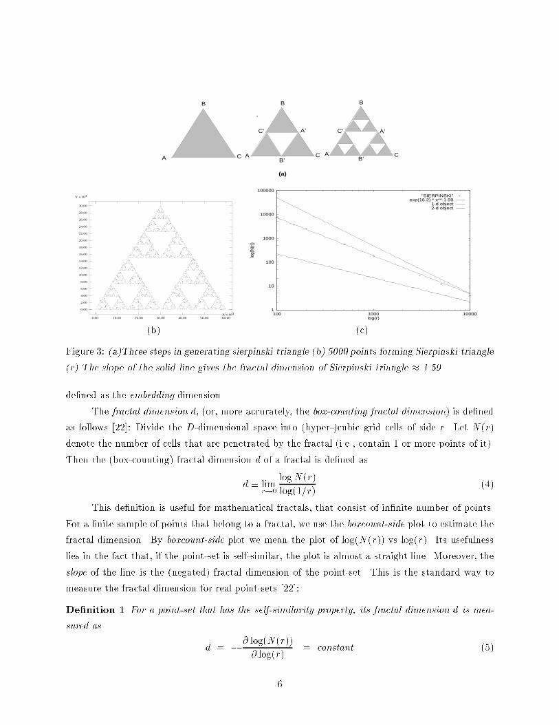
Similarly, let ~q = (q1; : : : ; qD) (2)denote a range query with side qi on the i-th dimension. Then, we have the following theorem:Theorem 1 The average number P (~q) of nodes (� pages) accessed by a query of sides ~q is givenby P (~q) =Xn DYi=1(xi;n + qi) (3)where the summation extends over all the nodes of the tree.Proof: See [12].A similar analysis, mainly focusing on square queries, was published independently in [18].Notice that Theorem 1 allows us to calculate the node accesses for any level of the tree: we onlyneed to restrict the summation over the nodes of the level(s) of interest.In the next sections we shall see how to predict the size of the MBRs of the nodes of the tree,before even the tree is built. To do that, we show that we only need the fractal dimension d of thepoint-set, and, of course, the number of points N and the fanout of the tree.3 Fractal DimensionIntuitively, a set of points is a fractal if it exhibits self-similarity over all scales. This is illustrated byan example: Figure 3(a) shows the �rst few steps in constructing the so-called Sierpinski triangle.Figure 3(b) gives 5,000 points that belong to this triangle. Theoretically, the Sierpinski triangle isderived from an equilateral triangle ABC, by excluding its middle (triangle A'B'C') and recursivelyrepeating this procedure for each of the resulting smaller triangles. The resulting set of pointsexhibits `holes' in any scale; moreover, each smaller triangle is a miniature replica of the wholetriangle. In general, the characteristic of fractals is this self-similarity property: parts of the fractalare similar (exactly or statistically) to the whole fractal. For our experiments we use 50,000 samplepoints from the Sierpinski triangle (`SIERPINSKI' dataset).The Sierpinski triangle gives an example of points which follow a highly non-uniform dis-tribution; yet, the distribution is deterministic, and easy to describe, at least in English. Thereshould be an equally easy, way to describe it mathematically.3.1 Formal de�nitions and MeasurementsConsider a geometrical object (eg., like the Sierpinski triangle) with the 'self-similarity' property,consisting of a set of points in D-dimensional space. The dimensionality D of the address space is5

B

CA A C

B

A C

B

C’

’

A’

B’

C’

B’

A’

(a)

Y x 103

3X x 10

0.00

2.00

4.00

6.00

8.00

10.00

12.00

14.00

16.00

18.00

20.00

22.00

24.00

26.00

28.00

30.00

0.00 10.00 20.00 30.00 40.00 50.00 60.00

1

10

100

1000

10000

100000

100 1000 10000

log(

N(r)

)

log(r)

"SIERPINSKI"exp(16.2) * x**-1.59

1-d object2-d object

(b) (c)Figure 3: (a)Three steps in generating sierpinski triangle (b) 5000 points forming Sierpinski triangle(c) The slope of the solid line gives the fractal dimension of Sierpinski triangle � 1.59de�ned as the embedding dimension.The fractal dimension d, (or, more accurately, the box-counting fractal dimension) is de�nedas follows [22]: Divide the D-dimensional space into (hyper-)cubic grid cells of side r. Let N(r)denote the number of cells that are penetrated by the fractal (i.e., contain 1 or more points of it).Then the (box-counting) fractal dimension d of a fractal is de�ned asd � limr!0 logN(r)log(1=r) (4)This de�nition is useful for mathematical fractals, that consist of in�nite number of points.For a �nite sample of points that belong to a fractal, we use the boxcount-side plot to estimate thefractal dimension. By boxcount-side plot we mean the plot of log(N(r)) vs log(r). Its usefulnesslies in the fact that, if the point-set is self-similar, the plot is almost a straight line. Moreover, theslope of the line is the (negated) fractal dimension of the point-set. This is the standard way tomeasure the fractal dimension for real point-sets [22]:De�nition 1 For a point-set that has the self-similarity property, its fractal dimension d is mea-sured as d = � @ log(N(r))@ log(r) = constant (5)6

Corollary 1 For a point-set with the self-similarity property, we haveN(r) = K=rd (6)where K is an integration constant.Proof: Since d remains constant with r, we obtain Eq. 6 by integrating Eq. 5.Next we give some examples to illustrate how the method works.(b)

(1,1)

(0,0)(a)(0,0)

(1,1)

r = 1/4 r = 1/8

(1,0)

(0,1) (0,1)

(1,0)Figure 4: Computing the fractal dimension of a line segmentExample 1: Figure 4 illustrates the method when the object is the diagonal line segment (0,0)-(1,1). Figure 4(a) shows that the line segment penetrates 4 boxes of side r = 1=4, and Figure 4(b)shows it penetrating 8 boxes of side r = 1=8. Thus, we haveN(r) = (1=r) = (1=r)1 r � 1 (7)and, therefore, d = �@ log((1=r)1)@ log(r) = 1 (8)which is intuitively expected, since a line segment is a 1-dimensional object.The fact that the fractal dimension of a line segment reduces to its Euclidean dimension isnot a coincidence: Notice that Euclidean objects, like lines, circles, planes etc. trivially ful�ll theself-similarity requirement: for example, a part of a line segment is a miniature replica of the wholesegment. Based on the above, we have [13]:Observation 1 For Euclidean objects, their fractal dimension reduces to their Euclidean dimen-sion.Thus, lines, line segments, circles, and all the standard curves have d=1; planes, disks and standardsurfaces have d=2; euclidian volumes in D-dimensional space have d = D.7

Example 2. This is an example of a fractal with a non-integer d. Figure 3-(c) shows the boxcount-side plot for the SIERPINSKI set of points of Figure 3-(b) The line has slope (-)1.59, while thetheoretical number is log 3= log 2 = 1.5849 [13]. The plot also contains two lines. The former corre-sponds to a 2-dimensional object (like unit square) and the latter corresponds, to a 1-dimensionalobject, such as the line segment of example 1, with slopes -2 and -1 respectively.3.2 Fractal dimensions of real datasetsIn the above examples, all the involved point-sets are known to have the self-similarity property,and therefore it is expected that their boxcount-side plots will be straight lines. The question iswhether real datasets exhibit self-similarity. Table 1 shows the characteristics of the datasets weused: The `MGCounty' and `LBCounty' datasets are part of the TIGER database of the US Bureauof Census and they contain the road intersections of the Montgomery county, MD and Long Beachcounty, CA, respectively. The `IUE' contains observation points (latitude and longitude of stars)from the International Ultraviolet Explorer (IUE) satellite of NASA. The WORLD dataset hasbeen discussed in the introduction (see Figure 1).In the upcoming plots we also used synthetic datasets: In addition to the SIERPINSKI onethat we have discussed we also used the 2D-UNIFORM, 1D-Uniform point sets. As their namesreveal, they consisted of points uniformly distributed in the unit square and on a line, respectivelyFigure 5 (a)-(d) shows the boxcount-side plots for all these datasets. Notice that the plotsare indeed straight lines, con�rming that real point-sets exhibit fractal behavior. This implies thatwe can use Eq. 6 to do useful predictions, as we show next. In all of �gures 5 (a)-(d) we also givethe boxcount-side plot for the two uniform synthetic datasets, 2D-UNIFORM and 1D-UNIFORM.The reason is that we want to highlight the fact that the slopes for the real sets are non-integers.This means that the real datasets are self similar, but clearly non-uniform.The conclusion is that we have con�rmed once more that real data sets are far from uniformlydistributed - the only di�erence is that, this time, we have a usable measure of their skewness!Before we continue with the analysis, we list a few more observations:Observation 2 The fractal dimension can model point-sets with highly correlated attributes, evenif the correlation is non-linear.The reason is that, if two attributes are strongly correlated (even in a quadratic, logarithmic orsome other non-linear fashion), the resulting set of points in attribute space will be a curve, withd=1, as we just discussed in Observation 1. The input point-set will be correctly characterized asa linear object, as opposed to a 2-dimensional object.8

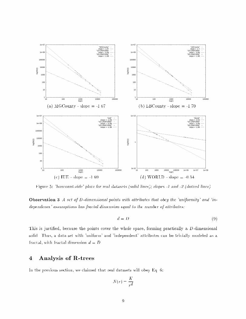
1

10

100

1000

10000

100000

1e+06

1e+07

10 100 1000 10000 100000

log(

N(r

))

log(r)

"MGCounty"slope = -1.67

"1D-UNIFORM"slope = -0.99

"2D-UNIFORM"slope = -1.98

1

10

100

1000

10000

100000

1e+06

1e+07

10 100 1000 10000 100000

log(

N(r

))

log(r)

"LBCounty"slope = -1.7

"1D-UNIFORM"slope = -0.99

"2D-UNIFORM"slope = -1.98

(a) MGCounty - slope = -1.67 (b) LBCounty - slope = -1.701

10

100

1000

10000

100000

1e+06

1e+07

10 100 1000 10000 100000

log(

N(r

))

log(r)

"IUE"slope = -1.69

"1D-UNIFORM"slope = -0.99

"2D-UNIFORM"slope = -1.98

1e-10

1

1e+10

10 100 1000 10000 100000 1e+06 1e+07 1e+08

log(

N(r

))

log(r)

"World"slope = -0.54

"1D-UNIFORM"slope = -0.99

"2D-UNIFORM"slope = -1.98

(c) IUE - slope = -1.69 (d) WORLD - slope = -0.54Figure 5: 'boxcount-side' plots for real datasets (solid lines); slopes -1 and -2 (dotted lines)Observation 3 A set of D-dimensional points with attributes that obey the 'uniformity' and 'in-dependence' assumptions has fractal dimension equal to the number of attributes:d = D (9)This is justi�ed, because the points cover the whole space, forming practically a D-dimensionalsolid. Thus, a data set with 'uniform' and 'independent' attributes can be trivially modeled as afractal, with fractal dimension d = D.4 Analysis of R-treesIn the previous section, we claimed that real datasets will obey Eq. 6:N(r) = Krd9

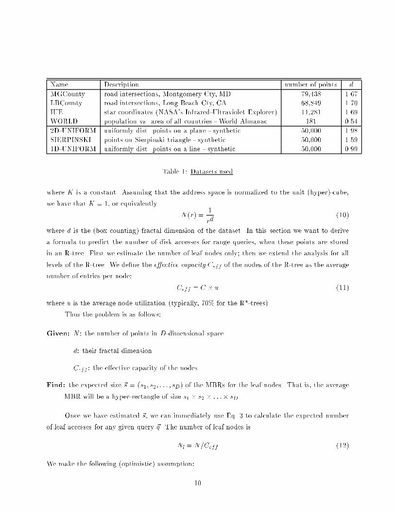
Name Description number of points dMGCounty road intersections, Montgomery Cty, MD 79,438 1.67LBCounty road intersections, Long Beach Cty, CA 68,849 1.70IUE star coordinates (NASA's Infrared-Ultraviolet Explorer) 11,281 1.69WORLD population vs. area of all countries - World Almanac 181 0.542D-UNIFORM uniformly dist. points on a plane - synthetic 50,000 1.98SIERPINSKI points on Sierpinski triangle - synthetic 50,000 1.591D-UNIFORM uniformly dist. points on a line - synthetic 50,000 0.99Table 1: Datasets usedwhere K is a constant. Assuming that the address space is normalized to the unit (hyper)-cube,we have that K = 1, or equivalently N(r) = 1rd (10)where d is the (box counting) fractal dimension of the dataset. In this section we want to derivea formula to predict the number of disk accesses for range queries, when these points are storedin an R-tree. First we estimate the number of leaf nodes only; then we extend the analysis for alllevels of the R-tree. We de�ne the e�ective capacity Ceff of the nodes of the R-tree as the averagenumber of entries per node: Ceff = C � u (11)where u is the average node utilization (typically, 70% for the R*-trees).Thus the problem is as follows:Given: N : the number of points in D-dimensional spaced: their fractal dimensionCeff : the e�ective capacity of the nodesFind: the expected size ~s = (s1; s2; : : : ; sD) of the MBRs for the leaf nodes. That is, the averageMBR will be a hyper-rectangle of size s1 � s2 � : : :� sDOnce we have estimated ~s, we can immediately use Eq. 3 to calculate the expected numberof leaf accesses for any given query ~q. The number of leaf nodes isNl = N=Ceff (12)We make the following (optimistic) assumption:10

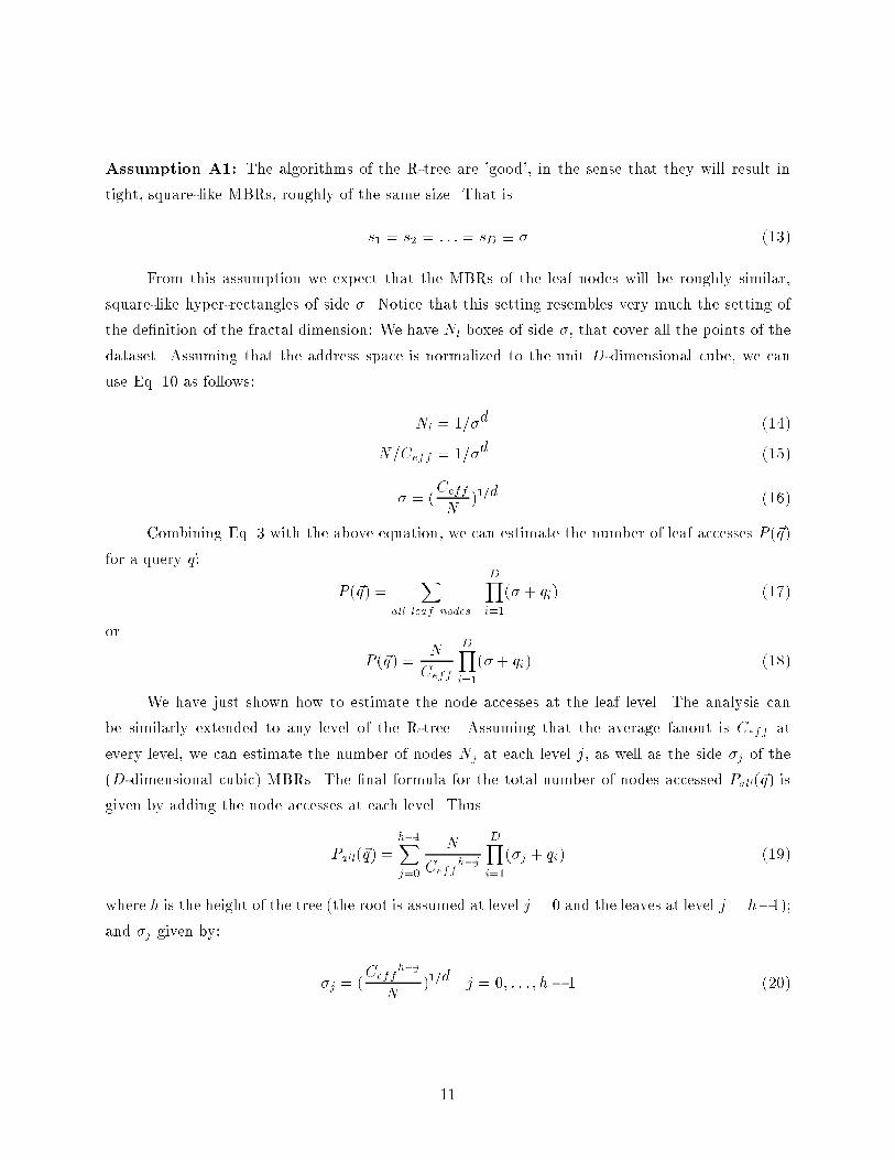
Assumption A1: The algorithms of the R-tree are 'good', in the sense that they will result intight, square-like MBRs, roughly of the same size. That iss1 = s2 = : : : = sD � � (13)From this assumption we expect that the MBRs of the leaf nodes will be roughly similar,square-like hyper-rectangles of side �. Notice that this setting resembles very much the setting ofthe de�nition of the fractal dimension: We have Nl boxes of side �, that cover all the points of thedataset. Assuming that the address space is normalized to the unit D-dimensional cube, we canuse Eq. 10 as follows: Nl = 1=�d (14)N=Ceff = 1=�d (15)� = (CeffN )1=d (16)Combining Eq. 3 with the above equation, we can estimate the number of leaf accesses P (~q)for a query ~q: P (~q) = Xall leaf nodes DYi=1(� + qi) (17)or P (~q) = NCeff DYi=1(� + qi) (18)We have just shown how to estimate the node accesses at the leaf level. The analysis canbe similarly extended to any level of the R-tree. Assuming that the average fanout is Ceff atevery level, we can estimate the number of nodes Nj at each level j, as well as the side �j of the(D-dimensional cubic) MBRs. The �nal formula for the total number of nodes accessed Pall(~q) isgiven by adding the node accesses at each level. ThusPall(~q) = h�1Xj=0 NCeffh�j DYi=1(�j + qi) (19)where h is the height of the tree (the root is assumed at level j = 0 and the leaves at level j = h�1);and �j given by: �j = (Ceffh�jN )1=d j = 0; : : : ; h� 1 (20)11

Symbols De�nitionsC max. number of rectangles per page(= node)Ceff e�ective page capacity = C � ud fractal dimensionD embedding dimension (= # of attributes/axes)h height of the R-treeN number of data rectanglesNl number of leaf nodes~q query hyper-rectangle q1 � q2 � : : : � qkqi length of the query in the i-th dimensionP (~q) avg. leaf pages retrieved by a query ~qPall(~q) avg. pages (at all levels) retrieved by a query ~q�j side of the (�)square MBR of a node at level ju avg. node utilizationTable 2: Summary of Symbols and De�nitions5 Experimental resultsWe carried out several experiments, to compare our analytical results with the results of an R*-tree [4]. The R*-tree was written in C under UNIX and the experiments ran on DEC 5000 work-station.Except for the 'WORLD' dataset, which was too small, we used all the real and syntheticdatasets that we used in section 3. Their characteristics are summarized in Table 1.In all cases, the address space was normalized to the unit square. The queries were squareswith side varying from 0 to 0.8. For each query side we report the average response time over1000 uniformly distributed queries. Queries that were not completely inside the address space were'wrapped around'.We ran two sets of experiments: in the �rst, we measured only the leaf accesses and in thesecond we measured node accesses at all levels.The results of the �rst set are plotted in Figures 6(a)-(e). For the predictions we used Eq.18. We put more emphasis on the leaf accesses for two reasons: (a) the majority of the nodeaccesses will be on leaf nodes and (b) most of the non-leaf nodes are likely to �t in main memory.Figures 6 (a); (b) and (c) show the number of leaf accesses vs. the query side q, for the real datasets(IUE, LBCounty and MGCounty respectively). They plot the actual results with a solid line andthe predicted ones with a dotted line. Figures 6 (d) and (e) show the same measurements for thesynthetic datasets (2D-UNIFORM and SIERPINSKI respectively). The common observation in all12

’IUE’ Dataset

Experimental

analytical

Pages Touched

-3Qside x 10

0.00

20.00

40.00

60.00

80.00

100.00

120.00

140.00

160.00

180.00

200.00

220.00

240.00

260.00

280.00

0.00 200.00 400.00 600.00 800.00

’LBCounty’ Dataset

Experimental

Analytical

Pages Touched x 103

-3Qside x 10-0.05

0.00

0.05

0.10

0.15

0.20

0.25

0.30

0.35

0.40

0.45

0.50

0.55

0.60

0.65

0.70

0.75

0.80

0.85

0.90

0.95

1.00

1.05

1.10

0.00 100.00 200.00 300.00 400.00 500.00 600.00(a) IUE - Leaf accesses vs. query side (b) LBCounty - Leaf accesses vs. query side’MGCounty’ Dataset

Experimental

Analytical

Pages Touched x 103

-3Qside x 10

0.00

0.10

0.20

0.30

0.40

0.50

0.60

0.70

0.80

0.90

1.00

1.10

1.20

1.30

1.40

1.50

1.60

1.70

1.80

1.90

2.00

0.00 200.00 400.00 600.00 800.00

’Uniform’ Dataset

Experimental

Analytical

Pages Touched x 103

-3Qside x 10-0.05

0.00

0.05

0.10

0.15

0.20

0.25

0.30

0.35

0.40

0.45

0.50

0.55

0.60

0.65

0.70

0.75

0.80

0.85

0.90

0.95

1.00

1.05

1.10

0.00 200.00 400.00 600.00 800.00(c) MGCounty - Leaf accesses vs. query side (d) 2D-UNIFORM - Leaf accesses vs. query side’Sierpinski’ Dataset

Experimental

Analytical

Pages Touched

-3Qside x 10

0.00

50.00

100.00

150.00

200.00

250.00

300.00

350.00

400.00

450.00

500.00

550.00

0.00 100.00 200.00 300.00 400.00 500.00 600.00

’MGCounty’ Dataset - all nodes on the disk

Experimental

Analytical

Pages Touched

-3Qside x 10

0.00

50.00

100.00

150.00

200.00

250.00

300.00

350.00

400.00

450.00

500.00

550.00

600.00

650.00

700.00

750.00

800.00

0.00 100.00 200.00 300.00 400.00 500.00(e) SIERPINSKI - Leaf accesses vs. query side (f) MGCounty - total node accesses vs. query sideFigure 6: Real response time vs. analytical for di�erent query sizes13

the graphs is that the analytical estimate is very close the actual result: the relative error is usuallybelow 5% and rarely above 10%.The second set of experiments test the accuracy of Eq. 19, which computes the number ofnode accesses at all levels. This will translate to the actual number of disk accesses, in case thatall the levels of the tree reside on disk. The results were similar for all the datasets. For brevity,we present only the experiments with the MGCounty dataset, in Figure 6(f). Again, our analysisgives accurate predictions, with relative error usually below 7% and rarely above 12%.6 Discussion - ConclusionsThere are two contributions in this work. The major one is the proposal to use the fractal dimen-sion to quantify the skewness of real point sets. Up to now, the 'uniformity' and 'independence'assumptions have been (rightly) challenged; however no satisfactory multi-dimensional distributionmodels have been proposed to replace them. We showed that the fractal dimension provides anexcellent measure of the deviation from the above assumptions.The fractal dimension has several desirable characteristics:� it constitutes a simple way to describe the non-uniformity of the data set, using just a singlenumber.� it is applicable to real point-sets, as our experiments showed.� it includes the uniform distribution as a special case (d = D).� it is based on a well developed theory [13, 22]In addition to the above theoretically pleasing properties, we showed that the fractal di-mension has practical applications in the performance analysis of spatial access methods on realdatasets. Using it, we provided the �rst analysis of R-trees on real data; the resulting formula issimple, and, as showed experimentally, it is very accurate, usually within 5% of the experimentalresults. This is the second contribution of this work: Despite the fact that R-trees are known foralmost a decade, there has been only one attempt for their analysis [6]; even that one used the uni-formity assumption, pressumably leading to pessimistic estimates. The current analysis superseedsthe old one, since, according to (Observation 3), the uniform case is just a special case of a fractaldistribution.We believe that the fractal dimension will become a powerful modeling tool for multi-variatedistributions in relational and spatial databases. Future work could examine its potential applica-tions, such as: 14

� Analysis of other spatial access methods, such as quadtrees/octrees, grid �les etc. For ex-ample, in [3] we stored the 3-dimensional MRI-scans of human brains using an oct-tree de-composition; we observed that the number of octants required to cover the surface of humanbrains increased exponentially with the resolution, with an exponent of 2.6 (close to the frac-tal dimension 2.7 of mammal brains [13],p.113). Thus, knowledge of the fractal dimension ofa surface (or set of points, in general), is useful in the prediction of the storage requirementsfor the resulting quadtrees/octrees.� Query optimization, for multi-attribute queries and for geometric/geographic databases. Forexample, Eq. 18 can be used to predict the selectivity of a range query (number of qualifyingpoints) by setting the leaf capacity C=1.� Generation of synthetic but realistic data, to study the performance of spatial access meth-ods: instead of generating points that follow the uniform distribution, or gaussian or someother ad-hoc distribution, we propose to generate points that have the desirable fractal di-mension. Methods to generate point-sets with a given fractal dimension are described, eg.,in [13](chapter 32), using the so-called `L�evy ights'.Acknowledgement : we would like to thank Erik Hoel for providing MGCounty and LB-County datasets.References[1] Walid G. Aref and Hanan Samet. Optimization strategies for spatial query processing. Proc.of VLDB (Very Large Data Bases), pages 81{90, September 1991.[2] Manish Arya, William Cody, Christos Faloutsos, Joel Richardson, and Arthur Toga. Qbism: aprototype 3-d medical image database system. IEEE Data Engineering Bulletin, 16(1):38{42,March 1993.[3] Manish Arya, William Cody, Christos Faloutsos, Joel Richardson, and Arthur Toga. Qbism:Extending a dbms to support 3d medical images. Tenth Int. Conf. on Data Engineering(ICDE), February 1994. (to appear).[4] N. Beckmann, H.-P. Kriegel, R. Schneider, and B. Seeger. The r*-tree: an e�cient and robustaccess method for points and rectangles. ACM SIGMOD, pages 322{331, May 1990.[5] S. Christodoulakis. Implication of certain assumptions in data base performance evaluation.ACM TODS, June 1984. 15

[6] C. Faloutsos, T. Sellis, and N. Roussopoulos. Analysis of object oriented spatial access meth-ods. Proc. ACM SIGMOD, pages 426{439 426{439,May 1987. also available as SRC-TR-87-30,UMIACS-TR-86-27, CS-TR-1781.[7] Christos Faloutsos and H.V. Jagadish. On b-tree indices for skewed distributions. In 18thVLDB Conference, pages 363{374, Vancouver, British Columbia, August 1992.[8] I. Gargantini. An e�ective way to represent quadtrees. Comm. of ACM (CACM), 25(12):905{910, December 1982.[9] A. Guttman. R-trees: a dynamic index structure for spatial searching. Proc. ACM SIGMOD,pages 47{57, June 1984.[10] Yannis E. Ioannidis and Stavros Christodoulakis. On the propagation of errors in the size ofjoin results. Proc. of ACM SIGMOD, pages 268{277, May 1991.[11] H. V. Jagadish. Spatial search with polyhedra. Proc. Sixth IEEE Int'l Conf. on Data Engi-neering, February 1990.[12] Ibrahim Kamel and Christos Faloutsos. On packing r-trees. Second Int. Conf. on Informationand Knowledge Management (CIKM), November 1993. to appear.[13] B. Mandelbrot. Fractal Geometry of Nature. W.H. Freeman, New York, 1977.[14] M. Muralikrishna and David J. DeWitt. Equi-depth histograms for estimating selectivityfactors for multi-dimensional queries. In Proc. ACM SIGMOD, pages 28{36, Chicago, IL,June 1988.[15] R. Nelson and H. Samet. A population analysis of quadtrees with variable node size. Tech.Report CAR-TR-241, also CS-TR-1740, DCR-86-05557, Computer Science Department, Univ.of Maryland, College Park, December 1986.[16] J. Nievergelt, H. Hinterberger, and K.C. Sevcik. The grid �le: an adaptable, symmetricmultikey �le structure. ACM TODS, 9(1):38{71, March 1984.[17] J. Orenstein. Spatial query processing in an object-oriented database system. Proc. ACMSIGMOD, pages 326{336, May 1986.[18] B. Pagel, H. Six, H. Toben, and P. Widmayer. Towards an analysis of range query performance.In Proc. PODS 93, pages 214{221, Washington, D.C., May 1993.16

[19] N. Roussopoulos and D. Leifker. Direct spatial search on pictorial databases using packedr-trees. Proc. ACM SIGMOD, May 1985.[20] H. Samet. The Design and Analysis of Spatial Data Structures. Addison-Wesley, 1989.[21] H. Samet. Applications of Spatial Data Structures Computer Graphics, Image Processing andGIS. Addison-Wesley, 1990.[22] Manfred Schroeder. Fractals, Chaos, Power Laws: Minutes From an In�nite Paradise. W.H.Freeman and Company, New York, 1991.[23] T. Sellis, N. Roussopoulos, and C. Faloutsos. The r+ tree: a dynamic index for multi-dimensional objects. In Proc. 13th International Conference on VLDB, pages 507{518, Eng-land,, September 1987. also available as SRC-TR-87-32, UMIACS-TR-87-3, CS-TR-1795.[24] G.K. Zipf. Human Behavior and Principle of Least E�ort: an Introduction to Human Ecology.Addison Wesley, Cambridge, Massachusetts, 1949.

17

Contents1 Introduction 12 Background 43 Fractal Dimension 53.1 Formal de�nitions and Measurements : : : : : : : : : : : : : : : : : : : : : : : : : : 53.2 Fractal dimensions of real datasets : : : : : : : : : : : : : : : : : : : : : : : : : : : : 84 Analysis of R-trees 95 Experimental results 126 Discussion - Conclusions 14

18