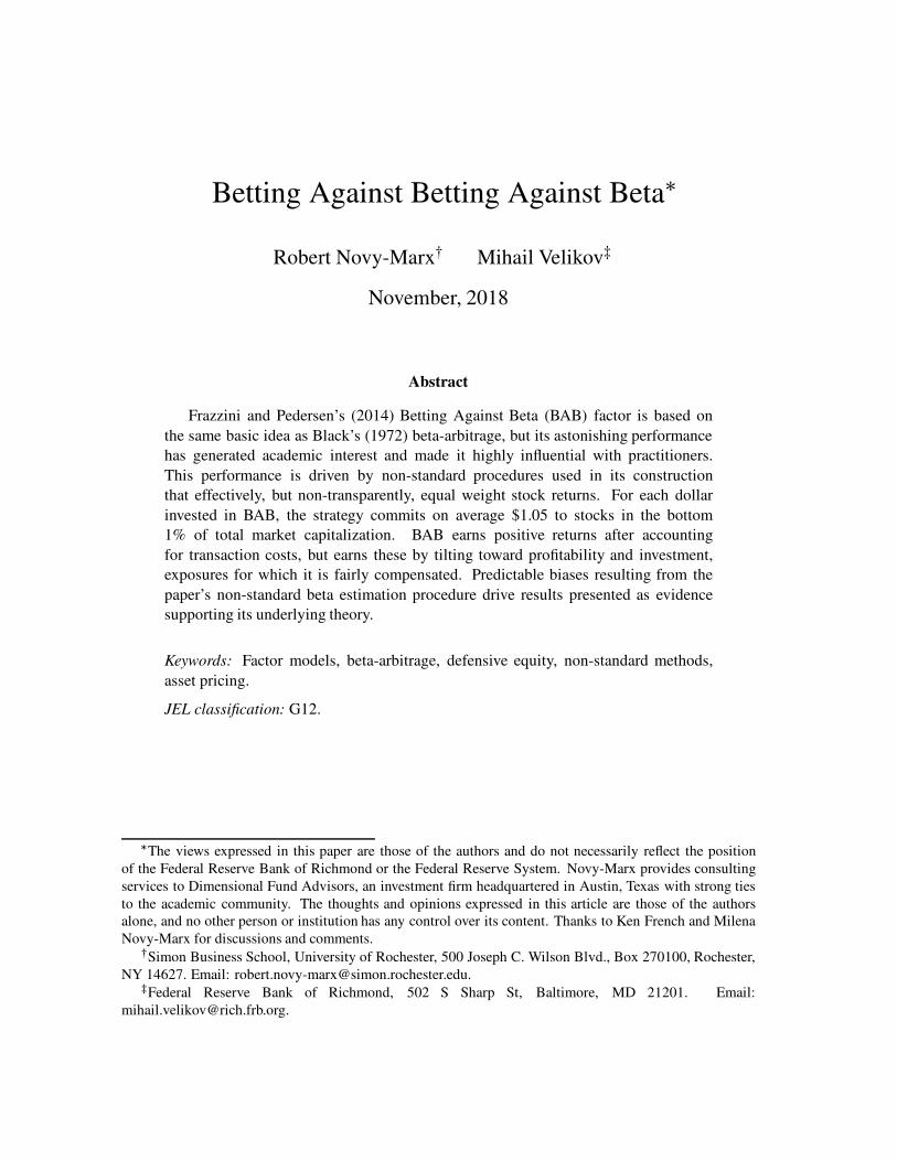
Betting Against Betting Against Beta�

Robert Novy-Marx� Mihail Velikov�

November, 2018

Abstract

Frazzini and Pedersen’s (2014) Betting Against Beta (BAB) factor is based on

the same basic idea as Black’s (1972) beta-arbitrage, but its astonishing performance

has generated academic interest and made it highly influential with practitioners.

This performance is driven by non-standard procedures used in its construction

that effectively, but non-transparently, equal weight stock returns. For each dollar

invested in BAB, the strategy commits on average $1.05 to stocks in the bottom

1% of total market capitalization. BAB earns positive returns after accounting

for transaction costs, but earns these by tilting toward profitability and investment,

exposures for which it is fairly compensated. Predictable biases resulting from the

paper’s non-standard beta estimation procedure drive results presented as evidence

supporting its underlying theory.

Keywords: Factor models, beta-arbitrage, defensive equity, non-standard methods,

asset pricing.

JEL classification: G12.

�The views expressed in this paper are those of the authors and do not necessarily reflect the position

of the Federal Reserve Bank of Richmond or the Federal Reserve System. Novy-Marx provides consulting

services to Dimensional Fund Advisors, an investment firm headquartered in Austin, Texas with strong ties

to the academic community. The thoughts and opinions expressed in this article are those of the authorsalone, and no other person or institution has any control over its content. Thanks to Ken French and Milena

Novy-Marx for discussions and comments.�Simon Business School, University of Rochester, 500 Joseph C. Wilson Blvd., Box 270100, Rochester,

NY 14627. Email: robert.novy-marx@simon.rochester.edu.�Federal Reserve Bank of Richmond, 502 S Sharp St, Baltimore, MD 21201. Email:

mihail.velikov@rich.frb.org.

1. Introduction

Frazzini and Pedersen’s (FP) Betting Against Beta (BAB, 2014) is an unmitigated

academic success. It is, at the time of this writing, the fourth most downloaded article from

the Journal of Financial Economics over the last 90 days, and its field-weighted citation

impact suggests it has been cited 26 times more often than the average paper published

in similar journals. Its impact on practice has been even greater. It is one of the most

influential articles on “defensive equity,” a class of strategies that has seen massive capital

inflows and is now a major investment category for institutional investors.

This success is particularly remarkable because BAB is based on a fairly simple idea

that predates its publication by more than 40 years. Black (1972) first suggested trading to

exploit an empirical failure of the Capital Asset Pricing Model (CAPM): the fact that the

observed Capital Market Line is “too flat.” Low beta stocks have earned higher average

returns than predicted by the CAPM, while high beta stocks have underperformed the

model’s predictions, so strategies that overweight low beta stocks and underweight high

beta stocks have earned positive CAPM alphas.

Despite being widely read, and based on a fairly simple idea, BAB is not well

understood. This is because the authors use three unconventional procedures to construct

their factor. All three departures from standard factor construction contribute to the paper’s

strong empirical results. None is important for understanding the underlying economics,

and each obscures the mechanisms driving reported effects.

Two of these non-standard procedures drive BAB’s astonishing “paper” performance,

which cannot be achieved in practice, while the other drives results FP present as evidence

supporting their theory. The two responsible for driving performance can be summarized

as follows:

1

Non-standard procedure #1, rank-weighted portfolio construction: Instead of

simply sorting stocks when constructing the beta portfolios underlying BAB, FP use

a “rank-weighting” procedure that assigns each stock to either the “high” portfolio

or the “low” portfolio with a weight proportional to the cross-sectional deviation of

the stock’s estimated beta rank from the median rank.

Non-standard procedure #2, hedging by leveraging: Instead of hedging the low

beta-minus-high beta strategy underlying BAB by buying the market in proportion

to the underlying strategy’s observed short market tilt, FP attempt to achieve

market-neutrality by leveraging the low beta portfolio and deleveraging the high beta

portfolio using these portfolios’ predicted betas, with the intention that the scaled

portfolios’ betas are each equal to one and thus net to zero in the long/short strategy.

FP’s first of these non-standard procedures, rank-weighting, drives BAB’s performance

not by what it does, i.e., put more weight on stocks with extreme betas, but by what it does

not do, i.e., weight stocks in proportion to their market capitalizations, as is standard in asset

pricing. The procedure creates portfolios that are almost indistinguishable from simple,

equal-weighted portfolios. Their second non-standard procedure, hedging with leverage,

uses these same portfolios to hedge the low beta-minus-high beta strategy underlying BAB.

That is, the rank-weighting procedure is a backdoor to equal-weighting the underlying beta

portfolios, and the leveraging procedure is a backdoor to using equal-weighted portfolios

for hedging.

BAB achieves its high Sharpe ratio, and large, highly significant alpha relative to the

common factor models, by hugely overweighting micro- and nano-cap stocks. For each

dollar invested in BAB, the strategy commits on average $1.05 to stocks in the bottom

1% of total market capitalization. These stocks have limited capacity and are expensive to

trade. As a result, while BAB’s “paper” performance is impressive, it is not something an

2

investor can actually realize. Accounting for transaction costs reduces BAB’s profitability

by almost 60%. While it still earns significant positive returns, it earns these by tilting

toward profitability and investment, exposures for which it is fairly compensated. It does

not have a significant net alpha relative to the Fama and French (2015) five-factor model.

The third non-standard procedure FP use when constructing BAB, a novel method

for estimating betas, mechanically generates results they present as empirical evidence

supporting their paper’s underlying theory. One of the paper’s main theoretical predictions

is “beta compression,” specifically that the market “betas of securities in the cross section

are compressed toward one when funding liquidity risk is high” (p. 2). To support this

prediction, they present evidence that the cross-sectional dispersion in betas is negatively

correlated with TED-spread volatility, which they use as a proxy for funding liquidity

risk. This result actually reflects biases resulting from their non-standard beta estimation

procedure.

FP’s non-standard beta estimation procedure works as follows:

Non-standard procedure #3, novel beta estimation technique: Instead of

estimating betas as slope coefficients from CAPM regressions, FP measure betas by

combining market correlations estimated using five years of overlapping three-day

returns with volatilities estimated using one year of daily data.

FP justify this procedure by stating that they estimate betas using “one-year rolling standard

deviation for volatilities and a five-year horizon for the correlation to account for the

fact that correlations appear to move more slowly than volatilities” (p. 8). While this

justification may sound appealing, and the method has seen significant adoption in the

literature that follows BAB, the procedure does not actually yield market betas. This is

3

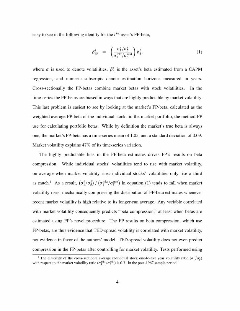
easy to see in the following identity for the i th asset’s FP-beta,

ˇiFP D

�� i

1=� i5

�mkt1 =�mkt

5

�

ˇi5; (1)

where � is used to denote volatilities, ˇi5 is the asset’s beta estimated from a CAPM

regression, and numeric subscripts denote estimation horizons measured in years.

Cross-sectionally the FP-betas combine market betas with stock volatilities. In the

time-series the FP-betas are biased in ways that are highly predictable by market volatility.

This last problem is easiest to see by looking at the market’s FP-beta, calculated as the

weighted average FP-beta of the individual stocks in the market portfolio, the method FP

use for calculating portfolio betas. While by definition the market’s true beta is always

one, the market’s FP-beta has a time-series mean of 1.05, and a standard deviation of 0.09.

Market volatility explains 47% of its time-series variation.

The highly predictable bias in the FP-beta estimates drives FP’s results on beta

compression. While individual stocks’ volatilities tend to rise with market volatility,

on average when market volatility rises individual stocks’ volatilities only rise a third

as much.1 As a result,�

� i1=� i

5

�

=�

�mkt1 =�mkt

5

�

in equation (1) tends to fall when market

volatility rises, mechanically compressing the distribution of FP-beta estimates whenever

recent market volatility is high relative to its longer-run average. Any variable correlated

with market volatility consequently predicts “beta compression,” at least when betas are

estimated using FP’s novel procedure. The FP results on beta compression, which use

FP-betas, are thus evidence that TED-spread volatility is correlated with market volatility,

not evidence in favor of the authors’ model. TED-spread volatility does not even predict

compression in the FP-betas after controlling for market volatility. Tests performed using

1 The elasticity of the cross-sectional average individual stock one-to-five year volatility ratio (� i1=� i

5)

with respect to the market volatility ratio (�mkt1 =�mkt

5 ) is 0.31 in the post-1967 sample period.

4

market betas instead of the biased FP-betas provide no support for the paper’s theory.

The biased FP-betas are also used in FP’s hedging procedure, with the result that BAB is

not market-neutral, contrary to FP’s intent. Market volatility predicts the FP-beta estimates

of the underlying beta portfolios, which are used to hedge these portfolios, but not the

actual betas of these underlying portfolios. Market volatility consequently also predicts

the severity of BAB’s mis-hedging, and thus its conditional beta. This fact makes the

results that FP present on BAB’s conditional market tilts difficult to interpret. They offer

the results as support for the paper’s underlying theory, but because of their non-standard

construction methods any variable correlated with market volatility mechanically predicts

BAB’s mis-hedging, and thus its conditional beta.

These facts raise a question: how can a paper be so influential, and so well read, yet

so poorly understood? Our paper provides an answer, by highlighting the role that each

of BAB’s non-standard, non-transparent procedures plays in generating its strong results.

While our paper’s specific focus is BAB, its intended message is general: results dependent

on non-standard methods should be evaluated cautiously.

2. Alternative procedures driving BAB’s performance

This section quantifies the impact FP’s non-standard portfolio construction procedure

and non-standard hedging procedure have on BAB’s performance.2 It does so by comparing

the performance of BAB to similarly constructed “almost BAB” strategies, which differ

from BAB only by using standard methods for either portfolio construction or hedging.

These comparisons obviously require the performance of BAB, the yardstick against

which we measure the “almost BAB” variations. This involves a choice, as there is

2 Li, Novy-Marx, and Velikov (2018) also look at the impact of non-standard methods, analyzing their

impact on the performance of liquidity strategies.

5

not a single “canonical” BAB strategy. BAB’s returns are maintained by AQR Capital

Management. While FP present some results for other asset classes, AQR only updates the

equity factors, and we similarly limit our focus. AQR makes available the “original paper

dataset,” which ends after March 2012, and a “BAB equity factor,” which is “an updated and

extended version of the paper data.”3 Unfortunately these two factors differ. The monthly

correlation between the two US equity factors is 96.2% in the post-1967 sample, but the

original series has a significantly higher Sharpe ratio than the currently maintained series.4

When we replicate BAB using the construction methods described by FP, our factor has a

monthly correlation of 98.5% with FP’s original series, and realizes the same 1.01 Sharpe

ratio over the January 1968 to March 2012 sample period.5 Overall, our BAB replication is

quite similar to the original paper series, and is directly comparable to the “almost BAB”

strategies we consider next, because it is constructed using exactly the same data. It is

also available beyond the original series’ March 2012 end date. We consequently use our

replication of BAB as the yardstick against which we evaluate the strategies.

2.1. Rank-weighting versus standard portfolio sorts

When FP construct the beta portfolios underlying BAB, the weight on each stock is

proportional to the difference between the stock’s cross-sectional characteristic rank, ri ,

3 These data can be found at https://www.aqr.com/Insights/Datasets/.4 We follow Baker, Bradley, and Wurgler (2011) in starting our sample at the beginning of 1968, a

common start date for the literature on “defensive” strategies. Extending the sample beyond 50 years does

not change any qualitative conclusions, but does preclude the use of the Fama and French (2015) profitability

and investment factors in the asset pricing tests, as these are only available after June 1963.5 A detailed comparison of the three different versions of BAB is provided in Appendix A.

6

and the median rank, rmedian,

wi D

8

ˆˆ

<

ˆˆ

:

.ri � rmedian/P

fj jrj <rmediang

�

rj � rmedian

� if ri < rmedian (low beta portfolio),

.ri � rmedian/P

fj jrj >rmediang

�

rj � rmedian

� if ri > rmedian (high beta portfolio).

Note that firm size is not considered when constructing rank-weighted portfolios.6

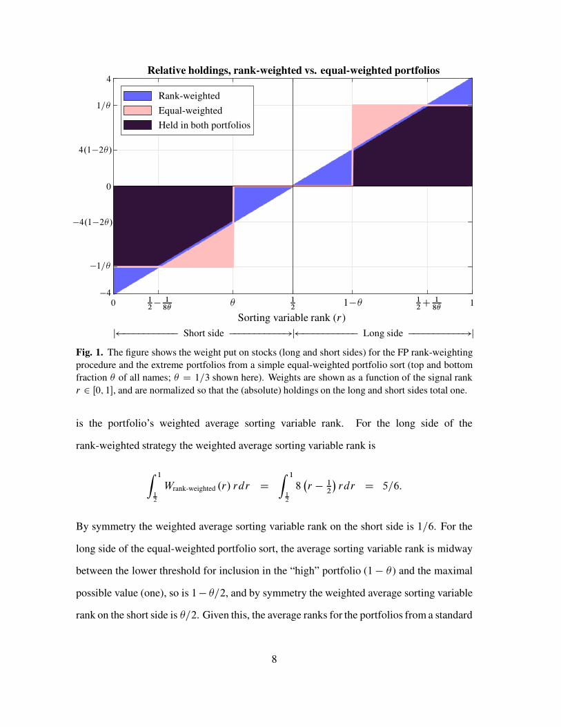
Figure 1 shows the relative weights on stocks in the long/short strategy under the FP

rank-weighting procedure, and in a standard equal-weighted portfolio that holds the top

fraction � of all stocks, while shorting the bottom � (in the figure � is 1/3). The horizontal

axis is the cross-sectional rank of the sorting variable, r , from zero to one. Normalizing so

that the total weight in each portfolio is one, the weights on the stock with rank r in the two

portfolios shown in the figure are:

Wrank-weighted .r/ D 8�

r � 12

�

Wequal-weighted .r/ D

8

ˆˆ

<

ˆˆ

:

1�

if r > 1 � �

� 1�

if r < �

0 otherwise.

A useful heuristic that measures how hard a portfolio “tilts” toward a given strategy

6 There is no reason that a rank-weighting procedure has to ignore market capitalizations. A rank- and

capitalization-weighted scheme retains the spirit of rank-weighting, by over-weighting extreme observations,

while simultaneously creating portfolios that are largely representative of the size distribution observed in the

market. Under this procedure the weight on stock i with signal rank ri is equal to

wi D

8

ˆˆ<

ˆˆˆ:

.ri � rmedian/ MarketCapiP

fj jrj <rmediang

�

rj � rmedian

�

MarketCapj

if ri < rmedian,

.ri � rmedian/ MarketCapiP

fj jrj >rmediang

�

rj � rmedian

�

MarketCapj

if ri > rmedian.

7

Relative holdings, rank-weighted vs. equal-weighted portfolios

Rank-weighted

Equal-weighted

Held in both portfolios

4

1=�

4.1�2�/

0

�4.1�2�/

�1=�

�40 1

2� 1

8�� 1

21�� 1

2C 1

8�1

Sorting variable rank (r)

j ����������� Short side �����������!j ����������� Long side �����������!j

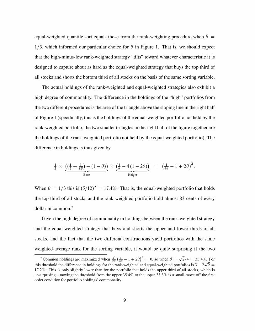
Fig. 1. The figure shows the weight put on stocks (long and short sides) for the FP rank-weighting

procedure and the extreme portfolios from a simple equal-weighted portfolio sort (top and bottom

fraction � of all names; � D 1=3 shown here). Weights are shown as a function of the signal rank

r 2 Œ0; 1�, and are normalized so that the (absolute) holdings on the long and short sides total one.

is the portfolio’s weighted average sorting variable rank. For the long side of the

rank-weighted strategy the weighted average sorting variable rank is

Z 1

12

Wrank-weighted .r/ rdr DZ 1

12

8�

r � 12

�

rdr D 5=6:

By symmetry the weighted average sorting variable rank on the short side is 1=6. For the

long side of the equal-weighted portfolio sort, the average sorting variable rank is midway

between the lower threshold for inclusion in the “high” portfolio (1 � � ) and the maximal

possible value (one), so is 1� �=2, and by symmetry the weighted average sorting variable

rank on the short side is �=2. Given this, the average ranks for the portfolios from a standard

8

equal-weighted quantile sort equals those from the rank-weighting procedure when � D

1=3, which informed our particular choice for � in Figure 1. That is, we should expect

that the high-minus-low rank-weighted strategy “tilts” toward whatever characteristic it is

designed to capture about as hard as the equal-weighted strategy that buys the top third of

all stocks and shorts the bottom third of all stocks on the basis of the same sorting variable.

The actual holdings of the rank-weighted and equal-weighted strategies also exhibit a

high degree of commonality. The difference in the holdings of the “high” portfolios from

the two different procedures is the area of the triangle above the sloping line in the right half

of Figure 1 (specifically, this is the holdings of the equal-weighted portfolio not held by the

rank-weighted portfolio; the two smaller triangles in the right half of the figure together are

the holdings of the rank-weighted portfolio not held by the equal-weighted portfolio). The

difference in holdings is thus given by

12���

12C 1

8�

�

� .1 � �/�

„ ƒ‚ …

Base

��

1�� 4 .1 � 2�/

�

„ ƒ‚ …

Height

D�

14�� 1C 2�

�2:

When � D 1=3 this is .5=12/2 D 17:4%. That is, the equal-weighted portfolio that holds

the top third of all stocks and the rank-weighted portfolio hold almost 83 cents of every

dollar in common.7

Given the high degree of commonality in holdings between the rank-weighted strategy

and the equal-weighted strategy that buys and shorts the upper and lower thirds of all

stocks, and the fact that the two different constructions yield portfolios with the same

weighted-average rank for the sorting variable, it would be quite surprising if the two

7 Common holdings are maximized when dd�

�1

4�� 1C 2�

�2 D 0, so when � Dp

2=4 D 35:4%. For

this threshold the difference in holdings for the rank-weighted and equal-weighted portfolios is 3 � 2p

2 D17:2%. This is only slightly lower than for the portfolio that holds the upper third of all stocks, which is

unsurprising—moving the threshold from the upper 35.4% to the upper 33.3% is a small move off the first

order condition for portfolio holdings’ commonality.

9

1968 1973 1978 1983 1988 1993 1998 2003 2008 2013 2018

$1

$10

$100

BAB vs. portfolio sorted BAB

BAB

Equal-weighted BAB

Value-weighted BAB

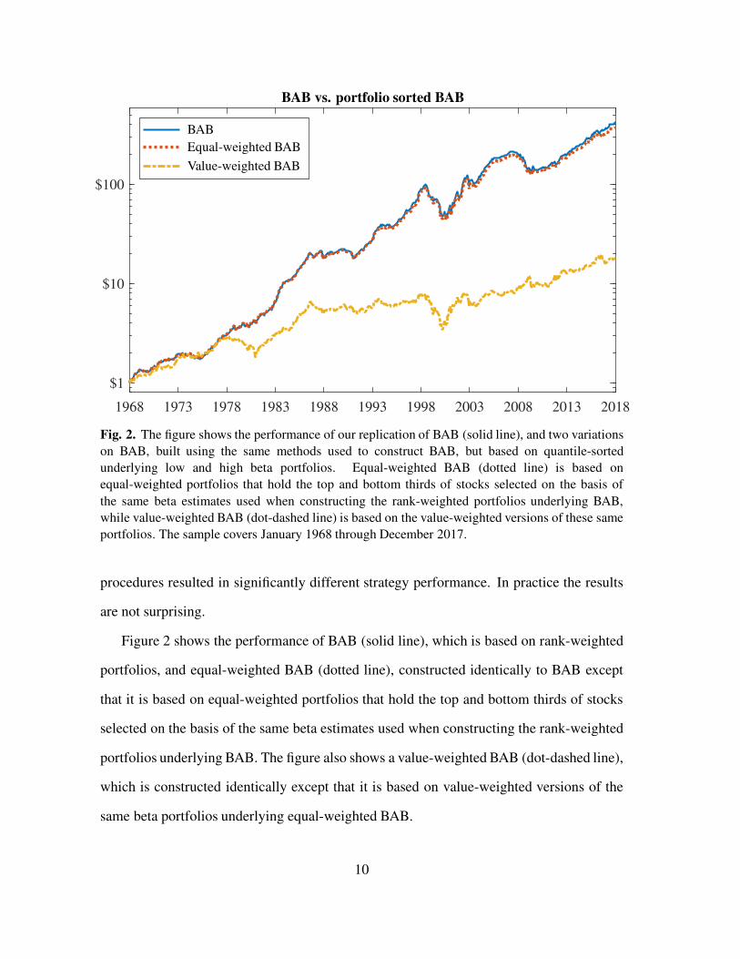
Fig. 2. The figure shows the performance of our replication of BAB (solid line), and two variations

on BAB, built using the same methods used to construct BAB, but based on quantile-sorted

underlying low and high beta portfolios. Equal-weighted BAB (dotted line) is based on

equal-weighted portfolios that hold the top and bottom thirds of stocks selected on the basis of

the same beta estimates used when constructing the rank-weighted portfolios underlying BAB,

while value-weighted BAB (dot-dashed line) is based on the value-weighted versions of these same

portfolios. The sample covers January 1968 through December 2017.

procedures resulted in significantly different strategy performance. In practice the results

are not surprising.

Figure 2 shows the performance of BAB (solid line), which is based on rank-weighted

portfolios, and equal-weighted BAB (dotted line), constructed identically to BAB except

that it is based on equal-weighted portfolios that hold the top and bottom thirds of stocks

selected on the basis of the same beta estimates used when constructing the rank-weighted

portfolios underlying BAB. The figure also shows a value-weighted BAB (dot-dashed line),

which is constructed identically except that it is based on value-weighted versions of the

same beta portfolios underlying equal-weighted BAB.

10

The figure shows that BAB and equal-weighted BAB have almost identical

performance. In fact, the two strategies are 99.6% correlated at the monthly frequency, and

earn statistically indistinguishable average returns. That is, the rank-weighting procedure

of FP, while more complicated and more difficult to implement, is essentially identical to a

simple equal-weighted portfolio sort. This close correspondence is not limited to strategies

based on beta portfolios. Appendix B shows that rank-weighted value and momentum are

also basically identical to their equal-weighted portfolio-sorted counterparts.

While the rank-weighting procedure yields portfolio performance that is essentially

indistinguishable from simple equal-weighted quantile sorting, it is nevertheless the single

largest driver of BAB’s astonishing performance. This can be seen by contrasting

the performance of BAB (or equal-weighted BAB) with that of value-weighted BAB.

Value-weighted performance is generally more interesting, because it more accurately

reflects what investors can achieve in practice. The performance of the value-weighed

version of BAB is much less impressive. Value-weighted BAB earns significant positive

excess returns over the sample, 56 bps/month with a t-statistic of 3.48, but its Sharpe ratio

is less than half as large as BAB’s (0.49 compared to 1.08).8 It also earns most of these

returns by tilting strongly to profitability and investment (loadings of 0.45 on RMW and

0.50 on CMA, with t-statistics of 6.59 and 4.86, respectively). The strategy’s alpha relative

to the Fama and French five-factor model is only 24 bps/month, and insignificant (t-statistic

of 1.63).9

8 This is similar to the 51 bps/month return spread FP report for “value-weighted BAB” in Table B9

of their online appendix. The high and low beta portfolios underlying FP’s value-weighted BAB are eachconstructed as equal-weighted averages of small and large capitalization strategies, along the lines of how

Fama and French (1993) build HML. Specifically, the high beta portfolio is a 50/50 combination of the

value-weighted portfolios that hold only high beta stocks (top 30%) with either above or below median NYSE

market capitalizations, and the low beta portfolio is constructed similarly. FP’s “value-weighted BAB” by

construction consequently puts half its weight on small stocks that make up on average less than 11% of total

market capitalization, and thus cannot accurately be described as “value-weighted.”9 Its alpha relative to the six-factor model that also includes momentum is even lower, 14 bps/month with

a t-statistic of 0.93. A detailed analysis of the performance of this strategy, and all the strategies considered

here, is provided in Appendix C.

11

2.2. Hedging by leveraging versus simple direct hedging

In their second major deviation from standard factor construction techniques, FP

attempt to make BAB market-neutral using leverage. They scale the underlying portfolios

by their predicted betas, with the intention that the leveraged, low beta portfolio and the

deleveraged, high beta portfolio each individually have betas of one, and thus net to zero in

the long/short strategy.10

The simple, standard alternative is to buy the market in proportion to the underlying low

beta-minus-high beta strategy’s short market tilt, financing the long market position through

borrowing. While conceptually it makes sense to hedge using the value-weighted market

portfolio, the strategy that results from doing so, “directly hedged BAB,” is quite dissimilar

to BAB. This is because BAB is constructed by hedging an underlying dollar-neutral low

beta-minus-high beta strategy by buying rank-weighted portfolios, a fact apparent in the

10 This procedure is biased, because of Jensen’s inequality and the fact that betas are estimated with noise.

If zero is in the continuous support of a portfolio’s potential beta estimate, then expected leverage (inverseof the estimated beta) is unbounded, and so is the leveraged portfolio’s true expected beta. More generally,

suppose that a portfolio’s true beta is measured with noise, O D ˇ.1C �/ where � is mean-zero proportional

estimation error. Then the expected beta of the portfolio held in inverse proportion to its estimated beta is

E

"

ˇ

O

#

D E

�1

1C �

�

D 1C1X

iD2

Eh

.��/ii

:

That is, the expected beta of a portfolio scaled by the inverse of its estimated beta differs from one by the

difference between the sums of the even and the higher odd central moments of the noise with which beta

is estimated. Under the reasonable assumption that the estimation error is symmetric (or nearly symmetric),

the odd moments are zero (or close to zero), and the expected bias is simply (roughly) the sum of the evencentral moments. In this case, scaling a portfolio by the portfolio’s estimated beta yields a strategy that has

an expected beta greater than one.

12

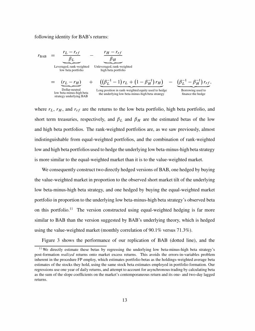
following identity for BAB’s returns:

rBAB DrL � rrf

ˇL„ ƒ‚ …

Leveraged, rank-weightedlow beta portfolio

� rH � rrf

ˇH„ ƒ‚ …

Unleveraged, rank-weightedhigh beta portfolio

D .rL � rH /„ ƒ‚ …

Dollar-neutrallow beta-minus-high betastrategy underlying BAB

C��

ˇ�1L � 1

�

rL C�

1 � ˇ�1H

�

rH

�

„ ƒ‚ …

Long position in rank-weighted equity used to hedgethe underlying low beta-minus-high beta strategy

��

ˇ�1L � ˇ�1

H

�

rrf„ ƒ‚ …

Borrowing used tofinance the hedge

;

where rL, rH , and rrf are the returns to the low beta portfolio, high beta portfolio, and

short term treasuries, respectively, and ˇL and ˇH are the estimated betas of the low

and high beta portfolios. The rank-weighted portfolios are, as we saw previously, almost

indistinguishable from equal-weighted portfolios, and the combination of rank-weighted

low and high beta portfolios used to hedge the underlying low beta-minus-high beta strategy

is more similar to the equal-weighted market than it is to the value-weighted market.

We consequently construct two directly hedged versions of BAB, one hedged by buying

the value-weighted market in proportion to the observed short market tilt of the underlying

low beta-minus-high beta strategy, and one hedged by buying the equal-weighted market

portfolio in proportion to the underlying low beta-minus-high beta strategy’s observed beta

on this portfolio.11 The version constructed using equal-weighted hedging is far more

similar to BAB than the version suggested by BAB’s underlying theory, which is hedged

using the value-weighted market (monthly correlation of 90.1% versus 71.3%).

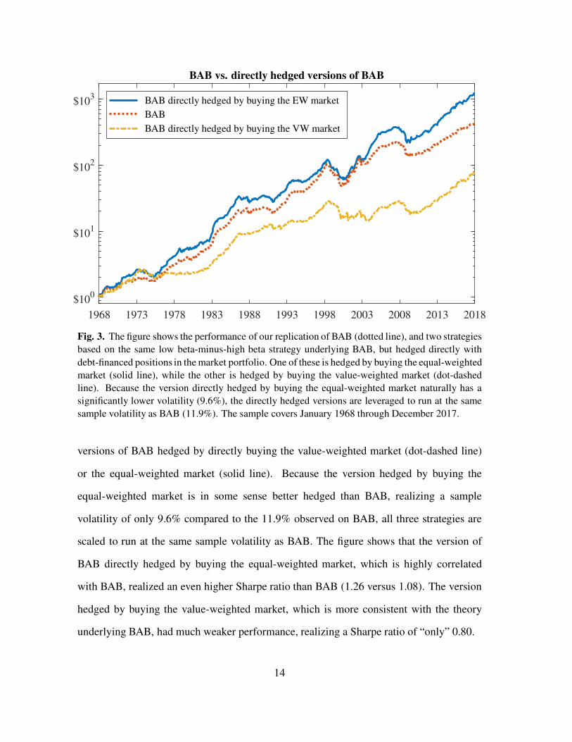
Figure 3 shows the performance of our replication of BAB (dotted line), and the

11 We directly estimate these betas by regressing the underlying low beta-minus-high beta strategy’s

post-formation realized returns onto market excess returns. This avoids the errors-in-variables problem

inherent in the procedure FP employ, which estimates portfolio betas as the holdings-weighted average beta

estimates of the stocks they hold, using the same stock beta estimates employed in portfolio formation. Our

regressions use one year of daily returns, and attempt to account for asynchronous trading by calculating betaas the sum of the slope coefficients on the market’s contemporaneous return and its one- and two-day lagged

returns.

13

1968 1973 1978 1983 1988 1993 1998 2003 2008 2013 2018

$100

$101

$102

$103

BAB vs. directly hedged versions of BAB

BAB directly hedged by buying the EW market

BAB

BAB directly hedged by buying the VW market

Fig. 3. The figure shows the performance of our replication of BAB (dotted line), and two strategies

based on the same low beta-minus-high beta strategy underlying BAB, but hedged directly with

debt-financed positions in the market portfolio. One of these is hedged by buying the equal-weighted

market (solid line), while the other is hedged by buying the value-weighted market (dot-dashed

line). Because the version directly hedged by buying the equal-weighted market naturally has a

significantly lower volatility (9.6%), the directly hedged versions are leveraged to run at the same

sample volatility as BAB (11.9%). The sample covers January 1968 through December 2017.

versions of BAB hedged by directly buying the value-weighted market (dot-dashed line)

or the equal-weighted market (solid line). Because the version hedged by buying the

equal-weighted market is in some sense better hedged than BAB, realizing a sample

volatility of only 9.6% compared to the 11.9% observed on BAB, all three strategies are

scaled to run at the same sample volatility as BAB. The figure shows that the version of

BAB directly hedged by buying the equal-weighted market, which is highly correlated

with BAB, realized an even higher Sharpe ratio than BAB (1.26 versus 1.08). The version

hedged by buying the value-weighted market, which is more consistent with the theory

underlying BAB, had much weaker performance, realizing a Sharpe ratio of “only” 0.80.

14

While FP’s leveraging procedure does not yield stronger performance than directly

beta-hedging the underlying low beta-minus-high beta strategy with the equal-weighted

market, it is nevertheless crucial, like rank-weighting, for delivering BAB’s astonishing

performance. Hedging with equal-weighted portfolios instead of value-weighted portfolios

contributes significantly to performance, and while not explicit in FP, the leveraging

procedure is the backdoor through which the paper implements equal-weighted hedging.

The leveraging procedure uses the underlying portfolios to do the hedging, and in BAB’s

case these are rank-weighted, and thus almost indistinguishable from equal-weighted

portfolios. Using these portfolios instead of the market to hedge the underlying strategy’s

short market tilt contributes significantly to BAB’s strong paper performance.

3. Implementing BAB

FP’s rank-weighting procedure creates underlying beta portfolios that are almost

indistinguishable from equal-weighted portfolios, and FP’s leveraging procedure uses these

same portfolios to hedge the strategy. As a result, the strategy dramatically over-weights

the smallest, most illiquid stocks, making it infeasible in practice.

To understand how acute BAB’s equal-weighting problem is, we can look at the actual

weights the strategy puts on stocks from different size “universes.” Table 1 does this,

where the size universes are size deciles formed using NYSE breaks. These divide the

market into ten buckets based on market capitalization, where the breaks are set so that,

by construction, 10% of NYSE stocks fall into each. NASDAQ and AMEX stocks tend to

be smaller, so are more likely to fall into the smaller stock portfolios. To provide a sense

of the kinds of stocks held in each universe, the second column of the table shows the

smallest stock held in each at the end of the sample. For example, at the end of the sample

“large stocks,” under the Fama and French (2008) definition of those with above NYSE

15

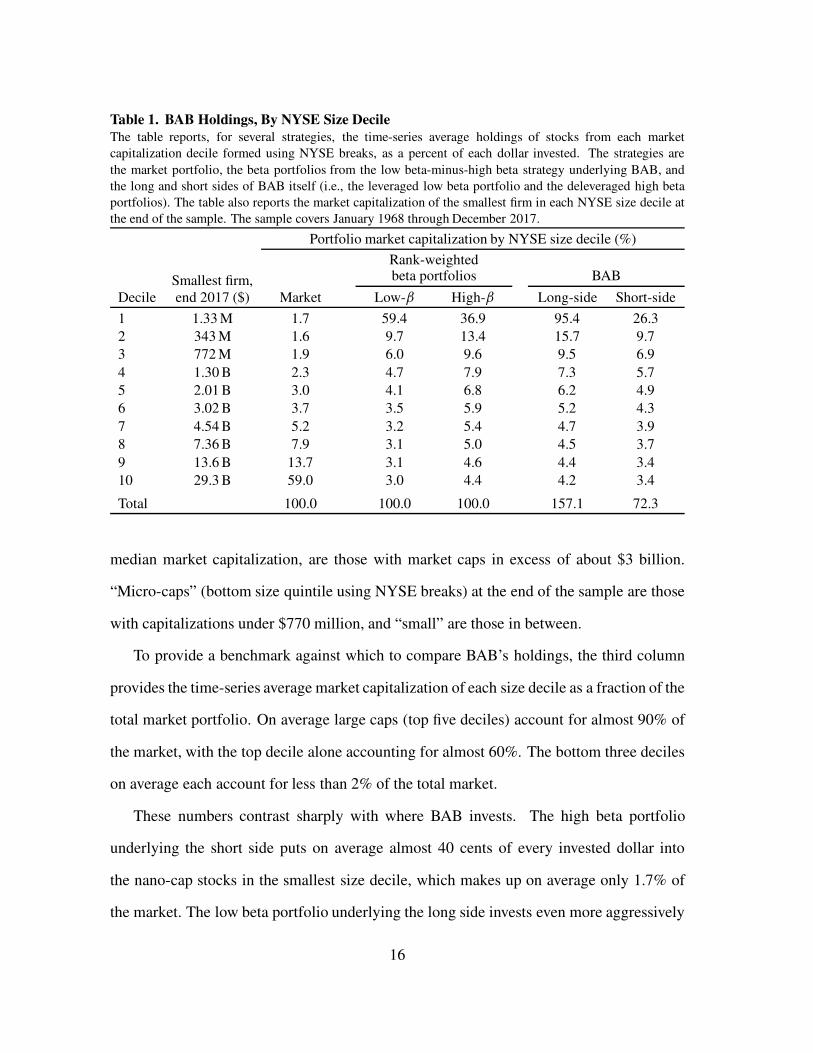
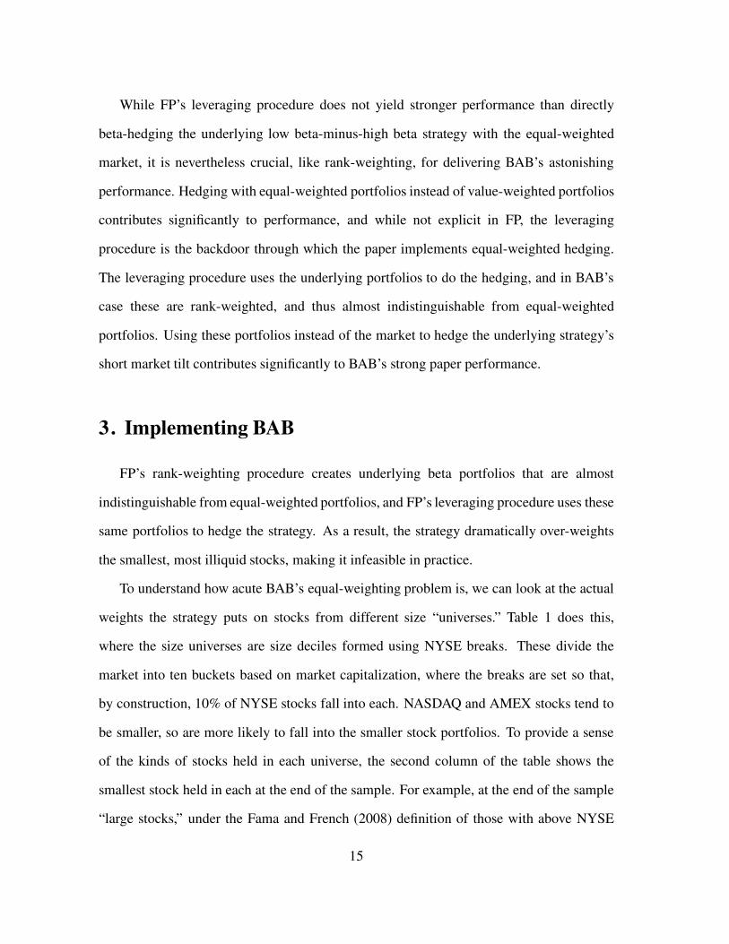
Table 1. BAB Holdings, By NYSE Size Decile

The table reports, for several strategies, the time-series average holdings of stocks from each market

capitalization decile formed using NYSE breaks, as a percent of each dollar invested. The strategies are

the market portfolio, the beta portfolios from the low beta-minus-high beta strategy underlying BAB, and

the long and short sides of BAB itself (i.e., the leveraged low beta portfolio and the deleveraged high beta

portfolios). The table also reports the market capitalization of the smallest firm in each NYSE size decile at

the end of the sample. The sample covers January 1968 through December 2017.

Portfolio market capitalization by NYSE size decile (%)

Rank-weightedbeta portfolios BABSmallest firm,

Decile end 2017 ($) Market Low-ˇ High-ˇ Long-side Short-side

1 1.33 M 1.7 59.4 36.9 95.4 26.3

2 343 M 1.6 9.7 13.4 15.7 9.7

3 772 M 1.9 6.0 9.6 9.5 6.9

4 1.30 B 2.3 4.7 7.9 7.3 5.7

5 2.01 B 3.0 4.1 6.8 6.2 4.9

6 3.02 B 3.7 3.5 5.9 5.2 4.3

7 4.54 B 5.2 3.2 5.4 4.7 3.9

8 7.36 B 7.9 3.1 5.0 4.5 3.7

9 13.6 B 13.7 3.1 4.6 4.4 3.4

10 29.3 B 59.0 3.0 4.4 4.2 3.4

Total 100.0 100.0 100.0 157.1 72.3

median market capitalization, are those with market caps in excess of about $3 billion.

“Micro-caps” (bottom size quintile using NYSE breaks) at the end of the sample are those

with capitalizations under $770 million, and “small” are those in between.

To provide a benchmark against which to compare BAB’s holdings, the third column

provides the time-series average market capitalization of each size decile as a fraction of the

total market portfolio. On average large caps (top five deciles) account for almost 90% of

the market, with the top decile alone accounting for almost 60%. The bottom three deciles

on average each account for less than 2% of the total market.

These numbers contrast sharply with where BAB invests. The high beta portfolio

underlying the short side puts on average almost 40 cents of every invested dollar into

the nano-cap stocks in the smallest size decile, which makes up on average only 1.7% of

the market. The low beta portfolio underlying the long side invests even more aggressively

16

in these nano-caps, putting on average almost 60 cents of every invested dollar into these

stocks. BAB itself, because it leverages this low beta portfolio on average by more than

50%, puts an average of 95.4 cents of every dollar into low beta stocks in the smallest

decile, while shorting 26.3 of high beta stocks there. On net, for every dollar invested in

BAB, the strategy takes equity positions that on average exceed $1.20 in these stocks that

make up the bottom 1.7% of the market.12 This presents significant implementation issues,

because the smallest stocks have limited capacity and are expensive to trade.

3.1. The cost of trading BAB

BAB dramatically overweights nano- and micro-cap stocks that are expensive to trade,

making it far less profitable in practice than on paper. We can get a sense of how difficult

BAB is to trade by calculating the strategy’s average turnover in each NYSE size decile.

Table 2 gives this turnover, as a fraction of the total capital invested in the strategy. Overall,

BAB entails significant trading, and like its holdings, this trading is heavily concentrated in

the smallest stocks. Each dollar invested in the strategy is associated on average with more

than two dollars of annual turnover (214.7% per year), with $1.33 of round trip trading

on the long side and $0.82 of round trip trading on the short side. While this turnover is

not especially high (roughly three times the turnover of a value strategy, but only a third

the turnover of momentum), almost two thirds of this trading is in nano-cap stocks in the

smallest NYSE size decile (121.1% per year), and these stocks are expensive to trade.

This turnover translates into significant transaction costs, averaging 60 bps/month,

calculated using the methodology of Novy-Marx and Velikov (2016).13 These costs

dramatically reduce the performance a BAB investor would have realized in practice.

12 If we define nano-cap more narrowly, as the bottom 1% of market capitalization, BAB’s equity position

in nano-caps averages “only” $1.05. Almost a third of this is in stocks that make up the bottom 0.1% of the

market, firms with end of sample market capitalizations under $92 million.13 These costs averaged only 26 bps/month over the last ten years of the sample. Despite this BAB was

less profitable to trade over this period, because it also realized significantly lower gross returns.

17

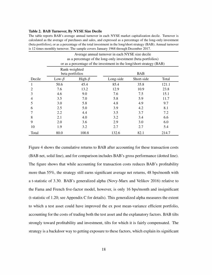
Table 2. BAB Turnover, By NYSE Size Decile

The table reports BAB’s average annual turnover in each NYSE market capitalization decile. Turnover is

calculated as the average of purchases and sales, and expressed as a percentage of the long-only investment

(beta portfolios), or as a percentage of the total investment in the long/short strategy (BAB). Annual turnover

is 12 times monthly turnover. The sample covers January 1968 through December 2017.

Average annual turnover in each NYSE size decile

as a percentage of the long-only investment (beta portfolios)

or as a percentage of the investment in the long/short strategy (BAB)

Rank-weightedbeta portfolios BAB

Decile Low-ˇ High-ˇ Long-side Short-side Total

1 50.6 45.4 85.4 35.8 121.1

2 7.6 13.2 12.9 10.9 23.8

3 4.6 9.0 7.6 7.5 15.1

4 3.5 7.0 5.8 5.9 11.7

5 3.0 5.8 4.8 4.9 9.7

6 2.5 5.0 3.9 4.2 8.1

7 2.2 4.4 3.5 3.7 7.2

8 2.1 4.0 3.2 3.4 6.6

9 2.0 3.6 2.9 3.0 6.0

10 1.9 3.2 2.7 2.7 5.4

Total 80.0 100.8 132.6 82.1 214.7

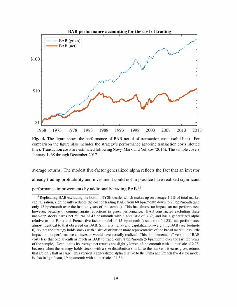
Figure 4 shows the cumulative returns to BAB after accounting for these transaction costs

(BAB net, solid line), and for comparison includes BAB’s gross performance (dotted line).

The figure shows that while accounting for transaction costs reduces BAB’s profitability

more than 55%, the strategy still earns significant average net returns, 48 bps/month with

a t-statistic of 3.30. BAB’s generalized alpha (Novy-Marx and Velikov 2016) relative to

the Fama and French five-factor model, however, is only 16 bps/month and insignificant

(t-statistic of 1.20; see Appendix C for details). This generalized alpha measures the extent

to which a test asset could have improved the ex post mean-variance efficient portfolio,

accounting for the costs of trading both the test asset and the explanatory factors. BAB tilts

strongly toward profitability and investment, tilts for which it is fairly compensated. The

strategy is a backdoor way to getting exposure to these factors, which explain its significant

18

1968 1973 1978 1983 1988 1993 1998 2003 2008 2013 2018

$1

$10

$100

BAB performance accounting for the cost of trading

BAB (gross)

BAB (net)

Fig. 4. The figure shows the performance of BAB net of of transaction costs (solid line). For

comparison the figure also includes the strategy’s performance ignoring transaction costs (dotted

line). Transaction costs are estimated following Novy-Marx and Velikov (2016). The sample covers

January 1968 through December 2017.

average returns. The modest five-factor generalized alpha reflects the fact that an investor

already trading profitability and investment could not in practice have realized significant

performance improvements by additionally trading BAB.14

14 Replicating BAB excluding the bottom NYSE decile, which makes up on average 1.7% of total market

capitalization, significantly reduces the cost of trading BAB, from 60 bps/month down to 23 bps/month (and

only 12 bps/month over the last ten years of the sample). This has almost no impact on net performance,

however, because of commensurate reductions in gross performance. BAB constructed excluding thesenano-cap stocks earns net returns of 47 bps/month with a t-statistic of 3.37, and has a generalized alpha

relative to the Fama and French five-factor model of 15 bps/month (t-statistic of 1.23), net performance

almost identical to that observed on BAB. Similarly, rank- and capitalization-weighting BAB (see footnote

6), so that the strategy holds stocks with a size distribution more representative of the broad market, has little

impact on the performance an investor would have actually realized. This “implementable” version of BABcosts less that one seventh as much as BAB to trade, only 8 bps/month (5 bps/month over the last ten years

of the sample). Despite this its average net returns are slightly lower, 43 bps/month with a t-statistic of 2.75,

because when the strategy holds stocks with a size distribution similar to the market’s it earns gross returns

that are only half as large. This version’s generalized alpha relative to the Fama and French five-factor model

is also insignificant, 19 bps/month with a t-statistic of 1.36.

19

4 Impact of FP’s non-standard beta estimation procedure

The third major non-standard procedure FP use when constructing BAB, a novel

method for estimating beta, has little impact on BAB’s average returns (see Appendix

D), but drives empirical results FP present in support of their theory. This procedure

calculates stocks’ (pre-shrinkage) betas by combining correlations and volatilities, where

the authors “use a one-year rolling standard deviation for volatilities and a five-year horizon

for the correlation to account for the fact that correlations appear to move more slowly than

volatilities” (p. 8). Unfortunately this procedure does not yield market betas, a fact easily

seen in the following identity for the i th stock’s FP-beta,

ˇiFP �

�i5� i

1

�mkt1

D�

�i5� i

5

�mkt5

���mkt

5 � i1

� i5�mkt

1

�

(2)

D�

� i1=� i

5

�mkt1 =�mkt

5

�

ˇi5:

That is, a stock’s FP-beta is its realized trailing five-year beta, estimated directly as the

slope coefficient on the market factor from a CAPM regression, times the ratio of the stock’s

volatility estimated using the last one year and five years of data, scaled by the ratio of the

market’s volatility estimated at the same one and five year horizons.

This relation holds in the data. When we estimate regressions, ˇi5� i

1=� i5 explains on

average 98.3% of the contemporaneous cross-sectional variation in ˇiFP, and �mkt

5 =�mkt1

explains 97.9% of the time-series variation in the slope coefficient estimates from the

cross-sectional regressions.15 A Fama and MacBeth (1973) regression explaining ˇiFP with

15 The residual variation may reflect the fact that FP calculate the correlation of the three day excess

log-returns, despite the fact that linear factor models’ predictions apply to simple excess returns.

20

the right hand side of the equation (2) yields a slope coefficient estimate of 1.00 with a

t-statistic of 274 (Newey-West standard errors with 60 monthly lags).16

This relation has strong time-series implications for the FP-betas. In particular, it

implies the betas are biased in ways that can be predicted using market volatility. Individual

stocks tend to be more volatile when market volatility is high, but empirically the elasticity

is less than one. As a result, when �mkt1 =�mkt

5 > 1, then on average � i1=� i

5 > 1 but

�

� i1=� i

5

�

=�

�mkt1 =�mkt

5

�

< 1. Equation (2) consequently implies that when market volatility

is high then FP-betas tend to be lower, on average, than directly estimated five-year market

betas. Of course the converse is also true, with low market volatility associated with

FP-betas that on average exceed market betas.

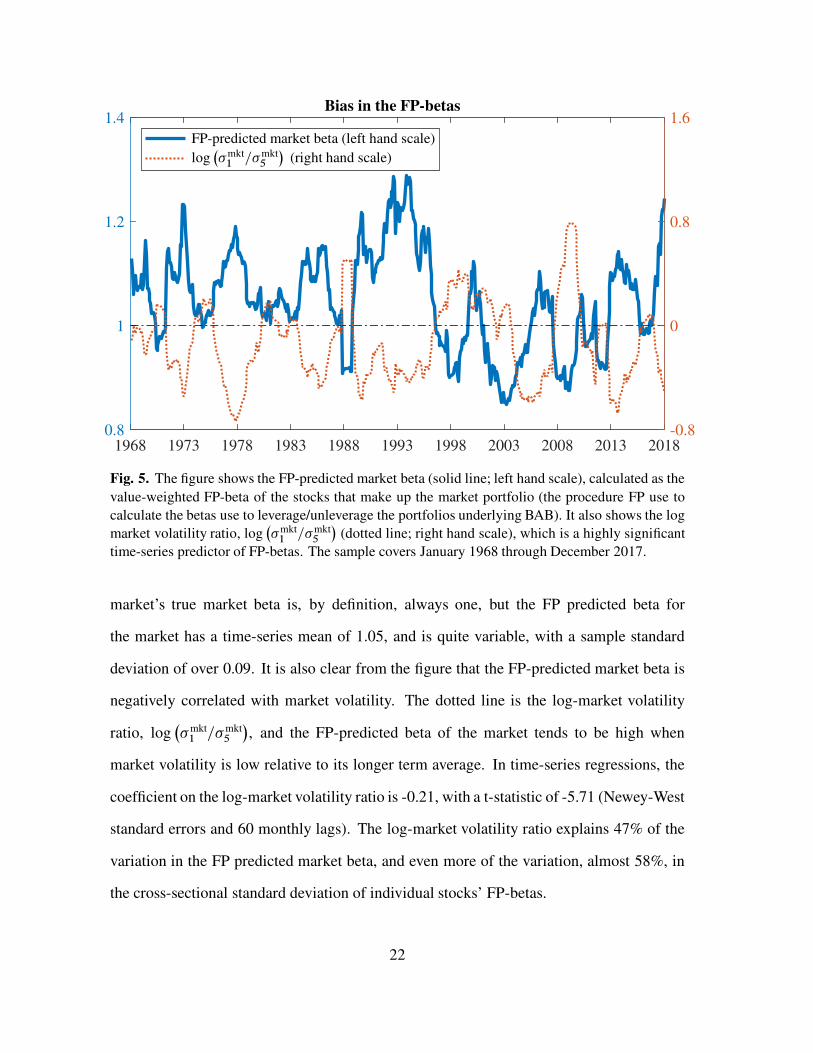
Figure 5 confirms this prediction. The solid line is the value-weighted average FP-beta

for the whole market, i.e., the predicted market beta obtained each month using the

procedure FP use to predict the betas of portfolios underlying BAB.17 Following FP, we

apply shrinkage to individual stock betas, with a 60% weight on the empirical estimate

and a 40% weight on one (i.e., on the true market-weighted average of individual stocks’

market betas).18 The figure shows bias in the beta FP predict for the market. The

16 Because �mkt5 =�mkt

1 is constant within each cross-sectional regression, the average cross-sectional R2 for

this Fama and MacBeth regression is the same 98.3% we observed using ˇi5� i

1=� i5 as the explanatory variable.

17 FP calculate portfolio betas as holdings-weighted averages of the estimated betas of the stocks they hold,

but this is not a valid procedure when using FP-beta; a portfolio’s market beta is the weighted-average beta ofits holdings, but a similar relation does not hold for betas calculated using FP’s non-standard procedure. To

see this, suppose a portfolio holds n stocks with weights given by wi for i 2 f1; 2; :::; ngwherePn

iD1 wi D 1.

Then the portfolio’s FP-beta is

ˇprtFP D

�prt1 =�

prt5

�mkt1 =�mkt

5

!

ˇprt5 D

�prt1 =�

prt5

�mkt1 =�mkt

5

!nX

iD1

wiˇi5 D

nX

iD1

�prt1 =�

prt5

� i1=� i

5

!

wiˇiFP:

This is not equal toPn

iD1 wiˇiFP, the weighted-average FP-beta estimate. Note that this also implies that the

FP-beta of a long/short strategy is not the difference in the FP-betas of the strategy’s long and short sides.18 The shrinkage FP apply to individual stock beta estimates directly impacts BAB’s performance.

Shrinkage does not affect the rank-ordering of beta estimates, so does not change the underlying beta

portfolios, but the degree of shrinkage they use when estimating individual stock betas is directly inherited by

their portfolio beta estimates, and is thus a parameter that directly impacts the leverage employed for hedging.

This problem is avoided when directly estimating portfolio betas using the portfolios’ realized returns.

21

1968 1973 1978 1983 1988 1993 1998 2003 2008 2013 20180.8

1

1.2

1.4

-0.8

0

0.8

1.6Bias in the FP-betas

FP-predicted market beta (left hand scale)

log�

�mkt1 =�mkt

5

�

(right hand scale)

Fig. 5. The figure shows the FP-predicted market beta (solid line; left hand scale), calculated as the

value-weighted FP-beta of the stocks that make up the market portfolio (the procedure FP use to

calculate the betas use to leverage/unleverage the portfolios underlying BAB). It also shows the log

market volatility ratio, log�

�mkt1 =�mkt

5

�

(dotted line; right hand scale), which is a highly significant

time-series predictor of FP-betas. The sample covers January 1968 through December 2017.

market’s true market beta is, by definition, always one, but the FP predicted beta for

the market has a time-series mean of 1.05, and is quite variable, with a sample standard

deviation of over 0.09. It is also clear from the figure that the FP-predicted market beta is

negatively correlated with market volatility. The dotted line is the log-market volatility

ratio, log�

�mkt1 =�mkt

5

�

, and the FP-predicted beta of the market tends to be high when

market volatility is low relative to its longer term average. In time-series regressions, the

coefficient on the log-market volatility ratio is -0.21, with a t-statistic of -5.71 (Newey-West

standard errors and 60 monthly lags). The log-market volatility ratio explains 47% of the

variation in the FP predicted market beta, and even more of the variation, almost 58%, in

the cross-sectional standard deviation of individual stocks’ FP-betas.

22

These facts have profound implications for the interpretation of the empirical evidence

FP provide in support of their paper’s underlying theory. FP argue that their model “predicts

that the betas of securities in the cross section are compressed toward one when funding

liquidity risk is high” and claim to show that “consistent with [FP’s] Proposition 4, the

cross-sectional dispersion in betas is lower when credit constraints are more volatile” (p.

17). In particular, FP argue that TED-spread volatility is a proxy for funding constraints,

and present evidence that beta dispersion, measured by the observed cross-sectional

standard deviation, mean absolute deviation, or interquartile range, is significantly lower

when TED-spread volatility is high. This result is difficult to interpret, however, because

the referenced table does not report dispersion in betas, but dispersion in FP-betas, which,

as discussed above, are strongly biased in predictable ways.

Table 3 evaluates FP’s beta compression claims, contrasting the power that TED-spread

volatility has predicting dispersion in the biased FP-betas to its lack of power predicting the

spread in the high and low beta portfolios’ realized market betas. The first specification of

Panel A mimics FP’s Table 10, investigating the extent to which TED-spread volatility

predicts FP-beta dispersion, measured by ˇHFP � ˇL

FP, the FP-predicted spread between

the high and low beta portfolios underlying BAB.19 Consistent with FP, the prior month’s

realized TED-spread volatility is a negative predictor of FP-beta dispersion, though it is not

statistically significant and explains little of the time-series variation in this dispersion.20

The second specification shows that the level of the TED-spread, which is highly correlated

19 This measure is closely related to FP’s interquartile spread. Appendix E shows similar results using the

standard deviation and mean absolute deviation of individual stocks’ FP-beta estimates.20 Interpretation of this result is further complicated, because FP calculate TED-spread volatility using

another non-standard procedure. Interest rate volatility is commonly measured as the annualized standard

deviation of changes in the log-rate, but FP measure TED-spread volatility each calendar month as the

annualized standard deviation of daily changes in the level of the spread. TED-spread innovations tend to

be proportional to the spread, so this measure of TED-spread volatility (or more accurately, TED-spreadvariability) is highly correlated with the TED-spread. The level of the TED-spread explains 66.5% of the

variation in the TED-spread volatility measure employed by FP, despite explaining none of the variation

(adj.-R2 D 0:0%) in conventionally measured TED-spread volatility. For comparability we follow FP, using

their unconventional measure of TED-spread volatility.

23

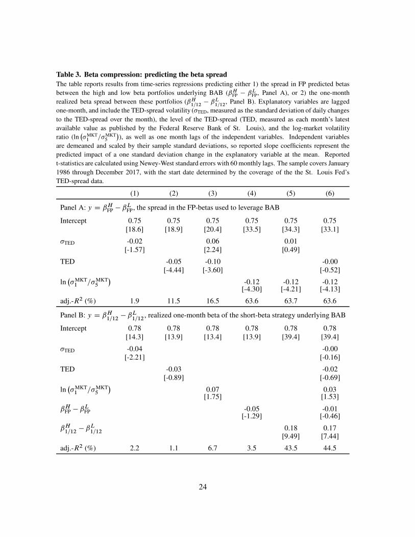
Table 3. Beta compression: predicting the beta spread

The table reports results from time-series regressions predicting either 1) the spread in FP predicted betas

between the high and low beta portfolios underlying BAB (ˇHFP � ˇL

FP, Panel A), or 2) the one-month

realized beta spread between these portfolios (ˇH1=12� ˇL

1=12, Panel B). Explanatory variables are lagged

one-month, and include the TED-spread volatility (�TED, measured as the standard deviation of daily changes

to the TED-spread over the month), the level of the TED-spread (TED, measured as each month’s latest

available value as published by the Federal Reserve Bank of St. Louis), and the log-market volatility

ratio (ln�

�MKT1 =�MKT

5

�

), as well as one month lags of the independent variables. Independent variables

are demeaned and scaled by their sample standard deviations, so reported slope coefficients represent the

predicted impact of a one standard deviation change in the explanatory variable at the mean. Reported

t-statistics are calculated using Newey-West standard errors with 60 monthly lags. The sample covers January

1986 through December 2017, with the start date determined by the coverage of the the St. Louis Fed’s

TED-spread data.

(1) (2) (3) (4) (5) (6)

Panel A: y D ˇHFP � ˇL

FP , the spread in the FP-betas used to leverage BAB

Intercept 0.75 0.75 0.75 0.75 0.75 0.75[18.6] [18.9] [20.4] [33.5] [34.3] [33.1]

�TED -0.02 0.06 0.01[-1.57] [2.24] [0.49]

TED -0.05 -0.10 -0.00[-4.44] [-3.60] [-0.52]

ln�

�MKT1 =�MKT

5

�

-0.12 -0.12 -0.12[-4.30] [-4.21] [-4.13]

adj.-R2 (%) 1.9 11.5 16.5 63.6 63.7 63.6

Panel B: y D ˇH1=12� ˇL

1=12, realized one-month beta of the short-beta strategy underlying BAB

Intercept 0.78 0.78 0.78 0.78 0.78 0.78[14.3] [13.9] [13.4] [13.9] [39.4] [39.4]

�TED -0.04 -0.00[-2.21] [-0.16]

TED -0.03 -0.02[-0.89] [-0.69]

ln�

�MKT1 =�MKT

5

�

0.07 0.03[1.75] [1.53]

ˇHFP � ˇL

FP -0.05 -0.01[-1.29] [-0.46]

ˇH1=12� ˇL

1=120.18 0.17

[9.49] [7.44]

adj.-R2 (%) 2.2 1.1 6.7 3.5 43.5 44.5

24

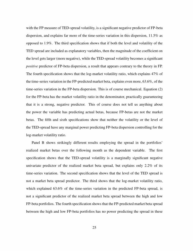
with the FP measure of TED-spread volatility, is a significant negative predictor of FP-beta

dispersion, and explains far more of the time-series variation in this dispersion, 11.5% as

opposed to 1.9%. The third specification shows that if both the level and volatility of the

TED spread are included as explanatory variables, then the magnitude of the coefficient on

the level gets larger (more negative), while the TED-spread volatility becomes a significant

positive predictor of FP-beta dispersion, a result that appears contrary to the theory in FP.

The fourth specification shows that the log-market volatility ratio, which explains 47% of

the time-series variation in the FP-predicted market beta, explains even more, 63.6%, of the

time-series variation in the FP-beta dispersion. This is of course mechanical. Equation (2)

for the FP-beta has the market volatility ratio in the denominator, practically guaranteeing

that it is a strong, negative predictor. This of course does not tell us anything about

the power the variable has predicting actual betas, because FP-betas are not the market

betas. The fifth and sixth specifications show that neither the volatility or the level of

the TED-spread have any marginal power predicting FP-beta dispersion controlling for the

log-market volatility ratio.

Panel B shows strikingly different results employing the spread in the portfolios’

realized market betas over the following month as the dependent variable. The first

specification shows that the TED-spread volatility is a marginally significant negative

univariate predictor of the realized market beta spread, but explains only 2.2% of its

time-series variation. The second specification shows that the level of the TED spread is

not a market beta spread predictor. The third shows that the log-market volatility ratio,

which explained 63.6% of the time-series variation in the predicted FP-beta spread, is

not a significant predictor of the realized market beta spread between the high and low

FP-beta portfolios. The fourth specification shows that the FP-predicted market beta spread

between the high and low FP-beta portfolios has no power predicting the spread in these

25

portfolios’ actual market betas. The last two specifications contrast this with the power that

the lagged realized market beta spread has predicting the market beta spread. Market betas

are persistent, so the portfolios’ realized betas, even the noisy estimates obtained using

a single month of daily returns, have significant power predicting the portfolios’ betas in

the following month. The lagged realized market beta spread is consequently a highly

significant predictor, with a t-statistic exceeding nine, explaining 44% of the time-series

variation in the following month’s realized market beta spread. The last specification shows

that in a multiple regression the power of the past realized market beta spread to predict the

market beta spread is almost undiminished, while controlling for the past spread none of

the other variables have any power.

Overall, Table 3 suggests that the evidence for beta compression FP present as support

for their paper’s underlying theory actually reflects bias in the paper’s betas, driven by

their non-standard beta estimation procedure. Neither funding constraints, nor even the

FP-predicted beta spread between the high and low beta portfolios, have any power

predicting actual dispersion in market betas. The fact that the FP-predicted betas of

the portfolios underlying BAB do not predict the spread between the portfolios’ actual

market betas has strong implications for BAB’s conditional performance. The portfolios’

FP-predicted betas are both highly predictable and the basis of FP’s hedging procedure.

As a result, market volatility predicts the leverage BAB employs, but not the betas of the

underlying portfolios, so BAB is mis-hedged in predictable ways. As a result, BAB is not

conditionally market-neutral, and market volatility is a powerful predictor of BAB’s market

tilt.21 This fact is further investigated in the next section.

21 FP also predict BAB’s market tilt can be predicted, but for a very different reason. The FP-betas used

to hedge BAB are highly predictable, but the market betas of the portfolios underlying BAB are not. Failingto understand the bias in their betas, FP argue that the market betas of the portfolios underlying BAB can be

predicted using information about TED-spread volatility, which they argue is not incorporated into BAB’s

hedge.

26

5. BAB’s beta

BAB dramatically over-weights nano- and micro-cap stocks (section 3), and the

FP-betas used to create and leverage BAB’s underlying portfolios are biased in highly

predictable ways (section 4). Both these facts raise concerns regarding whether BAB is

truly market-neutral, as it is designed to be.

First, the small stocks disproportionately traded by BAB are prone to asynchronous

trading problems.22 The strategy is significantly net-long these nano- and micro-cap stocks,

to the tune of 70 cents for each dollar invested in BAB. There is also a strong reason to

suspect that the stocks held on the long side of the strategy are especially susceptible to

this issue. These stocks are selected on the basis of having low estimated market betas,

and asynchronous trading problems bias beta estimations downward.23 Because BAB is

significantly net-long nano- and micro-cap stocks, selecting especially for those with the

largest asynchronous trading problems, we should expect that the strategy’s market beta

estimated at longer horizons exceeds its beta estimated at shorter horizons. Given that the

strategy is designed to target a contemporaneous monthly market beta of zero, we should

consequently expect the strategy to have a positive market tilt at longer horizons.

Second, given that the log-market volatility ratio explains 63.6% of the time-series

variation in the FP-predicted beta spread between the high and low beta portfolios, and that

these portfolios’ FP-predicted betas are used to leverage these portfolios when constructing

BAB, we should expect this ratio to also predict BAB’s beta. When volatility is high,

22 FP-betas are calculated using correlations estimated using three-day overlapping returns, a choice made

explicitly to “control for nonsynchronous trading.” The three day window is insufficient to resolve the

problem, especially for the small stocks disproportionately traded by BAB.23 Baker, Taliaferro, and Burnham (2017) adopt the FP beta estimation procedure, calling them “improved

measures of beta,” despite seeming to recognize that doing so “has the effect of lowering the average betasof small stocks, which are individually less likely to trade in sync with the market overall, because of lower

levels of liquidity” (p. 77).

27

then the downward bias in the FP-betas should artificially compress the spread in the

betas used to leverage the portfolios underlying BAB, resulting in under-hedging that is

insufficient to fully offset the underlying low beta-minus-high beta strategy’s short market

tilt. Conversely, when volatility is low the bias should exaggerate the hedging beta spread,

resulting in over-hedging and a long market tilt.

Table 4 tests both these sets of predictions, by performing a series of time-series

regressions of the returns to BAB on the contemporaneous market return, lagged market

returns, and market returns interacted with the log of the one year to five year market

volatility ratio. The first specification shows that BAB is close to contemporaneously

market-neutral at the monthly frequency, with an average loading on the market of -0.06

that is barely significant (t-statistic of -1.98). The second specification includes one- and

two-month lagged market returns as explanatory variables, and finds these to be much better

predictors of BAB’s performance. The loadings are larger, 0.16 and 0.11 respectively,

and highly significant (t-statistics of 5.96 and 3.60), suggesting that BAB has a significant

long market tilt at lower frequencies, a fact also reflected in the data—the market beta of

BAB in annual data is 0.29. This fact also helps explain the striking difference in betas

observed on the daily and monthly BAB factors maintained by AQR. The monthly factor,

like our replication, has a -0.06 contemporaneous beta in the post-1967 sample (t-statistic of

-2.28). The magnitude of the short market tilt measured at the daily frequency, however, is

significantly larger, -0.33 (t-statistic of -14.8 using Newey-West standard errors calculated

with one month of daily lags), despite the fact that this daily factor’s cumulated returns

each month closely match the returns to the monthly factor. Understanding the magnitude

of the non-synchronous trading issues that plague BAB helps reconcile these seemingly

disparate results.

The third specification explores BAB’s conditional market tilt, by additionally including

28

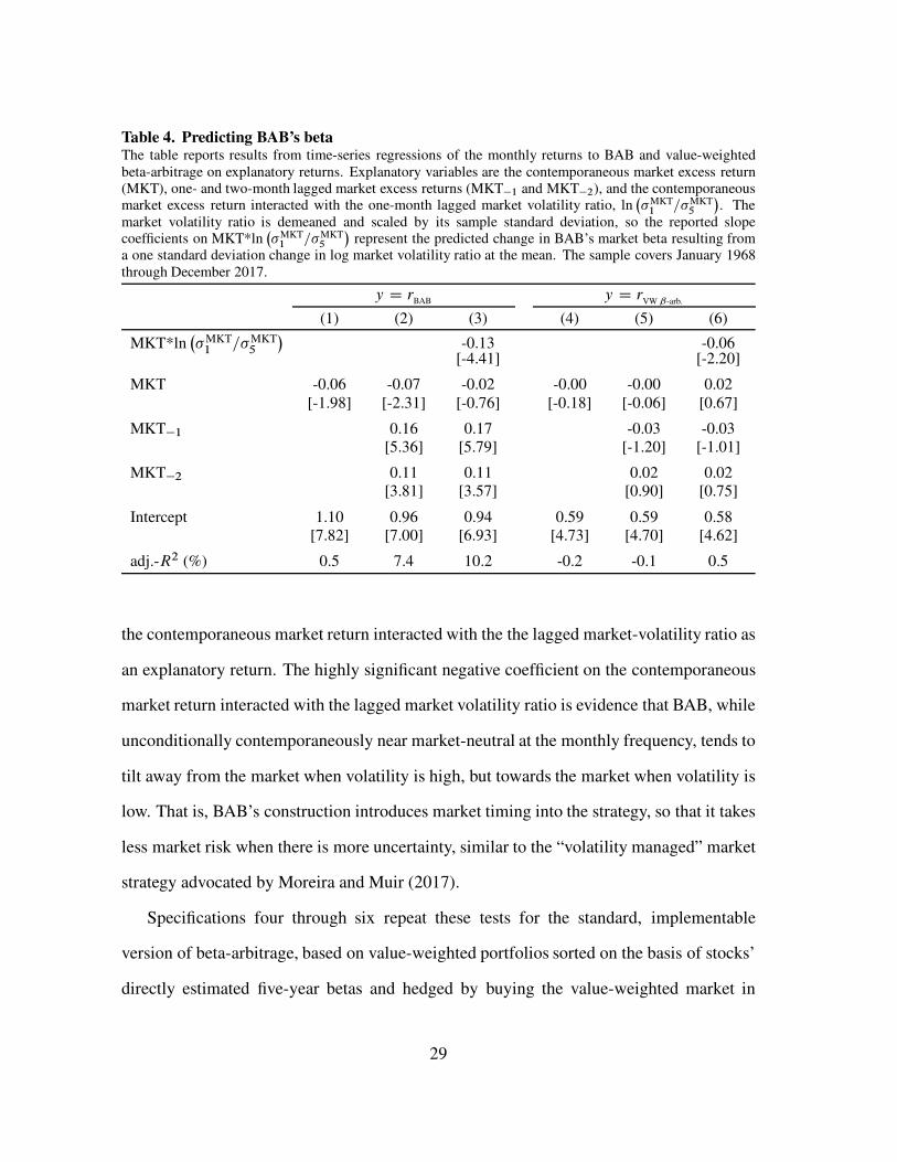
Table 4. Predicting BAB’s betaThe table reports results from time-series regressions of the monthly returns to BAB and value-weightedbeta-arbitrage on explanatory returns. Explanatory variables are the contemporaneous market excess return(MKT), one- and two-month lagged market excess returns (MKT�1 and MKT�2), and the contemporaneousmarket excess return interacted with the one-month lagged market volatility ratio, ln

�

�MKT1 =�MKT

5

�

. Themarket volatility ratio is demeaned and scaled by its sample standard deviation, so the reported slopecoefficients on MKT*ln

�

�MKT1 =�MKT

5

�

represent the predicted change in BAB’s market beta resulting froma one standard deviation change in log market volatility ratio at the mean. The sample covers January 1968through December 2017.

y D rBAB

y D rVW ˇ-arb.

(1) (2) (3) (4) (5) (6)

MKT*ln�

�MKT1 =�MKT

5

�

-0.13 -0.06[-4.41] [-2.20]

MKT -0.06 -0.07 -0.02 -0.00 -0.00 0.02[-1.98] [-2.31] [-0.76] [-0.18] [-0.06] [0.67]

MKT�1 0.16 0.17 -0.03 -0.03[5.36] [5.79] [-1.20] [-1.01]

MKT�2 0.11 0.11 0.02 0.02[3.81] [3.57] [0.90] [0.75]

Intercept 1.10 0.96 0.94 0.59 0.59 0.58[7.82] [7.00] [6.93] [4.73] [4.70] [4.62]

adj.-R2 (%) 0.5 7.4 10.2 -0.2 -0.1 0.5

the contemporaneous market return interacted with the the lagged market-volatility ratio as

an explanatory return. The highly significant negative coefficient on the contemporaneous

market return interacted with the lagged market volatility ratio is evidence that BAB, while

unconditionally contemporaneously near market-neutral at the monthly frequency, tends to

tilt away from the market when volatility is high, but towards the market when volatility is

low. That is, BAB’s construction introduces market timing into the strategy, so that it takes

less market risk when there is more uncertainty, similar to the “volatility managed” market

strategy advocated by Moreira and Muir (2017).

Specifications four through six repeat these tests for the standard, implementable

version of beta-arbitrage, based on value-weighted portfolios sorted on the basis of stocks’

directly estimated five-year betas and hedged by buying the value-weighted market in

29

proportion to the underlying low beta-minus-high beta strategy’s observed market tilt

over the preceding year. These tests show that the non-synchronous trading issues that

plague BAB are absent from this beta-arbitrage. Beta-arbitrage is contemporaneously

market-neutral (specification 4), and also market-neutral at longer horizons (specification

5). The last specification shows, consistent with the results of Cederburg and O’Doherty

(2016), that beta-arbitrage, like BAB, has a degree of volatility-related market timing,

though the magnitude is less than half as large.

6. Conclusion

Frazzini and Pedersen’s (2014) Betting Against Beta (BAB) factor, based on

the same basic idea as Black’s (1972) beta-arbitrage, exhibits striking backtested

performance. This remarkable performance depends, however, on non-standard choices

FP make when constructing BAB. Their rank-weighting procedure is a backdoor to

equal-weighing the strategy’s underlying beta portfolios, and their leveraging procedure

is a backdoor to hedging the underlying low beta-minus-high beta portfolio using these

same portfolios. The resulting strategy, BAB, is little different from a simple, transparent

version of beta-arbitrage, based on equal-weighted beta portfolios and hedged using the

equal-weighted market. While this fact is obscured by FP’s non-standard construction

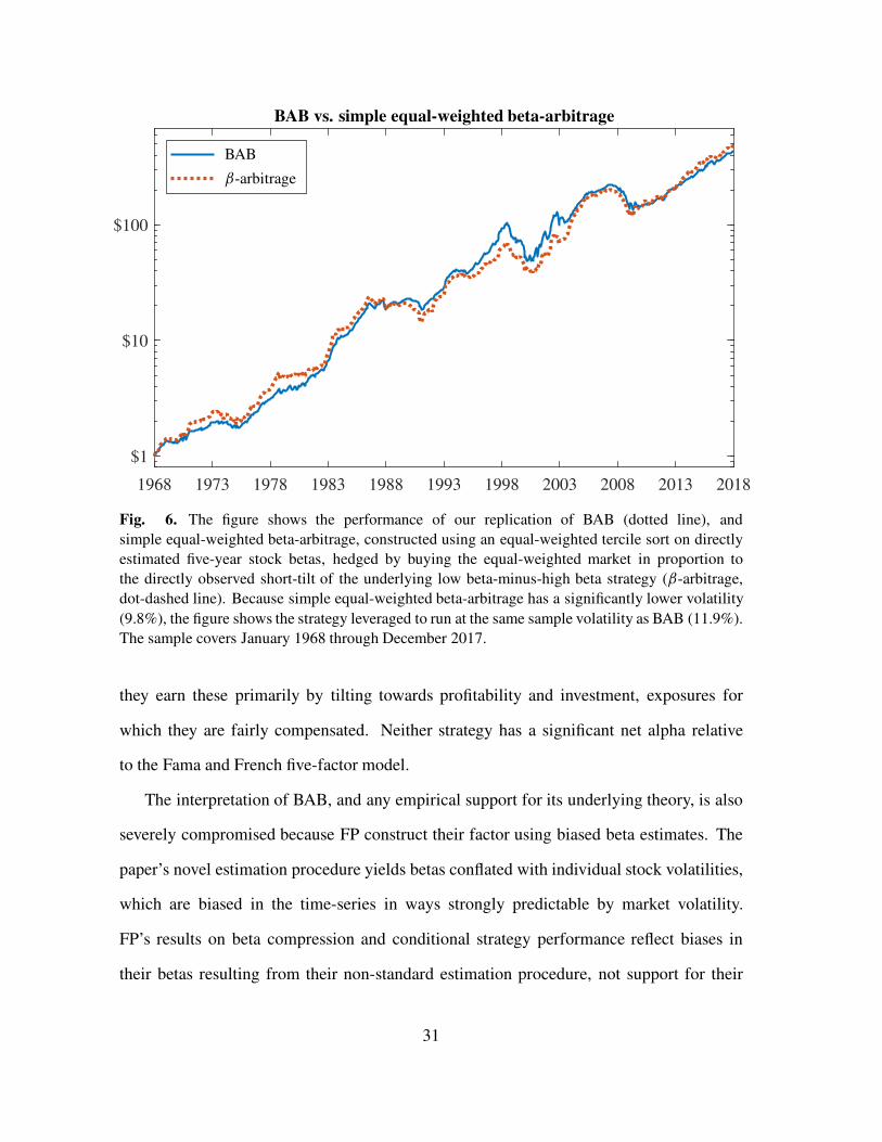
methods, it is readily apparent in Figure 6, which shows the two strategies. The two are

84% correlated, and realize almost identical Sharpe ratios (1.08 for BAB and 1.09 for

beta-arbitrage).

The strong paper performance of both strategies is driven by dramatically

overweighting the market’s smallest, least liquid stocks, while ignoring transaction costs

and implementation issues. Accounting for transaction costs significantly reduces the

strategies’ profitability. While both strategies earn significantly positive average net returns,

30

1968 1973 1978 1983 1988 1993 1998 2003 2008 2013 2018

$1

$10

$100

BAB vs. simple equal-weighted beta-arbitrage

BAB

ˇ-arbitrage

Fig. 6. The figure shows the performance of our replication of BAB (dotted line), and

simple equal-weighted beta-arbitrage, constructed using an equal-weighted tercile sort on directly

estimated five-year stock betas, hedged by buying the equal-weighted market in proportion to

the directly observed short-tilt of the underlying low beta-minus-high beta strategy (ˇ-arbitrage,

dot-dashed line). Because simple equal-weighted beta-arbitrage has a significantly lower volatility

(9.8%), the figure shows the strategy leveraged to run at the same sample volatility as BAB (11.9%).

The sample covers January 1968 through December 2017.

they earn these primarily by tilting towards profitability and investment, exposures for

which they are fairly compensated. Neither strategy has a significant net alpha relative

to the Fama and French five-factor model.

The interpretation of BAB, and any empirical support for its underlying theory, is also

severely compromised because FP construct their factor using biased beta estimates. The

paper’s novel estimation procedure yields betas conflated with individual stock volatilities,

which are biased in the time-series in ways strongly predictable by market volatility.

FP’s results on beta compression and conditional strategy performance reflect biases in

their betas resulting from their non-standard estimation procedure, not support for their

31

underlying theory.

Overall, the results presented in BAB do not provide strong evidence for the profitability

of defensive equity strategies.24 Instead, they provide a powerful argument against the use

of “sophisticated” or non-standard procedures. While novel techniques certainly have a

role in economics, and are sometimes necessary to advance our knowledge, they are too

often used to make results look stronger without yielding any deeper insights.

This provides a compelling rationale for “following the literature.” No matter how

arbitrary the choices made by the previous literature, they are past choices, and following

them now reduces the degrees of freedom available for overfitting the data when doing

empirical research (see also Novy-Marx 2018). As a consequence, deviations from

well-accepted methods should be both well motivated and well understood. When results

are obtained using non-standard methods, the first question should be “What are the results

using standard methods?” If the answer is “different, but those obtained using non-standard

methods are still interesting,” the next question should be “Why? And what, exactly, is

driving any differences?” When a non-standard method’s impact on results is not obvious,

or the mechanism driving any difference is not clear, its real impact may well be different

than you think, and different from what is claimed.

24 Novy-Marx (2016) also shows that the performance of “defensive” strategies that bet against volatility

can be understood by the tilts they take to profitability and value, at least after controlling for size.

32

A. Appendix: Comparison of BAB factors

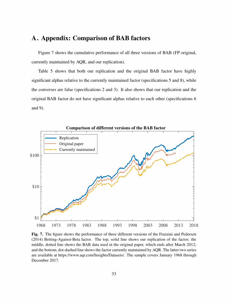
Figure 7 shows the cumulative performance of all three versions of BAB (FP original,

currently maintained by AQR, and our replication).

Table 5 shows that both our replication and the original BAB factor have highly

significant alphas relative to the currently maintained factor (specifications 5 and 8), while

the converses are false (specifications 2 and 3). It also shows that our replication and the

original BAB factor do not have significant alphas relative to each other (specifications 6

and 9).

1968 1973 1978 1983 1988 1993 1998 2003 2008 2013 2018

$1

$10

$100

Comparison of different versions of the BAB factor

Replication

Original paper

Currently maintained

Fig. 7. The figure shows the performance of three different versions of the Frazzini and Pedersen

(2014) Betting-Against-Beta factor. The top, solid line shows our replication of the factor; the

middle, dotted line shows the BAB data used in the original paper, which ends after March 2012;

and the bottom, dot-dashed line shows the factor currently maintained by AQR. The latter two series

are available at https://www.aqr.com/Insights/Datasets/. The sample covers January 1968 through

December 2017.

33

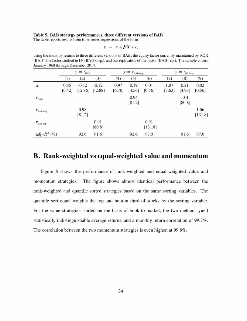
Table 5. BAB strategy performances, three different versions of BABThe table reports results from time-series regressions of the form

y D ˛ C ˇ 0XC �;

using the monthly returns to three different versions of BAB: the equity factor currently maintained by AQR

(BAB), the factor studied in FP (BAB-orig.), and our replication of the factor (BAB-rep.). The sample covers

January 1968 through December 2017.

y D rBAB

y D rBAB-orig.

y D rBAB-rep.

(1) (2) (3) (4) (5) (6) (7) (8) (9)

˛ 0.85 -0.12 -0.12 0.97 0.19 0.01 1.07 0.21 0.02[6.42] [-2.86] [-2.88] [6.70] [4.56] [0.56] [7.63] [4.93] [0.56]

rBAB

0.94 1.01[81.2] [80.8]

rBAB-orig.

0.98 1.06[81.2] [131.8]

rBAB-rep.

0.91 0.91[80.8] [131.8]

adj.-R2 (%) 92.6 91.6 92.6 97.0 91.6 97.0

B. Rank-weighted vs equal-weighted value and momentum

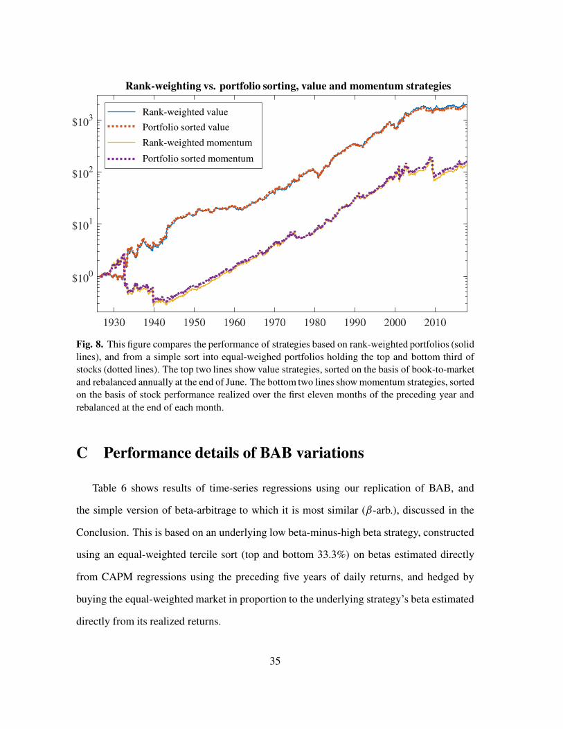
Figure 8 shows the performance of rank-weighted and equal-weighted value and

momentum strategies. The figure shows almost identical performance between the

rank-weighted and quantile sorted strategies based on the same sorting variables. The

quantile sort equal weights the top and bottom third of stocks by the sorting variable.

For the value strategies, sorted on the basis of book-to-market, the two methods yield

statistically indistinguishable average returns, and a monthly return correlation of 99.7%.

The correlation between the two momentum strategies is even higher, at 99.8%.

34

1930 1940 1950 1960 1970 1980 1990 2000 2010

$100

$101

$102

$103

Rank-weighting vs. portfolio sorting, value and momentum strategies

Rank-weighted value

Portfolio sorted value

Rank-weighted momentum

Portfolio sorted momentum

Fig. 8. This figure compares the performance of strategies based on rank-weighted portfolios (solid

lines), and from a simple sort into equal-weighed portfolios holding the top and bottom third of

stocks (dotted lines). The top two lines show value strategies, sorted on the basis of book-to-market

and rebalanced annually at the end of June. The bottom two lines show momentum strategies, sorted

on the basis of stock performance realized over the first eleven months of the preceding year and

rebalanced at the end of each month.

C Performance details of BAB variations

Table 6 shows results of time-series regressions using our replication of BAB, and

the simple version of beta-arbitrage to which it is most similar (ˇ-arb.), discussed in the

Conclusion. This is based on an underlying low beta-minus-high beta strategy, constructed

using an equal-weighted tercile sort (top and bottom 33.3%) on betas estimated directly

from CAPM regressions using the preceding five years of daily returns, and hedged by

buying the equal-weighted market in proportion to the underlying strategy’s beta estimated

directly from its realized returns.

35

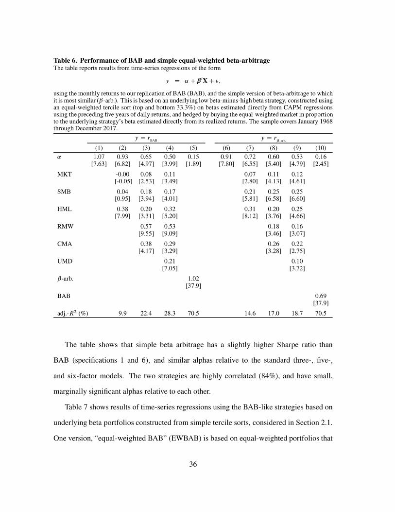
Table 6. Performance of BAB and simple equal-weighted beta-arbitrageThe table reports results from time-series regressions of the form

y D ˛ C ˇ 0XC �;

using the monthly returns to our replication of BAB (BAB), and the simple version of beta-arbitrage to whichit is most similar (ˇ-arb.). This is based on an underlying low beta-minus-high beta strategy, constructed usingan equal-weighted tercile sort (top and bottom 33.3%) on betas estimated directly from CAPM regressionsusing the preceding five years of daily returns, and hedged by buying the equal-weighted market in proportionto the underlying strategy’s beta estimated directly from its realized returns. The sample covers January 1968through December 2017.

y D rBAB

y D rˇ-arb.

(1) (2) (3) (4) (5) (6) (7) (8) (9) (10)

˛ 1.07 0.93 0.65 0.50 0.15 0.91 0.72 0.60 0.53 0.16[7.63] [6.82] [4.97] [3.99] [1.89] [7.80] [6.55] [5.40] [4.79] [2.45]

MKT -0.00 0.08 0.11 0.07 0.11 0.12[-0.05] [2.53] [3.49] [2.80] [4.13] [4.61]

SMB 0.04 0.18 0.17 0.21 0.25 0.25[0.95] [3.94] [4.01] [5.81] [6.58] [6.60]

HML 0.38 0.20 0.32 0.31 0.20 0.25[7.99] [3.31] [5.20] [8.12] [3.76] [4.66]

RMW 0.57 0.53 0.18 0.16[9.55] [9.09] [3.46] [3.07]

CMA 0.38 0.29 0.26 0.22[4.17] [3.29] [3.28] [2.75]

UMD 0.21 0.10[7.05] [3.72]

ˇ-arb. 1.02[37.9]

BAB 0.69[37.9]

adj.-R2 (%) 9.9 22.4 28.3 70.5 14.6 17.0 18.7 70.5

The table shows that simple beta arbitrage has a slightly higher Sharpe ratio than

BAB (specifications 1 and 6), and similar alphas relative to the standard three-, five-,

and six-factor models. The two strategies are highly correlated (84%), and have small,

marginally significant alphas relative to each other.

Table 7 shows results of time-series regressions using the BAB-like strategies based on

underlying beta portfolios constructed from simple tercile sorts, considered in Section 2.1.

One version, “equal-weighted BAB” (EWBAB) is based on equal-weighted portfolios that

36

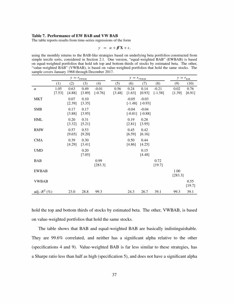
Table 7. Performance of EW BAB and VW BABThe table reports results from time-series regressions of the form

y D ˛ C ˇ 0XC �;

using the monthly returns to the BAB-like strategies based on underlying beta portfolios constructed fromsimple tercile sorts, considered in Section 2.1. One version, “equal-weighted BAB” (EWBAB) is basedon equal-weighted portfolios that hold teh top and bottom thirds of stocks by estimated beta. The other,“value-weighted BAB” (VWBAB), is based on value-weighted portfolios that hold the same stocks. Thesample covers January 1968 through December 2017.

y D rEWBAB y D rVWBAB y D rBAB

(1) (2) (3) (4) (5) (6) (7) (8) (9) (10)

˛ 1.05 0.63 0.49 -0.01 0.56 0.24 0.14 -0.21 0.02 0.76[7.53] [4.88] [3.89] [-0.76] [3.48] [1.63] [0.93] [-1.58] [1.39] [6.91]

MKT 0.07 0.10 -0.05 -0.03[2.39] [3.35] [-1.48] [-0.93]

SMB 0.17 0.17 -0.04 -0.04[3.88] [3.95] [-0.81] [-0.88]

HML 0.20 0.31 0.19 0.28[3.32] [5.21] [2.81] [3.95]

RMW 0.57 0.53 0.45 0.42[9.65] [9.20] [6.59] [6.16]

CMA 0.39 0.30 0.50 0.44[4.29] [3.41] [4.86] [4.25]

UMD 0.20 0.15[7.05] [4.48]

BAB 0.99 0.72[283.3] [19.7]

EWBAB 1.00[283.3]

VWBAB 0.55[19.7]

adj.-R2 (%) 23.0 28.8 99.3 24.3 26.7 39.1 99.3 39.1

hold the top and bottom thirds of stocks by estimated beta. The other, VWBAB, is based

on value-weighted portfolios that hold the same stocks.

The table shows that BAB and equal-weighted BAB are basically indistinguishable.

They are 99.6% correlated, and neither has a significant alpha relative to the other

(specifications 4 and 9). Value-weighted BAB is far less similar to these strategies, has

a Sharpe ratio less than half as high (specification 5), and does not have a significant alpha

37

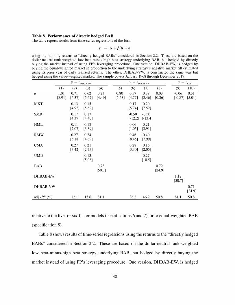
Table 8. Performance of directly hedged BABThe table reports results from time-series regressions of the form

y D ˛ C ˇ 0XC �;

using the monthly returns to “directly hedged BABs” considered in Section 2.2. These are based on thedollar-neutral rank-weighted low beta-minus-high beta strategy underlying BAB, but hedged by directlybuying the market instead of using FP’s leveraging procedure. One version, DHBAB-EW, is hedged bybuying the equal-weighted market in proportion to the underlying strategy’s negative market tilt estimatedusing its prior year of daily realized returns. The other, DHBAB-VW, is constructed the same way buthedged using the value-weighted market. The sample covers January 1968 through December 2017.

y D rDHBAB-EW

y D rDHBAB-VW

y D rBAB

(1) (2) (3) (4) (5) (6) (7) (8) (9) (10)

˛ 1.01 0.71 0.62 0.23 0.80 0.57 0.38 0.03 -0.06 0.51[8.91] [6.37] [5.62] [4.49] [5.63] [4.77] [3.46] [0.26] [-0.87] [5.01]

MKT 0.13 0.15 0.17 0.20[4.92] [5.62] [5.74] [7.52]

SMB 0.17 0.17 -0.50 -0.50[4.37] [4.40] [-12.2] [-13.4]

HML 0.11 0.18 0.06 0.21[2.07] [3.39] [1.05] [3.91]

RMW 0.27 0.24 0.46 0.40[5.18] [4.69] [8.45] [7.99]

CMA 0.27 0.21 0.28 0.16[3.42] [2.73] [3.30] [2.05]

UMD 0.13 0.27[5.08] [10.5]

BAB 0.73 0.72[50.7] [24.9]

DHBAB-EW 1.12[50.7]

DHBAB-VW 0.71[24.9]

adj.-R2 (%) 12.1 15.6 81.1 36.2 46.2 50.8 81.1 50.8

relative to the five- or six-factor models (specifications 6 and 7), or to equal-weighted BAB

(specification 8).

Table 8 shows results of time-series regressions using the returns to the “directly hedged

BABs” considered in Section 2.2. These are based on the dollar-neutral rank-weighted

low beta-minus-high beta strategy underlying BAB, but hedged by directly buying the

market instead of using FP’s leveraging procedure. One version, DHBAB-EW, is hedged

38

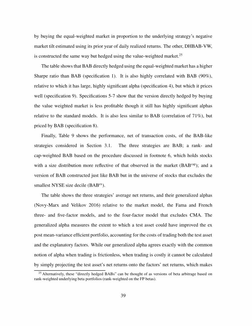
by buying the equal-weighted market in proportion to the underlying strategy’s negative

market tilt estimated using its prior year of daily realized returns. The other, DHBAB-VW,

is constructed the same way but hedged using the value-weighted market.25

The table shows that BAB directly hedged using the equal-weighted market has a higher

Sharpe ratio than BAB (specification 1). It is also highly correlated with BAB (90%),

relative to which it has large, highly significant alpha (specification 4), but which it prices

well (specification 9). Specifications 5-7 show that the version directly hedged by buying

the value weighted market is less profitable though it still has highly significant alphas

relative to the standard models. It is also less similar to BAB (correlation of 71%), but

priced by BAB (specification 8).

Finally, Table 9 shows the performance, net of transaction costs, of the BAB-like

strategies considered in Section 3.1. The three strategies are BAB; a rank- and

cap-weighted BAB based on the procedure discussed in footnote 6, which holds stocks

with a size distribution more reflective of that observed in the market (BABcap); and a

version of BAB constructed just like BAB but in the universe of stocks that excludes the

smallest NYSE size decile (BABex).

The table shows the three strategies’ average net returns, and their generalized alphas

(Novy-Marx and Velikov 2016) relative to the market model, the Fama and French

three- and five-factor models, and to the four-factor model that excludes CMA. The

generalized alpha measures the extent to which a test asset could have improved the ex

post mean-variance efficient portfolio, accounting for the costs of trading both the test asset

and the explanatory factors. While our generalized alpha agrees exactly with the common

notion of alpha when trading is frictionless, when trading is costly it cannot be calculated

by simply projecting the test asset’s net returns onto the factors’ net returns, which makes

25 Alternatively, these “directly hedged BABs” can be thought of as versions of beta arbitrage based on

rank-weighted underlying beta portfolios (rank-weighted on the FP betas).

39

Table 9. BAB performance net of transaction costsThe table reports the performance of BAB net of transaction costs using the generalized alpha of Novy-Marxand Velikov (2016), which measures the extent to which adding a test asset improves the investmentopportunity set relative to a set of explanatory factors accounting for the cost of trading. In addition to BAB,it reports results for rank- and capitalization-weighted BAB (BABcap), and for BAB constructed in a universethat excludes the nano-cap stocks from the smallest NYSE size decile (BABex). The table also reports theweight of each asset in the achievable (net of transaction costs) ex post MVE portfolio. The sample coversJanuary 1968 through December 2017.

Factor weight in ex post MVE portfolio

Test asset Explanatory factors

˛� BAB BABcap BABex MKT SMB HML RMW CMA SR

Panel A: No model (average net returns)

0.48 1.00 0.47

[3.30]

0.43 1.00 0.39[2.75]

0.47 1.00 0.48[3.37]

Panel B: One-factor model 1.00 0.40

0.51 0.59 0.41 0.64[3.52]

0.54 0.54 0.46 0.65[3.61]

0.55 0.60 0.40 0.69[3.94]

Panel C: Three-factor model 0.38 0.05 0.56 0.63

0.34 0.29 0.32 0.04 0.35 0.72[2.45]

0.34 0.27 0.33 0.09 0.31 0.73[2.47]

0.34 0.33 0.31 0.09 0.28 0.75[2.74]

Panel D: Four-factor model 0.21 0.14 0.27 0.38 0.80

0.20 0.11 0.21 0.12 0.23 0.33 0.83[1.50]

0.25 0.12 0.21 0.14 0.20 0.33 0.84[1.82]

0.17 0.13 0.21 0.14 0.21 0.31 0.83[1.51]

Panel E: Five-factor model 0.17 0.08 0 0.34 0.40 0.95

0.16 0.06 0.17 0.08 0 0.31 0.38 0.96[1.20]

0.19 0.06 0.18 0.09 0 0.31 0.36 0.97[1.36]

0.15 0.07 0.17 0.09 0 0.30 0.37 0.96[1.23]

40

the test asset’s factor loadings uninformative. Consequently, to provide a sense of how

the test assets improve the investment opportunity set relative to each factor model, the

table reports ex post mean variance efficient tangency portfolio weights and the maximum

attainable Sharpe ratios, accounting for transaction costs.

Panel A shows that the three strategies realized remarkably similar average net returns,

43-48 bps/month, and similar Sharpe ratios. They did so despite having highly disparate

costs of trading, ranging from only 8 bps/month for rank- and cap-weighted BAB to almost

60 bps/month for BAB (over the last ten years of the sample these costs were only 5 and 26

bps/month, respectively; the cost of trading BAB ex-nanos lies in between, at 23 bps/month

over the whole sample, and 12 bps/month over the late sample). The strategies’ generalized

alphas relative to the five-factor model (Panel E) are similarly close, ranging from 16 to 19

bps/month, with t-statistics ranging from 1.20 to 1.36. An investor already trading the five

Fama and French factors could not in practice have realized significant gains by additionally

trading any of these versions of BAB (maximal Sharpe ratio improvements from 0.95 to

0.96-0.97), and the ex post efficient portfolio of the factors plus any of the versions of BAB

takes only a modest position in BAB (6-7% of the portfolio).26

26 Panel C shows that all three versions of BAB are correlated with value (35-48%), observable in the

weight reduction on HML in the ex post efficient portfolio that results from adding BAB to the investmentopportunity set (reductions from 0.56 down to 0.28-0.35), but that all three BABs have significant generalized

alphas relative to the three-factor model (34 bps/month with t-statistics ranging from 2.45 to 2.74). Panel D

shows that adding profitability to the set of explanatory factors makes all three BAB strategies’ generalized

alphas insignificant. With these four factors, the weight put on the BABs (0.11-0.13) in the ex post efficient

portfolios is pulled fairly equally from both value and profitability, indicating that it is correlated with boththese factors (35-48% with HML and 29-44% with RMW), but does not significantly improve the opportunity

of an investor already trading the two. In Panel E CMA pushes HML out of the ex post efficient portfolios.

CMA is a good substitute for HML, because they are highly correlated (68%) and have similar Sharpe ratio,

and investment is more complementary to operating profitability than is value: the correlation between CMA

and RMW is -12%, while the correlation between HML and RMW is 17%.

41

D Non-standard FP-betas’ impact on BAB performance

In addition to the time-series bias, using FP-betas instead of market betas has a second

potential effect on the average performance of BAB. In the cross-section, the scaling of

the FP-betas by the market volatility ratio in equation (2) is unimportant, because it is a

multiplier on all the estimates. Sorting on the FP-beta is, however, equivalent to sorting on

the product of 1) stocks’ directly estimated five-year betas, ˇi5, and 2) the ratio of individual

stocks’ volatilities estimated at one and five year horizons, � i1=� i

5. Overall this suggests

two potential effects of the FP-beta estimation procedure on BAB’s average performance,

one driven by stock selection, because cross-sectionally stocks are ranked on the basis of a

combination of their five-year betas and their current volatilities relative to their longer term

means, ˇi5� i

1=� i5, and one driven by the leveraging procedure, because the FP-beta estimates

have a procyclical bias in the time-series, at least to the extent that market volatility is

countercyclical.

Figure 9 shows that the net impact of the two effects on BAB’s average performance

is negligible. In particular, it shows an “almost BAB” strategy, constructed like BAB

but which rank-weights and leverages the underlying portfolios on the basis of directly

estimated five year betas instead of the FP-betas, performs almost indistinguishably from

BAB. The two strategies have monthly return series that are 94.6% correlated, and realize

the same 1.07 Sharpe ratio over the sample peroiod. There is also no advantage, from an

investment perspective, to trading either strategy; neither has a significant alpha relative to

the other, either alone or including the returns to the most common asset pricing factors

(Fama-French five plus UMD) as explanatory returns.

Untabulated results show that BAB has a small but significant alpha (11 bps/month with

a t-statistic of 2.43) relative to a BAB-like strategy based on beta portfolios rank-weighted

42

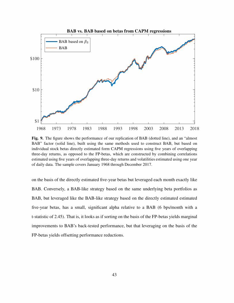
1968 1973 1978 1983 1988 1993 1998 2003 2008 2013 2018

$1

$10

$100

BAB vs. BAB based on betas from CAPM regressions

BAB based on ˇ5

BAB

Fig. 9. The figure shows the performance of our replication of BAB (dotted line), and an “almost

BAB” factor (solid line), built using the same methods used to construct BAB, but based on

individual stock betas directly estimated form CAPM regressions using five years of overlapping

three-day returns, as opposed to the FP-betas, which are constructed by combining correlations

estimated using five years of overlapping three-day returns and volatilities estimated using one year

of daily data. The sample covers January 1968 through December 2017.

on the basis of the directly estimated five-year betas but leveraged each month exactly like

BAB. Conversely, a BAB-like strategy based on the same underlying beta portfolios as

BAB, but leveraged like the BAB-like strategy based on the directly estimated estimated

five-year betas, has a small, significant alpha relative to a BAB (6 bps/month with a

t-statistic of 2.45). That is, it looks as if sorting on the basis of the FP-betas yields marginal

improvements to BAB’s back-tested performance, but that leveraging on the basis of the

FP-betas yields offsetting performance reductions.

43

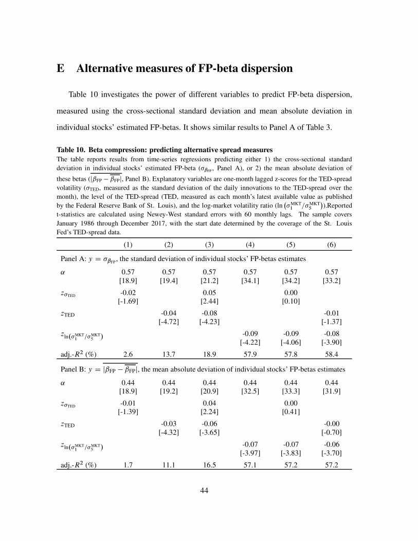
E Alternative measures of FP-beta dispersion

Table 10 investigates the power of different variables to predict FP-beta dispersion,

measured using the cross-sectional standard deviation and mean absolute deviation in

individual stocks’ estimated FP-betas. It shows similar results to Panel A of Table 3.

Table 10. Beta compression: predicting alternative spread measures

The table reports results from time-series regressions predicting either 1) the cross-sectional standard

deviation in individual stocks’ estimated FP-beta (�ˇFP, Panel A), or 2) the mean absolute deviation of

these betas (jˇFP � ˇFPj, Panel B). Explanatory variables are one-month lagged z-scores for the TED-spread

volatility (�TED, measured as the standard deviation of the daily innovations to the TED-spread over the

month), the level of the TED-spread (TED, measured as each month’s latest available value as published

by the Federal Reserve Bank of St. Louis), and the log-market volatility ratio (ln�

�MKT1 =�MKT

5

�

).Reported

t-statistics are calculated using Newey-West standard errors with 60 monthly lags. The sample covers

January 1986 through December 2017, with the start date determined by the coverage of the St. Louis

Fed’s TED-spread data.

(1) (2) (3) (4) (5) (6)

Panel A: y D �ˇFP, the standard deviation of individual stocks’ FP-betas estimates

˛ 0.57 0.57 0.57 0.57 0.57 0.57[18.9] [19.4] [21.2] [34.1] [34.2] [33.2]

z�TED-0.02 0.05 0.00

[-1.69] [2.44] [0.10]

zTED -0.04 -0.08 -0.01[-4.72] [-4.23] [-1.37]

zln.�MKT1

=�MKT5 / -0.09 -0.09 -0.08

[-4.22] [-4.06] [-3.90]

adj.-R2 (%) 2.6 13.7 18.9 57.9 57.8 58.4

Panel B: y D jˇFP � ˇFPj, the mean absolute deviation of individual stocks’ FP-betas estimates

˛ 0.44 0.44 0.44 0.44 0.44 0.44[18.9] [19.2] [20.9] [32.5] [33.3] [31.9]

z�TED-0.01 0.04 0.00

[-1.39] [2.24] [0.41]

zTED -0.03 -0.06 -0.00[-4.32] [-3.65] [-0.70]

zln.�MKT1 =�MKT

5 / -0.07 -0.07 -0.06[-3.97] [-3.83] [-3.70]

adj.-R2 (%) 1.7 11.1 16.5 57.1 57.2 57.2

44

References

[1] Baker, Malcolm, Ryan Taliaferro, and Terry Burnham, 2017. “Optimal Tilts:

Combining Persistent Characteristic Portfolios,” Financial Analysts Journal 73 (4),

75–89.

[2] Black, Fischer, 1972. “Capital Market Equilibrium with Restricted Borrowing,”

Journal of Business 45 (3), 444–455

[3] Cederburg, Scott, and Michael S. O’Doherty, 2016. “Does It Pay to Bet Against Beta?

On the Conditional Performance of the Beta Anomaly,” Journal of Finance 71 (2),

737–774

[4] Fama, Eugene F., and James D. MacBeth, 1973. “Risk, Return, and Equilibrium:

Empirical Tests,” Journal of Political Economy 81 (3), 607–636

[5] Fama, Eugene F., and Kenneth R. French, 1993. “Common Risk Factors in the

Returns on Stocks and Bonds,” Journal of Financial Economics 33 (1), 3–56

[6] Fama, Eugene F., and Kenneth R. French, 2008. “Dissecting Anomalies,” Journal of

Finance 63 (4), 1653–1678

[7] Fama, Eugene F., and Kenneth R. French. 2015. “A five-factor asset pricing model.”

Journal of Financial Economics 116, 1–22.

[8] Frazzini, Andrea, and Lasse Pedersen, 2014. “Betting Against Beta,” Journal of

Financial Economics 111 (1), 1–25

[9] Li, Hongtao, Robert Novy-Marx, and Mihail Velikov, 2018. “Liquidity Risk and Asset

Pricing,” Critical Review of Finance, Forthcoming.

[10] Moreira, Alen, and Tyler Muir, 2017. “Volatility Managed Portfolios,” Journal of

Finance 72 (4), 1611–1644

[11] Novy-Marx, Robert, 2016. “Understanding defensive equity,” NBER Working Paper

No. 20591.

[12] Novy-Marx, Robert, 2018. “Backtesting strategies based on multiple signals,” NBER

Working Paper No. 21329.

[13] Novy-Marx, Robert, and Mihail Velikov, 2016. “A Taxonomy of Anomalies and their

Trading Costs,” Review of Financial Studies 29, 104–147.

[14] Novy-Marx, Robert, and Mihail Velikov, 2018. “Comparing Cost-Mitigation

Techniques,” Financial Analysts Journal, Forthcoming

45