Embed Size (px)
Citation preview
Betting Against Beta - Andrea Frazzini and Lasse H. Pedersen – Page 1
Betting Against Beta
Andrea Frazzini and Lasse H. Pedersen*
This draft: September 13, 2010
Abstract.
We present a model in which some investors are prohibited from using leverage and
other investors’ leverage is limited by margin requirements. The former investors bid
up high-beta assets while the latter agents trade to profit from this, but must de-
lever when they hit their margin constraints. We test the model’s predictions within
U.S. equities, across 20 global equity markets, for Treasury bonds, corporate bonds,
and futures. Consistent with the model, we find in each asset class that a betting-
against-beta (BAB) factor which is long a leveraged portfolio of low-beta assets and
short a portfolio of high-beta assets produces significant risk-adjusted returns. When
funding constraints tighten, betas are compressed towards one, and the return of the
BAB factor is low.
* Andrea Frazzini is at AQR Capital Management, Two Greenwich Plaza, Greenwich, CT 06830, e-mail: [email protected]. Lasse H. Pedersen is at New York University, NBER, and CEPR, 44 West Fourth Street, NY 10012-1126; e-mail: [email protected]; web: http://www.stern.nyu.edu/~lpederse/. We thank Cliff Asness, Nicolae Garleanu. Matt Richardson, Robert Whitelaw, Michael Mendelson, Michael Katz, Aaron Brown and Gene Fama for helpful comments and discussions as well as seminar participants at Columbia University, New York University, Yale University, Emory University, and the 2010 Annual Management Conference at University of Chicago Booth School of Business.
Betting Against Beta - Andrea Frazzini and Lasse H. Pedersen – Page 2
A basic premise of the capital asset pricing model (CAPM) is that all agents invest
in the portfolio with the highest expected excess return per unit of risk (Sharpe
ratio), and lever or de-lever it to suit their risk preferences. However, many investors
– such as individuals, pension funds, and mutual funds – are constrained in the
leverage they can take, and therefore over-weight risky securities instead of using
leverage. For instance, many mutual fund families offer balanced funds where the
“normal” fund may invest 40% in long-term bonds and 60% in stocks, whereas as
the “aggressive” fund invests 10% in bonds and 90% in stocks. If the “normal” fund
is efficient, then an investor could leverage it and achieve the same expected return
at a lower volatility rather than tilting to a large 90% allocation to stocks. The
demand for exchange-traded funds (ETFs) with leverage built in presents further
evidence that many investors cannot use leverage directly.
This behavior of tilting towards high-beta assets suggests that risky high-beta
assets require lower risk-adjusted returns than low-beta assets, which require
leverage. Consistently, the security market line for U.S. stocks is too flat relative to
the CAPM (Black, Jensen, and Scholes (1972)) and is better explained by the
CAPM with restricted borrowing than the standard CAPM (Black (1972, 1993),
Brennan (1971), see Mehrling (2005) for an excellent historical perspective). Several
additional questions arise: how can an unconstrained arbitrageur exploit this effect –
i.e., how do you bet against beta – and what is the magnitude of this anomaly
relative to the size, value, and momentum effects? Is betting against beta rewarded
in other asset classes? How does the return premium vary over time and in the cross
section? Which investors bet against beta?
We address these questions by considering a dynamic model of leverage
constraints and by presenting consistent empirical evidence from 20 global stock
markets, Treasury bond markets, credit markets, and futures markets.
Our model features several types of agents. Some agents cannot use leverage
and, therefore, over-weight high-beta assets, causing those assets to offer lower
returns. Other agents can use leverage, but face margin constraints. They under-
weight (or short-sell) high-beta assets and buy low-beta assets that they lever up.
The model implies a flatter security market line (as in Black (1972)), where the slope
Betting Against Beta - Andrea Frazzini and Lasse H. Pedersen – Page 3
depends on the tightness (i.e., Lagrange multiplier) of the funding constraints on
average across agents.
One way to illustrate the asset pricing effect of the funding friction is to
consider the returns on market-neutral betting against beta (BAB) factors. A BAB
factor is long a portfolio of low-beta assets, leveraged to a beta of 1, and short a
portfolio of high-beta assets, de-leveraged to a beta of 1. For instance, the BAB
factor for U.S. stocks achieves a zero beta by being long $1.5 of low-beta stocks,
short $0.7 of high-beta stocks, with offsetting positions in the risk-free asset to make
it zero-cost.1 Our model predicts that BAB factors have positive average return, and
that the return is increasing in the ex ante tightness of constraints and in the spread
in betas between high- and low-beta securities.
When the leveraged agents hit their margin constraint, they must de-lever,
and, therefore, the model predicts that the BAB factor has negative returns during
times of tightening funding liquidity constraints. Further, the model predicts that
the betas of securities in the cross section are compressed towards 1 when funding
liquidity risk rises. Our model thus extends Black (1972)’s central insight by
considering a broader set of constraints and deriving the dynamic time-series and
cross-sectional properties arising from the equilibrium interaction between agents
with different constraints.
Consistent with the model’s prediction, we find significant returns to betting
against beta within each of the major asset classes globally. We show that betting-
against-beta factors produce negative returns when credit constraints are more likely
to be bindings and we also document the model-implied beta compression during
times of illiquidity.
To perform these empirical tests, we first consider portfolios sorted by beta
within each asset class. We find that alphas and Sharpe ratios are almost
monotonically declining in beta in each asset class. This provides broad evidence
that the flatness of the security market line is not isolated to the U.S. stock market,
1 While we consider a variety of BAB factors within a number of markets, one notable example is the zero-covariance portfolio introduced by Black (1972), and studied for U.S. stocks by Black, Jensen, and Scholes (1972), Kandel (1984), Shanken (1985), Polk, Thompson, and Vuolteenaho (2006), and others.
Betting Against Beta - Andrea Frazzini and Lasse H. Pedersen – Page 4
but a pervasive global phenomenon. Hence, this pattern of required returns is likely
driven by a common economic cause, and our funding-constraint model provides one
such unified explanation.
We first consider the BAB factor within the U.S. stock market, and within
each of the 19 other developed MSCI stock markets. The U.S. BAB factor realizes a
Sharpe ratio of 0.75 between 1926 and 2009. To put this factor return in perspective,
note that this is about twice the Sharpe ratio of the value effect over the same
period and 40% higher than the Sharpe ratio of momentum. It has a highly
significant risk-adjusted returns accounting for its realized exposure to market,
value, size, momentum, and liquidity factors (i.e., significant 1, 3, 4, and 5-factor
alphas), and realizes a significant positive return in each of the four 20-year sub-
periods between 1926 and 2009. We find similar results in our sample of global
equities: combining stocks in each of the non-US countries produces a BAB factor
with returns about as strong as the U.S. BAB factor.
We show that BAB returns are consistent across countries, time, within
deciles sorted by size, within deciles sorted by idiosyncratic risk, and robust to a
number of specifications.. These consistent results suggest that coincidence or data-
mining are unlikely explanations. However, if leverage aversion is the underlying
driver and is a general phenomenon as in our model, then the effect should also exist
in other markets.
We examine BAB factors in other major asset classes. For U.S. Treasuries,
the BAB factor is long a leveraged portfolio of low-beta – that is, short maturity –
bonds, and short a de-leveraged portfolio of long-dated bonds. This portfolio
produces highly significant risk-adjusted returns with a Sharpe ratio of 0.85. This
profitability of shorting long-term bonds may seem in contrast to the most well-
known “term premium” in fixed income markets. There is no paradox, however. The
term premium means that investors are compensated on average for holding long-
term bonds rather than T-bills due to the need for maturity transformation. The
term premium exits at all horizons, though: Investors are compensated for holding 1-
year bonds over T-bills as well as they are compensated for holding 10-year bonds.
Our finding is that the compensation per unit of risk is in fact larger for the 1-year
Betting Against Beta - Andrea Frazzini and Lasse H. Pedersen – Page 5
bond than for the 10-year bond. Hence, a portfolio that has a leveraged long
position in 1-year (and other short term) bonds, and a short position in long-term
bonds produces positive returns. This is consistent with our model in which some
investors are leverage constrained in their bond exposure and, therefore, require
lower risk-adjusted returns for long-term bonds that give more “bang for the buck”.
Indeed, short-term bonds require a tremendous leverage to achieve similar risk or
return as long-term bonds. These results complement those of Fama (1986) and
Duffee (2010), who also consider Sharpe ratios across maturities implied by standard
term structure models.
We find similar evidence in credit markets: a leveraged portfolio of high-rated
corporate bonds outperforms a de-leveraged portfolio of low-rated bonds. Similarly,
using a BAB factor based on corporate bond indices by maturity produces high risk-
adjusted returns.
We test the model’s prediction that the cross-sectional dispersion of betas is
lower during times of high funding liquidity risk, which we proxy by the TED spread
empirically. Consistent with the beta-compression prediction, we find that the
dispersion of betas is significantly lower when the TED spread is high, and this
result holds across a number of specifications. Further, we also find evidence
consistent with the model’s prediction that the BAB factor realizes a positive market
beta when liquidity risk is high.
Lastly, we test the model’s time-series predictions that the BAB factor should
realize a high return when lagged illiquidity is high, when contemporaneous liquidity
improves, and when there is a large spread between the ex ante beta of the long side
of the portfolio and the short side of the portfolio. Consistent with the model, we
find that high contemporaneous TED spreads predicts BAB returns negatively, and
the ex ante beta spread predicts BAB returns positively. The lagged TED spread
predicts returns negatively which is inconsistent with the model if a high TED
spread means a high tightness of investors’ funding constraints. It could be
consistent with the model if a high TED spread means that investors funding
constraints are tightening, perhaps as their banks diminish credit availability over
time.
Betting Against Beta - Andrea Frazzini and Lasse H. Pedersen – Page 6
Our results shed new light on the relation between risk and expected returns.
This central issue in financial economics has naturally received much attention. The
standard CAPM beta cannot explain the cross-section of unconditional stock returns
(Fama and French (1992)) or conditional stock returns (Lewellen and Nagel (2006)).
Stocks with high beta have been found to deliver low risk-adjusted returns (Black,
Jensen, and Scholes (1972), Baker, Bradley, and Wurgler (2010)) so the constrained-
borrowing CAPM has a better fit (Gibbons (1982), Kandel (1984), Shanken (1985)).
Stocks with high idiosyncratic volatility have realized low returns (Ang, Hodrick,
Xing, Zhang (2006, 2009)),2 but we find that the beta effect holds even controlling
for idiosyncratic risk. Theoretically, asset pricing models with benchmarked
managers (Brennan (1993)) or constraints imply more general CAPM-like relations
(Hindy (1995), Cuoco (1997)), in particular the margin-CAPM implies that high-
margin assets have higher required returns, especially during times of funding
illiquidity (Garleanu and Pedersen (2009), Ashcraft, Garleanu, and Pedersen (2010)).
Garleanu and Pedersen (2009) find empirically that deviations of the Law of One
Price arises when high-margin assets become cheaper than low-margin assets, and
Ashcraft, Garleanu, and Pedersen (2010) find the prices increase when central bank
lending facilities lower margins. Further, funding liquidity risk is linked to market
liquidity risk (Gromb and Vayanos (2002), Brunnermeier and Pedersen (2010)),
which also affects required returns (Acharya and Pedersen (2005)). We complement
the literature by deriving new cross-sectional and time-series predictions in a simple
dynamic model that captures both leverage and margin constraints, and by testing
its implications across broad cross-section of securities across all the major asset
classes.
The rest of the paper is organized as follows. Section I lays out the theory,
Section II describes our data and empirical methodology, Sections III-V test the
theory’s cross-sectional and time series predictions across asset classes, and Section
VI concludes. Appendix A contains all proofs and Appendix B provides a number of
additional empirical results and robustness tests.
2 This effect disappears when controlling for the maximum daily return over the past month (Bali, Cakici, and Whitelaw (2010)) and other measures of idiosyncratic volatility (Fu (2009)).
Betting Against Beta - Andrea Frazzini and Lasse H. Pedersen – Page 7
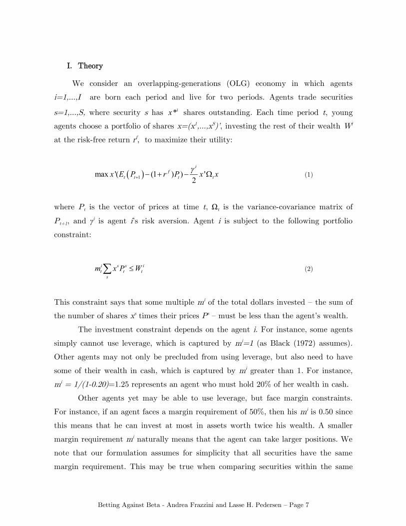
I. Theory
We consider an overlapping-generations (OLG) economy in which agents
i=1,...,I are born each period and live for two periods. Agents trade securities
s=1,...,S, where security s has *ix shares outstanding. Each time period t, young
agents choose a portfolio of shares x=(x1,...,xS)’, investing the rest of their wealth Wi
at the risk-free return rf, to maximize their utility:
1max '( (1 ) ) '2
if
t t t tx E P r P x x (1)
where Pt is the vector of prices at time t, Ωt is the variance-covariance matrix of
Pt+1, and γi is agent i’s risk aversion. Agent i is subject to the following portfolio
constraint:
i s s it t t
sm x P W (2)
This constraint says that some multiple mi of the total dollars invested – the sum of
the number of shares xs times their prices Ps – must be less than the agent’s wealth.
The investment constraint depends on the agent i. For instance, some agents
simply cannot use leverage, which is captured by mi=1 (as Black (1972) assumes).
Other agents may not only be precluded from using leverage, but also need to have
some of their wealth in cash, which is captured by mi greater than 1. For instance,
mi = 1/(1-0.20)=1.25 represents an agent who must hold 20% of her wealth in cash.
Other agents yet may be able to use leverage, but face margin constraints.
For instance, if an agent faces a margin requirement of 50%, then his mi is 0.50 since
this means that he can invest at most in assets worth twice his wealth. A smaller
margin requirement mi naturally means that the agent can take larger positions. We
note that our formulation assumes for simplicity that all securities have the same
margin requirement. This may be true when comparing securities within the same
Betting Against Beta - Andrea Frazzini and Lasse H. Pedersen – Page 8
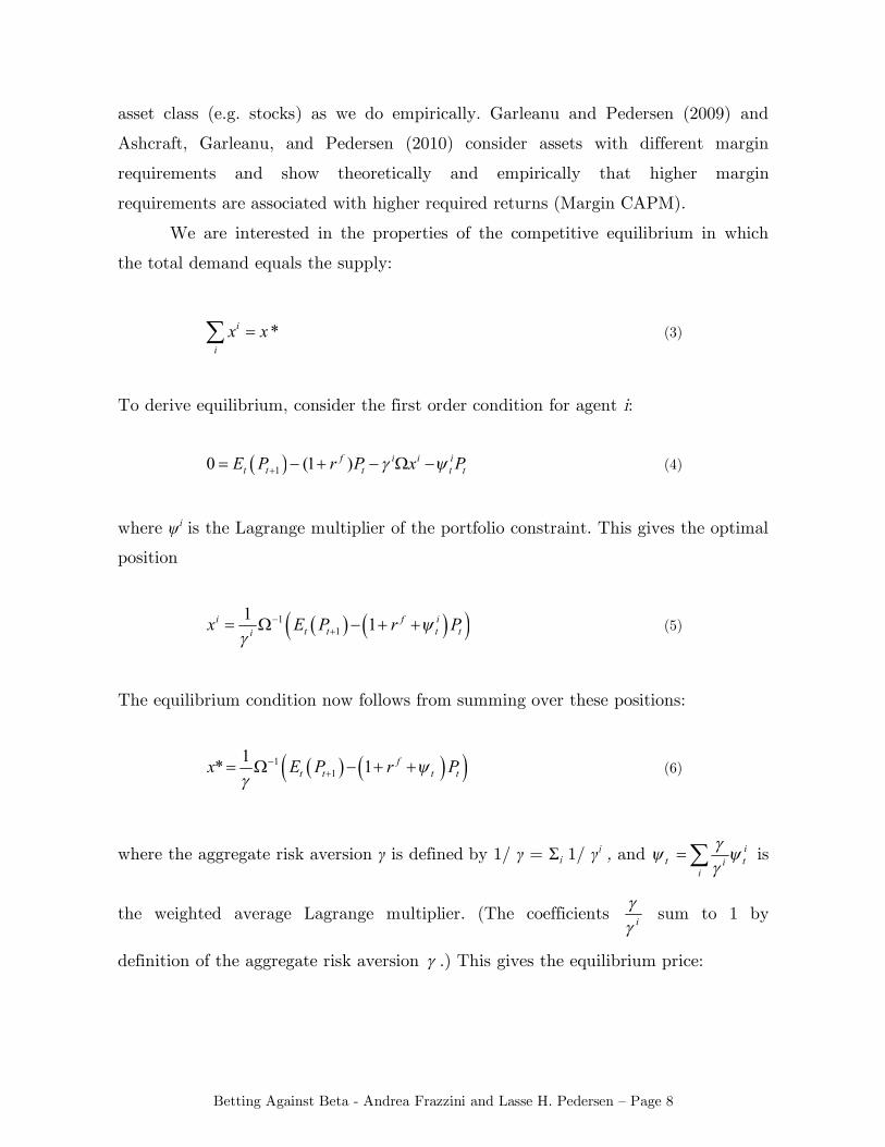
asset class (e.g. stocks) as we do empirically. Garleanu and Pedersen (2009) and
Ashcraft, Garleanu, and Pedersen (2010) consider assets with different margin
requirements and show theoretically and empirically that higher margin
requirements are associated with higher required returns (Margin CAPM).
We are interested in the properties of the competitive equilibrium in which
the total demand equals the supply:
*i
ix x (3)
To derive equilibrium, consider the first order condition for agent i:
10 (1 )f i i it t t t tE P r P x P (4)
where ψi is the Lagrange multiplier of the portfolio constraint. This gives the optimal
position
11
1 1i f it t t tix E P r P
(5)
The equilibrium condition now follows from summing over these positions:
11
1* 1 ft t t tx E P r P
(6)
where the aggregate risk aversion γ is defined by 1/ γ = Σi 1/ γi , and it ti
i
is
the weighted average Lagrange multiplier. (The coefficients i
sum to 1 by
definition of the aggregate risk aversion .) This gives the equilibrium price:
Betting Against Beta - Andrea Frazzini and Lasse H. Pedersen – Page 9
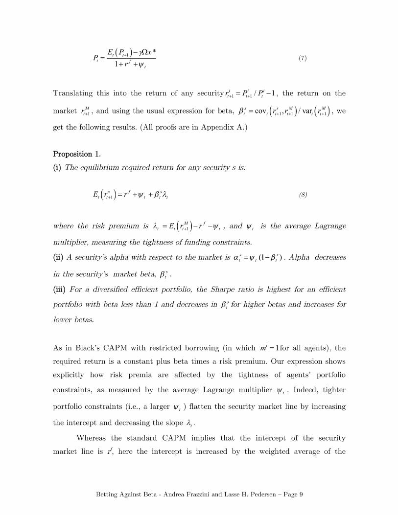
1 *1
t tt f
t
E P xP
r
(7)
Translating this into the return of any security 1 1 / 1i i it t tr P P , the return on the
market 1M
tr , and using the usual expression for beta, 1 1 1cov , / vars s M Mt t t t t tr r r , we
get the following results. (All proofs are in Appendix A.)
Proposition 1.
(i) The equilibrium required return for any security s is:
1s f s
t t t t tE r r (8)
where the risk premium is 1M f
t t t tE r r , and t is the average Lagrange
multiplier, measuring the tightness of funding constraints.
(ii) A security’s alpha with respect to the market is (1 )s st t t . Alpha decreases
in the security’s market beta, st .
(iii) For a diversified efficient portfolio, the Sharpe ratio is highest for an efficient
portfolio with beta less than 1 and decreases in st for higher betas and increases for
lower betas.
As in Black’s CAPM with restricted borrowing (in which 1im for all agents), the
required return is a constant plus beta times a risk premium. Our expression shows
explicitly how risk premia are affected by the tightness of agents’ portfolio
constraints, as measured by the average Lagrange multiplier t . Indeed, tighter
portfolio constraints (i.e., a larger t ) flatten the security market line by increasing
the intercept and decreasing the slope t .
Whereas the standard CAPM implies that the intercept of the security
market line is rf, here the intercept is increased by the weighted average of the
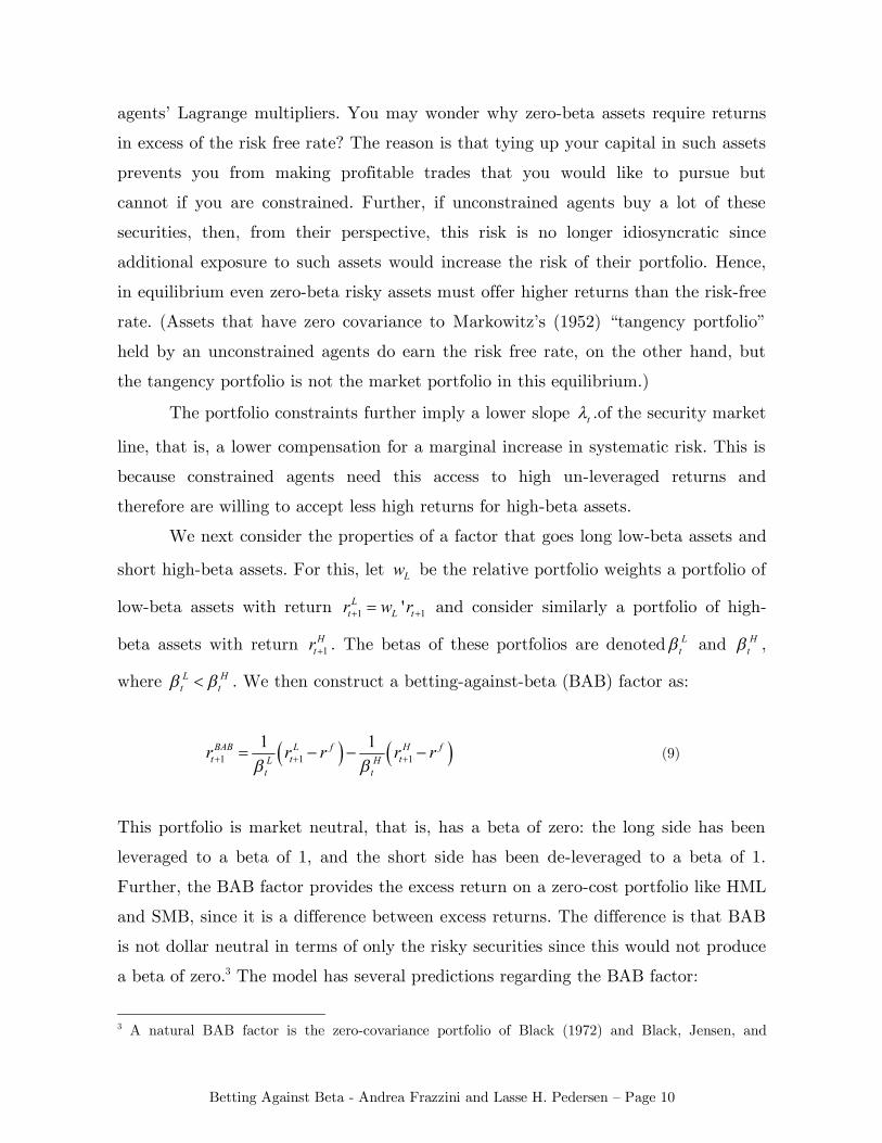
Betting Against Beta - Andrea Frazzini and Lasse H. Pedersen – Page 10
agents’ Lagrange multipliers. You may wonder why zero-beta assets require returns
in excess of the risk free rate? The reason is that tying up your capital in such assets
prevents you from making profitable trades that you would like to pursue but
cannot if you are constrained. Further, if unconstrained agents buy a lot of these
securities, then, from their perspective, this risk is no longer idiosyncratic since
additional exposure to such assets would increase the risk of their portfolio. Hence,
in equilibrium even zero-beta risky assets must offer higher returns than the risk-free
rate. (Assets that have zero covariance to Markowitz’s (1952) “tangency portfolio”
held by an unconstrained agents do earn the risk free rate, on the other hand, but
the tangency portfolio is not the market portfolio in this equilibrium.)
The portfolio constraints further imply a lower slope t .of the security market
line, that is, a lower compensation for a marginal increase in systematic risk. This is
because constrained agents need this access to high un-leveraged returns and
therefore are willing to accept less high returns for high-beta assets.
We next consider the properties of a factor that goes long low-beta assets and
short high-beta assets. For this, let Lw be the relative portfolio weights a portfolio of
low-beta assets with return 1 1'Lt L tr w r and consider similarly a portfolio of high-
beta assets with return 1H
tr . The betas of these portfolios are denoted Lt and H
t ,
where L Ht t . We then construct a betting-against-beta (BAB) factor as:
1 1 11 1BAB L f H f
t t tL Ht t
r r r r r (9)
This portfolio is market neutral, that is, has a beta of zero: the long side has been
leveraged to a beta of 1, and the short side has been de-leveraged to a beta of 1.
Further, the BAB factor provides the excess return on a zero-cost portfolio like HML
and SMB, since it is a difference between excess returns. The difference is that BAB
is not dollar neutral in terms of only the risky securities since this would not produce
a beta of zero.3 The model has several predictions regarding the BAB factor:
3 A natural BAB factor is the zero-covariance portfolio of Black (1972) and Black, Jensen, and
Betting Against Beta - Andrea Frazzini and Lasse H. Pedersen – Page 11
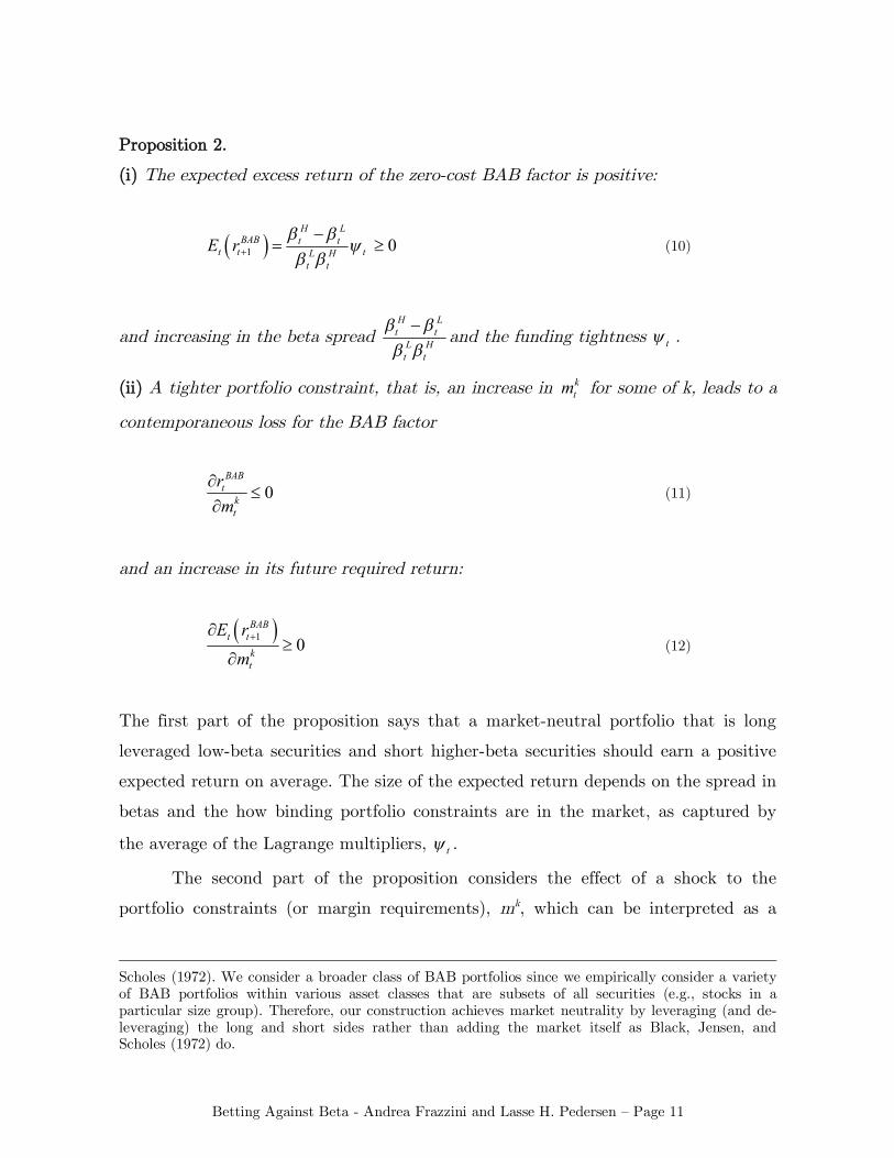
Proposition 2.
(i) The expected excess return of the zero-cost BAB factor is positive:
1 0H L
BAB t tt t tL H
t t
E r
(10)
and increasing in the beta spread H L
t tL Ht t
and the funding tightness t .
(ii) A tighter portfolio constraint, that is, an increase in ktm for some of k, leads to a
contemporaneous loss for the BAB factor
0BAB
tkt
rm
(11)
and an increase in its future required return:
1 0BAB
t tkt
E rm
(12)
The first part of the proposition says that a market-neutral portfolio that is long
leveraged low-beta securities and short higher-beta securities should earn a positive
expected return on average. The size of the expected return depends on the spread in
betas and the how binding portfolio constraints are in the market, as captured by
the average of the Lagrange multipliers, t .
The second part of the proposition considers the effect of a shock to the
portfolio constraints (or margin requirements), mk, which can be interpreted as a
Scholes (1972). We consider a broader class of BAB portfolios since we empirically consider a variety of BAB portfolios within various asset classes that are subsets of all securities (e.g., stocks in a particular size group). Therefore, our construction achieves market neutrality by leveraging (and de-leveraging) the long and short sides rather than adding the market itself as Black, Jensen, and Scholes (1972) do.
Betting Against Beta - Andrea Frazzini and Lasse H. Pedersen – Page 12
worsening of funding liquidity, a liquidity crisis in the extreme. Such a funding
liquidity shock results in losses for the BAB factor as its required return increases.
This happens as agents may need to de-lever their bets against beta or stretch even
further to buy the high-beta assets. This shows that the BAB factor is exposed to
funding liquidity risk – it loses when portfolio constraints become more binding.
Further, the market return tends to be low during such liquidity crises.
Indeed, a higher mk increases the required return of the market and reduces the
contemporaneous market return. Hence, while the BAB factor is market neutral on
average, liquidity shocks can lead to correlation between BAB and the market.
Another way of saying this is that low-beta securities fare poorly during times of
increased illiquidity relative to their betas, while high-beta securities fare less poorly
than their betas would suggest (“beta compression”):4
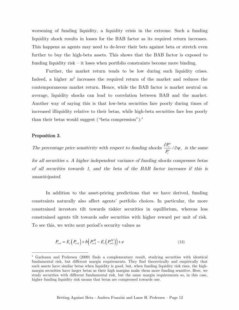
Proposition 3.
The percentage price sensitivity with respect to funding shocks /s
tts
t
PP
is the same
for all securities s. A higher independent variance of funding shocks compresses betas
of all securities towards 1, and the beta of the BAB factor increases if this is
unanticipated.
In addition to the asset-pricing predictions that we have derived, funding
constraints naturally also affect agents’ portfolio choices. In particular, the more
constrained investors tilt towards riskier securities in equilibrium, whereas less
constrained agents tilt towards safer securities with higher reward per unit of risk.
To see this, we write next period’s security values as
1 1 1 1M M
t t t t t tP E P b P E P e (13)
4 Garleanu and Pedersen (2009) finds a complementary result, studying securities with identical fundamental risk, but different margin requirements. They find theoretically and empirically that such assets have similar betas when liquidity is good, but, when funding liquidity risk rises, the high-margin securities have larger betas as their high margins make them more funding sensitive. Here, we study securities with different fundamental risk, but the same margin requirements so, in this case, higher funding liquidity risk means that betas are compressed towards one.
Betting Against Beta - Andrea Frazzini and Lasse H. Pedersen – Page 13
where b is a vector of market exposures and e is a vector of noise that is
uncorrelated with the market. With this, we have the following natural result for the
agents’ positions:
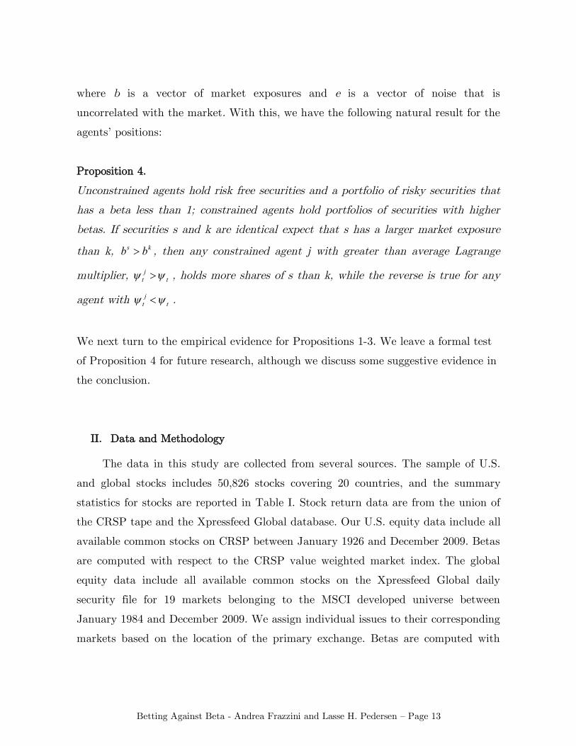
Proposition 4.
Unconstrained agents hold risk free securities and a portfolio of risky securities that
has a beta less than 1; constrained agents hold portfolios of securities with higher
betas. If securities s and k are identical expect that s has a larger market exposure
than k, s kb b , then any constrained agent j with greater than average Lagrange
multiplier, jt t , holds more shares of s than k, while the reverse is true for any
agent with jt t .
We next turn to the empirical evidence for Propositions 1-3. We leave a formal test
of Proposition 4 for future research, although we discuss some suggestive evidence in
the conclusion.
II. Data and Methodology
The data in this study are collected from several sources. The sample of U.S.
and global stocks includes 50,826 stocks covering 20 countries, and the summary
statistics for stocks are reported in Table I. Stock return data are from the union of
the CRSP tape and the Xpressfeed Global database. Our U.S. equity data include all
available common stocks on CRSP between January 1926 and December 2009. Betas
are computed with respect to the CRSP value weighted market index. The global
equity data include all available common stocks on the Xpressfeed Global daily
security file for 19 markets belonging to the MSCI developed universe between
January 1984 and December 2009. We assign individual issues to their corresponding
markets based on the location of the primary exchange. Betas are computed with
Betting Against Beta - Andrea Frazzini and Lasse H. Pedersen – Page 14
respect to the corresponding MSCI local market index5. All returns are in USD and
excess returns are above the US Treasury bill rate. We consider alphas with respect
to the market and US factor returns based on size (SMB), book-to-market (HML),
momentum (UMD), and liquidity risk.6
We also consider a variety of other assets and Table II contains the list
instruments and the corresponding data availability ranges. We obtain U.S.
Treasury bond data from the CRSP US Treasury Database. Our analysis focuses on
monthly returns (in excess of the 1-month Treasury bill) on the Fama Bond
portfolios for maturities ranging from 1 to 10 years between January 1952 and
December 2009. Returns are an equal-weighted average of the unadjusted holding
period return for each bond in the portfolios. Only non-callable, non-flower notes and
bonds are included in the portfolios. Betas are computed with respect to an equally
weighted portfolio of all bonds in the database.
We collect aggregate corporate bond index returns from Barclays Capital’s
Bond.Hub database.7 Our analysis focused on monthly returns (in excess of the 1-
month Treasury bill) on 4 aggregate US credit indices with maturity ranging from
one to ten years and nine investment grade and high yield corporate bond portfolios
with credit risk ranging from AAA to Ca-D and “Distressed”8. The data cover the
period between January 1973 and December 2009 although the data availability
varies depending on the individual bond series. Betas are computed with respect to
an equally weighted portfolio of all bonds in the database.
We also study futures and forwards on country equity indexes, country bond
indexes, foreign exchange, and commodities. Return data are drawn from the
internal pricing data maintained by AQR Capital Management LLC. The data is
collected from a variety of sources and contains daily returns on futures, forwards or
swaps contracts in excess of the relevant financing rate. The type of contract for
each asset depends on availability or the relative liquidity of different instruments.
Prior to expiration positions are rolled over into next most liquid contract. The
5 Our results are robust to the choice of benchmark (local vs. global). We report these tests in the Appendix. 6 SMB, HML, UMD are from Ken French’s website and the liquidity risk factor is from WRDS. 7 The data can be downloaded at https://live.barcap.com 8 The distress index was provided to us by Credit Suisse.
Betting Against Beta - Andrea Frazzini and Lasse H. Pedersen – Page 15
rolling date’s convention differs across contracts and depends on the relative
liquidity of different maturities. The data cover the period between 1963 and 2009,
although the data availability varies depending on the asset class. For more details
on the computation of returns and data sources see Moskowitz, Ooi, and Pedersen
(2010), Appendix A. For equity indexes, country bonds and currencies, betas are
computed with respect to a GDP-weighted portfolio, and, for commodities, betas are
computed with respect to a diversified portfolio that gives equal risk weight across
commodities.
Finally, we use the TED spread as a proxy for time periods where credit
constraint are more likely to be binding (as Garleanu and Pedersen (2009) and
others). The TED spread is defined as the difference between the three-month
EuroDollar LIBOR rate on the three-month U.S. Treasuries rate. Our TED data run
from December 1984 to December 2009.
Estimating Betas
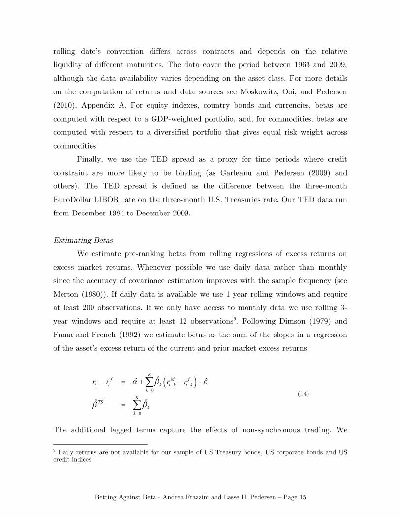
We estimate pre-ranking betas from rolling regressions of excess returns on
excess market returns. Whenever possible we use daily data rather than monthly
since the accuracy of covariance estimation improves with the sample frequency (see
Merton (1980)). If daily data is available we use 1-year rolling windows and require
at least 200 observations. If we only have access to monthly data we use rolling 3-
year windows and require at least 12 observations9. Following Dimson (1979) and
Fama and French (1992) we estimate betas as the sum of the slopes in a regression
of the asset’s excess return of the current and prior market excess returns:
0
0
ˆˆ ˆ
ˆ ˆ
Kf M f
t t k t k t kk
KTS
kk
r r r r
(14)
The additional lagged terms capture the effects of non-synchronous trading. We
9 Daily returns are not available for our sample of US Treasury bonds, US corporate bonds and US credit indices.
Betting Against Beta - Andrea Frazzini and Lasse H. Pedersen – Page 16
include lags up to K = 5 trading days. When the sample frequency is monthly, we
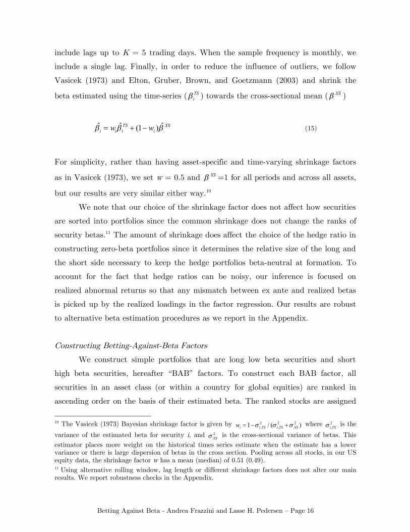
include a single lag. Finally, in order to reduce the influence of outliers, we follow
Vasicek (1973) and Elton, Gruber, Brown, and Goetzmann (2003) and shrink the
beta estimated using the time-series ( TSi ) towards the cross-sectional mean ( XS )
ˆ ˆ ˆ(1 )TS XSi i i iw w (15)
For simplicity, rather than having asset-specific and time-varying shrinkage factors
as in Vasicek (1973), we set w = 0.5 and XS =1 for all periods and across all assets,
but our results are very similar either way.10
We note that our choice of the shrinkage factor does not affect how securities
are sorted into portfolios since the common shrinkage does not change the ranks of
security betas.11 The amount of shrinkage does affect the choice of the hedge ratio in
constructing zero-beta portfolios since it determines the relative size of the long and
the short side necessary to keep the hedge portfolios beta-neutral at formation. To
account for the fact that hedge ratios can be noisy, our inference is focused on
realized abnormal returns so that any mismatch between ex ante and realized betas
is picked up by the realized loadings in the factor regression. Our results are robust
to alternative beta estimation procedures as we report in the Appendix.
Constructing Betting-Against-Beta Factors
We construct simple portfolios that are long low beta securities and short
high beta securities, hereafter “BAB” factors. To construct each BAB factor, all
securities in an asset class (or within a country for global equities) are ranked in
ascending order on the basis of their estimated beta. The ranked stocks are assigned
10 The Vasicek (1973) Bayesian shrinkage factor is given by 2 2 2
, ,1 / ( )i i TS i TS XSw where 2,i TS is the
variance of the estimated beta for security i, and 2XS is the cross-sectional variance of betas. This
estimator places more weight on the historical times series estimate when the estimate has a lower variance or there is large dispersion of betas in the cross section. Pooling across all stocks, in our US equity data, the shrinkage factor w has a mean (median) of 0.51 (0.49). 11 Using alternative rolling window, lag length or different shrinkage factors does not alter our main results. We report robustness checks in the Appendix.
Betting Against Beta - Andrea Frazzini and Lasse H. Pedersen – Page 17
to one of two portfolios: low beta and high beta. Securities are weighted by the
ranked betas and the portfolios are rebalanced every calendar month. Both portfolios
are rescaled to have a beta of one at portfolio formation. The BAB is the zero-cost
zero-beta portfolio (9) that is long the low-beta portfolio and shorts the high-beta
portfolio. For example, on average the U.S. stock BAB factor is long $1.5 worth of
low-beta stocks (financed by shorting $1.5 of risk free securities) and short $0.7
worth of high-beta stocks (with $0.7 earning the risk-free rate).
III. Betting Against Beta in Each Asset Class
Cross section of stock returns
We now test how the required premium varies in the cross-section of beta-
sorted securities (Proposition 1) and the hypothesis that long/short BAB factors
have positive average returns (Proposition 2). Table III reports our tests for U.S.
stocks. We consider 10 beta-sorted portfolios and report their average returns,
alphas, market betas, volatilities, and Sharpe ratios. The average returns of the
different beta portfolios are similar, which is the well-known flat security market
line. Hence, consistent with Proposition 1 and with Black (1972), alphas decline
almost monotonically from low-beta to high-beta portfolios. Indeed, alphas decline
both when estimated relative to a 1-, 3-, 4-, and 5-factor model. Also, Sharpe ratios
decline monotonically from low-beta to high-beta portfolios. As we discuss in detail
below, declining alphas and Sharpe ratios across beta sorted portfolios is a general
phenomenon across asset classes. As a overview of these results, the Sharpe ratios of
all the beta-sorted portfolios considered in this paper are plotted in Figure B1 in the
Appendix.
The rightmost column of Table III reports returns of the betting-against-beta
(BAB) factor of Equation (9), that is, a portfolio that is long a levered basket of
low-beta stocks and short a de-levered basket of high-beta stocks such as to keep the
portfolio beta-neutral. Consistent with Proposition 2, the BAB factor delivers a high
average return and a high alpha. Specifically, the BAB factor has Fama and French
(1993) abnormal returns of 0.69% per month (t-statistic = 6.55). Additionally
Betting Against Beta - Andrea Frazzini and Lasse H. Pedersen – Page 18
adjusting returns for Carhart’s (1997) momentum-factor, the BAB portfolio earns
abnormal returns of 0.55% per month (t-statistic = 5.12). Last, we adjust returns
using a 5-factor model by adding the traded liquidity factor by Pastor and
Stambaugh (2003), yielding an abnormal BAB return of 0.46% per month (t-statistic
= 2.93) 12. We note that while the alpha of the long-short portfolio is consistent
across regressions, the choice of risk adjustment influences the relative alpha
contribution of the long and short sides of the portfolio. Figure B2 in the Appendix
plots the annual abnormal returns of the BAB stock portfolio.
We next consider beta-sorted portfolios for global stocks. We use all 19 MSCI
developed countries except the U.S. (to keep the results separate from the U.S.
results above), and we do this in two ways: We consider global portfolios where all
global stocks are pooled together (Table IV), and we consider results separately for
each country (Table V). The global portfolio is country neutral that is stocks are
assignee to low (high) beta basket within each country.13
The results for our pooled sample of global equities in Table IV mimic the
U.S. results: Alphas and Sharpe ratios of the beta-sorted portfolios decline (although
not perfectly monotonically) with betas, and the BAB factor earns risk-adjusted
returns between 0.42% and 0.71% per month depending on the choice of risk
adjustment with t-statistics ranging from 2.22 to 3.72.
Table V shows the performance of the BAB factor within each individual
country. The BAB delivers positive Sharpe ratios in 18 of the 19 MSCI developed
countries and positive 4-factor alphas in 16 out of 19, displaying a strikingly
consistent pattern across equity markets. The BAB returns are statistically
significantly positive in 9 countries. Of course, the small number of stocks in our
sample in many of the countries (with some countries having only a few dozen
securities traded) makes it difficult to reject the null hypothesis of zero return in
each individual factor. Figure B3 in the Appendix plots the annual abnormal returns
of the BAB global portfolio.
12 Note that Pastor and Stambaugh (2003) liquidity factor is available on WRDS only between 1968 and 2008 thus cutting about 50% of our observations. 13 We keep the global portfolio country neutral since we report results for equity indices BAB separately in table IX.
Betting Against Beta - Andrea Frazzini and Lasse H. Pedersen – Page 19
Tables B1 and B2 in the Appendix report factors loadings. On average, the
U.S. BAB factor invests $1.52 long ($1.58 for Global BAB) and $0.71 short ($0.84
for Global BAB). The larger long investment is meant to make the BAB factor
market neutral since the long stocks have smaller betas. The U.S. BAB factor
realizes a small positive market loading, indicating that our ex-ante beta are
measured with noise. The other factor loadings indicates that, relative to high-beta
stocks, low-beta stocks are likely to be smaller, have higher book-to-market ratios,
and have higher return over the prior 12 months, although none of the loadings can
explain the large and significant abnormal returns.
The Appendix reports further tests and additional robustness checks. We split
the sample by size and time periods. We control for idiosyncratic volatility (both
level and changes) and report results for alternative definition of betas. All the
results tell a consistent story: equity beta-neutral portfolios that bet against betas
earn significant risk-adjusted returns.
Treasury Bonds
Table VI reports results for US Treasury bonds. As before, we report average
excess returns of bond portfolios formed by sorting on beta in the previous month. In
the cross section of Treasury bonds, ranking on betas with respect to an aggregate
Treasury bond index is empirically equivalent to ranking on duration or maturity.
Therefore, in Table VI one can think of the term “beta,” “duration,” or “maturity”
in an interchangeable fashion. The rightmost column reports returns of the BAB
factor. Abnormal returns are computed with respect to a one-factor model: alpha is
the intercept in a regression of monthly excess return on an equally weighted
Treasury bond excess market return.
The results show that the phenomenon of a flat security market line is not
limited to the cross section of stock returns. Indeed, consistent with Proposition 1,
alphas decline monotonically with beta. Likewise, Sharpe ratios decline
monotonically from 0.73 for low-beta (short maturity) bonds to 0.27 for high-beta
(long maturity) bonds. Further, the bond BAB portfolio delivers abnormal returns of
Betting Against Beta - Andrea Frazzini and Lasse H. Pedersen – Page 20
0.16% per month (t-statistic = 6.37) with a large annual Sharpe ratio of 0.85. Figure
B4 in the Appendix plots the annual time series of returns.
Since the idea that funding constraints have a significant effect on the term
structure of interest may be surprising, let us illustrate the economic mechanism
that may be at work. Suppose an agent, e.g., a pension fund, has $1 to allocate to
Treasuries with a target excess return on 1.65% per year. One way to achieve this
return target is to invest $1 in a portfolio of 10-year bonds as seen in Table VI. If
instead the agent invests in 1-year Treasuries then he would need to invest $4.76 if
all maturities had the same Sharpe ratio. This is because 10-year Treasures are 4.76
times more volatile than 1-year Treasuries. Hence, the agent would need to borrow
an additional $3.76 to lever his investment in 1-year bonds. If the agent has leverage
limits (or prefers lower leverage), then he would strictly prefer the 10-year Treasuries
in this case.
According to our theory, the 1-year Treasuries therefore must offer higher
returns and higher Sharpe ratios, flattening the security market line for bonds. This
is the case empirically. Empirically, the return target can be achieved with by
investing $2.7 in 1-year bonds. While a constrained investor may still prefer an un-
leveraged investment in 10-year bonds, unconstrained investors now prefer the
leveraged low-beta bonds, and the market can clear.
While the severity of leverage constraints varies across market participants, it
appears plausible that a 2.7 to 1 leverage (on this part of the portfolio) makes a
difference for some large investors such as pension funds.
Credit
We next test our model using several credit portfolios. In Table VII, the test
assets are monthly excess returns of corporate bond indexes with maturity ranging
from 1 to 10 years. Table VII panel A shows that the credit BAB portfolio delivers
abnormal returns of 0.13% per month (t-statistic = 4.91) with a large annual Sharpe
ratio of 0.88. Further, alphas and Sharpe ratios decline monotonically, with Sharpe
ratios ranging from 0.79 to 0.64 from low beta (short maturity) to high beta (long
maturity bonds).
Betting Against Beta - Andrea Frazzini and Lasse H. Pedersen – Page 21
Panel B of Table VII reports results for portfolio of US credit indices where
we try to isolate the credit component by hedging away the interest rate risk. Given
the results on Treasuries in Table VI we are interested in testing a pure credit
version of the BAB portfolio. Each calendar month we run 1-year rolling regressions
of excess bond returns on excess return on Barclay’s US government bond index. We
construct test assets by going long the corporate bond index and hedging this
position by shorting the appropriate amount of the government bond index:
1ˆ( ) ( )CDS f f USGOV f
t t t t t t tr r r r r r , where 1t̂ is the slope coefficient estimated in
an expanding regression using data up to month t-1. One interpretation of this
returns series is that it approximately mimics the returns on a Credit Default Swap
(CDS). We compute market returns by taking equally weighted average of these
hedged returns, and compute betas and BAB portfolios as before. Abnormal returns
are computed with respect to a two factor model: alpha is the intercept in a
regression of monthly excess return on the equally weighted average pseudo-CDS
excess return and the monthly return on the (un-hedged) BAB factor for US credit
indices in the rightmost column of Table VII panel B. The addition of the un-hedged
BAB factor on the right hand side is an extra check to test a pure credit version of
the BAB portfolio.
The results in Panel B of Table VII tell the same story as Panel A: the CDS
BAB portfolio delivers significant returns of 0.08% per month (t-statistics = 3.65)
and Sharpe ratios decline monotonically from low beta to high beta assets. Figure B5
in the Appendix plots the annual time series of returns.
Last, in Table VIII we report results where the test assets are credit indexes
sorted by rating, ranging from AAA to Ca-D and Distressed. Consistent with all our
previous results, we find large abnormal returns of the BAB portfolios (0.56% per
month with a t-statistics = 4.02), and declining alphas and Sharpe ratios across beta
sorted portfolios. Figure B6 in the Appendix plots the annual time series of returns.
Equity indexes, country bond indexes, foreign exchange and commodities
Table IX reports results for equity indexes, country bond indexes, foreign
exchange and commodities. The BAB portfolio delivers positive return in each of the
Betting Against Beta - Andrea Frazzini and Lasse H. Pedersen – Page 22
four asset classes, with annualized Sharpe ratio ranging from 0.22 to 0.51. The
magnitude of returns is large, but the BAB portfolios in these assets are much more
volatile and, as a result, we are only able to reject the null hypothesis of zero
average return for global equity indexes. We can, however, reject the null hypothesis
of zero returns for combination portfolios than include all or some combination of
the four asset classes, taking advantage of diversification. We construct a simple
equally weighted BAB portfolio. To account for different volatility across the four
asset classes, in month t we rescale each return series to 10% annualized volatility
using rolling 3-year estimate up to moth t-1 and then equally weight the return
series and their respective market benchmark. This corresponds to a simple
implementable portfolio that targets 10% BAB volatility in each asset classes. We
report results for an All futures combo including all four asset classes and a Country
Selection combo including only Equity indices, Country Bonds and Foreign
Exchange. The BAB All Futures and Country Selection deliver abnormal return of
0.52% and 0.71% per month (t-statistics = 4.50 and 4.42). Figure B7 in the
Appendix plots the annual time series of returns.
To summarize, the results in Table III—IX strongly support the predictions
that alphas decline with beta and BAB factors earn positive excess returns in each
asset class. Figure A1 illustrate the remarkably consistent pattern of declining
Sharpe ratios in each asset class. Clearly, the flat security market line, documented
by Black, Jensen, Scholes (1972) for U.S. stocks, is a pervasive phenomenon that we
find across markets and asset classes. Putting all the BAB factors together produces
a large and significant abnormal return of 0.77% per month (t-statistics of 8.8) as
seen in Table IX panel B.
This evidence is consistent with of a model in which some investors are
prohibited from using leverage and other investors’ leverage is limited by margin
requirements, generating positive average return of factors that are long a leveraged
portfolio of low-beta assets and short a portfolio of high-beta assets. To further
examine this explanation of what appears to be a pervasive phenomenon, we next
turn to tests the cross-sectional time-series predictions of the model.
Betting Against Beta - Andrea Frazzini and Lasse H. Pedersen – Page 23
IV. Beta Compression
In this section, we tests Proposition 3 that betas are compressed towards 1
during times with shocks to funding constraints. This model prediction generates
two testable hypotheses. The first is a direct prediction on the cross-sectional of
betas: the cross-sectional dispersion in betas should be lower when individual credit
constraints are more likely to be binding. The second is a prediction on the
conditional market betas of BAB portfolios: although beta neutral at portfolio
formation (and on average), a BAB factor should tend to realize positive market
exposure when individual credit constraints are more likely to be binding. We
present results for both predictions in Table X.
We use the TED spread as a proxy of funding liquidity conditions. Our tests
rely on the assumption that high levels of TED spread (or, similarly, high levels of
TED spread volatility) correspond to times when investors are more likely to face
shocks to their funding conditions. Since we expect that funding shocks affect the
overall market return, we confirm that the monthly correlation between the TED
spread (either level or 1-month changes) and the CRSP value weighted index is
negative, around -25%.
We test the model’s predictions about the dispersion in betas using our
samples of US and Global equities which have the largest cross sections of securities.
The sample runs from December 1984 (the first available date for the TED spread)
to 2009.
Table X, Panel A shows the cross-sectional dispersion in betas in different
time periods sorted by likelihood of binding credit constraints for U.S. stocks. Panel
B shows the same for global stocks. Each calendar month we compute cross-sectional
standard deviation, mean absolute deviation and inter-quintile range in betas for all
stocks in the universe. We assign the TED spread into three groups (low, medium,
and high) based on full sample breakpoints (top and bottom 1/3) and regress the
times series of the cross-sectional dispersion measure on the full set of dummies
(without intercept). Table X shows that, consistent with Proposition 3, the cross-
sectional dispersion in betas is lower when credit constraints are more likely to be
Betting Against Beta - Andrea Frazzini and Lasse H. Pedersen – Page 24
biding. The average cross-sectional standard deviation of US equity betas in periods
of low spreads is 0.47 while the dispersion shrinks to 0.35 in tight credit environment
and the difference is highly statistical significant (t-statistics = -10.72). The tests
based on the other dispersion measures and the global data all tell a consistent story:
the cross-sectional dispersion in beta shrink at times where credit is more likely to be
rationed.
Panel C and D reports conditional market betas of the BAB portfolios based
on the credit environment for, respectively, U.S. and global stocks. We run factor
regression and allow loadings on the market portfolio to vary as function of the
realized TED spread. The dependent variable is the monthly return of the BAB
portfolio. The explanatory variables are the monthly returns of the market portfolio,
Fama and French (1993) mimicking portfolios and Carhart (1997) momentum factor.
Market betas are allowed to vary across TED spread regimes (low, neutral and high)
using the full set of TED dummies. We are interested in testing the hypothesis that
ˆ ˆMKT MKThigh low where ˆ MKT
high ( ˆ MKTlow ) is the conditional market beta in times when credit
constraints are more (less) likely to be binding. Panel B reports loading on the
market factor corresponding to different time periods sorted by the credit
environment. We include the full set of explanatory variables in the regression but
only report the market loading. The results are consistent with Proposition 3:
although the BAB factor is both ex ante and ex post market neutral on average, the
conditional market loading on the BAB factor is function of the credit environment.
Indeed, recall from Table III that the realized average market loading is an
insignificant 0.03, while Table X shows that when credit is more likely to be
rationed, the BAB-factor beta rises to 0.30. The rightmost column shows that
variation in realized between tight and relaxed credit environment is large (0.51),
and we are safely able to reject the null that ˆ ˆMKT MKThigh low (t-statistics 3.64).
Controlling for 3 or 4 factors does not alter the results, although loadings on the
other factors absorb some the difference. The results for our sample of global equities
are similar as shown and panel D.
To summarize, the results in Table X support the prediction of our model
that there is beta compression in times of funding liquidity risk. This can be
Betting Against Beta - Andrea Frazzini and Lasse H. Pedersen – Page 25
understood in two ways. First, more discount-rate volatility that affects all securities
the same way compresses beta. A deeper explanation is that, as funding conditions
get worse, all prices tend to go down, but high-beta assets do not drop as much as
their ex-ante beta suggests because the securities market line flattens at such times,
providing support for high-beta assets. Conversely, the flattening of the security
market line makes low-beta assets drop more than their ex-ante betas suggest.
V. Time Series Tests
In this section, we test Proposition 2’s predictions for the time-series of the
BAB returns. When funding constraints become more binding (e.g., because margin
requirements rise), the required BAB premium increases and the realized BAB
returns becomes negative.
We take this prediction to the data using the TED spread as a proxy of
funding conditions as in Section IV. Figure 2 shows the realized return on the U.S.
BAB factor and the (negated) TED spread. We plot 3-years rolling average of both
variables. The figure shows that the BAB returns tend to be lower in periods of high
TED spread, consistent with Proposition 2.
We next test the hypothesis in a regression framework for each of the BAB
factors across asset classes, as reported in Table XI. The first column simply
regresses the U.S. BAB factor on the contemporaneous level of the TED spread.
Consistent with Proposition 2, we find a negative and significant relation, confirming
the relation that is visually clear in Figure 2. Column (2) has a similar result when
controlling for a number of control variables.
The control variables are the market returns, the 1-month lagged BAB
return, the ex ante Beta Spread, and the Short Volatility Returns. The Beta Spread
is equal to ( ) /S L S L and measures the beta difference between the long and
short side of the BAB portfolios. The Short Volatility Returns is the return on a
portfolio that is short closest-to-the-money, next-to-expire straddles on the S&P500
index, and measures short to aggregate volatility.
Betting Against Beta - Andrea Frazzini and Lasse H. Pedersen – Page 26
In columns (3) and (4), we decompose the TED spread into its level and
change: The Change in TED Spread is equal to TED in month t minus the median
spread over the past 3 years while Lagged TED Spread is the median spread over
the past 3 years. We see that both the lagged level and contemporaneous change in
the TED spread are negatively related to the BAB returns. If the TED spread
measures that agents’ funding constraint (given by in the model) are tight, then
the model predicts a negative coefficient for the change in TED and a positive
coefficient for the lagged level. Hence, the coefficient for the lagged level is not
consistent with the model under this interpretation of the TED spread. If, instead, a
high TED spread indicates that agents’ funding constraints are worsening, then the
results could be consistent with the model. Under this interpretation, a high TED
spread could indicate that banks are credit constrained and that banks over time
tighten other investors’ credit constraints, thus leading to a deterioration of BAB
returns over time, if this is not fully priced in.
Columns (5)-(8) of Table XI reports panel regressions for global stock BAB
factors, and columns (9)-(12) for all the BAB factors. These regressions include fixed
effect and standard errors are clustered by date. We consistently find a negative
relationship between BAB returns and the TED spread.
In addition to the TED spread, the ex ante Beta Spread, ( ) /S L S L , is of
interest since Proposition 2 predicts that the ex ante beta spread should predict
BAB returns positively. Consistent with the model, Table XI shows that the
estimated coefficient for the Beta Spread is positive in all six regressions where it is
included, and statistically significant in three regressions that control for the lagged
TED spread.
To ensure that these panel-regression estimates are not driven by a few asset
classes, we also run a separate regression for each BAB factor on the TED spread.
Figure 3 plots the t-statistics of the slope estimate on the TED spread. Although we
are not always able to reject the null of no effect for each individual factor, the
slopes estimates display a consistent pattern: we find negative coefficients in 16 out
of the 19 asset classes, with Credit and Treasuries being the exceptions. Obviously
the exceptions could be just noise, but positive returns to BAB portfolios during
Betting Against Beta - Andrea Frazzini and Lasse H. Pedersen – Page 27
liquidity crises (i.e., high TED periods) could possibly be related to “flight to
quality” in which some investors switch towards assets that are closer to money-
market instruments, or related to central banks cutting short-term yields to
counteract liquidity crises. Table A7 in the Appendix provides more details on the
BAB returns in different environments.
VI. Conclusion
All real-world investors face funding constraints such as leverage constraints
and margin requirements, and these constraints influence investors’ required returns
across securities and over time. Consistent with the idea that investors prefer un-
leveraged risky assets to leveraged safe assets, which goes back to Black (1972), we
find empirically that portfolios of high-beta assets have lower alphas and Sharpe
ratios than low-beta assets. The security market line is not only flat for U.S. equities
(as reported by Black, Jensen, and Scholes (1972)), but we also find this flatness for
18 of 19 global equity markets, in Treasury markets, for corporate bonds sorted by
maturity and by rating, and in futures markets. We show how this deviation from
the standard CAPM can be captured using betting-against-beta factors, which may
also be useful as control variables in future research. The return of the BAB factor
rivals that of standard asset pricing factors such as value, momentum, and size in
terms of economic magnitude, statistical significance, and robustness across time
periods, sub-samples of stocks, and global asset classes.
Extending the Black (1972) model, we consider the implications of funding
constraints for cross-sectional and time-series asset returns: We show that increased
funding liquidity risk compresses betas in the cross section of securities towards 1,
leading to an increased beta for the BAB factor, and we find consistent evidence
empirically. In the time series, we show that increased funding illiquidity should lead
to losses for the BAB factor, and we find consistent evidence in all the asset classes
that we study except Treasuries and credit.
Our model also has implications for agents’ portfolio selection (Proposition 4).
While we leave rigorous tests of these predictions for future research, we conclude
Betting Against Beta - Andrea Frazzini and Lasse H. Pedersen – Page 28
with some suggestive ideas consistent with the model’s predictions. Our model
predicts that agents with access to leverage buy low-beta securities and lever them
up. One such group of agents is private equity (PE) funds involved in leveraged
buyouts (LBOs). Our model predicts that the stocks bought by PE firms have a
lower beta than 1 before they buy them. Further, when the private equity firm sells
the firm back to the public, the model predicts that the beta has increased. Also,
banks have relatively easy access to leverage (e.g., through their depositors) so the
model predicts that banks own leveraged positions in securities with low-beta.
Indeed, anecdotal evidence suggests that banks hold leveraged portfolios of high-
rated bonds, e.g. mortgage bonds. Further, shadow banks such as special investment
vehicles (SIVs) had in some cases infinitely leveraged portfolios of short-dated high-
rated fixed-income securities. Conversely, the model predicts that investors that are
particularly restricted by constraints buy high-beta assets. For instance, mutual
funds may be biased to holding high-beta stocks because of their limited leveraged
(Karceski (2002)).
Betting Against Beta - Andrea Frazzini and Lasse H. Pedersen – Page 29
References
Acharya, V. V., and L. H. Pedersen (2005), “Asset Pricing with Liquidity Risk,"
Journal of Financial Economics, 77, 375-410.
Ang, A., R. Hodrick, Y. Xing, X. Zhang (2006), “The Cross-Section of Volatility and
Expected Returns,” Journal of Finance, 61, pp. 259-299.
– (2009), “High Idiosyncratic Volatility and Low Returns: International and Further
U.S. Evidence,” Journal of Financial Economics, 91, pp. 1-23.
Ashcraft, A., N. Garleanu, and L.H. Pedersen (2010), “Two Monetary Tools:
Interest Rates and Haircuts,” NBER Macroeconomics Annual, forthcoming.
Baker, M., B. Bradley, and J. Wurgler (2010), “Benchmarks as Limits to Arbitrage:
Understanding the Low Volatility Anomaly,” working paper, Harvard.
Black, F. (1972), “Capital market equilibrium with restricted borrowing,” Journal of
business, 45, 3, pp. 444-455.
– (1992), “Beta and Return,” The Journal of Portfolio Management, 20, pp. 8-18.
Black, F., M.C. Jensen, and M. Scholes (1972), “The Capital Asset Pricing Model:
Some Empirical Tests.” In Michael C. Jensen (ed.), Studies in the Theory of Capital
Markets, New York, pp. 79-121.
Brennan, M.J., (1971), “Capital market equilibrium with divergent borrowing and
lending rates.” Journal of Financial and Quantitative Analysis 6, 1197-1205.
Brennan, M.J. (1993), “Agency and Asset Pricing.” University of California, Los
Angeles, working paper.
Betting Against Beta - Andrea Frazzini and Lasse H. Pedersen – Page 30
Brunnermeier, M. and L.H. Pedersen (2009), “Market Liquidity and Funding
Liquidity,” The Review of Financial Studies, 22, 2201-2238.
Carhart, M. (1997), "On persistence in mutual fund performance", Journal of
Finance 52, 57–82.
Cuoco, D. (1997), “Optimal consumption and equilibrium prices with portfolio
constraints and stochastic income," Journal of Economic Theory, 72(1), 33-73.
Dimson, E. (1979), “Risk Measurement when Shares are Subject to Infrequent
Trading,” Journal of Financial Economics, 7, 197–226.
Duffee, G. (2010), “Sharpe Ratios in Term Structure Models,” Johns Hopkins
University, working paper.
Elton, E.G., M.J. Gruber, S. J. Brown and W. Goetzmannn: "Modern Portfolio
Theory and Investment", Wiley: New jersey.
Fama, E.F. (1984), “The Information in the Term Structure,” Journal of Financial
Economics, 13, 509-528.
Fama, E.F. (1986), “Term Premiums and Default Premiums in Money Markets,”
Journal of Financial Economics, 17, 175-196.
Fama, E.F. and French, K.R. (1992), “The cross-section of expected stock returns,”
Journal of Finance, 47, 2, pp. 427-465.
Fama, E.F. and French, K.R. (1993), "Common risk factors in the returns on stocks
and bonds", Journal of Financial Economics 33, 3–56.
Betting Against Beta - Andrea Frazzini and Lasse H. Pedersen – Page 31
Fu, F. (2009), “Idiosyncratic risk and the cross-section of expected stock returns,”
Journal of Financial Economics, vol. 91:1, 24-37.
Garleanu, N., and L. H. Pedersen (2009), “Margin-Based Asset Pricing and
Deviations from the Law of One Price," UC Berkeley and NYU, working paper.
Gibbons, M. (1982), “Multivariate tests of financial models: A new approach,”
Journal of Financial Economics, 10, 3-27.
Gromb, D. and D. Vayanos (2002), “Equilibrium and Welfare in Markets with
Financially Constrained Arbitrageurs,” Journal of Financial Economics, 66, 361–407.
Hindy, A. (1995), “Viable Prices in Financial Markets with Solvency Constraints,"
Journal of Mathematical Economics, 24(2), 105-135.
Kandel, S. (1984), “The likelihood ratio test statistic of mean-variance efficiency
without a riskless asset,” Journal of Financial Economics, 13, pp. 575-592.
Karceski, J. (2002), “Returns-Chasing Behavior, Mutual Funds, and Beta’s Death,”
Journal of Financial and Quantitative Analysis, 37:4, 559-594.
Lewellen, J. and Nagel, S. (2006), “The conditional CAPM does not explain asset-
pricing anomalies,” Journal of Financial Economics, 82(2), pp. 289—314.
Markowitz, H.M. (1952), “Portfolio Selection,” The Journal of Finance, 7, 77-91.
Mehrling, P. (2005), “Fischer Black and the Revolutionary Idea of Finance,” Wiley:
New Jersey.
Merton R. C. (1980), "On estimating the expected return on the market: An
exploratory investigation" , Journal of Financial Economics 8, 323{361.
Betting Against Beta - Andrea Frazzini and Lasse H. Pedersen – Page 32
Moskowitz, T., Y.H. Ooi, and L.H. Pedersen (2010), “Time Series Momentum,”
University of Chicago and NYU working paper.
Pastor, L , and R. Stambaugh. (2003), "Liquidity risk and expected stock returns",
Journal of Political Economy 111, 642–685.
Polk, C., S. Thompson, and T. Vuolteenaho (2006), “Cross-sectional forecasts of the
equity premium,” Journal of Financial Economics, 81, 101-141.
Shanken, J. (1985), “Multivariate tests of the zero-beta CAPM,” Journal of
Financial Economics, 14,. 327-348.
Vasicek, O. A. (1973), “A Note on using Cross-sectional Information in Bayesian
Estimation on Security Beta’s,” The Journal of Finance, 28(5), 1233–1239.

Betting Against Beta - Andrea Frazzini and Lasse H. Pedersen – Appendix A - Page A1
Appendix A: Proofs
Proof of Proposition 1. Rearranging the equilibrium-price Equation (7) yields
1
1 1
1 1
1 ' *
1 cov , ' *
cov , ' *
s ft t t ss
t
f st t t ts
t
f s Mt t t t t
E r r e xP
r P P xP
r r r P x
(A1)
where es is a vector with a 1 in row s and zeros elsewhere. Multiplying this equation
by the market portfolio weights * / *s i s j jt tj
w x P x P and summing over s gives
1 1var ' *M f Mt t t t t tE r r r P x (A2)
that is,
1
' *var
tt M
t t
P xr
(A3)
Inserting this into (A1) gives the first result in the proposition. The second result
follows from writing the expected return as:
1 11s f s s M ft t t t t t tE r r E r r (A4)
and noting that the first term is (Jensen’s) alpha. Turning to the third result
regarding efficient portfolios, the Sharpe ratio increases in beta until the tangency
portfolio is reached, and decreases thereafter. Hence, the last result follows from the
fact that the tangency portfolio has a beta less than 1. This is true because the
market portfolio is an average of the tangency portfolio (held by unconstrained
Betting Against Beta - Andrea Frazzini and Lasse H. Pedersen – Appendix A - Page A2
agents) and riskier portfolios (held by constrained agents) so the market portfolio is
riskier than the tangency portfolio. Hence, the tangency portfolio must have a lower
expected return and beta (strictly lower iff some agents are constrained).
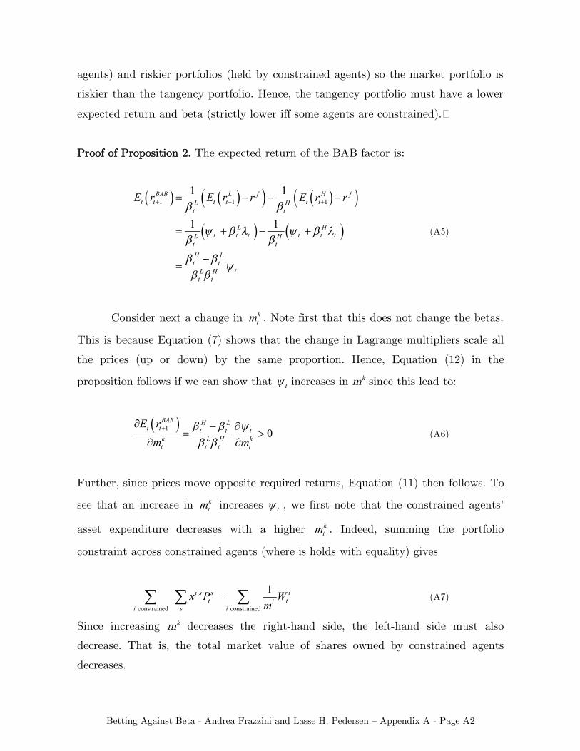
Proof of Proposition 2. The expected return of the BAB factor is:
1 1 11 1
1 1
BAB L f H ft t t t t tL H
t t
L Ht t t t t tL H
t tH Lt t
tL Ht t
E r E r r E r r
(A5)
Consider next a change in ktm . Note first that this does not change the betas.
This is because Equation (7) shows that the change in Lagrange multipliers scale all
the prices (up or down) by the same proportion. Hence, Equation (12) in the
proposition follows if we can show that t increases in mk since this lead to:
1 0BAB H L
t t t t tk L H kt t t t
E rm m
(A6)
Further, since prices move opposite required returns, Equation (11) then follows. To
see that an increase in ktm increases t , we first note that the constrained agents’
asset expenditure decreases with a higher ktm . Indeed, summing the portfolio
constraint across constrained agents (where is holds with equality) gives
,
constrained constrained
1i s s it ti
i s ix P W
m (A7)
Since increasing mk decreases the right-hand side, the left-hand side must also
decrease. That is, the total market value of shares owned by constrained agents
decreases.

Betting Against Beta - Andrea Frazzini and Lasse H. Pedersen – Appendix A - Page A3
Next, the constrained agents’ expenditure is decreasing in so must
increase:
constrained constrained' ' ' 0
ii it
t ti i
P xP x x P
(A8)
To see the last inequality, note first that clearly ' 0itP x
since all the prices
decrease by the same proportion (seen in Equation (7)) and the initial expenditure is
positive. The second term is also negative since
1 111
constrained constrained
1 11
constrained
1
* *1' ' 11 1
* *1' 11 1
*1
t t t ti f it t t tf i f
i i
t t t tf itf i f
i
t tf
E P x E P xP x E P r
r r
E P x E P xr
r r
E P xr
11
11 1
*1' 11
11 1 * ' *1 1
0
t tff
f
t t t tf f
E P xq r
r
q rE P x E P x
r r
where we have defined constrained
1ii
q
and used that constrained
i ii i
i i
since 0i for unconstrained agents. This completes the proof.
Proof of Proposition 3. Using the Equation (7) for the price, the sensitivity of with
respect to funding shocks can be calculated as
1/1
st
ts ft t
PP r
(A9)
which is the same for all securities s.

Betting Against Beta - Andrea Frazzini and Lasse H. Pedersen – Appendix A - Page A4
Intuitively, shocks that affect all securities the same way compress betas
towards one. This is seen most easily using long returns:
,log
1
1 1
log log
log * log 1 log
s s st t t
s f st t t t
r P P
E P x r P
(A10)
Hence, a higher variance of log 1 ftr increases all co-variances and variances
by the same amount, thus pushing betas – the ratio of covariance to market variance
– towards one.
The result is seen as follows when returns are computed as ratios:
1
1 1
*11 11
i iit t ti t
t i f it t t
E P xPrP r P
(A11)
First, we decompose returns into two parts:
1i it t tr x z (A12)
where
1
11
1
1 1/1 1
*11
t tf ft t
i it t ti
t t f it t
x Er r
E P xz E
r P
(A13)
When x is independent of z, the covariance between and security i and the market
M can be written as:
1 1
21 1 1
2 21 1 1 1 1 1
1 1 1
cov ( , ) cov ( , )
var ( ) ( ) ( )
var ( ) cov ( , )
i M i Mt t t t
i M i Mt t t
i M i Mt t t t t t
i M i Mt t t
r r x z x z
E x z z E x z E x z
x E x E z z E x E z E z
x E z z z z
(A14)
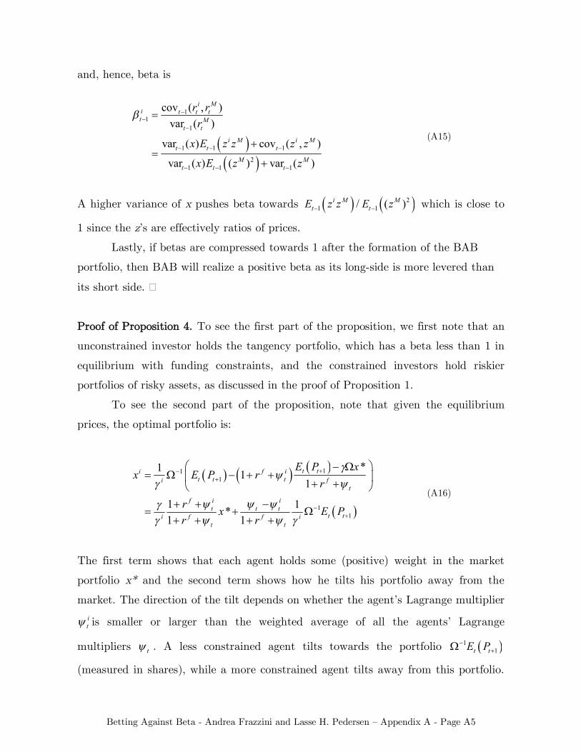
Betting Against Beta - Andrea Frazzini and Lasse H. Pedersen – Appendix A - Page A5
and, hence, beta is
11
1
1 1 1
21 1 1
cov ( , )var ( )
var ( ) cov ( , )
var ( ) ( ) var ( )
i Mi t t tt M
t t
i M i Mt t t
M Mt t t
r rr
x E z z z z
x E z z
(A15)
A higher variance of x pushes beta towards 21 1/ ( )i M M
t tE z z E z which is close to
1 since the z’s are effectively ratios of prices.
Lastly, if betas are compressed towards 1 after the formation of the BAB
portfolio, then BAB will realize a positive beta as its long-side is more levered than
its short side.
Proof of Proposition 4. To see the first part of the proposition, we first note that an
unconstrained investor holds the tangency portfolio, which has a beta less than 1 in
equilibrium with funding constraints, and the constrained investors hold riskier
portfolios of risky assets, as discussed in the proof of Proposition 1.
To see the second part of the proposition, note that given the equilibrium
prices, the optimal portfolio is:
111
11
*1 11
1 1*1 1
t ti f it t ti f
t
f i it t t
t ti f f it t
E P xx E P r
r
r x E Pr r
(A16)
The first term shows that each agent holds some (positive) weight in the market
portfolio x* and the second term shows how he tilts his portfolio away from the
market. The direction of the tilt depends on whether the agent’s Lagrange multiplier
it is smaller or larger than the weighted average of all the agents’ Lagrange
multipliers t . A less constrained agent tilts towards the portfolio 11t tE P
(measured in shares), while a more constrained agent tilts away from this portfolio.

Betting Against Beta - Andrea Frazzini and Lasse H. Pedersen – Appendix A - Page A6
Given the expression (13), we can write the variance-covariance matrix as
2 'M bb (A17)
where Σ=var(e) and 21var M
M tP . Using the Matrix Inversion Lemma (the
Sherman–Morrison–Woodbury formula), the tilt portfolio can be written as:
1 1 1 11 12 1
1 1 11 1 2 1
1 11
1''
1''
t t t tM
t t t tM
t t
E P bb E Pb b
E P bb E Pb b
E P y b
(A18)
where 1 2 11' / 't t My b E P b b is a scalar and 1 1
s kb b since s kb b
and s and k have the rows and columns in implying that 1 1
, ,s s s k
. So
everything else equal, a higher b leads to a lower weight in the tilt portfolio.
Finally, we note that security s also has a higher return beta than k since
1 1
1
cov( , )var
M i M Mi it t t tt ii M
tt t
P P P P bPP P
(A19)
and a higher bi means a lower price:
21 1* * ' *
1 1
i i it t t t Mi ii
tf i f i
t ti ii i
E P x E P x b b xP
r r
(A20)
Betting Against Beta - Andrea Frazzini and Lasse H. Pedersen – Appendix B - Page B1
Appendix B: Additional Empirical Results and Robustness Tests
Tables B1 to B7 and Figures B1 to B7 contain additional empirical results and
robustness tests.
- Table B1 reports returns of BAB portfolio in US and global equities using different
window lengths and different benchmark to estimate betas.
- Table B2 reports returns and factor loadings of US and Global BAB portfolios
- Table B3 and B4 report returns of US and Global BAB portfolios controlling for
idiosyncratic volatility. Idiosyncratic volatility is defined as the standard deviation
of the residuals in the rolling regression used to estimated betas. We use
conditional sorts: at the beginning of each calendar month stocks are ranked in
ascending order on the basis of their idiosyncratic volatility and assigned to one of
10 groups from low to high volatility. Within each volatility deciles, we assign
stocks to low and high beta portfolios and compute BAB returns. We report two
sets of results: controlling for the level of idiosyncratic volatility and the 1-month
change in the same measure.
- Table B5 reports returns of US and Global BAB portfolios controlling for size. Size
is defined as the market value of equity (in USD). We use conditional sorts: at the
beginning of each calendar month stocks are ranked in ascending order on the basis
of their market value of equity and assigned to one of 10 groups from small to
large based on NSYE breakpoints. Within each size deciles, we assign stocks to low
and high beta portfolios and compute BAB returns.
- Table B6 reports returns of US and Global BAB portfolios in different sample
periods
Betting Against Beta - Andrea Frazzini and Lasse H. Pedersen – Appendix B - Page B2
- Table B7 reports returns of BAB portfolios for all asset classes in different time
periods sorted by likelihood of binding credit constraints. At the beginning of each
calendar month, we rescale each return series to 10% annualized volatility using
rolling 3-year estimate up to moth t-1. We assign the Ted spread into three groups
(low, neutral and high) based on full sample breakpoints (top and bottom 1/3) and
report returns for each time period.
- Figure B1 plot the Sharpe ratio (annualized) of beta-sorted portfolios for all the
asset classes.
- Figures B2 to B7 reports calendar time returns of the BAB portfolios.
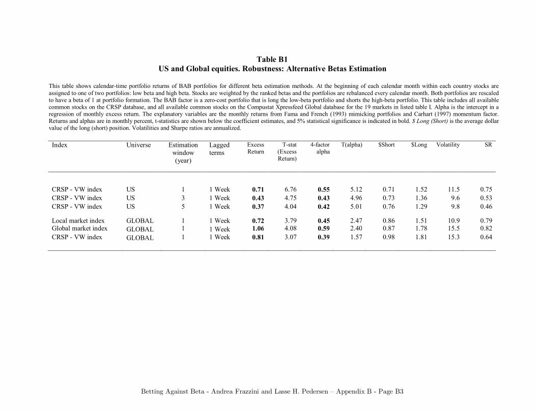
Betting Against Beta - Andrea Frazzini and Lasse H. Pedersen – Appendix B - Page B3
Table B1 US and Global equities. Robustness: Alternative Betas Estimation
This table shows calendar-time portfolio returns of BAB portfolios for different beta estimation methods. At the beginning of each calendar month within each country stocks are assigned to one of two portfolios: low beta and high beta. Stocks are weighted by the ranked betas and the portfolios are rebalanced every calendar month. Both portfolios are rescaled to have a beta of 1 at portfolio formation. The BAB factor is a zero-cost portfolio that is long the low-beta portfolio and shorts the high-beta portfolio. This table includes all available common stocks on the CRSP database, and all available common stocks on the Compustat Xpressfeed Global database for the 19 markets in listed table I. Alpha is the intercept in a regression of monthly excess return. The explanatory variables are the monthly returns from Fama and French (1993) mimicking portfolios and Carhart (1997) momentum factor. Returns and alphas are in monthly percent, t-statistics are shown below the coefficient estimates, and 5% statistical significance is indicated in bold. $ Long (Short) is the average dollar value of the long (short) position. Volatilities and Sharpe ratios are annualized. Index Universe Estimation
window (year)
Lagged terms
Excess Return
T-stat (Excess Return)
4-factor alpha
T(alpha) $Short $Long Volatility SR
CRSP - VW index US 1 1 Week 0.71 6.76 0.55 5.12 0.71 1.52 11.5 0.75 CRSP - VW index US 3 1 Week 0.43 4.75 0.43 4.96 0.73 1.36 9.6 0.53 CRSP - VW index US 5 1 Week 0.37 4.04 0.42 5.01 0.76 1.29 9.8 0.46
Local market index GLOBAL 1 1 Week 0.72 3.79 0.45 2.47 0.86 1.51 10.9 0.79 Global market index GLOBAL 1 1 Week 1.06 4.08 0.59 2.40 0.87 1.78 15.5 0.82 CRSP - VW index GLOBAL 1 1 Week 0.81 3.07 0.39 1.57 0.98 1.81 15.3 0.64
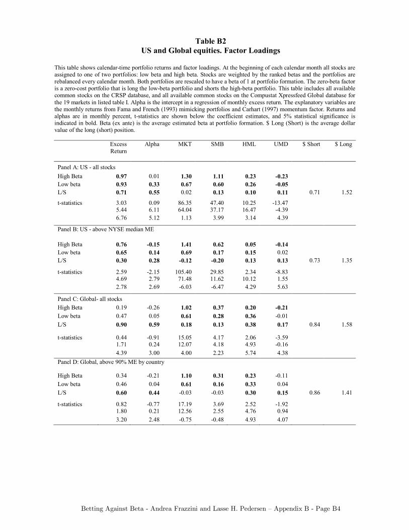
Betting Against Beta - Andrea Frazzini and Lasse H. Pedersen – Appendix B - Page B4
Table B2 US and Global equities. Factor Loadings
This table shows calendar-time portfolio returns and factor loadings. At the beginning of each calendar month all stocks are assigned to one of two portfolios: low beta and high beta. Stocks are weighted by the ranked betas and the portfolios are rebalanced every calendar month. Both portfolios are rescaled to have a beta of 1 at portfolio formation. The zero-beta factor is a zero-cost portfolio that is long the low-beta portfolio and shorts the high-beta portfolio. This table includes all available common stocks on the CRSP database, and all available common stocks on the Compustat Xpressfeed Global database for the 19 markets in listed table I. Alpha is the intercept in a regression of monthly excess return. The explanatory variables are the monthly returns from Fama and French (1993) mimicking portfolios and Carhart (1997) momentum factor. Returns and alphas are in monthly percent, t-statistics are shown below the coefficient estimates, and 5% statistical significance is indicated in bold. Beta (ex ante) is the average estimated beta at portfolio formation. $ Long (Short) is the average dollar value of the long (short) position.
Excess Return
Alpha MKT SMB HML UMD $ Short $ Long
Panel A: US - all stocks High Beta 0.97 0.01 1.30 1.11 0.23 -0.23 Low beta 0.93 0.33 0.67 0.60 0.26 -0.05 L/S 0.71 0.55 0.02 0.13 0.10 0.11 0.71 1.52
t-statistics 3.03 0.09 86.35 47.40 10.25 -13.47 5.44 6.11 64.04 37.17 16.47 -4.39
6.76 5.12 1.13 3.99 3.14 4.39
Panel B: US - above NYSE median ME
High Beta 0.76 -0.15 1.41 0.62 0.05 -0.14 Low beta 0.65 0.14 0.69 0.17 0.15 0.02 L/S 0.30 0.28 -0.12 -0.20 0.13 0.13 0.73 1.35
t-statistics 2.59 -2.15 105.40 29.85 2.34 -8.83 4.69 2.79 71.48 11.62 10.12 1.55 2.78 2.69 -6.03 -6.47 4.29 5.63 Panel C: Global- all stocks High Beta 0.19 -0.26 1.02 0.37 0.20 -0.21 Low beta 0.47 0.05 0.61 0.28 0.36 -0.01 L/S 0.90 0.59 0.18 0.13 0.38 0.17 0.84 1.58
t-statistics 0.44 -0.91 15.05 4.17 2.06 -3.59 1.71 0.24 12.07 4.18 4.93 -0.16 4.39 3.00 4.00 2.23 5.74 4.38 Panel D: Global, above 90% ME by country
High Beta 0.34 -0.21 1.10 0.31 0.23 -0.11 Low beta 0.46 0.04 0.61 0.16 0.33 0.04 L/S 0.60 0.44 -0.03 -0.03 0.30 0.15 0.86 1.41
t-statistics 0.82 -0.77 17.19 3.69 2.52 -1.92 1.80 0.21 12.56 2.55 4.76 0.94 3.20 2.48 -0.75 -0.48 4.93 4.07
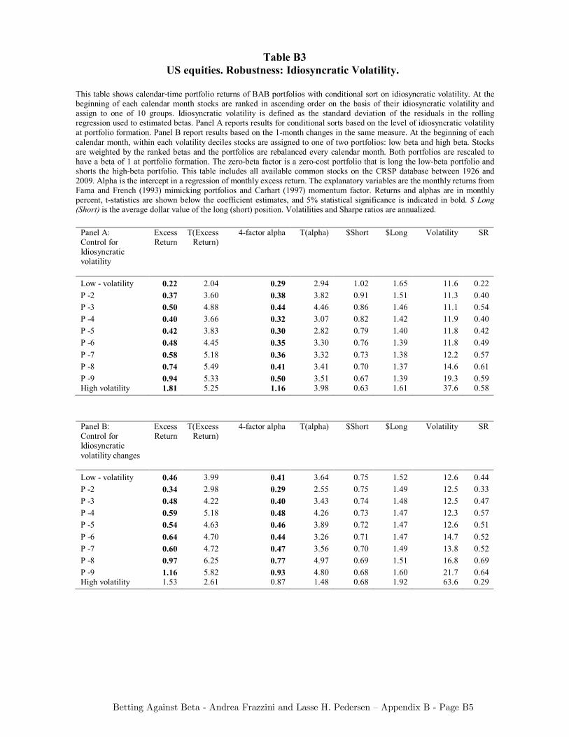
Betting Against Beta - Andrea Frazzini and Lasse H. Pedersen – Appendix B - Page B5
Table B3 US equities. Robustness: Idiosyncratic Volatility.
This table shows calendar-time portfolio returns of BAB portfolios with conditional sort on idiosyncratic volatility. At the beginning of each calendar month stocks are ranked in ascending order on the basis of their idiosyncratic volatility and assign to one of 10 groups. Idiosyncratic volatility is defined as the standard deviation of the residuals in the rolling regression used to estimated betas. Panel A reports results for conditional sorts based on the level of idiosyncratic volatility at portfolio formation. Panel B report results based on the 1-month changes in the same measure. At the beginning of each calendar month, within each volatility deciles stocks are assigned to one of two portfolios: low beta and high beta. Stocks are weighted by the ranked betas and the portfolios are rebalanced every calendar month. Both portfolios are rescaled to have a beta of 1 at portfolio formation. The zero-beta factor is a zero-cost portfolio that is long the low-beta portfolio and shorts the high-beta portfolio. This table includes all available common stocks on the CRSP database between 1926 and 2009. Alpha is the intercept in a regression of monthly excess return. The explanatory variables are the monthly returns from Fama and French (1993) mimicking portfolios and Carhart (1997) momentum factor. Returns and alphas are in monthly percent, t-statistics are shown below the coefficient estimates, and 5% statistical significance is indicated in bold. $ Long (Short) is the average dollar value of the long (short) position. Volatilities and Sharpe ratios are annualized.
Panel A: Control for Idiosyncratic volatility
Excess Return
T(Excess Return)
4-factor alpha T(alpha) $Short $Long Volatility SR
Low - volatility 0.22 2.04 0.29 2.94 1.02 1.65 11.6 0.22 P -2 0.37 3.60 0.38 3.82 0.91 1.51 11.3 0.40 P -3 0.50 4.88 0.44 4.46 0.86 1.46 11.1 0.54 P -4 0.40 3.66 0.32 3.07 0.82 1.42 11.9 0.40 P -5 0.42 3.83 0.30 2.82 0.79 1.40 11.8 0.42 P -6 0.48 4.45 0.35 3.30 0.76 1.39 11.8 0.49 P -7 0.58 5.18 0.36 3.32 0.73 1.38 12.2 0.57 P -8 0.74 5.49 0.41 3.41 0.70 1.37 14.6 0.61 P -9 0.94 5.33 0.50 3.51 0.67 1.39 19.3 0.59 High volatility 1.81 5.25 1.16 3.98 0.63 1.61 37.6 0.58
Panel B: Control for Idiosyncratic volatility changes
Excess Return
T(Excess Return)
4-factor alpha T(alpha) $Short $Long Volatility SR
Low - volatility 0.46 3.99 0.41 3.64 0.75 1.52 12.6 0.44 P -2 0.34 2.98 0.29 2.55 0.75 1.49 12.5 0.33 P -3 0.48 4.22 0.40 3.43 0.74 1.48 12.5 0.47 P -4 0.59 5.18 0.48 4.26 0.73 1.47 12.3 0.57 P -5 0.54 4.63 0.46 3.89 0.72 1.47 12.6 0.51 P -6 0.64 4.70 0.44 3.26 0.71 1.47 14.7 0.52 P -7 0.60 4.72 0.47 3.56 0.70 1.49 13.8 0.52 P -8 0.97 6.25 0.77 4.97 0.69 1.51 16.8 0.69 P -9 1.16 5.82 0.93 4.80 0.68 1.60 21.7 0.64 High volatility 1.53 2.61 0.87 1.48 0.68 1.92 63.6 0.29
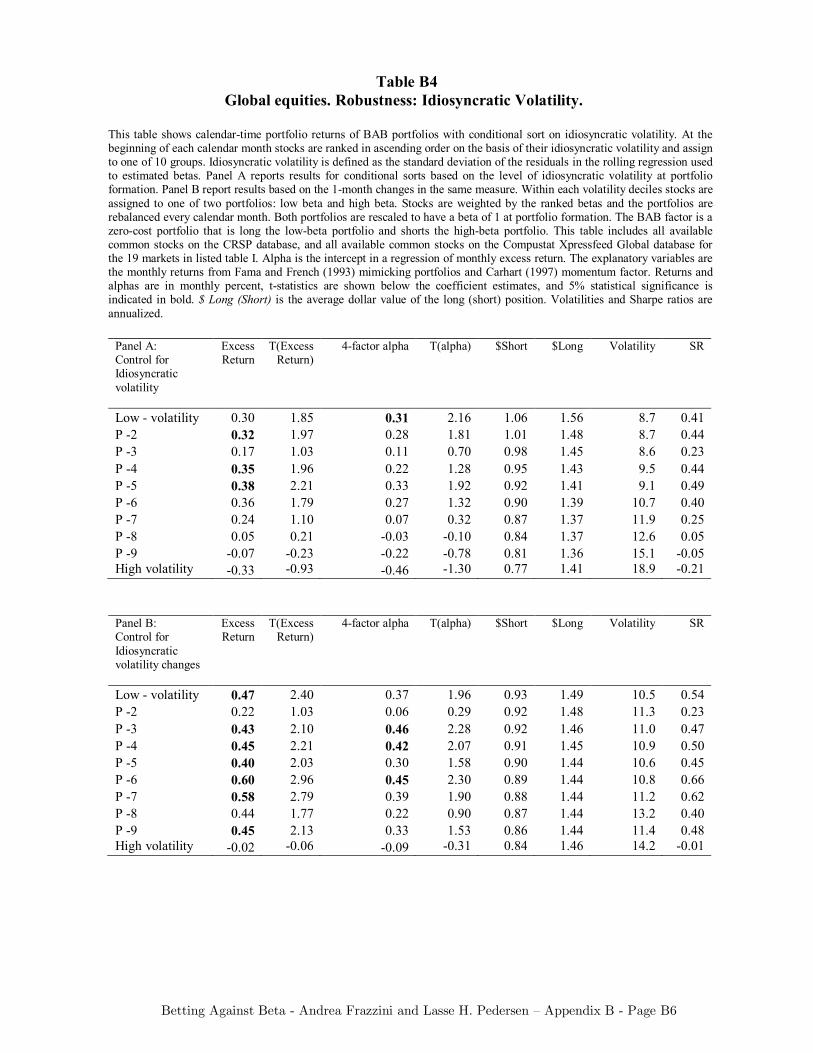
Betting Against Beta - Andrea Frazzini and Lasse H. Pedersen – Appendix B - Page B6
Table B4 Global equities. Robustness: Idiosyncratic Volatility.
This table shows calendar-time portfolio returns of BAB portfolios with conditional sort on idiosyncratic volatility. At the beginning of each calendar month stocks are ranked in ascending order on the basis of their idiosyncratic volatility and assign to one of 10 groups. Idiosyncratic volatility is defined as the standard deviation of the residuals in the rolling regression used to estimated betas. Panel A reports results for conditional sorts based on the level of idiosyncratic volatility at portfolio formation. Panel B report results based on the 1-month changes in the same measure. Within each volatility deciles stocks are assigned to one of two portfolios: low beta and high beta. Stocks are weighted by the ranked betas and the portfolios are rebalanced every calendar month. Both portfolios are rescaled to have a beta of 1 at portfolio formation. The BAB factor is a zero-cost portfolio that is long the low-beta portfolio and shorts the high-beta portfolio. This table includes all available common stocks on the CRSP database, and all available common stocks on the Compustat Xpressfeed Global database for the 19 markets in listed table I. Alpha is the intercept in a regression of monthly excess return. The explanatory variables are the monthly returns from Fama and French (1993) mimicking portfolios and Carhart (1997) momentum factor. Returns and alphas are in monthly percent, t-statistics are shown below the coefficient estimates, and 5% statistical significance is indicated in bold. $ Long (Short) is the average dollar value of the long (short) position. Volatilities and Sharpe ratios are annualized.
Panel A: Control for Idiosyncratic volatility
Excess Return
T(Excess Return)
4-factor alpha T(alpha) $Short $Long Volatility SR
Low - volatility 0.30 1.85 0.31 2.16 1.06 1.56 8.7 0.41 P -2 0.32 1.97 0.28 1.81 1.01 1.48 8.7 0.44 P -3 0.17 1.03 0.11 0.70 0.98 1.45 8.6 0.23 P -4 0.35 1.96 0.22 1.28 0.95 1.43 9.5 0.44 P -5 0.38 2.21 0.33 1.92 0.92 1.41 9.1 0.49 P -6 0.36 1.79 0.27 1.32 0.90 1.39 10.7 0.40 P -7 0.24 1.10 0.07 0.32 0.87 1.37 11.9 0.25 P -8 0.05 0.21 -0.03 -0.10 0.84 1.37 12.6 0.05 P -9 -0.07 -0.23 -0.22 -0.78 0.81 1.36 15.1 -0.05 High volatility -0.33 -0.93 -0.46 -1.30 0.77 1.41 18.9 -0.21
Panel B: Control for Idiosyncratic volatility changes
Excess Return
T(Excess Return)
4-factor alpha T(alpha) $Short $Long Volatility SR
Low - volatility 0.47 2.40 0.37 1.96 0.93 1.49 10.5 0.54 P -2 0.22 1.03 0.06 0.29 0.92 1.48 11.3 0.23 P -3 0.43 2.10 0.46 2.28 0.92 1.46 11.0 0.47 P -4 0.45 2.21 0.42 2.07 0.91 1.45 10.9 0.50 P -5 0.40 2.03 0.30 1.58 0.90 1.44 10.6 0.45 P -6 0.60 2.96 0.45 2.30 0.89 1.44 10.8 0.66 P -7 0.58 2.79 0.39 1.90 0.88 1.44 11.2 0.62 P -8 0.44 1.77 0.22 0.90 0.87 1.44 13.2 0.40 P -9 0.45 2.13 0.33 1.53 0.86 1.44 11.4 0.48 High volatility -0.02 -0.06 -0.09 -0.31 0.84 1.46 14.2 -0.01
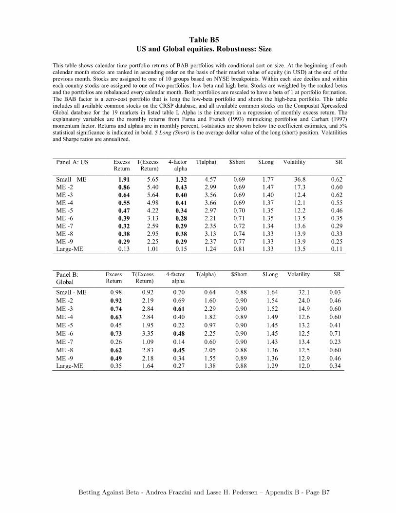
Betting Against Beta - Andrea Frazzini and Lasse H. Pedersen – Appendix B - Page B7
Table B5 US and Global equities. Robustness: Size
This table shows calendar-time portfolio returns of BAB portfolios with conditional sort on size. At the beginning of each calendar month stocks are ranked in ascending order on the basis of their market value of equity (in USD) at the end of the previous month. Stocks are assigned to one of 10 groups based on NYSE breakpoints. Within each size deciles and within each country stocks are assigned to one of two portfolios: low beta and high beta. Stocks are weighted by the ranked betas and the portfolios are rebalanced every calendar month. Both portfolios are rescaled to have a beta of 1 at portfolio formation. The BAB factor is a zero-cost portfolio that is long the low-beta portfolio and shorts the high-beta portfolio. This table includes all available common stocks on the CRSP database, and all available common stocks on the Compustat Xpressfeed Global database for the 19 markets in listed table I. Alpha is the intercept in a regression of monthly excess return. The explanatory variables are the monthly returns from Fama and French (1993) mimicking portfolios and Carhart (1997) momentum factor. Returns and alphas are in monthly percent, t-statistics are shown below the coefficient estimates, and 5% statistical significance is indicated in bold. $ Long (Short) is the average dollar value of the long (short) position. Volatilities and Sharpe ratios are annualized.
Panel A: US Excess Return
T(Excess Return)
4-factor alpha
T(alpha) $Short $Long Volatility SR
Small - ME 1.91 5.65 1.32 4.57 0.69 1.77 36.8 0.62 ME -2 0.86 5.40 0.43 2.99 0.69 1.47 17.3 0.60 ME -3 0.64 5.64 0.40 3.56 0.69 1.40 12.4 0.62 ME -4 0.55 4.98 0.41 3.66 0.69 1.37 12.1 0.55 ME -5 0.47 4.22 0.34 2.97 0.70 1.35 12.2 0.46 ME -6 0.39 3.13 0.28 2.21 0.71 1.35 13.5 0.35 ME -7 0.32 2.59 0.29 2.35 0.72 1.34 13.6 0.29 ME -8 0.38 2.95 0.38 3.13 0.74 1.33 13.9 0.33 ME -9 0.29 2.25 0.29 2.37 0.77 1.33 13.9 0.25 Large-ME 0.13 1.01 0.15 1.24 0.81 1.33 13.5 0.11
Panel B: Global
Excess Return
T(Excess Return)
4-factor alpha
T(alpha) $Short $Long Volatility SR
Small - ME 0.98 0.92 0.70 0.64 0.88 1.64 32.1 0.03 ME -2 0.92 2.19 0.69 1.60 0.90 1.54 24.0 0.46 ME -3 0.74 2.84 0.61 2.29 0.90 1.52 14.9 0.60 ME -4 0.63 2.84 0.40 1.82 0.89 1.49 12.6 0.60 ME -5 0.45 1.95 0.22 0.97 0.90 1.45 13.2 0.41 ME -6 0.73 3.35 0.48 2.25 0.90 1.45 12.5 0.71 ME -7 0.26 1.09 0.14 0.60 0.90 1.43 13.4 0.23 ME -8 0.62 2.83 0.45 2.05 0.88 1.36 12.5 0.60 ME -9 0.49 2.18 0.34 1.55 0.89 1.36 12.9 0.46 Large-ME 0.35 1.64 0.27 1.38 0.88 1.29 12.0 0.34
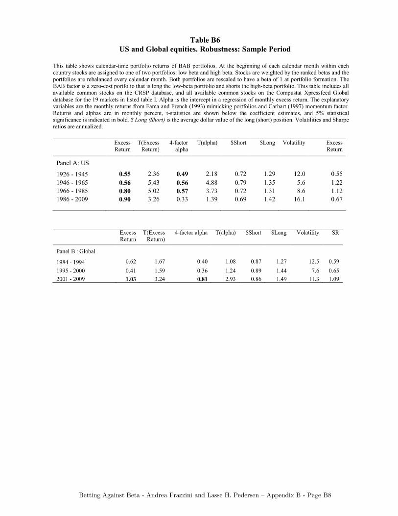
Betting Against Beta - Andrea Frazzini and Lasse H. Pedersen – Appendix B - Page B8
Table B6 US and Global equities. Robustness: Sample Period
This table shows calendar-time portfolio returns of BAB portfolios. At the beginning of each calendar month within each country stocks are assigned to one of two portfolios: low beta and high beta. Stocks are weighted by the ranked betas and the portfolios are rebalanced every calendar month. Both portfolios are rescaled to have a beta of 1 at portfolio formation. The BAB factor is a zero-cost portfolio that is long the low-beta portfolio and shorts the high-beta portfolio. This table includes all available common stocks on the CRSP database, and all available common stocks on the Compustat Xpressfeed Global database for the 19 markets in listed table I. Alpha is the intercept in a regression of monthly excess return. The explanatory variables are the monthly returns from Fama and French (1993) mimicking portfolios and Carhart (1997) momentum factor. Returns and alphas are in monthly percent, t-statistics are shown below the coefficient estimates, and 5% statistical significance is indicated in bold. $ Long (Short) is the average dollar value of the long (short) position. Volatilities and Sharpe ratios are annualized.
Excess Return
T(Excess Return)
4-factor alpha
T(alpha) $Short $Long Volatility Excess Return
Panel A: US 1926 - 1945 0.55 2.36 0.49 2.18 0.72 1.29 12.0 0.55 1946 - 1965 0.56 5.43 0.56 4.88 0.79 1.35 5.6 1.22 1966 - 1985 0.80 5.02 0.57 3.73 0.72 1.31 8.6 1.12 1986 - 2009 0.90 3.26 0.33 1.39 0.69 1.42 16.1 0.67
Excess Return
T(Excess Return)
4-factor alpha T(alpha) $Short $Long Volatility SR
Panel B : Global 1984 - 1994 0.62 1.67 0.40 1.08 0.87 1.27 12.5 0.59 1995 - 2000 0.41 1.59 0.36 1.24 0.89 1.44 7.6 0.65 2001 - 2009 1.03 3.24 0.81 2.93 0.86 1.49 11.3 1.09
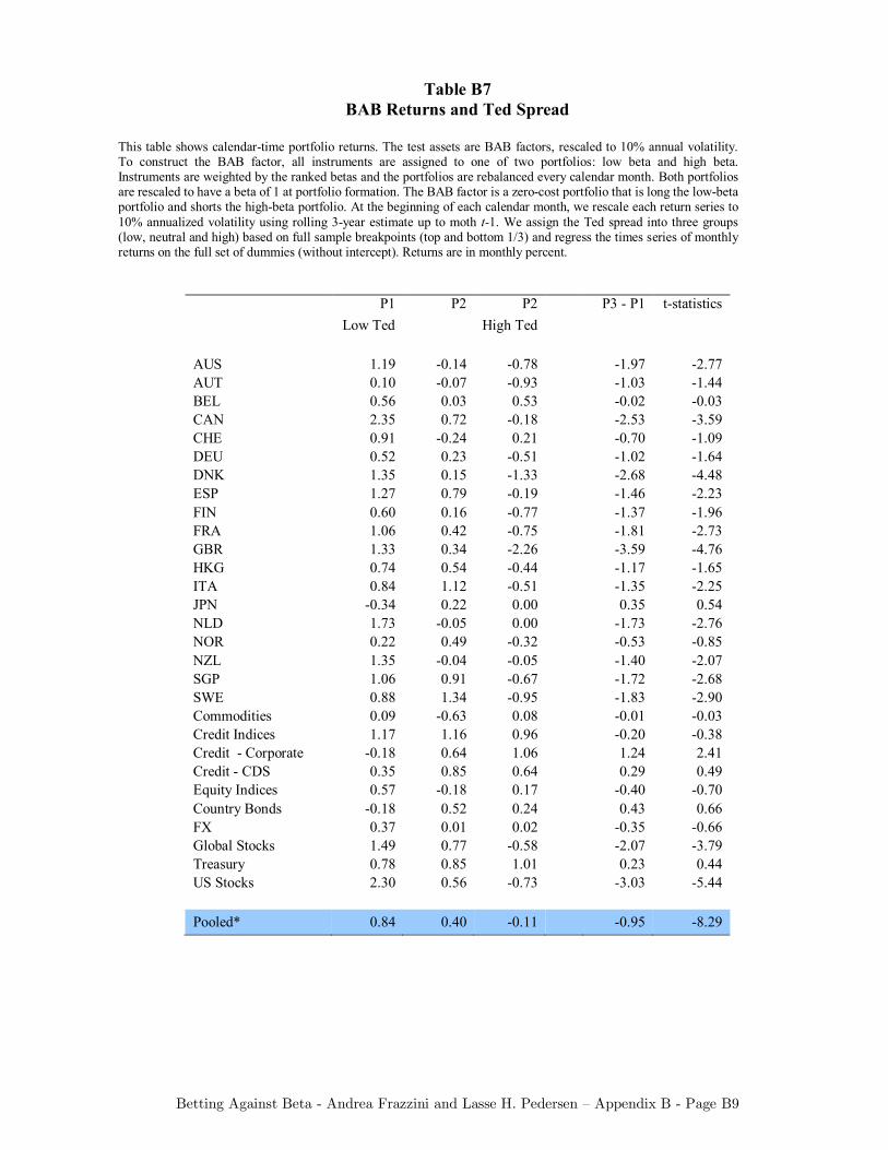
Betting Against Beta - Andrea Frazzini and Lasse H. Pedersen – Appendix B - Page B9
Table B7 BAB Returns and Ted Spread
This table shows calendar-time portfolio returns. The test assets are BAB factors, rescaled to 10% annual volatility. To construct the BAB factor, all instruments are assigned to one of two portfolios: low beta and high beta. Instruments are weighted by the ranked betas and the portfolios are rebalanced every calendar month. Both portfolios are rescaled to have a beta of 1 at portfolio formation. The BAB factor is a zero-cost portfolio that is long the low-beta portfolio and shorts the high-beta portfolio. At the beginning of each calendar month, we rescale each return series to 10% annualized volatility using rolling 3-year estimate up to moth t-1. We assign the Ted spread into three groups (low, neutral and high) based on full sample breakpoints (top and bottom 1/3) and regress the times series of monthly returns on the full set of dummies (without intercept). Returns are in monthly percent.
P1 P2 P2 P3 - P1 t-statistics Low Ted High Ted
AUS 1.19 -0.14 -0.78 -1.97 -2.77 AUT 0.10 -0.07 -0.93 -1.03 -1.44 BEL 0.56 0.03 0.53 -0.02 -0.03 CAN 2.35 0.72 -0.18 -2.53 -3.59 CHE 0.91 -0.24 0.21 -0.70 -1.09 DEU 0.52 0.23 -0.51 -1.02 -1.64 DNK 1.35 0.15 -1.33 -2.68 -4.48 ESP 1.27 0.79 -0.19 -1.46 -2.23 FIN 0.60 0.16 -0.77 -1.37 -1.96 FRA 1.06 0.42 -0.75 -1.81 -2.73 GBR 1.33 0.34 -2.26 -3.59 -4.76 HKG 0.74 0.54 -0.44 -1.17 -1.65 ITA 0.84 1.12 -0.51 -1.35 -2.25 JPN -0.34 0.22 0.00 0.35 0.54 NLD 1.73 -0.05 0.00 -1.73 -2.76 NOR 0.22 0.49 -0.32 -0.53 -0.85 NZL 1.35 -0.04 -0.05 -1.40 -2.07 SGP 1.06 0.91 -0.67 -1.72 -2.68 SWE 0.88 1.34 -0.95 -1.83 -2.90 Commodities 0.09 -0.63 0.08 -0.01 -0.03 Credit Indices 1.17 1.16 0.96 -0.20 -0.38 Credit - Corporate -0.18 0.64 1.06 1.24 2.41 Credit - CDS 0.35 0.85 0.64 0.29 0.49 Equity Indices 0.57 -0.18 0.17 -0.40 -0.70 Country Bonds -0.18 0.52 0.24 0.43 0.66 FX 0.37 0.01 0.02 -0.35 -0.66 Global Stocks 1.49 0.77 -0.58 -2.07 -3.79 Treasury 0.78 0.85 1.01 0.23 0.44 US Stocks 2.30 0.56 -0.73 -3.03 -5.44 Pooled* 0.84 0.40 -0.11 -0.95 -8.29
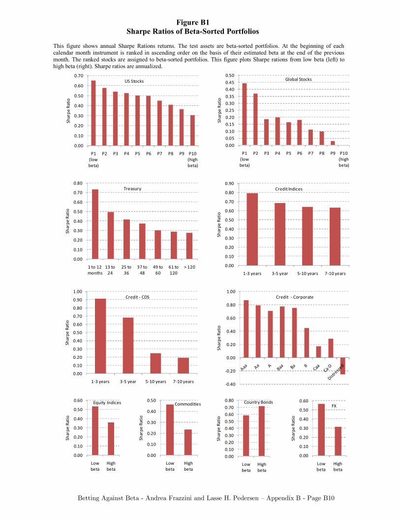
Betting Against Beta - Andrea Frazzini and Lasse H. Pedersen – Appendix B - Page B10
Figure B1 Sharpe Ratios of Beta-Sorted Portfolios
This figure shows annual Sharpe Rations returns. The test assets are beta-sorted portfolios. At the beginning of each calendar month instrument is ranked in ascending order on the basis of their estimated beta at the end of the previous month. The ranked stocks are assigned to beta-sorted portfolios. This figure plots Sharpe rations from low beta (left) to high beta (right). Sharpe ratios are annualized.
0.00
0.10
0.20
0.30
0.40
0.50
0.60
0.70
P1 (low beta)
P2 P3 P4 P5 P6 P7 P8 P9 P10 (high beta)
Shar
pe R
atio
US Stocks
0.00
0.05
0.10
0.15
0.20
0.25
0.30
0.35
0.40
0.45
0.50
P1 (low beta)
P2 P3 P4 P5 P6 P7 P8 P9 P10 (high beta)
Shar
pe R
atio
Global Stocks
0.00
0.10
0.20
0.30
0.40
0.50
0.60
0.70
0.80
1 to 12 months
13 to 24
25 to 36
37 to 48
49 to 60
61 to 120
> 120
Shar
pe R
atio
Treasury
0.00
0.10
0.20
0.30
0.40
0.50
0.60
0.70
0.80
0.90
1-3 years 3-5 year 5-10 years 7-10 years
Shar
pe R
atio
Credit Indices
0.00
0.10
0.20
0.30
0.40
0.50
0.60
0.70
0.80
0.90
1.00
1-3 years 3-5 year 5-10 years 7-10 years
Shar
pe R
atio
Credit - CDS
-0.40
-0.20
0.00
0.20
0.40
0.60
0.80
1.00
Shar
pe R
atio
Credit - Corporate
0.00
0.10
0.20
0.30
0.40
0.50
0.60
Low beta
High beta
Shar
pe R
atio
Equity Indices
0.00
0.10
0.20
0.30
0.40
0.50
Low beta
High beta
Shar
pe R
atio
Commodities
0.00
0.10
0.20
0.30
0.40
0.50
0.60
Low beta
High beta
Shar
pe R
atio
FX
0.00
0.10
0.20
0.30
0.40
0.50
0.60
0.70
0.80
Low beta
High beta
Shar
pe R
atio
Country Bonds
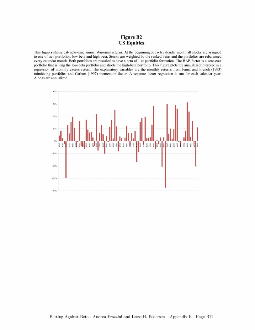
Betting Against Beta - Andrea Frazzini and Lasse H. Pedersen – Appendix B - Page B11
Figure B2 US Equities
This figures shows calendar-time annual abnormal returns. At the beginning of each calendar month all stocks are assigned to one of two portfolios: low beta and high beta. Stocks are weighted by the ranked betas and the portfolios are rebalanced every calendar month. Both portfolios are rescaled to have a beta of 1 at portfolio formation. The BAB factor is a zero-cost portfolio that is long the low-beta portfolio and shorts the high-beta portfolio. This figure plots the annualized intercept in a regression of monthly excess return. The explanatory variables are the monthly returns from Fama and French (1993) mimicking portfolios and Carhart (1997) momentum factor. A separate factor regression is run for each calendar year. Alphas are annualized.
-40%
-30%
-20%
-10%
0%
10%
20%
30%
40%
1927
1929
1931
1933
1935
1937
1939
1941
1943
1945
1947
1949
1951
1953
1955
1957
1959
1961
1963
1965
1967
1969
1971
1973
1975
1977
1979
1981
1983
1985
1987
1989
1991
1993
1995
1997
1999
2001
2003
2005
2007
2009
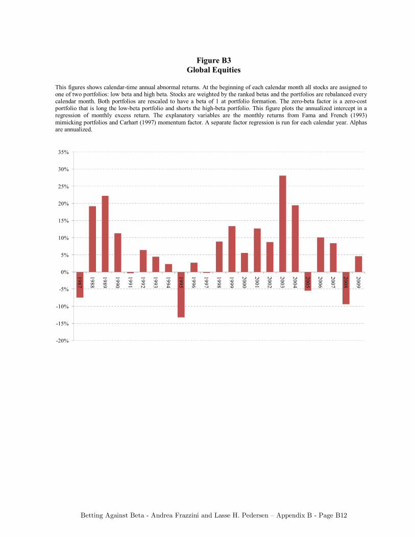
Betting Against Beta - Andrea Frazzini and Lasse H. Pedersen – Appendix B - Page B12
Figure B3 Global Equities
This figures shows calendar-time annual abnormal returns. At the beginning of each calendar month all stocks are assigned to one of two portfolios: low beta and high beta. Stocks are weighted by the ranked betas and the portfolios are rebalanced every calendar month. Both portfolios are rescaled to have a beta of 1 at portfolio formation. The zero-beta factor is a zero-cost portfolio that is long the low-beta portfolio and shorts the high-beta portfolio. This figure plots the annualized intercept in a regression of monthly excess return. The explanatory variables are the monthly returns from Fama and French (1993) mimicking portfolios and Carhart (1997) momentum factor. A separate factor regression is run for each calendar year. Alphas are annualized.
-20%
-15%
-10%
-5%
0%
5%
10%
15%
20%
25%
30%
35%
1987
1988
1989
1990
1991
1992
1993
1994
1995
1996
1997
1998
1999
2000
2001
2002
2003
2004
2005
2006
2007
2008
2009
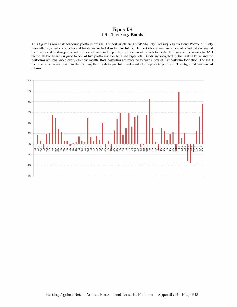
Betting Against Beta - Andrea Frazzini and Lasse H. Pedersen – Appendix B - Page B13
Figure B4 US - Treasury Bonds
This figures shows calendar-time portfolio returns. The test assets are CRSP Monthly Treasury - Fama Bond Portfolios. Only non-callable, non-flower notes and bonds are included in the portfolios. The portfolio returns are an equal weighted average of the unadjusted holding period return for each bond in the portfolios in excess of the risk free rate. To construct the zero-beta BAB factor, all bonds are assigned to one of two portfolios: low beta and high beta. Bonds are weighted by the ranked betas and the portfolios are rebalanced every calendar month. Both portfolios are rescaled to have a beta of 1 at portfolio formation. The BAB factor is a zero-cost portfolio that is long the low-beta portfolio and shorts the high-beta portfolio. This figure shows annual returns.
-6%
-4%
-2%
0%
2%
4%
6%
8%
10%
12%
1952195319541955195619571958195919601961196219631964196519661967196819691970197119721973197419751976197719781979198019811982198319841985198619871988198919901991199219931994199519961997199819992000200120022003200420052006200720082009
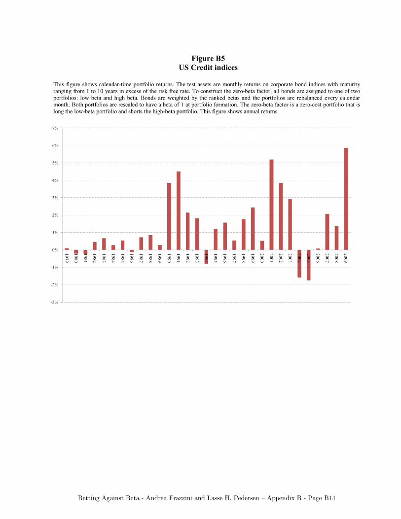
Betting Against Beta - Andrea Frazzini and Lasse H. Pedersen – Appendix B - Page B14
Figure B5 US Credit indices
This figure shows calendar-time portfolio returns. The test assets are monthly returns on corporate bond indices with maturity ranging from 1 to 10 years in excess of the risk free rate. To construct the zero-beta factor, all bonds are assigned to one of two portfolios: low beta and high beta. Bonds are weighted by the ranked betas and the portfolios are rebalanced every calendar month. Both portfolios are rescaled to have a beta of 1 at portfolio formation. The zero-beta factor is a zero-cost portfolio that is long the low-beta portfolio and shorts the high-beta portfolio. This figure shows annual returns.
-3%
-2%
-1%
0%
1%
2%
3%
4%
5%
6%
7%
1979
1980
1981
1982
1983
1984
1985
1986
1987
1988
1989
1990
1991
1992
1993
1994
1995
1996
1997
1998
1999
2000
2001
2002
2003
2004
2005
2006
2007
2008
2009
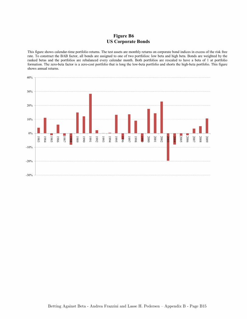
Betting Against Beta - Andrea Frazzini and Lasse H. Pedersen – Appendix B - Page B15
Figure B6 US Corporate Bonds
This figure shows calendar-time portfolio returns. The test assets are monthly returns on corporate bond indices in excess of the risk free rate. To construct the BAB factor, all bonds are assigned to one of two portfolios: low beta and high beta. Bonds are weighted by the ranked betas and the portfolios are rebalanced every calendar month. Both portfolios are rescaled to have a beta of 1 at portfolio formation. The zero-beta factor is a zero-cost portfolio that is long the low-beta portfolio and shorts the high-beta portfolio. This figure shows annual returns.
-30%
-20%
-10%
0%
10%
20%
30%
40%
1983
1984
1985
1986
1987
1988
1989
1990
1991
1992
1993
1994
1995
1996
1997
1998
1999
2000
2001
2002
2003
2004
2005
2006
2007
2008
2009
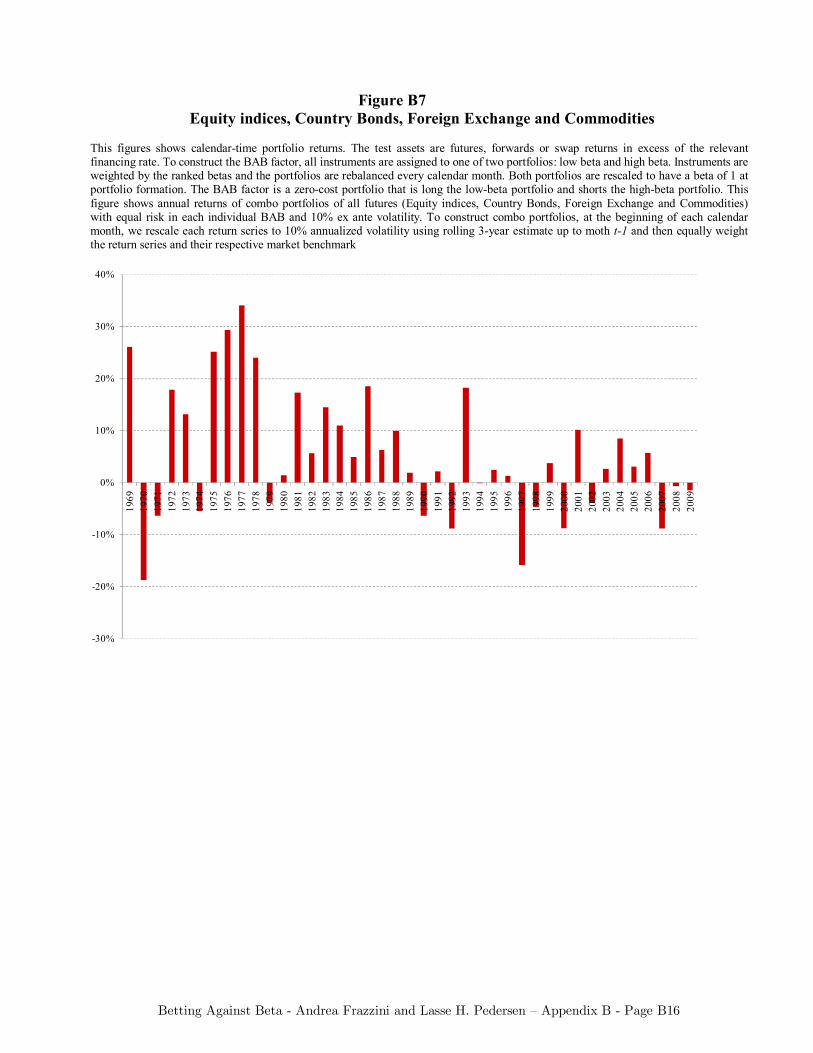
Betting Against Beta - Andrea Frazzini and Lasse H. Pedersen – Appendix B - Page B16
Figure B7 Equity indices, Country Bonds, Foreign Exchange and Commodities
This figures shows calendar-time portfolio returns. The test assets are futures, forwards or swap returns in excess of the relevant financing rate. To construct the BAB factor, all instruments are assigned to one of two portfolios: low beta and high beta. Instruments are weighted by the ranked betas and the portfolios are rebalanced every calendar month. Both portfolios are rescaled to have a beta of 1 at portfolio formation. The BAB factor is a zero-cost portfolio that is long the low-beta portfolio and shorts the high-beta portfolio. This figure shows annual returns of combo portfolios of all futures (Equity indices, Country Bonds, Foreign Exchange and Commodities) with equal risk in each individual BAB and 10% ex ante volatility. To construct combo portfolios, at the beginning of each calendar month, we rescale each return series to 10% annualized volatility using rolling 3-year estimate up to moth t-1 and then equally weight the return series and their respective market benchmark
-30%
-20%
-10%
0%
10%
20%
30%
40%
1969
1970
1971
1972
1973
1974
1975
1976
1977
1978
1979
1980
1981
1982
1983
1984
1985
1986
1987
1988
1989
1990
1991
1992
1993
1994
1995
1996
1997
1998
1999
2000
2001
2002
2003
2004
2005
2006
2007
2008
2009
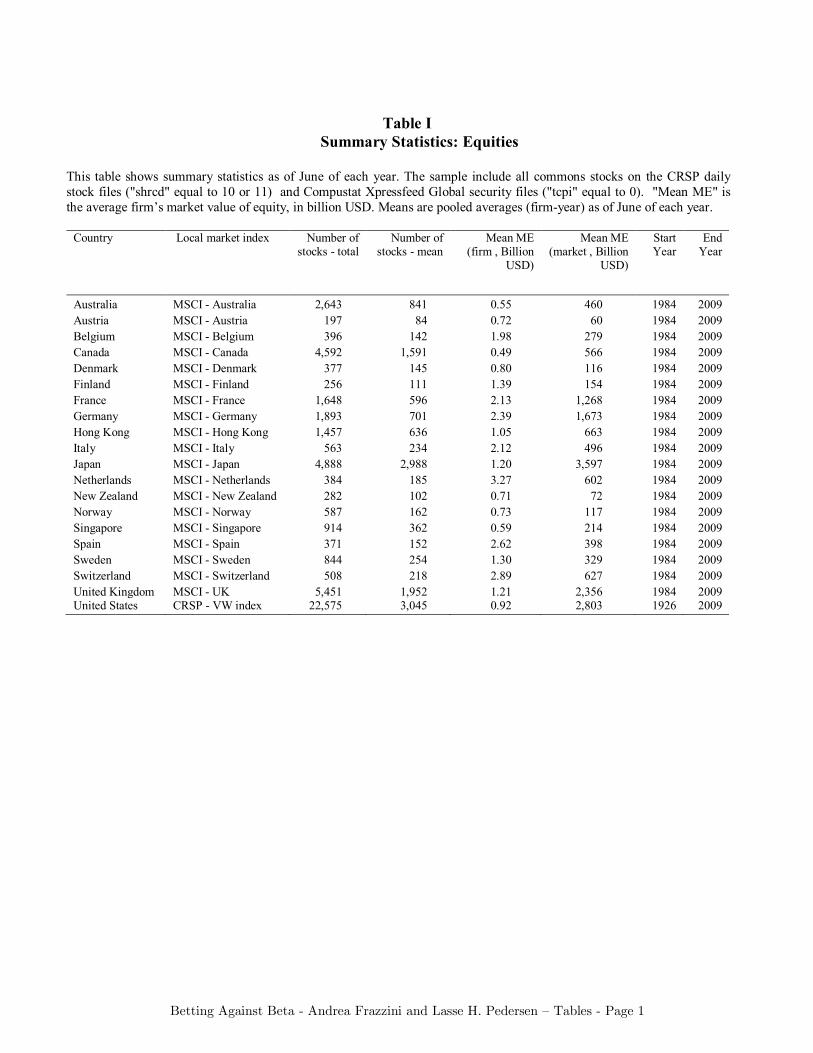
Betting Against Beta - Andrea Frazzini and Lasse H. Pedersen – Tables - Page 1
Table I
Summary Statistics: Equities
This table shows summary statistics as of June of each year. The sample include all commons stocks on the CRSP daily stock files ("shrcd" equal to 10 or 11) and Compustat Xpressfeed Global security files ("tcpi" equal to 0). "Mean ME" is the average firm’s market value of equity, in billion USD. Means are pooled averages (firm-year) as of June of each year. Country Local market index Number of
stocks - total Number of
stocks - mean Mean ME
(firm , Billion USD)
Mean ME (market , Billion
USD)
Start Year
End Year
Australia MSCI - Australia 2,643 841 0.55 460 1984 2009 Austria MSCI - Austria 197 84 0.72 60 1984 2009 Belgium MSCI - Belgium 396 142 1.98 279 1984 2009 Canada MSCI - Canada 4,592 1,591 0.49 566 1984 2009 Denmark MSCI - Denmark 377 145 0.80 116 1984 2009 Finland MSCI - Finland 256 111 1.39 154 1984 2009 France MSCI - France 1,648 596 2.13 1,268 1984 2009 Germany MSCI - Germany 1,893 701 2.39 1,673 1984 2009 Hong Kong MSCI - Hong Kong 1,457 636 1.05 663 1984 2009 Italy MSCI - Italy 563 234 2.12 496 1984 2009 Japan MSCI - Japan 4,888 2,988 1.20 3,597 1984 2009 Netherlands MSCI - Netherlands 384 185 3.27 602 1984 2009 New Zealand MSCI - New Zealand 282 102 0.71 72 1984 2009 Norway MSCI - Norway 587 162 0.73 117 1984 2009 Singapore MSCI - Singapore 914 362 0.59 214 1984 2009 Spain MSCI - Spain 371 152 2.62 398 1984 2009 Sweden MSCI - Sweden 844 254 1.30 329 1984 2009 Switzerland MSCI - Switzerland 508 218 2.89 627 1984 2009 United Kingdom MSCI - UK 5,451 1,952 1.21 2,356 1984 2009 United States CRSP - VW index 22,575 3,045 0.92 2,803 1926 2009
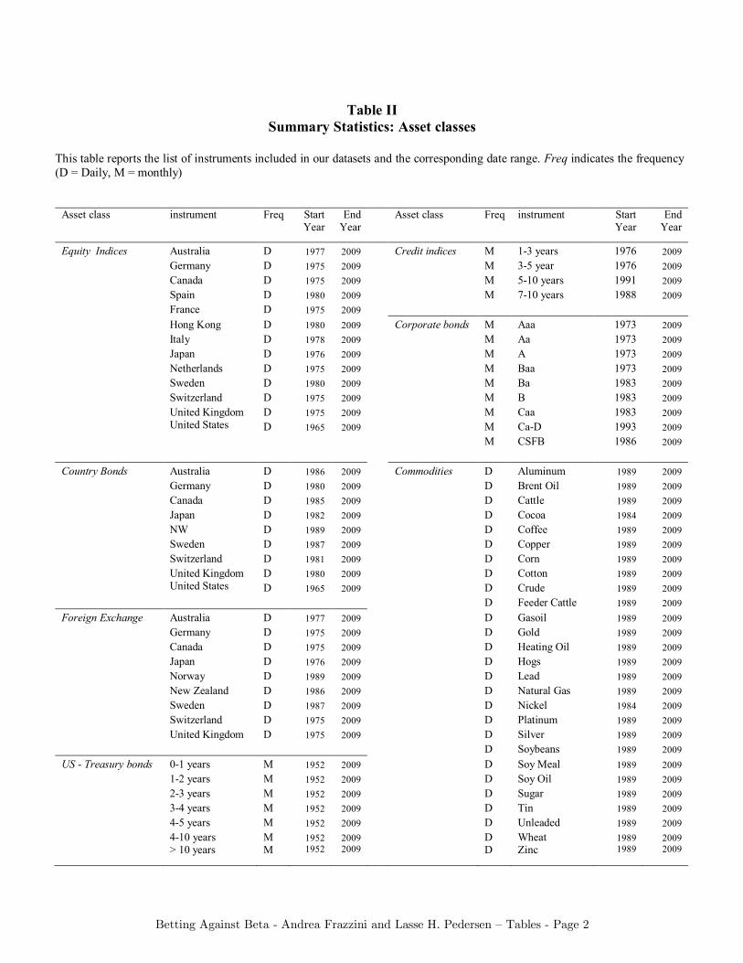
Betting Against Beta - Andrea Frazzini and Lasse H. Pedersen – Tables - Page 2
Table II
Summary Statistics: Asset classes
This table reports the list of instruments included in our datasets and the corresponding date range. Freq indicates the frequency (D = Daily, M = monthly)
Asset class instrument Freq Start Year
End Year
Asset class Freq instrument Start Year
End Year
Equity Indices Australia D 1977 2009 Credit indices M 1-3 years 1976 2009 Germany D 1975 2009 M 3-5 year 1976 2009 Canada D 1975 2009 M 5-10 years 1991 2009 Spain D 1980 2009 M 7-10 years 1988 2009 France D 1975 2009 Hong Kong D 1980 2009 Corporate bonds M Aaa 1973 2009 Italy D 1978 2009 M Aa 1973 2009 Japan D 1976 2009 M A 1973 2009 Netherlands D 1975 2009 M Baa 1973 2009 Sweden D 1980 2009 M Ba 1983 2009 Switzerland D 1975 2009 M B 1983 2009 United Kingdom D 1975 2009 M Caa 1983 2009 United States D 1965 2009 M Ca-D 1993 2009 M CSFB 1986 2009 Country Bonds Australia D 1986 2009 Commodities D Aluminum 1989 2009 Germany D 1980 2009 D Brent Oil 1989 2009 Canada D 1985 2009 D Cattle 1989 2009 Japan D 1982 2009 D Cocoa 1984 2009 NW D 1989 2009 D Coffee 1989 2009 Sweden D 1987 2009 D Copper 1989 2009 Switzerland D 1981 2009 D Corn 1989 2009 United Kingdom D 1980 2009 D Cotton 1989 2009 United States D 1965 2009 D Crude 1989 2009 D Feeder Cattle 1989 2009 Foreign Exchange Australia D 1977 2009 D Gasoil 1989 2009 Germany D 1975 2009 D Gold 1989 2009 Canada D 1975 2009 D Heating Oil 1989 2009 Japan D 1976 2009 D Hogs 1989 2009 Norway D 1989 2009 D Lead 1989 2009 New Zealand D 1986 2009 D Natural Gas 1989 2009 Sweden D 1987 2009 D Nickel 1984 2009 Switzerland D 1975 2009 D Platinum 1989 2009 United Kingdom D 1975 2009 D Silver 1989 2009 D Soybeans 1989 2009 US - Treasury bonds 0-1 years M 1952 2009 D Soy Meal 1989 2009 1-2 years M 1952 2009 D Soy Oil 1989 2009 2-3 years M 1952 2009 D Sugar 1989 2009 3-4 years M 1952 2009 D Tin 1989 2009 4-5 years M 1952 2009 D Unleaded 1989 2009 4-10 years M 1952 2009 D Wheat 1989 2009
> 10 years M 1952 2009 D Zinc 1989 2009
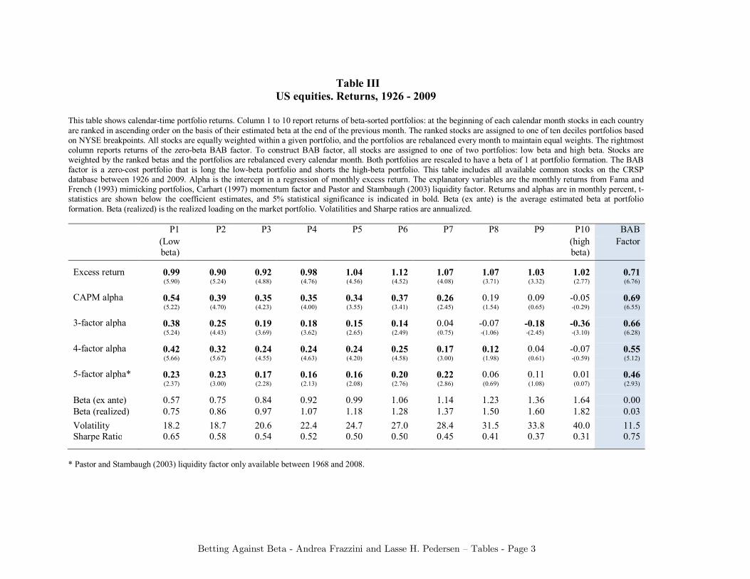
Betting Against Beta - Andrea Frazzini and Lasse H. Pedersen – Tables - Page 3
Table III US equities. Returns, 1926 - 2009
This table shows calendar-time portfolio returns. Column 1 to 10 report returns of beta-sorted portfolios: at the beginning of each calendar month stocks in each country are ranked in ascending order on the basis of their estimated beta at the end of the previous month. The ranked stocks are assigned to one of ten deciles portfolios based on NYSE breakpoints. All stocks are equally weighted within a given portfolio, and the portfolios are rebalanced every month to maintain equal weights. The rightmost column reports returns of the zero-beta BAB factor. To construct BAB factor, all stocks are assigned to one of two portfolios: low beta and high beta. Stocks are weighted by the ranked betas and the portfolios are rebalanced every calendar month. Both portfolios are rescaled to have a beta of 1 at portfolio formation. The BAB factor is a zero-cost portfolio that is long the low-beta portfolio and shorts the high-beta portfolio. This table includes all available common stocks on the CRSP database between 1926 and 2009. Alpha is the intercept in a regression of monthly excess return. The explanatory variables are the monthly returns from Fama and French (1993) mimicking portfolios, Carhart (1997) momentum factor and Pastor and Stambaugh (2003) liquidity factor. Returns and alphas are in monthly percent, t-statistics are shown below the coefficient estimates, and 5% statistical significance is indicated in bold. Beta (ex ante) is the average estimated beta at portfolio formation. Beta (realized) is the realized loading on the market portfolio. Volatilities and Sharpe ratios are annualized.
P1 P2 P3 P4 P5 P6 P7 P8 P9 P10 BAB
(Low beta)
(high beta)
Factor
Excess return 0.99 0.90 0.92 0.98 1.04 1.12 1.07 1.07 1.03 1.02 0.71 (5.90) (5.24) (4.88) (4.76) (4.56) (4.52) (4.08) (3.71) (3.32) (2.77) (6.76)
CAPM alpha 0.54 0.39 0.35 0.35 0.34 0.37 0.26 0.19 0.09 -0.05 0.69 (5.22) (4.70) (4.23) (4.00) (3.55) (3.41) (2.45) (1.54) (0.65) -(0.29) (6.55)
3-factor alpha 0.38 0.25 0.19 0.18 0.15 0.14 0.04 -0.07 -0.18 -0.36 0.66 (5.24) (4.43) (3.69) (3.62) (2.65) (2.49) (0.75) -(1.06) -(2.45) -(3.10) (6.28)
4-factor alpha 0.42 0.32 0.24 0.24 0.24 0.25 0.17 0.12 0.04 -0.07 0.55 (5.66) (5.67) (4.55) (4.63) (4.20) (4.58) (3.00) (1.98) (0.61) -(0.59) (5.12)
5-factor alpha* 0.23 0.23 0.17 0.16 0.16 0.20 0.22 0.06 0.11 0.01 0.46 (2.37) (3.00) (2.28) (2.13) (2.08) (2.76) (2.86) (0.69) (1.08) (0.07) (2.93)
Beta (ex ante) 0.57 0.75 0.84 0.92 0.99 1.06 1.14 1.23 1.36 1.64 0.00 Beta (realized) 0.75 0.86 0.97 1.07 1.18 1.28 1.37 1.50 1.60 1.82 0.03 Volatility 18.2 18.7 20.6 22.4 24.7 27.0 28.4 31.5 33.8 40.0 11.5 Sharpe Ratio 0.65 0.58 0.54 0.52 0.50 0.50 0.45 0.41 0.37 0.31 0.75
* Pastor and Stambaugh (2003) liquidity factor only available between 1968 and 2008.
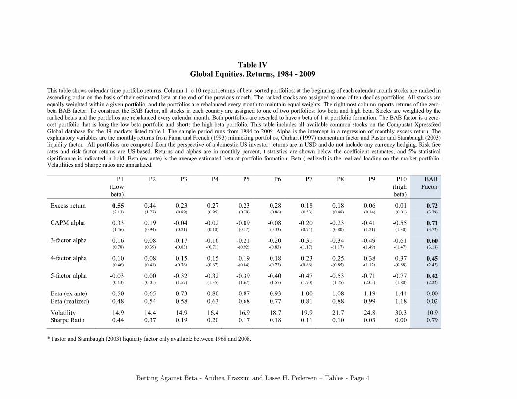
Betting Against Beta - Andrea Frazzini and Lasse H. Pedersen – Tables - Page 4
Table IV
Global Equities. Returns, 1984 - 2009
This table shows calendar-time portfolio returns. Column 1 to 10 report returns of beta-sorted portfolios: at the beginning of each calendar month stocks are ranked in ascending order on the basis of their estimated beta at the end of the previous month. The ranked stocks are assigned to one of ten deciles portfolios. All stocks are equally weighted within a given portfolio, and the portfolios are rebalanced every month to maintain equal weights. The rightmost column reports returns of the zero-beta BAB factor. To construct the BAB factor, all stocks in each country are assigned to one of two portfolios: low beta and high beta. Stocks are weighted by the ranked betas and the portfolios are rebalanced every calendar month. Both portfolios are rescaled to have a beta of 1 at portfolio formation. The BAB factor is a zero-cost portfolio that is long the low-beta portfolio and shorts the high-beta portfolio. This table includes all available common stocks on the Compustat Xpressfeed Global database for the 19 markets listed table I. The sample period runs from 1984 to 2009. Alpha is the intercept in a regression of monthly excess return. The explanatory variables are the monthly returns from Fama and French (1993) mimicking portfolios, Carhart (1997) momentum factor and Pastor and Stambaugh (2003) liquidity factor. All portfolios are computed from the perspective of a domestic US investor: returns are in USD and do not include any currency hedging. Risk free rates and risk factor returns are US-based. Returns and alphas are in monthly percent, t-statistics are shown below the coefficient estimates, and 5% statistical significance is indicated in bold. Beta (ex ante) is the average estimated beta at portfolio formation. Beta (realized) is the realized loading on the market portfolio. Volatilities and Sharpe ratios are annualized.
P1 P2 P3 P4 P5 P6 P7 P8 P9 P10 BAB
(Low beta)
(high beta)
Factor
Excess return 0.55 0.44 0.23 0.27 0.23 0.28 0.18 0.18 0.06 0.01 0.72 (2.13) (1.77) (0.89) (0.95) (0.79) (0.86) (0.53) (0.48) (0.14) (0.01) (3.79)
CAPM alpha 0.33 0.19 -0.04 -0.02 -0.09 -0.08 -0.20 -0.23 -0.41 -0.55 0.71 (1.46) (0.94) -(0.21) -(0.10) -(0.37) -(0.33) -(0.74) -(0.80) -(1.21) -(1.30) (3.72)
3-factor alpha 0.16 0.08 -0.17 -0.16 -0.21 -0.20 -0.31 -0.34 -0.49 -0.61 0.60 (0.78) (0.39) -(0.83) -(0.71) -(0.92) -(0.83) -(1.17) -(1.17) -(1.49) -(1.47) (3.18)
4-factor alpha 0.10 0.08 -0.15 -0.15 -0.19 -0.18 -0.23 -0.25 -0.38 -0.37 0.45 (0.46) (0.41) -(0.76) -(0.67) -(0.84) -(0.73) -(0.86) -(0.85) -(1.12) -(0.88) (2.47)
5-factor alpha -0.03 0.00 -0.32 -0.32 -0.39 -0.40 -0.47 -0.53 -0.71 -0.77 0.42 -(0.13) -(0.01) -(1.57) -(1.35) -(1.67) -(1.57) -(1.70) -(1.75) -(2.05) -(1.80) (2.22)
Beta (ex ante) 0.50 0.65 0.73 0.80 0.87 0.93 1.00 1.08 1.19 1.44 0.00 Beta (realized) 0.48 0.54 0.58 0.63 0.68 0.77 0.81 0.88 0.99 1.18 0.02
Volatility 14.9 14.4 14.9 16.4 16.9 18.7 19.9 21.7 24.8 30.3 10.9 Sharpe Ratio 0.44 0.37 0.19 0.20 0.17 0.18 0.11 0.10 0.03 0.00 0.79
* Pastor and Stambaugh (2003) liquidity factor only available between 1968 and 2008.
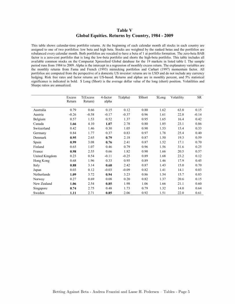
Betting Against Beta - Andrea Frazzini and Lasse H. Pedersen – Tables - Page 5
Table V Global Equities. Returns by Country, 1984 - 2009
This table shows calendar-time portfolio returns. At the beginning of each calendar month all stocks in each country are assigned to one of two portfolios: low beta and high beta. Stocks are weighted by the ranked betas and the portfolios are rebalanced every calendar month. Both portfolios are rescaled to have a beta of 1 at portfolio formation. The zero-beta BAB factor is a zero-cost portfolio that is long the low-beta portfolio and shorts the high-beta portfolio. This table includes all available common stocks on the Compustat Xpressfeed Global database for the 19 markets in listed table I. The sample period runs from 1984 to 2009. Alpha is the intercept in a regression of monthly excess return. The explanatory variables are the monthly returns from Fama and French (1993) mimicking portfolios and Carhart (1997) momentum factor. All portfolios are computed from the perspective of a domestic US investor: returns are in USD and do not include any currency hedging. Risk free rates and factor returns are US-based. Returns and alphas are in monthly percent, and 5% statistical significance is indicated in bold. $ Long (Short) is the average dollar value of the long (short) position. Volatilities and Sharpe ratios are annualized.
Excess Return
T(Excess Return)
4-factor alpha
T(alpha) $Short $Long Volatility SR
Australia 0.79 0.66 0.15 0.12 0.80 1.62 63.8 0.15 Austria -0.26 -0.58 -0.17 -0.37 0.96 1.61 22.8 -0.14 Belgium 0.57 1.53 0.52 1.37 0.95 1.65 16.4 0.42 Canada 1.66 4.10 1.07 2.78 0.80 1.85 23.1 0.86 Switzerland 0.42 1.46 0.30 1.05 0.90 1.53 15.4 0.33 Germany 0.84 1.77 0.37 0.83 0.97 1.78 25.4 0.40 Denmark 0.95 2.65 0.79 2.18 0.87 1.50 19.3 0.59 Spain 0.99 3.08 0.76 2.41 0.87 1.52 17.1 0.70 Finland 0.65 1.07 0.46 0.79 0.96 1.56 31.6 0.25 France 0.98 2.55 0.66 1.82 0.90 1.66 20.5 0.57 United Kingdom 0.23 0.54 -0.11 -0.25 0.89 1.68 23.2 0.12 Hong Kong 0.68 1.96 0.33 0.95 0.89 1.46 17.9 0.45 Italy 0.88 3.14 0.68 2.42 0.87 1.43 15.0 0.70 Japan 0.03 0.12 -0.03 -0.09 0.82 1.41 14.1 0.03 Netherlands 1.09 3.72 0.94 3.23 0.86 1.54 15.7 0.83 Norway 0.27 0.69 0.08 0.20 0.82 1.37 20.6 0.15 New Zealand 1.06 2.54 0.85 1.98 1.06 1.66 21.1 0.60 Singapore 0.74 2.75 0.48 1.73 0.79 1.32 14.0 0.64 Sweden 1.11 2.71 0.85 2.06 0.92 1.51 22.0 0.61
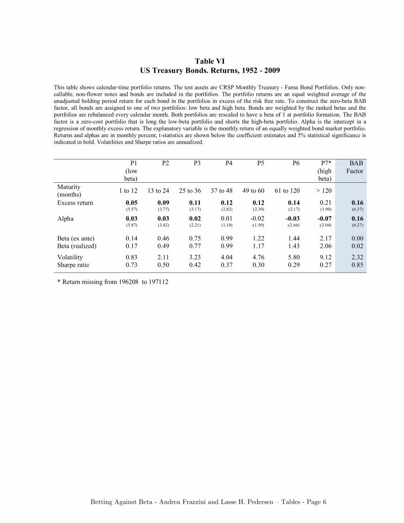
Betting Against Beta - Andrea Frazzini and Lasse H. Pedersen – Tables - Page 6
Table VI
US Treasury Bonds. Returns, 1952 - 2009 This table shows calendar-time portfolio returns. The test assets are CRSP Monthly Treasury - Fama Bond Portfolios. Only non-callable, non-flower notes and bonds are included in the portfolios. The portfolio returns are an equal weighted average of the unadjusted holding period return for each bond in the portfolios in excess of the risk free rate. To construct the zero-beta BAB factor, all bonds are assigned to one of two portfolios: low beta and high beta. Bonds are weighted by the ranked betas and the portfolios are rebalanced every calendar month. Both portfolios are rescaled to have a beta of 1 at portfolio formation. The BAB factor is a zero-cost portfolio that is long the low-beta portfolio and shorts the high-beta portfolio. Alpha is the intercept in a regression of monthly excess return. The explanatory variable is the monthly return of an equally weighted bond market portfolio. Returns and alphas are in monthly percent, t-statistics are shown below the coefficient estimates and 5% statistical significance is indicated in bold. Volatilities and Sharpe ratios are annualized.
P1 P2 P3 P4 P5 P6 P7* BAB (low
beta) (high
beta) Factor
Maturity (months) 1 to 12 13 to 24 25 to 36 37 to 48 49 to 60 61 to 120 > 120
Excess return 0.05 0.09 0.11 0.12 0.12 0.14 0.21 0.16 (5.57) (3.77) (3.17) (2.82) (2.30) (2.17) (1.90) (6.37)
Alpha 0.03 0.03 0.02 0.01 -0.02 -0.03 -0.07 0.16 (5.87) (3.42) (2.21) (1.10) -(1.59) -(2.66) -(2.04) (6.27)
Beta (ex ante) 0.14 0.46 0.75 0.99 1.22 1.44 2.17 0.00 Beta (realized) 0.17 0.49 0.77 0.99 1.17 1.43 2.06 0.02
Volatility 0.83 2.11 3.23 4.04 4.76 5.80 9.12 2.32 Sharpe ratio 0.73 0.50 0.42 0.37 0.30 0.29 0.27 0.85
* Return missing from 196208 to 197112
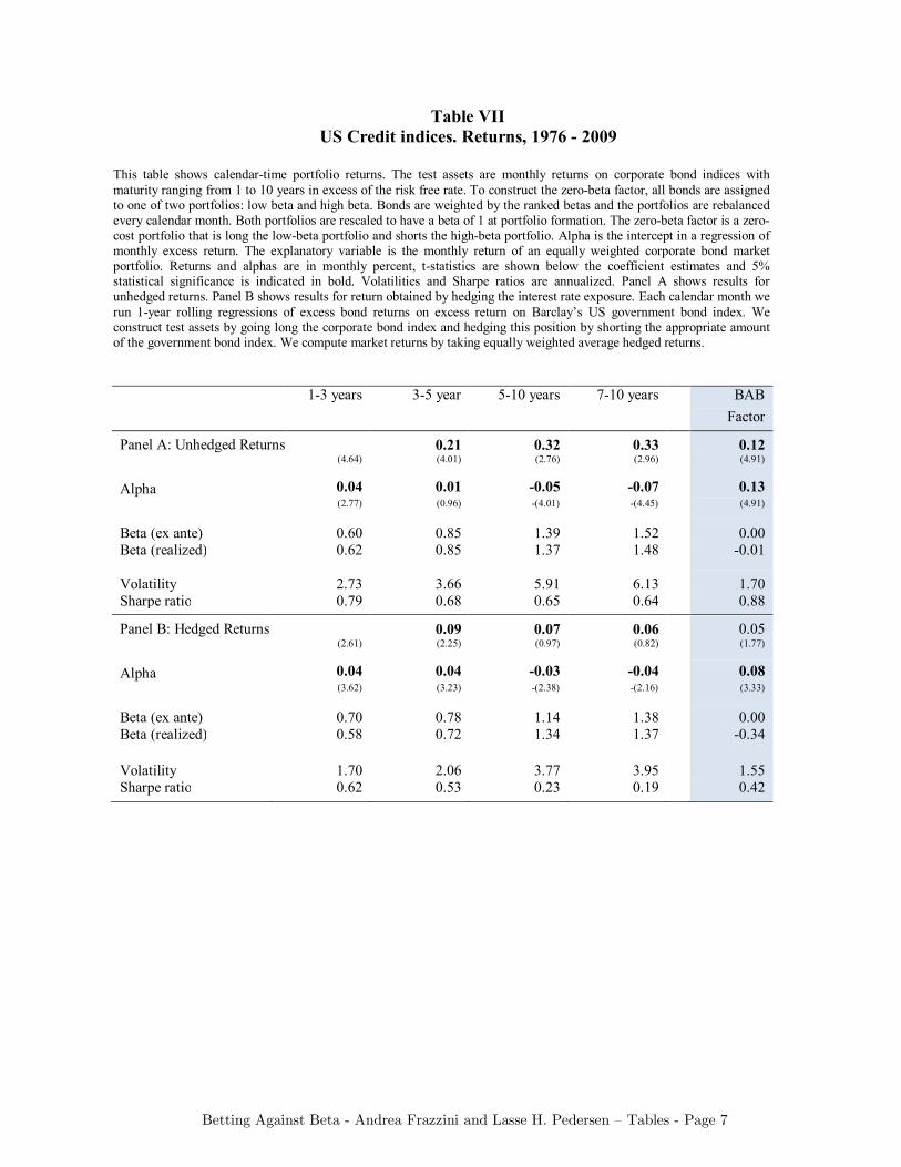
Betting Against Beta - Andrea Frazzini and Lasse H. Pedersen – Tables - Page 7
Table VII US Credit indices. Returns, 1976 - 2009
This table shows calendar-time portfolio returns. The test assets are monthly returns on corporate bond indices with maturity ranging from 1 to 10 years in excess of the risk free rate. To construct the zero-beta factor, all bonds are assigned to one of two portfolios: low beta and high beta. Bonds are weighted by the ranked betas and the portfolios are rebalanced every calendar month. Both portfolios are rescaled to have a beta of 1 at portfolio formation. The zero-beta factor is a zero-cost portfolio that is long the low-beta portfolio and shorts the high-beta portfolio. Alpha is the intercept in a regression of monthly excess return. The explanatory variable is the monthly return of an equally weighted corporate bond market portfolio. Returns and alphas are in monthly percent, t-statistics are shown below the coefficient estimates and 5% statistical significance is indicated in bold. Volatilities and Sharpe ratios are annualized. Panel A shows results for unhedged returns. Panel B shows results for return obtained by hedging the interest rate exposure. Each calendar month we run 1-year rolling regressions of excess bond returns on excess return on Barclay’s US government bond index. We construct test assets by going long the corporate bond index and hedging this position by shorting the appropriate amount of the government bond index. We compute market returns by taking equally weighted average hedged returns.
1-3 years 3-5 year 5-10 years 7-10 years BAB Factor
Panel A: Unhedged Returns 0.21 0.32 0.33 0.12 (4.64) (4.01) (2.76) (2.96) (4.91)
Alpha 0.04 0.01 -0.05 -0.07 0.13 (2.77) (0.96) -(4.01) -(4.45) (4.91)
Beta (ex ante) 0.60 0.85 1.39 1.52 0.00 Beta (realized) 0.62 0.85 1.37 1.48 -0.01
Volatility 2.73 3.66 5.91 6.13 1.70 Sharpe ratio 0.79 0.68 0.65 0.64 0.88
Panel B: Hedged Returns 0.09 0.07 0.06 0.05 (2.61) (2.25) (0.97) (0.82) (1.77)
Alpha 0.04 0.04 -0.03 -0.04 0.08 (3.62) (3.23) -(2.38) -(2.16) (3.33)
Beta (ex ante) 0.70 0.78 1.14 1.38 0.00 Beta (realized) 0.58 0.72 1.34 1.37 -0.34
Volatility 1.70 2.06 3.77 3.95 1.55 Sharpe ratio 0.62 0.53 0.23 0.19 0.42
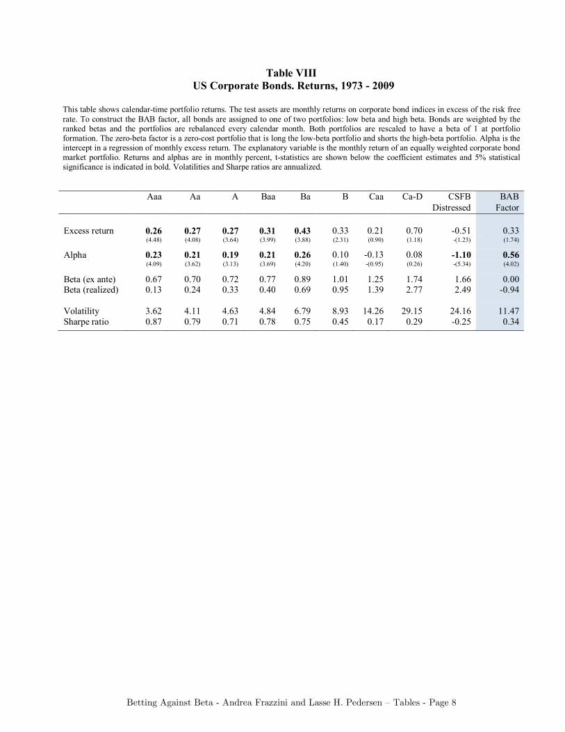
Betting Against Beta - Andrea Frazzini and Lasse H. Pedersen – Tables - Page 8
Table VIII US Corporate Bonds. Returns, 1973 - 2009
This table shows calendar-time portfolio returns. The test assets are monthly returns on corporate bond indices in excess of the risk free rate. To construct the BAB factor, all bonds are assigned to one of two portfolios: low beta and high beta. Bonds are weighted by the ranked betas and the portfolios are rebalanced every calendar month. Both portfolios are rescaled to have a beta of 1 at portfolio formation. The zero-beta factor is a zero-cost portfolio that is long the low-beta portfolio and shorts the high-beta portfolio. Alpha is the intercept in a regression of monthly excess return. The explanatory variable is the monthly return of an equally weighted corporate bond market portfolio. Returns and alphas are in monthly percent, t-statistics are shown below the coefficient estimates and 5% statistical significance is indicated in bold. Volatilities and Sharpe ratios are annualized.
Aaa Aa A Baa Ba B Caa Ca-D CSFB BAB Distressed Factor
Excess return 0.26 0.27 0.27 0.31 0.43 0.33 0.21 0.70 -0.51 0.33 (4.48) (4.08) (3.64) (3.99) (3.88) (2.31) (0.90) (1.18) -(1.23) (1.74)
Alpha 0.23 0.21 0.19 0.21 0.26 0.10 -0.13 0.08 -1.10 0.56 (4.09) (3.62) (3.13) (3.69) (4.20) (1.40) -(0.95) (0.26) -(5.34) (4.02)
Beta (ex ante) 0.67 0.70 0.72 0.77 0.89 1.01 1.25 1.74 1.66 0.00 Beta (realized) 0.13 0.24 0.33 0.40 0.69 0.95 1.39 2.77 2.49 -0.94
Volatility 3.62 4.11 4.63 4.84 6.79 8.93 14.26 29.15 24.16 11.47 Sharpe ratio 0.87 0.79 0.71 0.78 0.75 0.45 0.17 0.29 -0.25 0.34
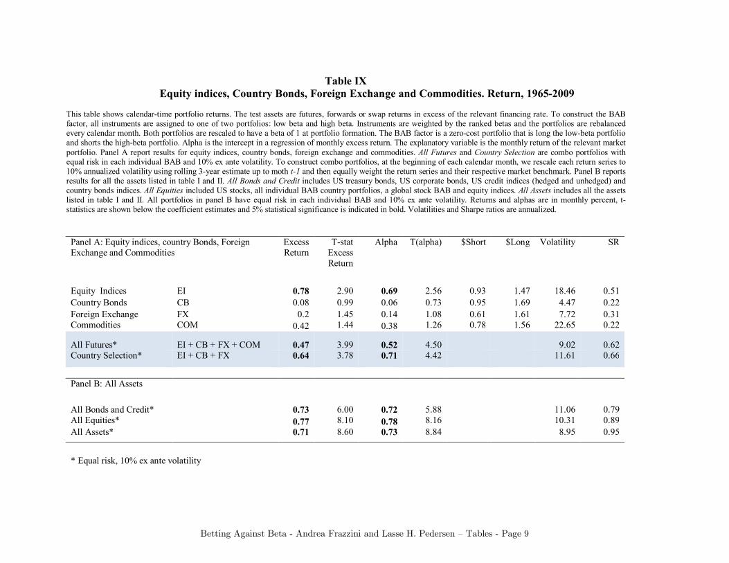
Betting Against Beta - Andrea Frazzini and Lasse H. Pedersen – Tables - Page 9
Table IX Equity indices, Country Bonds, Foreign Exchange and Commodities. Return, 1965-2009
This table shows calendar-time portfolio returns. The test assets are futures, forwards or swap returns in excess of the relevant financing rate. To construct the BAB factor, all instruments are assigned to one of two portfolios: low beta and high beta. Instruments are weighted by the ranked betas and the portfolios are rebalanced every calendar month. Both portfolios are rescaled to have a beta of 1 at portfolio formation. The BAB factor is a zero-cost portfolio that is long the low-beta portfolio and shorts the high-beta portfolio. Alpha is the intercept in a regression of monthly excess return. The explanatory variable is the monthly return of the relevant market portfolio. Panel A report results for equity indices, country bonds, foreign exchange and commodities. All Futures and Country Selection are combo portfolios with equal risk in each individual BAB and 10% ex ante volatility. To construct combo portfolios, at the beginning of each calendar month, we rescale each return series to 10% annualized volatility using rolling 3-year estimate up to moth t-1 and then equally weight the return series and their respective market benchmark. Panel B reports results for all the assets listed in table I and II. All Bonds and Credit includes US treasury bonds, US corporate bonds, US credit indices (hedged and unhedged) and country bonds indices. All Equities included US stocks, all individual BAB country portfolios, a global stock BAB and equity indices. All Assets includes all the assets listed in table I and II. All portfolios in panel B have equal risk in each individual BAB and 10% ex ante volatility. Returns and alphas are in monthly percent, t-statistics are shown below the coefficient estimates and 5% statistical significance is indicated in bold. Volatilities and Sharpe ratios are annualized.
Panel A: Equity indices, country Bonds, Foreign Exchange and Commodities
Excess Return
T-stat Excess Return
Alpha T(alpha) $Short $Long Volatility SR
Equity Indices EI 0.78 2.90 0.69 2.56 0.93 1.47 18.46 0.51 Country Bonds CB 0.08 0.99 0.06 0.73 0.95 1.69 4.47 0.22 Foreign Exchange FX 0.2 1.45 0.14 1.08 0.61 1.61 7.72 0.31 Commodities COM 0.42 1.44 0.38 1.26 0.78 1.56 22.65 0.22
All Futures* EI + CB + FX + COM 0.47 3.99 0.52 4.50 9.02 0.62 Country Selection* EI + CB + FX 0.64 3.78 0.71 4.42 11.61 0.66
Panel B: All Assets
All Bonds and Credit* 0.73 6.00 0.72 5.88 11.06 0.79 All Equities* 0.77 8.10 0.78 8.16 10.31 0.89 All Assets* 0.71 8.60 0.73 8.84 8.95 0.95
* Equal risk, 10% ex ante volatility
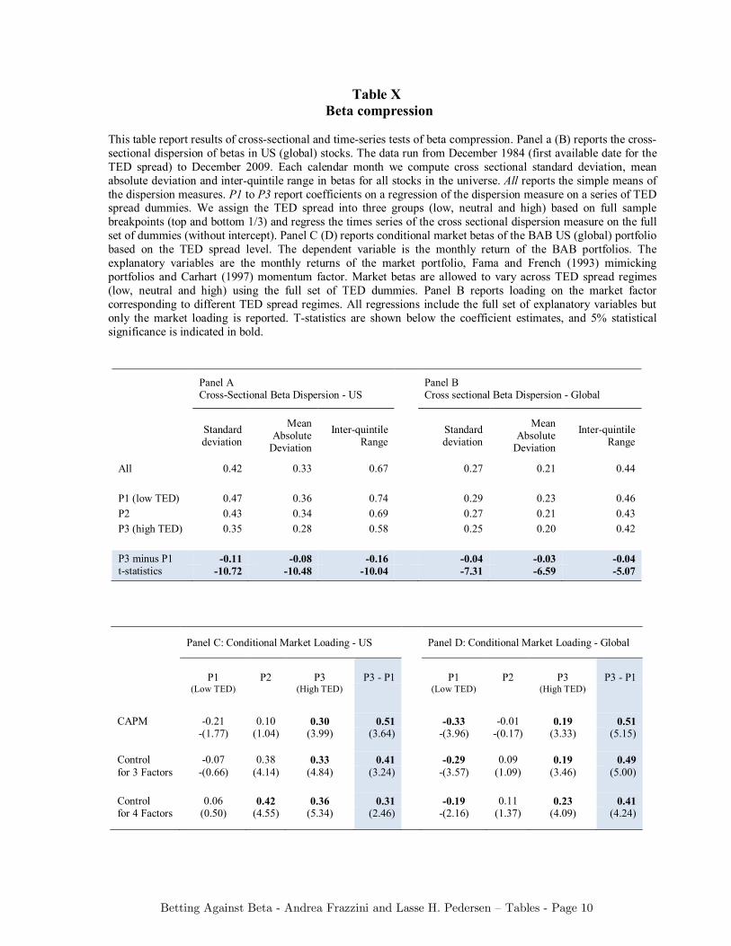
Betting Against Beta - Andrea Frazzini and Lasse H. Pedersen – Tables - Page 10
Table X Beta compression
This table report results of cross-sectional and time-series tests of beta compression. Panel a (B) reports the cross-sectional dispersion of betas in US (global) stocks. The data run from December 1984 (first available date for the TED spread) to December 2009. Each calendar month we compute cross sectional standard deviation, mean absolute deviation and inter-quintile range in betas for all stocks in the universe. All reports the simple means of the dispersion measures. P1 to P3 report coefficients on a regression of the dispersion measure on a series of TED spread dummies. We assign the TED spread into three groups (low, neutral and high) based on full sample breakpoints (top and bottom 1/3) and regress the times series of the cross sectional dispersion measure on the full set of dummies (without intercept). Panel C (D) reports conditional market betas of the BAB US (global) portfolio based on the TED spread level. The dependent variable is the monthly return of the BAB portfolios. The explanatory variables are the monthly returns of the market portfolio, Fama and French (1993) mimicking portfolios and Carhart (1997) momentum factor. Market betas are allowed to vary across TED spread regimes (low, neutral and high) using the full set of TED dummies. Panel B reports loading on the market factor corresponding to different TED spread regimes. All regressions include the full set of explanatory variables but only the market loading is reported. T-statistics are shown below the coefficient estimates, and 5% statistical significance is indicated in bold.
Panel A
Cross-Sectional Beta Dispersion - US Panel B Cross sectional Beta Dispersion - Global
Standard deviation
Mean Absolute
Deviation
Inter-quintile Range Standard
deviation
Mean Absolute
Deviation
Inter-quintile Range
All 0.42 0.33 0.67 0.27 0.21 0.44
P1 (low TED) 0.47 0.36 0.74 0.29 0.23 0.46 P2 0.43 0.34 0.69 0.27 0.21 0.43 P3 (high TED) 0.35 0.28 0.58 0.25 0.20 0.42
P3 minus P1 -0.11 -0.08 -0.16 -0.04 -0.03 -0.04 t-statistics -10.72 -10.48 -10.04 -7.31 -6.59 -5.07
Panel C: Conditional Market Loading - US Panel D: Conditional Market Loading - Global
P1 P2 P3 P3 - P1 P1 P2 P3 P3 - P1 (Low TED) (High TED) (Low TED) (High TED)
CAPM -0.21 0.10 0.30 0.51 -0.33 -0.01 0.19 0.51
-(1.77) (1.04) (3.99) (3.64) -(3.96) -(0.17) (3.33) (5.15)
Control -0.07 0.38 0.33 0.41 -0.29 0.09 0.19 0.49 for 3 Factors -(0.66) (4.14) (4.84) (3.24) -(3.57) (1.09) (3.46) (5.00)
Control 0.06 0.42 0.36 0.31 -0.19 0.11 0.23 0.41 for 4 Factors (0.50) (4.55) (5.34) (2.46) -(2.16) (1.37) (4.09) (4.24)
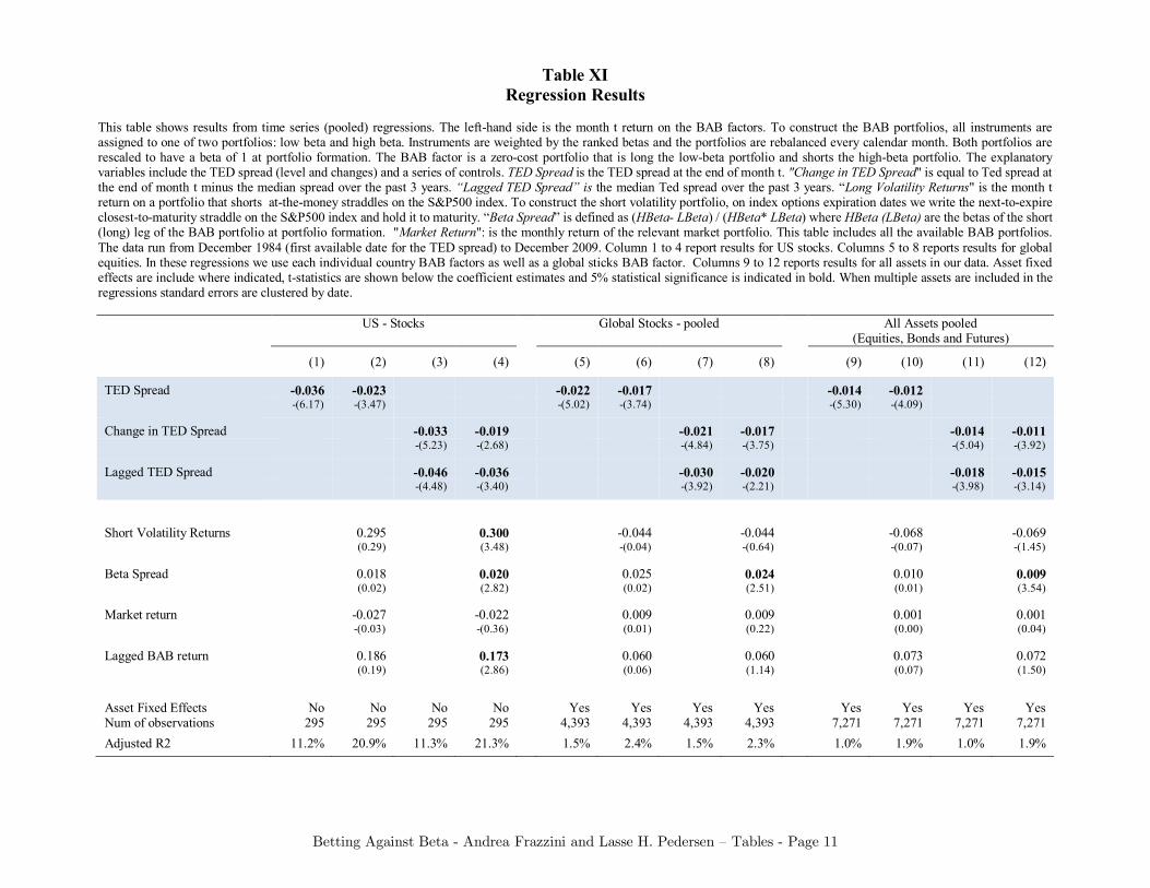
Betting Against Beta - Andrea Frazzini and Lasse H. Pedersen – Tables - Page 11
Table XI Regression Results
This table shows results from time series (pooled) regressions. The left-hand side is the month t return on the BAB factors. To construct the BAB portfolios, all instruments are assigned to one of two portfolios: low beta and high beta. Instruments are weighted by the ranked betas and the portfolios are rebalanced every calendar month. Both portfolios are rescaled to have a beta of 1 at portfolio formation. The BAB factor is a zero-cost portfolio that is long the low-beta portfolio and shorts the high-beta portfolio. The explanatory variables include the TED spread (level and changes) and a series of controls. TED Spread is the TED spread at the end of month t. "Change in TED Spread" is equal to Ted spread at the end of month t minus the median spread over the past 3 years. “Lagged TED Spread” is the median Ted spread over the past 3 years. “Long Volatility Returns" is the month t return on a portfolio that shorts at-the-money straddles on the S&P500 index. To construct the short volatility portfolio, on index options expiration dates we write the next-to-expire closest-to-maturity straddle on the S&P500 index and hold it to maturity. “Beta Spread” is defined as (HBeta- LBeta) / (HBeta* LBeta) where HBeta (LBeta) are the betas of the short (long) leg of the BAB portfolio at portfolio formation. "Market Return": is the monthly return of the relevant market portfolio. This table includes all the available BAB portfolios. The data run from December 1984 (first available date for the TED spread) to December 2009. Column 1 to 4 report results for US stocks. Columns 5 to 8 reports results for global equities. In these regressions we use each individual country BAB factors as well as a global sticks BAB factor. Columns 9 to 12 reports results for all assets in our data. Asset fixed effects are include where indicated, t-statistics are shown below the coefficient estimates and 5% statistical significance is indicated in bold. When multiple assets are included in the regressions standard errors are clustered by date. US - Stocks Global Stocks - pooled All Assets pooled
(Equities, Bonds and Futures)
(1) (2) (3) (4) (5) (6) (7) (8) (9) (10) (11) (12)
TED Spread -0.036 -0.023 -0.022 -0.017 -0.014 -0.012 -(6.17) -(3.47) -(5.02) -(3.74) -(5.30) -(4.09)
Change in TED Spread -0.033 -0.019 -0.021 -0.017 -0.014 -0.011 -(5.23) -(2.68) -(4.84) -(3.75) -(5.04) -(3.92)
Lagged TED Spread -0.046 -0.036 -0.030 -0.020 -0.018 -0.015 -(4.48) -(3.40) -(3.92) -(2.21) -(3.98) -(3.14)
Short Volatility Returns 0.295 0.300 -0.044 -0.044 -0.068 -0.069 (0.29) (3.48) -(0.04) -(0.64) -(0.07) -(1.45)
Beta Spread 0.018 0.020 0.025 0.024 0.010 0.009 (0.02) (2.82) (0.02) (2.51) (0.01) (3.54)
Market return -0.027 -0.022 0.009 0.009 0.001 0.001 -(0.03) -(0.36) (0.01) (0.22) (0.00) (0.04)
Lagged BAB return 0.186 0.173 0.060 0.060 0.073 0.072 (0.19) (2.86) (0.06) (1.14) (0.07) (1.50)
Asset Fixed Effects No No No No Yes Yes Yes Yes Yes Yes Yes Yes Num of observations 295 295 295 295 4,393 4,393 4,393 4,393 7,271 7,271 7,271 7,271 Adjusted R2 11.2% 20.9% 11.3% 21.3% 1.5% 2.4% 1.5% 2.3% 1.0% 1.9% 1.0% 1.9%
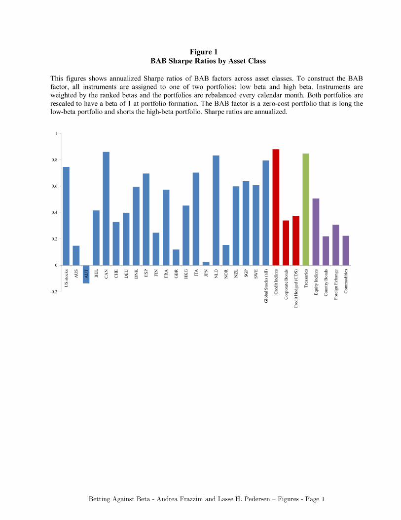
Betting Against Beta - Andrea Frazzini and Lasse H. Pedersen – Figures - Page 1
Figure 1 BAB Sharpe Ratios by Asset Class
This figures shows annualized Sharpe ratios of BAB factors across asset classes. To construct the BAB factor, all instruments are assigned to one of two portfolios: low beta and high beta. Instruments are weighted by the ranked betas and the portfolios are rebalanced every calendar month. Both portfolios are rescaled to have a beta of 1 at portfolio formation. The BAB factor is a zero-cost portfolio that is long the low-beta portfolio and shorts the high-beta portfolio. Sharpe ratios are annualized.
-0.2
0
0.2
0.4
0.6
0.8
1
US
stoc
ks
AU
S
AU
T
BEL
CA
N
CH
E
DEU
DN
K
ESP
FIN
FRA
GB
R
HK
G
ITA
JPN
NLD
NO
R
NZL SG
P
SWE
Glo
bal S
tock
s (al
l)
Cre
dit I
ndic
es
Cor
pora
te B
onds
Cre
dit H
edge
d (C
DS)
Trea
surie
s
Equi
ty In
dice
s
Cou
ntry
Bon
ds
Fore
ign
Echa
nge
Com
mod
ities
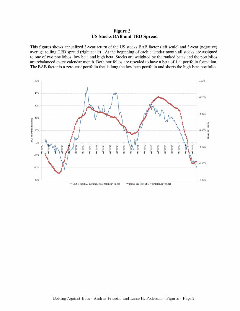
Betting Against Beta - Andrea Frazzini and Lasse H. Pedersen – Figures - Page 2
Figure 2 US Stocks BAB and TED Spread
This figures shows annualized 3-year return of the US stocks BAB factor (left scale) and 3-year (negative) average rolling TED spread (right scale) . At the beginning of each calendar month all stocks are assigned to one of two portfolios: low beta and high beta. Stocks are weighted by the ranked betas and the portfolios are rebalanced every calendar month. Both portfolios are rescaled to have a beta of 1 at portfolio formation. The BAB factor is a zero-cost portfolio that is long the low-beta portfolio and shorts the high-beta portfolio.
-1.20%
-1.00%
-0.80%
-0.60%
-0.40%
-0.20%
0.00%
-30%
-20%
-10%
0%
10%
20%
30%
40%
50%
05/0
1/87
05/0
1/88
05/0
1/89
05/0
1/90
05/0
1/91
05/0
1/92
05/0
1/93
05/0
1/94
05/0
1/95
05/0
1/96
05/0
1/97
05/0
1/98
05/0
1/99
05/0
1/00
05/0
1/01
05/0
1/02
05/0
1/03
05/0
1/04
05/0
1/05
05/0
1/06
05/0
1/07
05/0
1/08
05/0
1/09
Minus Ted spread
BAB
retu
rn (a
nnua
lized
)
US Stocks BAB Return (3-year rolling average) minus Ted spread (3-year rolling average)
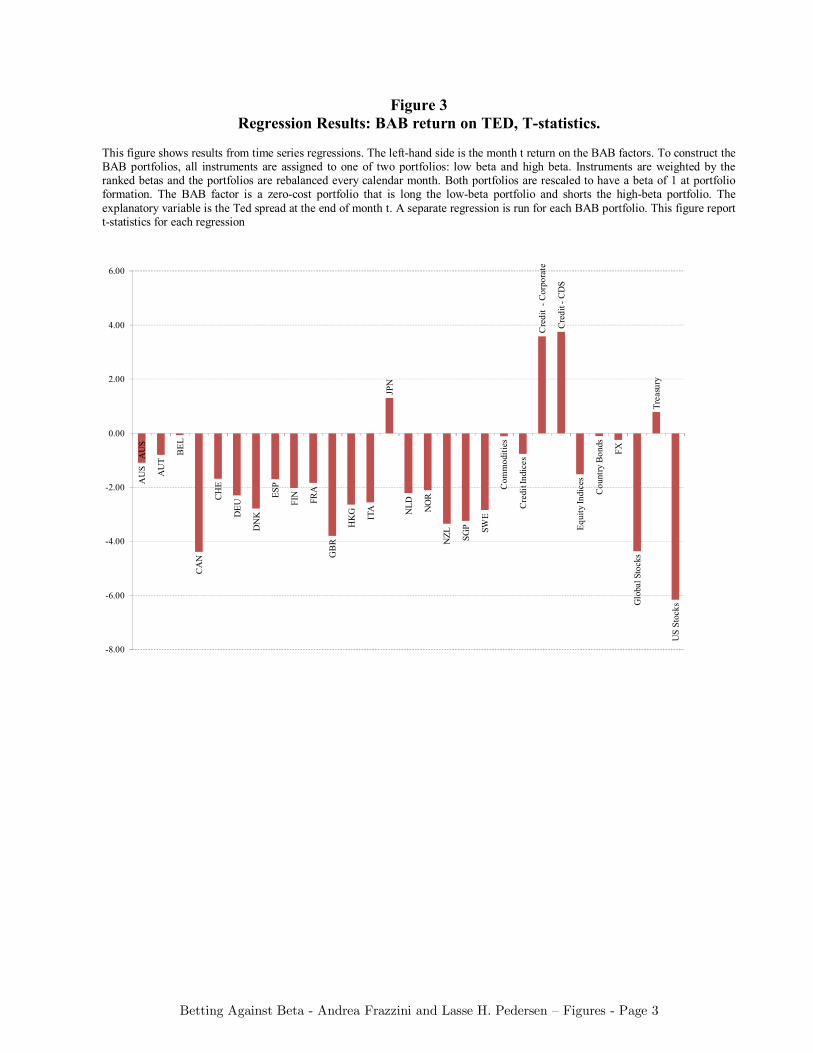
Betting Against Beta - Andrea Frazzini and Lasse H. Pedersen – Figures - Page 3
Figure 3 Regression Results: BAB return on TED, T-statistics.
This figure shows results from time series regressions. The left-hand side is the month t return on the BAB factors. To construct the BAB portfolios, all instruments are assigned to one of two portfolios: low beta and high beta. Instruments are weighted by the ranked betas and the portfolios are rebalanced every calendar month. Both portfolios are rescaled to have a beta of 1 at portfolio formation. The BAB factor is a zero-cost portfolio that is long the low-beta portfolio and shorts the high-beta portfolio. The explanatory variable is the Ted spread at the end of month t. A separate regression is run for each BAB portfolio. This figure report t-statistics for each regression
AU
S AU
T
BEL
CA
N
CH
E
DEU
DN
K
ESP
FIN
FRA
GB
R
HK
G ITA
JPN
NLD NO
R
NZL SG
P SWE
Com
mod
ities
Cre
dit I
ndic
es
Cre
dit
-Cor
pora
te
Cre
dit -
CD
S
Equi
ty In
dice
s
Cou
ntry
Bon
ds
FX
Glo
bal S
tock
s
Trea
sury
US
Stoc
ks
-8.00
-6.00
-4.00
-2.00
0.00
2.00
4.00
6.00
AU
S