This paper presents preliminary findings and is being distributed to economists

and other interested readers solely to stimulate discussion and elicit comments.

The views expressed in this paper are those of the author and do not necessarily

reflect the position of the Federal Reserve Bank of New York or the Federal

Reserve System. Any errors or omissions are the responsibility of the author.

Federal Reserve Bank of New York

Staff Reports

Betting against Beta (and Gamma)

Using Government Bonds

J. Benson Durham

Staff Report No. 708

January 2015

Betting against Beta (and Gamma) Using Government Bonds

J. Benson Durham

Federal Reserve Bank of New York Staff Reports, no. 708

January 2015

JEL classification: G10, G12, G15

Abstract

Purportedly consistent with “risk parity” (RP) asset allocation, recent studies document

compelling “low risk” trading strategies that exploit a persistently negative relation between

Sharpe ratios (SRs) and maturity along the U.S. Treasury (UST) term structure. This paper

extends this evidence on betting against beta with government bonds (BABgov) in four respects.

First, out-of-sample tests suggest that excess returns may have waned somewhat recently and that

the pattern seems most pronounced for USTs given data on ten other previously unexamined

government bond markets. Second, BABgov appears robust when hedged ex-ante against

covariance with equities and thereby does not resemble selling volatility, but these results

nonetheless belie a possible tension rather than consistency between leverage constraints and low-

risk investing: namely, that investors bid longer-dated UST prices higher (lower) under BAB

(RP). Third, the fact that Gaussian affine term structure models of USTs also imply an inverted

SR schedule suggests that investors cannot, in fact, realize abnormal returns if they are fully

hedged to the underlying model factors, and BABgov excess returns are indeed not robust to ex-

ante constraints on exposure to the yield curve’s principal components. Fourth, some evidence

suggests that previous BABgov results reflect coskew preferences, alternative BABgov strategies

hedged to coskew risks ex-ante forgo substantial returns, and there is no indication that investors

can earn excess returns betting against gamma. However, the sign of investors’ coskew

preferences in government bond markets remains ambiguous.

Key words: asset pricing, term structure, risk parity, betting against beta

_________________

Durham: Federal Reserve Bank of New York (e-mail: jbenson.durham@ny.frb.org). The author

thanks seminar participants at the Federal Reserve Bank of New York for helpful comments. The

views expressed in this paper are those of the author and do not necessarily reflect the position of

the Federal Reserve Bank of New York or the Federal Reserve System.

1  

Introduction

Mounting evidence suggests that low-risk investing delivers superior results, notably both across asset

classes, in the context of risk parity (RP), as well as within them, so-called “betting against beta” (BAB). Such

findings contradict the intuitive notion that higher expected as well as realized returns compensate investors

for taking risk, at least as measured by the second moment of asset returns. The effectiveness of these

investment strategies reflects a persistently inverse relation between Sharpe ratios (SRs) and beta, defined as

the covariance of asset returns with market portfolio returns, and correspondingly, an insufficiently upward-

sloped security market line (SML). Besides a comprehensive study of several asset classes that documents

these patterns (Frazzini and Pedersen, 2014), subsequent research reports that excess returns from BAB using

global equities are robust not only to size and momentum but also to industry classifications (e.g., Asness et

al., 2014).

Even though studies have long noted the modest slope of the SML (e.g., Black, 1972; Black et al.,

1972), which is surprising through the lens of the standard two-moment CAPM, the empirical literature on

low-risk investing seems far less extensive compared to other anomalies such as value, size, and momentum.

Moreover, arguably further analyses of any financial market anomaly tend to gravitate disproportionately to

risky assets, shares in particular.1 However, BAB results for the U.S. Treasury (UST) market (BABgov) are

among the most compelling, as only three of 28 other BAB strategies across asset classes have higher SRs,2

and the SR for BABgov, 0.81, is after all just as large if not greater in fact than that reported for U.S. equities,

0.78 (Frazzini and Pedersen, 2014).3 Given these compelling findings, analyses of low-risk investing might

evolve with equivalent attention to fixed income instruments,4 but to date this literature seems silent on just

why low-risk investing works for government bonds, the default-risk-free asset class, as distinct from the

mechanisms behind equity market behavior. Whatever the asset class, BAB should work as long as SRs

decrease in beta, and the salient features of the historical UST term structure data do seem amenable to the

strategy.5

Just why might compensation per unit of risk decline with maturity and thereby make BABgov

strategies profitable for investors who are willing and able to lever? The motivation for additional analyses of

BABgov transcends the obvious relevance for investors, and low-risk excess return patterns are noteworthy for

                                                            1 Compare the number of studies on, say, momentum in equity as opposed to bond markets. 2 Frazzini and Pedersen (2014) do not examine non-UST government bond markets. 3 Note, however, that the sample for equities (USTs) begins in 1926 (1952). Also, the corresponding excess return for BABgov is 17 bps per month (Frazzini and Pedersen, 2014, Table 6, pg. 14), compared with 70 bps for BAB using U.S. equities (Table 3, pg. 13), again given a longer sample for stocks. 4 Early indications seem consistent with prior patterns. For example, Baker et al. (2011), Asness et al. (2014), Chow et al. (2014), and Walkshäusl (2014) exclusively address the low-risk anomaly or BAB in the context of equities. 5 Duffee (2010), Fama and French (1993), and Campbell and Viceira (2001) each document high (low) SRs at the short (long) end of the curve.  

2  

monetary policymakers in at least two respects. First, a key mechanism underlying BAB excess returns are

leverage constraints, which have obvious implications for broader financial conditions. This notion advances

Black’s (1972) relaxed CAPM with restricted borrowing and suggests that a sufficient number of individual as

well as institutional investors, who notably seek high returns, are limited in their ability to borrow. These

restrictions thereby bid up prices on high-beta assets, concomitantly lower required returns, and flatten the

SML. BABgov patterns in particular highlight not the general level per se but the schedule of (relative) term

premiums across yield curves, an arguably neglected subject that can be relevant to market monitoring as well

as central bank open market operations. For example, the schedule of forward term premiums, or perhaps

rather SRs, seems highly relevant to central banks that endeavor to “remove duration risk” most efficiently

from financial markets with outright purchases of government bonds.6

Second, the underlying empirical regularity—again, elevated SRs at the front end of the term

structure—may represent a puzzle if not an affront to central bankers who painstakingly hone their

communication strategies. Investors might not only chronically require greater compensation per unit of

volatility around business cycle fluctuations but also amid corresponding uncertainty about the response of

monetary policy, quite possibly to varying degrees over time and across space. Therefore, the extent to which

SRs are greater at shorter maturities might be assessed in a similar vein as, for example, evidence that distant-

horizon forward rates are excessively sensitive to macroeconomic news announcements (Gürkaynak et al.,

2005), a finding that arguably reflects unanchored expectations around central bankers’ objectives. Evidence

on BABgov or simple analyses of SRs detailed further in subsequent sections below may be relevant in this

context. A reasonable prior might be that more inverted SR schedules correspond to less tightly moored

expectations around monetary policy goals or, perhaps more accurately, nearer-term objectives. Excess

BABgov returns, then, conceivably represent compensation for policy-related risks.

In addition to this shared relevance for investors and policymakers alike, four lingering questions

motivate an exclusive, closer look at BABgov. The first issue is the simple but pressing imperative to test

BABgov out of sample, which includes some further analyses of the U.S. data, including additional focus on

time-variation of returns, as well as an extension to 10 other previously unexamined government bond

markets, including Germany, France, Netherlands, Belgium, Italy, Spain, Japan, UK, Canada, and Switzerland.

Beyond assessing the breadth of the strategy, the cross-sectional evidence may help uncover conditional

information relevant to more efficient BABgov strategies.

The second issue stems from the general notion that the mechanisms that drive BAB may

fundamentally differ across asset classes, with possible implications for the broader, aggregate issue of RP.

Again, Frazzini and Pedersen (2014), drawing on Black (1972), argue that leverage aversion primarily

                                                            6 See, say, Bernanke (2010).

3  

generates the results. This mechanism seems persuasive within risky asset classes, but leverage aversion with

respect to government bond investors may appear at odds with RP itself, given the unique role of the (global)

risk-free asset class in portfolios.7 To consider any tension between BAB and RP, as well as to evaluate

flights-to-quality (FTQs) more broadly as an alternative or complementary explanation for BABgov, the

following further examines the covariance of BABgov not vis-à-vis the within-asset-class beta but with respect

to benchmarks that include the yardstick risky asset class.

Whereas additional evidence on BABgov covariance addresses possible mis-specification broadly

reminiscent of the Roll (1977) critique, a third issue regards potential under-specification. Gaussian affine

term structure models (GATSMs), a more common asset-pricing framework for government bonds than the

CAPM after all, nest BABgov but hardly imply that returns are anomalous. Closed-form solutions to

GATSMs are flexible enough to capture the inverted schedule between SRs and maturity (e.g., Duffee, 2010),

without the (however persuasive) amendments to the CAPM based on leverage aversion in Frazzini and

Pedersen (2014). The problem for BABgov as a proper anomaly is that GATSM-implied hedge ratios by

construction outlaw arbitrage and therefore excess returns, apart from portfolios formed from model-implied

fitting errors (e.g., Duarte et al., 2006). Levered portfolios that are long low-betas based solely on the

inverted SR schedule, and comprehensively hedged with respect to the underlying model factors, simply

cannot produce a free lunch. Perhaps no GATSM calibration comprises a satisfactory test given estimation

issues such a parameter stability and sample selection, but the affine model framework readily raises the

suspicion that any anomalous aspects of BABgov returns derive from an under-specified pricing kernel.

Simple regressions of ex-post BABgov returns on the principle components (PCs) of the term structure as well

as returns on portfolios that hedge broader exposure to PCs ex-ante are informative on this score.

The fourth issue addresses the fact that the “risk” in “low-risk investing” refers to the second and

not the third moment of asset returns. Beyond leverage aversion theory and other mechanisms, the following

examines whether BABgov returns owe in part to investors’ coskew preferences. Persuasive behavioral

arguments that might account for low-risk patterns for equities, including “over-confidence” and

“representativeness,” seem much less relevant for bonds. Nonetheless, BABgov portfolios may have

demonstrably favorable coskew characteristics that command a (negative) premium, which in turn may help

account for the low-second-moment risk phenomenon. Correspondingly, constrained BABgov strategies that

neutralize coskew exposures may generate lower returns. And, just as leverage-constrained investors may

reach for yield and thereby bid up prices to earn second-moment-based premiums, to boost gains they may

                                                            7 See also Adrian et al. (2014), the first study to conduct cross-sectional asset pricing tests that directly include in the pricing kernel measures of leverage, namely from financial intermediary balance sheet data from the Federal Reserve’s Flow of Funds data.

4  

similarly pressure required returns on assets with greater coskew risks lower. This begs the question of

whether investors can earn excess returns betting against gamma with government bonds (BAGgov).

Data and Empirical Design

These empirical analyses start with a brief evaluation of previous findings using Center for Research

in Security Prices (CRSP) data on USTs. Minor tweaks to Frazzini and Pedersen (2014) include use of daily

in addition to monthly data (as they do for stocks), market-capitalization-based instead of equal weights

across maturities, and alternative windows for estimation of the ex-ante (rolling) betas of 12 and 36 (12 and

59) months for the daily (monthly) frequency. The results also consider alternatives for shrinking the betas,

following Vasicek (1973),8 although the close relation between beta and maturity (and duration), as well as less

suspected measurement error of maturity, may suggest less need to make these adjustments for government

bonds. Also, the relevant betas are based on an aggregation of individual CUSIPs from the CRSP data into

eight maturity categories, which very closely but not precisely follows Frazzini and Pedersen (2014, Table 5,

pg. 14).9

Subsequent sections below examine strategies based on linear programming and non-linear

optimizations with key constraints, but the formation of the BABgov portfolios for this section follows the

convention introduced in Frazzini and Pedersen (2014), as in

1 1 1

1 1govBAB L f H ft t t t tL H

t t

r r r r r (1)

where 1 1

TL Ht t L Hr r w and

ˆ TL Ht t L Hw , with r ( ˆ

t )the column vector of returns (betas) for each

maturity, and rf is the risk-free rate (i.e., the one-month bill rate), as defined in Frazzini and Pedersen (2014)

and in turn Asness et al. (2014).10 All in all, daily (monthly) information is available for a sufficient cross

                                                            8 The shrinkage factor from Vasicek (1973) follows

ˆ ˆ ˆ1TS XSi i i iw w

with

12 2 2, ,1i i TS i TS XSw

where 2,i TS 2

XS is the time-series, TS, (cross-sectional, XS) variance of the estimated betas. Frazzini and Pedersen

(2014) cite this formula but fix 0.6iw , based on their results on U.S. equity data, and set ˆ 1XS for all assets, including USTs. 9 As noted in Table 2, these include 1 month to 9 months, 9 months to 2 years, 2 to 3 years, 3 to 4 years, 4 to 5 years, 5 to 6.5 years, 6.5 years to 12 years, and 12+ years. Varying UST issuance patterns present some challenges for covering some maturity buckets over extended periods. For example, the Treasury issued no 30-year bonds from November 1978 through February 1985. 10 Also,

5  

section of maturities from June 1961 (October 1957) through December 2013.11 Assuming a 12-month lag to

calculate L Ht based on daily (monthly) data, the first observation—the estimate of BABgov following (1) for

June 1962—is based on returns from June 1961 through May 1962. The final observation, December 2013,

refers to estimates of L Ht derived from returns observed from December 2012 through November 2013.

This produces a total of 620 months.

As noted previously, with the obvious motivation to explore the breadth of the strategy, the analyses

cover 10 additional government bond markets and use zero-coupon yield curves from Bloomberg.12 These

(monthly) data are only comprehensively available from around the mid-1990s, and therefore the inferences

additionally comprise out-of-sample temporal tests to a considerable degree.13 Also, the international panel

evaluates a broader scope of maturities,14 notably beyond the 10-year-plus category in Frazzini and Pedersen

(2014) to include the 20- and 30-year sectors in each case for a finer parsing of higher-beta maturities.15

Results: Sensitivity Analyses

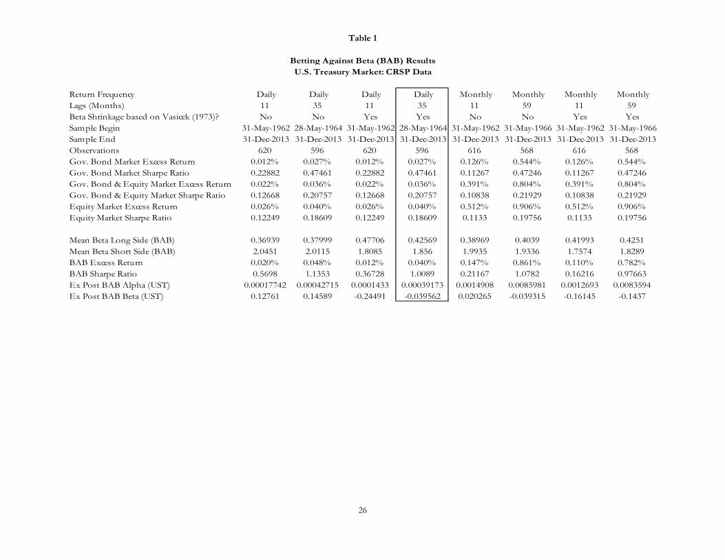
These modest revisions to the empirical design produce results that are largely consistent with

Frazzini and Pedersen (2014) with respect to USTs. Table 1 reports the results based on daily and monthly

returns using CRSP data, with and without shrinkage of the betas, and alternative lag lengths for estimation of

the betas, namely one and three years for daily data and one and five years for monthly data. Without

exception across these eight specifications, the SRs for BABgov exceed those on the UST index as well as the

stock market, and the excess returns in some cases are greater than those on shares. Although the results

using 1-year lags based on either daily or annual returns are less pronounced, the magnitude of the findings

                                                                                                                                                                                                

L Hw k z z

where 1'2 1nk z z

, itz rank , 1n denotes a vectors of ones of length n, and x+(-) indicate the positive

(negative) elements of the vector x. 11 Note that the results below refer only to monthly data from June 1961 to ensure consistency with the estimates based on daily data. However, earlier data do not meaningfully change the inferences. 12 Longer time series of fitted yield curves exist for a few cases, but Bloomberg perhaps provides the most comprehensive coverage for the purpose of consistent comparisons.

13 The Bloomberg (Index) mnemonics for, say, 10-year yields, are C91010Y (Germany), C91510Y (France), C92010Y (Netherlands), C90010Y (Belgium), C90510Y (Italy), C90210Y (Spain), C10510Y (Japan), C11010Y (UK), C10110Y (Canada), C25610Y (Switzerland), and C08210Y (U.S.). 14 To estimate realized returns on, say, the 10-year zero, further spline-based estimates of 9-year, 11-month zero-coupon yields are required, and the calculations otherwise follow Adrian et al. (2013). In addition, market capitalization weights are unavailable, and therefore the estimates of market returns assume equal weight across maturities, following Frazzini and Pedersen (2014). 15 Note also that Frazzini and Pedersen (2014) do not report data on the longest maturity bonds from August 1962 to December 1971. Also, lengthening the cross-section with finer delineations of duration might be very useful for asset-pricing tests.

6  

based on longer lags are similar to Frazzini and Pedersen (2014). For example, as noted in Table 1 as well as

Figure 1, daily data based on shrunk betas estimated with a 3-year lag, which implies 596 months of returns

from May 1964 through December 2013, produce an average (calendar-time, daily) excess return (SR) of

about 4.0 basis points (bps) (1.01), compared to 2.7 bps (0.47) for the UST market and 4.0 bps (0.19) for

equities. The long (short) side of the strategy on average has a beta of about 0.43 (1.85) or concomitantly a

required leverage ratio of 2.35 (0.54), and the ex-post beta (alpha) is very close to zero (positive), as expected

and consistent with Frazzini and Pedersen (2014). These results, in turn, reflect a clear underlying negative

relation between SRs (alpha) and maturity, which declines from about 1.359 (0.00017) to 0.214 (-0.00029)

from the 1M-9M to the 10Y+ maturity category, as noted in the top panel of Table 2.

Beyond this corroboration of previous results, time variation in BABgov returns merits further

consideration. Figure 1 also shows the rolling (geometric) 5-year mean return from the strategy, the black

line, which is notably lower toward the end of the sample and approaches zero, and indeed the SR from 1992

decreases to 0.74 from 1.01. Although not necessarily indicative of a “vanishing” or disappearing” anomaly

per se, a reasonable prior is that the results might not be as compelling for the cross-section of 10 other

markets, given that data are only available from the 1990s. Indeed, as noted in the last column of Table 3, the

corresponding Bloomberg data for the US (considering the 36-month estimation lag length for beta), which

again are monthly and also include the 20- and 30-year sectors, produce a lower SR (0.353) over the January

1995 to November 2014 sample. Then again, the returns to BABgov based on these limited Bloomberg data

nonetheless suggest a comparatively profitable strategy, as the SRs during this particular sample for the UST

and equity markets, as well as for a balanced portfolio,16 are clearly lower at 0.161, 0.129, and 0.196,

respectively. In addition, excess BABgov (calendar-time, monthly) excess returns are 61.6 bps, compared to

29.7, 57.4, and 43.6 bps, respectively.

However, the same cannot be said as assuredly for a number of other markets, and therefore the

results to BABgov may be somewhat sensitive to not only temporal but also spatial out-of-sample tests. Table

3 also reports that BABgov has a lower (greater) SR than the local government bond (stock) market in each of

the 10 cases. Also, BABgov excess returns exceed those on the corresponding equally-weighted government

bond in all cases except Canada, but the differences are arguably minimal compared to the U.S., with perhaps

the lone exception of data on Japan, which produces an excess return on BABgov of 50.2 bps, compared to

20.1 bps on the constructed government bond index over the sample. Also, BABgov excess returns are greater

than those on shares for six of the 10 non-U.S. cases—Germany, France, Netherlands, Belgium, Italy, and

                                                            16 The balanced portfolio is an equally-weighted average of returns on the local stock market, measured by the MSCI local currency, gross total return index (e.g., GDDU), and the government bond index, in turn an equally-weighted average of the 10 maturity points, which include 3 and 6 months as well as 1, 2, 3, 5, 7, 10, 20, and 30 years. The Bloomberg country (Index) codes follow GR (Germany), FR (France), NE (Netherlands), BE (Belgium), IT (Italy), SP (Spain), JN (Japan), UK (United Kingdom), CA (Canada), SZ (Switzerland), and US (United States).

7  

Spain—but on balance, these results seem to contrast meaningfully with those of the U.S., even allowing for

the differing temporal coverage of the CRSP and Bloomberg data. Furthermore, this general inference is

insensitive to assumptions regarding lag lengths, namely for 12- and 60-months, in addition to the 36-month

length for beta estimations summarized in Table 3.

To consider some explanations for the discrepancy, again BABgov profitability rests on a downward-

sloping schedule of SRs along the term structure, and as Figure 2 indicates, this pattern seems common but

perhaps not universal given this cross section of government bond markets. The schedule for the U.S.,

assigned to the back of the surface, is the most clearly downward sloping, but Germany, say, positioned at the

front, displays a noticeably less pronounced but nonetheless consistent pattern. In addition, Figure 3

corresponds to Figure 2 but focuses on comparisons with Germany, Japan, the U.K, and Switzerland and

shows a similarly inverse but weaker relation compared to the U.S. along the curve, which in turn reflects less

compelling BABgov excess returns.17 This cross-sectional evidence may be constructive in identifying

thresholds that signal abnormal BABgov returns, but the results also may motivate a closer examination of the

transmission mechanisms relevant for BABgov, or perhaps USTs in particular as a distinct global asset class.

More on Covariance: From FTQs to tension between BAB and RP

Indeed, the dearth of compelling evidence across other government bond markets might reflect

unique demand for longer-dated $U.S. denominated assets that transcends any leverage mechanism. Insofar

as longer- as distinct from shorter-dated USTs benefit from (global) safe-haven flows, or more precisely

provided investors anticipate this safe-haven demand, BABgov returns may owe less to leverage constraints

per se. In fact, some studies find that GATSM-based term premiums are negatively correlated with the VIX

(Li and Wei, 2012; Durham, 2008), or that jointly-estimated term and equity risk premiums are negatively

correlated (Durham, 2013a), findings that at first blush suggest that BABgov returns should be lower precisely

during “bad times.”18 However, this is only true if decreases in term premiums, notably scaled by risk, are

greater at the back end of the term structure. The results may hinge on investors’ perceptions and

expectations of the severity of shocks—during more benign FTQs, investors shed credit but not duration

exposure, whereas during more severe shocks they jettison both credit and duration risk for the relative safety

of short-dated government paper. The former (latter) would suggest that BAB does (does not) indeed

                                                            17 Higher SRs at the very front end of the US as opposed to other sovereign curves may owe more to the numerator rather than the denominator. At the very front end of the term structure, perhaps surprisingly, greater returns are a substantial part of the story, however further out the yield curve it appears that greater U.S. volatility plays the larger role. 18 Ilmanen (2011) argues that BAB returns resemble the profile of volatility selling, which pays off in “good” rather than “bad times.”

8  

resemble volatility selling.19 In any case, practitioners might worry that by underweighting the long end,

BABgov foregoes meaningful insurance against risky assets, and therefore excess returns reflect compensation

for such exposure.20

More broadly, the single-factor asset-pricing model behind previous BABgov results is possibly mis-

specified, perhaps broadly reminiscent of the Roll (1977) critique, not because the relevant market is

unobservable but rather given that the narrow within-asset-class betas behind BABgov exclude information

about covariance with the risky asset class. Two sets of rudimentary estimates are informative. The first is

simply to examine BABgov return loadings with respect to broader portfolios, , including, first, an market-

capitalization-weighted index of USTs and stocks from the CRSP dataset and, second, a pure equity portfolio,

as in

govBABt t tr r (2)

Table 2 also lists these results, namely the ex-post betas with respect to both measures of  for BABgov as

well as the eight maturity buckets, alongside the corresponding beta for the UST market index with respect to

. In short, BABgov appears to hedge against the balanced and equity portfolios just as well as, if not better

than, any sector of the term structure or the market as a whole. Both relevant betas are negative (-0.0054 and

-0.0041), whereas the remaining estimates along the term structure (from the 1-9 month to the 12-year pluse

categories) are strictly positive, albeit similarly close to zero. Of course, a covariance matrix might also

suffice, but these simple loadings seem inconsistent with the view that broader FTQs produce BABgov excess

returns.

The second constructs an alternative BABgov trading strategy that similarly levers (de-levers) the long-

(short-) side to have a beta of one as in Frazzini and Pedersen (2014), but under the linear programming

constraint that the long side has no greater beta with respect to, alternatively, the balanced or the pure equity

portfolio than the short side of the trade. More formally, the objective function and constraint follow

*

*

* *

ˆmin

.t .

ˆ ˆ

L

T

L tw

T T

L t S t

w

s

w w

(3)

                                                            19 Peso problems may lurk in the background, as it could be that even during a lengthy sample mild FTQs obtained, increasing the demand for longer- relative to shorter-dated Treasuries. What matters for BAB and leverage aversion is whether investors perceive longer-dated Treasuries as a better hedge against risky assets, which in turn depresses (expected) SRs further out the term structure. Therefore, instead of, or in addition to, leverage aversion, investors with balanced mandates may be paying an insurance premium. 20 Frazzini and Pedersen (2014) report within-asset-class ex-post BAB betas and do not address whether the long side has covariance properties that command positive premium. 

9  

where t is the vector of (UST, within-asset-class) betas along the term structure, the weights for the short

side follow

*

*,max

S

T

S t tw

w

, and t is the vector of betas with respect to the portfolios that include stock

returns.21 The returns follow

* *1 1 1* *

1 1ˆ ˆ

govT TBAB f f

t L t t S t tT T

L t S t

r w r r w r rw w

(4)

The resulting portfolio therefore is not only neutral to the UST market beta but also to the short side’s

covariance with .22 Put another way, (3) represents BAB, but without decreased relative protection against

stock market declines to achieve “low-risk government bond investing, without stock market covariance

bets.”

Consistent with the simple betas in Table 2, the results in Table 4 clearly suggest that BABgov does

not increase exposure to the yardstick risky asset class, and the results contradict the notion that BABgov owes

to FTQ-related preferences for longer-dated USTs. For example, the SRs for the constrained strategy with

respect to the balanced (stock) portfolio is 1.22 (1.09), which compares quite favorably with the results of the

unconstrained linear programming SRs of about 1.27. Also, the drag on average (daily) excess returns is

modest, with returns of 10.1 bps and 8.8 bps, compared to the unconstrained portfolio excess returns of 10.6

bps.23 Tables 6 and 7, which include the excess returns and SRs, respectively, for the constrained strategies

across the 10 additional government bond markets tell similar stories, with only a few exceptions. As such,

these results contradict the general notion that BAB constitutes volatility selling. Instead BABgov appears to

pay off just as well as a generic portfolio of USTs in “bad times.”

Arguably, these BABgov results constitute further crucial out-of-sample confirmation of RP, which

rests on “only one draw from history (though admittedly a fairly long one),” following Asness et al. (2012, pg.

48). However, even if the strategy does not appear to reflect selling volatility, BABgov may still represent a

                                                            

21 An equality constraint—e.g., * *ˆ ˆT T

L t S tw w —is too restrictive. The objective is to insure ex-ante that the

BABgov portfolio does not afford less of a hedge than the short side. 22 The linear programming constraint in effect forces the long side to include any sectors of the Treasury curve that hedge covariance at least as well as the short side. 23 In addition, the short end of the UST curve on average, but not always over the full sample, has a lower covariance with shares. That is, the constraint binds at times, evidenced by the fact that the average beta of the short side is about 0.584 (0.672), compared to the 0.200 average beta for the unconstrained portfolio. Also not the fact that returns are near zero for the most recent five years or so in the sample, when the long-end may have proved a decidedly better hedge with respect to shares near the zero lower bound. (In general, such a constraint is perhaps preferable to the ordinal weighting scheme for the standard BABgov portfolio, insofar as required leverage is much lower. Therefore, investors might consider linear-programming with stock market covariance constraints instead of the somewhat arbitrary weighting scheme in Frazzini and Pedersen (2014), which may exclusively serve to lower leverage requirements by adding relatively higher-beta assets to the long side.)

10  

special if not problematic case for RP. Consider investors who participate exclusively in the UST market, and

make all assumptions consistent with BAB. These participants may well overweigh the back end of the term

structure, increasingly so with leverage constraints. Such preferences push prices (yields) on, say, 10-year

USTs higher (lower), all else equal. Now consider another set of investors with balanced mandates who

participate in both the UST and the U.S. stock market. The same leverage constraints bind, but notably now

across rather than within asset classes, as in the broader context of RP. These investors may well overweigh

not longer-dated Treasuries but riskier shares to boost returns. Preferences push stock prices higher and

expected equity returns lower, but they also may pressure bond prices (expected returns) lower (higher) amid

“reaching for yield.” Therefore, investors with balanced mandates (and especially those also with longer-

duration liabilities) may offset those with narrower constraints, and heterogeneous preferences buffet longer-

dated yields. Without further clarification, BAB says leverage-constrained investors buy UST duration to

boost returns, whereas RP implies they sell it to do so,24 and the net effect on longer-dated yields appears

ambiguous. Unlike BAB evidence on risky asset classes, BABgov is perhaps not so much any confirmation as

a contradiction for RP, absent a complicated untold segmentation story that reconciles heterogeneous

investor preferences.25

GATSMs and Under-Specification

Besides mis-specification and tension between BAB and RP, also consider potential under-

specification. That is, although the CAPM and its extensions are common benchmarks for shares, the same

cannot be said for government bonds. Instead assess government bond SRs in the context of GATSMs,

which after all produce closed-form expressions for SRs (Duffee, 2010).26 Again, BAB works if SRs decrease

in beta (or duration), and the relevant analytical quantity is simply the partial derivative of SRs with respect to

maturity.27 Whereas the CAPM must be amended to incorporate borrowing constraints and capture the

relation, standard GATSMs do not. With the exception of some simplistic models, such as Merton (1973),28

calibrated GATSMs are flexible enough to produce downward-sloping SR schedules with respect to maturity,

but notably under conditions that preclude arbitrage. As such, the model parameters, particularly the generic

market price(s) of risk, might very well suggest more general mechanisms besides leverage aversion.

                                                            24 Indeed, Asness et al. (2012, pg. 49) note that under BAB “safer short-maturity U.S. Treasuries offer higher risk-adjusted returns than do riskier long-maturity ones” but “(w)ith respect to RP, bonds are the low-beta asset and stocks the high-beta asset, and the benefit that we documented is another empirical success of the theory.” 25 Baker et al. (2011, pg. 7) note that balanced fund mandates, without leverage constraint as well as perhaps beta rather than a market-weight allocation to shares, conceivably buy low-beta stocks (and presumably longer-dated Treasuries), but they also suggest that such mandates, at about two percent of the total, indeed hardly comprise the “representative investor” capable of realigning asset prices. 26 A GATSM might have a CAPM representation, but nonetheless the issue is under-specification of the pricing kernel. 27 As Frazzini and Pedersen (2014, pg. 3) note, term premiums exists at all horizons beyond the instantaneous short rate. 28 See Appendix 1.

11  

To repeat, BABgov results are based on a univariate asset-pricing framework (e.g., Frazzini and

Pedersen, 2014), but the literature on term structure models ubiquitously considers multiple factors, including

not just the level but also the slope and curvature of the term structure as well as other latent as well as

spanned and un-spanned macroeconomic factors. Moreover, and unfortunately for the prospects of a free

lunch, the observation that estimated GATSMs produce the salient features of the data, including SRs that

decline with maturity (Duffee, 2010), hardly confirms but rather precludes excess returns from BABgov.

Reconsider a BABgov strategy that is long the front end, PL, to exploit elevated GATSM-based SRs, with

corresponding short positions, PS, of required quantity, , to offset the exposure of the long side to each of

the underlying model factors, x.29 Instead of levering the long and shorts sides up and down to a beta equal

to one, as in (1), the hedge ratios, 1s and 2

s , for a 2-factor model, which can be trivially extended to n-

factors, follow

1

1 1

1 2 11

2 2 21

21 21

S S L

s

s S S L

n

nn n

P P P

x x x

P P P

xx x

(5)

But, these portfolio weights, very much akin to those in, say, Langetieg (1980), produce a certain return that

cannot exceed the risk-free rate without arbitrage (and in turn lead to the bond pricing equation). In other

words, the relevant partial derivatives on the right hand side of (4) are derived under the no-arbitrage

restriction, and therefore BABgov can only work by the coincidence that GATSM-implied yields are

persistently lower (higher) than observed yields at the front (back) end of the term structure, or if model

fitting errors are somehow a function of maturity. The very fact that GATSMs readily reproduce the required

SR schedule suggests that BABgov portfolios ultimately cannot produce excess returns, if comprehensively

hedged. Of course, to assert that any anomaly must compensative investors for some unknown but “true

risk” is unconstructive, but the issue is that GATSM-implied SRs may question more than confirm BABgov as

an anomaly per se.

Any empirical illustration of these restrictions, besides comprising a somewhat pedantic exercise, is

beset by the fact that arguably no calibration of a GATSM is satisfactory, given estimation issues such a

                                                            29 That is, the portfolio, which includes as many bonds as underlying risks, is L SP P , with the weights chosen to satisfy

0L SP P

x x

.

12  

parameter stability, not to mention sample selection in forming trading strategies.30 However, two simple

tests with much less structure might address some of the related issues, particularly that the asset-pricing

model on which BAB is based is not as much mis-specified, as in the case of covariance with risky assets, as

under-specified with respect to the multivariate nature of bond yields. The first is to examine BABgov return

loadings on the (first three) principal components of the yield curve,31 denoted by the vector tPC ,32

following

govTBAB PC PC

t t tr PC (6)

Table 2 also includes these results, and notably PC (0.0004) is safely significant within the 95

percent band and is just as large in magnitude as the corresponding estimate of ex-post with respect to

overall UST market returns (0.00039).33 Moreover, the loadings on each PC are within the range of estimates

of the corresponding ex-post betas for the eight sections of the yield curve, and therefore BABgov appears to

be robust, with no increased (contemporaneous) exposure to the underlying factors of the term structure.

However, a second test is more punishing and comprises an alternative BABgov trading strategy that

similarly levers (de-levers) the long- (short-) side based on the beta with respect to the UST market, but under

the constraint that the long and short sides have equivalent exposure to UST market PCs, following

*

*,

*, ,

ˆmin

.t .

ˆ ˆ

L

T

L t tw

T TPC PCL t t i t t

w

s

w w

(7)

where ˆ PCt is the n × m matrix of ex-ante beta exposures across the term structure to the first m PCs

estimated from t s to 1t , ,i tw is the market weight of the ith of n maturity categories at time t, and returns,

then, generally follow (4).34 The lower panels of Table 4 include the results for three constraints, including

                                                            30 In other words, one could examine whether the gap between GATSM-based fitted and observed yields—i.e., violations of the no arbitrage restriction—decline with duration, but uncertainty around parameter estimation and sample selection would complicate inferences from such an investigation. 31 Duffee (2010, pg. 3) suggests that GATSMs attribute the downward-sloping SRs to “level’ and “slope” risk. That is, “investors are compensated for the risk that the term structure jumps up; all bonds face this risk. Investors are also compensated for the risk that that slope of the term structure falls. Long maturity bonds hedge this risk, while short-maturity bonds are exposed to this risk.” If so, exposure to slope risk in particular might account for BABgov returns given the underweight to the back end of the yield curve. 32 The PCs are derived from 1-, 2-, 3-, 4-, 5-, 10-, 20-, and 30-year fitted zero-coupon yields over the full sample based on Gürkaynak et al. (2007). 33 Table 2 assigns 0 to alpha estimates within the 95 percent confidence interval. 34 That is, the PC betas for maturity category i follow

13  

slope (S); slope and curvature (S-C); and level, slope, and curvature (L-S-C). The SR for the strategy with the

slope beta constraint (0.387) is favorable with respect to either the stock or the UST market, but the figure is

much lower than that for the unconstrained BAB strategy (1.27), with substantially lower returns, 1.4 bps

compared to 10.6 bps (4.0 bps for the standard strategy). The tighter constraints that include curvature as

well as level exposure produce minimal excess returns, 0.4 bps and 0.2 bps, respectively, and unremarkable

SRs. In addition, the cross-sectional evidence similarly suggests that PC-based constraints are punitive, as the

SRs listed in Table 6 under the S, S-C, and L-S-C constraints are negligible. Tellingly also, the weighted betas

of the long sides given ex-ante hedges for slope and curve—not to mention for the level, slope, and curve—

increasingly approach unity, which may simply suggest that investors cannot simultaneously BAB and hedge

these PCs to meaningful effect. Thus in short, although ex-post BABgov returns do not seem to load on

contemporaneous PCs, ex-ante hedges against exposure to the underlying PCs appear very costly, which in

turn raises questions about under-specification. Yet whatever these empirical results, again GATSM-implied-

downward-sloping SR schedules do not necessarily imply excess BABgov returns.

Skew Preferences

The previous discussion of mis- and under-specification is confined to “risk” with respect to the

second moment of returns. Another consideration regarding BAB in general as well as BABgov in particular is

investors’ skew preferences,35 which might but need not necessarily stem from managerial delegation.36

Indeed, the literature on third-moment preferences with reference to flat SMLs and high risk-adjusted returns

on low-second-moment-risk assets is hardly new. As Kraus and Litzenberger (1976) reported in their early

study of the three-moment CAPM, higher beta portfolios exhibit greater market coskew, which in turn

requires a premium that might account for the lower-than-expected second-moment-based slope of the

                                                                                                                                                                                                

, , ,

TPC PCi t i i t t i tr PC

where t refers to the alternative lagged windows. An ex-ante slope beta, for example, is the coefficient on the regression of, say, 2- to 3-year maturity returns on the second PC of the yield curve, estimated over the, say, 12-month rolling window. 35 Another possible explanation for abnormal returns on low-risk assets refers to delegated management incentives, namely benchmarking (Baker et al., 2011), arguably representative of a broad limit to arbitrage. Although absolute risk, or rather covariance with marginal utility, should matter for investors, typical industry practice is to assess managerial skill with respect some benchmark. In turn, although low-risk strategies produce quite favorable SRs, information ratios (IRs) may pale in comparison, and therefore even “smart” managed money does not offset the price impact of (irrational) demand for high-beta assets. 36 More recently, Taleb (2004) makes the opposite case for negative skew preferences, but only partially in the context of delegated asset managers who prefer “blowups” over “bleeding.” To the extent that the representative investor conforms to utility functions broadly consistent with prospect theory, the agent-based mechanisms that Baker et al. (2011) describe are neither necessary nor sufficient conditions for BAB.

14  

SML.37 Expected excess returns, eiE r , are a function of not only covariance with market portfolio returns

but also coskew, with 0 , as in

3ˆ ˆei i i mE r sign M (8)

where follows

2

3

covˆ

i m m

i

m m

r r

E r

(9)

and 3mM is the third central moment of market returns.38 Kraus and Litzenberger (1976) posit that high beta

is a source for gamma,39 and as such BAB might seem less anomalous in the context of a higher-moment

CAPM.40 Thus, low-risk investing with respect to the second moment of returns might comprise high-risk

investing regarding the third, and the literature does not address whether BABgov might embed coskew risks.41

Even so, much of the intuition for skew preferences for risky asset classes seems less germane to

government bonds, given the usual focus on the potential for exceptional upside rather than downside

protection. For example, Mitton and Viorkink (2007) find that volatile stocks are more positively skewed,

and therefore command higher prices, owing to their lottery-like potential cash flows. To a large degree,

these mechanisms stem from “representativeness,” which hardly seems relevant to longer-dated Treasuries

that may benefit from FTQs. Consider also the literature that invokes “overconfidence” in the context of

skew. Diether et al. (2002) argue consistent with Miller (1977) that, given impediments to short selling,

                                                            37 Transaction costs are another consideration under this general rubric, and indeed bid-ask spreads can be particularly punitive at the very short end of the UST bill curve (Duffee, 2010), again where the long side of BAB Treasury portfolios are notably overweight. But at the same time, as Duffee (2010) and Figure 4 illustrate, the inverse relation between SRs and maturity (or beta) is more monotonic than discontinuous and does not owe exclusively to the front end. In addition, the results in Frazzini and Pedersen (2014) do not rest on exclusively overweighing the shortest maturities, as instead the low and the high beta portfolios include every sector along the term structure, albeit with greater weights on the extremes. 38 See Appendix 2 for rudimentary measurement details. 39 Kraus and Litzenberger (1976, pg. 1098) regress gamma on beta and report a coefficient greater than unity (i.e., 4.5), and they infer that “investors have an aversion to increases in beta as a direct measure of systematic standard deviation and have a preference for increases in beta as a surrogate for proportionally greater increases in systematic skewness (given positive market skewness).” 40 An analogous explanation for BAB success with respect to shares refers to the observation that high-beta, volatile stocks also tend to be small and illiquid, which presumably in the context of Baker et al. (2011) suggests that institutional investors cannot exploit the anomaly. An alternative reasoning, as the following outlines, is that skew preferences for lottery-like payoffs account for lower expected returns. 41 Put another way, explicit consideration of the coskew of BAB returns should shed light on the extent to which leverage constraints drive the anomaly, as Ilmanen for example pits leverage constraints and skew preferences as alternative explanations.

15  

optimists’ influence over stocks prices increases with uncertainty, evidenced by disagreement among

investors. Therefore, volatile high-beta stocks are overbid to the extent optimists disproportionately set

prices, again under the assumption that otherwise offsetting investors have a general reluctance or inability to

short stocks, notably not inconsistent with leverage aversion.42 The same mechanism may work for longer-

dated Treasuries, but the logic contradicts the documented positive empirical correlation (and analytical result

from GATSM closed-form solutions) between uncertainty and term premiums (i.e., required returns over

short rates). Convention suggests that greater volatility lowers, rather than increases, expected returns in

government bond markets.

Nonetheless, coskew preferences may help account for BABgov, but through distinct channels.43 It

may seem de rigueur to test whether any fixed-income arbitrage strategy resembles “picking up nickels in

front of steamrollers (Duarte et al., 2006),” but more importantly, fixed income securities may have

fundamental characteristics that generate asymmetric return distributions, as of course bond prices (nominal

interest rates) face an upper (lower) bound at par (zero). In addition, “pull to par” is arguably more

pronounced nearer the short end of the term structure, which may be especially relevant for BABgov. In fact,

Fujiwara et al. (2013) report conditional negative skew using daily government bond excess returns,

particularly at shorter maturities,44 which may imply greater second-moment-based SRs at shorter horizons

consistent with BABgov. Also, Durham (2008) argues that expected returns, as measured by ex-ante GATSM-

based term premiums in the U.S., positively correlate with Eurodollar-option-implied short-term-interest-rate

skew but does not address the schedule of SRs.45 Yet to be sure, coskew rather than unconditional skew

should affect asset returns. The question is whether the coskew of longer-dated bonds makes them pay off

disproportionately well, again per unit of duration risk, compared to shorter-dated securities in “bad times”

amid asymmetric shocks to both the risk-free and the risky asset classes. The coskew of returns—both within

the Treasury market, as in the BAB evidence, or across asset classes, more relevant to RP—may complement

                                                            42 See Hong and Sraer (2012) also in this general context. 43 The argument is not that the back end of the Treasury curve has (potential) lottery-like return characteristics. But perhaps in contrast to Ilmanen (2011, pg. 389), downside protection from Treasuries might nonetheless manifest through coskew preferences, in addition to volatility, correlation, and jump premiums. 44 Even so, they also find that the Bowley coefficient, defined in Appendix 2 as a measure of skew nearer the center of the distribution and notably further from the tails, is often positive, which suggests that negative standard skew in the sample owes to outliers (i.e., the small probability of a large and negative excess return). 45 Three-moment CAPM tests for USTs are also informative with respect to the ubiquitous use of GATSM, in which by definition skew cannot be priced.

16  

or supplant leverage aversion theory behind BABgov,46 as investors may not be so much reaching for yield

amid leverage constraints as paying for their preferred coskew exposure.47

Two benchmarks for coskew are relevant, which reflects the previous discussion of covariance. The

first is within asset classes, to follow Frazzini and Pedersen (2014), and the second is across them, which

addresses the notion that skew preferences may operate through broader (balanced) asset allocation channels.

From a practitioner’s perspective, the question is whether BABgov unwittingly entails coskew risks, with

respect to either the UST or the stock market, and toward that end, Table 2 also reports BAB coskew with

different tenors along the government bond curve. Considering the UST benchmark first, again to address

directly the original BAB findings, tends to increase with maturity, not unlike , and ranges from an ex-post

(ex-ante) estimate of 0.50 (0.87) for the 1-to-9-month category to 1.86 (1.40) for the longest duration

category. Notably, the ex-post estimate is 0.44 for the BABgov portfolio, and the key issue is contribution to

unconditional UST market portfolio skew, which is positive according to both standard (0.536) and Bowley

skew (0.093) measures.48 Therefore, under the conventional assumption that investors prefer positive

portfolio skew, commands a negative premium,49 and as such skew preferences may help account for

previous BABgov results (Frazzini and Pedersen, 2014), because longer maturities best contribute to the

overall positive tilt of UST market returns over this sample.  

However, beyond the initial BABgov results, the second broader set of benchmarks imply no clear

inference, as the corresponding estimates of with respect to the broader balanced portfolio of bonds and

stocks produce ambiguous relations. BABgov returns have negative coskew with the balanced portfolio (-

.0572), which has negative unconditional standard (-0.973) as well as Bowley skew (-0.069), and thereby

implies a positive premium. Also, the for BABgov is safely within the range across the term structure (from -

0.102 for the 3Y-4Y sector to -0.014 for the 1M-9M category).

Arguably, the contribution of BAB to broader balanced portfolio skew as opposed to UST market

skew is the more relevant consideration for practitioners, particularly with balanced mandates, but the former

results are nonetheless relevant to the original BABgov evidence. In any case, besides ex-post BABgov returns,

                                                            46 Note that on average if longer-run Treasuries favorably contribute to portfolio coskew, they must have positive coskew when the market is skewed positively and negative coskew when the market is skewed negatively. Both scenarios command a premium—i.e., lower yields (higher prices) for duration—as Treasury duration reinforces benevolent positive skew in the first case but offsets undesirable negative skew in the second. 47 The results and motivation from Barone-Adesi et al. (2004) might be analogous. They report coskew characteristics that command a positive (negative) risk premium and thereby account for abnormally high (low) small (large) cap stock returns, in perhaps the same way coskew might help account for BABgov excess returns. 48 This finding is also consistent with Chiang (2008), who uses monthly data from 1976 through 2005 on a broader set of U.S. fixed income sectors, including USTs, corporate bonds, and MBS. 49 The negative conditional skew on BAB returns (-0.09) is broadly consistent with “picking up nickels in front of steamrollers,” whereas all points on the term structure are positively skewed. But, the Bowley coefficient is positive, and besides, coskew matters for asset pricing.

17  

another imperative is to evaluate the cost of hedging coskew risk ex-ante, similar to the covariance and PC

exposures discussed previously. Table 7 reports the results from constrained optimizations from “low-risk

government bond investing without coskew bets.” These portfolios are long low-beta bonds as before, but

subject to the constraint that the long and short sides have a weighted-average of unity to match the market

portfolio. The constraints follow both linear programming as well as non-linear optimization. The long side

for the former constraint, given that is additive like (Kraus and Litzenberger, 1976, pg. 1089), follows50

*

*,

* 1, , ,

1

ˆmin

.t .

ˆ ˆ 1

L

T

L t tw

nT

L t t i t i ti

w

s

w n w

(10)

where t̂ is the vector of estimates across the term structure, and ,i tw is the market weight of the ith of n

duration buckets at time t. The long side for the latter optimization, with the same objective function and a

non-linear equality constraint, follows

*

*,

2*, , ,

3

, ,

ˆmin

.t .

cov1 0

L

T

L t tw

T

L t t m t m t

m t m t

w

s

w r r

E r

(11)

where tr is the n × 1 vector of returns across the term structure, and ,m tr is the corresponding market return

with mean ,m t .51

                                                            50 Correspondingly, the objective function and the linear constraint for the short side follow

*S

*S,

* 1S, , ,

1

ˆmax

.t .

ˆ ˆ

T

t tw

nT

t t i t i ti

w

s

w n w

51 Similarly, the objective function and the linear constraint for the short side follow

*S

*S,

12 3*

S, , , , ,

ˆmax

.t .

cov 1 0

T

t tw

T

t t m t m t m t m t

w

s

w r r E r

 

18  

The results suggest a meaningful drag on excess returns, with an offsetting decline in volatility that

still results in favorable SRs. As listed in Table 7, BABgov excess returns with non-linear (linear) gamma

constraints with respect to the UST market is about 1.2 (1.7) bps per month, compared to 10.6 (4.0) bps per

month for the unconstrained (standard) strategy. The SR is about 0.40 (0.58), compared to 1.27 (1.01) for the

unconstrained portfolio (standard method). The results are similar given the balanced portfolio benchmark,

and the costs of the ex-ante coskew hedge are evidenced by an excess return of 1.3 (1.6) bps per month under

the nonlinear (linear) constraints, with a corresponding SR of about 0.40 (0.41). Returning to Tables 6 and 7,

the results are broadly similar for the cross-section of government bond markets, although perhaps the

reduction in excess returns and SRs are somewhat more pronounced compared to the corresponding

unconstrained optimizations.

Betting against gamma (BAG) and the market price of coskew risk

These results on the third-moment risks of BABgov portfolios are somewhat ambiguous. On the one

hand, some results suggest that BABgov excess returns (Frazzini and Pedersen, 2014) do compensate investors

for coskew exposure, but on the other, Table 7 also suggests some residual excess returns to the strategy. Yet

another natural and related empirical question is whether, similar to beta, investors can bet against gamma

(BAG). Just as BAB is long “low risk,” so is BAG, but with respect to the third as opposed to the as second

moment. Instead of shorting high-beta assets, the trading strategy is to short assets with positive (negative)

coskew, but only when unconditional market skew is negative (positive). The corresponding long side

overweighs assets with negative (positive) coskew when market skew is unconditionally negative (positive).

To grasp intuition further, recall that under leverage constraints investors reach for yield and bid up

prices of high-beta assets, more formally given that 0 . By similar logic given the same leverage

aversion, if skew preferences are also priced with 0 , then to earn further premiums and boost returns

under constraints, investors might similarly overprice assets that have positive (negative) coskew with the

market when the market is negatively (positively) skewed, all else equal. The long side of another trading

strategy follows

*

*

* 3, ,

* 3, ,

*,

ˆmin 0

ˆmax 0

.t .

ˆ 1 0

L

L

T

L t t m tw

T

L t t m tw

T

L t t

w if M

w if M

s

w

(12)

19  

with the converse conditions for the short side,52 and the return (given that both the long and short sides

have market betas) is

* *1 1 , ,

gov TBAGt t L t S tr r w w (13)

A similar approach closer to the canonical BAB tests follows

31 1 ,

13

1 1 ,

1 10

ˆ ˆ

1 10

ˆ ˆ

gov

T Tf fL t H t m tT T

L t H tBAGt

T Tf fL t H t m tT T

L t H t

w r r w r r if Mw w

rw r r w r r if M

w w

(14)

where analogous to (1), L Hw k z z , 1'2 1nk z z

, and ˆ

itz rank . Not unlike the linear

constraints to the optimizations, the weights 1

ˆT

tL Sw

on the long and short sides ensure that BAGgov

portfolios have a market beta equal to one.53 Figure 4 shows the results based on (14) using the daily CRSP

data, from June 1961 through December 2013, with a 3-year rolling window for estimation of covariance and

coskew. Also, Figure 5 shows the corresponding results, but with respect to an alternative measure of

coskew, SKD from Harvey and Siddique (2000). Clearly, there is no evidence of excess returns to the strategy

in either case, and none of the 10 other government bond markets produce meaningful excess returns to

BAG.

Keep in mind, however, that the motivations for BAGgov as well as the hedges in the previous section

assume preferences for positive portfolio skew. A remaining question is whether a three-moment CAPM,

which clearly is not preference-free and instead requires that investors are risk-averse with non-increasing

absolute risk aversion, in fact holds over the sample. That is, do investors indeed demand a negative

(positive) premium for positive (negative) coskew when the UST market is positively (negatively) skewed?

Toward that end, Figure 6 shows the covariance-coskew-excess return surface for eight maturity categories

                                                            52 That is, the objective and the linear constraint for the short side follow

*S

*S

* 3S, ,

* 3S, ,

*S,

ˆmax 0

ˆmin 0

.t .

ˆ 1 0

T

t t m tw

T

t t m tw

T

t t

w if M

w if M

s

w

53 Given that range of across the term structure, unlike the distribution of (non-negative) s, straddles the origin, leveraging to a of unity is not mathematically feasible.

20  

along the term structure, where and are measured with respect to the UST portfolio using monthly data

from June 1961 through December 2013. As expected and by visual inspection, the plane is positively sloped

with respect to , albeit perhaps moderately so, consistent with previous findings such as Black (1972).

However, the slope vis-à-vis 3msign M is also positive, notably perversely so considering the positive

unconditional skew of UST market returns over the full sample. Figure 7, which measures covariance and

coskew with respect to the balanced portfolio and includes the SKD measure (Harvey and Siddique, 2000)

instead of , implies the same problematic inference. If investors prefer positive coskew, the surfaces in

Figures 3 and 4 should be downward-sloping in 3msign M and SKD, respectively.

In addition to this informal evidence, simple asset-pricing tests based on regressions follow

3, , ,t : 1 , , : 1 , : 1 ,

ˆ ˆei t t t i s t t i t s t m t s t i tr sign M (15)

with the Null hypotheses 0 and 0 , where ˆi and ˆ

i for the ith asset as well as 3mM , the

unconditional standard market skew, are estimated from returns from t s to 1t .54 Table 8 reports the

results given the UST market as the benchmark index using alternative lag lengths of 12 and 36 months as

well as a pure cross-sectional design with , , and SKD estimated over the complete sample period, with and

without shrinkage of and , and given both daily and monthly return data. Similarly, Table 9 shows the

results that correspond to the balanced portfolio of USTs and stocks as alternative benchmarks. Given the

small Fama-Macbeth (1973) t statistics on in each case, as well as some perverse positive coefficient

estimates, the clear inference is that coskew does not, after all, seem to be priced following the standard three-

moment CAPM. Then again, the estimates, which have the expected positive sign more consistently, are

nevertheless not statistically significant, either. These ambiguous results, which are not dissimilar to previous

findings for a broader cross-section of bonds (Chiang, 2008) but inconsistent with the general evidence that

0 from Kraus and Litzenberger (1976) and Friend and Westerfield (1980),55 raise some questions about

the motivations for BAG and hedging coskew risks. At the same time, they do not necessarily comprise

                                                            54 The alternative in the lower panels of Tables 9 and 10 follow Harvey and Siddique (2000), as in

, , ,t : 1 , , : 1 ,ˆe SKD

i t t t i s t t i t s t i tr

 55 Friend and Westerfield (1980), however, question the broader inference in Kraus and Litzenberger (1976) that the addition of coskew preferences largely accounts for previous violations of the two-moment CAPM, including that the implied risk-free rate is distinguishable from the actual risk-free rate.

21  

corroboration of, say, Taleb’s (2004) alternative view that investors prefer negative coskew, which draws from

the effects of small samples of observed returns,56 prospect theory (PT),57 or hedonic psychology.58

Summary

As Frazzini and Pedersen (2014) as well as Asness et al. (2012, 2014) and others note, the magnitude

of BAB excess returns, notably including published returns for BABgov in particular, are perhaps as

compelling as for any other apparent violation of asset pricing theory such as size, value, or momentum.

Given motivations for investors and central bankers alike to understand the price and quantity of risk along

the term structure, the preceding analyses devotes exclusive attention to BABgov with respect to simple out-

of-sample tests, further consideration of covariance with risky assets, a broader specification of the underlying

asset pricing model more consistent with GATSMs as opposed to the single-factor CAPM, and coskew with

respect to both the risk-free, relevant to BAB, and risky asset classes, germane to RP.

On balance, the results are somewhat mixed. BABgov returns do appear to have diminished

somewhat in recent decades, especially during the last five years. This trend in turn might owe to the post-

crises experience with the zero lower bound for nominal interest rates and unconventional policy measures,

to the extent that central bankers have pinned down short rates and decreased their near-term sensitivity to

macroeconomic news, or given the “portfolio-rebalancing” channel in which large scale asset purchases

(persistently) push down longer-dated UST yields.59 In addition, some evidence also suggests that the

phenomenon might be largely confined to USTs, which may question the universal application of leverage

aversion theory behind BAB or highlight the possibly unique role for USTs as a global safe-haven asset.

Even so, BABgov returns do not appear to compensate investors for special FTQ-related demand for USTs at

the back as opposed to the front end of the term structure. Instead, alternative BABgov trading strategies with

simple linear programming constraints to hedge covariance with stock returns tend to produce not only

nearly as favorable risk-adjusted results but also comparable absolute excess returns.

If anything, more evidence suggests that BABgov compensates investors for coskew rather than

covariance risks, but lucid conclusions are hard to draw. Some results suggest that ex-post BABgov excess                                                             56 Skew exacerbates the “small numbers” effect, because the observed mean (variance) will differ from (be lower than) the observed mean (variance). 57 The value function of PT implies decreased sensitivity to both gains and losses and therefore an overall preference for negative skew. Agents under PT are more concerned with changes than with accumulated wealth, as the value function is concave (convex) in the profit (loss) domain (and the value of a large loss is greater than the corresponding sum of losses). 58 The central notion in hedonic psychology is that agents soon revert to a “set-point of utility” after some shock, as again changes in utility rather than absolute (cumulative) levels affect preferences, and similar to PT, the implied value function is concave (convex) in the profit (loss) domain. 59 The Federal Reserve’s maturity extension program announced on September 21, 2011—otherwise and informally known as an “operation twist two”—might also affect BABgov returns by depressing expected returns at the back end of the term structure, all else equal.

22  

returns reflect a negative premium for coskew, but curiously perhaps with respect to the UST market (e.g.,

Frazzini and Pedersen, 2014) as opposed to a broader portfolio of bonds and shares. Ex-ante hedges to

neutralize coskew risks with respect to either market proxy, unlike the results for covariance, appear to be

costly in terms of foregone excess returns. But to muddy the waters further, standard asset pricing tests do

not seem to support the three-moment CAPM for these data, and therefore such hedges may be unwarranted

if investors in fact have neither positive (Kraus and Litzenberger, 1976) or negative portfolio skew

preferences (Taleb, 2004). In addition, BAGgov does not seem to produce excess returns, hedged for

underlying beta exposure. Whatever these results, “low-risk” investing refers to second- rather than third-

moment risks, and further analyses of BAB should arguably test for coskew preferences routinely.

The previous discussion does not fully address managerial delegation and benchmarking as another

explanation for BABgov returns, following Baker et al. (2012). Indeed, returning to Table 2, the information

ratios (IRs) (0.19) for even the most profitable strategies are unremarkable, which might help explain why a

meaningful number of institutional investors do not exploit these favorable patterns. However, a low IR is

neither a necessary nor sufficient condition to explain favorable absolute-risk-adjusted returns. Perhaps the

most problematic result for BABgov is that, although the ex-post loadings appear favorable, as they do for

term structure momentum (Durham, 2013b), the ex-ante hedges for level, slope, and curvature exposure

largely erase the gains from the strategy, using both the CRSP data on USTs and the Bloomberg data on the

broader cross-section. Again, as argued previously, the fact that GATSM parameters may readily reproduce

an inverse schedule between SRs and maturity does not imply abnormal BABgov returns, but rather to the

contrary that such an empirical relation is not necessarily inconsistent with the no-arbitrage condition.

23  

References

Adrian, Tobias, Richard Crump, and Emanuel Moench, 2013, “Pricing the Term Structure with Linear Regressions,” Journal of Financial Economics, vol. 110, pp. 110–138.

Adrian, Tobias, Erkko Etula, and Tyler Muir, 2014, “Financial Intermediaries and the Cross-Section of Asset Returns,” Journal of Finance, vol. 69, no. 6, pp. 2557–96.

Asness, Clifford, Andrea Frazzini, and Lasse H. Pedersen, 2014, “Low-Risk Investing without Industry Bets,” Financial Analysts Journal, vol. 70, no. 4, pp. 24–41.

Asness, Clifford, Andrea Frazzini, and Lasse H. Pedersen, 2012, “Leverage Aversion and Risk Parity,” Financial Analysts Journal, vol. 68, no. 1, pp. 47–59.

Baker, Malcom, Brendan Bradly, and Jeffrey Wurgler, 2011, “Benchmarks as Limits to Arbitrage: Understanding the Low-Volatility Anomaly,” Financial Analysts Journal, vol. 67, no. 1, pp. 40–54.

Barone Adesi, Giovanni, Patrick Gagliardini, and Giovanni Urga, 2004, “Testing Asset Pricing Models with Coskewness,” Journal of Business and Economic Statistics, vol. 22, no. 4, pp. 474–485.

Baz, Jamil, and George Chacko, 2004, Financial Derivatives: Pricing, Applications, and Mathematics, Cambridge University Press.

Bernanke, Ben, 2010, “The Economic Outlook and Monetary Policy, speech at Jackson Hole, Wyoming.

Black, Fischer, 1972, “Capital Market Equilibrium with Restricted Borrowing,” Journal of Business, vol. 45, no. 3, pp. 444–455.

Black, Fischer, Michael C. Jensen, and Myron S. Scholes, 1972, “The Capital Asset Pricing Model: Some Empirical Tests,” In Studies in the Theory of Capital Markets. Edited by Michael C. Jensen. New York: Praeger.

Campbell, John Y. and Luis M. Viceira, 2001, “Who Should Buy Long Term Bonds,” American Economic Review, vol. 91, no. 1, pp. 99–127.

Chow, Tzee-man, Jason C. Hsu, Li-Lan Kuo, and Feifei Li, 2014, “A Study of Low-Volatility Portfolio Construction Methods,” Journal of Portfolio Management, vol. 40, no. 4, pp. 89–105.

Chiang, I-Hsuan Ethan, 2008, “Skewness and Co-skewness in Bond Returns,” working paper, Boston College.

Diether, Karl B., Christopher J. Malloy, and Anna Scherbina, 2002, “Differences of Opinion and the Cross Section of Stocks Returns,” Journal of Finance, vol. 57. no. 5, pp. 2133–2141.

Duarte, Jefferson, Francis Longstaff, and Fan Yu, 2007, “Risk and Return in Fixed-Income Arbitrage: Nickels in Front of a Steamroller?” Review of Financial Studies, vol. 20, no. 3, pp. 769–811.

Duffee, Gregory R., 2010, “Sharpe Ratios in Term Structure Models,” working paper.

Durham, J. Benson, 2008, “Implied Interest Rate Skew, Term Premiums, and the ‘Conundrum,’” Journal of Fixed Income, vol. 17, no. 4, pp. 88–99.

24  

Durham, J. Benson, 2013a, “Arbitrage-Free Models of Stocks and Bonds,” Federal Reserve Bank of New York Staff Reports, no. 656.

Durham, J. Benson, 2013b, “Momentum and the Term Structure of Interest Rates,” Federal Reserve Bank of New York Staff Reports, no. 657.

Gürkaynak, Refet S., Brian P. Sack, and Eric T. Swanson, 2005, “The Sensitivity of Long-Term Interest Rates to Economic News: Evidence and Implications for Macroeconomic Models,” American Economic Review, vol. 95, no. 1, pp. 425–436.

Gürkaynak, Refet S., Brian P. Sack, and Jonathan Wright, 2007, “The U.S. Treasury Yield Curve: 1961 to the Present,” Journal of Monetary Economics, vol. 54, no. pp. 2291–2304.

Fama, Eugene F. and Kenneth R. French, 1993, “Common Risk Factors in the Returns on Stocks and Bonds,” Journal of Financial Economics, vol. 33, pp. 3–56.

Fama, Eugene F. and James D. MacBeth, 1973, “Risk, Return, and Equilibrium: Empirical Tests,” Journal of Political Economy, vol. 81, no. 3, pp. 607–636.

Frazzini, Andrea and Lasse Heje Pedersen, 2014, “Betting Against Beta,” Journal of Financial Economics, vol. 111, pp. 1–25.

Friend, Irwin and Randolph Westerfield, 1980, “Co-Skewness and Capital Asset Pricing,” Journal of Finance, vol. 35, no. 4, pp. 897–913.

Fujiwara, Ippei, Lena Mareen Korber, and Daisuke Nagakura, 2013, “Asymmetry in Government Bond Returns,” Journal of Banking and Finance, vol. 37, pp. 3218–3226.

Harvey, Campbell and Akhtar Siddique, 2000, “Conditional Skewness in Asset Pricing Tests,” Journal of Finance, vol. 55, no. 3, pp. 1263–1295.

Hong, Harrison and David Sraer, 2012, “Speculative Betas,” working paper.

Kraus, Alan and Robert H. Litzenberger, 1976, “Skewness Preference and the Valuation of Risk Assets,” Journal of Finance, vol. 31, no. 4, pp. 1085–1100.

Li, Canlin and Min Wei, 2012, “Term Structure Modelling with Supply Factors and the Federal Reserve’s Large Scale Asset Purchase Programs,” Finance and Economics Discussion Series, no. 2012-37, Federal Reserve Board.

Langetieg, Terence C., 1980, “A Multivariate Model of the Term Structure,” Journal of Finance, vol. 35, no. 1, pp. 71–97.

Miller, Edward M., 1977, “Risk, Uncertainty, and Divergence of Opinion,” Journal of Finance, vol. 32, pp. 1151–1168.

Mitton, Todd and Keith Vorkink, 2007, “Equilibrium Underdiversification and the Preference for Skewness,” Review of Financial Studies, vol. 20, no. 4, pp. 1255–1288.

25  

Roll, Richard, 1977, “A Critique of the Asset Pricing Theory's Tests Part I: On Past and Potential Testability of the Theory”, Journal of Financial Economics, vol. 4, no. 2, pp. 129–76.

Taleb, Nassim, 2004, “Bleed or Blowup? Why Do We Prefer Asymmetric Payoffs?” Journal of Behavioral Finance, no. 5, no. 1, pp. 2–7.

Walkshäusl, Christian, 2014, “International Low-Risk Investing,” Journal of Portfolio Management, vol. 41, no. 1, pp. 45–56.

26  

Table 1

Return Frequency Daily Daily Daily Daily Monthly Monthly Monthly MonthlyLags (Months) 11 35 11 35 11 59 11 59Beta Shrinkage based on Vasicek (1973)? No No Yes Yes No No Yes YesSample Begin 31-May-1962 28-May-1964 31-May-1962 28-May-1964 31-May-1962 31-May-1966 31-May-1962 31-May-1966Sample End 31-Dec-2013 31-Dec-2013 31-Dec-2013 31-Dec-2013 31-Dec-2013 31-Dec-2013 31-Dec-2013 31-Dec-2013Observations 620 596 620 596 616 568 616 568Gov. Bond Market Excess Return 0.012% 0.027% 0.012% 0.027% 0.126% 0.544% 0.126% 0.544%Gov. Bond Market Sharpe Ratio 0.22882 0.47461 0.22882 0.47461 0.11267 0.47246 0.11267 0.47246Gov. Bond & Equity Market Excess Return 0.022% 0.036% 0.022% 0.036% 0.391% 0.804% 0.391% 0.804%Gov. Bond & Equity Market Sharpe Ratio 0.12668 0.20757 0.12668 0.20757 0.10838 0.21929 0.10838 0.21929Equity Market Excess Return 0.026% 0.040% 0.026% 0.040% 0.512% 0.906% 0.512% 0.906%Equity Market Sharpe Ratio 0.12249 0.18609 0.12249 0.18609 0.1133 0.19756 0.1133 0.19756

Mean Beta Long Side (BAB) 0.36939 0.37999 0.47706 0.42569 0.38969 0.4039 0.41993 0.4251Mean Beta Short Side (BAB) 2.0451 2.0115 1.8085 1.856 1.9935 1.9336 1.7574 1.8289BAB Excess Return 0.020% 0.048% 0.012% 0.040% 0.147% 0.861% 0.110% 0.782%BAB Sharpe Ratio 0.5698 1.1353 0.36728 1.0089 0.21167 1.0782 0.16216 0.97663Ex Post BAB Alpha (UST) 0.00017742 0.00042715 0.0001433 0.00039173 0.0014908 0.0085981 0.0012693 0.0083594Ex Post BAB Beta (UST) 0.12761 0.14589 -0.24491 -0.039562 0.020265 -0.039315 -0.16145 -0.1437

Betting Against Beta (BAB) ResultsU.S. Treasury Market: CRSP Data

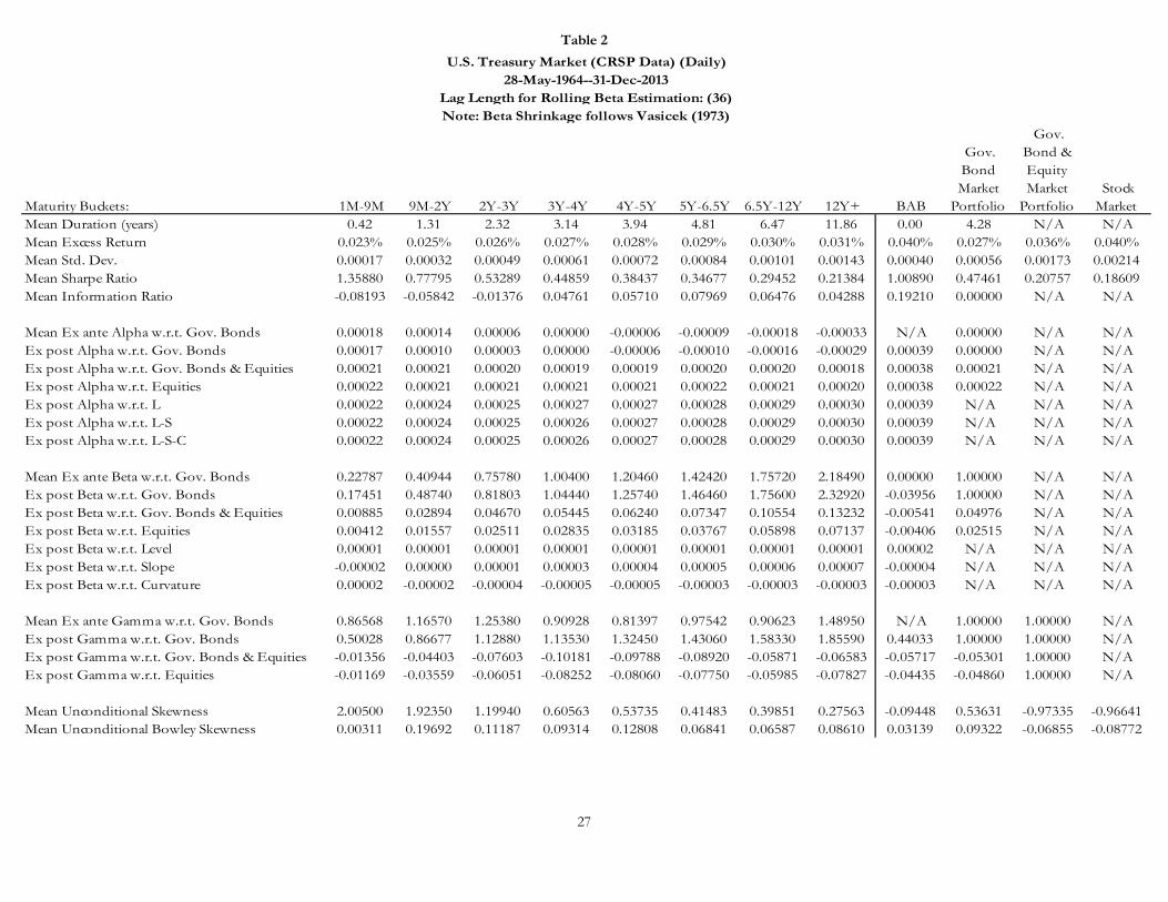
27  

Table 2

Maturity Buckets: 1M-9M 9M-2Y 2Y-3Y 3Y-4Y 4Y-5Y 5Y-6.5Y 6.5Y-12Y 12Y+ BAB

Gov. Bond Market

Portfolio

Gov. Bond & Equity Market

Portfolio Stock Market

Mean Duration (years) 0.42 1.31 2.32 3.14 3.94 4.81 6.47 11.86 0.00 4.28 N/A N/AMean Excess Return 0.023% 0.025% 0.026% 0.027% 0.028% 0.029% 0.030% 0.031% 0.040% 0.027% 0.036% 0.040%Mean Std. Dev. 0.00017 0.00032 0.00049 0.00061 0.00072 0.00084 0.00101 0.00143 0.00040 0.00056 0.00173 0.00214Mean Sharpe Ratio 1.35880 0.77795 0.53289 0.44859 0.38437 0.34677 0.29452 0.21384 1.00890 0.47461 0.20757 0.18609Mean Information Ratio -0.08193 -0.05842 -0.01376 0.04761 0.05710 0.07969 0.06476 0.04288 0.19210 0.00000 N/A N/A

Mean Ex ante Alpha w.r.t. Gov. Bonds 0.00018 0.00014 0.00006 0.00000 -0.00006 -0.00009 -0.00018 -0.00033 N/A 0.00000 N/A N/AEx post Alpha w.r.t. Gov. Bonds 0.00017 0.00010 0.00003 0.00000 -0.00006 -0.00010 -0.00016 -0.00029 0.00039 0.00000 N/A N/AEx post Alpha w.r.t. Gov. Bonds & Equities 0.00021 0.00021 0.00020 0.00019 0.00019 0.00020 0.00020 0.00018 0.00038 0.00021 N/A N/AEx post Alpha w.r.t. Equities 0.00022 0.00021 0.00021 0.00021 0.00021 0.00022 0.00021 0.00020 0.00038 0.00022 N/A N/AEx post Alpha w.r.t. L 0.00022 0.00024 0.00025 0.00027 0.00027 0.00028 0.00029 0.00030 0.00039 N/A N/A N/AEx post Alpha w.r.t. L-S 0.00022 0.00024 0.00025 0.00026 0.00027 0.00028 0.00029 0.00030 0.00039 N/A N/A N/AEx post Alpha w.r.t. L-S-C 0.00022 0.00024 0.00025 0.00026 0.00027 0.00028 0.00029 0.00030 0.00039 N/A N/A N/A

Mean Ex ante Beta w.r.t. Gov. Bonds 0.22787 0.40944 0.75780 1.00400 1.20460 1.42420 1.75720 2.18490 0.00000 1.00000 N/A N/AEx post Beta w.r.t. Gov. Bonds 0.17451 0.48740 0.81803 1.04440 1.25740 1.46460 1.75600 2.32920 -0.03956 1.00000 N/A N/AEx post Beta w.r.t. Gov. Bonds & Equities 0.00885 0.02894 0.04670 0.05445 0.06240 0.07347 0.10554 0.13232 -0.00541 0.04976 N/A N/AEx post Beta w.r.t. Equities 0.00412 0.01557 0.02511 0.02835 0.03185 0.03767 0.05898 0.07137 -0.00406 0.02515 N/A N/AEx post Beta w.r.t. Level 0.00001 0.00001 0.00001 0.00001 0.00001 0.00001 0.00001 0.00001 0.00002 N/A N/A N/AEx post Beta w.r.t. Slope -0.00002 0.00000 0.00001 0.00003 0.00004 0.00005 0.00006 0.00007 -0.00004 N/A N/A N/AEx post Beta w.r.t. Curvature 0.00002 -0.00002 -0.00004 -0.00005 -0.00005 -0.00003 -0.00003 -0.00003 -0.00003 N/A N/A N/A

Mean Ex ante Gamma w.r.t. Gov. Bonds 0.86568 1.16570 1.25380 0.90928 0.81397 0.97542 0.90623 1.48950 N/A 1.00000 1.00000 N/AEx post Gamma w.r.t. Gov. Bonds 0.50028 0.86677 1.12880 1.13530 1.32450 1.43060 1.58330 1.85590 0.44033 1.00000 1.00000 N/AEx post Gamma w.r.t. Gov. Bonds & Equities -0.01356 -0.04403 -0.07603 -0.10181 -0.09788 -0.08920 -0.05871 -0.06583 -0.05717 -0.05301 1.00000 N/AEx post Gamma w.r.t. Equities -0.01169 -0.03559 -0.06051 -0.08252 -0.08060 -0.07750 -0.05985 -0.07827 -0.04435 -0.04860 1.00000 N/A

Mean Unconditional Skewness 2.00500 1.92350 1.19940 0.60563 0.53735 0.41483 0.39851 0.27563 -0.09448 0.53631 -0.97335 -0.96641Mean Unconditional Bowley Skewness 0.00311 0.19692 0.11187 0.09314 0.12808 0.06841 0.06587 0.08610 0.03139 0.09322 -0.06855 -0.08772

U.S. Treasury Market (CRSP Data) (Daily)28-May-1964--31-Dec-2013

Lag Length for Rolling Beta Estimation: (36)Note: Beta Shrinkage follows Vasicek (1973)

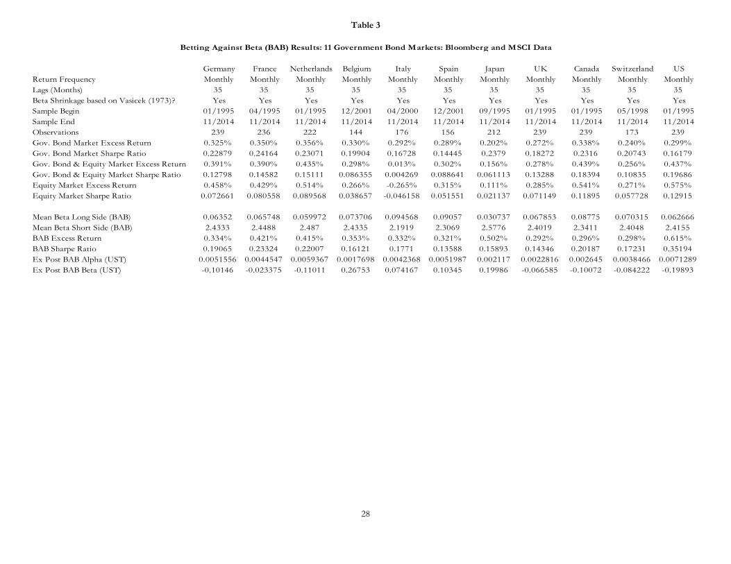
28  

Table 3

Germany France Netherlands Belgium Italy Spain Japan UK Canada Switzerland US

Return Frequency Monthly Monthly Monthly Monthly Monthly Monthly Monthly Monthly Monthly Monthly MonthlyLags (Months) 35 35 35 35 35 35 35 35 35 35 35Beta Shrinkage based on Vasicek (1973)? Yes Yes Yes Yes Yes Yes Yes Yes Yes Yes YesSample Begin 01/1995 04/1995 01/1995 12/2001 04/2000 12/2001 09/1995 01/1995 01/1995 05/1998 01/1995Sample End 11/2014 11/2014 11/2014 11/2014 11/2014 11/2014 11/2014 11/2014 11/2014 11/2014 11/2014Observations 239 236 222 144 176 156 212 239 239 173 239Gov. Bond Market Excess Return 0.325% 0.350% 0.356% 0.330% 0.292% 0.289% 0.202% 0.272% 0.338% 0.240% 0.299%Gov. Bond Market Sharpe Ratio 0.22879 0.24164 0.23071 0.19904 0.16728 0.14445 0.2379 0.18272 0.2316 0.20743 0.16179Gov. Bond & Equity Market Excess Return 0.391% 0.390% 0.435% 0.298% 0.013% 0.302% 0.156% 0.278% 0.439% 0.256% 0.437%Gov. Bond & Equity Market Sharpe Ratio 0.12798 0.14582 0.15111 0.086355 0.004269 0.088641 0.061113 0.13288 0.18394 0.10835 0.19686Equity Market Excess Return 0.458% 0.429% 0.514% 0.266% -0.265% 0.315% 0.111% 0.285% 0.541% 0.271% 0.575%Equity Market Sharpe Ratio 0.072661 0.080558 0.089568 0.038657 -0.046158 0.051551 0.021137 0.071149 0.11895 0.057728 0.12915

Mean Beta Long Side (BAB) 0.06352 0.065748 0.059972 0.073706 0.094568 0.09057 0.030737 0.067853 0.08775 0.070315 0.062666Mean Beta Short Side (BAB) 2.4333 2.4488 2.487 2.4335 2.1919 2.3069 2.5776 2.4019 2.3411 2.4048 2.4155BAB Excess Return 0.334% 0.421% 0.415% 0.353% 0.332% 0.321% 0.502% 0.292% 0.296% 0.298% 0.615%BAB Sharpe Ratio 0.19065 0.23324 0.22007 0.16121 0.1771 0.13588 0.15893 0.14346 0.20187 0.17231 0.35194Ex Post BAB Alpha (UST) 0.0051556 0.0044547 0.0059367 0.0017698 0.0042368 0.0051987 0.002117 0.0022816 0.002645 0.0038466 0.0071289Ex Post BAB Beta (UST) -0.10146 -0.023375 -0.11011 0.26753 0.074167 0.10345 0.19986 -0.066585 -0.10072 -0.084222 -0.19893

Betting Against Beta (BAB) Results: 11 Government Bond Markets: Bloomberg and MSCI Data

29  

Table 4

Return Frequency Daily Daily Monthly MonthlyLags (Months) 11 35 11 59Beta Shrinkage based on Vasicek (1973)? Yes Yes Yes YesSample Begin 05/1962 05/1964 05/1962 05/1966Sample End 12/2013 12/2013 12/2013 12/2013Observations 620 596 616 568Stock Market Sharpe Ratio 0.12249 0.18609 0.1133 0.19756Gov. Bond Market Sharpe Ratio 0.12668 0.20757 0.10838 0.21929BAB [F&P 2014] Sharpe Ratio 0.36728 1.0089 0.16216 0.97663

Unconstrained Mean Beta Long Side 0.32666 0.20096 0.15243 0.15495Mean Beta Short Side 2.1679 2.221 2.0624 2.1652Excess Return 0.018% 0.106% 0.504% 2.938%Sharpe Ratio 0.31779 1.2702 0.2833 1.2629Equity Beta Inequality Constraint (Gov. Bonds & Equities) Mean Beta Long Side 0.7089 0.58412 0.50434 0.49487Mean Beta Short Side 2.1679 2.221 2.0624 2.1652Excess Return 0.018% 0.101% 0.357% 2.374%Sharpe Ratio 0.38889 1.2224 0.27363 1.1763Equity Beta Inequality Constraint (Equities) Mean Beta Long Side 0.82717 0.67268 0.6961 0.56458Mean Beta Short Side 2.1679 2.221 2.0624 2.1652Excess Return 0.016% 0.088% 0.286% 2.323%Sharpe Ratio 0.35359 1.0917 0.25625 1.1529Slope Beta Equality Constraint Mean Beta Long Side 0.71046 0.73884 0.61251 0.66382Mean Beta Short Side 1.4282 1.3112 1.4111 1.3752Excess Return 0.006% 0.014% 0.049% 0.467%Sharpe Ratio 0.23055 0.42956 0.07557 0.54684Slope-Curvature Beta Equality Constraint Mean Beta Long Side 0.8625 0.87564 0.81768 0.84688Mean Beta Short Side 1.1596 1.0947 1.1009 1.1319Excess Return 0.005% 0.004% 0.101% 0.142%Sharpe Ratio 0.28829 0.22594 0.057628 0.36354Level-Slope-Curvature Beta Equality Constraint Mean Beta Long Side 0.90727 0.92986 0.89964 0.93943Mean Beta Short Side 1.0721 1.0299 1.0079 1.0334Excess Return 0.002% 0.002% 0.011% 0.038%Sharpe Ratio 0.22835 0.2114 0.058671 0.17551

BAB Unconstrained and Contrained Strategies: Covariance & PCsU.S. Treasury Market: CRSP Data

.

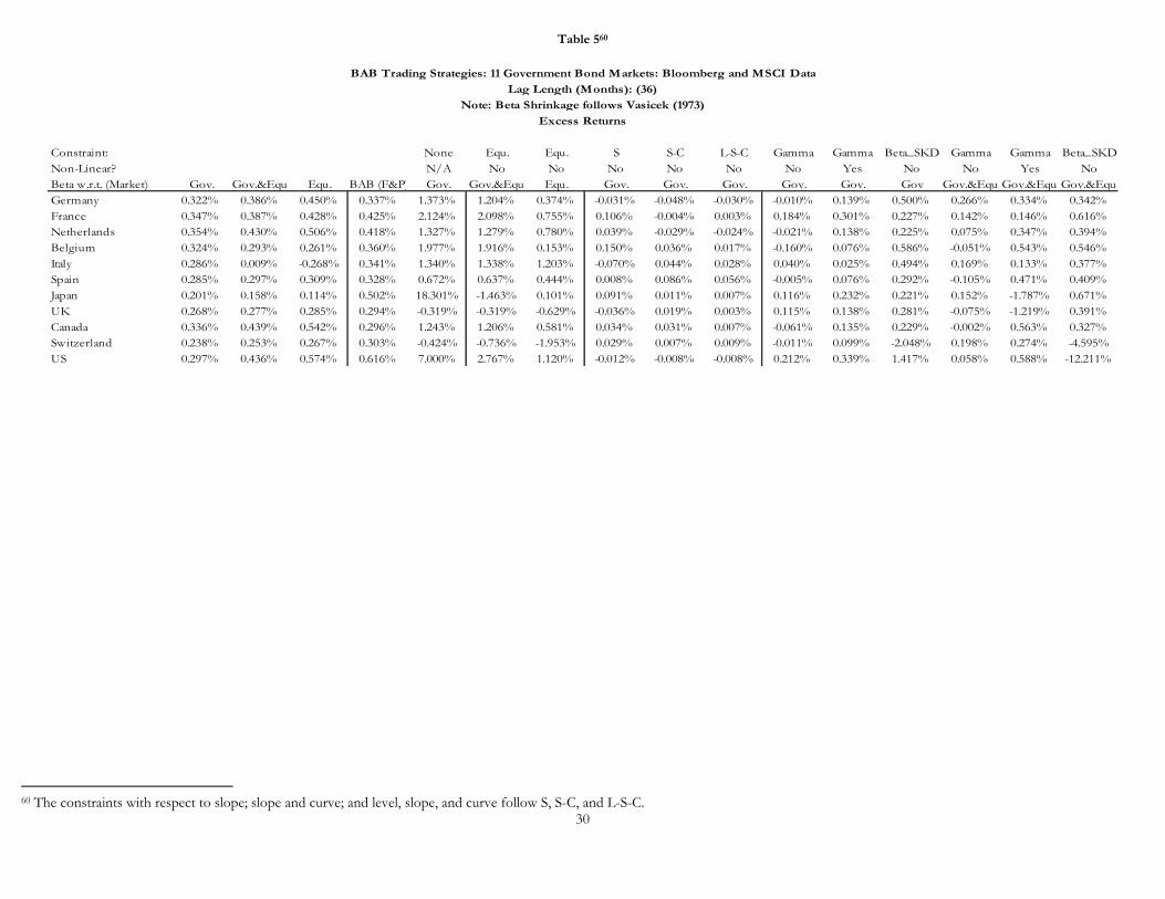
30  

Table 560

Constraint: None Equ. Equ. S S-C L-S-C Gamma Gamma Beta_SKD Gamma Gamma Beta_SKDNon-Linear? N/A No No No No No No Yes No No Yes NoBeta w.r.t. (Market) Gov. Gov.&Equ Equ. BAB (F&P) Gov. Gov.&Equ Equ. Gov. Gov. Gov. Gov. Gov. Gov Gov.&Equ Gov.&Equ Gov.&Equ.Germany 0.322% 0.386% 0.450% 0.337% 1.373% 1.204% 0.374% -0.031% -0.048% -0.030% -0.010% 0.139% 0.500% 0.266% 0.334% 0.342%France 0.347% 0.387% 0.428% 0.425% 2.124% 2.098% 0.755% 0.106% -0.004% 0.003% 0.184% 0.301% 0.227% 0.142% 0.146% 0.616%Netherlands 0.354% 0.430% 0.506% 0.418% 1.327% 1.279% 0.780% 0.039% -0.029% -0.024% -0.021% 0.138% 0.225% 0.075% 0.347% 0.394%Belgium 0.324% 0.293% 0.261% 0.360% 1.977% 1.916% 0.153% 0.150% 0.036% 0.017% -0.160% 0.076% 0.586% -0.051% 0.543% 0.546%Italy 0.286% 0.009% -0.268% 0.341% 1.340% 1.338% 1.203% -0.070% 0.044% 0.028% 0.040% 0.025% 0.494% 0.169% 0.133% 0.377%Spain 0.285% 0.297% 0.309% 0.328% 0.672% 0.637% 0.444% 0.008% 0.086% 0.056% -0.005% 0.076% 0.292% -0.105% 0.471% 0.409%Japan 0.201% 0.158% 0.114% 0.502% 18.301% -1.463% 0.101% 0.091% 0.011% 0.007% 0.116% 0.232% 0.221% 0.152% -1.787% 0.671%UK 0.268% 0.277% 0.285% 0.294% -0.319% -0.319% -0.629% -0.036% 0.019% 0.003% 0.115% 0.138% 0.281% -0.075% -1.219% 0.391%Canada 0.336% 0.439% 0.542% 0.296% 1.243% 1.206% 0.581% 0.034% 0.031% 0.007% -0.061% 0.135% 0.229% -0.002% 0.563% 0.327%Switzerland 0.238% 0.253% 0.267% 0.303% -0.424% -0.736% -1.953% 0.029% 0.007% 0.009% -0.011% 0.099% -2.048% 0.198% 0.274% -4.595%US 0.297% 0.436% 0.574% 0.616% 7.000% 2.767% 1.120% -0.012% -0.008% -0.008% 0.212% 0.339% 1.417% 0.058% 0.588% -12.211%

BAB Trading Strategies: 11 Government Bond Markets: Bloomberg and MSCI DataLag Length (Months): (36)

Note: Beta Shrinkage follows Vasicek (1973)Excess Returns

                                                            60 The constraints with respect to slope; slope and curve; and level, slope, and curve follow S, S-C, and L-S-C.

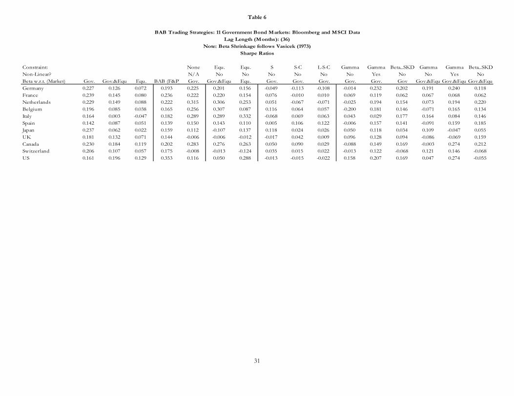
31  

Table 6

Constraint: None Equ. Equ. S S-C L-S-C Gamma Gamma Beta_SKD Gamma Gamma Beta_SKDNon-Linear? N/A No No No No No No Yes No No Yes NoBeta w.r.t. (Market) Gov. Gov.&Equ Equ. BAB (F&P) Gov. Gov.&Equ Equ. Gov. Gov. Gov. Gov. Gov. Gov Gov.&Equ Gov.&Equ Gov.&Equ.Germany 0.227 0.126 0.072 0.193 0.225 0.201 0.156 -0.049 -0.113 -0.108 -0.014 0.232 0.202 0.191 0.240 0.118France 0.239 0.145 0.080 0.236 0.222 0.220 0.154 0.076 -0.010 0.010 0.069 0.119 0.062 0.067 0.068 0.062Netherlands 0.229 0.149 0.088 0.222 0.315 0.306 0.253 0.051 -0.067 -0.071 -0.025 0.194 0.154 0.073 0.194 0.220Belgium 0.196 0.085 0.038 0.165 0.256 0.307 0.087 0.116 0.064 0.057 -0.200 0.181 0.146 -0.071 0.165 0.134Italy 0.164 0.003 -0.047 0.182 0.289 0.289 0.332 -0.068 0.069 0.063 0.043 0.029 0.177 0.164 0.084 0.146Spain 0.142 0.087 0.051 0.139 0.150 0.143 0.110 0.005 0.106 0.122 -0.006 0.157 0.141 -0.091 0.159 0.185Japan 0.237 0.062 0.022 0.159 0.112 -0.107 0.137 0.118 0.024 0.026 0.050 0.118 0.034 0.109 -0.047 0.055UK 0.181 0.132 0.071 0.144 -0.006 -0.006 -0.012 -0.017 0.042 0.009 0.096 0.128 0.094 -0.086 -0.069 0.159Canada 0.230 0.184 0.119 0.202 0.283 0.276 0.263 0.050 0.090 0.029 -0.088 0.149 0.169 -0.003 0.274 0.212Switzerland 0.206 0.107 0.057 0.175 -0.008 -0.013 -0.124 0.035 0.015 0.022 -0.013 0.122 -0.068 0.121 0.146 -0.068US 0.161 0.196 0.129 0.353 0.116 0.050 0.288 -0.013 -0.015 -0.022 0.158 0.207 0.169 0.047 0.274 -0.055

BAB Trading Strategies: 11 Government Bond Markets: Bloomberg and MSCI DataLag Length (Months): (36)

Note: Beta Shrinkage follows Vasicek (1973)Sharpe Ratios

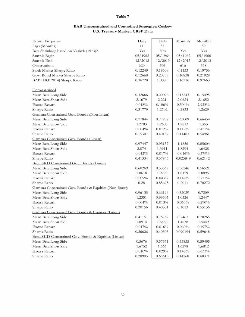
32  

Table 7

Return Frequency Daily Daily Monthly MonthlyLags (Months) 11 35 11 59Beta Shrinkage based on Vasicek (1973)? Yes Yes Yes YesSample Begin 05/1962 05/1964 05/1962 05/1966Sample End 12/2013 12/2013 12/2013 12/2013Observations 620 596 616 568Stock Market Sharpe Ratio 0.12249 0.18609 0.1133 0.19756Gov. Bond Market Sharpe Ratio 0.12668 0.20757 0.10838 0.21929BAB [F&P 2014] Sharpe Ratio 0.36728 1.0089 0.16216 0.97663

Unconstrained Mean Beta Long Side 0.32666 0.20096 0.15243 0.15495Mean Beta Short Side 2.1679 2.221 2.0624 2.1652Excess Return 0.018% 0.106% 0.504% 2.938%Sharpe Ratio 0.31779 1.2702 0.2833 1.2629Gamma Constrained Gov. Bonds (Non-linear) Mean Beta Long Side 0.77844 0.77932 0.63009 0.66454Mean Beta Short Side 1.2783 1.2605 1.2813 1.355Excess Return 0.004% 0.012% 0.112% 0.455%Sharpe Ratio 0.15307 0.40187 0.11483 0.54961Gamma Constrained Gov. Bonds (Linear) Mean Beta Long Side 0.97447 0.93137 1.1856 0.85604Mean Beta Short Side 2.074 1.3911 1.8294 1.6428Excess Return 0.012% 0.017% -0.016% 0.579%Sharpe Ratio 0.41334 0.57945 -0.025849 0.62142Beta_SKD Constrained Gov. Bonds (Linear) Mean Beta Long Side 0.60269 0.53567 0.56246 0.56521Mean Beta Short Side 1.8618 1.9299 1.8129 1.8895Excess Return 0.009% 0.043% 0.142% 0.777%Sharpe Ratio 0.28 0.85695 0.2011 0.70272Gamma Constrained Gov. Bonds & Equities (Non-linear) Mean Beta Long Side 0.96135 0.66194 0.52029 0.7209Mean Beta Short Side 1.2351 0.99605 1.0526 1.2447Excess Return 0.004% 0.013% 0.063% 0.290%Sharpe Ratio 0.20156 0.40301 0.1013 0.55156Gamma Constrained Gov. Bonds & Equities (Linear) Mean Beta Long Side 0.41151 0.76767 0.7467 0.70265Mean Beta Short Side 1.8914 1.5556 1.4638 1.5449Excess Return 0.017% 0.016% 0.060% 0.497%Sharpe Ratio 0.36626 0.40505 0.090194 0.59648Beta_SKD Constrained Gov. Bonds & Equities (Linear) Mean Beta Long Side 0.5676 0.57371 0.55835 0.59495Mean Beta Short Side 1.6752 1.666 1.6278 1.6812Excess Return 0.010% 0.029% 0.148% 0.633%Sharpe Ratio 0.28905 0.65618 0.14268 0.68371

BAB Unconstrained and Contrained Strategies: CoskewU.S. Treasury Market: CRSP Data

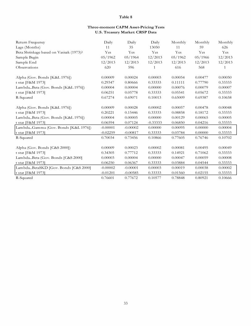
33  

Table 8

Return Frequency Daily Daily Daily Monthly Monthly MonthlyLags (Months) 11 35 13050 11 59 626Beta Shrinkage based on Vasicek (1973)? Yes Yes Yes Yes Yes YesSample Begin 05/1962 05/1964 12/2013 05/1962 05/1966 12/2013Sample End 12/2013 12/2013 12/2013 12/2013 12/2013 12/2013Observations 620 596 1 616 568 1

Alpha (Gov. Bonds [K&L 1976]) 0.00009 0.00024 0.00003 0.00054 0.00477 0.00050t stat [F&M 1973] 0.29347 0.80666 0.33333 0.11111 0.77790 0.33333Lambda_Beta (Gov. Bonds [K&L 1976]) 0.00004 0.00004 0.00000 0.00076 0.00079 0.00007t stat [F&M 1973] 0.06251 0.05778 0.33333 0.05541 0.05672 0.33333R-Squared 0.67274 0.69071 0.10013 0.65009 0.69387 0.10658

Alpha (Gov. Bonds [K&L 1976]) 0.00009 0.00028 0.00002 0.00057 0.00478 0.00048t stat [F&M 1973] 0.20221 0.15446 0.33333 0.08858 0.18172 0.33333Lambda_Beta (Gov. Bonds [K&L 1976]) 0.00004 0.00005 0.00000 0.00129 0.00065 0.00005t stat [F&M 1973] 0.06594 0.07124 -0.33333 0.06850 0.04216 0.33333Lambda_Gamma (Gov. Bonds [K&L 1976]) -0.00001 -0.00002 0.00000 0.00095 0.00000 0.00004t stat [F&M 1973] -0.02259 -0.00817 0.33333 0.03784 0.00000 0.33333R-Squared 0.70034 0.73456 0.10866 0.77605 0.76746 0.10702

Alpha (Gov. Bonds [C&S 2000]) 0.00009 0.00023 0.00002 0.00081 0.00495 0.00049t stat [F&M 1973] 0.34305 0.77712 0.33333 0.14921 0.71062 0.33333Lambda_Beta (Gov. Bonds [C&S 2000] 0.00003 0.00004 0.00000 0.00047 0.00059 0.00008t stat [F&M 1973] 0.06250 0.06367 0.33333 0.03884 0.04544 0.33333Lambda_BetaSKD [Gov. Bonds [C&S 2000] -0.00002 -0.00001 0.00003 0.00019 0.00038 0.00002t stat [F&M 1973] -0.01201 -0.00585 0.33333 0.01560 0.02155 0.33333R-Squared 0.76601 0.77672 0.10577 0.78848 0.80921 0.10666

Three-moment CAPM Asset-Pricing TestsU.S. Treasury Market: CRSP Data

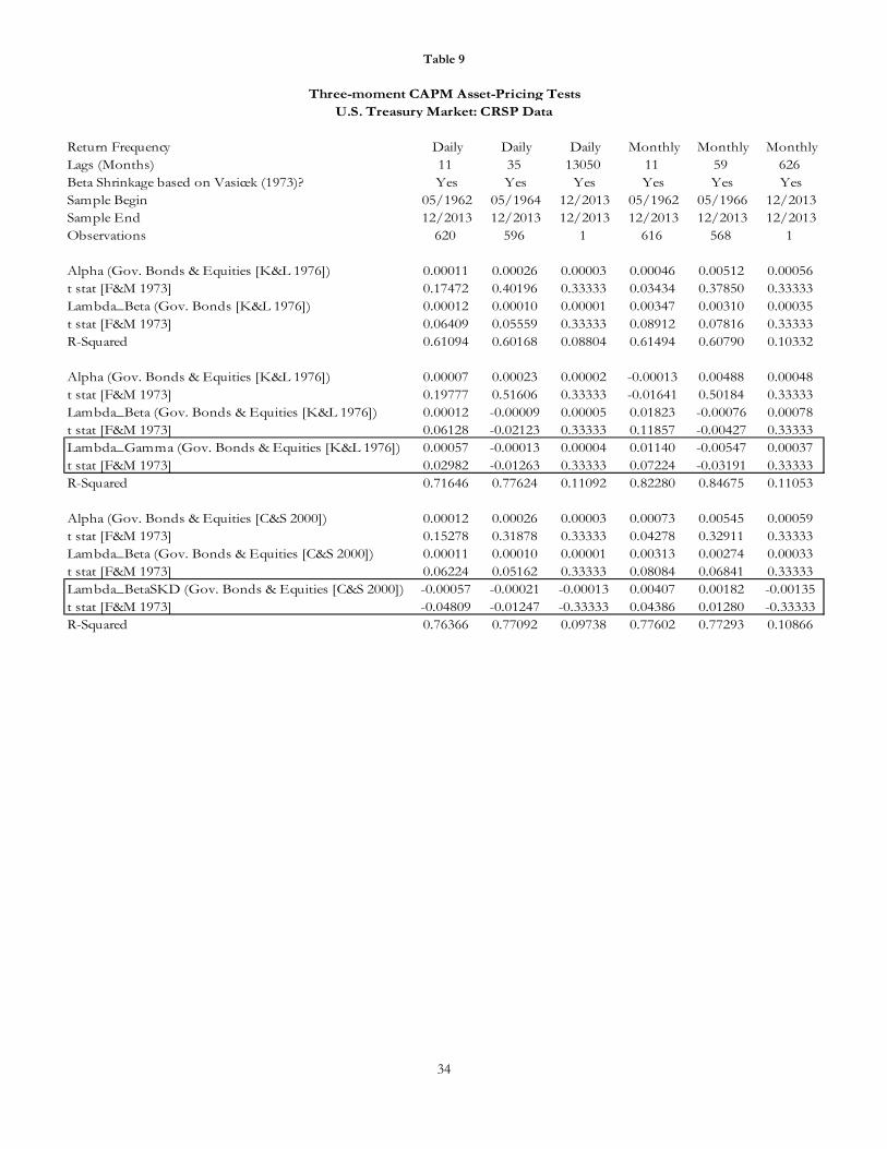
34  

Table 9

Return Frequency Daily Daily Daily Monthly Monthly MonthlyLags (Months) 11 35 13050 11 59 626Beta Shrinkage based on Vasicek (1973)? Yes Yes Yes Yes Yes YesSample Begin 05/1962 05/1964 12/2013 05/1962 05/1966 12/2013Sample End 12/2013 12/2013 12/2013 12/2013 12/2013 12/2013Observations 620 596 1 616 568 1

Alpha (Gov. Bonds & Equities [K&L 1976]) 0.00011 0.00026 0.00003 0.00046 0.00512 0.00056t stat [F&M 1973] 0.17472 0.40196 0.33333 0.03434 0.37850 0.33333Lambda_Beta (Gov. Bonds [K&L 1976]) 0.00012 0.00010 0.00001 0.00347 0.00310 0.00035t stat [F&M 1973] 0.06409 0.05559 0.33333 0.08912 0.07816 0.33333R-Squared 0.61094 0.60168 0.08804 0.61494 0.60790 0.10332

Alpha (Gov. Bonds & Equities [K&L 1976]) 0.00007 0.00023 0.00002 -0.00013 0.00488 0.00048t stat [F&M 1973] 0.19777 0.51606 0.33333 -0.01641 0.50184 0.33333Lambda_Beta (Gov. Bonds & Equities [K&L 1976]) 0.00012 -0.00009 0.00005 0.01823 -0.00076 0.00078t stat [F&M 1973] 0.06128 -0.02123 0.33333 0.11857 -0.00427 0.33333Lambda_Gamma (Gov. Bonds & Equities [K&L 1976]) 0.00057 -0.00013 0.00004 0.01140 -0.00547 0.00037t stat [F&M 1973] 0.02982 -0.01263 0.33333 0.07224 -0.03191 0.33333R-Squared 0.71646 0.77624 0.11092 0.82280 0.84675 0.11053

Alpha (Gov. Bonds & Equities [C&S 2000]) 0.00012 0.00026 0.00003 0.00073 0.00545 0.00059t stat [F&M 1973] 0.15278 0.31878 0.33333 0.04278 0.32911 0.33333Lambda_Beta (Gov. Bonds & Equities [C&S 2000]) 0.00011 0.00010 0.00001 0.00313 0.00274 0.00033t stat [F&M 1973] 0.06224 0.05162 0.33333 0.08084 0.06841 0.33333Lambda_BetaSKD (Gov. Bonds & Equities [C&S 2000]) -0.00057 -0.00021 -0.00013 0.00407 0.00182 -0.00135t stat [F&M 1973] -0.04809 -0.01247 -0.33333 0.04386 0.01280 -0.33333R-Squared 0.76366 0.77092 0.09738 0.77602 0.77293 0.10866

Three-moment CAPM Asset-Pricing TestsU.S. Treasury Market: CRSP Data

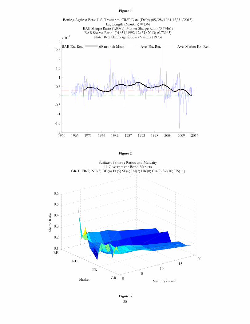
35  

Figure 1

Figure 2

Figure 3

1960 1965 1971 1976 1982 1987 1993 1998 2004 2009 2015-2

-1.5

-1

-0.5

0

0.5

1

1.5

2

2.5

3x 10

-3

Betting Against Beta: U.S. Treasuries: CRSP Data (Daily) (05/28/1964-12/31/2013)Lag Length (Months) = (36)

BAB Sharpe Ratio (1.0089), Market Sharpe Ratio (0.47461)BAB Sharpe Ratio: (01/31/1992-12/31/2013) (0.73965)

Note: Beta Shrinkage follows Vasicek (1973)

BAB Ex. Ret. 60-month Mean Ave. Ex. Ret. Ave. Market Ex. Ret.

05

1015

20

GR

FR

NE

BE0.1

0.2

0.3

0.4

0.5

0.6

Maturity (years)

Surface of Sharpe Ratios and Maturity11 Government Bond Markets

GR(1) FR(2) NE(3) BE(4) IT(5) SP(6) JN(7) UK(8) CA(9) SZ(10) US(11)

Market

Shar

pe R

atio

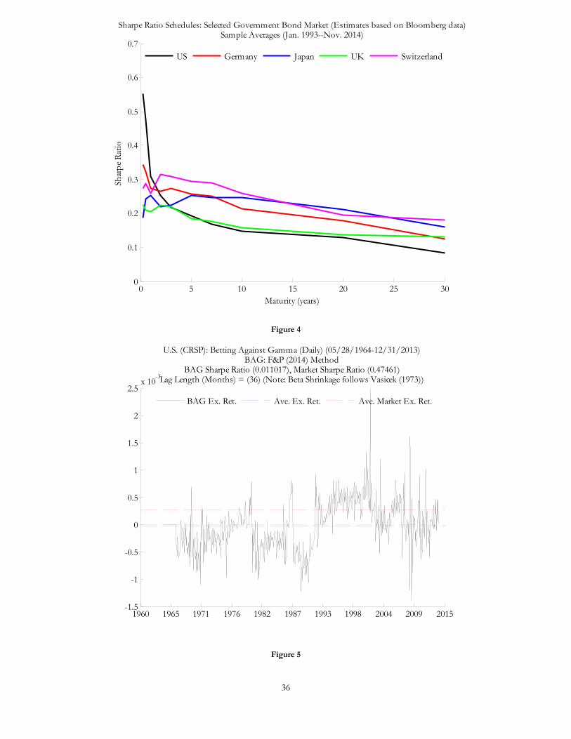
36  

Figure 4

Figure 5

0 5 10 15 20 25 300

0.1

0.2

0.3

0.4

0.5

0.6

0.7

Sharpe Ratio Schedules: Selected Government Bond Market (Estimates based on Bloomberg data)Sample Averages (Jan. 1993--Nov. 2014)

Maturity (years)

Shar

pe R

atio

US Germany Japan UK Switzerland

1960 1965 1971 1976 1982 1987 1993 1998 2004 2009 2015-1.5

-1

-0.5

0

0.5

1

1.5

2

2.5x 10

-3

U.S. (CRSP): Betting Against Gamma (Daily) (05/28/1964-12/31/2013)BAG: F&P (2014) Method

BAG Sharpe Ratio (0.011017), Market Sharpe Ratio (0.47461)Lag Length (Months) = (36) (Note: Beta Shrinkage follows Vasicek (1973))

BAG Ex. Ret. Ave. Ex. Ret. Ave. Market Ex. Ret.

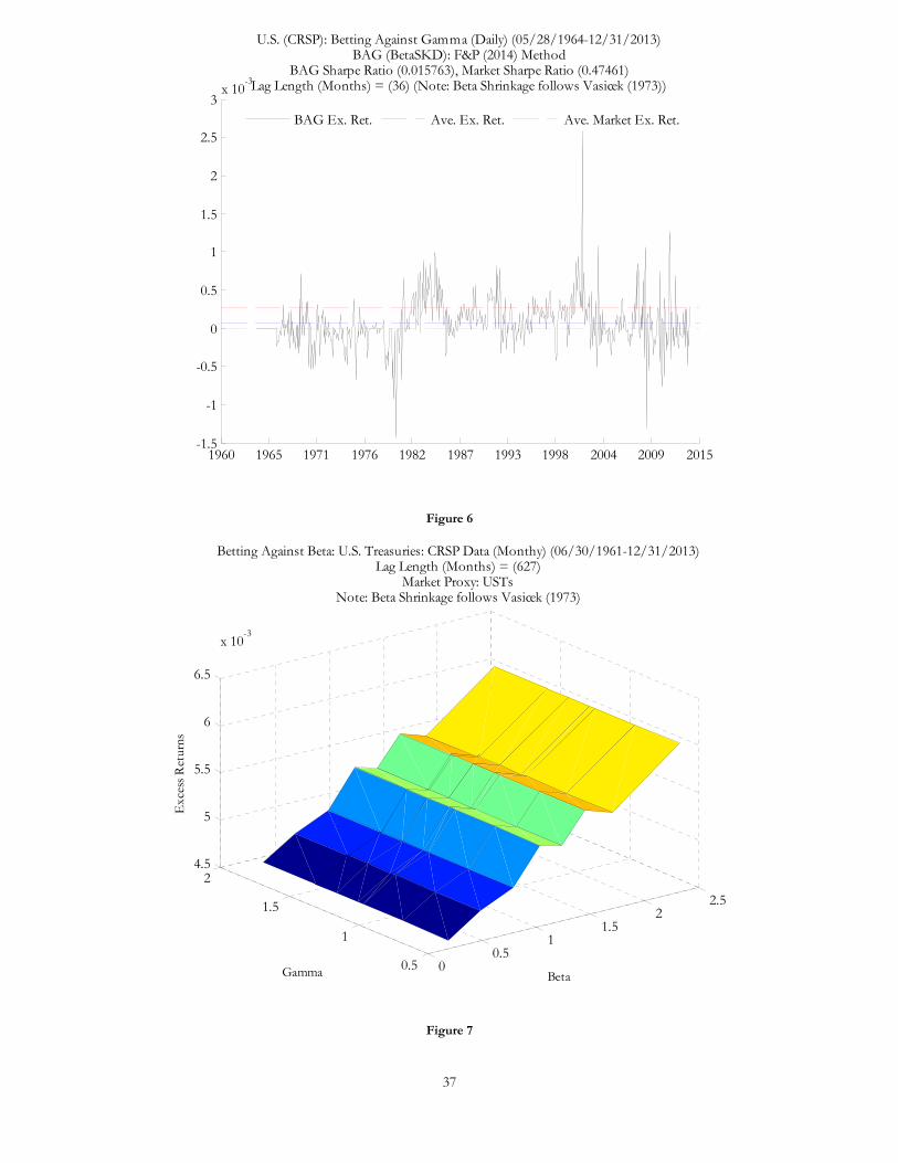
37  

Figure 6

Figure 7

1960 1965 1971 1976 1982 1987 1993 1998 2004 2009 2015-1.5

-1

-0.5

0

0.5

1

1.5

2

2.5

3x 10

-3

U.S. (CRSP): Betting Against Gamma (Daily) (05/28/1964-12/31/2013)BAG (BetaSKD): F&P (2014) Method

BAG Sharpe Ratio (0.015763), Market Sharpe Ratio (0.47461)Lag Length (Months) = (36) (Note: Beta Shrinkage follows Vasicek (1973))

BAG Ex. Ret. Ave. Ex. Ret. Ave. Market Ex. Ret.

00.5

11.5

22.5

0.5

1

1.5

24.5

5

5.5

6

6.5

x 10-3

Beta

Betting Against Beta: U.S. Treasuries: CRSP Data (Monthy) (06/30/1961-12/31/2013)Lag Length (Months) = (627)

Market Proxy: USTsNote: Beta Shrinkage follows Vasicek (1973)

Gamma

Exc

ess

Ret

urns

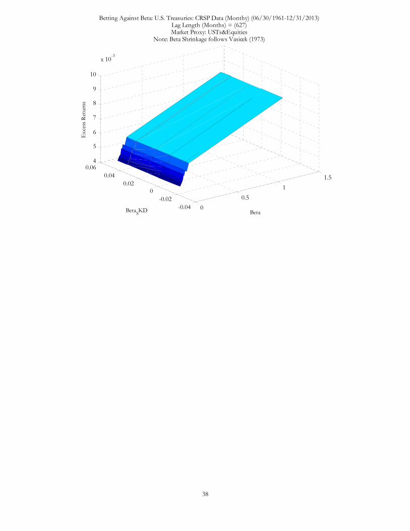
38  

0

0.5

1

1.5

-0.04-0.02

00.02

0.040.06

4

5

6

7

8

9

10

x 10-3

Beta

Betting Against Beta: U.S. Treasuries: CRSP Data (Monthy) (06/30/1961-12/31/2013)Lag Length (Months) = (627)Market Proxy: USTs&Equities

Note: Beta Shrinkage follows Vasicek (1973)

BetaSKD

Exc

ess

Ret

urns

39  

Appendix 1: GATSM-implied Sharpe Ratios

Although Duffee (2010) finds, notably empirically, an inverse relation SRs and maturity, that relation need not be so analytically. Consider a rudimentary, single-factor, short-rate affine model framework with

, expP r A Br (16)

where A and B are functions of maturity, , and r is the observed instantaneous short rate. Now define the Sharpe ratio (informally) as the expected excess return, or the (zero-coupon) term premium, scaled by the standard deviation of returns, as in

0

1 1sA Br E r ds

SRdP

VARP

(17)

To examine a tractable expression for the SR, under the Merton model, the short rate follows dr dt dW , and therefore

0

1 1

2sE r ds r (18)

Also, following Ito’s lemma,

22

2

12

P P P Pdt dWr rdP rP P P

(19)

And thus under the affine solution, namely with P

PBr

, the second term the captures the standard

deviation of returns, as in

dPVAR B

P (20)

Given the solution to the Merton model,61 the expression for the Sharpe ratio (SR) follows

2

2 31 1 12 6 2

1 1

2 6

r r

SR

(21)

                                                            61 See, say, Baz and Chacko (2004), pg. 136.

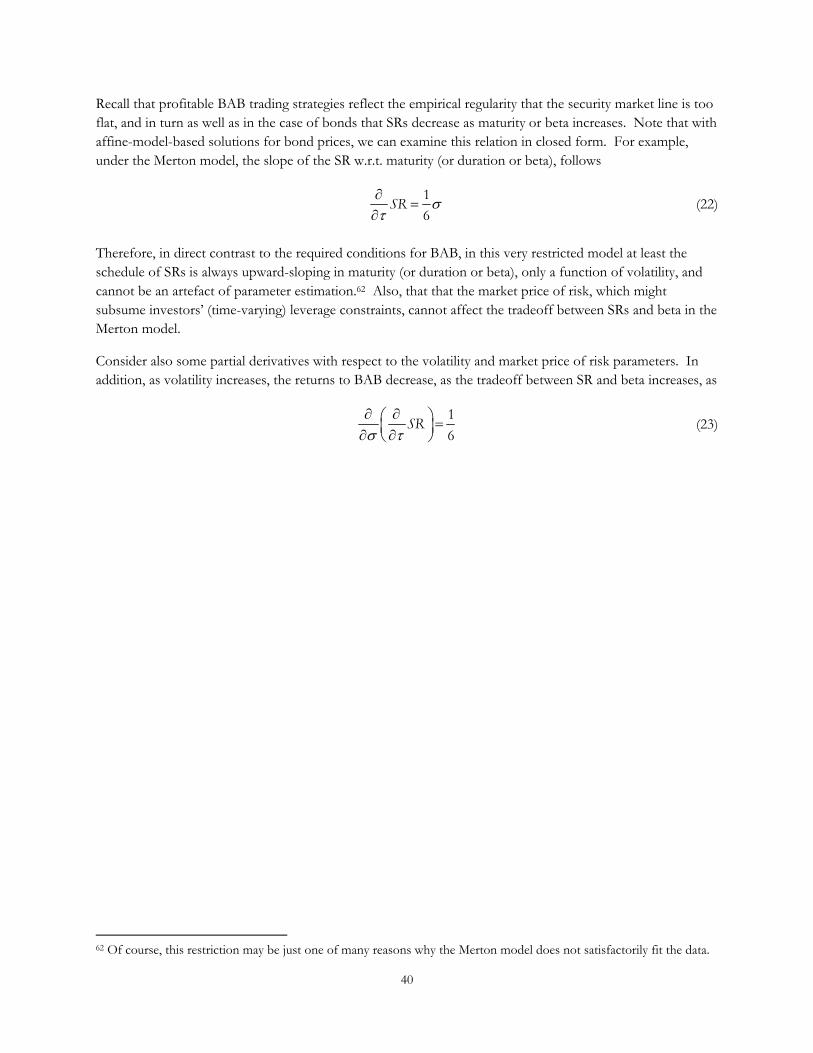
40  

Recall that profitable BAB trading strategies reflect the empirical regularity that the security market line is too flat, and in turn as well as in the case of bonds that SRs decrease as maturity or beta increases. Note that with affine-model-based solutions for bond prices, we can examine this relation in closed form. For example, under the Merton model, the slope of the SR w.r.t. maturity (or duration or beta), follows

1

6SR (22)

Therefore, in direct contrast to the required conditions for BAB, in this very restricted model at least the schedule of SRs is always upward-sloping in maturity (or duration or beta), only a function of volatility, and cannot be an artefact of parameter estimation.62 Also, that that the market price of risk, which might subsume investors’ (time-varying) leverage constraints, cannot affect the tradeoff between SRs and beta in the Merton model.

Consider also some partial derivatives with respect to the volatility and market price of risk parameters. In addition, as volatility increases, the returns to BAB decrease, as the tradeoff between SR and beta increases, as

1

6SR (23)

                                                            62 Of course, this restriction may be just one of many reasons why the Merton model does not satisfactorily fit the data.

41  

Appendix 2: Some Rudiments of Skew and Coskew Measures

Similar to the beta, , of an asset and portfolio variance, the gamma of an asset, , is the scaled marginal contribution to portfolio skew, with w is weight of asset i in the portfolio following

33

3

2

2

2 2

3

3

3cov 3

m m i i i ii ii i

i i iii

i i i i ii

m m i i

i m m m m i i

E r E w r ww w

E w rw

E w r r

E r r

r r E r E r

(24)

Given that 0i iE r , and scaling by 3

1

3 m mE r to ensure that market co-skew equals one, follows

2

3

cov i m m

i

m m

r r

E r

(25)

Note also the and can be derived from the coefficients in the following regression (and taking expectations), as in

2

, 0 1 , 2 ,

2

, 0 1 2 , 0

i t i i m t i m t m i

i t i i m i m t m

r c c r c r e

E r c c c E r

(26)

Taking differences and multiplying through by ,m t mr follows

2 2

, , , , 1 , 2 , ,

2 3 2

1 , 2 , , ,

m t m i t i t m t m i m t m i m t m m t m

i m t m i m t m m t m m t m

r r E r r c r c r E r

c r c r r E r

(27)

Again, taking expectations and noting that ,m t mE r , as in 

42  

2 3 2

, , , 1 , 2 , , ,

32 2

1 , 2 , ,0

m t m i t i t i m t m i m t m m t m m t m

i m t m i m t m m t m

E r r E r c E r c E r r E r

c E r c E r E r

(28)

Therefore

2 31 2

3

1 2 2

cov ,m m

m

m

m i i r i r

ri i i

r

r r c c

c c

(29)

For , multiplying through by 2

,m t mr , and again taking expectations leads to

2 3 4 2 2

, , , 1 , 2 , , ,

4 2 22 31 2 2 , , ,cov , r

m

m t m i t i t i m t m i m t m m t m m t m

i m i r i i m t m m t m m t m

E r r E r c E r c E r r E r

r c c c E r E r E r

(30)

And therefore,

4 4

1 2 3m m

m

r ri i i

r

c c

(31)

In addition to , a second measure of co-skew, follows Harvey and Siddique (2000, pg. 1276), as in

2, 1 , 1

2, 1 , 1

ˆi

i t M t

SKD

i t M t

E

E E

(32)

where , 1 , 1 , 1i t i t i i M tr r , i.e., the residual of the regression of excess return on the

contemporaneous market return.

Finally, Bowley skew, SB, follows

0.75 0.25 2 50

0.75 0.25B

P P PS

P P

(33)

where P is the th sample quantile.