Better Safe than Sorry?

Ex Ante and Ex Post Moral Hazard in Dynamic

Insurance Data∗

Jaap H. Abbring† Pierre-Andre Chiappori‡ Tibor Zavadil§

September 2008

Abstract

This paper empirically analyzes moral hazard in car insurance using a dynamic

theory of an insuree’s dynamic risk (ex ante moral hazard) and claim (ex post

moral hazard) choices and Dutch longitudinal micro data. We use the theory to

characterize the heterogeneous dynamic changes in incentives to avoid claims that

are generated by the Dutch experience-rating scheme, and their effects on claim

times and sizes under moral hazard. We develop tests that exploit these structural

∗We are grateful to Gerard van Rooijen and, in particular, Sander Tolk for patiently explaining thedata and the institutions to us. We also thank seminar participants at Columbia University, TinbergenInstitute, and Northwestern University; and participants in the Society for Economic Dynamics AnnualMeeting (Prague, June 2007), the Latin-American Meeting of the Econometric Society (Bogota, October2007), the Latin-American Economic Theory Meeting (Medellın, October 2007), the Third TinbergenInstitute Conference (Amsterdam, May 2008), and the Cowles Conference on Methods and Policy Appli-cations in Structural Microeconomics (New Haven, June 2008) for helpful discussion. Zavadil’s researchwas financially supported by the Netherlands Organisation for Scientific Research (NWO) through MaGWFree Competition grant 400-03-257.†CentER, Department of Econometrics & OR, Tilburg University, P.O. Box 90153, 5000 LE Tilburg,

The Netherlands. E-mail: J.H.Abbring@uvt.nl.‡Department of Economics, Columbia University, 1009A International Affairs Building, Mail Code

3308, 420 West 118th Street, New York, NY 10027, USA. Email: pc2167@columbia.edu.§Department of Economics, VU University Amsterdam, De Boelelaan 1105, 1081 HV Amsterdam,

The Netherlands, and Tinbergen Institute. Email: Tibor.Zavadil@gmail.com.Keywords: insurance, moral hazard, selection, state dependence, event-history analysis.JEL-codes: D82, G22, C41, C14.

1

implications of moral hazard and experience rating. Unlike much of the earlier

literature, we find evidence of moral hazard.

1 Introduction

Four decades of theoretical research on asymmetric information have firmly established

its importance for insurance relations and competitive insurance markets. The practical

relevance of this research, and of the results on the efficiency of insurance markets and

the design of optimal contracts that it has produced, depends critically on the empirical

relevance of asymmetric information. A substantial and fast growing literature is now

assessing this relevance for a variety of markets, using microeconometric methods and

micro data on contracts and insurees. For some markets, notably car insurance, evidence

is surprisingly mixed and muted, often pointing to a lack of asymmetric information prob-

lems. Much of the literature, however, uses static theory and cross-sectional data, which

limits both its versatility in dealing with truly dynamic aspects of insurance markets,

such as experience rating, and variation in the data that can be turned into robust em-

pirical results. The empirical distinction between moral hazard and selection effects using

static methods has turned out to be particularly hard; as argued by Abbring, Chiappori,

Heckman, and Pinquet (2003), this is the standard econometric problem of distinguishing

causal and selection effects.

This paper instead analyzes moral hazard in car insurance using panel data on con-

tracts and claims provided by a Dutch insurance company. The analysis exploits some

remarkable properties of the Dutch experience-rating system. Specifically, we theoretically

analyze the Dutch scheme as a repeated contract between an insuree and an insurer, in

which each period’s interaction involves memory of the relationship’s past history. Using

control theory, we study the endogenous changes this structure induces in the incentives

agents face at each point in time. Under moral hazard, these changes, in turn, generate

specific patterns in the time profile of claim occurrences and sizes that we fully character-

ize; these patterns are specific in the sense that they would not appear under the null of no

moral hazard. Finally, we develop structural econometric tests based on this theory and

apply them to the Dutch micro data. The tests are flexibly parametric and nonparamet-

1

ric, and valid in the presence of unobserved heterogeneity of a general type. In contrast

to much of the earlier literature, we find evidence of moral hazard in car insurance.

We also discuss the empirical distinction between ex ante and ex post moral hazard. Ex

ante moral hazard entails that agents respond to changes in incentives by changing the risk

of losses. Ex post moral hazard concerns the effects of incentives on claiming actual losses.

The distinction between ex ante and ex post moral hazard is important because of their

different welfare consequences (e.g. Chiappori, 2001). Because an insurer’s administrative

data typically only contain data on claims, and not on losses, distinguishing between

ex ante and ex post moral hazard requires additional structural assumptions. Under a

reasonable set of such assumptions, we find that at least some of the detected moral

hazard is due to ex post moral hazard.

Our theoretical model specifies agent’s optimal dynamic savings, loss prevention ef-

fort, and claim choices under the experience-rating (bonus-malus) scheme in Dutch car

insurance. It produces predictions on the joint behavior of the claim occurrence, claim

size, and experience-rating processes, for given individual risk and other characteristics.

Ex ante moral hazard is captured by the endogenous loss prevention effort; ex post moral

hazard by the endogenous claim choice. Endogenous savings allow for self-insurance.

The model provides a characterization of the dynamic heterogeneous incentives to

avoid claims inherent to the Dutch experience-rating scheme, and their behavioral conse-

quences under moral hazard. In particular, incentives are defined as the loss in expected

discounted utility that would be incurred if a claim would be filed. We show how incentives

vary with the current bonus-malus state and contract time, and jump with each claim

because of its foreseeable effect on the future bonus-malus state. We present an algorithm

for numerically characterizing these effects and provide a quantitative analysis of incen-

tives. We restrict attention to computations under the null of no moral hazard. Because

claim rates are constant under the null, these computations are relatively straightforward.

Our tests for moral hazard build on these theoretical computations. We first focus on

2

the timing of claims. Under the null that there is no moral hazard, claim rates do not

vary with incentives; under moral hazard, on the other hand, claim rates are lower when

incentives are stronger. Our main test exploits the full model structure. It is a score

(Lagrange multiplier) test for the dependence of claim rates on incentives in a version of

the structural model that allows for flexible heterogeneity in risk. Because it only requires

the computation of incentives under the null, it is easy to implement using our algorithm.

We find strong evidence that claim rates decrease with incentives, and reject the null of

no moral hazard at all conventional levels.

In addition to this structural parametric test for moral hazard, we also present and

apply a range of nonparametric tests for state-dependence and contract-time effects on

claim rates, controlling for risk heterogeneity. Our theory implies that any such effects

must be due to moral hazard and, in this way, identifies the substantial problem of testing

for moral hazard with the classical statistical problem of distinguishing state dependence

and heterogeneity. This is a hard problem, but one that has been studied at length

in statistics and econometrics (Bates and Neyman, 1952, Heckman and Borjas, 1980,

Heckman, 1981). Our tests rely on this literature’s key insight that, without contract-

time and state dependence, the number of claims in a given period is a sufficient statistic

for the unobserved heterogeneity in the conditional distribution of claim times in that

period. Consequently, any signs of time or state dependence in subsamples with a given

number of claims in a period are evidence of moral hazard. Moreover, an implication of

the Dutch experience-rating system is that incentives may jump up or down at the time a

claim is filed, depending on the current bonus-malus state. Therefore, we not only test for

state dependence, but also for appropriate changes in its sign across bonus-malus states.

Even though the nonparametric tests have relatively little power with the type of rare

events found in insurance data (Abbring and Zavadil, 2008), they corroborate the results

from the structural test.

Our theory also attributes a moral-hazard interpretation to state-dependence and

3

contract-time effects on the sizes of claims. Under the assumption that ex ante moral

hazard only affects the occurrence, but not the size, of insured losses, the latter are infor-

mative on ex post moral hazard. We complement this analysis of ex post moral hazard

with data on claim withdrawals. Agents in our data set can withdraw a claim within six

months and avoid malus. Under some assumptions, which we spell out in detail, claim

withdrawals are observed manifestations of ex post moral hazard.

This paper contributes to a rich literature on asymmetric information in insurance

markets. The seminal work on moral hazard and adverse selection by Arrow (1963),

Pauly (1974, 1968), and Rothschild and Stiglitz (1976) showed that competitive insurance

markets may be inefficient if information is asymmetric. A vast theoretical literature

followed up on their key insights. Increasingly, attention has shifted from the development

of theory to the empirical analysis of its relevance (see, e.g., Chiappori, 2001, Chiappori

and Salanie, 2003, for reviews).1 Chiappori (2001) forwarded the idea to exploit the

rich variation that can be derived from dynamic theory and found in longitudinal data;

Abbring, Chiappori, Heckman, and Pinquet (2003) suggested that we base a test for

moral hazard on the dynamic variation in individual risk with the idiosyncratic variation

in incentives due to experience rating.

The empirical papers most closely related to ours are Abbring, Chiappori, and Pin-

quet (2003), Dionne et al. (2006), and Pinquet et al. (2007). Our analysis differs from

and extends these works in several ways. First, we precisely model the forward-looking

behavior of an agent in the actual institutional environment characterizing the insurance

market studied. We use this model to define and compute dynamic incentives and con-

struct a structural test that exploits these computations in detail. Secondly, we explicitly

1Car-insurance data were studied, among others, by Dionne and Vanasse (1992), Puelz and Snow(1994), Dionne and Doherty (1994), Chiappori and Salanie (1997), Dionne, Gourieroux, and Vanasse(1999), Richaudeau (1999), Chiappori and Salanie (2000), Dionne, Gourieroux, and Vanasse (2001), Ab-bring, Chiappori, and Pinquet (2003), Cohen (2005), Dionne, Dahchour, and Michaud (2006), Chiappori,Jullien, Salanie, and Salanie (2006), and Pinquet, Dionne, Vanasse, and Maurice (2007). Health and lifeinsurance data were analyzed by, for example, Holly, Gardiol, Domenighetti, and Bisig (1998), Chiappori,Durand, and Geoffard (1998), Cardon and Hendel (2001), Hendel and Lizzeri (2003), and Fang, Keane,and Silverman (2006). Finkelstein and Poterba (2002) studied annuities.

4

distinguish ex ante and ex post moral hazard, which requires a formal analysis of the claim

filing behavior. Finally, we model both claim occurrences and claim sizes. Together, this

allows us to confront a novel and precise set of dynamic implications for claim occurrences

and sizes under moral hazard to longitudinal data.

The remainder of the paper is organized as follows. Section 2 briefly discusses the

Dutch car-insurance market, with specific attention for the experience-rating scheme used.

It also introduces the data. Section 3 develops the theory. We use the theory to analyze the

dynamic incentives inherent to experience rating, and to derive the implications of moral

hazard for claim rate and size dynamics. Section 4 develops an econometric framework

for testing the effects of moral hazard from data on claim rates and sizes and presents

the empirical results. Section 5 concludes. Appendices A and B provide proofs and

computational details for Section 3. Appendix C provides additional information on the

data.

2 Institutional Background and Data

2.1 Experience Rating in Dutch Car Insurance

In 2006, the 16.3 million inhabitants of the Netherlands were driving 7.2 million private

cars.2 Because liability insurance is mandatory in the Netherlands, this comes with a

substantial demand for car insurance. In the same year, 74 insurance companies served this

demand.3 Even though these companies are supervised by the Dutch financial authorities,

they are to great extent free to set their premiums and contractual conditions. In doing

so, the Dutch insurance companies, united in the Dutch Association of Insurers, have to

great extent coordinated their experience-rating systems in car insurance.

Before 1982, car insurers employed a limited experience-rating scheme. This scheme

was commonly considered to be inadequate to price observed risk. In the early 1980s, six

2Source: Statistics Netherlands (www.cbs.nl).3Source: Dutch Association of Insurers (www.verzekeraars.nl).

5

of the market’s leading firms proposed a much finer bonus-malus (BM) system, based on

a large actuarial study (de Wit et al., 1982).4 Early 1982, this system was introduced

in Dutch car insurance in a coordinated way. After some early market turbulence, the

insurers by and large settled on similar bonus-malus schemes.

This paper uses data from one of the six companies that were leading the introduction

of the bonus-malus system in Dutch car insurance. During the data period, January

1, 1995–December 31, 2000, this company used the bonus-malus scheme given in Table

1. The premium discount depends on the insuree’s current bonus-malus class, which

is determined at each annual contract renewal date. Twenty bonus-malus classes are

distinguished, from 1 (highest premium) to 20 (lowest premium). Every new insuree

starts in class 2 and pays the corresponding premium. We will refer to this premium

as the base premium. After each claim-free year, an insuree advances one class, up to

class 20. Each claim at fault sets an insuree back into a lower class. The worst class is

1, and implies a surcharge to the base premium. This scheme is representative for the

bonus-malus schemes used in the Netherlands in this period.5 Consequently, throughout

this paper we assume that the drivers in our data set cannot escape Table 1’s bonus-malus

system by switching insurers.

The empirical analysis in this paper exploits that the incentives to avoid a claim jump

with each claim filed, and vary with contract time and across bonus-malus classes. To gain

some first insight in the differences in the “cost” of a claim to an insuree across different

4 Information on the development of the BM system in Dutch car insurance is scattered throughoutthe professional literature. de Wit et al. (1982) provides information on the actuarial research underlyingthe bonus-malus system, and some very early history. Assurantiemagazine (2004) provides more recenthistorical reflection.

5The scheme is similar to the one originally proposed by de Wit et al. (1982), extended with multiple(maximum-bonus) levels that offer good customers some protection against premium increases. Evidenceon the development of the bonus-malus system is sketchy— see Footnote 4— but strongly suggests thatthe sector actively coordinated on similar bonus-malus schemes in the course of the 1980s, before the startof our data period. Moreover, further major innovations to car insurance pricing were only introducedrecently, after the end of our data period. We also compared Table 1’s scheme to schemes currentlyoffered by Dutch insurers and found only minor differences. The maximum discount on premium rangesfrom 70% to 80% and the maximum surcharge is in the range of 15% to 30%. Some insurance companiesoffer also collective insurance with more advantageous bonus-malus schemes.

6

bonus-malus classes and different numbers of claims, we have computed the change in the

premium at the next renewal date with each claim in a contract year, for different bonus-

malus classes. Table 2 gives the percentage premium change after a claim-free contract

year, and the subsequent marginal percentage changes in the premium after each claim

in the contract year. For example, after a claim-free year in class 8, an insuree will be

upgraded to class 9 and pay 45% instead of 50% of the base premium. This amounts

to a 10% reduction in the premium. If she files one claim in the contract year, she will

instead be downgraded to class 4 and pay 80% of the base premium. This amounts to

a (80 − 45)/45 = 78% increase relative to the premium that would be paid without the

claim. A second claim would take her down further to class 1, and a premium equal to

120% of the base (a 50% increase relative to having one claim). A third claim would have

no further effect on the premium.

Clearly, unlike the French scheme studied by Abbring, Chiappori, and Pinquet (2003),

this scheme is not proportional. The premium increases after a first claim are largest

for those in the intermediate bonus-malus classes, and smallest for those in the top and

bottom classes. The marginal premium increases after a second or third claim, however,

are increasing nearly monotonically with the bonus-malus class, from 0% in the lowest

classes to 100–140% in class 20.6 This all suggests that incentives to avoid a claim jump

down after a first claim for insurees in low classes and jump up after a first claim for

insurees in high classes. In Section 3, we formally define incentives in a dynamic theoretical

setting and provide some numerical computations to formalize this intuition.

Finally, note that insurees are contractually obliged to claim all their insured losses as

soon as possible. However, the contract leaves them the option to withdraw their claims

within six months from the loss date. Withdrawn claims do not count as at-fault claims

in determining the insuree’s bonus-malus class and therefore do not affect the premium.

6In the lowest classes, therefore, the bonus-malus scheme itself does not give incentives to avoid asecond or third claim. However, the insurance company reserves the right to cancel contracts with threeor more claims at fault in a year. Because claims at fault are fairly rare, this is unlikely to affect insurees’decisions a lot. Therefore, we ignore contract cancelations in our theoretical and empirical analysis.

7

Therefore, throughout most of the paper we treat withdrawn claims like unclaimed losses.

That is, we ignore them, together with losses that were not claimed in the first place.

Section 4.4 discusses the fact that withdrawals are in fact observed manifestations of ex

post moral hazard.

2.2 Data

Our data provide the contract and claim histories of personal car insurance clients of a

major Dutch insurer from January 1, 1995 to December 31, 2000. The raw data consist

of 1,730,559 records. Each record registers a change in a particular contract (renewal,

change of car, etcetera), or a claim. The data include 75 variables, with information

on drivers (sex, age, occupation, postcode), cars (brand, model, production year, price,

weight, power, etc.), contracts (coverage, bonus-malus class, level of deductible, premium,

renewal date), and claims (type of claim, damage, etc.).

The raw data contains 163,194 unique contracts. Because they do not contain infor-

mation on claims in 1995, we excluded this year from the data. We also excluded the

contracts that are not covered by the bonus-malus system.7 This leaves 140,799 unique

contracts with a total of 101,074 claims. Of these claims, 34,491 are claims at fault that

may lead to a malus.8 However, in 2,463 of these cases, insurees have avoided a malus

by withdrawing their claim.9 Throughout most of the paper, we treat withdrawn claims

as unclaimed losses, and simply exclude them from the analysis. Section 4.4 specifically

studies the withdrawal data to learn about moral hazard. Appendix C shows that the

empirical results presented in the main text are robust to alternative ways of dealing with

withdrawals.

7These are the contracts covering companies’ fleets of cars. Such contracts have no individual BMcoefficients, but general fleet discounts. These discounts are adjusted every year based on the fleets’ claimhistories.

8The data also include so called “nil” claims, which are mostly pro forma claims of amounts belowthe deductible. These may correspond to an “at fault” event, but typically do not affect the agent’sbonus-malus status. Therefore, we treat all nil claims as claims not-at-fault.

9We use both direct and indirect information to identify withdrawals. See Appendix C for details.

8

We restrict our analysis to the claim histories from the contracts’ first renewal (or

start) date in the sample onwards. In the data, there are 124,021 contracts with observed

renewal date. Of these contracts, 6,787 were interrupted for some period of time. In these

cases, we only use the contract history from its first observed renewal date to its first

interruption.

For each contract, we registered the claim history, with information on the times and

sizes of claims at fault that were not withdrawn. We examined the bonus-malus transi-

tions between all observed contract years, corrected some inconsistencies (see Appendix

C for details), and registered the initial bonus-malus class (i.e., the bonus-malus class

established at the first renewal date). Along the way, we discovered that the data on the

bonus-malus class after the 2000 renewal are not reliable.10 Therefore, we excluded con-

tracts that started in 2000, and the history of ongoing contracts after their 2000 renewal

date.

Our full final sample consists of 123,169 unique contracts with 23,396 claims at fault.

Table 3 shows that many of these are observed for the maximum period of 4 years.

We illustrate some of the data’s key features using only data on the first fully observed

contract years in the sample. Table 4 gives the number of contracts in this subsample by

bonus-malus class and by number of claims at fault filed in the contract year. Contracts

with one claim and contracts with two or more claims will be important, for different

reasons, to our empirical analysis. There are a lot of contracts with one claim in our

subsample but, because claims are rare, there are only 278 contracts with at least two

claims.

Figure 1 plots the distribution of contracts in our subsample across bonus-malus

classes. Classes 1 – 3 have less than 1% of the contracts each; more than 26% of the

contracts are in the highest class 20. The majority of contracts (over 57%) is in the high

bonus-malus classes 14 – 20, where the premium is just 25% of the base premium.

1040,104 out of 68,515 bonus-malus transitions in 2000 were incorrect.

9

Figure 1 also plots the shares of contracts in our subsample with at least one and at

least two claims at fault, by bonus-malus class. These shares drop substantially with the

bonus-malus class. It may be tempting to relate this variation in the number of claims

over bonus-malus classes to our discussion of incentives. However, the overall pattern can

be well explained by heterogeneity in risk, with high-risk individuals sorted into the lower

bonus-malus classes.

3 Model of Claim Rates and Sizes

This section characterizes the dynamic incentives to avoid car insurance claims that are

inherent to the Dutch bonus-malus scheme. We do so by analyzing a model of a sin-

gle agent’s risk prevention and claim behavior that combines features of Mossin’s (1968)

static model of insurance and Merton’s (1971) continuous-time analysis of optimal con-

sumption. Our model is related to Briys (1986), but focuses on experience rating and

its moral-hazard effects. It is an extension of Abbring, Chiappori, and Pinquet’s (2003)

model with heterogeneous losses and endogenous claiming, carefully adapted to the Dutch

institutional environment. Also, unlike Abbring et al.’s analysis of experience rating in

French car insurance, we make the nonstationarity arising from annual premium revision

explicit. This is important for our empirical analysis because in the Dutch bonus-malus

system, unlike in the French one, both the number of past claims and their distribution

across contract years matter for the current bonus-malus status.

3.1 Primitives

We consider the behavior and outcomes of an agent i in continuous time τ with infinite

horizon. Time is measured in contract years and has its origin at the moment the agent

entered the insurance market.

The wealth of agent i at time τ is denoted by Wi(τ) and accumulates as follows. At

10

time 0, agent i is endowed with some initial wealth Wi(0) > 0. Then, between τ and

τ + dτ , agent i receives a return ρWi(τ)dτ on her wealth and consumes ci(τ)dτ . We

ignore any other income, such as labor income.11

The agent causes an accident between τ and τ + dτ with some probability pi(τ)dτ .12

If so, she incurs some monetary loss. Denote the j-th loss incurred by agent i by Lij.

We assume that Lij is drawn independently of the agent’s insurance history, including

(Li1, . . . , Li(j−1)), from some time-invariant distribution Fi.13 The losses Lij are covered

by an insurance contract involving a fixed deductible Di and a premium qi(τ)dτ that is

paid continuously. The deductible is applied on a claim-by-claim basis, i.e. if a claim for

a loss Lij is filed, the insurer pays Lij −Di to the agent.

The premium qi(τ) is determined by agent i’s bonus-malus class Ki(τ) according to

Table 1. Thus, we can write qi(τ) = Ai(Ki(τ)), where Ai is a mapping from agent

i’s bonus-malus class into her flow premium. Because the base premium to which the

discounts in Table 1 are applied depends on agent i’s characteristics, the mapping Ai will

be heterogeneous across agents.14

Agent i is endowed with an initial bonus-malus class Ki(0). The bonus-malus class is

updated at the beginning of each contract year, the renewal date, according to the rule

in Table 1. Thus, Ki(τ) is a right-continuous process, with discrete steps at each renewal

date τ ∈ N depending on the past contract year’s bonus-malus class and number of claims.

Denote by Ni(τ) the number of claims in the ongoing contract year up to and including

time τ . That is, Ni(τ) is a claim-counting process that is set to zero at the beginning of

11For the purpose of our analysis, this is equivalent to assuming that any such income is perfectlyforeseen by the agent (Merton, 1971, Section 7).

12Accidents that are not caused by the agent are fully covered and have no impact on future premiums.Such accidents can be and are disregarded in our analysis. From now on, by accident or claim we alwaysmean accident or claim at fault.

13This assumption is violated if agents can influence Fi ex ante by choosing to drive more or lesscarefully. Then, data on claim sizes do not distinguish between ex ante and ex post moral hazard, butare still informative on the overall presence of moral hazard.

14Here, we abstract from time-varying characteristics other than Ki. There is not much harm in treatinge.g. age as a time-invariant characteristic, as our empirical analysis will focus on events in only one or afew contract years.

11

each contract year. Then, at each renewal date τ ∈ N,

Ki(τ) = B(Ki(τ−), Ni(τ−)), (1)

where Ki(τ−) and Ni(τ−) are agent i’s bonus-malus class and number of claims in the

past contract year, respectively, and B represents Table 1’s bonus-malus updating rule.

Note that this rule is common to all agents. Recall that it moves agents who survive

a contract year without claims to a higher bonus-malus class, corresponding to a lower

premium, and all other agents to a lower class, with a higher premium.

Insurance claims filed by the agent are potentially affected by ex ante and ex post

moral hazard (Chiappori, 2001). Ex ante moral hazard arises if the agent can affect the

probability of an accident. We model this by allowing, at each time τ , the agent to choose

the intensity pi (τ) of having an accident from some bounded interval [pi, pi], at a utility

cost Γi (pi (τ)). We assume that Γi is twice differentiable on (pi, pi), with Γ′i < 0, Γ′′i > 0.

In words, reducing accident rates is costly and returns to prevention are decreasing. For

definiteness, we also assume that Γ′i(pi+) = −∞ and Γ′i(pi−) = 0. In addition, we allow

for ex post moral hazard by allowing the agent to hide a loss she has actually incurred

from the insurer. For clarity of exposition, we assume that claiming and hiding losses are

costless, but that the agent cannot claim losses that have not actually been incurred.15

The agent’s instantaneous utility from consuming ci(τ) and driving with accident in-

tensity pi(τ) at time τ is ui (ci (τ))−Γi (pi (τ)). We assume that ui is strictly increasing and

concave. The agent chooses consumption, prevention and claiming plans that maximize

total expected discounted utility16

E[∫ ∞

0

e−ρτ [ui (ci(τ))− Γi (pi(τ))] dτ

],

15Section 3.3.1 discusses a simple extension of the model in which hiding losses is costly. Such anextension is needed to formalize variation in the degree of ex post moral hazard in general, and theextreme case that agents report all losses (above the deductible) and do not suffer from ex post moralhazard in particular.

16For simplicity, we assume that subjective discount rates equal the interest rate.

12

subject to the intertemporal budget constraint limτ→∞ e−ρτW (τ) = 0 and given the wealth

and premium dynamics described above.

At each time τ , the agent observes her wealth, bonus-malus class and claim histories.

As we have implicitly assumed that any labor and other income is perfectly foreseen by

the agent, she only has to form expectations on future accidents and their implications.

3.2 Optimal Risk, Claims and Savings

For notational convenience, we now drop the index i. It should be clear, however, that

all results are valid at the individual level, irrespective of the distribution of preferences

and technologies across agents. In particular, the results hold for any type of unobserved

heterogeneity in these primitives of the model.

Because our model is Markovian and, apart from annual contract renewal, time-

homogeneous, the optimal consumption, prevention and claim decisions at time τ only

depend on the past history through the agent’s current wealth W (τ), bonus-malus class

K(τ), the number of claims at fault N(τ), and the time t ≡ τ − [τ ] past in the ongoing

contract year.

Let V (t,W,K,N) denote the agent’s optimal expected discounted utility at time t in

the contract year if her wealth equals W , she is in bonus-malus class K, and has claimed

N losses in the ongoing contract year. This value function satisfies the Bellman equation

V (t,W,K,N) =

maxc,p,X

{u(c)dt− Γ(p)dt+ e−ρdt×[(1− pdt)V (t+ dt, (1 + ρdt)W − cdt− A(K)dt,K,N)

+ pdt

∫XV (t+ dt, (1 + ρdt)W −min{l, D} − cdt− A(K)dt,K,N + 1)dF (l)

+ pdt

∫X c

V (t+ dt, (1 + ρdt)W − l − cdt− A(K)dt,K,N)dF (l)]},

(2)

13

with

V (1,W,K,N) ≡ limt↑1

V (t,W,K,N) = V (0,W,B(K,N), 0). (3)

Equation (2) can be interpreted as follows. Between t and t + dt the agent derives flows

of utility from her consumption and disutility from her prevention effort. The value

V (t,W,K,N) equals the net value of these utility flows, at the optimal consumption

and prevention levels, plus the expected optimal discounted utility at time t + dt. With

probability 1 − pdt no accident occurs. Then, the agent’s wealth is increased with the

interest flow minus consumption and the premium, and the number of claims at fault, N ,

stays unchanged. If the agent causes an accident, with probability pdt, she will incur an

additional wealth loss. The size of this wealth loss is subject to ex post moral hazard. If

the damage L caused by the accident lies in the optimal choice of the claim set X , she

claims for insurance compensation and only looses the minimum of L and the deductible

D. Then, the number of claims at fault, N , increases by 1. If L lies in the complement

X c of the optimal claim set, however, she does not claim and pays the full loss L. Then,

the number of claims at fault, N , stays unchanged.

Equation (3) reflects the effects of annual premium renewal. It requires that the value

in class K with N claims just before a renewal time equals the value in class B(K,N)

with 0 claims just after renewal.

Bellman equation (2) can be rewritten in a more familiar form by rearranging and

taking limits dt ↓ 0,

ρV (S) = maxc,p,X

{u(c)− Γ(p)

+ p[∫XV (t,W −min{l, D}, K,N + 1)dF (l)

+

∫X c

V (t,W − l,K,N)dF (l)− V (S)]

+ VW (S) [ρW − c− A(K)] + Vt(S)},

(4)

14

where Vt and VW are the partial derivatives of V with respect to, respectively, t and

W . The left-hand side of (4) is the flow (or perpetuity) value attached by the agent to

state S ≡ (t,W,K,N). It equals the (optimal) instantaneous flow of utility from her

consumption net of the disutility from her prevention effort plus three expected value

(“capital”) gains terms, (i) the expected value gain because of an accident, (ii) the value

gain due to net accumulation of wealth, and (iii) the appreciation of the value over time.

Standard arguments guarantee that (4), with (3), has a unique solution V , and that

an optimal consumption-prevention-claim plan exists. In Appendix A, we prove that the

value function V is strictly increasing in wealth W (Lemma 1) and that it is weakly

increasing in the bonus-malus class K and weakly decreasing in the number of claims at

fault N (Lemma 2).

One direct implication is that the agent follows a threshold rule for claiming.

Proposition 1. The optimal claim set in state S is given by X ∗(S) ≡ (x∗(S),∞), for

some claim threshold x∗(S) ≥ D.

Thus, if the agent incurs a loss L at time t then, for given wealth W , bonus-malus class

K and number of claims at fault N right before t, she claims if and only if L > x∗(S).

The threshold is implicitly defined as the loss at which she is indifferent between claiming

and not claiming:

V (t,W −D,K,N + 1) = V (t,W − x∗(S), K,N). (5)

This assumes an internal solution and, in particular, ignores the trivial, and empirically

irrelevant, case in which X = ∅.

Optimality of the two remaining choices, consumption and prevention, requires that

15

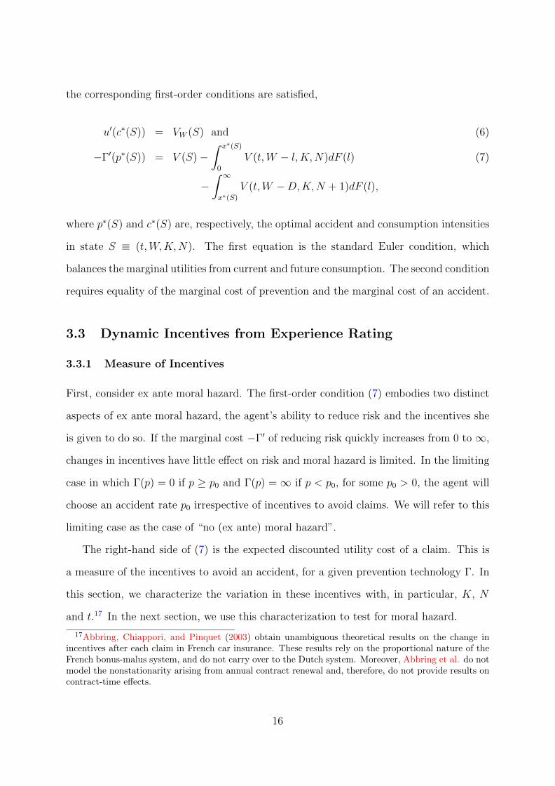
the corresponding first-order conditions are satisfied,

u′(c∗(S)) = VW (S) and (6)

−Γ′(p∗(S)) = V (S)−∫ x∗(S)

0

V (t,W − l,K,N)dF (l) (7)

−∫ ∞x∗(S)

V (t,W −D,K,N + 1)dF (l),

where p∗(S) and c∗(S) are, respectively, the optimal accident and consumption intensities

in state S ≡ (t,W,K,N). The first equation is the standard Euler condition, which

balances the marginal utilities from current and future consumption. The second condition

requires equality of the marginal cost of prevention and the marginal cost of an accident.

3.3 Dynamic Incentives from Experience Rating

3.3.1 Measure of Incentives

First, consider ex ante moral hazard. The first-order condition (7) embodies two distinct

aspects of ex ante moral hazard, the agent’s ability to reduce risk and the incentives she

is given to do so. If the marginal cost −Γ′ of reducing risk quickly increases from 0 to ∞,

changes in incentives have little effect on risk and moral hazard is limited. In the limiting

case in which Γ(p) = 0 if p ≥ p0 and Γ(p) =∞ if p < p0, for some p0 > 0, the agent will

choose an accident rate p0 irrespective of incentives to avoid claims. We will refer to this

limiting case as the case of “no (ex ante) moral hazard”.

The right-hand side of (7) is the expected discounted utility cost of a claim. This is

a measure of the incentives to avoid an accident, for a given prevention technology Γ. In

this section, we characterize the variation in these incentives with, in particular, K, N

and t.17 In the next section, we use this characterization to test for moral hazard.

17Abbring, Chiappori, and Pinquet (2003) obtain unambiguous theoretical results on the change inincentives after each claim in French car insurance. These results rely on the proportional nature of theFrench bonus-malus system, and do not carry over to the Dutch system. Moreover, Abbring et al. do notmodel the nonstationarity arising from annual contract renewal and, therefore, do not provide results oncontract-time effects.

16

We focus on the dynamic incentives inherent to the bonus-malus scheme and set the

deductible D to 0. This simplifies the presentation and does not greatly interfere with our

objective of learning about changes in incentives across states. Section 3.3.2 formalizes

this point in the context of a particular model specification.

We will also restrict attention to incentives in the case without moral hazard. This

will be sufficient for computing a score test for moral hazard and for interpreting local

behavior of econometric tests near the null of no moral hazard. Without moral hazard,

the optimal accident rate p∗(S) equals a fixed number p0 > 0 in all states S and all losses

are claimed, so the right-hand side of (7) simplifies to

V (t,W,K,N)− V (t,W,K,N + 1). (8)

We will characterize incentives in the case of no moral hazard by characterizing this

difference in utility values as a function of the state (t,W,K,N).

Before we move to these computations, note that (8) is also a measure of incentives

to avoid a claim given that an accident has occurred. Linearizing (5) as a function of the

threshold around the deductible D = 0 gives

x∗(t,W,K,N)VW (t,W,K,N) ≈ V (t,W,K,N)− V (t,W,K,N + 1). (9)

The right-hand side of this equation is again the expected discounted utility cost of a

claim in (8). The left-hand side is the marginal cost, in expected discounted utility

units and at a time a claim decision needs to be taken, of increasing the threshold just

above the deductible D = 0. Note that this cost, unlike the cost Γ of loss prevention,

is not a free parameter of the model. This is a direct consequence of our assumption

that claiming and hiding losses are costless, and implies that the model does not have

a parameter that indexes the degree of ex post moral hazard. It is straightforward to

extend the model with such a parameter. For example, if hiding a loss L leads to a

17

capital loss of γL, for some parameter γ ≥ 1, then the left-hand side of (9) generalizes

to γx∗(t,W,K,N)VW (t,W,K,N). Then, the null of no moral hazard is the limiting case

in which γ →∞, and hiding losses is prohibitively expensive. Throughout this paper, it

is implicitly understood that the null of no (ex post) moral hazard can be generated this

way. For expositional convenience, we will not make this explicit in the notation.

3.3.2 Theoretical Characterization of Incentives

We compute the value function and the incentives for the constant absolute risk aversion

(CARA) class of utility functions, which is given by

u(c) =1− e−αc

α,

with α > 0 the coefficient of absolute risk aversion, −u′′(c)/u′(c). Linear utility, u(c) = c,

arises as a limiting case if we let α ↓ 0. The CARA class brings analytical and computa-

tional simplifications that we believe outweigh, for the purpose of this paper at least, its

disadvantages (see e.g. Caballero, 1990, for some discussion).

Merton’s (1971) results that, with CARA utility, the value and utility functions have

the same functional forms and consumption is linear in wealth, provide intuition for

Proposition 2. In the case of no moral hazard with accident rate p0, D = 0, and CARA

utility,

c∗(S) = ρ [W −Q(t,K,N)] and V (S) =1− e−αρ[W−Q(t,K,N)]

αρ,

with S ≡ (t,W,K,N) and Q the unique solution to the system of differential equations

ρQ(t,K,N) = π(K) + p0eαρ[Q(t,K,N+1)−Q(t,K,N)] − 1

αρ+Qt(t,K,N) (10)

Q(1, K,N) = Q(0, B(K,N), 0). (11)

18

Here, Qt(t,K,N) is the partial derivative of Q(t,K,N) with respect to t.

Proposition 2 is proved in Appendix A. It provides a characterization of the value function

V that can be used to compute incentives under the null of no moral hazard.

To gain some insight in Proposition 2’s characterization of optimal consumption and

the value function, first note that equation (10) reduces to

ρQ(t,K,N) = π(K) + p0 [Q(t,K,N + 1)−Q(t,K,N)] +Qt(t,K,N)

if we let α ↓ 0. Thus, in the limiting case of linear utility— that is, a risk-neutral agent—

Q(t,K,N) reduces to the expected discounted flow of future premia. The agent simply

consumes the flow value ρ[W − Q(t,K,N)] of her net wealth, which produces a value

V (S) = W − Q(t,K,N). The expected discounted utility cost of a claim in state S is

given by

V (S)− V (t,W,K,N + 1) = Q(t,K,N + 1)−Q(t,K,N).

Conveniently, incentives are independent of the level of wealth in this case.

With a risk-averse agent— that is, for fixed α > 0— the right-hand side of equation

(10) involves an additional term,

p0

{eαρ[Q(t,K,N+1)−Q(t,K,N)] − 1

αρ− [Q(t,K,N + 1)−Q(t,K,N)]

},

which is strictly positive for all (t,K,N). As a consequence, Q(t,K,N) strictly exceeds

the expected discounted flow of premia, and optimal consumption is lower than with

linear utility. This reflects precautionary savings. Incentives in state S are now given by

V (S) − V (t,W,K,N + 1) = (αρ)−1e−αρW[eαρQ(t,K,N+1) − eαρQ(t,K,N)

], so that a wealth-

19

invariant measure of incentives is given by

∆V (t,K,N + 1) ≡ V (S)− V (t,W,K,N + 1)

e−αρW=eαρQ(t,K,N+1) − eαρQ(t,K,N)

αρ.

Note that this measure again reduces to Q(t,K,N + 1)−Q(t,K,N) if we let α ↓ 0.

Before we move to a numerical characterization of incentives, briefly consider the case

of a general but state-invariant deductible D. In this case, with linear utility, incentives in

state S are the sum of the increase Q(t,K,N+1)−Q(t,K,N) in the expected discounted

premium flow and the deductible D. Because the deductible is not state dependent,

changes in incentives across states are not affected. Consequently, tests that focus on

changes in incentives across states within agents are robust to an extension to general

deductibles (see Section 4.2).

3.3.3 Numerical Characterization of Incentives

In the remainder of this section, we will numerically characterize incentives by computing

∆V (t,K,N+1) for various values of (t,K,N), α, and p0. An algorithm for computing the

underlying function Q is presented in Appendix B. We set ρ = ln(1.04) to be consistent

with a 4% annual interest and discount rate. In our baseline computations we take

p0 = 0.053, which corresponds to a 94.8% probability of having no claim in the contract

year. This equals the share 105,650111,394

of contracts without claims in our subsample of single

contract years (see Table 4). We measure the premium π(K) in multiples of the base

premium. That is, π(K) is set equal to the premium reported in Table 1 and, in particular,

π(2) = 1.

Figure 2 plots the (wealth-invariant measures of the) present discounted utility costs of

a first (∆V (1, K, 1)), a second (∆V (1, K, 2)) and a third (∆V (1, K, 3)) claim just before

contract renewal, as a function of the bonus-malus class K. The bold graphs correspond

to the linear-utility case α = 0 and give the expected discounted premium cost of a claim

in multiples of the base premium. The other graphs correspond to α = 0.1, 0.2, . . . , 0.5,

20

in that order and with the graphs corresponding to α = 0.1 closest to the bold graph. At

a consumption level equal to 20 times the base premium, α = 0, 0.1, . . . , 0.5 correspond

to coefficients of relative risk aversion equal to 0, 2, . . . , 10, respectively. This is roughly

the range considered, with some empirical support, by Caballero (1990).

Incentives near the null of no moral hazard are considerable. In the linear case, total

wealth drops by more than the annual base premium. Recall that the base premium is

four times the premium in class 20 paid by most insurees in our sample. The cases with

risk aversion are very similar. Incentives also vary a lot between bonus-malus classes.

The incentives to avoid a first claim are small in the lowest classes, where the premium

paid is already high. They then increase substantially, and again fall to a lower level in

the highest classes. Robustly across the values of α, these incentives are larger than the

incentives to avoid a second or a third claim in low classes K, and smaller in high classes

K. Thus, for agents in high bonus-malus classes, the Dutch bonus-malus system has

implications that are similar to those of the French proportional experience-rating scheme

studied by Abbring, Chiappori, and Pinquet (2003): The first and also the second claim

in a contract year lead to jump up in incentives, and therefore jump down in claim rates

under moral hazard. However, the Dutch system allows us to contrast this implication

with the effects of low bonus-malus classes, where incentives jump down after a first claim.

Figure 3 plots the change ∆V (1, K,N + 1)−∆V (1, K,N) for N = 1 (resp. N = 2) in

incentives to avoid a claim when a first (resp. second) claim is filed just before contract

renewal, again for different degrees of risk aversion. This graph shows that incentives after

a first claim jump down for low K and up for high K. The incentives after a second claim

do not change for low K (they are already equal to zero), but jump down for middle K

and up for high K. These effects, and those in Figure 2, are computed at a specific point,

t = 1, in time, but are robust to considering alternative times.

To illustrate this, Figure 3 also plots the changes over the course of a contract year in in-

centives to avoid, respectively, a first, a second and a third claim. Because ∆V (t,K,N)−

21

∆V (0, K,N) is for all N = 1, 2, 3 close to linear as a function of time t, these graphs

of ∆V (1, K,N) − ∆V (0, K,N) summarize well the time patterns in incentives, and the

variation in these time patterns between bonus malus classes. The changes in incen-

tives over time are small relative to the jumps in incentives when a claim is filed just

before contract renewal. The differences between ∆V (1, K,N + 1) − ∆V (0, K,N + 1)

and ∆V (1, K,N) − ∆V (0, K,N) are even smaller for N = 1 and almost the same for

N = 2. Because these differences give the change in ∆V (t,K,N + 1)−∆V (t,K,N) over

the contract year, this implies that the graphs of ∆V (1, K,N+1)−∆V (1, K,N) for both,

N = 1 and 2, indeed characterize well the jump in incentives after a first and a second

claim at all times across the contract year.

Even if the time-variation in incentives is small relative to the jumps in incentives at

the times of a claim, it may still affect some of our empirical procedures that focus on

the latter. After all, the time-variation in incentives affects all contracts, but only some

contracts experience jumps in incentives. We will return to this in Section 4 in the specific

context of an econometric model.

Finally, we explore the robustness of these results to changes in the accident intensity

under the null, p0. Figure 4 again plots the jumps in incentives after a first and a second

claim and changes in incentives over the course of a contract year for different levels of

risk aversion, but for p0 = 0. The graphs are qualitatively similar to those in Figure 3

for the average-risk case. Time effects are smaller in the zero-risk case because agents do

not expect any accident during the contract year; time preference is the only source of

nonstationarity in this extreme case.

Figure 5 plots the same graphs for p0 = 0.232, which is the average risk level consistent

with the share of contracts without a claim in the worst bonus-malus class, K = 1. At

this risk level, incentives at the time of a first claim only increase in the highest bonus-

malus classes, and decrease at low and intermediate bonus-malus classes. The jumps in

incentives at the time of a second claim have similar features as before. Time effects

22

are now substantial. Because agents are very likely to experience an accident during the

contract year anyhow, incentives do not jump much early in the year even if they would

jump a lot close to renewal.

In sum, the qualitative conclusions for our baseline case with average risk continue to

hold as long as p0 is average or low, but change for very large p0. Nevertheless, we can

robustly conclude that incentives at the time of a first claim drop in all low classes, and

increase in very high classes. The results on jumps in incentives at the time of a second

claim are more robust to changes in accident intensity; these incentives do not change in

low classes, drop in middle classes and increase in high classes.

4 Empirical Analysis

The empirical analysis uses the data set introduced in Section 2.2. We formalize this using

Section 3’s notation, with an appropriate change of the time scale’s origin.

The full sample consists of n contracts. Time is measured in years. For each contract

i ∈ {1, . . . , n}, we let time τ have its origin at the start of the contract’s first contract

year included in the sample. Then, Ki(0) is the initial bonus-malus class in the sample.

Contract i is observed until some random “attrition” time Ci.

Let Ni(τ) count the number of claims at fault on contract i in the ongoing contract

year up to and including time τ . Note that the total number of claims incurred on contract

i until time Ci is Ni(Ci), with

Ni(τ) ≡ Ni(τ) +

[τ ]∑u=1

Ni(u−).

Denote the time and size of the jth claim on contract i with Tij and Lij, respectively.

Then, for each contract i, we observe Ci, the contract’s initial bonus-malus state Ki(0),

23

and its claim history Hi[0, Ci) up to time Ci, where

Hi[0, τ) ≡ ({Ni(u); 0 ≤ u < τ};Li1, . . . , LiNi(τ)).

Note that the bonus-malus history up to time Ci, {Ki(τ); 0 ≤ τ < Ci}, does not vary

within contract years, and can be constructed from Ki(0) and {Ni(u); 0 ≤ u < Ci}.

The full unbalanced sample is {Ci, Ki(0), Hi[0, Ci); i = 1, . . . , n}. We assume that it is

a random sample from the distribution of its population counterpart {C,K(0), H[0, C)}.

The claim history H ≡ H[0,∞), and its relation to the bonus-malus class K(0) initially

occupied by the agent, are the focus of our empirical analysis.

4.1 Econometric Model

At the core of our econometric model is the intensity θl of claims of size l ∈ R+ or up at

time τ , conditional on the claim history H[0, τ) up to time τ , the initial bonus-malus class

K(0), and a nonnegative individual-specific effect λ. We specify the following model:

θl (τ |λ,H[0, τ), K(0)) = ϑ (t|λ,N(τ−), K(τ))·F (max{l, x∗(t, λ,N(τ−), K(τ))}|λ) , (12)

where t ≡ τ − [τ ] is time elapsed in the contract year and ϑ (t|λ,N(τ−), K(τ)) is the

rate at which losses are incurred at time τ by an agent with characteristics λ who has

been in class K(τ) and has claimed N(τ−) times in the year up to time τ . Recall that

the bonus malus class K(τ) is fully determined by the initial class K(0) and the claim

history H[0, τ). The second factor, F (max{l, x∗ (t, λ,N(τ−), K(τ))}|λ), is the conditional

probability that the loss is of size L ≥ l and that it is claimed, i.e. L ≥ x∗. This

specification incorporates Section 3’s assumption that losses are drawn from an exogenous

and time-invariant distribution F (·|λ) = 1 − F (·|λ) that may differ between agents. It

also reflects the result that agents follow a threshold rule for claiming (Proposition 1).

Without further loss of generality, and to facilitate a discussion of theory’s implications

24

for (12), we write

ϑ (t|λ,N(τ−), K(τ)) = λ · ψ(t) · β (t|λ,N(τ−), K(τ)) , (13)

with ψ a continuous and positive function representing external contract time effects,

and β an almost surely bounded and positive function. We frequently use the notation

Ψ(t) ≡∫ t

0ψ(u)du and normalize Ψ(1) = 1. We assume that λ has distribution GK

conditional on K(0) = K.

Together with equation (12), this fully specifies the distribution of H|K(0). We

assume independent censoring, that is C ⊥⊥H|K(0). This is a standard assumption

in event-history analysis (e.g. Andersen, Borgan, Gill, and Keiding, 1993). It ensures

that θl (τ |H[0, τ), K(0)) can be identified with the claim rate among surviving contracts,

θl (τ |H[0, τ), K(0), C > τ).

We are now ready to define the tests’ hypotheses within the context of the econometric

model. First, consider the simplification of (12) that is implied by the absence of moral

hazard. In the empirical analysis, we will refer to this case as the null of no moral hazard.

Prediction 1. The claims process under the null of no moral hazard. Without

moral hazard, β ≡ 1 and x∗ ≡ 0, so that

θl (τ |λ,H[0, τ), K(0)) = λψ(t)F (l|λ).

Given λ, claim rates and sizes do not depend on the past number of claims N(τ−) or the

bonus-malus class K(τ); they only depend on contract time through the function ψ. That

is, there is no state dependence in the claims process.

Taken literally, Section 3’s theory implies that ψ ≡ 1, so that θl (τ |λ,H[0, τ), K(0)) =

λF (l|λ) is time-invariant, with λ = p0. Thus, ψ captures contract-time effects that are

external to the model, that is, that are independent of the claim history and the bonus-

malus class. We entertain the possibility of such effects because, if they are there for some

25

reason, they are likely to confound our analysis of state dependence.18 We will present

both tests that assume ψ ≡ 1 (“stationarity”) and tests that allow for nonparametric

ψ. The proportional specification of (13) will then capture the first-order effects of any

external contract-time effects. Note that in addition we explicitly allow, through β and

x∗, for contract-time effects that arise internally because of the fact that contracts are

renewed at discrete times. These internal time effects will in general enter the claim rate

nonproportionally.

Under the alternative of moral hazard, Prediction 1 generally fails. In that case,

θl (τ |λ,H[0, τ), K(0)) depends negatively on incentives, which in turn vary with t, λ, and,

in particular, N(τ−) and K(τ). In Subsection 4.2, we impose the full structure of Section

3’s theory on the econometric model, including ψ ≡ 1. We present and apply a score test

that can be interpreted as a Lagrange multiplier test for moral hazard in the structural

model. In Section 4.3, we use more general tests for state dependence in claim times and

sizes. There, we only rely on qualitative predictions of the effect of incentives on claim

rates and sizes, without directly using incentive computations.

Before we present these tests, we briefly reflect on the possibility that they pick up

alternative sources of state dependence in the claims process, such as learning, fear, or

cautionary responses to accidents, that are unrelated to financial incentives and moral

hazard. In Section 3, we have assumed these away by specifying the prevention technology,

as represented by the cost function Γ, to be independent of the accident history. There are

two reasons not be overly concerned about this. First, many of these alternative sources of

18The theoretical and econometric models only recognize contract time and do not explicitly considerthe effects of calendar time (or duration since last event for that matter). In our sample, different contractshave different renewal dates, so that contract time and calendar time do not coincide. If renewal datesare evenly distributed over calendar time, seasonal calendar-time effects are not likely to matter muchto the empirical analysis. However, we observe in our sample that the share of contracts starting inJanuary is 13.3%, which is more than twice as much as at the end of the calendar year (6.1% contractsstart in November and 6.2% in December). This variation could be explained by the fact that it is moreadvantageous to buy a new car at the beginning of a calendar year because the ageing of a car in yearsdepreciates its value much faster than the ageing in months. On the other hand, the shares of contractsstarting in other (middle) months of the year are almost equal; they range from 7.1% (August) to 9.4%(April).

26

state dependence are expected to work in one direction, unlike the financial incentives in

the Dutch bonus-malus system. Learning from accidents, for example, is likely to reduce

the accident rate in all states, irrespective of financial incentives. Therefore, it is unlikely

that, for example, learning exactly replicates the implications of moral hazard. Second,

learning effects are likely to be small for older drivers. We have confirmed the robustness of

the empirical conclusions that follow by repeating our analysis on a subsample of insurees

of 28 years old and up.19

4.2 Structural Test on the Full Sample of Claim Times

We first focus on the timing of claim and ignore information on claim sizes. Section 3

proves that ex ante and ex post moral hazard work in the same direction (see also Section

4.3). Thus, we can view tests based on claim times as overall tests for moral hazard.

Assume that there are no external time effects, ψ ≡ 1, so that all nonstationarity

arises from behavioral responses to variation in incentives over time. In addition, suppose

that there are R risk-types λ1, . . . , λR of agents. Consider the following auxiliary model

of claim rates,

θ(τ |λ,H[0, τ), K(0)) = λ · exp [−β∆V (t,K(τ), N(τ−) + 1|λ)] (14)

with Pr(λ = λr|K(0) = K) = ξr(K), r = 1, . . . , R, and∑R

r=1 ξr(K) = 1, for K =

1, . . . , 20, and ∆V (·|λ) equal to ∆V (·) evaluated at p0 = λ. The distributions of λ|K(0) =

K have the same supports {λ1, . . . , λR} across K, but with different probability masses

at each support point because of sorting into classes K.

Under the null of no moral hazard, β = 0 and claim rates are time-invariant. Under

moral hazard, we expect to find evidence that β > 0. We will now argue that a score test

for β = 0 in (14) can be interpreted as a structural test for moral hazard.

The auxiliary model’s specification corresponds exactly to theory under the null; in

19Details are available from the authors upon request.

27

that case θ(τ |λ,H[0, τ), K(0)) = λ = θ0 (τ |λ,H[0, τ), K(0)). It can be seen as an ap-

proximation to the theoretical model under local alternatives to the null and a specific

functional form of Γ. Suppose that an agent with characteristics λ chooses p from (0, λ],

with cost function Γλ(p) = (p/β) [ln(p/λ)− 1]+λ/β, so that Γ′λ(p) = β−1 ln(p/λ). Substi-

tuting in the first-order condition (7) and assuming that there is no ex post moral hazard

gives

p∗(S) = λ · exp(−β [V (t,W,K,N |λ)− V (t,W,K,N + 1|λ)]

)≈ λ · exp

[−βe−αρW∆V (t,K,N + 1|λ)

],

(15)

where the approximation in the second line holds near the null of no moral hazard. Thus,

the auxiliary model (14) is a good approximation to the optimal claiming hazard near

the null, that is, for small β, with β = βe−αρW . Note that β = β is homogeneous in

the population, as in the auxiliary model, in the limiting case of a risk-neutral agent

(α = 0). In this case, the derivative of p∗(S) with respect to β at β = 0 exactly equals

the corresponding derivative of the auxiliary model’s claim rate in (14). Consequently, a

score test for β = 0 in the auxiliary model exactly equals a Lagrange multiplier test for

moral hazard in the structural model.

The score test for moral hazard has so far been narrowly developed for the case without

ex post moral hazard, a specific functional form of the cost function Γ, a zero deductible,

and linear utility. However, the intuition for a test based on the auxiliary model (14) does

not rest on this example’s specific assumptions, and we expect such a test to have power

against moral hazard more generally. For example, with a general but state-invariant

deductible D, the approximation in (15) becomes

p∗(S) ≈ λ · exp[−β∆V (t,K,N + 1|λ)

],

with λ = λ exp(−βD

). Clearly, a score test for β = 0 in the auxiliary model continues

28

to be a test for moral hazard in this extension.

We estimate both restricted (β = 0) and unrestricted versions of the auxiliary model

with parametric maximum likelihood, using the full unbalanced sample and computing

∆V using the linear specification (α = 0). We compute the likelihood using a discrete

(daily) approximation, building on

Pr

(N

(τ +

1

365−)−N (τ−) = 1 λ,N (τ−) , K(τ)

)≈ θ(τ |λ,H[0, τ), K(0))

365,

τ ∈{

k365

; k ∈ Z+

}. Each likelihood computation for the unrestricted model, and the

computation of the score test statistic, embed the algorithm in Appendix B to compute

∆V (·|λr) (that is, ∆V (·) at p0 = λr), r = 1, . . . , R, at daily times. In addition to the

score test, we also compute Wald and likelihood-ratio statistics to test for β = 0 against

the alternative that β 6= 0. Because the latter two tests involve estimates of the auxiliary

model under the alternative of moral hazard, where it only approximates the structural

model, their interpretation as structural tests is less clear cut. However, because the

approximation holds near the null, we expect them to have good power against, at least,

local moral-hazard alternatives.

We estimated the unrestricted model with various numbers of support points for the

distribution of λ, R = 2, 3, 4, 5, and obtained stable estimates of β. Moreover, between

R = 4 and R = 5, the maximum log likelihood only increased by 5.83 points, even though

21 parameters were added.20 Table 5 gives the estimates of β and the λs in the unrestricted

model, with their estimated standard errors, for the specification of the model with 3, 4

and 5 support points. It also presents the score, Wald and likelihood-ratio test statistics

for the hypothesis that there is no moral hazard: β = 0. The estimate of β is significantly

positive. All three tests reject the null of no moral hazard at all conventional levels.

Figure 6 plots the probability masses ξr(K) of the unrestricted model with 3 support

20Computation time also became an issue: Estimating the model with five support points took almosta week on a standard PC.

29

points for each class K. For expositional convenience, the estimates of λs in Table 5 are

in ascending order, i.e. λ1 < λ2 < λ3. With this in mind, it is easy to see that the

probability masses are slowly moving from the highest risk (λ3) in bonus-malus class 1

to the lowest risk (λ1) in bonus-malus class 20. This pattern is consistent with dynamic

sorting of agents across bonus-malus classes.

4.3 Tests for State Dependence in Claim Times and Sizes

The previous section presents a tightly structured test for state dependence. It is tightly

structured in the sense that it concentrates on local alternatives in which all state depen-

dence is channeled through the dynamic incentives computed using Section 3’s theory. In

this section, we explore the application of more universal, nonparametric tests for state

dependence from the literature. The interpretation and, in a few cases, construction of

these tests rely on the theory’s qualitative predictions on the claims process for given λ

under moral hazard. We first develop and present these predictions.

4.3.1 Theoretical Implications for the Claims Process

The theoretical analysis of Section 3 can now be applied to predict the properties of the

claims process for given λ under local moral-hazard alternatives. First note that the

theory implies that incentives to avoid claims vary between initial bonus-malus classes

K. However, in data the resulting moral-hazard effects on claims are confounded with

sorting of agents with different characteristics λ into different classes K. The problem of

empirically separating these selection effects from the causal effects of incentives is the

standard problem of causal inference from cross-sectional data. This is a notoriously hard

problem that we avoid here. Instead, we exploit that there is idiosyncratic variation in

incentives over time.

Prediction 2. Dependence of claims on N(τ−), by class K(τ) under moral haz-

ard. Conditional on λ, loss rates jump down (β(t|λ, 0, K) > β(t|λ, 1, K) > β(t|λ, 2, K))

30

and claim sizes increase (x∗(t, λ, 0, K) < x∗(t, λ, 1, K) < x∗(t, λ, 2, K)) at the times

of the first and the second claims in high classes K. In contrast, in low classes K

loss rates jump up (β(t|λ, 0, K) < β(t|λ, 1, K) ≤ β(t|λ, 2, K)) and claim sizes decrease

(x∗(t, λ, 0, K) > x∗(t, λ, 1, K) ≥ x∗(t, λ, 2, K)) after the first and the second claims. There

is no change in loss rates and claim sizes after the second claim in classes K ≤ 5. Be-

cause the state-dependence effects on loss rates and claim probabilities work in the same

direction, the results for the loss rates carry over to claim rates.

Next, for expositional convenience, suppose that there are no external time effects,

ψ ≡ 1. Then, we have

Prediction 3. Dependence of claims on time t, by class K(τ) under moral

hazard. Conditional on λ, loss rates of an agent with 0 claims, resp. 1 claim (or, more

particularly, β(t|λ, 0, K), resp. β(t|λ, 1, K)) weakly decrease with t in most classes K, but

may increase in the highest classes. Loss rates of an agent with 2 claims (β(t|λ, 2, K))

are time-invariant in classes K ≤ 9 and strictly decrease with t in classes K > 9. The

opposite results hold for claim thresholds x∗, so that the effects on loss rates carry over to

claim rates. All these time effects are small compared to the jumps at the time of a claim

(Prediction 2), except for very high loss rates.

If there are external contract-time effects, that is if ψ is nontrivial, then Prediction 3 holds

relative to these external effects.

Predictions 1-3 are all conditional on λ; they are predictions at the level of an individ-

ual contract. Because λ is not observed, tests based on contrasting the predicted behavior

under the null (Prediction 1) with the predicted behavior under the moral-hazard alterna-

tive (Predictions 2 and 3) are not feasible. The econometric challenge is to develop tests

that use these predictions without requiring data on λ.

Our tests exploit the dynamics of claims implied by Predictions 2 and 3. Rather than

studying cross-sectional variation in incentives, and trying to separate these from selec-

tion effects, we exploit variation in incentives over time. The problem of separating the

31

corresponding dynamic moral hazard effects from dynamic selection is the classic problem

of distinguishing state dependence and heterogeneity. Like the problem of distinguishing

causal effects and selection effects in a static setting, this is a hard problem. However, it is

a richer problem that has been well-studied in the statistics and econometrics literature.

A key result from this literature implies that, under the null, the total number of claims

in the contract year is a sufficient statistic for the unobserved heterogeneity in the loss

intensities. We use this result to control for unobserved heterogeneity in the loss rates.

We build on Abbring, Chiappori, and Pinquet’s (2003) adaptations and extensions of the

tests developed in the seminal work by Bates and Neyman (1952), Heckman and Borjas

(1980) and Heckman (1981).

We first study time effects in claim rates. Prediction 1 implies that, under the null

and after controlling for heterogeneity, time effects should be identical between classes

K. Moreover, there should be no time effects at all under the theory’s assumption of

stationarity (ψ ≡ 1). On the other hand, both Predictions 2 and 3 imply that there will

be time effects under moral hazard.

Time effects in claim rates are likely to be small and tests for moral hazard based

on observed time effects are not likely to be very powerful. More importantly, they may

be confounded by external time effects (ψ). Therefore, we quickly move to comparing

(distributions of) first and second claim times and sizes. Here, Prediction 2 takes center

stage. Because the jumps in incentives at the time of a claim are much larger than the

time-variation in incentives, Prediction 2’s “structural occurrence dependence” (Heckman

and Borjas, 1980) effects dominate Prediction 3’s time effects. Therefore, we can test for

moral hazard by testing the implications of Prediction 2 for the relation between first

and second claim times and sizes, across classes K and controlling for heterogeneity and,

possibly, external time effects.

For the state-dependence tests, we use the balanced subsample consisting of the first

fully observed contract years, presented in the Table 4. We will only use data on contracts

32

with one claim and contracts with (exactly or at least) two claims in the contract year.

We will use the same notation as before, i.e. Ki(0) will denote the initial bonus-malus

class (which is the bonus-malus class in the first observed contract year); Tij and Lij will

refer to the time and size of the jth claim (in the first contract year).

4.3.2 Distribution of First Claim Time

Consider the distribution of the first claim time T1 in the subpopulation with exactly one

claim in the contract year and in one of the bonus-malus classes in K,

H1(t|K) = Pr(T1 ≤ t|N(1−) = 1, K(0) ∈ K),

and its empirical counterpart

H1,n(t|K) =1

M1,K,n

n∑i=1

I(Ti1 ≤ t, Ni(1−) = 1, Ki(0) ∈ K),

where n is the total number of contracts in the sample and Mk,K,n ≡∑n

i=1 I(Ni(1−) =

k,Ki(0) ∈ K) is the number of contracts in the sample of contracts in a class in K with

exactly k claims.

Under the null of no moral hazard, H1(·|K) = Ψ(·) (Prediction 1 and Abbring, Chi-

appori, and Pinquet, 2003). Under the moral hazard alternative, H1(·|K) will typically

depend on the choice of K and differ from Ψ(·). This variation is caused by both changes

in incentives at the time of a claim (Prediction 2) and changes in incentives over time

(Prediction 3). We tested the null that H1(·|K) is equal for all K ∈ {1, 2, . . . , 20} using

the Kruskal-Wallis test and do not reject the null at conventional levels (see Table 6).

Figure 7 plots H1,n(t|K(0) ∈ K) for low BM classes K = {1, . . . , 10} and high BM

classes K = {11, . . . , 20}. The difference between these two empirical distributions is not

significant: The p-values of Wilcoxon rank-sum and Kolmogorov-Smirnov tests (given in

first lines of the Table 6) are above conventional levels.

33

Suppose now that ψ ≡ 1. Then, under the null of no moral hazard, H1 should be a

uniform distribution. In the Figure 7, both empirical distributions of H1 (for low and high

BM classes) lie below the diagonal which suggests that agents file claims later in the year

in all bonus-malus classes. This is consistent with the theory’s Prediction 2 under moral

hazard for low bonus-malus classes, but violates this prediction for high classes. Moreover,

this apparent anomaly is significant since the p-value of the Kolmogorov-Smirnov test for

uniformity of H1 is 0.015 for high classes. For low classes, the p-value is 0.083; and for all

classes it is 0.002 (see Table 7).

These results should, however, be interpreted with considerable care, because Predic-

tions 2 and 3 correspond to only small effects of K on H1 and, moreover, work in opposite

directions. Therefore, even small external time effects in ψ can explain the anomaly and,

together with moral hazard, generate the pattern observed in Figure 7. To see this, note

that the estimate of H1 for high bonus-malus classes lies above that for low classes. Thus,

consistently with Prediction 2, agents in high classes claim earlier in the year relative to

agents in low classes.

By comparing across bonus-malus classes, we have controlled for external time effects.

Another way to control for such effects is to compare first and second claim times.

4.3.3 Marginal Distributions of First and Second Claim Times

Consider the distribution of the second claim time T2 in the subpopulation with exactly

two claims in the contract year and in one of the bonus-malus classes in K′,

H2(t|K′) = Pr(T2 ≤ t|N(1−) = 2, K(0) ∈ K′),

and its empirical counterpart,

H2,n(t|K′) =1

M2,K′,n

n∑i=1

I(Ti2 ≤ t, Ni(1−) = 2, Ki(0) ∈ K′).

34

Abbring, Chiappori, and Pinquet’s (2003) analysis implies that, under the null of no

moral hazard, H2(t|K′) = H1(t|K)2, for all ψ and K,K′. They also show that this equality

breaks down under moral hazard, and is likely to do so in one direction. The immediate

implication of this result is that under no moral hazard, H2(t|K′) will not depend on

the choice of K′. A Kruskal-Wallis test for the null that H1(·|K) is equal for all K ∈

{1, 2, . . . , 20} gives a p-value of 0.271. The result changes if we group the BM classes into

low (1 – 10) and high (11 – 20). Then, both Wilcoxon and Kolmogorov-Smirnov tests

reject the null at conventional levels; see Table 6.

Another test of moral hazard compares H2,n(·|K′) and H1,n(·|K)2 for appropriate

choices of K and K′. Figure 8 plots H1,n(·|K), H1,n(·|K)2 and H2,n(·|K′) for K = K′ =

{1, . . . , 10} (low BM classes) and for K = K′ = {11, . . . , 20} (high BM classes). We find

some evidence that H2 > H21 in low classes, and that H2 < H2

1 in high classes. From

Abbring, Chiappori, and Pinquet’s (2003) analysis and Prediction 2, we may expect the

opposite rankings under moral hazard.21 However, none of the Kolmogorov-Smirnov tests

for H2 = H21 with different choices of K and K′ rejects the null; see Table 7. This is con-

sistent with Abbring and Zavadil’s (2008) finding that nonparametric state-dependence

tests, unlike Section 4.2’s structural test, have little power with data on rare events.

4.3.4 Joint Distribution of First and Second Claim Durations

So far, we have only compared marginal distributions of first and second claim times.

Intuitively, much can be gained by comparing first and second claim times within con-

tracts, that is, by studying the joint distribution of first and second claim times. Thus,

we compare the time of the first claim T1 and the time between the first and the second

claim T2 − T1 in the subpopulation with exactly two claims in the contract year.

21Abbring, Chiappori, and Pinquet (2003) focus on local behavior near the null. Abbring and Zavadil(2008) show that the global implications are less clear-cut. This may also explain some of this result.

35

Assuming stationarity (ψ ≡ 1) and under the null of no moral hazard, we have that

Pr(T1 ≥ T2 − T1|N(1−) = 2, K(0) ∈ K) =1

2

for all K. Under moral hazard, on the other hand, we would expect this probability to

be larger than 1/2 in low classes, where incentives jump down after the first claim, and

smaller than 1/2 in high classes, where incentives jump up. Note that here we again use

that these jumps in incentives dominate the changes in incentives over time.

Thus, under stationarity (ψ ≡ 1), a test for moral hazard can be based on the share

of contracts in classes in K with two claims for which the time to the first claim is larger

than the time between the first and the second,

πn(K) =1

M2,K,n

n∑i=1

I(Ti1 ≥ Ti2 − Ti1, Ni(1−) = 2, Ki(0) ∈ K).

Under the null of no moral hazard, πn(K) is asymptotically normal with mean 1/2 and

variance 1/(4nKP2,K), where nK is the total number of contracts in all classes from K, and

Pk,K is more generally the probability that a contract in a class in K has k claims in the

contract year. The variance of πn(K) can be consistently estimated by 1/(4M2,K,n).

Another test for moral hazard under stationarity can be based on

ln βn(K) =1

M2,K,n

n∑i=1

ln

(Ti1

Ti2 − Ti1

)I(Ni(1−) = 2, Ki(0) ∈ K)

which is asymptotically normal under the null of no moral hazard, with expectation 0 and

variance π2/(3nKP2,K). The variance can be consistently estimated by π2/(3M2,K,n).

The first two columns of Table 8 give πn(K) and ln βn(K) with their estimated standard

errors for various choices of K. The two statistics’ values, and their variation with classes,

are consistent with moral hazard. However, the null of no moral hazard is not rejected

at a 5% level, because the small numbers of observations imply low precision. This is

36

consistent with Abbring and Zavadil’s (2008) result that these tests have limited power

with data on rare events.

Precision can be increased by pooling classes at both ends of the bonus-malus scheme,

but reversing the comparison for the high classes. For example, we can use

πn(KL,KH) =1

M2,KL∪KH ,n

n∑i=1

[I(Ti1 ≥ Ti2 − Ti1, Ni(1−) = 2, Ki(0) ∈ KL) +

I(Ti1 ≤ Ti2 − Ti1, Ni(1−) = 2, Ki(0) ∈ KH)],

with KL and KH disjoint sets of low and high bonus-malus classes, respectively. Under

moral hazard, we would expect this share to be larger than 1/2. Therefore, we can use

one-sided test.

The first two columns of Table 9 give the values of πn(KL,KH) and a similar variant

ln βn(KL,KH) of ln βn(K). We expect the latter to be positive under moral hazard. The

results are again consistent with moral hazard, now with some rejections of the null at a

5% level in very high and very low BM classes.

Abbring, Chiappori, and Pinquet (2003) develop a variant π∗n(K|K′) of the statistic

πn(K) that allows for general external time effects ψ. Adapted to our setting, it compares

the transformed durations H1(T1|K′) and H1(T2|K′) − H1(T1|K′) in the subsample with

classes in K. As before, K and K′ can be wisely chosen to maximize power.

Proposition 7 in Abbring, Chiappori, and Pinquet implies that, under the null of

no moral hazard, π∗n(K|K′) is asymptotically normal with expectation 1/2 and vari-

ance 1/(4nKP2,K) + 1/(6nK′P1,K′), which can be consistently estimated by 1/(4M2,K,n) +

1/(6M1,K′,n). The last two columns of Tables 8 and 9 plot the values of π∗n with the esti-

mated standard errors for different bonus-malus classes. First we estimated H1 using all

bonus-malus classes (taking K′ = {1, . . . , 20}) and then using only the tested (current)

bonus-malus classes (taking K′ = K). The values of π∗n(K|K′) statistic and their varia-

tion with classes, are again consistent with moral hazard. However, the null of no moral

hazard is not rejected at a 5% level, because the π∗n test has lower power than the πn test

37

(Abbring and Zavadil, 2008).

4.3.5 Claim Sizes

As discussed in Section 4.3.1, the jumps in incentives at the time of a claim dominate the

variation in incentives over time. Therefore, in comparing claim sizes within a contract

year, we can focus on Prediction 2’s occurrence-dependence effects, and ignore Prediction

3’s time effects.

This facilitates a test for ex post moral hazard based on a comparison of the sizes of

agents’ first and second claims in a contract year, even though these occur at different

times. Under ex post moral hazard the size L2 of a second claim in a contract year is

stochastically larger than the size L1 of a first claim in high classes where incentives jump

up after the first claim. On the other hand, first claim sizes are stochastically larger than

second claim sizes in low classes.

Under the null of no moral hazard, first and second claim sizes share the same distri-

bution F (·|λ). Table 10 reports p-values of Wilcoxon and sign tests for this hypothesis

against one-sided and two-sided alternatives, using subsamples of contracts with two or

more claims in different bonus-malus classes. They suggest that L1 and L2 are not identi-

cally distributed. In particular, the second claim is stochastically larger in the subpopula-

tion in higher classes. This is consistent with ex post moral hazard: Agents in high classes

K increase their claiming thresholds x∗ after experiencing a jump up in their incentives

at the time of their first claim.

4.4 Claim Withdrawals

So far, we have ignored withdrawn claims. We will now argue that withdrawals are directly

informative on moral hazard, and present some evidence.

Suppose that it takes time for loss amounts to be assessed, so that agents have to file

a claim before the loss amount is fully known. Furthermore, suppose that there are no

38

costs – administrative or informational – of filing and withdrawing claims. Then, agents

will report all losses to the insurer to secure an option on compensation, and typically

withdraw those claims for losses that fall below the threshold. Our data on claims and

withdrawals are thus directly informative on ex post moral hazard (withdrawals), and

ex ante moral hazard (initial claims). If we relax our assumptions, some ex post moral

hazard will end up reducing initial claims. In any case, the mere fact that some claims

are withdrawn in the sample points to the evidence of ex post moral hazard.

Under the null of no ex-post moral hazard, agents will claim all accidents to the insurer

and withdraw only those which damage falls below the level of deductible. The agent’s

decision whether to withdraw a claim or not will therefore depend only on the size of a

damage and not on the bonus-malus class. Consequently, the shares of withdrawn claims

should be roughly the same among all BM classes.

Figure 9 plots the shares of withdrawn claims for each bonus-malus class. We observe

that the shares are small for low and high bonus-malus classes and big for the bonus-malus

classes in between. This is consistent with the incentives to avoid a first (∆V (1, K, 1))

and a second (∆V (1, K, 2)) claim that we presented in the Figure 2.

5 Conclusion

Putting novel theoretical insights into the dynamic incentives implied by experience rating

to empirical use, we find evidence of moral hazard in Dutch car insurance. The earlier

literature often fails to find such evidence.

39

References

Abbring, J. H., P. A. Chiappori, J. J. Heckman, and J. Pinquet (2003, April–May).

Adverse selection and moral hazard in insurance: Can dynamic data help to distinguish?

Journal of the European Economic Association: Papers and Proceedings 1 (2–3), 512–

521. 1, 4

Abbring, J. H., P. A. Chiappori, and J. Pinquet (2003). Moral hazard and dynamic

insurance data. Journal of the European Economic Association 1, 767–820. 4, 7, 10,

16, 21, 32, 33, 35, 37

Abbring, J. H. and T. Zavadil (2008). The hand of the past in censored renewal data.

Mimeo, VU University Amsterdam, Amsterdam. 3, 35, 37, 38

Andersen, P. K., Ø. Borgan, R. D. Gill, and N. Keiding (1993). Statistical Models Based

on Counting Processes. New York: Springer-Verlag. 25

Arrow, K. J. (1963, December). Uncertainty and the welfare economics of medical care.

American Economic Review 53 (5), 941–973. 4

Assurantiemagazine (2004, January 23). Car Insurers Still Face a Hog Cycle, Despite the

Introduction of the Bonus-Malus System (in Dutch: Autoverzekeraars Kampen Ondanks

Bonus-Malus Nog Met Varkenscyclus). Alphen aan den Rijn: Kluwer. 6

Bates, G. and J. Neyman (1952). Contributions to the theory of accident proneness II:

True or false contagion. University of California Publications in Statistics 1, 255–275.

3, 32

Briys, E. (1986, December). Insurance and consumption: The continuous time case. The

Journal of Risk and Insurance 53, 718–723. 10

Caballero, R. J. (1990, January). Consumption puzzles and precautionary savings. Journal

of Monetary Economics 25, 113–136. 18, 21

40

Cardon, J. H. and I. Hendel (2001, Autumn). Asymmetric information in health insur-

ance: Evidence from the National Medical Expenditure Survey. RAND Journal of

Economics 32 (3), 408–427. 4

Chiappori, P. A. (2001). Econometric models of insurance under asymmetric information.

In G. Dionne (Ed.), Handbook of Insurance, Huebner International Series on Risk, In-

surance, and Economic Security, Chapter 11, pp. 365–393. Dordrecht: Kluwer Academic

Publishers. 2, 4, 12

Chiappori, P. A., F. Durand, and P.-Y. Geoffard (1998, May). Moral hazard and the de-

mand for physician services: First lessons from a French natural experiment. European

Economic Review 42 (3–5), 499–511. 4

Chiappori, P. A., B. Jullien, B. Salanie, and F. Salanie (2006, Winter). Asymmetric infor-

mation in insurance: General testable implications. RAND Journal of Economics 37 (4),

783–798. 4

Chiappori, P. A. and B. Salanie (1997, April). Empirical contract theory: The case of

insurance data. European Economic Review 41 (3–5), 943–950. 4

Chiappori, P. A. and B. Salanie (2000, February). Testing for asymmetric information in

insurance markets. Journal of Political Economy 108 (1), 56–78. 4

Chiappori, P. A. and B. Salanie (2003). Testing contract theory: A survey of some

recent work. In M. Dewatripont, L. P. Hansen, and S. J. Turnovsky (Eds.), Advances

in Economics and Econometrics— Theory and Applications, Eighth World Congress,

Econometric Society Monographs, Chapter 4, pp. 115–149. Cambridge: Cambridge

University Press. 4

Cohen, A. (2005, August). Asymmetric information and learning: Evidence from the

automobile insurance market. Review of Economics and Statistics 87 (2), 197–207. 4

41

de Wit et al., G. (1982). New motor rating structure in the Netherlands. Technical report,

ASTIN section of the Actuarial Association, Woerden, Netherlands. 6

Dionne, G., M. Dahchour, and P.-C. Michaud (2006, June). Separating moral hazard

from adverse selection and learning in automobile insurance: Longitudinal evidence

from France. Working Paper 04-05, Canada Research Chair in Risk Management,

HEC, Montreal. Revised. 4

Dionne, G. and N. A. Doherty (1994, April). Adverse selection, commitment, and rene-

gotiation: Extension to and evidence from insurance markets. Journal of Political

Economy 102 (2), 209–235. 4

Dionne, G., C. Gourieroux, and C. Vanasse (1999). Evidence of adverse selection in

automobile insurance markets. In G. Dionne and C. Laberge-Nadeau (Eds.), Automobile

Insurance: Road Safety, Insurance Fraud and Regulation, pp. 13–46. Boston: Kluwer

Academic Publishers. 4

Dionne, G., C. Gourieroux, and C. Vanasse (2001, April). Testing for evidence of ad-

verse selection in the automobile insurance market: A comment. Journal of Political

Economy 109 (2), 444–473. 4

Dionne, G. and C. Vanasse (1992, April-Jun). Automobile insurance ratemaking in the

presence of asymmetrical information. Journal of Applied Econometrics 7 (2), 149–165.

4

Fang, H., M. P. Keane, and D. Silverman (2006, June). Sources of advantageous selection:

Evidence from the Medigap insurance market. Working Paper 12289, National Bureau

of Economic Research, Cambridge, MA. 4

Finkelstein, A. and J. Poterba (2002). Selection effects in the United Kingdom individual

annuities market. Economic Journal 112 (476), 28–50. 4

42

Heckman, J. J. (1981). Heterogeneity and state dependence. In S. Rosen (Ed.), Studies

in Labor Markets. University of Chicago Press. 3, 32

Heckman, J. J. and G. Borjas (1980). Does unemployment cause future unemployment?

Definitions, questions and answers from a continuous time model of heterogeneity and

state dependence. Economica 47, 247–283. 3, 32

Hendel, I. and A. Lizzeri (2003, February). The role of commitment in dynamic contracts:

Evidence from life insurance. Quarterly Journal of Economics 118 (1), 299–327. 4

Holly, A., L. Gardiol, G. Domenighetti, and B. Bisig (1998, May). An econometric model

of health care utilization and health insurance in Switzerland. European Economic

Review 42 (3–5), 513–522. 4

Merton, R. C. (1971, December). Optimum consumption and portfolio rules in a

continuous-time model. Journal of Economic Theory 3, 373–413. 10, 11, 18

Mossin, J. (1968). Aspects of rational insurance purchasing. Journal of Political Econ-

omy 76, 553–568. 10

Pauly, M. V. (1968). The economics of moral hazard: Comment. American Economic

Review 58, 531–537. 4

Pauly, M. V. (1974, February). Overinsurance and public provision of insurance: The

roles of moral hazard and adverse selection. Quarterly Journal of Economics 88 (1),

44–62. 4

Pinquet, J. L., G. Dionne, C. Vanasse, and M. Maurice (2007, August). Point-record incen-

tives, asymmetric information and dynamic data. Working paper, Economix, Nanterre.

4

Puelz, R. and A. Snow (1994, April). Evidence on adverse selection: Equilibrium signaling

43

and cross-subsidization in the insurance market. Journal of Political Economy 102 (2),

236–257. 4

Richaudeau, D. (1999, June). Automobile insurance contracts and risk of accident: An

empirical test using french individual data. The Geneva Papers on Risk and Insurance

– Theory 24 (1), 97–114. 4

Rothschild, M. and J. E. Stiglitz (1976, November). Equilibrium in competitive insurance

markets: An essay on the economics of imperfect information. Quarterly Journal of

Economics 90 (4), 629–649. 4

44

Appendices

A Proofs of Results in Section 3

Lemma 1. The value function V is strictly increasing in wealth W .

Proof. Consider a state (t,W,K,N) and denote the (stochastic) optimal consumption-

prevention-claim plan following this state by (c∗, p∗,X ∗). Then, in state (t,W ′, K,N)

with W ′ > W , the agent can attain an expected discounted utility equal to V (t,W,K,N)

by following the same plan (c∗, p∗,X ∗). Because consuming c∗+ρ(W ′−W ) > c∗ is feasible

and instantaneous utility u is strictly increasing, V (t,W ′, K,N) > V (t,W,K,N).

Lemma 2. The value function V is weakly increasing in the bonus-malus class K and

weakly decreasing in the number of claims at fault N .

Proof. Consider a state (t,W,K,N) and denote the (stochastic) optimal consumption-

prevention-claim plan following this state by (c∗, p∗,X ∗). Then, in state (t,W,K ′, N ′)

with K ′ ≥ K and N ′ ≤ N , the agent can attain an expected discounted utility equal to

V (t,W,K,N) by following the same plan (c∗, p∗,X ∗). In this case future insurance premia

are weakly smaller, in the sense of stochastic dominance, than under optimal behavior

in state (t,W,K,N), because B(K,N) is weakly increasing in K and weakly decreasing

in N , premia are weakly decreasing in K, and the agent faces the same distribution of

future claims. Therefore, choosing (c∗, p∗,X ∗) in state (t,W,K,N) is feasible and, indeed,

V (t,W,K ′, N ′) ≥ V (t,W,K,N).

Proof of Proposition 2. First, note that the proposition’s specifications of the consump-

tion rule and value function satisfy the Euler equation:

u′(c∗(S)) = e−αρ[W−Q(t,K,N)] = VW (S)

45

Second, note that ρV (S) = u(c∗(S)), so that Bellman equation (4) is satisfied if

0 = p0

[V (t,W,K,N + 1)− V (S)

]+ VW (S) [ρW − c∗(S)− A(K)] + Vt(S).

Because

V (t,W,K,N + 1)− V (S) = e−αρ[W−Q(t,K,N)]

(1− eαρ[Q(t,K,N+1)−Q(t,K,N)]

αρ

),

VW (S) [ρW − c∗(S)− A(K)] = e−αρ[W−Q(t,K,N)] [ρQ(t,K,N)− A(K)] , and

Vt(S) = −e−αρ[W−Q(t,K,N)]Qt(t,K,N),

this is guaranteed by equation (10). Third, the Bellman equation’s premium renewal

conditions (3) are satisfied by equation (11):

V (1,W,K,N) =1− e−αρ[W−Q(1,K,N)]

αρ

=1− e−αρ[W−Q(0,B(K,N),0)]

αρ= V (0,W,B(K,N), 0).

Finally, using standard methods it can be proved that there exists a unique solution Q to

the system (10)–(11).

B Computation of Proposition 2’s Function Q

Let A and B be given by Table 1 and attach some values to the parameters ρ, α, and p0.

In the limiting case α ↓ 0, the corresponding initial-value problem (10)–(11) has an

explicit analytical solution Q. In particular, the initial values Q(0, ·, 0) can be computed

46

directly using

Q(0, 1, 0)

...

Q(0, 20, 0)

=1− e−ρ

ρ(I − e−ρT )−1

π(1)

...

π(20)

. (16)

Here, I is the 20 × 20 identity matrix and T is the annual transition probability ma-

trix among bonus-malus classes implied by p0 and B. The solution Q then satisfies the

recursive system

Q(t,K,N) =π(K)

ρ+ e−ρ(1−t)

[Q(0, 1, 0)− π(K)

ρ

]for N ≥ 3,

Q(t,K, 2) = Q(t,K, 3) + e−(p0+ρ)(1−t)[Q(0, B(K, 2), 0)−Q(0, 1, 0)],

Q(t,K, 1) = Q(t,K, 2) + e−(p0+ρ)(1−t){Q(0, B(K, 1), 0)−Q(0, B(K, 2), 0)

+p0(1− t)[Q(0, B(K, 2), 0)−Q(0, 1, 0)]}, and

Q(t,K, 0) = Q(t,K, 1) + e−(p0+ρ)(1−t){Q(0, B(K, 0), 0)−Q(0, B(K, 1), 0)

+p0(1− t)[Q(0, B(K, 1), 0)−Q(0, B(K, 2), 0)]

+1

2p2

0(1− t)2[Q(0, B(K, 2), 0)−Q(0, 1, 0)]}.

In the general case, the function Q can be computed iteratively using

Algorithm 1. Give starting values to Q(0, K, 0), K = 1, . . . , 20, and repeat

1. set Q∗(0, K, 0) = Q(0, K, 0), K = 1, . . . , 20;

2. for K = 1, . . . , 20,

(a) for N ≥ 3, set

Q(t,K,N) =π(K)

ρ+ e−ρ(1−t)

[Q(0, 1, 0)− π(K)

ρ

];

(b) for N = 2, 1, 0, set Q(·, K,N) to the numerical solution of the corresponding

47

single-equation initial-value problem in (10)–(11);

until maxK |Q(0, K, 0)−Q∗(0, K, 0)| ≤ ε, for some small ε > 0.

The values Q(0, ·, 0) for the linear-utility case, those that satisfy (16), can be used as

starting values in Algorithm 1. Note that in the linear-utility case itself, this produces

Q in one iteration; in cases with α > 0, more iterations are typically needed. If we have

to compute Q for multiple values of α, we can use the linear-utility values of Q(0, ·, 0) as

starting values for the computations with the lowest value of α, the resulting Q(0, ·, 0) as

starting values for the computations with the second-lowest value of α, etcetera.

C Data

Recall from Section 2.2 that the data provide contract and claim histories of personal car

insurance clients of a major Dutch insurer from January 1, 1995 to December 31, 2000.

All data, except information on claim withdrawals, came in a single file with 1,730,559

records for 163,194 unique contracts. A second file provided information on the withdrawal

of claims by agents after they were filed. Recall from Section 2 that agents had the option

to avoid a malus after filing a claim by timely withdrawing it.

We excluded information on the year 1995, because it lacked information on claims.

From the remaining 142,175 contracts, we deleted 1,376 contracts that were not subject

to the bonus-malus system. We also deleted 16,778 contracts with unobserved renewal

date. Most of these contracts started in 1995 and did not renew in 1996. Many were also

short-term contracts covering only a couple of weeks or months. This left a sample of

124,021 contracts.

We matched the second file’s withdrawal information to the main data set based on

contract and claim identifiers, but this matching was not complete. This is important,

because consistency of the claim and BM information is crucial to this paper’s empirical

analysis. The remainder of this section discusses the ways we enforced such consistency

48

by correcting the claim withdrawal and BM information, and checked for our empirical

work’s robustness to these corrections.

First, few BM transitions in 2000 were recorded correctly. Therefore, we truncated all

contract histories that were renewed in 2000 at the 2000 renewal date. This cut another

219 contracts that were first observed in 2000 from the sample, leaving 123,802 unique

contracts.

Of these 123,802 contracts, 103,930 are observed for more than one year. For each

such contract we observe the sequence of BM classes in consecutive contract years, with

the number of claims at fault that were not withdrawn in each contract year. For 14,206

contracts, we observed one or more deviations from Table 1’s BM updating rule.

Many of these deviations can be explained by unobserved withdrawals, which may

exist because observed withdrawals could not be perfectly matched to the main data file.

For example, some contracts were awarded a bonus after a contract year with a claim.

This is only consistent with the BM system if the claim was withdrawn. Therefore, we

decided to treat those claims as (unobserved) withdrawals. Consequently, we excluded

them from the sample. All in all, we found 1,355 unobserved withdrawals in the sample

constructed so far.

Even after excluding unobserved withdrawals, the sample still contained incorrect BM

transitions. We corrected these anomalies by constructing the most appropriate BM class

for the first contract year— that is, the class that minimized changes to the raw data—

and deriving the BM classes in all consecutive contract years from this initial BM class

and claims using the BM updating rule.

Of the 14,325 contracts observed for two years only, 1,269 have an incorrect BM

transition. In these 1,269 cases, we simply set the BM class in the second year to be

consistent with the BM class and the number of claims observed in the first year.

For most contracts with inconsistencies observed for more than 2 years, a BM sequence

based on the first year’s BM class delivered the best fit to the observed BM sequence. A

49

single inconsistency in the middle of a BM sequence, sandwiched between consistent BM

classes, also often occurred. Then, we simply corrected this single BM class using the

previous year’s BM class and claim information.

In some cases with more than two years of data, the first year’s BM class was incon-

sistent with the BM classes in all later years. Then, we forced the first year’s BM class

to be consistent with the first BM class later in the sequence that was consistent with

later BM classes and claims. Because the BM updating rule in Table 1 is not a one-to-one

mapping, there were often more consistent choices of a first BM class. For example, an

agent who was downgraded to BM class 1 in the second contract year after having one

claim in the first, could have been in any of the BM classes 1 – 5 in the first year. In

these cases, we chose the highest consistent BM class. In a very few cases we were not

able to correct the first year’s BM class this way. For example, no choice of a first year’s

BM class is consistent with a claim in the first year and a BM class 15 or higher in the

second year. We deleted 12 such contracts, observed for 4 years, from the sample.

Finally, we deleted 621 contracts that were observed for more than 2 years and had

only inconsistent BM transitions. This leaves a final sample with 123,169 unique contracts

and 23,396 claims at fault that were not withdrawn. All empirical results reported in this

paper are based on this sample.

We checked the robustness of these results with respect to the ways we have selected the

sample and corrected the BM classes and claim withdrawal information by recomputing

all results on different samples employing different ways of correcting for inconsistencies.

First, we used an alternative sample that included only observations with consistent raw

data on claims and BM classes. No corrections were applied to these data. Second,

we used a sample that was alternatively corrected for inconsistent BM information by

deriving all BM sequences from the initial BM classes observed, using the BM updating

rule. Third, we used the main, corrected sample, but included all withdrawn claims as

claim-at-fault events. We find that the results reported in this paper are robust. Tables

50

and figures are available from the authors upon request.

51

Figure 1: Distribution of Contracts Observed for At Least One Full Contract Year AcrossBonus-Malus Classes; and Shares of Those Contracts with At Least One and At LeastTwo Claims at Fault in the First Contract Year, by Bonus-Malus Class

1 2 3 4 5 6 7 8 9 10 11 12 13 14 15 16 17 18 19 200%

5%

10%

15%

20%

25%

30%

BM class

Sha

re

All contracts Contracts with at least 1 claim Contracts with at least 2 claims

52

Figure 2: Incentives to Avoid First, Second and Third Claim; at an Average Risk Level

1 2 3 4 5 6 7 8 9 10 11 12 13 14 15 16 17 18 19 200

0.5

1

1.5

2

2.5

3

3.5

4

4.5

5

K

∆ V

∆ V(1,K,1)∆ V(1,K,2)∆ V(1,K,3)

Note: This figure plots ∆V (1,K,N) for N = 1, 2, 3 as functions of K for the CARA case without moral

hazard, for p0 = 0.053 and different values of the coefficient of absolute risk aversion α. The premium

π(K) is measured in multiples of the base premium, as in Table 1. The bold graphs correspond to

the linear-utility case α = 0 and give the expected discounted premium cost of a claim in terms of

the base premium. The other graphs correspond to α = 0.1, 0.2, . . . , 0.5, in that order and with the

graphs corresponding to α = 0.1 closest to the bold graph. At a consumption level equal to 20 times the

base premium, α = 0, 0.1, . . . , 0.5 correspond to coefficients of relative risk aversion equal to 0, 2, . . . , 10,

respectively.

53

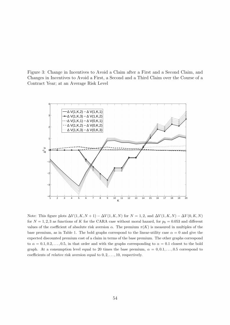
Figure 3: Change in Incentives to Avoid a Claim after a First and a Second Claim, andChanges in Incentives to Avoid a First, a Second and a Third Claim over the Course of aContract Year; at an Average Risk Level

1 2 3 4 5 6 7 8 9 10 11 12 13 14 15 16 17 18 19 20−4

−3

−2

−1

0

1

2

3

4

K

∆2 V

∆ V(1,K,2) − ∆ V(1,K,1)∆ V(1,K,3) − ∆ V(1,K,2)∆ V(1,K,1) − ∆ V(0,K,1)∆ V(1,K,2) − ∆ V(0,K,2)∆ V(1,K,3) − ∆ V(0,K,3)

Note: This figure plots ∆V (1,K,N + 1) −∆V (1,K,N) for N = 1, 2, and ∆V (1,K,N) −∆V (0,K,N)

for N = 1, 2, 3 as functions of K for the CARA case without moral hazard, for p0 = 0.053 and different

values of the coefficient of absolute risk aversion α. The premium π(K) is measured in multiples of the

base premium, as in Table 1. The bold graphs correspond to the linear-utility case α = 0 and give the

expected discounted premium cost of a claim in terms of the base premium. The other graphs correspond

to α = 0.1, 0.2, . . . , 0.5, in that order and with the graphs corresponding to α = 0.1 closest to the bold

graph. At a consumption level equal to 20 times the base premium, α = 0, 0.1, . . . , 0.5 correspond to

coefficients of relative risk aversion equal to 0, 2, . . . , 10, respectively.

54

Figure 4: Change in Incentives to Avoid a Claim after a First and a Second Claim, andChanges in Incentives to Avoid a First, a Second and a Third Claim over the Course of aContract Year; at a Zero Risk Level

1 2 3 4 5 6 7 8 9 10 11 12 13 14 15 16 17 18 19 20

−3

−2

−1

0

1

2

3

K

∆2 V

∆ V(1,K,2) − ∆ V(1,K,1)∆ V(1,K,3) − ∆ V(1,K,2)∆ V(1,K,1) − ∆ V(0,K,1)∆ V(1,K,2) − ∆ V(0,K,2)∆ V(1,K,3) − ∆ V(0,K,3)

Note: This figure plots ∆V (1,K,N + 1) −∆V (1,K,N) for N = 1, 2, and ∆V (1,K,N) −∆V (0,K,N)

for N = 1, 2, 3 as functions of K for the CARA case without moral hazard, for p0 = 0 and different

values of the coefficient of absolute risk aversion α. The premium π(K) is measured in multiples of the

base premium, as in Table 1. The bold graphs correspond to the linear-utility case α = 0 and give the

expected discounted premium cost of a claim in terms of the base premium. The other graphs correspond

to α = 0.1, 0.2, . . . , 0.5, in that order and with the graphs corresponding to α = 0.1 closest to the bold

graph. At a consumption level equal to 20 times the base premium, α = 0, 0.1, . . . , 0.5 correspond to

coefficients of relative risk aversion equal to 0, 2, . . . , 10, respectively.

55

Figure 5: Change in Incentives to Avoid a Claim after a First and a Second Claim, andChanges in Incentives to Avoid a First, a Second and a Third Claim over the Course of aContract Year; at a High Risk Level

1 2 3 4 5 6 7 8 9 10 11 12 13 14 15 16 17 18 19 20−4

−3

−2

−1

0

1

2

3

K

∆2 V

∆ V(1,K,2) − ∆ V(1,K,1)∆ V(1,K,3) − ∆ V(1,K,2)∆ V(1,K,1) − ∆ V(0,K,1)∆ V(1,K,2) − ∆ V(0,K,2)∆ V(1,K,3) − ∆ V(0,K,3)

Note: This figure plots ∆V (1,K,N + 1) −∆V (1,K,N) for N = 1, 2, and ∆V (1,K,N) −∆V (0,K,N)

for N = 1, 2, 3 as functions of K for the CARA case without moral hazard, for p0 = 0.232 and different

values of the coefficient of absolute risk aversion α. The premium π(K) is measured in multiples of the

base premium, as in Table 1. The bold graphs correspond to the linear-utility case α = 0 and give the

expected discounted premium cost of a claim in terms of the base premium. The other graphs correspond

to α = 0.1, 0.2, . . . , 0.5, in that order and with the graphs corresponding to α = 0.1 closest to the bold

graph. At a consumption level equal to 20 times the base premium, α = 0, 0.1, . . . , 0.5 correspond to

coefficients of relative risk aversion equal to 0, 2, . . . , 10, respectively.

56

Figure 6: Estimated Probability Masses ξr(K) of the Auxiliary Model (14) with ThreeMass Points

0

0.5

1BM class 1

λ1

λ2

λ3

0

0.5

1BM class 2

λ1

λ2

λ3

0

0.5

1BM class 3

λ1

λ2

λ3

0

0.5

1BM class 4

λ1

λ2

λ3

0

0.5

1BM class 5

λ1

λ2

λ3

0

0.5

1BM class 6

λ1

λ2

λ3

0

0.5

1BM class 7

λ1

λ2

λ3

0

0.5

1BM class 8

λ1

λ2

λ3

0

0.5

1BM class 9

λ1

λ2

λ3

0

0.5

1BM class 10

λ1

λ2

λ3

0

0.5

1BM class 11

λ1

λ2

λ3

0

0.5

1BM class 12

λ1

λ2

λ3

0

0.5

1BM class 13

λ1

λ2

λ3

0

0.5

1BM class 14

λ1

λ2

λ3

0

0.5

1BM class 15

λ1

λ2

λ3

0

0.5

1BM class 16

λ1

λ2

λ3

0

0.5

1BM class 17

λ1

λ2

λ3

0

0.5

1BM class 18

λ1

λ2

λ3

0

0.5

1BM class 19

λ1

λ2

λ3

0

0.5

1BM class 20

λ1

λ2

λ3

57

Figure 7: Comparison of H1 with the Uniform Distribution for Low and High Bonus-MalusClasses

0 0.1 0.2 0.3 0.4 0.5 0.6 0.7 0.8 0.9 10

0.1

0.2

0.3

0.4

0.5

0.6

0.7

0.8

0.9

1

t

H1

Uniform CDF Empirical H

1 for low BM 1 − 10

Empirical H1 for high BM 11 − 20

58

Figure 8: Comparison of H1 with the Uniform Distribution and of H21 with H2 for Low

and High Bonus-Malus Classes, with H1 and H2 Estimated on the Same Classes

0 0.1 0.2 0.3 0.4 0.5 0.6 0.7 0.8 0.9 10

0.1

0.2

0.3

0.4

0.5

0.6

0.7

0.8

0.9

1

t

Low BM classes 1 − 10

Uniform CDF Empirical H

1

Empirical H12

Empirical H2

0 0.1 0.2 0.3 0.4 0.5 0.6 0.7 0.8 0.9 10

0.1

0.2

0.3

0.4

0.5

0.6

0.7

0.8

0.9

1

t

High BM classes 11 − 20

Uniform CDF Empirical H

1

Empirical H12

Empirical H2

59

Figure 9: Share of Withdrawn Claims per Bonus-Malus Class

1 2 3 4 5 6 7 8 9 10 11 12 13 14 15 16 17 18 19 200%

1%

2%

3%

4%

5%

6%

7%

8%

BM class

Sha

re

Withdrawals

Note: This graph only includes withdrawals that are directly observed. See Appendix C.

60

Table 1: Bonus-Malus Scheme

Present Premium Future BM class (B(K,N)) after a contract year withBM class paid no claim 1 claim 2 claims 3 or more claims

(K) (q = A(K)) (N = 0) (N = 1) (N = 2) (N ≥ 3)

20 25% 20 14 8 119 25% 20 13 7 118 25% 19 12 7 117 25% 18 11 6 116 25% 17 10 6 115 25% 16 9 5 114 25% 15 8 4 113 30% 14 7 3 112 35% 13 7 3 111 37.5% 12 6 2 110 40% 11 6 2 19 45% 10 5 1 18 50% 9 4 1 17 55% 8 3 1 16 60% 7 2 1 15 70% 6 1 1 14 80% 5 1 1 13 90% 4 1 1 12 100% 3 1 1 11 120% 2 1 1 1

Note: The notation in parentheses is taken from Section 3’s model.

61

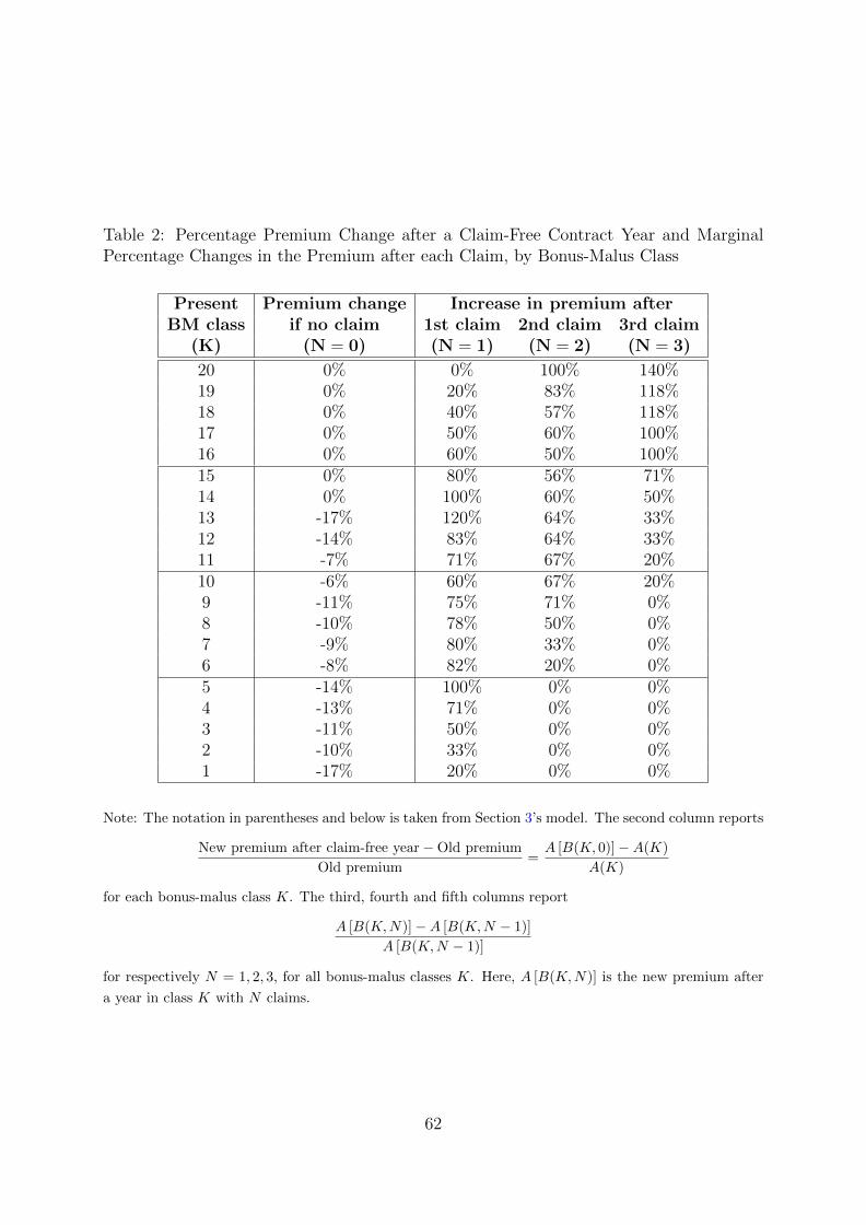
Table 2: Percentage Premium Change after a Claim-Free Contract Year and MarginalPercentage Changes in the Premium after each Claim, by Bonus-Malus Class

Present Premium change Increase in premium afterBM class if no claim 1st claim 2nd claim 3rd claim

(K) (N = 0) (N = 1) (N = 2) (N = 3)

20 0% 0% 100% 140%19 0% 20% 83% 118%18 0% 40% 57% 118%17 0% 50% 60% 100%16 0% 60% 50% 100%15 0% 80% 56% 71%14 0% 100% 60% 50%13 -17% 120% 64% 33%12 -14% 83% 64% 33%11 -7% 71% 67% 20%10 -6% 60% 67% 20%9 -11% 75% 71% 0%8 -10% 78% 50% 0%7 -9% 80% 33% 0%6 -8% 82% 20% 0%5 -14% 100% 0% 0%4 -13% 71% 0% 0%3 -11% 50% 0% 0%2 -10% 33% 0% 0%1 -17% 20% 0% 0%

Note: The notation in parentheses and below is taken from Section 3’s model. The second column reports

New premium after claim-free year−Old premium

Old premium=A [B(K, 0)]−A(K)

A(K)

for each bonus-malus class K. The third, fourth and fifth columns report

A [B(K,N)]−A [B(K,N − 1)]

A [B(K,N − 1)]

for respectively N = 1, 2, 3, for all bonus-malus classes K. Here, A [B(K,N)] is the new premium after

a year in class K with N claims.

62

Table 3: Contract Exposure Durations in the Sample

Number of years Number of contracts observedY exactly Y years between Y − 1 and Y years Total1 8,097 11,775 19,8722 4,709 9,616 14,3253 6,262 7,387 13,6494 68,820 6,503 75,323

Total 87,888 35,281 123,169

63

Table 4: Number of Contracts Observed for At Least One Full Contract Year, by Bonus-Malus Class and Number of Claims in the First Contract Year

BM Number of contracts withclass no claim 1 claim 2 claims 3 claims 4 claims Total

1 562 118 24 4 1 7092 749 94 11 1 8553 962 81 10 1,0534 1,311 100 9 1,4205 1,876 112 13 1 2,0026 2,514 160 14 2 2,6907 3,363 207 16 3,5868 4,232 273 16 4,5219 4,889 249 15 2 5,15510 6,490 293 11 1 6,79511 6,063 279 12 2 6,35612 6,004 285 16 6,30513 5,879 266 11 6,15614 6,669 311 13 6,99315 6,165 301 6 6,47216 6,377 297 13 1 6,68817 5,671 249 7 5,92718 4,367 204 10 4,58119 3,855 214 5 4,07420 27,652 1,373 29 2 29,056

Total 105,650 5,466 261 15 2 111,394

Note: Nil and withdrawn claims were excluded from the sample.

64

Table 5: Maximum-Likelihood Estimation of the Auxiliary Model (14) with Three, Four,and Five Support Points

Three Support Points

Parameter Estimate Std. Errorβ 0.4229 0.0428λ1 0.0427 0.0050λ2 0.1770 0.0254λ3 0.3514 0.0234

Tests of β = 0

• LM test: 26.14, p-value = 0.00

• LR test: 89.74, p-value = 0.00

• Wald test: 97.54, p-value = 0.00

Four Support Points

Parameter Estimate Std. Errorβ 0.3810 0.0337λ1 0.0000 0.0000λ2 0.0552 0.0074λ3 0.2211 0.0125λ4 0.8715 0.1260

Tests of β = 0

• LM test: 72.73, p-value = 0.00

• LR test: 94.96, p-value = 0.00

• Wald test: 127.90, p-value = 0.00

Five Support Points

Parameter Estimate Std. Errorβ 0.4017 0.0390λ1 0.0135 0.0118λ2 0.0531 0.0117λ3 0.1889 0.0164λ4 0.2629 0.0171λ5 0.8896 0.1219

Tests of β = 0

• LM test: 76.56, p-value = 0.00

• LR test: 106.39, p-value = 0.00

• Wald test: 106.09, p-value = 0.00

Note: The left side of each panel presents maximum-likelihood estimates of the relevant parameters in

the unrestricted auxiliary model (14). The right side of each panel presents Lagrange multiplier (LM),

likelihood-ratio (LR) and Wald tests for moral hazard.

65

Table 6: Nonparametric Tests Based on Comparison of H1 and H2 for Different Bonus-Malus Classes

Kruskal - Wallis test p-valueH1(K) equal for all K 0.592H2(K) equal for all K 0.271

Wilcoxon test p-valueH1(low K) ∼ H1(high K) 0.629H2(low K) ∼ H2(high K) 0.006

Kolmogorov - Smirnov test p-valueH1(low K) ∼ H1(high K) 0.676H2(low K) ∼ H2(high K) 0.004

Note: This table is computed using a subsample of first fully-observed contract years from Table 4’s

sample. The values in bold imply rejection of the null of no moral hazard at a 5% level. Low classes are

BM classes 1 – 10 and high classes are BM classes 11 – 20.

66

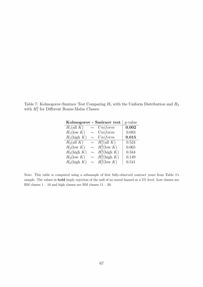
Table 7: Kolmogorov-Smirnov Test Comparing H1 with the Uniform Distribution and H2

with H21 for Different Bonus-Malus Classes

Kolmogorov - Smirnov test p-valueH1(all K) ∼ Uniform 0.002H1(low K) ∼ Uniform 0.083H1(high K) ∼ Uniform 0.015H2(all K) ∼ H2

1 (all K) 0.524H2(low K) ∼ H2

1 (low K) 0.065H2(high K) ∼ H2

1 (high K) 0.344H2(low K) ∼ H2

1 (high K) 0.149H2(high K) ∼ H2

1 (low K) 0.541

Note: This table is computed using a subsample of first fully-observed contract years from Table 4’s

sample. The values in bold imply rejection of the null of no moral hazard at a 5% level. Low classes are

BM classes 1 – 10 and high classes are BM classes 11 – 20.

67

Table 8: Tests Based on Comparison of First and Second Claim Durations, for DifferentBonus-Malus Classes

BM Test statistics (std. error)

classes πn ln βn π∗n(all) π∗n(current)1 62.5% (10.2%) 0.392 (0.370) 54.2% (10.2%) 54.2% (10.9%)

1 – 2 65.7% (8.5%) 0.570 (0.307) 60.0% (8.5%) 60.0% (8.9%)1 – 3 62.2% (7.5%) 0.384 (0.270) 57.8% (7.5%) 57.8% (7.8%)1 – 4 55.6% (6.8%) 0.211 (0.247) 51.9% (6.8%) 53.7% (7.1%)1 – 5 55.2% (6.1%) 0.180 (0.222) 52.2% (6.1%) 55.2% (6.4%)1 – 6 54.3% (5.6%) 0.046 (0.202) 50.6% (5.6%) 54.3% (5.8%)1 – 7 53.6% (5.1%) 0.086 (0.184) 50.5% (5.1%) 53.6% (5.3%)1 – 8 53.1% (4.7%) 0.085 (0.171) 50.4% (4.7%) 53.1% (4.9%)1 – 9 52.3% (4.4%) 0.083 (0.160) 49.2% (4.5%) 50.8% (4.6%)1 – 10 53.2% (4.2%) 0.106 (0.154) 50.4% (4.3%) 51.1% (4.4%)

All 52.9% (3.1%) 0.107 (0.112) 50.6% (3.1%) 50.6% (3.1%)11 – 20 52.5% (4.5%) 0.109 (0.164) 50.8% (4.6%) 50.8% (4.6%)12 – 20 51.8% (4.8%) 0.035 (0.173) 50.0% (4.8%) 50.0% (4.8%)13 – 20 51.1% (5.2%) 0.070 (0.187) 50.0% (5.2%) 50.0% (5.2%)14 – 20 53.0% (5.5%) 0.132 (0.199) 51.8% (5.5%) 51.8% (5.5%)15 – 20 51.4% (6.0%) 0.101 (0.217) 50.0% (6.0%) 50.0% (6.0%)16 – 20 48.4% (6.3%) -0.040 (0.227) 46.9% (6.3%) 46.9% (6.3%)17 – 20 45.1% (7.0%) -0.188 (0.254) 43.1% (7.0%) 43.1% (7.1%)18 – 20 47.7% (7.5%) -0.105 (0.273) 45.5% (7.6%) 47.7% (7.6%)19 – 20 44.1% (8.6%) -0.057 (0.311) 41.2% (8.6%) 44.1% (8.6%)

20 41.4% (9.3%) -0.112 (0.337) 41.4% (9.3%) 44.8% (9.3%)

Note: This table is computed using a subsample of first fully-observed contract years from Table 4’s

sample. The values in bold imply rejection of the null of no moral hazard at a 5% level (two-sided test).

In the computation of π∗n, we first used all bonus-malus classes to estimate H1, and then only the tested

(current) bonus-malus classes listed in the first column.

68

Table 9: Tests Based on Comparison of First and Second Claim Durations that Pool Lowand High Bonus-Malus Classes

BM classes Test statistics (std. error)

low high πn ln βn π∗n(all) π∗n(current)1 20 60.4% (6.9%) 0.239 (0.249) 56.6% (6.9%) 56.6% (6.9%)

1 – 2 20 62.5% (6.3%) 0.363 (0.227) 59.4% (6.3%) 59.4% (6.3%)1 – 2 19 – 20 60.9% (6.0%) 0.317 (0.218) 59.4% (6.0%) 59.4% (6.1%)1 – 2 18 – 20 58.2% (5.6%) 0.311 (0.204) 57.0% (5.7%) 58.2% (5.7%)1 – 2 17 – 20 59.3% (5.4%) 0.343 (0.196) 58.1% (5.4%) 58.1% (5.5%)1 – 3 19 – 20 59.5% (5.6%) 0.243 (0.204) 58.2% (5.7%) 58.2% (5.7%)1 – 3 18 – 20 57.3% (5.3%) 0.246 (0.192) 56.2% (5.3%) 57.3% (5.4%)1 – 4 17 – 20 55.2% (4.9%) 0.200 (0.177) 54.3% (4.9%) 54.3% (4.9%)1 – 5 16 – 20 53.4% (4.4%) 0.112 (0.158) 52.7% (4.4%) 52.7% (4.4%)1 – 6 15 – 20 51.7% (4.1%) -0.022 (0.148) 50.3% (4.1%) 50.3% (4.1%)1 – 7 14 – 20 50.6% (3.7%) -0.014 (0.135) 49.4% (3.8%) 49.4% (3.8%)1 – 8 13 – 20 51.2% (3.5%) 0.015 (0.126) 50.2% (3.5%) 50.2% (3.5%)1 – 9 12 – 20 50.4% (3.2%) 0.028 (0.118) 49.6% (3.3%) 49.6% (3.3%)1 – 10 11 – 20 50.6% (3.1%) 0.006 (0.112) 49.8% (3.1%) 49.8% (3.1%)

Note: This table is computed using a subsample of first fully-observed contract years from Table 4’s

sample. The values in bold imply rejection of the null of no moral hazard at a 5% level (one-sided test).

In the computation of π∗n, we first used all bonus-malus classes to estimate H1, and then only the tested

(current) bonus-malus classes listed in the first column.

69

Table 10: Comparison of First and Second Claim Sizes for Various Bonus-Malus Classes

BM # Wilcoxon test Sign test L1 ∼ L2 againstclasses obs. p-value L1 � L2 L1 ≺ L2 L1 6∼ L2

1 29 0.336 0.068 0.969 0.1361 – 2 41 0.791 0.378 0.734 0.7551 – 3 51 0.633 0.500 0.610 1.0001 – 4 60 0.802 0.449 0.651 0.8971 – 5 74 0.942 0.546 0.546 1.0001 – 6 90 0.755 0.701 0.376 0.7521 – 7 106 0.458 0.809 0.248 0.4971 – 8 122 0.219 0.913 0.120 0.2391 – 9 139 0.173 0.913 0.117 0.2351 – 10 151 0.240 0.873 0.164 0.329

All 278 0.028 0.993 0.010 0.01911 – 20 127 0.061 0.994 0.010 0.02112 – 20 113 0.043 0.996 0.007 0.01413 – 20 97 0.035 0.993 0.012 0.02514 – 20 86 0.029 0.994 0.011 0.02315 – 20 73 0.055 0.995 0.009 0.01916 – 20 67 0.038 0.998 0.003 0.00717 – 20 53 0.090 0.986 0.027 0.05318 – 20 46 0.127 0.973 0.052 0.10419 – 20 36 0.388 0.879 0.203 0.405

20 31 0.493 0.763 0.360 0.720

Note: This table is computed using a subsample of contracts with at least two claims in the first fully-

observed contract year from the Table 4’s sample. The values in bold imply rejection of the null of no

moral hazard at a 5% level.

70