Stock assessment of bigeye tuna in the western and central Pacific Ocean

John Hampton

Oceanic Fisheries Programme

Secretariat of the Pacific Community

Noumea, New Caledonia.

SCTB15 Working Paper

BET−1

1

1 IntroductionThis paper describes the application of a length-based, age-structured, spatially-disaggregated

model known as MULTIFAN-CL (Fournier et al. 1998; Hampton and Fournier 2001) to bigeye tunain the western and central Pacific Ocean (WCPO). A separate analysis treating the entire PacificOcean is also available.

2 Background

2.1 BiologyBigeye tuna are distributed throughout the tropical and sub-tropical waters of the Pacific

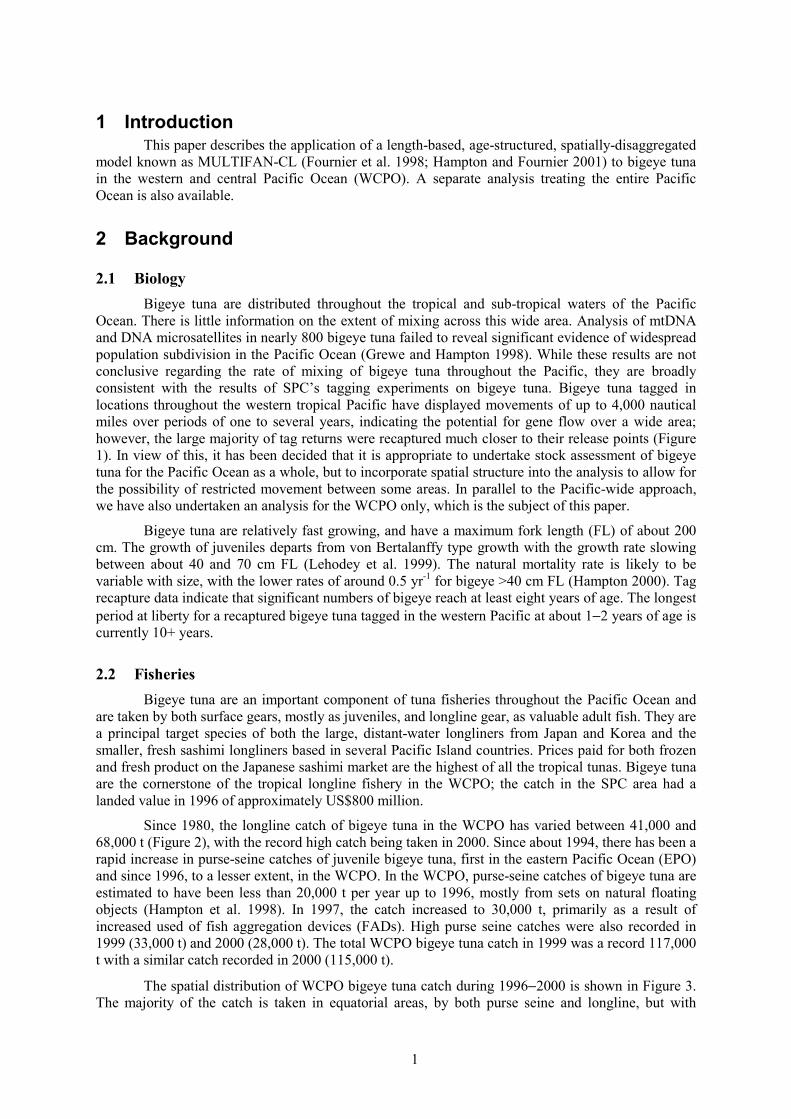
Ocean. There is little information on the extent of mixing across this wide area. Analysis of mtDNAand DNA microsatellites in nearly 800 bigeye tuna failed to reveal significant evidence of widespreadpopulation subdivision in the Pacific Ocean (Grewe and Hampton 1998). While these results are notconclusive regarding the rate of mixing of bigeye tuna throughout the Pacific, they are broadlyconsistent with the results of SPC’s tagging experiments on bigeye tuna. Bigeye tuna tagged inlocations throughout the western tropical Pacific have displayed movements of up to 4,000 nauticalmiles over periods of one to several years, indicating the potential for gene flow over a wide area;however, the large majority of tag returns were recaptured much closer to their release points (Figure1). In view of this, it has been decided that it is appropriate to undertake stock assessment of bigeyetuna for the Pacific Ocean as a whole, but to incorporate spatial structure into the analysis to allow forthe possibility of restricted movement between some areas. In parallel to the Pacific-wide approach,we have also undertaken an analysis for the WCPO only, which is the subject of this paper.

Bigeye tuna are relatively fast growing, and have a maximum fork length (FL) of about 200cm. The growth of juveniles departs from von Bertalanffy type growth with the growth rate slowingbetween about 40 and 70 cm FL (Lehodey et al. 1999). The natural mortality rate is likely to bevariable with size, with the lower rates of around 0.5 yr-1 for bigeye >40 cm FL (Hampton 2000). Tagrecapture data indicate that significant numbers of bigeye reach at least eight years of age. The longestperiod at liberty for a recaptured bigeye tuna tagged in the western Pacific at about 1−2 years of age iscurrently 10+ years.

2.2 FisheriesBigeye tuna are an important component of tuna fisheries throughout the Pacific Ocean and

are taken by both surface gears, mostly as juveniles, and longline gear, as valuable adult fish. They area principal target species of both the large, distant-water longliners from Japan and Korea and thesmaller, fresh sashimi longliners based in several Pacific Island countries. Prices paid for both frozenand fresh product on the Japanese sashimi market are the highest of all the tropical tunas. Bigeye tunaare the cornerstone of the tropical longline fishery in the WCPO; the catch in the SPC area had alanded value in 1996 of approximately US$800 million.

Since 1980, the longline catch of bigeye tuna in the WCPO has varied between 41,000 and68,000 t (Figure 2), with the record high catch being taken in 2000. Since about 1994, there has been arapid increase in purse-seine catches of juvenile bigeye tuna, first in the eastern Pacific Ocean (EPO)and since 1996, to a lesser extent, in the WCPO. In the WCPO, purse-seine catches of bigeye tuna areestimated to have been less than 20,000 t per year up to 1996, mostly from sets on natural floatingobjects (Hampton et al. 1998). In 1997, the catch increased to 30,000 t, primarily as a result ofincreased used of fish aggregation devices (FADs). High purse seine catches were also recorded in1999 (33,000 t) and 2000 (28,000 t). The total WCPO bigeye tuna catch in 1999 was a record 117,000t with a similar catch recorded in 2000 (115,000 t).

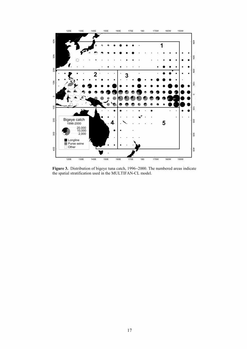
The spatial distribution of WCPO bigeye tuna catch during 1996−2000 is shown in Figure 3.The majority of the catch is taken in equatorial areas, by both purse seine and longline, but with

2

significant longline catch in some sub-tropical areas (east of Japan, northeast of Hawaii and the eastcoast of Australia). High catches are also presumed to be taken in the domestic artisanal fisheries ofPhilippines and Indonesia. These catches, along with small catches by pole-and-line vessels operatingin various parts of the WCPO, have approached 20,000 t in recent years. The statistical basis for thecatch estimates in Philippines and Indonesia is weak; however, we have included the best availableestimates in this analysis in the interests of providing the best possible coverage of the WCPO.

3 Data compilationThe data used in the bigeye tuna assessment consist of catch, effort, length-frequency and

weight-frequency data for the fisheries defined in the analysis, and tag release-recapture data. Thedetails of these data and their stratification are described below.

3.1 Spatial stratificationThe geographic area considered in the assessment is the WCPO, defined by the coordinates

40°N−35°S, 120°E−150°W. Within this overall area, a five-region spatial stratification was adoptedfor the assessment (Figure 3).

3.2 Temporal stratificationThe time period covered by the assessment is 1962−2001. Within this period, data were

compiled into quarters (Jan−Mar, Apr−Jun, Jul−Sep, Oct−Dec).

3.3 Definition of fisheriesMULTIFAN-CL requires the definition of “fisheries” that consist of relatively homogeneous

fishing units. Ideally, the fisheries so defined will have selectivity and catchability characteristics thatdo not vary greatly over time (although in the case of catchability, some allowance can be made fortime-series variation). For most pelagic fisheries assessments, fisheries defined according to gear type,fishing method and region will usually suffice. Fifteen fisheries have been defined for this analysis(Table 1).

3.4 Catch and effort dataCatch and effort data were compiled according to the fisheries defined above. Catches by the

longline fisheries were expressed in numbers of fish, and catches for all other fisheries expressed inweight. Purse seine catches of bigeye are not reliably recorded on logsheets for most fleets, and mustbe estimated from sampling data. The methods used to derive such estimates for the purse seinefishery are described in OFP (2002).

Effort data for the Philippines and Indonesian fisheries were unavailable and defined asmissing. Effort data units for purse seine fisheries are defined as days fishing and/or searching,allocated to set types based on the proportion of total sets attributed to a specified set type (log, FADor school sets) in logbook data. For the longline fisheries, we used estimates of effective effortderived in a separate study (Bigelow et al. 2002, updated to include 2000 data). Essentially, effectiveeffort is an estimate of the numbers of longline hooks fishing in the region of the water column that isassumed to define bigeye tuna habitat. In this study, bigeye tuna habitat was defined in terms of watertemperature preferences indicated from a sonic tracking study (Dagorn et al. 2000) carried out in aregion of high longline bigeye catches (central tropical Pacific), and oxygen requirements as indicatedby laboratory and other studies (Brill 1994). The estimates take into account the time and spatialvariability in the depth of bigeye tuna habitat (using oceanographic databases) and variation in thefishing depth of longliners as indicated by distributions of the numbers of hooks between floats. Theeffective effort estimates were derived at 5°-month resolution for the Japanese distant-water longlinefleet and raised to represent the total longline catch by 5°-month before aggregating into the four-

3

region-quarterly stratification used in the model. Longline effort data were not available for 2001 −we assumed the same levels of effective effort as the corresponding quarters of 2000 and declared thecatches for 2001 to be missing.

Within the model, effort for each fishery was normalized to an average of 1.0 to assistnumerical stability. In the case of the longline fisheries, the normalization occurred over the five “allnationalities” fisheries rather than individually. Also, effort for these fisheries was divided by therelative size of the respective region. The application of these procedures allowed longline CPUE toindex exploitable abundance in each region (rather than density), which in turn allowed simplifyingassumptions to be made regarding the spatial and temporal constancy of catchability for the longlinefisheries.

3.5 Length-frequency dataAvailable length-frequency data for each of the defined fisheries were compiled into 100 2-

cm size classes (10−12 cm to 208−210 cm). Each length-frequency observation consisted of the actualnumber of bigeye tuna measured. The data were collected from a variety of sampling programmes,which can be summarized as follows:

Philippines: Size composition data for the Philippines domestic fisheries derived from a samplingprogramme conducted in the Philippines in 1993−94 have recently been augmented with data from the1980s and for 1995.

Indonesia: Limited size data were obtained for the Indonesian domestic fisheries from the formerIPTP database. Under the assumption that most of the catch is by pole-and-line gear, catches by theSPC tagging vessels operating in Indonesia in 1980 and 1991−93 have also been used to represent thesize composition of domestic fishery catches.

Purse seine: Length-frequency samples from purse seiners have been collected from a variety of portsampling programmes since the mid-1980s. Most of the early data is sourced from the U.S. NationalMarine Fisheries Service (NMFS) port sampling programme for U.S. purse seiners in Pago Pago,American Samoa and an observer programme conducted for the same fleet. Since the early 1990s,port sampling and observer programmes on other purse seine fleets have provided additional data.Only data that could be classified by set type were included in the final data set.

Longline: The majority of the historical data were collected by port sampling programmes forJapanese longliners unloading in Japan and from sampling aboard Japanese research and trainingvessels. It is assumed that these data are representative of the sizes of longline-caught bigeyegenerally in the WCPO. In recent years, data have also been collected by OFP and national portsampling and observer programmes in the WCPO.

3.6 Weight-frequency dataIndividual weight data are available for several longline fisheries. In some cases (e.g. the

Australian longline fishery), the weight data represent a large proportion of the total catch. In additionto the Australian fishery, weight data are also available from vessels unloading in Guam and fromvarious unloading ports around the region where tuna are exported. Data were compiled by 1 kgweight intervals over a range of 1−120 kg. As the weights were generally gilled-and-gutted weights,the frequency intervals were adjusted by a gilled-and-gutted to whole weight conversion factor forbigeye tuna (1.1018).

3.7 Tagging dataA large amount of tagging data was available for incorporation into the MULTIFAN-CL

analysis. The data used consisted of bigeye tuna tag releases and returns from the OFP’s RegionalTuna Tagging Project conducted during 1989−1992. Trained scientists and technicians released tagsusing standard tuna tagging equipment and techniques. The tag release effort was spread throughout

4

the tropical western Pacific, between approximately 120°E and 170°W (see Kaltongga 1998 forfurther details).

For incorporation into the MULTIFAN-CL analysis, tag releases are stratified by releaseregion (all bigeye tuna releases occurred in regions 2, 3, 4 and 5), time period of release (quarter) andthe same length classes used to stratify the length-frequency data. A total of 7,903 releases wereclassified into 20 tag release groups in this way. Of the 1,003 tag returns in total, 870 could beassigned to the fisheries included in the model. Tag returns that could not be so assigned wereincluded in the non-reported category and appropriate adjustments made to the tag-reporting rateparameters. The returns from each size class of each tag release group were then classified byrecapture fishery and recapture time period (quarter). Because tag returns by purse seiners were oftennot accompanied by information concerning the set type, tag-return data were aggregated across settypes for the purse seine fisheries in each region. The population dynamics model was in turnconfigured to predict equivalent estimated tag recaptures by these grouped fisheries.

4 Structural assumptions of the modelAs with any model, various structural assumptions have been made in the bigeye tuna model.

Such assumptions are always a trade-off to some extent between the need, on the one hand, to keepthe parameterization as simple as possible, and on the other, to allow sufficient flexibility so thatimportant characteristics of the fisheries and population are captured in the model. The mathematicalspecification of structural assumptions is described in general terms in Hampton and Fournier (2001).The main structural assumptions used in the bigeye tuna model are discussed below and aresummarized in Table 2.

4.1 Observation models for the dataThere are four data components that contribute to the log-likelihood function − the total catch

data, the length-frequency data, the weight-frequency data and the tagging data. The observed totalcatch data are assumed to be unbiased and relatively precise, with the SD of residuals on the log scalebeing 0.07.

The probability distributions for the length-frequency proportions are assumed to beapproximated by robust normal distributions, with the variance determined by the effective samplesize and the observed length-frequency proportion. Effective sample size is assumed to be 0.1 timesthe actual sample size for non-longline fisheries and 0.2 times the actual sample size for longlinefisheries, with a maximum effective sample size for all fisheries of 1000. Reduction of the effectivesample size recognises that length-frequency samples are not truly random and would have highervariance as a result. The differential treatment of longline and purse seine fisheries occurs becausesampling coverage of purse seine catches is generally lower than longline, and the purse seinesamples tend to be clumped by wells.

A similar likelihood function was used for the weight-frequency data. The only exception wasthat the effective sample size for the Australian longline fishery was assumed to be equal to the actualsample size because the sample coverage represented a high proportion of the catch thus increasingthe likelihood that the samples were random.

A log-likelihood component for the tag data was computed using a negative binomialdistribution in which fishery-specific variance parameters were estimated from the data. The negativebinomial is preferred over the more commonly used Poisson distribution because tagging data oftenexhibit more variability than can be attributed by the Poisson. We have employed a parameterizationof the variance parameters such that as they approach infinity, the negative binomial approaches thePoisson. Therefore, if the tag return data show high variability (for example, due to contagion or non-independence of tags), then the negative binomial is able to recognise this. This would then provide amore realistic weighting of the tag return data in the overall log-likelihood and allow the variability toimpact the confidence intervals of estimated parameters. A complete derivation and description of the

5

negative binomial likelihood function for tagging data is provided in Hampton and Fournier (2001)(Appendix C).

4.2 Tag reportingWhile the model has the capacity to estimate tag-reporting rates, we provided Bayesian priors

for fishery-specific reporting rates. Relatively informative priors were provided for reporting rates forthe Philippines and Indonesian domestic fisheries and the purse seine fisheries, as independentestimates of reporting rates for these fisheries were available from tag seeding experiments and otherinformation (Hampton 1997). For the longline fisheries L1−L5, we have no auxiliary information withwhich to estimate reporting rates, so a relatively uninformative prior was used and a commonreporting rate estimated. All reporting rates were assumed to be stable over time. The proportions oftag returns rejected from the analysis because of insufficient data were incorporated into the reportingrate priors.

4.3 Tag mixingWe assume that tagged bigeye gradually mix with the untagged population at the region level

and that this mixing process is complete by the second quarter after release.

4.4 Recruitment“Recruitment” in terms of the MULTIFAN-CL model is the appearance of age-class 1 fish in

the population. We assumed that there are four recruitments per year, which occur at the start of eachquarter. This is an approximation to continuous recruitment.

The distribution of recruitment among the five model regions was estimated and allowed tovary over time in an unconstrained fashion. The time-series variation in spatially-aggregatedrecruitment was somewhat constrained by a lognormal prior. The variance of the prior was set suchthat recruitments of about three times and one third of the average recruitment would occur aboutonce every 25 years on average.

Spatially-aggregated recruitment was assumed to have a weak relationship with the parentalbiomass via a Beverton and Holt stock-recruitment relationship (SRR). The SRR was incorporatedmainly so that a yield analysis could be undertaken for stock assessment purposes. We therefore optedto apply a relatively weak penalty for deviation from the SRR so that it would have only a slight effecton the recruitment and other model estimates (see Hampton and Fournier 2001, Appendix D).

Typically, fisheries data are very uninformative about SRR parameters and it is generallynecessary to constrain the parameterisation in order to have stable model behaviour. We haveincorporated a beta-distributed prior on the “steepness” (S) of the SRR, with S defined as the ratio ofthe equilibrium recruitment produced by 20% of the equilibrium unexploited spawning biomass tothat produced by the equilibrium unexploited spawning biomass (Francis 1992; Maunder and Watters2001). The prior was specified by mode = 0.9 and SD = 0.04 (a = 46, b = 6). In other words, our priorbelief is that the reduction in equilibrium recruitment when the equilibrium spawning biomass isreduced to 20% of its unexploited level would be fairly small (a decline of 10%).

4.5 Age and growthThe standard assumptions made concerning age and growth in the MULTIFAN-CL model are

(i) the lengths-at-age are assumed to be normally distributed for each age-class; (ii) the mean lengths-at-age are assumed to follow a von Bertalanffy growth curve; (iii) the standard deviations of lengthfor each age-class are assumed to be a linear function of the mean length-at-age; and (iv) theprobability distributions of weights-at-age are a deterministic function of the lengths-at-age and aspecified weight-length relationship (see Table 2).

6

For any specific model, it is necessary to assume the number of significant age-classes in theexploited population, with the last age-class being defined as a “plus group”, i.e. all fish of thedesignated age and older. This is a common assumption for any age-structured model. For the resultspresented here, 28 quarterly age-classes have been assumed.

Previous analyses assuming a standard von Bertalanffy growth pattern indicated that therewas substantial departure from the model, particularly for sizes up to about 80 cm. Similarobservations have been made on bigeye tuna growth patterns determined from daily otolithincrements and tagging data (Lehodey et al. 1999). We therefore modelled growth by allowing themean lengths of the first eight quarterly age-classes to be independent parameters, with the last twentymean lengths following a von Bertalanffy growth curve.

4.6 SelectivitySelectivity is fishery-specific and was assumed to be time-invariant. Selectivity coefficients

have a range of 0−1, and for the longline fisheries (which catch mainly adult bigeye) were assumed toincrease with age and to remain at the maximum once attained. Selectivities for longline fisheriesL1−L5 were constrained to be equal.

The selectivity coefficients are expressed as age-specific parameters, but were smoothedaccording to the degree of length overlap between adjacent age-classes. This is appropriate whereselectivity is thought to be a fundamentally length-based process (Fournier et al. 1998). Thecoefficients for the last four age-classes, for which the mean lengths are very similar, are constrainedto be equal for all fisheries.

4.7 CatchabilityCatchability was allowed to vary slowly over time (akin to a random walk) for all non-

longline fisheries and the Australian longline fishery using a structural time-series approach, andseasonally for all fisheries apart from the Philippines and Indonesian fisheries (in which the data werebased on annual estimates). Random walk steps were taken every two years, and the deviations wereconstrained by prior distributions of mean zero and variance specified for the different fisheriesaccording to our prior belief regarding the extent to which catchability may have changed. For thePhilippines and Indonesian fisheries, no effort estimates were available. We made the priorassumption that effort for these fisheries was proportional to catch, but set the variance of the priors tobe high (equivalent to a CV of about 0.7 on the log scale), thus allowing catchability changes tocompensate for failure of this assumption. For the purse seine fisheries, the catchability deviationpriors were assigned a variance equivalent to a CV of 0.10 on the log scale. We assumed thatcatchability for the non-Australian longline fisheries varied seasonally, but that their average annualvalue was both constant over time and among the different regions (fisheries). This assumptionseemed reasonable given that the estimation of “effective” fishing effort was designed to removespatial and temporal variability in CPUE due to targeting changes and variation in the depth ofoptimal bigeye tuna habitat. In essence, we allowed longline CPUE constructed using effective effortto index the exploitable abundance both among areas and over time.

4.8 Effort variabilityEffort deviations, constrained by prior distributions of zero mean, were used to model the

random variation in the effort – fishing mortality relationship. For the Philippines and Indonesianfisheries, for which reliable effort data were unavailable, we set the prior variance at a high level(equivalent to a CV of about 0.7 on the log scale), to allow the effort deviations to account forfluctuations in the catch caused by variation in real effort. For the purse seine fisheries and theAustralian longline fishery, the variance was set at a moderate level (CV of about 0.2). For the L1−L5longline fisheries, the variance was set at a low level (CV of about 0.1) to reflect our assumption thatlongline CPUE (using the effective effort estimates) provides a relatively good index of abundance.

7

4.9 MovementMovement was assumed to be time invariant and to occur instantaneously at the beginning of

each quarter. For age-independent movement, there would be two non-zero transfer coefficients foreach region boundary, i.e. 12 transfer coefficients. We allowed each of these coefficients to be age-dependent in a simple linear fashion, enabling the rate of movement across each region boundary toincrease or decrease linearly with age.

4.10 Natural mortalityNatural mortality was assumed to be age-specific, but invariant over time and region.

Penalties on the first difference, second difference and deviations from the mean were applied torestrict the age-specific variability to a certain extent.

4.11 Initial populationThe population age structure in the initial time period in each region is determined as a

function of the average total mortality during the first 20 quarters and the average recruitment inquarters 2−20 in each region. This assumption avoids having to treat the initial age structure, which isgenerally poorly determined, as independent parameters in the model.

5 Results of the base-case analysis

5.1 Fit of the model to the dataThe fit to the total catch data by fishery is very good (Figure 5), which reflects our assumption

that observation errors in the total catch estimates are relatively small.

The fit to the length data is displayed in Figure 6 for length samples aggregated over time foreach fishery. This provides a convenient means of assessing the overall fit of the model to the lengthdata for each fishery. On the whole, the model appears to have captured the main features of the data.

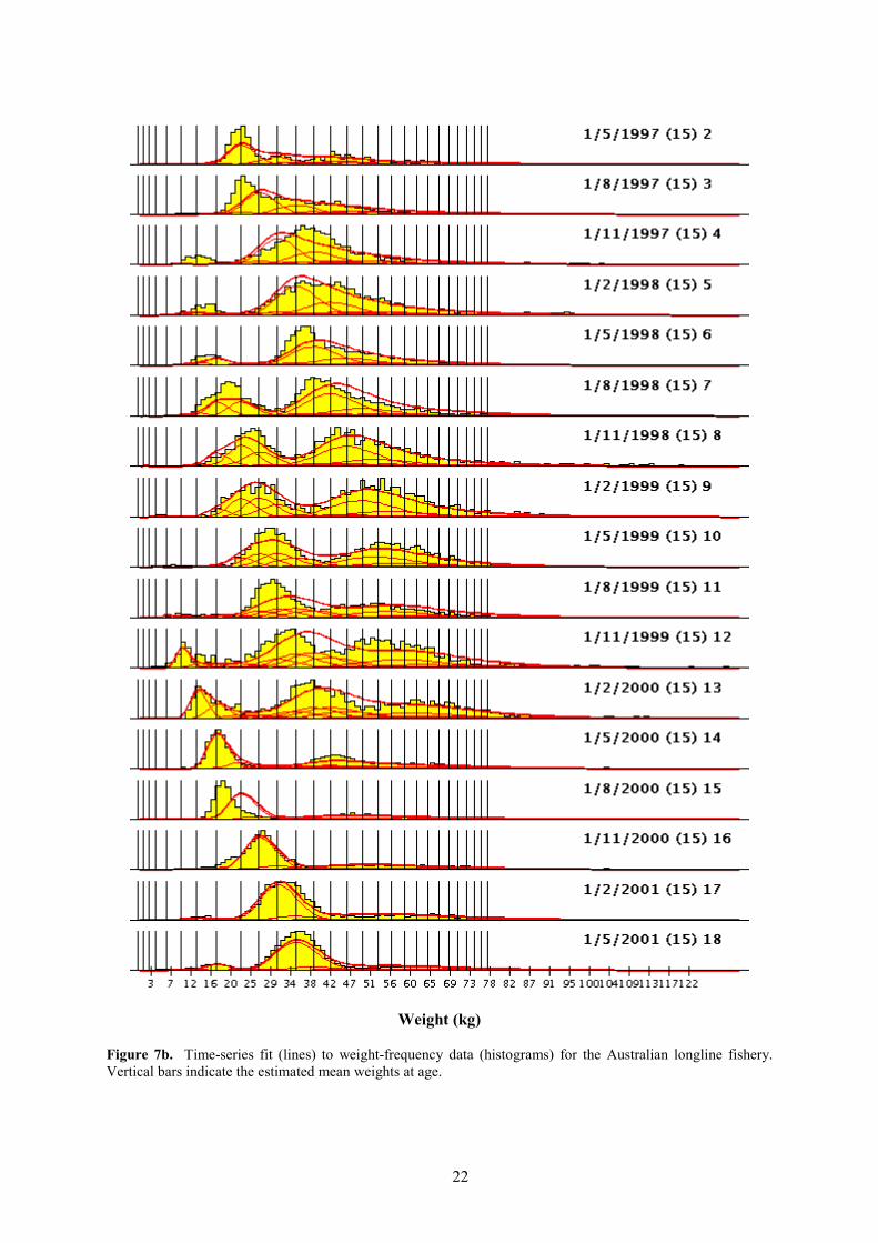
The fit to the weight-frequency data aggregated over time is shown in Figure 7a and anexample of the fits to time-series data (for the Australian longline fishery) is shown in Figure 7b.There is some systematic lack of fit to the data for fisheries LL 2 and LL 3. Length-frequency data arealso available for these fisheries and these data are not always consistent with the weight-frequencydata. This is probably because the weight-frequency data come mainly from Taiwanese longliners inthe case of LL 2 and from Hawaii and Pacific Island longliners in the case of LL 3. In contrast, thelength-frequency data are sourced mainly from Japanese longliners. It is possible that these fleets havedifferent selectivity characteristics, which might cause the inconsistencies in the data sets. This couldbe dealt with in future analyses by defining separate fisheries for the Japanese and other fleetsmentioned.

The fits of the model to the tagging data compiled by calendar time and by time at liberty areshown in Figure 8a and b. The model results are fairly consistent with the aggregate tag-return data,although the predicted returns are generally fewer than observed for the longer times at liberty. Thisdiscrepancy is almost entirely due to an inability of the model to predict the large numbers of returnsrecorded by the Australian longline fishery (Figure 8c). The higher numbers of observed tag returnsfor this fishery indicates an inadequacy of the spatial structure of the model and a failure in thisinstance of the tagged fish mixing assumption. It seems that at least some of the large numbers of tagsreleased in the vicinity of this fishery (off north-eastern Australia at about 16°S) in 1991 and 1992remained in this area and were hence vulnerable to the Australian longline fishery for an extendedperiod. This problem could be remedied by defining an additional model region that more closelyapproximates the area of operation of that component of the Australian longline fleet that returnedthese tags.

8

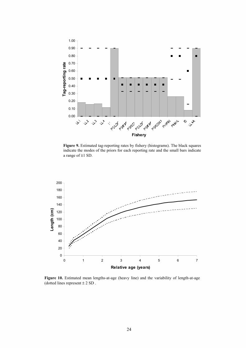
5.2 Tag-reporting ratesEstimated tag-reporting rates by fishery are shown in Figure 9. The estimates for the purse

seine fisheries are all near the modes of their prior distributions. The estimates for the Philippines andIndonesian fisheries are significantly below its prior mode, indicating that the model has usedinformation contained in the data to estimate this reporting rate. The estimates for the longlinefisheries are highly variable, ranging from <0.2 to the upper limit allowed (0.9).

5.3 Age and growthUsing the four-recruitment-per-year formulation, the model was able to detect a coherent

growth signal in the size data. The estimated growth curve is shown in Figure 10. The non-vonBertalanffy growth of juvenile bigeye is clearly evident, with a pronounced reduction in growth ratein the 40−70 cm size range. This growth pattern is similar to that observed in both otolith and tagginglength-increment data (Lehodey et al. 1999).

5.4 SelectivityEstimated selectivity coefficients are generally consistent with expectation (Figure 11). For

the purse seine fisheries, the selectivities are similar for all set types, with a slightly higher tendencyfor school sets to capture large bigeye tuna. There are also similarities among regions in the selectivityestimates for the purse seine fisheries, suggesting that some aggregation of parameters may bepossible in future analyses. Longline selectivity coefficients increase to full recruitment at 2−3 yearsof age.

5.5 CatchabilityTime-series changes in catchability are evident for several fisheries (Figure 12). There is

evidence of strongly increasing catchability in all of the purse seine fisheries.

In this analysis, catchability in the longline fisheries has been assumed to be constant overtime, with the exception of seasonal variation, which is apparent mainly in the North Pacific (LL 1)and South Pacific (LL 4, LL 5) regions.

The overall consistency of the model with the observed effort data can be examined in plotsof effort deviations against time for each fishery (Figure 13). If the model is coherent with the effortdata, we would expect an even scatter of effort deviations about zero. Some outliers would also beexpected, which prompted the use of robust estimation techniques. On the other hand, if there was anobvious trend in the effort deviations with time, this may indicate that a trend in catchability hadoccurred and that this had not been sufficiently captured by the model. No unusual variability in theresiduals is apparent in Figure 13, suggesting that the model has extracted all the information presentin the data regarding catchability variation. In particular, there is no evidence that the assumption ofno time-series or regional variation in catchability for the longline fisheries is inappropriate.

Figure 13 also provides an indication of the relative variability of the effort data with respectto the model. The plots suggest that the data for the LL 2 and LL 3 fisheries (the longline fisheries inthe tropics) are the least variable and may therefore provide the best information on the stockdynamics.

For the LL 1 − LL 5 longline fisheries, we assumed catchability to be constant among regions,as well as over time (with the exception of seasonal variation). This assumption was consideredappropriate because of the use of standardized effort for these fisheries, i.e. the numbers of longlinehooks fishing in bigeye tuna habitat (the upper mixed layer) in a standardized area. Given thisassumption and treatment of the longline effort data, we would expect that longline CPUE wouldprovide an index of exploitable abundance (population-at-age multiplied by age-specific selectivityand summed across age-classes) in each region. Figure 14 compares longline exploitable abundanceand CPUE for each region. There is generally good, though not perfect agreement between the time-

9

series patterns of both variables in each region. This indicates that the model results reflect longlineCPUE as intended by the catchability assumptions.

5.6 Natural mortalityNatural mortality shows considerable variation with size and age-class (Figure 15). For the

mid-sizes of ~50-100 cm, the estimates are in the range 0.07-0.10 qtr-1. Estimates for both smaller andlarger bigeye tuna are higher, giving the M-at-age curve a U-shaped appearance. The right hand end ofthe curve begins its upward movement at around the size at first maturity, peaking at about 140 cm insize. This has been postulated to be due to higher female mortality associated with spawning.

5.7 MovementA representation of the dispersal patterns resulting from the estimated movement parameters

is shown in Figure 16, which shows the changes in the relative distributions over time of cohortsoriginating in each region. Movement patterns in the tropics (regions 2 and 3) imply that netmovement is west to east.

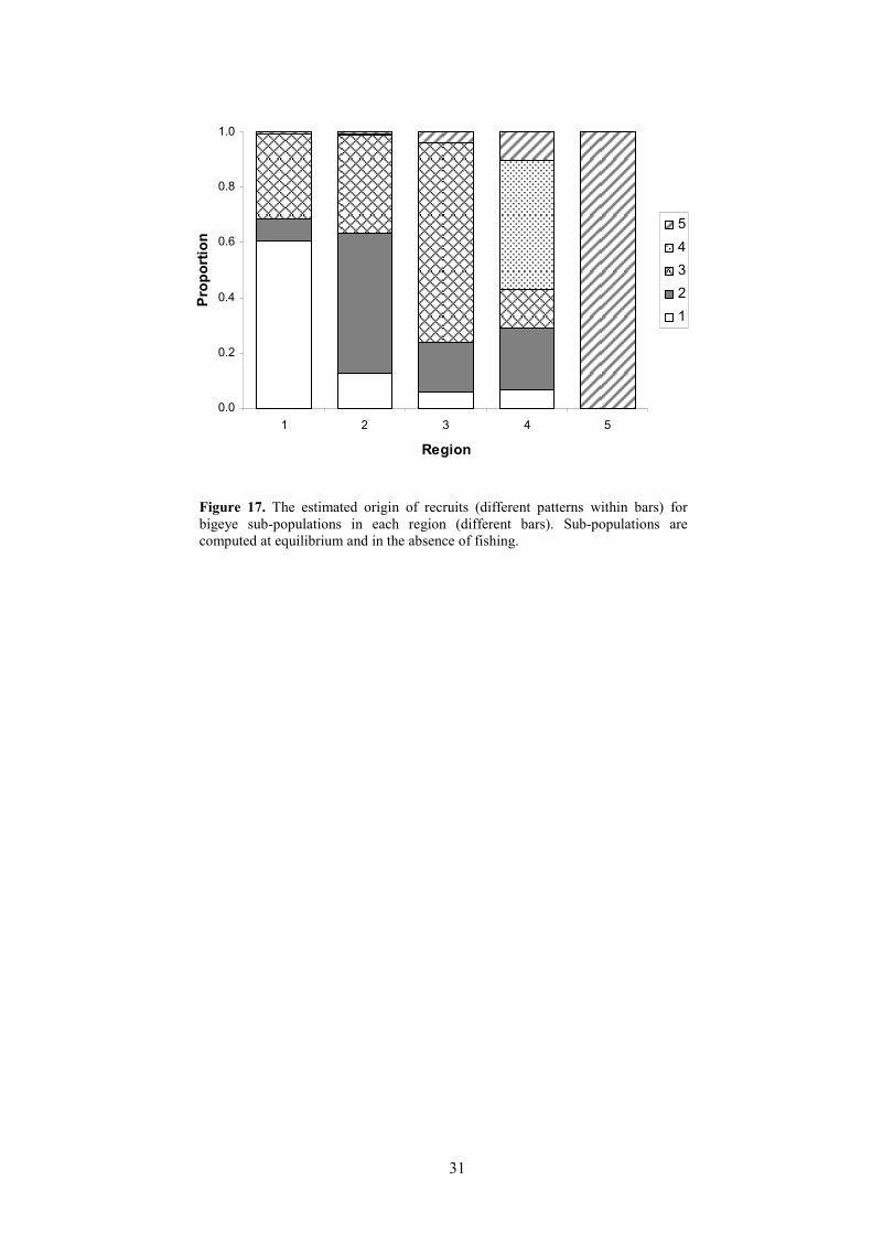
It is also possible to use the movement coefficients, the average proportions of the totalrecruitment occurring in each region and the age-specific natural mortality rates to estimate theequilibrium stock composition in each region in the absence of fishing (Figure 17). The model resultsimply that 61% of the equilibrium biomass in region 1 would be composed of fish recruited in thatregion. The contributions of local recruitment to equilibrium biomass in the other regions is 51%(region 2), 72% (region 3), 47% (region 4) and 100% (region 5).

5.8 RecruitmentThe total recruitment estimates (Figure 18a) are characterised by relative stability over most

of the time series, but with an increase since the mid-1990s. The precision of the total recruitmentestimates is indicated by the approximate 95% confidence intervals (Figure 18b). For the wholeperiod considered by the model, the average recruitment CV is about 0.17. However, the CV is muchhigher towards the end of the time. This degradation in performance of recruitment estimates isexpected for cohorts that have experienced relatively little fishing.

5.9 BiomassTime series of total and adult relative biomass, by region are shown in Figure 19. Relative

total and adult biomass has declined mainly in the tropical regions (2 and 3), resulting in an overalldecline to the mid-1990s. Since then, biomass is estimated to have increased, mainly in region 5, as aresult of high estimated recruitment.

5.10 Fishing mortality and the impact of fishingAverage fishing mortality rates for juvenile and adult age groups are shown in Figure 20 for

the total model area. Fishing mortality for adults has increased steadily over the time series, flatteningout after 1995. In contrast, juvenile fishing mortality has increased rapidly particularly since the early1990s. A major factor in this increase has been the increase in assumed catches in Indonesia, whichare based on yellowfin tuna catches reported by the national authorities in Indonesia, which, in theabsence of sampling data, we assume contain a fixed proportion of bigeye tuna. Increased purse seinecatches, mainly using FAD sets, have also contributed to increased juvenile fishing mortality.

For a complex model such as this, it is difficult to readily interpret fishing mortality rates andother parameters to obtain a clear picture of the estimated impact of fishing on the stock. To facilitatethis, we have computed total biomass trajectories for the population in each region using the estimatedrecruitment, natural mortality and movement parameters, but assuming that the fishing mortality waszero throughout the time series. Comparison of these biomass trajectories with those incorporating the

10

actual levels of observed historical fishing provides a concise, integrated picture of the impacts of thetotal fishery on the stock. Biomass trajectories for each region and for the WCPO in total are shown inFigure 21. The greatest impacts have occurred in regions 2 and 3, where the “actual” biomass is lessthan 50% of the “unfished” biomass. This result would suggest that there has been a significantdepletion of the sub-populations in these regions, primarily by the domestic fisheries of thePhilippines and Indonesia and the combined purse seine fishery. For the WCPO in total, the currentbiomass is estimated to be around 35% less than that which would have occurred in the absence offishing.

5.11 Yield and reference point analysisThe use of reference points provides a framework for quantitatively determining the status of

the stock and its exploitation level. Two types of reference points are often now required for fisheriesmanagement: the fishing mortality at maximum sustainable yield (FMSY) is used as an indicator ofoverfishing; and the biomass at MSY (BMSY) is used as an indicator of an overfished state. It ispossible for overfishing to be occurring, but for the stock to not yet be in an overfished state.Conversely, it is possible for the stock to be in an overfished state but for the current level of fishingto be within the overfishing reference point. In this case, the stock has presumably been depressed bypast overfishing and would recover to a non-overfished state if the current level of fishing wasmaintained. It is likely that these reference points, or something similar, will be used for stock statusdeterminations in the new WCPO tuna commission. We have therefore developed a reference pointanalysis within the MULTIFAN-CL model framework as an example of how this might be applied inWCPO tuna fisheries.

The reference point analysis has been carried out as follows:

1. Estimate population model parameters, including the parameters of a Beverton and Holt stock-recruitment relationship (SRR).

2. Estimate a “base” age-specific fishing mortality vector, Fage, various multiples of which areassumed to maintained into the future; for the bigeye tuna assessment, the average Fage over1996−2000 was used.

3. For various multiples of Fage compute the equilibrium population-at-age, and equilibrium yieldusing the estimated SRR, natural mortality and other parameters.

4. Compute the equilibrium total biomass, equilibrium adult biomass and equilibrium fishingmortality (averaged over age classes) at MSY. These equilibrium quantities are the referencepoints.

5. Compare the actual estimated biomass and fishing mortality levels at time t with these referencepoints. This is done by computing the ratios total

MSYtotalt BB , adult

MSYadultt BB , MSYt FF and their 95%

confidence intervals and comparing them with 1.0. Values of MSYt FF significantly greater than

1.0 would indicate overfishing, while values of totalMSY

totalt BB and/or adult

MSYadultt BB or less than 1.0

would indicate an overfished state.

Note that these somewhat simplistic notions make assumptions about equilibrium behaviourof the populations. This aspect of reference points and in particular those based on equilibrium modelshas been roundly criticised (with some justification) in some fisheries circles. One criticism is thatlong-term changes in recruitment might occur through environmental or ecosystem changes that havelittle or nothing to do with the fisheries. More generally, it is not unreasonable to view many fishpopulations as being in a continual state of flux with an equilibrium condition never being reached ormaintained for any length of time. In reality, therefore, MSY, FMSY and BMSY are “moving targets” andnot static quantities. At best, they should be considered as averages over time, and additional analysesundertaken in cases where it is suspected that important non-fishery-induced changes in productivitymay have occurred.

11

The estimated SRR used in the yield and reference point analyses for bigeye tuna is shown inFigure 22. The scatter of recruitment-biomass points is fairly typical of most fisheries data sets − thereis very little information on how recruitment might respond to very low biomass levels. For thisreason, it is necessary to constrain the behaviour of the curve in the region towards the origin by theprior assumption for “steepness”. To recap, the assumption was that significant (>10%) recruitmentdecline occurs only at adult biomass of <20% of virgin levels, i.e. that average recruitment is quiterobust to adult biomass decline.

The estimated equilibrium yield using a base F-at-age given by the 1996−2000 average isshown in Figure 23. This analysis indicates that, at the 1996−2000 average F-at-age (i.e. a fishingmortality multiplier of 1.0), the equilibrium yield is approximately 75,000 t per year. The maximumequilibrium yield (equivalent to MSY) of about 87,000 t is achieved at a F-multiplier of 1.7. Theseequilibrium yields are considerably lower than the actual catches that occurred during 1996−2000,which averaged about 103,000 t per year. This is because the yield analysis is based on an equilibriummodel in which equilibrium recruitment is predicted on the basis of the SRR shown in Figure 22.However, recruitment during the mid- to late-1990s was at a relatively high level which enabled therecent high catches to occur.

Recruitment effects such as noted above can obviously bias status determinations based on acomparison of catch and MSY. A comparison of F with FMSY is better from this point of view as theeffects of recruitment are removed. The ratios of MSYt FF and adult

MSYadultt BB are shown in Figure 24.

MSYt FF has been beneath the overfishing reference point throughout the time series. Also, while

adult biomass has fallen recently, adultMSY

adultt BB has remained above 1.0, indicating that the

population has yet to reach an overfished state under the definition used here. The recent highrecruitment and increased biomass has moved adult

MSYadultt BB further away from the reference level.

6 ConclusionsThe bigeye tuna model has integrated catch, effort, length-frequency, weight-frequency and

tagging data into a coherent analysis that is broadly consistent with other information on the biologyand fisheries. The major conclusions of the analysis with respect to stock assessment are:

1. Recruitment varies seasonally and interannually, but no persistent trends are evident in the timeseries. Recruitment in the late 1990s was at above-average levels.

2. Bigeye tuna biomass in the WCPO declined to around 60% of its early 1960s level but hasrecently increased as a result of above-average recruitment in the late 1990s.

3. By the late 1990s, the biomass is estimated to have been approximately 35% below the level itwould have been if fishing had never occurred. The impact of the fisheries is differentially high inthe tropical regions (>50%) compared to the subtropical regions.

4. Fishing mortality for juvenile bigeye tuna has increased strongly since about 1992, partly as aresult of catchability increases in the purse seine fisheries. But a significant component of theincrease is attributable to the Philippines and Indonesian fisheries, which have the weakest catch,effort and size data. This is of continuing concern. There has been recent progress made in theacquisition of a large amount of historical length frequency data from the Philippines and regularsampling operations are now in place there. However, uncertainty with the total catch and sizecomposition data for the Indonesian fishery continues to be a problem.

5. While aggregate fishing mortality increased to at least the mid 1990s, MSYt FF has remainedbelow the reference level of 1.0, indicating that overfishing has not yet occurred. Also,

adultMSY

adultt BB has remained significantly above 1.0, indicating that the stock has not yet reached

an overfished state.

12

6. Recommended research and monitoring required to improve the bigeye tuna assessment includethe following:

• Continued monitoring and improvement in fisheries statistics is required. In particular, betterdata generally are required for the Philippines and Indonesian fisheries, and improvedsampling coverage of the purse seine fleet is required to improve the estimates of catch.

• New conventional tagging experiments, undertaken regularly, would provide additionalinformation on recent levels of fishing mortality, refine estimates of natural mortality andpossibly allow some time-series behaviour in movement to be incorporated into the model.

• In view of the importance placed on longline effort data by this model, additional archivaltagging is required to characterise the depth distribution of bigeye tuna and its environmentalcorrelates across the stock range to enable better estimation of effective longline effort.

7 AcknowledgementsWe are grateful to Naozumi Miyabe of the Japan National Research Institute of Far Seas

Fisheries for his assistance in compiling data for the Japanese fisheries.

8 References

Bigelow, K. A., J. Hampton, and N. Miyabe. 2002. Application of a habitat based model to estimateeffective longline fishing effort and relative abundance of Pacific bigeye tuna (Thunnus obesus).Fish. Oceanogr. 11: 143-155.

Brill, R.W., 1994. A review of temperature and oxygen tolerance studies of tunas pertinent to fisheriesoceanography, movement models and stock assessments. Fish. Oceanogr. 3:204−216.

Dagorn, L., Bach, P., and Josse, E. 2000. Movement patterns of large bigeye tuna (Thunnus obesus) inthe open ocean, determined using ultrasonic telemetry. Mar. Biol. 136: 361−371.

Fournier, D.A., Hampton, J., and Sibert, J.R. 1998. MULTIFAN-CL: a length-based, age-structuredmodel for fisheries stock assessment, with application to South Pacific albacore, Thunnusalalunga. Can. J. Fish. Aquat. Sci. 55: 2105−2116.

Francis, R.I.C.C. 1992. Use of risk analysis to assess fishery management strategies: a case studyusing orange roughy (Hoplostethus atlanticus) on the Chatham Rise, New Zealand. Can. J. Fish.Aquat. Sci. 49: 922−930.

Grewe, P.M., and Hampton, J. 1998. An assessment of bigeye (Thunnus obesus) populationstructure in the Pacific Ocean based on mitochondrial DNA and DNA microsatelliteanalysis. SOEST 98-05, JIMAR Contribution 98-330.

Hampton, J. 1997. Estimates of tag-reporting and tag-shedding rates in a large-scale tuna taggingexperiment in the western tropical Pacific Ocean. Fish. Bull. U.S. 95:68−79.

Hampton, J. 2000. Natural mortality rates in tropical tunas: size really does matter. Can. J. Fish.Aquat. Sci. 57: 1002−1010.

Hampton, J., and Fournier, D.A. 2001. A spatially-disaggregated, length-based, age-structuredpopulation model of yellowfin tuna (Thunnus albacares) in the western and central PacificOcean. Mar. Freshw. Res. 52:937−963.

Hampton, J., K. Bigelow, and M. Labelle. 1998. A summary of current information on the biology,fisheries and stock assessment of bigeye tuna (Thunnus obesus) in the Pacific Ocean, withrecommendations for data requirements and future research. Technical Report No. 36, (OceanicFisheries Programme Secretariat of the Pacific Community, Noumea, New Caledonia) 46 pp.

13

Kaltongga, B. 1998. Regional Tuna Tagging Project: data summary. Technical Report No. 35,(Oceanic Fisheries Programme, Secretariat of the Pacific Community, Noumea, NewCaledonia.) 70 pp.

Lehodey, P., Hampton, J., and B. Leroy. 1999. Preliminary results on age and growth of bigeye tuna(Thunnus obesus) from the western and central Pacific Ocean as indicated by daily growthincrements and tagging data. Working Paper BET-2, 12th meeting of the Standing Committeeon Tuna and Billfish, Papeete, French Polynesia, 16 −23 June 1999.

Maunder, M.N., and Watters, G.M. 2001. A-SCALA: An age-structured statistical catch-at-lengthanalysis for assessing tuna stocks in the eastern Pacific Ocean. Background Paper A24, 2nd

meeting of the Scientific Working Group, Inter-American Tropical Tuna Commission, 30 April− 4 May 2001, La Jolla, California.

OFP. 2002. Overview of bigeye in western and central Pacific Ocean (WCPO) tuna fisheries. PaperABY5/WP1.1 Part 1, ABY Working Group of the Forum Fisheries Committee (FFC), 3 May2002, Pohnpei, Federated States of Micronesia.

14

Table 1. Definition of fisheries for the MULTIFAN-CL analysis of bigeye tuna.

Fishery Nationality Gear Region

LL 1 All Longline 1

LL 2 All Longline 2

LL 3 All Longline 3

LL 4 All excl. Australia Longline 4

LL 4A Australia Longline 4

LL 5 All Longline 5

PS/LOG 2 All Purse seine, log sets 2

PS/FAD 2 All Purse seine, FAD sets 2

PS/SCH 2 All Purse seine, school sets 2

PS/LOG 3 All Purse seine, log sets 3

PS/FAD 3 All Purse seine, FAD sets 3

PS/SCH 3 All Purse seine, school sets 3

PH/R 3 Philippines Ringnet 2

PH/H 3 Philippines Handline 2

ID 3 Indonesia Various 2

15

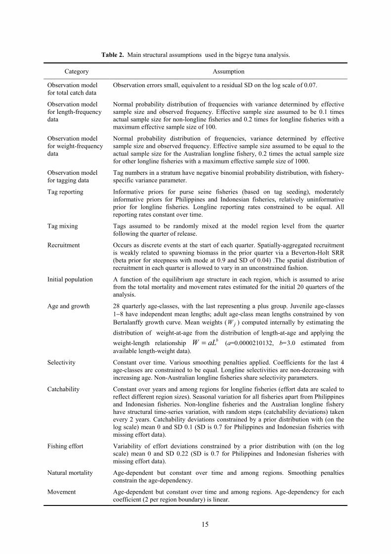
Table 2. Main structural assumptions used in the bigeye tuna analysis.

Category Assumption

Observation modelfor total catch data

Observation errors small, equivalent to a residual SD on the log scale of 0.07.

Observation modelfor length-frequencydata

Normal probability distribution of frequencies with variance determined by effectivesample size and observed frequency. Effective sample size assumed to be 0.1 timesactual sample size for non-longline fisheries and 0.2 times for longline fisheries with amaximum effective sample size of 100.

Observation modelfor weight-frequencydata

Normal probability distribution of frequencies, variance determined by effectivesample size and observed frequency. Effective sample size assumed to be equal to theactual sample size for the Australian longline fishery, 0.2 times the actual sample sizefor other longline fisheries with a maximum effective sample size of 1000.

Observation modelfor tagging data

Tag numbers in a stratum have negative binomial probability distribution, with fishery-specific variance parameter.

Tag reporting Informative priors for purse seine fisheries (based on tag seeding), moderatelyinformative priors for Philippines and Indonesian fisheries, relatively uninformativeprior for longline fisheries. Longline reporting rates constrained to be equal. Allreporting rates constant over time.

Tag mixing Tags assumed to be randomly mixed at the model region level from the quarterfollowing the quarter of release.

Recruitment Occurs as discrete events at the start of each quarter. Spatially-aggregated recruitmentis weakly related to spawning biomass in the prior quarter via a Beverton-Holt SRR(beta prior for steepness with mode at 0.9 and SD of 0.04) .The spatial distribution ofrecruitment in each quarter is allowed to vary in an unconstrained fashion.

Initial population A function of the equilibrium age structure in each region, which is assumed to arisefrom the total mortality and movement rates estimated for the initial 20 quarters of theanalysis.

Age and growth 28 quarterly age-classes, with the last representing a plus group. Juvenile age-classes1−8 have independent mean lengths; adult age-class mean lengths constrained by vonBertalanffy growth curve. Mean weights ( jW ) computed internally by estimating thedistribution of weight-at-age from the distribution of length-at-age and applying theweight-length relationship baLW = (a=0.0000210132, b=3.0 estimated fromavailable length-weight data).

Selectivity Constant over time. Various smoothing penalties applied. Coefficients for the last 4age-classes are constrained to be equal. Longline selectivities are non-decreasing withincreasing age. Non-Australian longline fisheries share selectivity parameters.

Catchability Constant over years and among regions for longline fisheries (effort data are scaled toreflect different region sizes). Seasonal variation for all fisheries apart from Philippinesand Indonesian fisheries. Non-longline fisheries and the Australian longline fisheryhave structural time-series variation, with random steps (catchability deviations) takenevery 2 years. Catchability deviations constrained by a prior distribution with (on thelog scale) mean 0 and SD 0.1 (SD is 0.7 for Philippines and Indonesian fisheries withmissing effort data).

Fishing effort Variability of effort deviations constrained by a prior distribution with (on the logscale) mean 0 and SD 0.22 (SD is 0.7 for Philippines and Indonesian fisheries withmissing effort data).

Natural mortality Age-dependent but constant over time and among regions. Smoothing penaltiesconstrain the age-dependency.

Movement Age-dependent but constant over time and among regions. Age-dependency for eachcoefficient (2 per region boundary) is linear.

16

1

2 3

54

10N

20N

30N

40N

20S

10S

0

120E

40S

30S

120E 130E 140E

130E 140E

150E 160E 170E

150E 160E 170E

180 170W 160W

180 170W 160W

150W 140W 130W

150W 140W 130W 120W 110W 100W

120W 110W 100W 90W 80W

90W 80W

40S30S

10N20N

30N40N

20S10S

0

Figure 1. Long-distance (>1,000 nmi) movements of tagged bigeye tuna. The numbered areas indicate thespatial stratification used in the MULTIFAN-CL model.

0

20,000

40,000

60,000

80,000

100,000

120,000

1960 1964 1968 1972 1976 1980 1984 1988 1992 1996 2000

Catc

h (t)

Other

Purse seine

Longline

Figure 2. WCPO bigeye tuna catch, by gear.

17

10N

20N

30N

40N

20S

10S

0

120E

40S

30S

120E 130E 140E

130E 140E

150E 160E 170E

150E 160E 170E 180 170W 160W

180 170W 160W 150W

150W

40S30S

10N20N

30N40N

20S10S

0

1

2 3

4 5Bigeye catch1996-2000

20,00010,0002,000

LonglinePurse seineOther

Figure 3. Distribution of bigeye tuna catch, 1996−2000. The numbered areas indicatethe spatial stratification used in the MULTIFAN-CL model.

18

0

5

10

15

20

25

30

1960 1970 1980 1990 2000

LL 1

0

5

10

15

20

25

30

1960 1970 1980 1990 2000

LL 2

0

5

10

15

20

25

30

1960 1970 1980 1990 2000

LL 3

0

5

10

15

20

25

30

1960 1970 1980 1990 2000

LL 4

0

5

10

15

20

25

30

1960 1970 1980 1990 2000

LL 5

0.0

0.5

1.0

1.5

2.0

2.5

3.0

1960 1970 1980 1990 2000

PS LOG 2

0.0

0.1

0.2

0.3

0.4

0.5

0.6

1960 1970 1980 1990 2000

LL 4A

0.0

0.5

1.0

1.5

2.0

2.5

3.0

1960 1970 1980 1990 2000

PS FAD 2

0.0

0.5

1.0

1.5

2.0

2.5

3.0

1960 1970 1980 1990 2000

PS SCH 2

0.0

0.5

1.0

1.5

2.0

2.5

3.0

1960 1970 1980 1990 2000

PS LOG 3

0.0

0.5

1.0

1.5

2.0

2.5

3.0

1960 1970 1980 1990 2000

PS FAD 3

0.0

0.5

1.0

1.5

2.0

2.5

3.0

1960 1970 1980 1990 2000

PS SCH 3

Figure 4. Catch per unit effort by fishery. Units are catch number per 100 hooks fishing in bigeye tuna habitat(fisheries LL1, LL2, LL3, LL4, LL5), catch number per 100 nominal hooks (LL4A) and catch (t) per dayfished/searched (all PS fisheries).

19

0.0E

+00

1.0E

+05

2.0E

+05

3.0E

+05

LL 1

0.0E

+00

5.0E

+04

1.0E

+05

1.5E

+05

LL 2

0.0E

+00

2.0E

+05

4.0E

+05

6.0E

+05

LL 3

0.0E

+00

1.0E

+04

2.0E

+04

3.0E

+04

LL 4

0.0E

+00

5.0E

+03

1.0E

+04

PS/F

AD

3

0.0E

+00

2.0E

+02

4.0E

+02

6.0E

+02

PS/S

CH 3

0.0E

+00

5.0E

+02

1.0E

+03

PS/R

3

0.0E

+00

5.0E

+02

1.0E

+03

1.5E

+03

PH/H

3

0.0E

+00

2.0E

+04

4.0E

+04

6.0E

+04

8.0E

+04 19

6019

7019

8019

9020

00

LL 5

0.0E

+00

2.0E

+03

4.0E

+03

PS/L

OG

2

0.0E

+00

5.0E

+02

1.0E

+03

1.5E

+03

PS/F

AD

2

0.0E

+00

1.0E

+03

2.0E

+03

3.0E

+03

4.0E

+03 19

6019

7019

8019

9020

00

ID 3

0.0E

+00

5.0E

+03

1.0E

+04

1.5E

+04

LL 4

A

0.0E

+00

2.0E

+02

4.0E

+02

6.0E

+02

PS/S

CH 2

Catch (t or numbers of fish)

0.0E

+00

2.0E

+03

4.0E

+03

6.0E

+03 19

6019

7019

8019

9020

00

PS/L

OG

3

Figu

re 5

. O

bser

ved

(circ

les)

and

pre

dict

ed (l

ines

) tot

al c

atch

es b

y fis

hery

and

qua

rter.

Cat

ches

are

in to

nnes

for a

ll fis

herie

s ex

cept

the

long

line

(LL)

fish

erie

s, w

here

the

catc

hes a

re in

num

ber o

f fis

h.

20

LL 1

LL 2

LL 3

LL 4

LL 5

PS/LOG 2

PS/FAD 2

PS/SCH 2

PS/LOG 3

PS/FAD 3

PS/SCH 3

PH/R 2

PH/H 2

ID 2

LL 4A No data

Length (cm)

Figure 6. Observed (histograms) and predicted (line) length frequencies for each fishery aggregated over time.

21

LL 1

LL 2

LL 3

LL 4

LL 5

PS/LOG 2

PS/FAD 2

PS/SCH 2

PS/LOG 3

PS/FAD 3

PS/SCH 3

PH/R 2

PH/H 2

ID 2

LL 4A

No data

No data

No data

No data

No data

No data

No data

No data

No data

No data

No data

Weight (kg)

Figure 7a. Observed (histograms) and predicted (line) weight frequencies for each fishery aggregated overtime.

22

Weight (kg)

Figure 7b. Time-series fit (lines) to weight-frequency data (histograms) for the Australian longline fishery.Vertical bars indicate the estimated mean weights at age.

23

0

1

10

100

1,000

1 3 5 7 9 11 13 15 17 19 21 23 25 27 29 31 33 35 37 39 41 43 45Periods at liberty

b

0

100

200

300

1988 1990 1992 1994 1996 1998 2000 2002Recapture period

Predicted

Observed

a

0

5

10

15 cLongline

0

20

40

60PS 2

010203040

PS 3

0

100

200

300PH

0

2

4

6

1988 1990 1992 1994 1996 1998 2000 2002

ID

010203040

Australianlongline

Num

ber o

f tag

retu

rns

Figure 8. Observed (circles) and predicted (lines) tag returns (a) totals byrecapture period, (b) totals by time at liberty, and (c) by various fisherygroupings.

24

0.00

0.10

0.20

0.30

0.40

0.50

0.60

0.70

0.80

0.90

1.00

Fishery

Tag-

repo

rting

rate

Figure 9. Estimated tag-reporting rates by fishery (histograms). The black squaresindicate the modes of the priors for each reporting rate and the small bars indicatea range of ±1 SD.

0

20

40

60

80

100

120

140

160

180

200

0 1 2 3 4 5 6 7

Relative age (years)

Leng

th (c

m)

Figure 10. Estimated mean lengths-at-age (heavy line) and the variability of length-at-age(dotted lines represent ± 2 SD .

25

Sele

ctiv

ity c

oeffi

cien

t

0.0

0.5

1.0 LL 1-5

0.0

0.5

1.0 LL 4A

0.0

0.5

1.0 PS LOG 2

0.0

0.5

1.0 PS FAD 2

0.0

0.5

1.0 PS SCH 2

0.0

0.5

1.0 PS LOG 3

0.0

0.5

1.0 PS FAD 3

0.00.51.0

1 3 5 7 9 11 13 15 17 19 21 23 25 27

Quarterly age class

ID

0.0

0.5

1.0 PS SCH 3

0.0

0.5

1.0 PH/R

0.0

0.5

1.0 PH/H

Figure 11. Selectivity coefficients, by fishery.

26

0.E+

00

1.E-

02

2.E-

02LL

1

0.E+

00

1.E-

02

2.E-

02LL

2

0.E+

00

1.E-

02

2.E-

02LL

3

0.E+

00

1.E-

02

2.E-

02LL

4

0.E+

00

5.E-

03

1.E-

02PS

/FA

D 3

0.E+

00

5.E-

03

1.E-

02

1960

1970

1980

1990

2000

PS/L

OG

3

0.E+

00

5.E-

04PS

/SCH

3

0.E+

00

5.E-

03

1.E-

02PH

/R

0.E+

00

1.E-

02

2.E-

02PH

/H

0.E+

00

1.E-

02

2.E-

02

1960

1970

1980

1990

2000

LL 5

0.E+

002.

E-02

4.E-

026.

E-02

1960

1970

1980

1990

2000

ID

Catchability coefficient

0.E+

00

2.E-

02

4.E-

02PS

/LO

G 2

0.E+

00

1.E-

02

2.E-

02PS

/FA

D 2

0.E+

00

1.E-

03

2.E-

03PS

/SCH

2

0.E+

00

5.E-

04

1.E-

03LL

4A

Figu

re 1

2.

Estim

ated

cat

chab

ility

tren

ds fo

r eac

h fis

hery

.

27

-2-1012LL

1

-2-1012LL

2

-2-1012LL

3

-2-1012LL

4

-2-1012LL

5

-4-2024PS

/LO

G 2

-4-2024PS

/FA

D 3

-4-2024PS

/SCH

3

-101PH

/R

-101PH

/H

-101ID

-4-2024PS

/FA

D 2

-4-2024PS

/SCH

2

-4-2024PS

/LO

G 3

Effort residuals

-2-1012LL

4A

Figu

re 1

3. E

ffort

devi

atio

ns b

y tim

e pe

riod

for e

ach

fishe

ry. T

he X

-axi

s sca

le is

196

2−20

02. T

he Y

-axi

s sca

le is

in S

D u

nits

.

28

0.0

0.5

1.0

1.5

2.0

2.5Region 1

0.0

0.5

1.0

1.5

2.0 Region 2

0.0

0.5

1.0

1.5

2.0

2.5Region 3

0.0

0.5

1.0

1.5

2.0

2.5Region 4

0.0

0.5

1.0

1.5

2.0

2.5

1960 1970 1980 1990 2000

Region 5

Rela

tive

CPUE

and

exp

loita

ble

abun

danc

e

Figure 14. Estimates of exploitable abundance (solid lines) and CPUE(dashed lines) for the longline fisheries in each region. Both variableshave been smoothed to remove seasonal variation and are scaled relativeto their averages.

29

0.00

0.05

0.10

0.15

0.20

0.25

20 40 60 80 100 120 140 160

Mean length-at-age (cm)

Natu

ral m

orta

lity

rate

(per

qua

rter)

Figure 15. Estimated natural mortality rate by age-class plotted against meanlength-at-age with 95% confidence intervals.

30

0

200

400

600

800

1000 Region 5Region 4Region 3

Region 2Region 1Region 1 recruits

0

200

400

600

800

1000

Region 2 recruits

0

200

400

600

800

1000

Region 3 recruits

0

200

400

600

800

1000

Region 4 recruits

0

200

400

600

800

1000

1 3 5 7 9 11 13 15 17 19 21 23 25 27 29 31 33 35 37 39 41

Time (quarters)

Region 5 recruits

Figure 16. Relative distributions over time of cohorts recruited ineach region.

31

0.0

0.2

0.4

0.6

0.8

1.0

1 2 3 4 5

Region

Prop

ortio

n54321

Figure 17. The estimated origin of recruits (different patterns within bars) forbigeye sub-populations in each region (different bars). Sub-populations arecomputed at equilibrium and in the absence of fishing.

32

0.0

1.0

2.0

3.0

4.0

5.0Total WCPO b

0.0

0.5

1.0

1.5

2.0Region 1 c

0.0

0.5

1.0Region 2

0.0

0.5

1.0

1.5Region 3

0.0

0.2

0.4

0.6Region 4

0.00.20.40.60.81.01.2

1960 1965 1970 1975 1980 1985 1990 1995 2000

Region 5

Rela

tive

recr

uitm

ent

0.00.51.01.52.02.53.0

Total WCPOa

Figure 18. Time-series of estimated bigeye tuna recruitment for the base-case model: (a)quarterly recruitment estimates (circles) and moving 4-quarter average spatially-aggregated recruitment (heavy line); (b) 95% confidence intervals for quarterlyrecruitment; and (c) quarterly recruitment estimates by region (circles) and 4-quartermoving averages (heavy lines).

33

0.0

0.2

0.4

0.6

0.8

1.0

1.2

1.4

1962 1966 1970 1974 1978 1982 1986 1990 1994 1998

Rela

tive

tota

l bio

mas

s

Region 5

Region 4

Region 3

Region 2

Region 1

a

0.0

0.2

0.4

0.6

0.8

1.0

1.2

1.4

1962 1966 1970 1974 1978 1982 1986 1990 1994 1998

Rela

tive

adul

t bio

mas

s

Region 5

Region 4

Region 3

Region 2

Region 1

b

Figure 19. Estimated relative total (a) and adult (b) bigeye tuna biomass byregion, and total biomass with 95% confidence intervals (c) for the base-casemodel.

0.00

0.10

0.20

0.30

0.40

1960 1965 1970 1975 1980 1985 1990 1995 2000

Fish

ing

mor

talit

y (p

er y

ear)

Juvenile

Adult

Figure 20. Estimated annual average fishing mortality rates for the WCPO.

34

0.0

0.2

0.4

0.6

0.8

1.0

1.2

1.4

1960 1965 1970 1975 1980 1985 1990 1995 2000

Bio

mas

s in

dex

0

10

20

30

40

50

60

70

% b

iom

ass

redu

ctio

n

a

0.0

0.5

1.0

1.5 Region 1 b

0.0

0.5

1.0

1.5 Region 2

0.0

0.5

1.0

1.5 Region 3

0.0

1.0

2.0

3.0 Region 4

0.0

1.0

2.0

3.0

1960 1970 1980 1990 2000

Region 5

Figure 21. Comparison of the estimated biomass trajectories (lower heavy lines) withbiomass trajectories that would have occurred in the absence of fishing (upper thin lines)for the base-case model. (a) For the WCPO (with the percentage difference in thetrajectories also plotted in grey), and (b) for each region.

35

0.0

0.2

0.4

0.6

0.8

1.0

0.0 0.2 0.4 0.6 0.8 1.0

Relative adult biomass

Rela

tive

recr

uitm

ent

Figure 22. Spawning biomass − recruitment estimates (on a relative scale) and the fittedBeverton and Holt stock-recruitment relationship (SRR) incorporating a prior on steepness of0.9. The dashed lines are the 95% confidence intervals on the SRR.

0

20,000

40,000

60,000

80,000

100,000

120,000

0 1 2 3 4 5 6 7

Fishing mortality multiplier

Equi

libriu

m a

nnua

l yie

ld (t

)

Base F = 1996-2000 average

Figure 23. Predicted equilibrium yield and 95% confidence intervals as a function of fishingmortality (relative to the average fishing mortality-at-age during 1996-2000).

36

0.0

0.2

0.4

0.6

0.8

1.0

1.2

1960 1970 1980 1990 2000

F/F M

SY

a

0

1

2

3

4

5

1960 1970 1980 1990 2000

Adu

lt B

/ A

dult

B MS

Y

b

Figure 24. Ratios of (a) MSYt FF and (b) adultMSY

adultt BB with 95% confidence

intervals. The horizontal lines at 1.0 in each case indicate the overfishing (A) andoverfished state (B) reference points.