BEST PRACTICES IN STRUCTURAL EQUATION …...488 32 BEST PRACTICES IN STRUCTURAL EQUATION MODELING RALPH O. MUELLER GREGORY R. HANCOCK S tructural equation modeling (SEM) has evolved

488

32BEST PRACTICES IN STRUCTURAL

EQUATION MODELING

RALPH O. MUELLER

GREGORY R. HANCOCK

Structural equation modeling (SEM) hasevolved into a mature and popularmethodology to investigate theory-derived

structural/causal hypotheses. Indeed, with thecontinued development of SEM software pack-ages such as AMOS (Arbuckle, 2007), EQS(Bentler, 2006), LISREL (Jöreskog & Sörbom,2006), and Mplus (Muthén & Muthén, 2006),SEM “has become the preeminent multivariatemethod of data analysis” (Hershberger, 2003,pp. 43–44). Yet, we believe that many practitionersstill have little, if any, formal SEM background,potentially leading to misapplications and pub-lications of questionable utility. Drawing on ourown experiences as authors and reviewers ofSEM studies, as well as on existing guides forreporting SEM results (e.g., Boomsma, 2000;Hoyle & Panter, 1995; McDonald & Ho, 2002),we offer a collection of best practices guidelinesto those analysts and authors who contemplate

using SEM to help answer their substantiveresearch questions. Throughout, we assume thatreaders have at least some familiarity with thegoals and language of SEM as covered in anyintroductory textbook (e.g., Byrne, 1998, 2001,2006; Kline, 2005; Loehlin, 2004; Mueller, 1996;Schumacker & Lomax, 2004). For those desiringeven more in-depth or advanced knowledge, werecommend Bollen (1989), Kaplan (2000), orHancock and Mueller (2006).

SETTING THE STAGE

The foundations of SEM are rooted in classicalmeasured variable path analysis (e.g., Wright,1918) and confirmatory factor analysis (e.g.,Jöreskog, 1966, 1967). From a purely statisticalperspective, traditional data analytical techniquessuch as the analysis of variance, the analysis of

Authors’ Note: During the writing of this chapter, the first author was on sabbatical leave from The George Washington

University and was partially supported by its Center for the Study of Language and Education and the Institute for Education

Studies, both in the Graduate School of Education and Human Development. While on leave, he was visiting professor in the

Department of Measurement, Statistics and Evaluation (EDMS) at the University of Maryland, College Park, and visiting

scholar in its Center for Integrated Latent Variable Research (CILVR). He thanks the EDMS and CILVR faculty and staff for

their hospitality, generosity, and collegiality. Portions of this chapter were adapted from a presentation by the authors at the

2004 meeting of the American Educational Research Association in San Diego.

32-Osborne (Best)-45409.qxd 10/9/2007 1:00 PM Page 488

Structural Equation Modeling 489

covariance, multiple linear regression, canonicalcorrelation, and exploratory factor analysis—aswell as measured variable path and confirmatoryfactor analysis—can be regarded as special casesof SEM. However, classical path- and factor-ana-lytic techniques have historically emphasized anexplicit link to a theoretically conceptualizedunderlying causal model and hence are moststrongly identified with the more general SEMframework. Simply put, SEM defines a set ofdata analysis tools that allows for the testing oftheoretically derived and a priori specified causalhypotheses.

Many contemporary treatments introduceSEM not just as a statistical technique but as aprocess involving several stages: (a) initial modelconceptualization, (b) parameter identificationand estimation, (c) data-model fit assessment,and (d) potential model modification. As anystudy using SEM should address these fourstages (e.g., Mueller, 1997), we provide briefdescriptions here and subsequently use them asa framework for our best practices analysis illus-trations and publication guidelines.

Initial Model Conceptualization

The first stage of any SEM analysis shouldconsist of developing a thorough understandingof, and justification for, the underlying theory ortheories that gave rise to the particular model(s)being investigated. In most of the traditionaland typical SEM applications, the operational-ized theories assume one of three forms:

• A measured variable path analysis (MVPA)model: hypothesized structural/causalrelations among directly measured variables;the four-stage SEM process applied to MVPAmodels was illustrated in, for example,Hancock & Mueller, 2004.

• A confirmatory factor analysis (CFA) model:structural/causal relations betweenunobserved latent factors and their measuredindicators; the four-stage SEM process appliedto CFA models was illustrated in, for example,Mueller & Hancock, 2001.

• A latent variable path analysis (LVPA) model:structural/causal relations among latentfactors. This type of SEM model is the focusin this chapter and constitutes a combinationof the previous two. A distinction is madebetween the structural and the measurement

portions of the model: While the former isconcerned with causal relations among latentconstructs and typically is the focus in LVPAstudies, the latter specifies how theseconstructs are modeled using measuredindicator variables (i.e., a CFA model).

More complex models (e.g., multisample,latent means, latent growth, multilevel, or mix-ture models) with their own specific recommen-dations certainly exist but are beyond thepresent scope. Regardless of model type, how-ever, a lack of consonance between model andunderlying theory will have negative repercus-sions for the entire SEM process. Hence, metic-ulous attention to theoretical detail cannot beoveremphasized.

Parameter Identification and Estimation

A model’s hypothesized structural and non-structural relations can be expressed as popula-tion parameters that convey both magnitudeand sign of those relations. Before sample esti-mates of these parameters can be obtained, eachparameter—and hence the whole model—mustbe shown to be identified; that is, it must be pos-sible to express each parameter as a function ofthe variances and covariances of the measuredvariables. Even though this is difficult and cum-bersome to demonstrate, fortunately, the identi-fication status of a model can often be assessedby comparing the total number of parameters to be estimated, t, with the number of unique(co)variances of measured variables,

where p is the total number of measured vari-ables in the model. When t > u (i.e., whenattempting to estimate more parameters thanthere are unique variances and covariances), themodel is underidentified, and estimation ofsome (if not all) parameters is impossible. Onthe other hand, t ≤ u is a necessary but not suf-ficient condition for identification, and usuallyparameter estimation can commence: t = uimplies that the model is justidentified, while t < u implies that it is overidentified (providedthat indeed all parameters are identified and anylatent variables in the system have been assignedan appropriate metric; see Note 4).

u = p(p + 1

)/2,


490 BEST ADVANCED PRACTICES IN QUANTITATIVE METHODS

SEM software packages offer a variety ofparameter estimation techniques for modelswhose identification can be established. Themost popular estimation method (and thedefault in most SEM software packages) is max-imum likelihood (ML), an iterative large-sampletechnique that assumes underlying multivariatenormality. Alternative techniques exist (e.g.,generalized least squares [GLS], asymptoticallydistribution free [ADF; Browne, 1984], androbust estimators [Satorra & Bentler, 1994]),some of which do not depend on a particularunderlying distribution of the data, but still, thevast majority of substantive studies use ML.

Data-Model Fit Assessment

A central issue addressed by SEM is how toassess the fit between observed data and thehypothesized model, ideally operationalized asan evaluation of the degree of discrepancybetween the true population covariance matrixand that implied by the model’s structural andnonstructural parameters. As the populationparameter values are seldom known, the differ-ence between an observed, sample-based covari-ance matrix and that implied by parameterestimates must serve to approximate the popula-tion discrepancy. For a justidentified model, theobserved data will fit the model perfectly: Thesystem of equations expressing each model param-eter as a function of the observed (co)variances isuniquely solvable; thus, the sample estimate ofthe model-implied covariance matrix will, bydefault, equal the sample estimate of the popula-tion covariance matrix. However, if a model isoveridentified, it is unlikely that these two matri-ces are equal as the system of equations (express-ing model parameters as functions of observedvariances and covariances) is solvable in morethan a single way.

Abiding by a general desire for parsimony,overidentified models tend to be of more sub-stantive interest than justidentified ones becausethey represent simpler potential explanations ofthe observed associations. While data-model fitfor such models was initially conceived as a for-mal statistical test of the discrepancy between thetrue and model-implied covariance matrices (achi-square test with df = u–t; Jöreskog, 1966,1967), such a test now is often viewed as overlystrict given its power to detect even trivial devia-tions of a proposed model from reality. Hence,many alternative assessment strategies have

emerged (for a now classic review, see Tanaka,1993) and continue to be developed. Data-modelfit indices for such assessment can be categorizedroughly into three broad classes (with recom-mended indices in italics):

• Absolute indices evaluate the overall dis-crepancy between observed and implied covari-ance matrices; fit improves as more parametersare added to the model and degrees of freedomdecrease: for example, the standardized rootmean square residual (SRMR), the chi-square test(recommended to be reported mostly for its his-torical significance), and the goodness-of-fitindex (GFI).

• Parsimonious indices evaluate the overalldiscrepancy between observed and impliedcovariance matrices while taking into account amodel’s complexity; fit improves as more param-eters are added to the model, as long as thoseparameters are making a useful contribution: forexample, the root mean square error of approxima-tion (RMSEA) with its associated confidenceinterval, the Akaike information criterion (AIC)for fit comparisons across nonnested models, andthe adjusted goodness-of-fit index (AGFI).

• Incremental indices assess absolute or parsi-monious fit relative to a baseline model, usuallythe null model (a model that specifies no relationsamong measured variables): for example, thecomparative fit index (CFI), the normed fit index(NFI), and the nonnormed fit index (NNFI).

If, after considering several indices, data-model fit is deemed acceptable (and judged bestcompared to competing models, if applicable),the model is retained as tenable, and individualparameters may be interpreted. If, however, evi-dence suggests unacceptable data-model fit, thenext and often final stage in the SEM process is considered: modifying the model to improvefit in hopes of also improving the model’s corre-spondence to reality.

Potential Model Modification

In a strict sense, any hypothesized model is, at best, only an approximation to reality; theremaining question is one of degree of that mis-specification. With regard to external specificationerrors—when irrelevant variables were included inthe model or substantively important ones were leftout—remediation can only occur by respecifying



the model based on more relevant theory. On theother hand, internal specification errors—whenunimportant paths among variables were includedor when important paths were omitted—canpotentially be diagnosed and remedied using Waldstatistics (predicted increase in chi-square if a previ-ously estimated parameter were fixed to someknown value, e.g., zero) and Lagrange multiplierstatistics (also referred to as modification indices;estimated decrease in chi-square if a previouslyfixed parameter were to be estimated). As thesetests’ recommendations are directly motivated bythe data and not by theoretical considerations, anyresulting respecifications must be viewed asexploratory in nature and might not lead to amodel that resembles reality any more closely thanthe one(s) initially conceptualized.

BEST PRACTICES IN SEM DATA

ANALYSIS: A SET OF ILLUSTRATIONS

Using the four-stage SEM process as a frame-work, we turn to an illustration of best practicesin the most common type of SEM analyses. Wechose to focus on a set of hypothesized modelsinvolving structural/causal relations amonglatent factors (i.e., LVPA models) to demonstrateour preference for using a two-phase approach(i.e., a measurement phase followed by a struc-tural phase) over a single-phase, all-in-oneanalysis. We conclude this section by illustratingthe statistical comparison of hierarchicallyrelated or nested models (occurring, for example,when one model’s parameters are a proper sub-set of another model’s parameters) and address-ing the disattenuation (i.e., purification andstrengthening) of structural parameter esti-mates obtained from an LVPA when comparedwith those obtained from an analysis of thesame overall structure but one that uses mea-sured variables only.

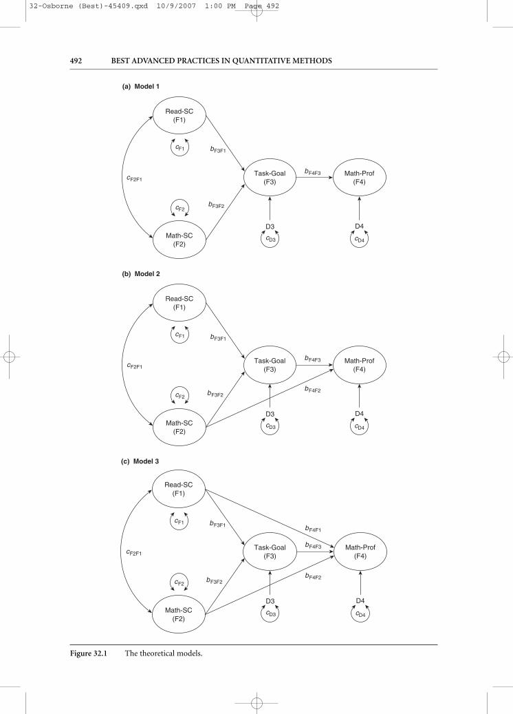
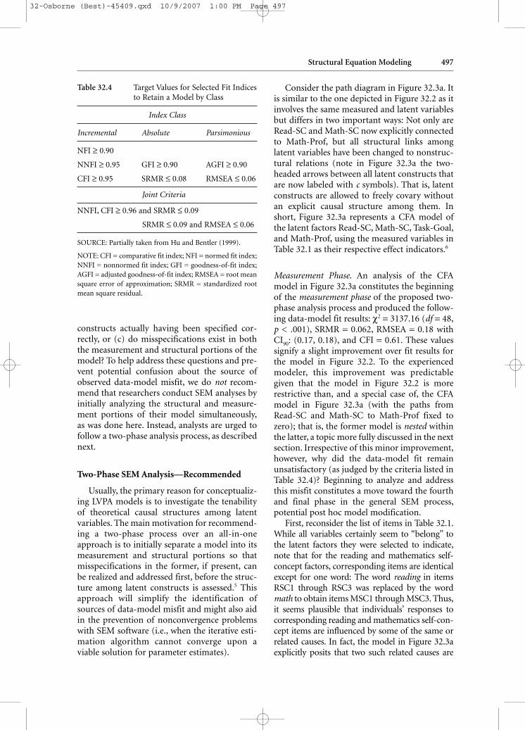
Suppose an educational researcher is inter-ested in investigating the structural effects ofgirls’ reading and mathematics self-concept(Read-SC and Math-SC, respectively) on math-ematics proficiency (Math-Prof), as potentiallymediated by task-goal orientation (Task-Goal).More specifically, the investigator might havestrong theoretical reasons to believe that at leastone of three scenarios is tenable: In Model 1(Figure 32.1a), it is hypothesized that the effectsof Read-SC and Math-SC on Math-Prof are

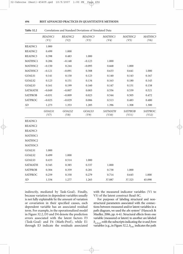
both completely mediated by Task-Goal. InModel 2 (Figure 32.1b), only the effect of Read-SC on Math-Prof is completely mediated byTask-Goal, while Math-SC affects Math-Profnot only indirectly via Task-Goal but alsodirectly without other intervening variables.Finally, in Model 3 (Figure 32.1c), Read-SC andMath-SC are thought to affect Math-Profdirectly as well as indirectly via Task-Goal. Toillustrate the testing of the tenability of thesethree competing models, multivariate normaldata on three indicator variables for each of thefour constructs were simulated for a sample ofn = 1,000 ninth-grade girls. Table 32.1 describesthe 12 indicator variables in more detail, whileTable 32.2 contains relevant summary statistics.1

At this point, it is possible and might seementirely appropriate to address the research ques-tions implied by the hypothesized models througha series of multiple linear regression (MLR) analy-ses. For example, for Model 2 in Figure 32.1b, twoseparate regressions could be conducted: (1) Anappropriate surrogate measure of Math-Profcould be regressed on proxy variables for Math-SC and Task-Goal, and (2) a suitable indicator ofTask-Goal could be regressed on proxies for Read-SC and Math-SC. If the researcher would chooseitems ReadSC3, MathSC3, TG1, and Proc fromTable 32.1 as surrogates for their respective con-structs, MLR results would indicate that eventhough all hypothesized effects are statistically sig-nificantly different from zero, only small amountsof variance in the dependent variables TG1 andProc are explained by their respective predictorvariables (R2

TG1 = 0.034, R2Proc = 0.26; see Table

32.6 for the unstandardized and standardizedregression coefficients obtained from the twoMLR analyses2). As we will show through thecourse of the illustrations below, an appropriatelyconducted LVPA of the models in Figure 32.1 andthe data in Table 32.2 will greatly enhance the util-ity of the data to extract more meaningful resultsthat address the researcher’s key questions.

SEM Notation

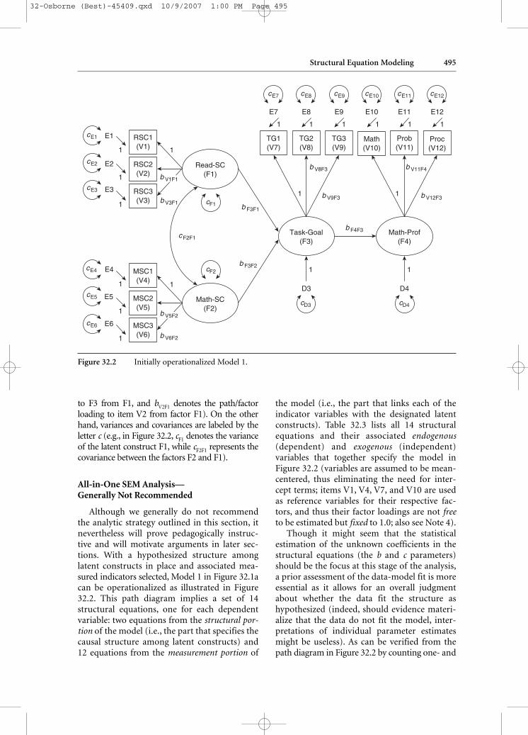
As the three alternative structural modelsdepicted in Figure 32.1 are at the theoretical/latent construct level, we followed commonpractice and enclosed the four factors of Read-SC, Math-SC, Task-Goal, and Math-Prof inellipses/circles. On the other hand, a glanceahead at the operationalized model in Figure 32.2reveals that the now included measured variables



Read-SC(F1)

(a) Model 1

Task-Goal(F3)

Math-Prof(F4)

Math-SC(F2)

cF1

cF2

cD3 cD4

bF3F1

bF4F3

bF3F2

cF2F1

D3 D4

Read-SC(F1)

Task-Goal(F3)

Math-Prof(F4)

Math-SC(F2)

cF1

cF2

cD3 cD4

bF3F1

bF4F3

bF4F2bF3F2

cF2F1

D3 D4

(b) Model 2

Read-SC(F1)

Task-Goal(F3)

Math-Prof(F4)

Math-SC(F2)

cF1

cF2

cD3 cD4

bF3F1

bF4F3

bF4F2

bF4F1

bF3F2

cF2F1

D3 D4

(c) Model 3

Figure 32.1 The theoretical models.


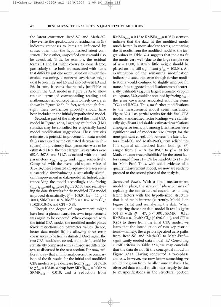
(items RSC1 to RSC3, MSC1 to MSC3, TG1 toTG3, Math, Prob, and Proc) are enclosed in rec-tangles/squares. Using the Bentler-Weeks“VFED” labeling convention (V for measuredVariable/item, F for latent Factor/construct, Efor Error/measured variable residual, D forDisturbance/latent factor residual), the latentand measured variables in the current modelsare labeled F1 through F4 and V1 through V12,respectively. The hypothesized presence orabsence of relations between variables in themodel is indicated by the presence or absence ofarrows in the corresponding path diagram:One-headed arrows signify direct structural orcausal effects hypothesized from one variable toanother, while two-headed arrows denote

hypothesized covariation and variation withoutstructural specificity. For example, for Model 1in Figure 32.1a, note (a) the hypothesizedcovariance between Read-SC and Math-SC andthe constructs’ depicted variances (two-headedarrows connect the factors to each other and tothemselves, given that a variable’s variance canbe thought of as a covariance of the variable with itself), (b) the hypothesized structuraleffects of these two factors on Task-Goal (one-headed arrows lead from both to Task-Goal),but (c) the absence of such hypothesized directeffects on Math-Prof (there are no one-headedarrows directly leading from Read-SC andMath-SC to Math-Prof; the former two con-structs are hypothesized to affect the latter only


Table 32.1 Indicator Variable/Item Description

Construct Variable Label Item Scores

Read-SC (F1)

RSC1 (V1) “Compared to others my age, 1 (false) to 6 (true)I am good at reading.”

RSC2 (V2) “I get good grades in reading.”

RSC3 (V3) “Work in reading class is easy for me.”

Math-SC (F2)

MSC1 (V4) “Compared to others my age, 1 (false) to 6 (true)I am good at math.”

MSC2 (V5) “I get good grades in math.”

MSC3 (V6) “Work in math class is easy for me.”

Task-Goal (F3)

TG1 (V7) “I like school work that I’ll learn 1 (false) to 6 (true)from, even if I make a lot of mistakes.”

TG2 (V8) “An important reason why I do my school work is because I like to learn new things.”

TG3 (V9) “I like school work best when it really makes me think.”

Math-Prof (F4)

Math (V10) Mathematics subtest scores of the Stanford Achievement Test 9

Prob (V11) Problem Solving subtest scores of the Stanford Achievement Test 9

Proc (V12) Procedure subtest scores of the Stanford Achievement Test 9



indirectly, mediated by Task-Goal). Finally,because variation in dependent variables usuallyis not fully explainable by the amount of variationor covariation in their specified causes, eachdependent variable has an associated residualterm. For example, in the operationalized modelin Figure 32.2, D3 and D4 denote the predictionerrors associated with the latent factors F3(Task-Goal) and F4 (Math-Prof), while E1through E3 indicate the residuals associated

with the measured indicator variables (V1 toV3) of the latent construct Read-SC.

For purposes of labeling structural and non-structural parameters associated with the connec-tions between measured and/or latent variables in apath diagram, we used the abc system3 (Hancock &Mueller, 2006, pp. 4–6). Structural effects from onevariable (measured or latent) to another are labeledbto, from, with the subscripts indicating the to and fromvariables (e.g., in Figure 32.2, bF3F1 indicates the path

Table 32.2 Correlations and Standard Deviations of Simulated Data

READSC1 READSC2 READSC3 MATHSC1 MATHSC2 MATHSC3(V1) (V2) (V3) (V4) (V5) (V6)

READSC1 1.000

READSC2 0.499 1.000

READSC3 0.398 0.483 1.000

MATHSC1 0.206 –0.148 –0.123 1.000

MATHSC2 –0.150 0.244 –0.095 0.668 1.000

MATHSC3 –0.121 –0.091 0.308 0.633 0.641 1.000

GOALS1 0.141 0.150 0.123 0.140 0.143 0.167

GOALS2 0.123 0.151 0.134 0.163 0.180 0.145

GOALS3 0.161 0.199 0.160 0.147 0.151 0.158

SATMATH –0.049 –0.007 0.003 0.556 0.539 0.521

SATPROB –0.031 –0.009 0.023 0.544 0.505 0.472

SATPROC –0.025 –0.029 0.006 0.513 0.483 0.480

SD 1.273 1.353 1.285 1.396 1.308 1.300

GOALS1 GOALS2 GOALS3 SATMATH SATPROB SATPROC (V7) (V8) (V9) (V10) (V11) (V12)

READSC1

READSC2

READSC3

MATHSC1

MATHSC2

MATHSC3

GOALS1 1.000

GOALS2 0.499 1.000

GOALS3 0.433 0.514 1.000

SATMATH 0.345 0.385 0.337 1.000

SATPROB 0.304 0.359 0.281 0.738 1.000

SATPROC 0.259 0.330 0.279 0.714 0.645 1.000

SD 1.334 1.277 1.265 37.087 37.325 45.098



to F3 from F1, and bV2F1 denotes the path/factorloading to item V2 from factor F1). On the otherhand, variances and covariances are labeled by theletter c (e.g., in Figure 32.2, cF1 denotes the varianceof the latent construct F1, while cF2F1 represents thecovariance between the factors F2 and F1).

All-in-One SEM Analysis—Generally Not Recommended

Although we generally do not recommendthe analytic strategy outlined in this section, itnevertheless will prove pedagogically instruc-tive and will motivate arguments in later sec-tions. With a hypothesized structure amonglatent constructs in place and associated mea-sured indicators selected, Model 1 in Figure 32.1acan be operationalized as illustrated in Figure32.2. This path diagram implies a set of 14structural equations, one for each dependentvariable: two equations from the structural por-tion of the model (i.e., the part that specifies thecausal structure among latent constructs) and12 equations from the measurement portion of

the model (i.e., the part that links each of theindicator variables with the designated latentconstructs). Table 32.3 lists all 14 structuralequations and their associated endogenous(dependent) and exogenous (independent) variables that together specify the model inFigure 32.2 (variables are assumed to be mean-centered, thus eliminating the need for inter-cept terms; items V1, V4, V7, and V10 are usedas reference variables for their respective fac-tors, and thus their factor loadings are not freeto be estimated but fixed to 1.0; also see Note 4).

Though it might seem that the statisticalestimation of the unknown coefficients in thestructural equations (the b and c parameters)should be the focus at this stage of the analysis,a prior assessment of the data-model fit is moreessential as it allows for an overall judgmentabout whether the data fit the structure ashypothesized (indeed, should evidence materi-alize that the data do not fit the model, inter-pretations of individual parameter estimatesmight be useless). As can be verified from thepath diagram in Figure 32.2 by counting one- and

cE7

cE1

cE2

cE3

cE4

cE5

cE6

cE8 cE9 cE10 cE11 cE12

cD3 cD4

b V3F1 cF1

cF2

Proc(V12)

Prob(V11)

Math(V10)

TG3(V9)

TG2(V8)

TG1(V7)

E7 E8 E9 E10 E11 E12

b V6F2

b V8F3

b V9F3 b V12F3

b F4F3

b F3F2

b F3F1

cF2F1

b V11F4

D3

E4

E1

E2

E3

E5

E6

D4

Math-Prof(F4)

Task-Goal(F3)

1

1

1

1

Math-SC(F2)

Read-SC(F1)

RSC3(V3)

RSC2(V2)

RSC1(V1)

MSC1(V4)

MSC2(V5)

MSC3(V6)

1 1 1 1 1 1

1

1

1

1

1

1

1 1

b V1F1

b V5F2

Figure 32.2 Initially operationalized Model 1.



Table 32.3 Structural Equations Implied by the Path Diagram in Figure 32.2

Structural Portion

Endogenous Variable Structural Equations Exogenous Variablesa

Task-Goal (F3) F3 = bF3F1 F1 + bF3F2 F2 + D3 Read-SC (F1)Math-SC (F2)

Math-Prof (F4) F4 = bF4F3 F3 + D4 Task-Goal (F3)

Measurement Portion

Endogenous Variable Structural Equations Exogenous Variablesb

RSC1 (V1) V1 = (1)F1 + E1 Read-SC (F1)

RSC2 (V2) V2 = bV2F1 F1 + E2

RSC3 (V3) V3 = bV3F1 F1 + E3

MSC1 (V4) V4 = (1)F2 + E4 Math-SC (F2)

MSC2 (V5) V5 = bV5F2 F2 + E5

MSC3 (V6) V6 = bV6F2 F2 + E6

TG1 (V7) V7 = (1)F3 + E7 Task-Goal (F3)

TG2 (V8) V8 = bV8F3 F3 + E8

TG3 (V9) V9 = bV9F3 F3 + E9

Math (V10) V10 = (1)F4 + E10 Math-Prof (F4)

Prob (V11) V11 = bV11F4 F4 + E11

Proc (V12) V12 = bV12F4 F4 + E12

a. Residuals D, though technically independent, are not listed.

b. Residuals E, though technically independent, are not listed.

two-headed arrows labeled with b or c symbols,the model contains t = 28 parameters to be esti-mated:4 two variances of the independent latentconstructs and one covariance between them,two variances of residuals associated with thetwo dependent latent constructs, three pathcoefficients relating the latent constructs, eightfactor loadings, and 12 variances of residualsassociated with the measured variables. Further-more, the 12 measured variables in the modelproduce u = 12 (12 + 1)/2 = 78 unique variancesand covariances; the model is overidentified (t =28 < u = 78), and it is likely that some degree ofdata-model misfit exists (i.e., the observedcovariance matrix will likely differ, to somedegree, from that implied by the model). Toassess the degree of data-model misfit, variousfit indices can be obtained and then should becompared against established cutoff criteria(e.g., those empirically derived by Hu & Bentler,1999, and listed here in Table 32.4). Thoughhere LISREL 8.8 (Jöreskog & Sörbom, 2006)

was employed, running any of the availableSEM software packages will verify the followingdata-model fit results for the data in Table 32.2and the model in Figure 32.2 (because the dataare assumed multivariate normal, the maxi-mum likelihood estimation method was used):χ2 = 3624.59 (df = u – t = 50, p < .001), SRMR =0.13, RMSEA = 0.20 with CI90: (0.19, 0.20), andCFI = 0.55.

As is evident from comparing these resultswith the desired values in Table 32.4, the currentdata do not fit the proposed model; thus, it isnot appropriate to interpret any individual para-meter estimates as, on the whole, the model inFigure 32.2 should be rejected based on the cur-rent data. Now the researcher is faced with thequestion of what went wrong: (a) Is the sourceof the data-model misfit indeed primarily a flawin the underlying structural theory (Figure 32.1a),(b) can the misfit be attributed to misspecifica-tions in the measurement portion of the modelwith the hypothesized structure among latent


constructs actually having been specified cor-rectly, or (c) do misspecifications exist in boththe measurement and structural portions of themodel? To help address these questions and pre-vent potential confusion about the source ofobserved data-model misfit, we do not recom-mend that researchers conduct SEM analyses byinitially analyzing the structural and measure-ment portions of their model simultaneously,as was done here. Instead, analysts are urged tofollow a two-phase analysis process, as describednext.

Two-Phase SEM Analysis—Recommended

Usually, the primary reason for conceptualiz-ing LVPA models is to investigate the tenabilityof theoretical causal structures among latentvariables. The main motivation for recommend-ing a two-phase process over an all-in-oneapproach is to initially separate a model into itsmeasurement and structural portions so thatmisspecifications in the former, if present, canbe realized and addressed first, before the struc-ture among latent constructs is assessed.5 Thisapproach will simplify the identification ofsources of data-model misfit and might also aidin the prevention of nonconvergence problemswith SEM software (i.e., when the iterative esti-mation algorithm cannot converge upon aviable solution for parameter estimates).

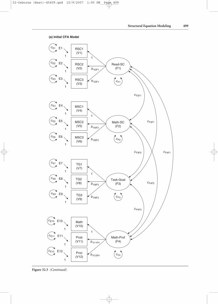
Consider the path diagram in Figure 32.3a. Itis similar to the one depicted in Figure 32.2 as itinvolves the same measured and latent variablesbut differs in two important ways: Not only areRead-SC and Math-SC now explicitly connectedto Math-Prof, but all structural links amonglatent variables have been changed to nonstruc-tural relations (note in Figure 32.3a the two-headed arrows between all latent constructs thatare now labeled with c symbols). That is, latentconstructs are allowed to freely covary withoutan explicit causal structure among them. Inshort, Figure 32.3a represents a CFA model ofthe latent factors Read-SC, Math-SC, Task-Goal,and Math-Prof, using the measured variables inTable 32.1 as their respective effect indicators.6

Measurement Phase. An analysis of the CFAmodel in Figure 32.3a constitutes the beginningof the measurement phase of the proposed two-phase analysis process and produced the follow-ing data-model fit results: χ2 = 3137.16 (df = 48,p < .001), SRMR = 0.062, RMSEA = 0.18 withCI90: (0.17, 0.18), and CFI = 0.61. These valuessignify a slight improvement over fit results forthe model in Figure 32.2. To the experiencedmodeler, this improvement was predictablegiven that the model in Figure 32.2 is morerestrictive than, and a special case of, the CFAmodel in Figure 32.3a (with the paths fromRead-SC and Math-SC to Math-Prof fixed tozero); that is, the former model is nested withinthe latter, a topic more fully discussed in the nextsection. Irrespective of this minor improvement,however, why did the data-model fit remainunsatisfactory (as judged by the criteria listed inTable 32.4)? Beginning to analyze and addressthis misfit constitutes a move toward the fourthand final phase in the general SEM process,potential post hoc model modification.

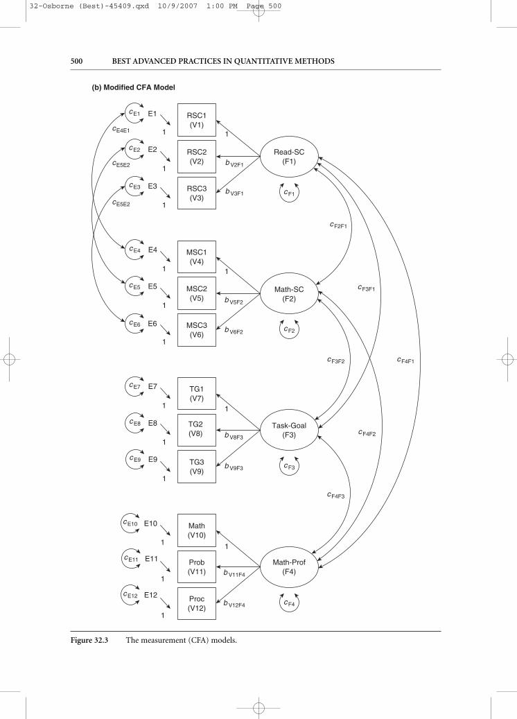
First, reconsider the list of items in Table 32.1.While all variables certainly seem to “belong” tothe latent factors they were selected to indicate,note that for the reading and mathematics self-concept factors, corresponding items are identicalexcept for one word: The word reading in itemsRSC1 through RSC3 was replaced by the wordmath to obtain items MSC1 through MSC3. Thus,it seems plausible that individuals’ responses tocorresponding reading and mathematics self-con-cept items are influenced by some of the same orrelated causes. In fact, the model in Figure 32.3aexplicitly posits that two such related causes are


Table 32.4 Target Values for Selected Fit Indicesto Retain a Model by Class

Index Class

Incremental Absolute Parsimonious

NFI ≥ 0.90

NNFI ≥ 0.95 GFI ≥ 0.90 AGFI ≥ 0.90

CFI ≥ 0.95 SRMR ≤ 0.08 RMSEA ≤ 0.06

Joint Criteria

NNFI, CFI ≥ 0.96 and SRMR ≤ 0.09

SRMR ≤ 0.09 and RMSEA ≤ 0.06

SOURCE: Partially taken from Hu and Bentler (1999).

NOTE: CFI = comparative fit index; NFI = normed fit index;NNFI = nonnormed fit index; GFI = goodness-of-fit index;AGFI = adjusted goodness-of-fit index; RMSEA = root meansquare error of approximation; SRMR = standardized rootmean square residual.



the latent constructs Read-SC and Math-SC.However, as the specification of residual terms (E)indicates, responses to items are influenced bycauses other than the hypothesized latent con-structs. Those other, unspecified causes could alsobe associated. Thus, for example, the residualterms E1 and E4 might covary to some degree,particularly since both are associated with itemsthat differ by just one word. Based on similar the-oretical reasoning, a nonzero covariance mightexist between E2 and E5 and also between E3 andE6. In sum, it seems theoretically justifiable tomodify the CFA model in Figure 32.3a to allowresidual terms of corresponding reading andmathematics self-concept items to freely covary, asshown in Figure 32.3b. In fact, with enough fore-sight, these covariances probably should havebeen included in the initially hypothesized model.

Second, as part of the analysis of the initial CFAmodel in Figure 32.3a, Lagrange multiplier (LM)statistics may be consulted for empirically basedmodel modification suggestions. These statisticsestimate the potential improvement in data-modelfit (as measured by the estimated decrease in chi-square) if a previously fixed parameter were to beestimated. Here, the three largest LM statistics were652.0, 567.8, and 541.7, associated with the fixedparameters cE5E2, cE4E1, and cE6E3, respectively.Compared with the overall chi-square value of3137.16, these estimated chi-square decreases seemsubstantial,7 foreshadowing a statistically signifi-cant improvement in data-model fit. Indeed, afterrespecifying the model accordingly (i.e., freeingcE5E2, cE4E1, and cE6E3; see Figure 32.3b) and reanalyz-ing the data, fit results for the modified CFA modelimproved dramatically: χ2 = 108.04 (df = 45, p <.001), SRMR = 0.018, RMSEA = 0.037 with CI90:(0.028, 0.046), and CFI = 0.99.

Though the degree of improvement mighthave been a pleasant surprise, some improvementwas again to be expected: When compared withthe initial CFA model, the modified model placesfewer restrictions on parameter values (hence,better data-model fit) by allowing three errorcovariances to be freely estimated. Once again, thetwo CFA models are nested, and their fit could bestatistically compared with a chi-square differencetest, as discussed in the next section. For now, suf-fice it to say that an informal, descriptive compar-ison of the fit results for the initial and modifiedCFA models (e.g., a decrease from χ2

initial = 3137.16to χ2

mod = 108.04, a drop from SRMRinitial = 0.062 toSRMRmod = 0.018, and a reduction from

RMSEAinitial = 0.18 to RMSEAmod = 0.037) seems toindicate that the data fit the modified modelmuch better. In more absolute terms, comparingthe fit results from the modified model to the tar-get values in Table 32.4 suggests that the data fitthe model very well (due to the large sample sizeof n = 1,000, relatively little weight should beplaced on the still significant χ2

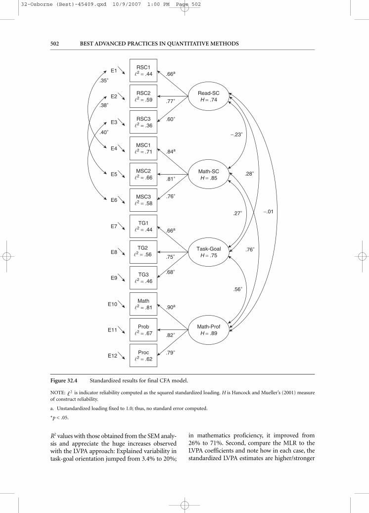
(45) = 108.04). Anexamination of the remaining modificationindices indicated that, even though further modi-fications would continue to slightly improve fit,none of the suggested modifications were theoret-ically justifiable (e.g., the largest estimated drop inchi-square, 23.0, could be obtained by freeing cE8E2,the error covariance associated with the itemsTG2 and RSC2). Thus, no further modificationsto the measurement model seem warranted.Figure 32.4 lists partial results for this final CFAmodel: Standardized factor loadings were statisti-cally significant and sizable, estimated correlationsamong error terms and among latent factors weresignificant and of moderate size (except for thenonsignificant correlation between the latent fac-tors Read-SC and Math-Prof), item reliabilities(the squared standardized factor loadings, )ranged from = .36 for RSC3 to = .81 forMath, and construct reliabilities8 for the latent fac-tors ranged from H = .74 for Read-SC to H = .89for Math-Prof. Thus, with solid evidence of aquality measurement model, we now are ready toproceed to the second phase of the analysis.

Structural Phase. With a final measurementmodel in place, the structural phase consists ofreplacing the nonstructural covariances amonglatent factors with the hypothesized structurethat is of main interest (currently, Model 1 inFigure 32.1a) and reanalyzing the data. Whencomparing these new data-model fit results (χ2 =601.85 with df = 47, p < .001, SRMR = 0.12,RMSEA = 0.10 with CI90: [0.096, 0.11], and CFI =0.93) to those from the final CFA model, welearn that the introduction of two key restric-tions—namely, the a priori specified zero pathsfrom Read-SC and Math-SC to Math-Prof—significantly eroded data-model fit.9 Consultingcutoff criteria in Table 32.4, we may concludethat the data do not fit the conceptual model inFigure 32.1a. Having conducted a two-phaseanalysis, however, we now know something wecould not glean from the all-in-one analysis: Theobserved data-model misfit must largely be dueto misspecifications in the structural portion

222



Read-SC(F1)

Math-SC(F2)

Task-Goal(F3)

Math-Prof(F4)

RSC1(V1)

RSC2(V2)

RSC3(V3)

MSC1(V4)

MSC2(V5)

MSC3(V6)

TG1(V7)

TG2(V8)

TG3(V9)

Math(V10)

Prob(V11)

Proc(V12)

b V11F4

cF4F3

cF4

cF2

cF3

cF1

cE1

cE2

cF4F2

cF3F2

cF3F1

cF2F1

cF4F1

b V8F3

b V6F2

b V5F2

b V2F1

b V3F1

b V9F3

b V12F4

E1

E2

cE3 E3

cE4 E4

cE5 E5

cE6 E6

cE7 E7

cE8 E8

cE9 E9

cE10 E10

cE11 E11

cE12 E12

1

1

1

1

1

1

1

1

1

1

1

11

(a) Initial CFA Model

1

1

1

Figure 32.3 (Continued)



Figure 32.3 The measurement (CFA) models.

Read-SC(F1)

Math-SC(F2)

Task-Goal(F3)

Math-Prof(F4)

RSC1(V1)

RSC2(V2)

RSC3(V3)

MSC1(V4)

MSC2(V5)

MSC3(V6)

TG1(V7)

TG2(V8)

TG3(V9)

Math(V10)

Prob(V11)

Proc(V12)

b V11F4

cF4F3

cF4

cF2

cF3

cF1

cE1

cE2

cF4F2

cF3F2

cF3F1

cF2F1

cF4F1

b V8F3

b V6F2

b V5F2

cE5E2

cE5E2

cE4E1

b V2F1

b V3F1

b V9F3

b V12F4

E1

E2

cE3 E3

cE4 E4

cE5 E5

cE6 E6

cE7 E7

cE8 E8

cE9 E9

cE10 E10

cE11 E11

cE12 E12

1

1

1

1

1

1

1

1

1

1

1

1 1

1

1

1

(b) Modified CFA Model



of the model since modifications to the mea-surement portion of the model (freeing errorcovariances for corresponding reading andmathematics self-concept items) led to a CFAmodel with no evidence of substantial data-model misfit. Having not yet reached a statewhere the data fit the hypothesized structure toan acceptable degree, we forego an interpretationof individual parameter estimates for a whilelonger in favor of illustrating how to compareand choose among the current model (Model 1)and the two remaining a priori hypothesizedstructures (Models 2 and 3) in Figure 32.1.

Choosing From Among Nested Models

Thus far in the illustrations, the comparison ofmodels with respect to data-model fit could beaccomplished only by descriptively weighing vari-ous fit index values across models. However, in thespecial case when two models, say Model 1 andModel 2, are nested (such as when the estimatedparameters in the former are a proper subset ofthose associated with the latter), fit comparisonscan be accomplished with a formal chi-square dif-ference test. That is, if Model 1 (with df1) is nestedwithin Model 2 (with df2), their chi-square fit sta-tistics may be statistically compared by ∆χ2

(df1– df

2) =

χ2(df

1) − χ2

(df2), which is distributed as a chi-square

distribution with df = df1 – df2 (under conditionsof multivariate normality).

Now reconsider the three theoretical modelsin Figure 32.1, all now incorporating the finalmeasurement model in Figure 32.3b. As the fitinformation in Table 32.5 shows, Models 2 and 3seem to fit well,10 while Model 1 does not, as pre-viously discussed. Furthermore, note that Model1, the most parsimonious and restrictive model,is nested within both Models 2 and 3 (lettingbF4F2 ≠ 0 in Model 1 leads to Model 2; allowingboth bF4F2 ≠ 0 and bF4F1 ≠ 0 in Model 1 leads toModel 3) and that Model 2 is nested in Model 3(permitting bF4F1 ≠ 0 in Model 2 leads to Model 3).Thus, the chi-square fit statistics for the threecompeting models can easily be compared bychi-square difference tests. Based on the threepossible chi-square comparisons shown in Table32.5, we glean that out of the three alternatives,Model 2 is the preferred structure (when weigh-ing chi-square fit and parsimony):

1. Both Models 2 and 3 are chosen over Model 1 (they both exhibit significantly

better fit, ∆ χ2(1) = 492.56, p < .001; ∆ χ2

(2) =493.81, p < .001; respectively), and

2. Model 2 is favored over Model 3 (even thoughit is more restrictive—but hence moreparsimonious—the erosion in fit isnonsignificant, ∆ χ2

(1) = 1.25, p = .264).

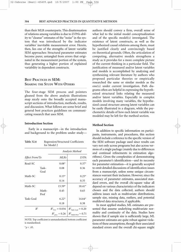
Having chosen Model 2 from among thethree alternative models and judging its data-model fit as acceptable (Table 32.5), whatremains is an examination and interpretation ofthe structural parameter estimates that link thelatent constructs (see Table 32.6; interpretationsof results from the measurement phase are listedin Figure 32.4 and were examined earlier). Notethat the latent factors Read-SC and Math-SCexplained 20% of the variance in Task-Goal (R2 =0.20) and that those three factors explained morethan 70% of the variance in latent mathematicsproficiency (R2 = 0.71). All structural estimateswere statistically significant and can be inter-preted in a manner similar to regression coeffi-cients, but now with a focus on structuraldirection, given the specific causal nature of theunderlying hypothesized theory. For example,considering the standardized path coefficients,11

one might expect from within the context ofModel 2 that a one standard deviation increase inninth-grade girls’ latent reading self-conceptcauses, on average, a bit more than a third (0.36)of a standard deviation increase in their latenttask-goal orientation; similarly, a one standarddeviation increase in girls’ task-goal orientationleads, on average, to a 0.38 standard deviationincrease in latent mathematics proficiency. Giventhe hypothesized structure, the effect of readingself-concept on mathematics proficiency is com-pletely mediated by Task-Goal, with an estimatedstandardized indirect effect of 0.36 × 0.38 = 0.14(p < .05, as indicated by SEM software).

Finally, recall from the beginning of this sec-tion the two separate multiple linear regressionanalyses for a somewhat crude initial attempt ataddressing coefficient estimation for the struc-ture in Model 2. In addition to LVPA results,Table 32.6 also lists R2 values and the unstandard-ized and standardized regression coefficientsassociated with the two implied structural equa-tions (using the proxy variables ReadSC3 forlatent reading self-concept, MathSC3 for latentmathematics self-concept, TG1 for latent task-goal orientation, and Proc for latent mathematicsproficiency). First, compare the two regression



R2 values with those obtained from the SEM analy-sis and appreciate the huge increases observedwith the LVPA approach: Explained variability intask-goal orientation jumped from 3.4% to 20%;

in mathematics proficiency, it improved from26% to 71%. Second, compare the MLR to theLVPA coefficients and note how in each case, thestandardized LVPA estimates are higher/stronger

Read-SCH = .74

Math-SCH = .85

Task-GoalH = .75

Math-ProfH = .89

RSC12 = .44

RSC22 = .59

RSC32 = .36

MSC12 = .71

MSC22 = .66

MSC32 = .58

TG12 = .44

TG22 = .56

TG32 = .46

Math2 = .81

Prob2 = .67

Proc2 = .62

.82∗

.56∗

.76∗

.27∗

.28∗

−.23∗

−.01

.79∗

E1

E2

E3

E4

E5

E6

E7

E8

E9

E10

E11

E12

.90a

.68∗

.75∗

.76∗

.81∗

.84a

.60∗

.77∗

.35∗

.38∗

.40∗

.66a

.66a

Figure 32.4 Standardized results for final CFA model.

NOTE: is indicator reliability computed as the squared standardized loading. H is Hancock and Mueller’s (2001) measureof construct reliability.

a. Unstandardized loading fixed to 1.0; thus, no standard error computed.

*p < .05.

2


503

Tabl

e 32

.5D

ata-

Mod

el F

it a

nd

Ch

i-Sq

uar

e D

iffe

ren

ce T

ests

for

Nes

ted

Mod

els

Mod

el 2

Mod

el 3

χ2 (df,

p)SR

MR

RM

SEA

C

FIχ2 (d

f,p)

SRM

RR

MSE

A

CFI

CI 90

CI 90

109.

29

0.01

70.

036

0.99

108.

04

0.01

80.

037

0.99

(46,

< 0

.001

)(0

.027

,0.0

45)

(45,

< 0

.001

)(0

.028

,0.0

46)

Mod

el 1

∆χ2 (1

)=

χ2 Μ1

− χ2 Μ

2=

601.

85 −

109

.29

= 49

2.56

∆χ2 (2

)=

χ2 Μ1

− χ2 Μ

3=

601.

85 −

108

.04

= 49

3.81

χ2 (df,

p)SR

MR

RM

SEA

C

FI(d

f= 1

,p <

.001

)(d

f= 2

,p <

.001

)

CI 90

601.

85

0.12

0.10

0.

93

(47,

< 0

.001

)(0

.096

,0.1

1)

Mod

el 2

∆χ2 (1

)=

χ2 Μ2

− χ2 Μ

3=

109.

29 −

108

.04

= 1.

25

(df=

1,p

= .2

64)

NO

TE

:CFI

= c

ompa

rati

ve f

it in

dex;

RM

SEA

= r

oot

mea

n s

quar

e er

ror

ofap

prox

imat

ion

;SR

MR

= s

tan

dard

ized

roo

t m

ean

squ

are

resi

dual

.



than their MLR counterparts. This disattenuationof relations among variables is due to LVPA’s abil-ity to “cleanse” estimates of the “noise” in the sys-tem that was introduced by the indicatorvariables’ inevitable measurement error. Herein,then, lies one of the strengths of latent variableSEM approaches: Structural parameter estimatesbecome purer, untangled from errors that origi-nated in the measurement portion of the system,thus generating a higher portion of explainedvariability in dependent constructs.

BEST PRACTICES IN SEM:SHARING THE STUDY WITH OTHERS

The four-stage SEM process and pointersgleaned from the above analysis illustrationsmap nicely onto the broadly accepted manu-script sections of introduction, methods, results,and discussion. What follows are some brief andgeneral best practices guidelines on communi-cating research that uses SEM.

Introduction Section

Early in a manuscript—in the introductionand background to the problem under study—

authors should convey a firm, overall sense ofwhat led to the initial model conceptualizationand of the specific model(s) investigated. Theexistence of latent constructs, as well as thehypothesized causal relations among them, mustbe justified clearly and convincingly based on theoretical grounds. Often, the articulation ofcompeting, alternative models strengthens astudy as it provides for a more complete pictureof the current thinking in a particular field. Thejustification of measured and/or latent variablesand models is accomplished by analyzing andsynthesizing relevant literature by authors whoproposed particular theories or empiricallyresearched the same or similar models as theone(s) under current investigation. Path dia-grams often are helpful in expressing the hypoth-esized structural links relating the measuredand/or latent variables. Especially in complexmodels involving many variables, the hypothe-sized causal structure among latent variables canbe easily illustrated in a diagram, while the psy-chometric details of how each latent variable wasmodeled may be left for the method section.

Method Section

In addition to specific information on partici-pants, instruments, and procedures, this sectionshould include a reference to the specific version ofthe SEM software package used since results canvary not only across programs but also across ver-sions of a single package (mainly due to differencesand continual refinements in estimation algo-rithms). Given the complexities of demonstratingeach parameter’s identification—and its necessityfor parameter estimation—it is generally acceptedto omit detailed discussions of identification issuesfrom a manuscript, unless some unique circum-stances warrant their inclusion. However, since theaccuracy of parameter estimates, associated stan-dard errors, and the overall chi-square value alldepend on various characteristics of the indicatorschosen and the data collected, authors shouldaddress issues such as multivariate distributions,sample size, missing data, outliers, and potentialmultilevel data structures, if applicable.

In most applied studies, ML estimates are pre-sented that assume underlying multivariate nor-mality and continuity of the data. Studies haveshown that if sample size is sufficiently large, MLparameter estimates are quite robust against viola-tions of these assumptions, though their associatedstandard errors and the overall chi-square might

Table 32.6 Regression/Structural Coefficientsfor Model 2

Analysis Method

Effect From/To MLRs LVPA

Read-SC 0.08* 0.37*

Task- 0.08 0.36Goal

Math-SC 0.15* 0.25*

0.14 0.35

Math-SC 15.59* 18.41*

Math- 0.45 0.65Prof

Task-Goal 6.22* 14.64*

0.18 0.38

R2 R2TG1 = 0.034 R2

Task-Goal = 0.20

R2proc = 0.26 R2

Math-Prof = 0.71

NOTE: Top coefficient is unstandardized; bottom coefficientis standardized.

*p < .05.



not be (e.g., West, Finch, & Curran, 1995). Somehave suggested, as a rough guideline, a 5:1 ratio ofsample size to number of parameters estimated inorder to trust ML parameter estimates (but associ-ated standard errors and the model chi-square sta-tistic might still be compromised; e.g., Bentler &Chou, 1987). We hesitate to endorse such a “one-size-fits-all” suggestion for three reasons. First, ifdata are not approximately normal, then alternatestrategies such as the Satorra-Bentler rescaled sta-tistics should be employed that have larger samplesize requirements. Second, even under normality,methodological studies have illustrated that formodels with highly reliable factors, quite satisfac-tory solutions can be obtained with relatively smallsamples, while models with less reliable factorsmight require larger samples (e.g., Gagné &Hancock, 2006; Marsh, Hau, Balla, & Grayson,1998). Third, such general sample size recommen-dations ignore issues of statistical power to evalu-ate models as a whole or to test parameters withinthose models (see, e.g., Hancock, 2006).

If the model posits latent constructs, the choiceof indicators usually is justified in an instrumen-tation subsection. First, for each construct mod-eled, the reader should be able to determine ifeffect or cause indicators were chosen: Only theformer operationalize the commonly modeledlatent factors; the latter determine latent compos-ites (see Note 6). In some SEM analyses, emergentconstructs are erroneously treated as latent,implying a mismatch between the modeled andthe actual nature of the construct, hence leadingto the potential for incorrect inferences regardingthe relations the construct might have with otherportions of the model. Second, each latent con-struct should be defined by a sufficient number ofpsychometrically sound indicators: “Two might befine, three is better, four is best, and anything moreis gravy” (Kenny, 1979, p. 143). Doing so can pre-vent various identification and estimation prob-lems as well as ensure satisfactory constructreliability (since latent constructs are theoreticallyperfectly reliable but are measured by imperfectindicators, numerical estimates of construct relia-bility are likely to be less than 1.0 but can bebrought to satisfactory levels with the inclusion ofquality indicator variables; see, e.g., Hancock & Mueller, 2001). Finally, the scale of the indica-tor variables should be accommodated by the estimation method, where variables clearly yield-ing ordinal data might warrant the use of estima-tion strategies other than ML (see Finney &DiStefano, 2006).

Results Section

How authors structure the results section obvi-ously is dictated by the particular model(s) andresearch questions under study. Notwithstanding,it is the researcher’s responsibility to provide accessto data in order to facilitate verification of theobtained results: If moment-level data were ana-lyzed, a covariance matrix (or correlation matrixwith standard deviations) should be presented in atable or appendix; if raw data were used, informa-tion on how to obtain access should be provided.

When analyzing LVPA models, results fromboth the measurement and structural phasesshould be presented. For overidentified models,judging the overall quality of a hypothesized modelusually is presented early in the results section.Given that available data-model fit indices can leadto inconsistent conclusions, researchers shouldconsider fit results from different classes so readerscan arrive at a more complete picture regarding amodel’s acceptability (Table 32.4). Also, a compari-son of fit across multiple, a priori specified alterna-tive models can assist in weighing the relativemerits of favoring one model over others. As illus-trated, when competing models are nested, a for-mal chi-square difference test is available to judge ifa more restrictive—but also more parsimonious—model can explain the observed data equally well,without a significant loss in data-model fit (alter-native models that are not nested have tradition-ally been compared only descriptively—relative evaluations of AIC values are recommended, withsmaller values indicating better fit—but recentmethodological developments suggest statisticalapproaches as well; see Levy & Hancock, 2007).

If post hoc model modifications are performedfollowing unacceptable data-model fit from eitherthe measurement or structural phase of the analy-sis, authors owe their audience a detailed account ofthe nature and reasons (both statistical and theoret-ical) for the respecification(s), including summaryresults from Lagrange multiplier tests and revisedfinal fit results. If data-model fit has been assessedand deemed satisfactory, with or without respecifi-cation, more detailed results are presented, usuallyin the form of individual unstandardized and stan-dardized parameter estimates for each structuralequation of interest, together with associated stan-dard errors and/or test statistics and coefficients ofdetermination (R2). When latent variables are partof a model, estimates of their construct reliabilityshould be presented, with values ideally fallingabove .70 or .80 (see Hancock & Mueller, 2001).


Discussion Section

In the final section of a manuscript, authorsshould provide a sense of what implications theresults from the SEM analysis have on the theoryor theories that gave rise to the initial model(s).Claims that a well-fitting model was “con-firmed” or that a particular theory was proven tobe “true,” especially after post hoc respecifica-tions, should be avoided. Such statements aregrossly misleading given that alternative, struc-turally different, yet mathematically equivalentmodels always exist that would produce identi-cal data-model fit results and thus would explainthe data equally well (see Hershberger, 2006). Atmost, a model with acceptable fit may be inter-preted as one tenable explanation for the asso-ciations observed in the data. From thisperspective, a SEM analysis should be evaluatedfrom a disconfirmatory, rather than a confirma-tory, perspective: Based on unacceptable data-model fit results, theories can be shown to befalse but not proven to be true by acceptabledata-model fit (see also Mueller, 1997).

If evidence of data-model misfit was presentedand a model was modified based on statisticalresults from Lagrange multiplier tests, readersmust be made aware of potential model overfit-ting and the capitalization on chance. Statisticallyrather than theoretically based respecificationsare purely exploratory and might say little aboutthe true model underlying the data. While somemodel modifications seem appropriate and theo-retically justifiable (usually, minor respecifica-tions of the measurement portion are more easilydefensible than those in the structural portion ofa model), they only address internal specificationerrors and should be cross-validated with datafrom new and independent samples.12

Finally, the interpretation of individual parameter estimates can involve explicit causallanguage, as long as this is done from within thecontext of the particular causal theory proposedand the possibility/probability of alternativeexplanations is raised unequivocally. Thoughsome might disagree, we think that explicit causalstatements are more honest than implicit onesand are more useful in articulating a study’s prac-tical implications; after all, is not causality theultimate aim of science (see Shaffer, 1992, p. x)?In the end, SEM is a powerful disconfirmatorytool at the researcher’s disposal for testing andinterpreting theoretically derived causal hypothe-ses from within an a priori specified causal system

of observed and/or latent variables. However, weurge authors to resist the apparently still popularbelief that the main goal of SEM is to achieve sat-isfactory data-model fit results; rather, it is to getone step closer to the “truth.” If it is true that aproposed model does not reflect reality, thenreaching a conclusion of misfit between data andmodel should be a desirable goal, not one to beavoided by careless respecifications until satisfac-tory levels of fit are achieved.

CONCLUSION

Throughout the sections of this chapter, we haveattempted to provide an overview of what webelieve should be considered best practices intypical SEM applications. As is probably true forthe other quantitative methods covered in thisvolume, a little SEM knowledge is sometimes adangerous thing, especially with user-friendlysoftware making the mechanics of SEM increas-ingly opaque to the applied user. Before embrac-ing SEM as a potential analysis tool andreporting SEM-based studies, investigatorsshould gain fundamental knowledge from any ofthe introductory textbooks referenced at thebeginning of this chapter. In an effort to aid inthe conduct and publication of appropriate, ifnot exemplary, SEM utilizations, we offeredsome best practices guidelines, except one, savingit for last. While SEM offers a general and flexiblemethodological framework, investigators shouldnot hesitate to consider other analytical tech-niques—many covered in the present volume—that potentially address research questions muchmore clearly and directly. As it was explained tothe second author several years ago,“Just becauseall your friends are doing this ‘structural equa-tion modeling’ thing doesn’t mean you have to. Ifall your friends jumped off a cliff. . . .” (MartaFoldi,13 personal communication, 1992).

NOTES

1. Several indicator variables are rating scalesthat could be argued to provide ordinal-level ratherthan interval-level data. Given the relatively highnumber of scale points, however, we analyzed thesedata as if they were interval (see Finney & DiStefano, 2006).

2. Using different proxy variables, or evencomposites of indicators, would still yield attenuated




results as none of the options filter the inherentmeasurement error.

3. Only b and c coefficients are used here; theletter a denotes intercept and mean terms in theanalysis of mean structures.

4. To help ensure identification and to provide ametric for each latent factor, reference variables werespecified (i.e., one factor loading for each latentconstruct was fixed to 1.0 as indicated in Figure 32.2).

5. Here it is assumed that measured variablesof “high quality” were chosen to serve as indicatorvariables of the latent constructs (i.e., measuredvariables with relatively high factor loadings).Somewhat paradoxically, the use of low-qualityindicators in the measurement portion of the modelcan erroneously lead to an inference of acceptabledata-model fit regarding the structural portion (seeHancock & Mueller, 2007).

6. Effect indicators are measured variables thatare specified to be the structural effects of the latentconstructs that are hypothesized to underlie them(e.g., Bollen & Lennox, 1991). The analysis of modelsinvolving cause indicators—items that contribute tocomposite scores to form emergent factors, or latentcomposites—is theoretically different but alsopossible, albeit more difficult (see Kline, 2006).

7. Typically, LM statistics are not additive; that is,the chi-square statistic is not expected to drop by 1761.5(= 652.0 + 567.8 + 541.7).When a fixed parameter isestimated in a subsequent reanalysis,LM statistics forthe remaining fixed parametersusually change. Hence,theoretically justifiable model modifications motivatedby LM results should usually occur one parameter at atime unless there is a clear theoretical reason for freeingmultiple parameters at once, as is the case here.

8. One way to assess construct reliability isthrough Hancock and Mueller’s (2001, p. 202)coefficient H. H is a function of item reliabilities, l2

i ,and is computed by the equation

where k is the number of measured variablesassociated with a given latent factor.

9. Such a statistical comparison is possible witha chi-square difference test since the current modelis nested within the final measurement model, asexplained next.

10. Perceptive readers will have noticed that fitresults for Model 3 equal those previously discussedfor the final measurement model. Indeed, this is nocoincidence but an illustration of two equivalentmodels, that is, models that differ in structure butexhibit identical data-model fit for any data set (seeHershberger, 2006).

11. For a given sample, only the interpretation ofstandardized coefficients is meaningful as the latent

factor metrics are arbitrary (different choices forreference variables could lead to different latentmetrics); unstandardized coefficients can be useful ineffect comparisons across multiple samples or studies.

12. If this is impractical or impossible, a cross-validation index could be computed (see Browne &Cudeck, 1993).

13. Mrs. Foldi is the second author’s mother;she has no formal training in SEM or in any otherstatistical technique.

REFERENCES

Arbuckle, J. L. (2007). AMOS (Version 7) [Computersoftware]. Chicago: SPSS.

Bentler, P. M. (2006). EQS (Version 6.1) [Computersoftware]. Encino, CA: Multivariate Software.

Bentler, P. M., & Chou, C.-P. (1987). Practical issuesin structural equation modeling. SociologicalMethods & Research, 16, 78–117.

Bollen, K. A. (1989). Structural equations with latentvariables. New York: John Wiley.

Bollen, K. A., & Lennox, R. (1991). Conventionalwisdom on measurement: A structural equationperspective. Psychological Bulletin, 110, 305–314.

Boomsma, A. (2000). Reporting analyses ofcovariance structures. Structural EquationModeling: A Multidisciplinary Journal, 7,461–483.

Browne, M. W. (1984). Asymptotically distribution-free methods for the analysis of covariancestructures. British Journal of Mathematical andStatistical Psychology, 37, 62–83.

Browne, M. W., & Cudeck, R. (1993). Alternativeways of assessing model fit. In K. A. Bollen & J. S. Long (Eds.), Testing structural equationmodels (pp. 136–162). Newbury Park, CA: Sage.

Byrne, B. M. (1998). Structural equation modelingwith LISREL, PRELIS, and SIMPLIS. Mahwah,NJ: Lawrence Erlbaum.

Byrne, B. M. (2001). Structural equation modelingwith AMOS. Mahwah, NJ: Lawrence Erlbaum.

Byrne, B. M. (2006). Structural equation modelingwith EQS: Basic concepts, applications, andprogramming. Mahwah, NJ: Lawrence Erlbaum.

Finney, S. J., & DiStefano, C. (2006). Nonnormal andcategorical data in structural equationmodeling. In G. R. Hancock & R. O. Mueller(Eds.), Structural equation modeling: A secondcourse (pp. 269–314). Greenwich, CT:Information Age Publishing.

Gagné, P. E., & Hancock, G. R. (2006). Measurementmodel quality, sample size, and solutionpropriety in confirmatory factor models.Multivariate Behavioral Research, 41, 65–83.

Hancock, G. R. (2006). Power analysis in covariancestructure modeling. In G. R. Hancock & R. O.

H = 1

/[1 +

(1

/k∑

i=1

2i

/(1 − 2

i

))],


Mueller (Eds.), Structural equation modeling: A second course (pp. 69–115). Greenwich, CT:Information Age Publishing.

Hancock, G. R., & Mueller, R. O. (2001). Rethinkingconstruct reliability within latent variablesystems. In R. Cudeck, S. du Toit, & D. Sörbom(Eds.), Structural equation modeling: Present andfuture—A Festschrift in honor of Karl Jöreskog(pp. 195–216). Lincolnwood, IL: ScientificSoftware International, Inc.

Hancock, G. R., & Mueller, R. O. (2004). Path analysis.In M. Lewis-Beck, A. Brymann, & T. F. Liao(Eds.), Sage encyclopedia of social science researchmethods (pp. 802–806). Thousand Oaks, CA: Sage.

Hancock, G. R., & Mueller, R. O. (Eds.). (2006).Structural equation modeling: A second course.Greenwich, CT: Information Age Publishing.

Hancock, G. R., & Mueller, R. O. (2007, April). Thereliability paradox in structural equationmodeling fit indices. Paper presented at theannual meeting of the American EducationalResearch Association, Chicago.

Hershberger, S. L. (2003). The growth of structuralequation modeling: 1994–2001. StructuralEquation Modeling: A Multidisciplinary Journal,10, 35–46.

Hershberger, S. L. (2006). The problem of equivalentstructural models. In G. R. Hancock & R. O.Mueller (Eds.), Structural equation modeling: A second course (pp. 13–41). Greenwich, CT:Information Age Publishing.

Hoyle, R. H., & Panter, A. T. (1995). Writing aboutstructural equation models. In R. H. Hoyle(Ed.), Structural equation modeling: Concepts,issues, and applications (pp. 158–176).Thousand Oaks, CA: Sage.

Hu, L., & Bentler, P. M. (1999). Cutoff criteria for fitindexes in covariance structure analysis:Conventional criteria versus new alternatives.Structural Equation Modeling: AMultidisciplinary Journal, 6, 1–55.

Jöreskog, K. G. (1966). Testing a simple structurehypothesis in factor analysis. Psychometrika,31, 165–178.

Jöreskog, K. G. (1967). Some contributions tomaximum likelihood factor analysis.Psychometrika, 32, 443–482.

Jöreskog, K. G., & Sörbom, D. (2006). LISREL(Version 8.80) [Computer software].Lincolnwood, IL: Scientific SoftwareInternational.

Kaplan, D. (2000). Structural equation modeling:Foundations and extensions. Thousand Oaks,CA: Sage.

Kenny, D. A. (1979). Correlation and causation.New York: John Wiley.

Kline, R. B. (2005). Principles and practice of structuralequation modeling (2nd ed.). New York: Guilford.

Kline, R. B. (2006). Formative measurement andfeedback loops. In G. R. Hancock & R. O.Mueller (Eds.), Structural equation modeling: A second course (pp. 43–68). Greenwich, CT:Information Age Publishing.

Levy, R., & Hancock, G. R. (2007). A framework of statistical tests for comparing mean andcovariance structure models. MultivariateBehavioral Research, 42, 33–66.

Loehlin, J. C. (2004). Latent variable models (4th ed.).Hillsdale, NJ: Lawrence Erlbaum.

Marsh, H. W., Hau, K.-T., Balla, J. R., & Grayson, D.(1998). Is more ever too much? The number ofindicators per factor in confirmatory factoranalysis. Multivariate Behavioral Research, 33,181–220.

McDonald, R. P., & Ho, M. R. (2002). Principles andpractice in reporting structural equationanalyses. Psychological Methods, 7, 64–82.

Mueller, R. O. (1996). Basic principles of structuralequation modeling: An introduction to LISRELand EQS. New York: Springer-Verlag.

Mueller, R. O. (1997). Structural equation modeling:Back to basics. Structural Equation Modeling: A Multidisciplinary Journal, 4, 353–369.

Mueller, R. O., & Hancock, G. R. (2001). Factoranalysis and latent structure, confirmatory. InN. J. Smelser & P. B. Baltes (Eds.), Internationalencyclopedia of the social & behavioral sciences(pp. 5239–5244). Oxford, UK: Elsevier.

Muthén, B. O., & Muthén, L. K. (2006). Mplus(Version 4.1) [Computer software]. LosAngeles: Author.

Satorra, A., & Bentler, P. M. (1994). Corrections totest statistics and standard errors in covariancestructure analysis. In A. von Eye & C. C. Clogg(Eds.), Latent variables analysis: Applications fordevelopmental research (pp. 285–305).Thousand Oaks, CA: Sage.

Schumacker, R. E., & Lomax, R. G. (2004). Abeginner’s guide to structural equation modeling(2nd ed.). Mahwah, NJ: Lawrence Erlbaum.

Shaffer, J. P. (Ed.). (1992). The role of models innonexperimental social science: Two debates.Washington, DC: American EducationalResearch Association.

Tanaka, J. S. (1993). Multifaceted conceptions offit in structural equation models. In K. A.Bollen & J. S. Long (Eds.), Testing structuralequation models (pp. 10–39). Newbury Park,CA: Sage.

West, S. G., Finch, J. F., & Curran, P. J. (1995).Structural equation models with nonnormalvariables. In R. H. Hoyle (Ed.), Structural equationmodeling: Concepts, issues, and applications(pp. 56–75). Thousand Oaks, CA: Sage.

Wright, S. (1918). On the nature of size factors.Genetics, 3, 367–374.



509

33INTRODUCTION TO

BAYESIAN MODELING

FOR THE SOCIAL SCIENCES

GIANLUCA BAIO

MARTA BLANGIARDO

In the context of statistical problems, thefrequentist (or empirical) interpretation of probability has historically played a pre-

dominant role in modern statistics. In thisapproach, probability is defined as the limitingfrequency of occurrence in an infinitely repeatedexperiment. The underlying assumption is thatof a “fixed” concept of probability, which isunknown but can be theoretically disclosed bymeans of repeated trials, under the same exper-imental conditions.

However, although the frequentist approachstill plays the role of the standard in variousapplied areas, many other possible conceptual-izations of probability characterize differentphilosophies behind the problem of statisticalinference. Among these, an increasingly popularone is the Bayesian (also referred to as subjec-tivist), originated by the posthumous work ofReverend Thomas Bayes (1763)—see Howie(2002), Senn (2003), or Fienberg (2006) for ahistorical account of Bayesian theory.

The main feature of this approach is thatprobability is interpreted as a subjective degree

of belief in the occurrence of an event, repre-senting the individual level of uncertainty in itsactual realization (cf. de Finetti, 1974, probablythe most comprehensive account of subjectiveprobability). One of the main implications ofsubjectivism is that there is no requirement thatone should be able to specify, or even conceiveof, some relevant sequence of repetitions of theevent in question, as happens in the frequentistframework, with the advantage that events ofthe “one-off” type can be assessed consistently.

In the Bayesian philosophy, the probabilityassigned to any event depends also on the individ-ual whose uncertainty is being taken into accountand on the state of background informationunderlying this assessment. Varying any of thesefactors might change the probability. Consequently,under the subjectivist view, there is no assumptionof a unique, correct (or “true”) value for the prob-ability of any uncertain event (Dawid, 2005).Rather, each individual is entitled to his or her ownsubjective probability, and according to the evi-dence that becomes sequentially available, individ-uals tend to update their beliefs.1


Bayesian methods are not new to the socialsciences—from Phillips (1973) to Iversen(1984), Efron (1986), Raftery (1995), Berger(2000), and Gill (2002)—but they are also notsystematically integrated into most research inthe social sciences. This may be due to the com-mon perception among practitioners thatBayesian methods are “more complex.”

In fact, in our opinion, the apparent higherdegree of complexity is more than compensated byat least the two following consequences. First,Bayesian methods allow taking into account,through a formal model, all the available informa-tion, such as the results of previous studies.Moreover, the inferential process is straightfor-ward, as it is possible to make probabilistic state-ments directly on the quantities of interest (i.e.,some unobservable feature of the process understudy, typically represented by a set of parameters).

Despite their subjectivist nature, Bayesianmethods allow the practitioner to make the mostof the evidence: In just the situation of “repeatedtrials,” after observing the outcomes (successes andfailures) of many past trials (assuming no othersource of information), the individuals will bedrawn to an assessment of the probability of suc-cess on the next event that is extremely close to theobserved proportion of successes so far. However,if past data are not sufficiently extensive, it may be reasonably argued that there should indeed bescope for interpersonal disagreement as to theimplications of the evidence. Therefore, theBayesian approach provides a more general frame-work for the problem of statistical inference.2

In order to facilitate comprehension, we shallpresent two worked examples and switchbetween theory and practice in every section. Inthe first part of the chapter, we consider dataabout nonattendance at school for a set ofAustralian children, with additional informationabout their race (Aboriginal, White) and ageband also included. We use this data set to pre-sent the main feature of Bayesian reasoning andto follow the development of the simplest formof models (conjugated analysis). In the last sec-tion of the chapter, we describe a more realisticrepresentation for the analysis of SAT score data.The main objective of this analysis is to developa more complex model combining informationfor a number of related variables, using the sim-ulation techniques of Markov chain Monte Carlomethods.

CONDITIONAL PROBABILITIES

AND BAYES THEOREM

A fundamental concept in statistics, particularlywithin the Bayesian approach, is that of condi-tional probability (for a technical review, seeDawid, 1979). Given two events A and B, we candefine the event A | B (read “A given B”) as theoccurrence of the event A under the circumstancethat the event B has already occurred.

In other words, by considering the condi-tional probability, we are in fact changing the reference population; the probability of theevent A, Pr(A), is generally defined over thespace Ω, which contains all the possible eventsunder study, including A. Conversely, when con-sidering the conditional probability Pr(A | B), weare restricting our attention to the subspace of Ωwhere both the events A and B can occur. Such asubspace is indicated as (A & B). Moreover, thebasis of our comparison will not be Ω but just itssubspace where B is possible. Consequently, theprobability of the occurrence of the event A con-ditional on the event B is formally defined as

(1)

Example: Nonattendance at School in Australia

Paul and Banerjee (1998) studied Australianeducational data on the days of nonattendanceat school for 146 children by race (Aboriginal,White) and age band (primary, first form, sec-ond form, third form). The observed averagevalue of nonattendance days is 16, which will beused as a cutoff threshold for our analysis.

Suppose we are interested in the probabilitythat a student accumulates more than the aver-age number of nonattendance days, conditionalon his or her race. We can define the events ofinterest as follows:

H = >16 nonattendance days

W = White race

(where H stands for high nonattendance) andtheir complement as

Pr(A | B) = Pr(A&B)

Pr(B).



Documents

BEST PRACTICES IN STRUCTURAL EQUATION …...488 32 BEST PRACTICES IN STRUCTURAL EQUATION MODELING RALPH O. MUELLER GREGORY R. HANCOCK S tructural equation modeling (SEM) has evolved