Embed Size (px)
Citation preview

8/6/2019 Best Et Al._small-Scale Wind Energy Technical Report_2008
http://slidepdf.com/reader/full/best-et-alsmall-scale-wind-energy-technical-report2008 1/191

8/6/2019 Best Et Al._small-Scale Wind Energy Technical Report_2008
http://slidepdf.com/reader/full/best-et-alsmall-scale-wind-energy-technical-report2008 2/191

8/6/2019 Best Et Al._small-Scale Wind Energy Technical Report_2008
http://slidepdf.com/reader/full/best-et-alsmall-scale-wind-energy-technical-report2008 3/191
8/6/2019 Best Et Al._small-Scale Wind Energy Technical Report_2008
http://slidepdf.com/reader/full/best-et-alsmall-scale-wind-energy-technical-report2008 4/191

8/6/2019 Best Et Al._small-Scale Wind Energy Technical Report_2008
http://slidepdf.com/reader/full/best-et-alsmall-scale-wind-energy-technical-report2008 5/191

8/6/2019 Best Et Al._small-Scale Wind Energy Technical Report_2008
http://slidepdf.com/reader/full/best-et-alsmall-scale-wind-energy-technical-report2008 6/191

8/6/2019 Best Et Al._small-Scale Wind Energy Technical Report_2008
http://slidepdf.com/reader/full/best-et-alsmall-scale-wind-energy-technical-report2008 7/191

8/6/2019 Best Et Al._small-Scale Wind Energy Technical Report_2008
http://slidepdf.com/reader/full/best-et-alsmall-scale-wind-energy-technical-report2008 8/191

8/6/2019 Best Et Al._small-Scale Wind Energy Technical Report_2008
http://slidepdf.com/reader/full/best-et-alsmall-scale-wind-energy-technical-report2008 9/191

8/6/2019 Best Et Al._small-Scale Wind Energy Technical Report_2008
http://slidepdf.com/reader/full/best-et-alsmall-scale-wind-energy-technical-report2008 10/191
8/6/2019 Best Et Al._small-Scale Wind Energy Technical Report_2008
http://slidepdf.com/reader/full/best-et-alsmall-scale-wind-energy-technical-report2008 11/191

8/6/2019 Best Et Al._small-Scale Wind Energy Technical Report_2008
http://slidepdf.com/reader/full/best-et-alsmall-scale-wind-energy-technical-report2008 12/191

8/6/2019 Best Et Al._small-Scale Wind Energy Technical Report_2008
http://slidepdf.com/reader/full/best-et-alsmall-scale-wind-energy-technical-report2008 13/191

8/6/2019 Best Et Al._small-Scale Wind Energy Technical Report_2008
http://slidepdf.com/reader/full/best-et-alsmall-scale-wind-energy-technical-report2008 14/191

8/6/2019 Best Et Al._small-Scale Wind Energy Technical Report_2008
http://slidepdf.com/reader/full/best-et-alsmall-scale-wind-energy-technical-report2008 15/191
8/6/2019 Best Et Al._small-Scale Wind Energy Technical Report_2008
http://slidepdf.com/reader/full/best-et-alsmall-scale-wind-energy-technical-report2008 16/191

8/6/2019 Best Et Al._small-Scale Wind Energy Technical Report_2008
http://slidepdf.com/reader/full/best-et-alsmall-scale-wind-energy-technical-report2008 17/191

8/6/2019 Best Et Al._small-Scale Wind Energy Technical Report_2008
http://slidepdf.com/reader/full/best-et-alsmall-scale-wind-energy-technical-report2008 18/191
8/6/2019 Best Et Al._small-Scale Wind Energy Technical Report_2008
http://slidepdf.com/reader/full/best-et-alsmall-scale-wind-energy-technical-report2008 19/191

8/6/2019 Best Et Al._small-Scale Wind Energy Technical Report_2008
http://slidepdf.com/reader/full/best-et-alsmall-scale-wind-energy-technical-report2008 20/191

8/6/2019 Best Et Al._small-Scale Wind Energy Technical Report_2008
http://slidepdf.com/reader/full/best-et-alsmall-scale-wind-energy-technical-report2008 21/191

8/6/2019 Best Et Al._small-Scale Wind Energy Technical Report_2008
http://slidepdf.com/reader/full/best-et-alsmall-scale-wind-energy-technical-report2008 22/191

8/6/2019 Best Et Al._small-Scale Wind Energy Technical Report_2008
http://slidepdf.com/reader/full/best-et-alsmall-scale-wind-energy-technical-report2008 23/191

8/6/2019 Best Et Al._small-Scale Wind Energy Technical Report_2008
http://slidepdf.com/reader/full/best-et-alsmall-scale-wind-energy-technical-report2008 24/191
8/6/2019 Best Et Al._small-Scale Wind Energy Technical Report_2008
http://slidepdf.com/reader/full/best-et-alsmall-scale-wind-energy-technical-report2008 25/191

8/6/2019 Best Et Al._small-Scale Wind Energy Technical Report_2008
http://slidepdf.com/reader/full/best-et-alsmall-scale-wind-energy-technical-report2008 26/191
8/6/2019 Best Et Al._small-Scale Wind Energy Technical Report_2008
http://slidepdf.com/reader/full/best-et-alsmall-scale-wind-energy-technical-report2008 27/191
8/6/2019 Best Et Al._small-Scale Wind Energy Technical Report_2008
http://slidepdf.com/reader/full/best-et-alsmall-scale-wind-energy-technical-report2008 28/191

8/6/2019 Best Et Al._small-Scale Wind Energy Technical Report_2008
http://slidepdf.com/reader/full/best-et-alsmall-scale-wind-energy-technical-report2008 29/191

8/6/2019 Best Et Al._small-Scale Wind Energy Technical Report_2008
http://slidepdf.com/reader/full/best-et-alsmall-scale-wind-energy-technical-report2008 30/191

8/6/2019 Best Et Al._small-Scale Wind Energy Technical Report_2008
http://slidepdf.com/reader/full/best-et-alsmall-scale-wind-energy-technical-report2008 31/191

8/6/2019 Best Et Al._small-Scale Wind Energy Technical Report_2008
http://slidepdf.com/reader/full/best-et-alsmall-scale-wind-energy-technical-report2008 32/191

8/6/2019 Best Et Al._small-Scale Wind Energy Technical Report_2008
http://slidepdf.com/reader/full/best-et-alsmall-scale-wind-energy-technical-report2008 33/191

8/6/2019 Best Et Al._small-Scale Wind Energy Technical Report_2008
http://slidepdf.com/reader/full/best-et-alsmall-scale-wind-energy-technical-report2008 34/191
8/6/2019 Best Et Al._small-Scale Wind Energy Technical Report_2008
http://slidepdf.com/reader/full/best-et-alsmall-scale-wind-energy-technical-report2008 35/191

8/6/2019 Best Et Al._small-Scale Wind Energy Technical Report_2008
http://slidepdf.com/reader/full/best-et-alsmall-scale-wind-energy-technical-report2008 36/191

8/6/2019 Best Et Al._small-Scale Wind Energy Technical Report_2008
http://slidepdf.com/reader/full/best-et-alsmall-scale-wind-energy-technical-report2008 37/191

8/6/2019 Best Et Al._small-Scale Wind Energy Technical Report_2008
http://slidepdf.com/reader/full/best-et-alsmall-scale-wind-energy-technical-report2008 38/191

8/6/2019 Best Et Al._small-Scale Wind Energy Technical Report_2008
http://slidepdf.com/reader/full/best-et-alsmall-scale-wind-energy-technical-report2008 39/191

8/6/2019 Best Et Al._small-Scale Wind Energy Technical Report_2008
http://slidepdf.com/reader/full/best-et-alsmall-scale-wind-energy-technical-report2008 40/191

8/6/2019 Best Et Al._small-Scale Wind Energy Technical Report_2008
http://slidepdf.com/reader/full/best-et-alsmall-scale-wind-energy-technical-report2008 41/191

8/6/2019 Best Et Al._small-Scale Wind Energy Technical Report_2008
http://slidepdf.com/reader/full/best-et-alsmall-scale-wind-energy-technical-report2008 42/191

8/6/2019 Best Et Al._small-Scale Wind Energy Technical Report_2008
http://slidepdf.com/reader/full/best-et-alsmall-scale-wind-energy-technical-report2008 43/191

8/6/2019 Best Et Al._small-Scale Wind Energy Technical Report_2008
http://slidepdf.com/reader/full/best-et-alsmall-scale-wind-energy-technical-report2008 44/191

8/6/2019 Best Et Al._small-Scale Wind Energy Technical Report_2008
http://slidepdf.com/reader/full/best-et-alsmall-scale-wind-energy-technical-report2008 45/191

8/6/2019 Best Et Al._small-Scale Wind Energy Technical Report_2008
http://slidepdf.com/reader/full/best-et-alsmall-scale-wind-energy-technical-report2008 46/191

8/6/2019 Best Et Al._small-Scale Wind Energy Technical Report_2008
http://slidepdf.com/reader/full/best-et-alsmall-scale-wind-energy-technical-report2008 47/191

8/6/2019 Best Et Al._small-Scale Wind Energy Technical Report_2008
http://slidepdf.com/reader/full/best-et-alsmall-scale-wind-energy-technical-report2008 48/191

8/6/2019 Best Et Al._small-Scale Wind Energy Technical Report_2008
http://slidepdf.com/reader/full/best-et-alsmall-scale-wind-energy-technical-report2008 49/191

8/6/2019 Best Et Al._small-Scale Wind Energy Technical Report_2008
http://slidepdf.com/reader/full/best-et-alsmall-scale-wind-energy-technical-report2008 50/191

8/6/2019 Best Et Al._small-Scale Wind Energy Technical Report_2008
http://slidepdf.com/reader/full/best-et-alsmall-scale-wind-energy-technical-report2008 51/191

8/6/2019 Best Et Al._small-Scale Wind Energy Technical Report_2008
http://slidepdf.com/reader/full/best-et-alsmall-scale-wind-energy-technical-report2008 52/191

8/6/2019 Best Et Al._small-Scale Wind Energy Technical Report_2008
http://slidepdf.com/reader/full/best-et-alsmall-scale-wind-energy-technical-report2008 53/191

8/6/2019 Best Et Al._small-Scale Wind Energy Technical Report_2008
http://slidepdf.com/reader/full/best-et-alsmall-scale-wind-energy-technical-report2008 54/191

8/6/2019 Best Et Al._small-Scale Wind Energy Technical Report_2008
http://slidepdf.com/reader/full/best-et-alsmall-scale-wind-energy-technical-report2008 55/191
8/6/2019 Best Et Al._small-Scale Wind Energy Technical Report_2008
http://slidepdf.com/reader/full/best-et-alsmall-scale-wind-energy-technical-report2008 56/191

8/6/2019 Best Et Al._small-Scale Wind Energy Technical Report_2008
http://slidepdf.com/reader/full/best-et-alsmall-scale-wind-energy-technical-report2008 57/191

8/6/2019 Best Et Al._small-Scale Wind Energy Technical Report_2008
http://slidepdf.com/reader/full/best-et-alsmall-scale-wind-energy-technical-report2008 58/191

8/6/2019 Best Et Al._small-Scale Wind Energy Technical Report_2008
http://slidepdf.com/reader/full/best-et-alsmall-scale-wind-energy-technical-report2008 59/191
8/6/2019 Best Et Al._small-Scale Wind Energy Technical Report_2008
http://slidepdf.com/reader/full/best-et-alsmall-scale-wind-energy-technical-report2008 60/191

8/6/2019 Best Et Al._small-Scale Wind Energy Technical Report_2008
http://slidepdf.com/reader/full/best-et-alsmall-scale-wind-energy-technical-report2008 61/191

8/6/2019 Best Et Al._small-Scale Wind Energy Technical Report_2008
http://slidepdf.com/reader/full/best-et-alsmall-scale-wind-energy-technical-report2008 62/191
8/6/2019 Best Et Al._small-Scale Wind Energy Technical Report_2008
http://slidepdf.com/reader/full/best-et-alsmall-scale-wind-energy-technical-report2008 63/191

8/6/2019 Best Et Al._small-Scale Wind Energy Technical Report_2008
http://slidepdf.com/reader/full/best-et-alsmall-scale-wind-energy-technical-report2008 64/191
8/6/2019 Best Et Al._small-Scale Wind Energy Technical Report_2008
http://slidepdf.com/reader/full/best-et-alsmall-scale-wind-energy-technical-report2008 65/191
8/6/2019 Best Et Al._small-Scale Wind Energy Technical Report_2008
http://slidepdf.com/reader/full/best-et-alsmall-scale-wind-energy-technical-report2008 66/191

8/6/2019 Best Et Al._small-Scale Wind Energy Technical Report_2008
http://slidepdf.com/reader/full/best-et-alsmall-scale-wind-energy-technical-report2008 67/191
8/6/2019 Best Et Al._small-Scale Wind Energy Technical Report_2008
http://slidepdf.com/reader/full/best-et-alsmall-scale-wind-energy-technical-report2008 68/191

8/6/2019 Best Et Al._small-Scale Wind Energy Technical Report_2008
http://slidepdf.com/reader/full/best-et-alsmall-scale-wind-energy-technical-report2008 69/191
8/6/2019 Best Et Al._small-Scale Wind Energy Technical Report_2008
http://slidepdf.com/reader/full/best-et-alsmall-scale-wind-energy-technical-report2008 70/191

8/6/2019 Best Et Al._small-Scale Wind Energy Technical Report_2008
http://slidepdf.com/reader/full/best-et-alsmall-scale-wind-energy-technical-report2008 71/191

8/6/2019 Best Et Al._small-Scale Wind Energy Technical Report_2008
http://slidepdf.com/reader/full/best-et-alsmall-scale-wind-energy-technical-report2008 72/191

8/6/2019 Best Et Al._small-Scale Wind Energy Technical Report_2008
http://slidepdf.com/reader/full/best-et-alsmall-scale-wind-energy-technical-report2008 73/191

8/6/2019 Best Et Al._small-Scale Wind Energy Technical Report_2008
http://slidepdf.com/reader/full/best-et-alsmall-scale-wind-energy-technical-report2008 74/191

8/6/2019 Best Et Al._small-Scale Wind Energy Technical Report_2008
http://slidepdf.com/reader/full/best-et-alsmall-scale-wind-energy-technical-report2008 75/191

8/6/2019 Best Et Al._small-Scale Wind Energy Technical Report_2008
http://slidepdf.com/reader/full/best-et-alsmall-scale-wind-energy-technical-report2008 76/191

8/6/2019 Best Et Al._small-Scale Wind Energy Technical Report_2008
http://slidepdf.com/reader/full/best-et-alsmall-scale-wind-energy-technical-report2008 77/191

8/6/2019 Best Et Al._small-Scale Wind Energy Technical Report_2008
http://slidepdf.com/reader/full/best-et-alsmall-scale-wind-energy-technical-report2008 78/191

8/6/2019 Best Et Al._small-Scale Wind Energy Technical Report_2008
http://slidepdf.com/reader/full/best-et-alsmall-scale-wind-energy-technical-report2008 79/191

8/6/2019 Best Et Al._small-Scale Wind Energy Technical Report_2008
http://slidepdf.com/reader/full/best-et-alsmall-scale-wind-energy-technical-report2008 80/191

8/6/2019 Best Et Al._small-Scale Wind Energy Technical Report_2008
http://slidepdf.com/reader/full/best-et-alsmall-scale-wind-energy-technical-report2008 81/191

8/6/2019 Best Et Al._small-Scale Wind Energy Technical Report_2008
http://slidepdf.com/reader/full/best-et-alsmall-scale-wind-energy-technical-report2008 82/191

8/6/2019 Best Et Al._small-Scale Wind Energy Technical Report_2008
http://slidepdf.com/reader/full/best-et-alsmall-scale-wind-energy-technical-report2008 83/191

8/6/2019 Best Et Al._small-Scale Wind Energy Technical Report_2008
http://slidepdf.com/reader/full/best-et-alsmall-scale-wind-energy-technical-report2008 84/191

8/6/2019 Best Et Al._small-Scale Wind Energy Technical Report_2008
http://slidepdf.com/reader/full/best-et-alsmall-scale-wind-energy-technical-report2008 85/191
8/6/2019 Best Et Al._small-Scale Wind Energy Technical Report_2008
http://slidepdf.com/reader/full/best-et-alsmall-scale-wind-energy-technical-report2008 86/191
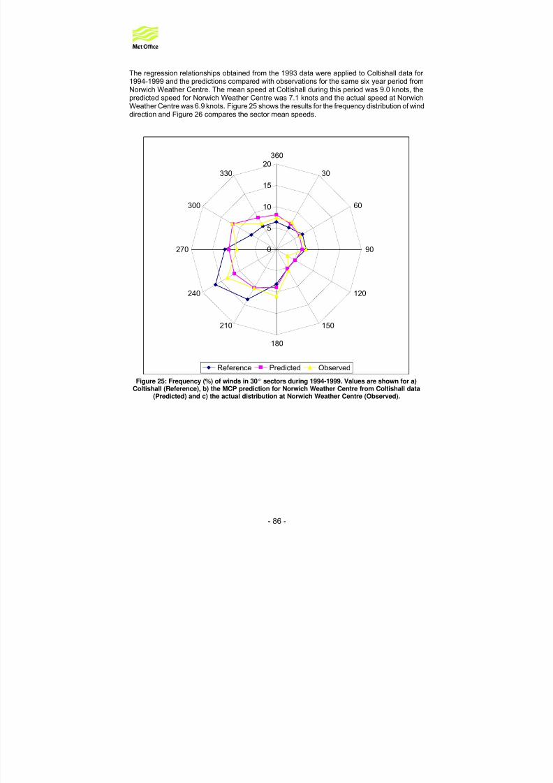
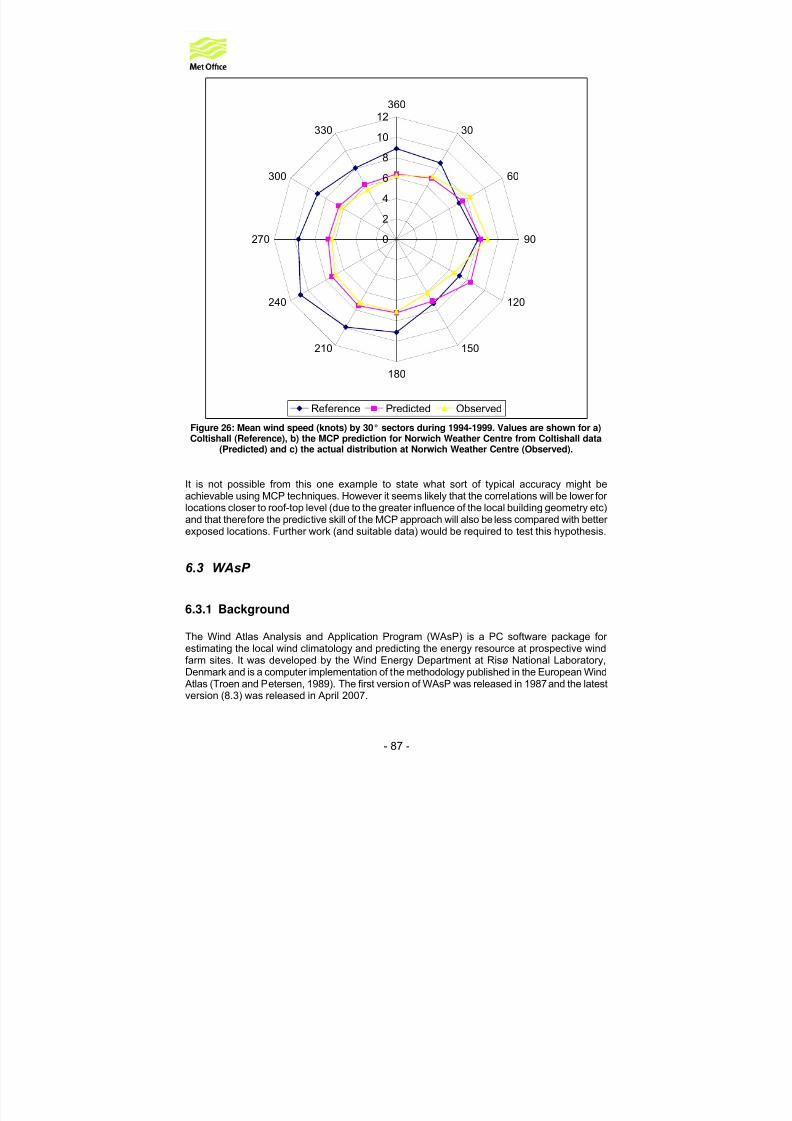
8/6/2019 Best Et Al._small-Scale Wind Energy Technical Report_2008
http://slidepdf.com/reader/full/best-et-alsmall-scale-wind-energy-technical-report2008 87/191
8/6/2019 Best Et Al._small-Scale Wind Energy Technical Report_2008
http://slidepdf.com/reader/full/best-et-alsmall-scale-wind-energy-technical-report2008 88/191

8/6/2019 Best Et Al._small-Scale Wind Energy Technical Report_2008
http://slidepdf.com/reader/full/best-et-alsmall-scale-wind-energy-technical-report2008 89/191

8/6/2019 Best Et Al._small-Scale Wind Energy Technical Report_2008
http://slidepdf.com/reader/full/best-et-alsmall-scale-wind-energy-technical-report2008 90/191

8/6/2019 Best Et Al._small-Scale Wind Energy Technical Report_2008
http://slidepdf.com/reader/full/best-et-alsmall-scale-wind-energy-technical-report2008 91/191

8/6/2019 Best Et Al._small-Scale Wind Energy Technical Report_2008
http://slidepdf.com/reader/full/best-et-alsmall-scale-wind-energy-technical-report2008 92/191

8/6/2019 Best Et Al._small-Scale Wind Energy Technical Report_2008
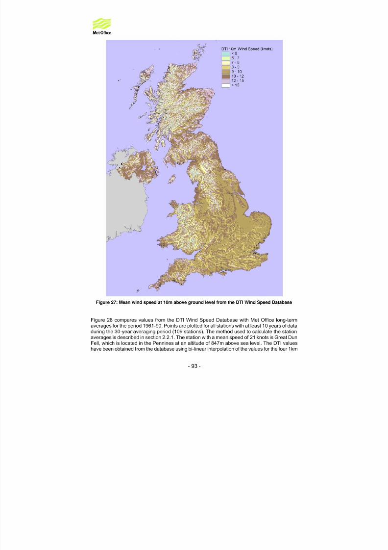
http://slidepdf.com/reader/full/best-et-alsmall-scale-wind-energy-technical-report2008 93/191
8/6/2019 Best Et Al._small-Scale Wind Energy Technical Report_2008
http://slidepdf.com/reader/full/best-et-alsmall-scale-wind-energy-technical-report2008 94/191
8/6/2019 Best Et Al._small-Scale Wind Energy Technical Report_2008
http://slidepdf.com/reader/full/best-et-alsmall-scale-wind-energy-technical-report2008 95/191

8/6/2019 Best Et Al._small-Scale Wind Energy Technical Report_2008
http://slidepdf.com/reader/full/best-et-alsmall-scale-wind-energy-technical-report2008 96/191
8/6/2019 Best Et Al._small-Scale Wind Energy Technical Report_2008
http://slidepdf.com/reader/full/best-et-alsmall-scale-wind-energy-technical-report2008 97/191

8/6/2019 Best Et Al._small-Scale Wind Energy Technical Report_2008
http://slidepdf.com/reader/full/best-et-alsmall-scale-wind-energy-technical-report2008 98/191

8/6/2019 Best Et Al._small-Scale Wind Energy Technical Report_2008
http://slidepdf.com/reader/full/best-et-alsmall-scale-wind-energy-technical-report2008 99/191
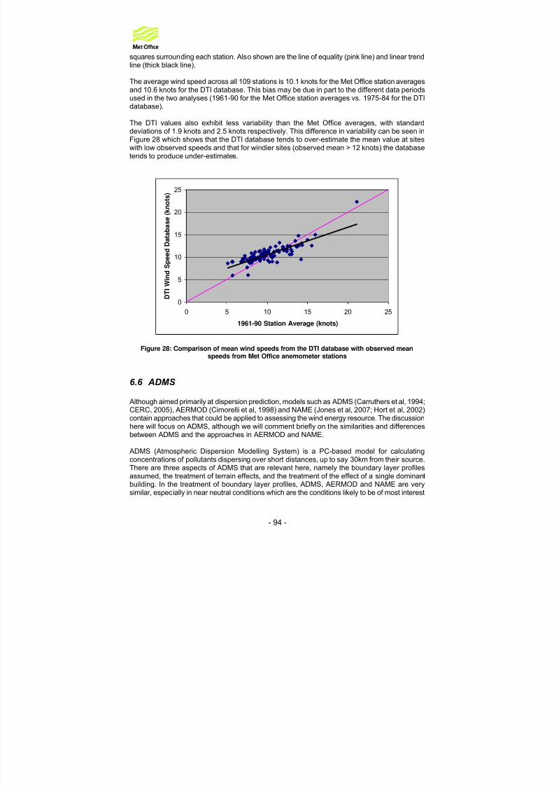
- 98 -
speeds are excluded from the MCP analysis (to improve the fit to the higher wind speeds of interest to wind energy studies) then the technique can produce biased predictions. Errors in theMCP predictions decrease as the monitoring period increases, but there still remains quite a lotof uncertainty in the results (demonstrated by using several different data periods of the samelength). The authors conclude that both techniques are capable of making useful predictions,although in complex terrain the uncertainties can be quite large, especially for MCP.
Frank & Landberg (1997) compare values from WAsP with results obtained by down-scalingdata from a mesoscale model (see §3.2.2 for more details of this technique). Given that themesoscale model cannot capture sub-grid scale effects, the comparison is made with WAsPpredictions for flat terrain and uniform roughness. The study area is the whole of Ireland. Theauthors find that the range of values in the mesoscale model predictions is less than that in theWAsP data. Reasonable agreement is obtained for windier sites but for sites with lower meanspeeds the mesoscale model tends to over-predict the available wind energy. The likelyexplanation for these differences is that the down-scaling process does not allow for situationswhen the surface wind flow is decoupled from the free atmosphere above e.g. due to atemperature inversion.
Suarez et al (1999) compare WAsP and MS-Micro/3 with a scoring system known as DAMS.DAMS was developed for forestry applications to allow the relative windiness of different sites tobe compared. It involves assigning a score to each of a number of geographic factors (climaticzone, aspect, elevation, exposure, terrain shape and orientation). An overall windiness score isdetermined by combining these individual scores together, based on their relative importance asdetermined from field experiments). The DAMS scores were converted to wind speeds byscaling them by the ratio of the observed mean speed and DAMS score at one particular locationin the study area (an area of complex forested terrain in Scotland). The authors found that allthree approaches produced variable results. The two linear models were most accurate onexposed hill tops whereas DAMS was more accurate in valleys and on lower slopes. Overall the
DAMS system was found to perform as well as the terrain flow models, despite a number of limitations (no surface roughness dependency or wind direction dependency). The DAMSwindiness scores have subsequently been calculated for the whole of the country. The authorssuggest that DAMS could potentially be used to correct the output from linear flow models.
Achberger et al (2002) compare the WAsP model with three versions of the MCP technique (seeprevious discussion in §6.2 and §6.3). The target site is a location in southern Sweden in flat,open terrain. They compare results from three different reference datasets – anemometer datafrom a nearby observing station, plus 10m and geostrophic winds from a mesoscale model. Interms of mean wind speed and the probability of speeds > 6 m/s, the best results were obtainedwith the WAsP model in combination with the anemometer data.
Landberg et al (2003) summarise eight methods for generating estimates of wind resources:folklore; the use of unadjusted measurements only; MCP; global re-analyses of NWP data(adjusted to the surface using the geostrophic drag law); the wind atlas methodology (i.e. the useof terrain flow models, such as WAsP, or even CFD, to correct surface observations for localeffects); the use of on-site measurements to drive terrain flow and CFD models; statistical-dynamical down-scaling of mesoscale model data; the use of terrain flow models to adjust theoutput from a mesoscale model. They do not consider geostatistical interpolation techniques.The authors identify four areas where estimation techniques need to be improved: in complexterrain; at offshore locations; for large heights above ground level; for sites in forest clearings.For sites in forested areas (arguably the most similar to urban locations, which are notmentioned) they note the need to take into account the displacement height, as well as speed-upand separation effects at clearing boundaries.

8/6/2019 Best Et Al._small-Scale Wind Energy Technical Report_2008
http://slidepdf.com/reader/full/best-et-alsmall-scale-wind-energy-technical-report2008 100/191
- 99 -
7 Siting Guidelines
In this section we consider the relative suitability of different possible small scale turbine
locations from the range of choices that would typically be available to a potential turbinepurchaser. In contrast to the situation for large turbine arrays, for small scale generation thepurchaser is not so much interested in where the best locations in the country are but where thebest locations are in the locality of his home. To assess the absolute suitability one would needalso to take account of wind strengths in the area using a method like that proposed in part twoof this report (Urban Wind Energy Research Project, Part 2: Estimating the Wind EnergyResource). We consider both urban and rural situations, although the main interest here is for urban wind power generation.
From a meteorological perspective, there are two main issues to bear in mind in siting a windturbine. These are that wind speed generally increases with height and that upwind obstructionstend to reduce wind speed and increase turbulence levels. High turbulence levels can reduce theeffectiveness of wind turbines. There are also some other meteorological issues which arise if one has a large area to choose from in siting the turbine and there are significant differences inthe character of the terrain across the area. In practice there will of course also be other non-meteorological issues to consider, such as the cost and safety of erecting and connecting theturbine, the ease and safety of maintenance, the noise and vibration from the turbine, andplanning permission. However we are not concerned with such issues here. Some of theseissues are discussed by BRE Certification Limited (2007) and Gipe (2004).
Turbine Height: We consider first the question of height. All else being equal, the turbine shouldbe mounted as high as possible. Wind speed generally increases with height according to thelog law:
0
* ln zd zu
u−
= κ (see section 4.1). As a result, the fractional increase in wind speed Δ u /u for a given fractionalincrease in height Δ z /z is given by:
0
ln1
1
zd z
zd z
zuu
−
−
×Δ≈Δ
This means that the advantages of increasing the height are larger over rough surfaces (such asurban areas and forests where z 0 and d are large) than they are over smoother areas. Note thatthe equation is only formally justified at heights well above the roughness elements (buildings,trees etc). However there is some evidence that in urban areas it works reasonably well inpractice down to near the top of the building “canopy”, although with somewhat more scatter andvariability from one location (in the horizontal) to another. The equation also assumes neutralconditions, but these are the most important when considering wind energy as the stability isnormally close to neutral in strong winds. The factor on the right hand side of the equation canbe estimated using typical values of z 0 and d as given, for built-up areas, in Table 4 in section4.1. For rural (non-built-up) conditions there are numerous tables of values available, especiallyfor z 0. The following values of z 0 are based on those used in the Met Office Unified Model andthe Met Office Surface Exchange Scheme II (MOSES II) (see Esseryet al . 2001):
Forests Shrubs Open country/Grass Water z 0 h / 20 ≈ 1 m h/10 ≈ 0.18 m 0.14 m 0.0003 m

8/6/2019 Best Et Al._small-Scale Wind Energy Technical Report_2008
http://slidepdf.com/reader/full/best-et-alsmall-scale-wind-energy-technical-report2008 101/191
- 100 -
Here h is the height of the trees or shrubs. The true roughness for short grass itself is rather smaller than given here, say about 0.03 m, but it is rare to have extensive grasslanduninterrupted by hedges, bushes etc, so the value given in the table is generally moreappropriate in practice (and is the value currently used in the Met Office Unified Model). Thedisplacement height d can be neglected in rural settings except for forests where it can beestimated as 2/3 of the height of the trees (Oke 1987, p116).
At heights below the top of the roughness elements the wind decreases rapidly with height andbecomes more turbulent (relative to the mean wind speed) and harder to predict. As a resultsuch locations should be avoided if possible. The estimates given in the second half of thisreport (Urban Wind Energy Research Project, Part 2: Estimating the Wind Energy Resource)show generally poor turbine performance is expected at heights just above the canopy top;within the canopy the results will be worse.
Note that, when we refer to roughness elements in the above, we have in mind the generalcharacter of the neighbourhood. For an isolated house in an open rural setting, the house wouldnot be included in the roughness elements but would be regarded as an “isolated obstruction”.
Obstructions: The second key issue to consider is obstructions to the wind flow. Obstructionsfall into two main types (with some overlap): those that form part of the general surroundingroughness (e.g. a house in an estate of similar houses) and those that protrude above thegeneral roughness and form more isolated obstructions (e.g. a tower block in an area of one or two storey housing). The obstructions which form part of the general roughness act collectivelyto slow the flow, but the effect of any one element is not very large. This is especially true asregards the flow above the roughness canopy where, for reasonably dense canopies, the flowtends to skim over the top of the canopy. In contrast the obstructions which protrude above thegeneral roughness generally have a much larger effect, especially in the case of buildings. They
can cause substantial vertical motions up and down the front face of the building, largeseparation and wake regions, and downwash behind the building (see section 5.1.3). The reasonfor the difference is primarily because in the former case the flow is already substantially slowedwithin the canopy by the other roughness elements. Hence the energy and momentum of theflow within the canopy is low and, even when deflected by obstacles, is insufficient tosubstantially affect the flow above the canopy. The CFD study by Heathet al . (2007 – seeespecially figures 9 and 10) shows clearly the different character of the flow around a building inthe two cases.
Of course in reality obstructions form a continuum between those which are clearly embeddedwithin a canopy and those that are more isolated. At one extreme we have, for example, a lowdensity rural environment where the spacing between buildings may be large enough that theflow, after being disturbed by one building, has time to reach equilibrium with the ground beforeencountering another building. At the other extreme we have the narrow street canyon where thesize of the recirculation behind one row of buildings is constrained in size by a second row. Inbetween we have situations where the separated flow behind a building reattaches, but wherethe next building lies within the low velocity wake of the first building.
As a rough rule of thumb we regard an obstruction as being part of the general canopy if thereare a number of other obstacles of similar or greater height nearby with at least one within ahorizontal distance of 5-10 times the obstacle height. A certain amount of judgment and commonsense is needed in applying this, e.g. one might in the case of trees, regard a small clump of trees as a single obstacle. The basis for this criterion is as follows. The typical length of therecirculation region behind an isolated building (see section 5.1.3) is between 3 and 12 times thebuilding height. Also the street canyon results of Siniet al . (1996) show that the street canyonvortex splits into two and eventually reattaches as the street width increases from 5 to 9 times

8/6/2019 Best Et Al._small-Scale Wind Energy Technical Report_2008
http://slidepdf.com/reader/full/best-et-alsmall-scale-wind-energy-technical-report2008 102/191
- 101 -
the building height. The length of the wake region behind an obstacle can of course be muchlonger than the recirculation region, but that length is more relevant as a criterion for there to besome influence of one building on the next rather than for the obstacles to form a canopy. Oke(1987, p266) gives a somewhat lower spacing of about 3 times the building height for therecirculation regions behind and in front of buildings to collide (he calls separations greater thanthis “isolated roughness flow”, although this does not mean that there is no interaction betweenthe far wake beyond the recirculation region and the next building).
Obstructions forming part of the canopy: We consider obstructions which form part of thegeneral canopy first. Because the flow tends to skim over the top of the canopy the effect, on aturbine mounted above the roof tops, of any individual roughness element is likely to be small.There is no particular reason to take such obstacles into account in siting the turbine, althoughthere will of course be a general reduction in wind speed from their collective effect. Thisconclusion will be less reliable the closer one is to the canopy top. However even here there islittle likelihood of being able to predict departures from the horizontally averaged wind without adetailed site-specific study, for example in a wind tunnel or through wind speed measurementsat possible siting locations. This is because the effects will depend on the detailed geometry of anumber of the obstructions. Also the results will vary with wind direction and in general we wouldexpect there to be no location at the height of interest which is preferred for all wind directions.
If the location is below the height of the obstacles then the situation is different. The wind speedin general at such heights will be reduced and the effects of the roughness elements will vary asthe turbine location varies in the horizontal plane at the height of interest. In particular there is adanger of encountering recirculating flows. The primary advice must be to mount the turbinehigher if at all possible. However if this is not possible then one should choose a location with asmuch unobstructed view as possible in the direction from which the prevailing wind blows. As inthe case of locations close to the top of the canopy, the results will in general be hard to predictwithout detailed study. However unlike the former situation, the effects of the precise siting will
be more important.The CFD study of Heathet al . (2007) shows examples where the ‘maximum unobstructed view’approach is not optimal for a turbine at or below the canopy top. This illustrates the difficulty of making reliable general rules for such situations. They consider possible mounting locations on adetached pitched roof house in an array of similar houses. When considering mounting belowthe maximum roof height they find that for some wind directions the optimal location is at thedownwind corner. Unfortunately they only give the wind speed at the optimal location so it is notpossible to compare with that at other locations. However in such locations the performance maybe compromised by turbulence and we would not recommend such locations without detailedsite-specific study.
Isolated obstructions: We now consider isolated obstacles. These can produce effects over large areas. In the case of buildings the effects can extend up to 2-3 times the obstacle heightabove the ground (more for buildings with width much greater than height) and up to 30 timesthe building height in the downwind direction, although for buildings with strong roof topgenerated vortices the wake can persist further downwind (see sections 5.1.3 and 6.6). Theupwind extent of the influence is generally small.
We note also the guidance for making meteorological wind observations given by the Met Office(2000). These say the ideal is open terrain with no obstructions within 300m. However if thereare significant obstructions they recommend raising the anemometer to at least the height of theobstacle and sometimes more, depending on the size and distance of the obstacle. If the wind ismeasured by a mast on a roof top, they recommend a measurement height of at least half andideally three-quarters of the building height above the roof. In practice it may be impossible tomeet these high standards in siting turbines and avoid any influence from such obstructions.

8/6/2019 Best Et Al._small-Scale Wind Energy Technical Report_2008
http://slidepdf.com/reader/full/best-et-alsmall-scale-wind-energy-technical-report2008 103/191
- 102 -
However it should be remembered that even small effects on wind speed can have a significanteffect on power output. Isolated trees or groups of trees and hedges are likely to have effects onthe flow which are similar to but somewhat smaller than buildings of the same size (see section5.1.3).
As a result of the above, the primary guidance must be to put the turbine as far away from suchobstacles as is practical, especially when the obstacle is in the upwind direction relative to theprevailing wind direction. This should ideally be either 30 obstacle heights downwind or 2-3obstacle heights above ground. In many cases this will be impractical and compromises will berequired. However, if this is the case, one should try to ensure that one is well outside anyrecirculation region behind the obstacle, at least for obstacles which are upwind for the prevailingwind. This region can be regarded as extending to typically 3-10 building heights downwind, withthe larger values being applicable to obstacles for which the width is large compared to theheight (see section 5.1.3). The height of the recirculation is more complex to assess. It is at leastequal to the height of the obstacle, but may be deeper, say 1.5 times the building height, for buildings that have pitched roofs (see simulations in Heathet al . (2007)) or whose along winddimension is short enough for roof top reattachment not to occur (see section 5.1.3).
Separate considerations are needed if the turbine is to be mounted directly on a building whichconstitutes an isolated obstruction. For flat roofed buildings, the height above the roof shouldexceed the height of any roof top recirculation region or wake region. This can be estimated as0.28 min(W B
7/9H B2/9, W B
5/9H B4/9) using the results of Wilson (1979) – see section 5.1.3. Here W B is
the maximum of the length and width of the building andH B is the height of the building. For pitched roof buildings, one should again aim to keep the turbine out of the recirculation region.We do not have a lot of evidence to say what this requires in terms of mounting position.However, based on the isolated building simulation by Heath et al . (2007), we propose thefollowing. The turbine should be mounted at least half the height of the roof (i.e. half the verticaldistance from the roof base to peak) above the peak, or should be mounted at or in front of the
peak from the perspective of the prevailing wind direction (and ideally both).In some situations the wind speed can be enhanced by flow over buildings. However it is difficultto exploit this without a detailed site-specific study. The speed up is likely to be restricted to acertain range of wind directions and may be associated with significant vertical motions or increased turbulence which may reduce or eliminate the benefit, even for the directions which doyield a speed up.
Larger scale terrain variations: If there is a wide area over which the turbine could be located,such as may be the case on farms or large estates or where someone is fine tuning their choiceof where to live based on the potential for wind power, then there are additional considerationsthat arise. For example it is appropriate to choose areas where the general character of the area
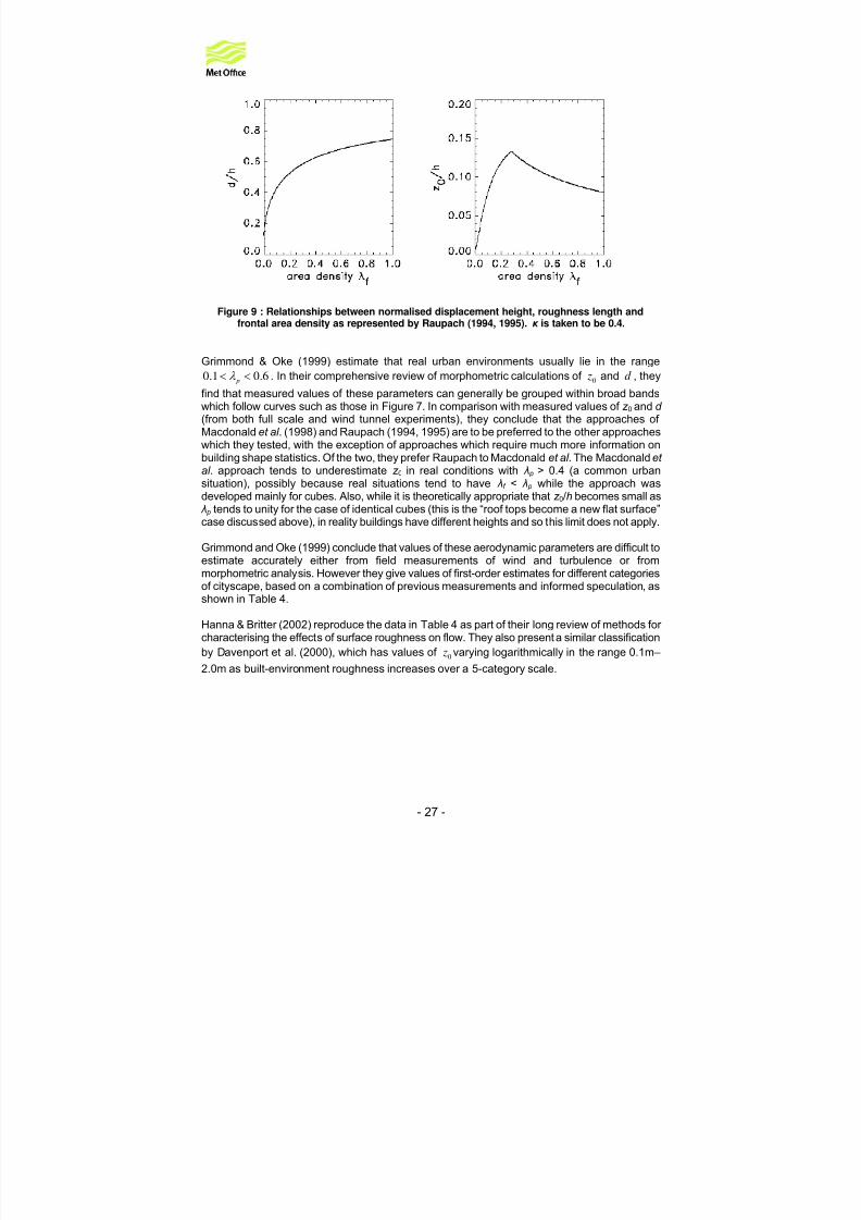
is as smooth as possible, preferring e.g. open grassland to forested areas.This is not just a question of obstructions – an unobstructed location above a rough area such asa forest will generally experience substantially lower wind speeds than are found at the sameheight over a smooth surface such as grass. In principle there is an exception where the rougher area is too small to affect the wind at the turbine height. However unless the turbine is especiallyhigh or the rough area very small (in which case it may be better regarded as an obstruction) thisis unlikely to be relevant in practice (see Figure 9 and note that, for the relevant part of the graphnear the origin, the growth of the internal boundary layer is rapid; in addition there isconsiderable uncertainty in the initial growth with complications due to displacement heights andvertical motions generated as the flow decelerates).
In general one should regard a region as rougher if the roughness elements are taller or moredensely packed. However this is not universally true. If the roughness elements are all of a

8/6/2019 Best Et Al._small-Scale Wind Energy Technical Report_2008
http://slidepdf.com/reader/full/best-et-alsmall-scale-wind-energy-technical-report2008 104/191
8/6/2019 Best Et Al._small-Scale Wind Energy Technical Report_2008
http://slidepdf.com/reader/full/best-et-alsmall-scale-wind-energy-technical-report2008 105/191
- 104 -
• For a turbine mounted on a flat roof building that protrudes above the general level of theroughness elements:
o Try to ensure that the turbine height above the roof is at least 0.28 min(W B7/9H B
2/9,W B
5/9H B4/9) where W B is the maximum of the length and width of the building and
H B is the height of the building• For a turbine mounted on a pitched roof building that protrudes above the general level
of the roughness elements:o Try to ensure that either the turbine height above the roof peak is at least half the
vertical depth of the roof (base to peak)or the turbine is mounted at or in front of the peak from the perspective of the prevailing wind direction (and ideally both)
• Locate the turbine over a rural, non-forested area in preference to built up or forestedareas
• If in a built up or forested area, locate the turbine near the edge of the area and near thepoint on the edge of the area that is upwind of the area from the perspective of theprevailing wind
• Locate the turbine near the top of smoothly varying hills, but be cautious about sharply
varying terrain (e.g. cliff tops may be very turbulent; also if the terrain is steep one shouldbe right at the top or, if this is impossible, on the upwind side of the top from the point of view of the prevailing wind direction).
These guidelines are illustrated in somewhat simplified form in Figure 29. We note that it isimpossible for these guidelines to cover all possibilities and that, to interpret the guidelinesappropriately in a complex situation, it is useful to understand the motivation for the guidelines.Also, especially when there are obstructions to the flow, results may not be very predictablewithout a detailed site-specific study, for example in a wind tunnel or through wind speedmeasurements at possible siting locations.
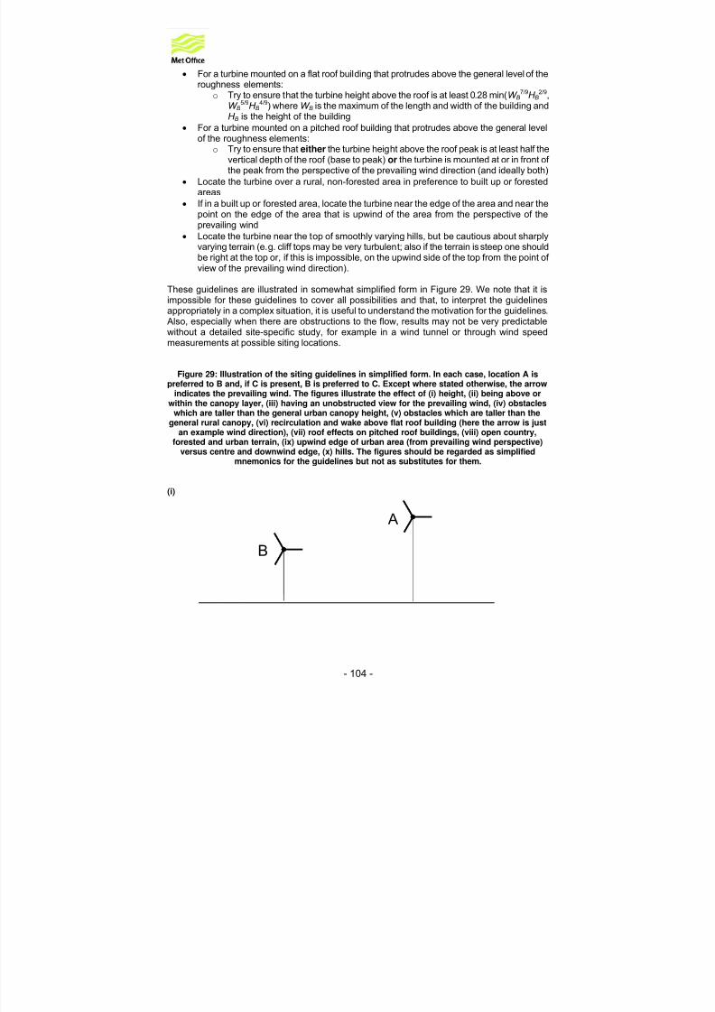
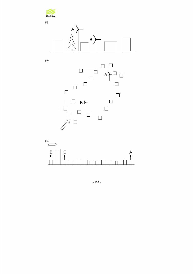
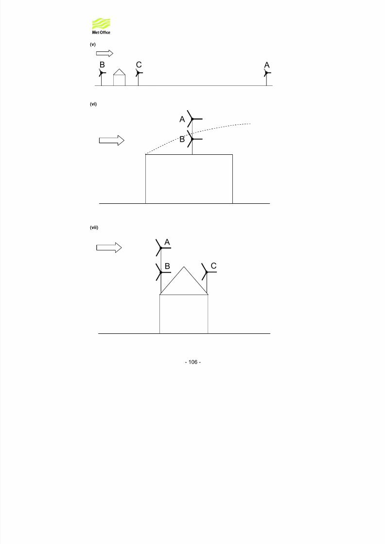
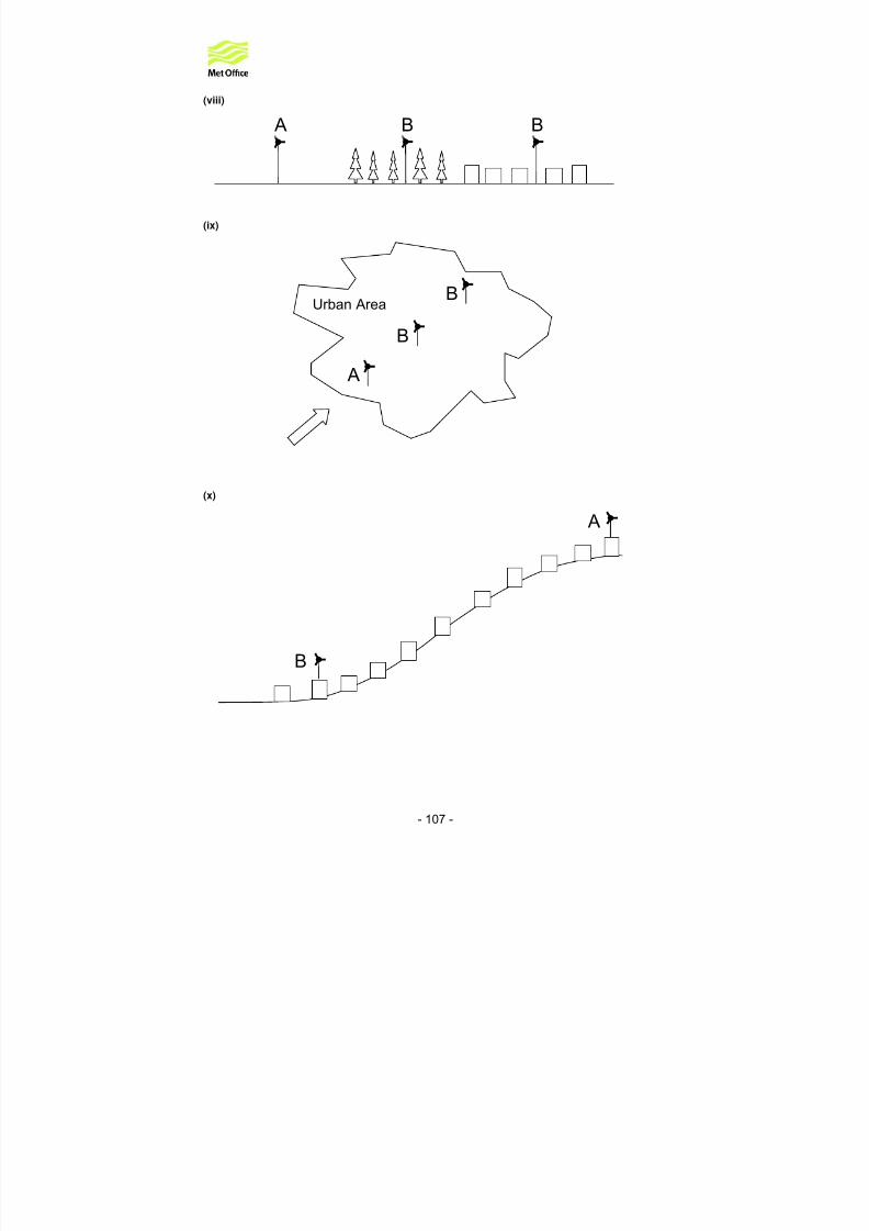
Figure 29: Illustration of the siting guidelines in simplified form. In each case, location A ispreferred to B and, if C is present, B is preferred to C. Except where stated otherwise, the arrowindicates the prevailing wind. The figures illustrate the effect of (i) height, (ii) being above or
within the canopy layer, (iii) having an unobstructed view for the prevailing wind, (iv) obstacleswhich are taller than the general urban canopy height, (v) obstacles which are taller than the
general rural canopy, (vi) recirculation and wake above flat roof building (here the arrow is justan example wind direction), (vii) roof effects on pitched roof buildings, (viii) open country,
forested and urban terrain, (ix) upwind edge of urban area (from prevailing wind perspective)versus centre and downwind edge, (x) hills. The figures should be regarded as simplified
mnemonics for the guidelines but not as substitutes for them.
(i)
A
B
8/6/2019 Best Et Al._small-Scale Wind Energy Technical Report_2008
http://slidepdf.com/reader/full/best-et-alsmall-scale-wind-energy-technical-report2008 106/191
- 105 -
(ii)
A
B
(iii)
A
B
(iv)
AB C
8/6/2019 Best Et Al._small-Scale Wind Energy Technical Report_2008
http://slidepdf.com/reader/full/best-et-alsmall-scale-wind-energy-technical-report2008 107/191
- 106 -
(v)
B C A
(vi)
A
B
(vii)
A
CB
8/6/2019 Best Et Al._small-Scale Wind Energy Technical Report_2008
http://slidepdf.com/reader/full/best-et-alsmall-scale-wind-energy-technical-report2008 108/191

8/6/2019 Best Et Al._small-Scale Wind Energy Technical Report_2008
http://slidepdf.com/reader/full/best-et-alsmall-scale-wind-energy-technical-report2008 109/191
- 108 -
8 Summary
Chapter 2 – Conventional Surface Observations
The Met Office anemometer network includes a number of sites in urban areas. However few, if any, have exposures that are typical of urban wind turbines.
Long-term averages of wind speed have been calculated for 1961-1990 and 1971-2000 for thesites in the Met Office observing network.
The 2-parameter Weibull distribution is widely used for modelling the wind speed frequencydistribution. The acceptance of this as the only distribution to use is questioned by someresearchers.
Chapter 3 – Atmospheric Models
Conceptually the atmosphere can be represented by a number of layers i.e. free atmosphere,boundary layer, inertial sublayer, roughness sublayer, canopy layer. Different processesdominate in each layer, but the layers are nevertheless interdependent i.e. each layer influences,and is influenced by, the adjacent layers. The urban boundary layer has a particularly complexstructure involving wide variations in time and space.
The wind speed in the free atmosphere is proportional to the horizontal pressure gradient.Climatologies of wind speed at levels above the boundary layer can be obtained in a number of ways e.g. from surface pressure data, from radiosonde data, or by correcting surface wind data.
The winds nearer the surface are driven by, and vary with, the wind in the free atmosphere. Instrong wind conditions the effects of heating and cooling of the atmosphere are not significantand over uniform terrain the vertical profile of wind speed has a logarithmic shape. However therelationship in general is complex and time-varying. Even in simple situations (neutral stabilityand open terrain) it is difficult to predict the surface wind to within 10% purely from the windspeed in the free atmosphere.
Operational weather forecast models (NWP) and reanalyses are important sources for thederivation of climatologies of wind speed and direction at heights above the boundary layer. Themajor drawback of reanalyses is the relatively coarse horizontal resolution of 100-200kmcurrently available. Finer scale (~10km) climatologies have been derived by a variety of methods: statistical, statistical-dynamical and dynamical adaptation, which are increasingly
expensive in computation and processing. To reduce costs a smaller set of finer-scale modelsimulations are performed based on a classification of the reanalyses into classes.
Operational NWP limited area models offer a more direct approach by forming means of the pastweather forecasts of wind. These are currently available at ~10km resolution. The advantagesare that the computing cost of dedicated simulations is saved and potentially all weather regimesand transitions may be sampled to produce a consistent and comprehensive climatology. Apossible disadvantage is that the models have evolved over time and so the accuracy of the datais not uniform over long periods.
Chapter 4 – Boundary Layer Models
Urban areas are represented in numerical models at various levels of complexity. The simplestmodels characterise urban areas as homogeneous regions. Others resolve detail within built-up

8/6/2019 Best Et Al._small-Scale Wind Energy Technical Report_2008
http://slidepdf.com/reader/full/best-et-alsmall-scale-wind-energy-technical-report2008 110/191

8/6/2019 Best Et Al._small-Scale Wind Energy Technical Report_2008
http://slidepdf.com/reader/full/best-et-alsmall-scale-wind-energy-technical-report2008 111/191
- 110 -
In more complex situations with many buildings, wind tunnel experiments or numericalsimulations offer a tool to understand the flow in detail. However there is still a need to test suchapproaches against full scale measurements.
There are a number of full scale field studies that have been conducted to help understandurban flows. Results from DAPPLE (Marylebone Road), Salford, Birmingham and MUSTexperiments have been discussed. The last of these is a field trial, although not full scale,consisting of a mock urban setting constructed from shipping containers. Field experiments inBirmingham and Salford showed that wind speeds at 15m above ground in a built-up area canbe 20% less than those at 10m above ground in open terrain. Also the variations of wind speedwith height above ground level can be approximated by a simple power law. The experimentsalso showed that estimates of surface roughness can be derived from land use data together with estimates of the upwind fetch over which the surface influences a given measurement.
Chapter 6 – Applied Tools
Geostatistical interpolation techniques have been used to interpolate station long-term averagesonto a 1km grid. However these grids do not attempt to capture the effects of urban areas on themean wind speed.
The measure-correlate-predict (MCP) technique estimates the wind climatology of a target siteby using the statistical relationship between concurrent observations from the target site and anearby reference site to correct the reference site climatology. There is no practical reason whythe MCP method could not be applied to urban locations – a sample calculation for a site in thecentre of Norwich suggested that satisfactory results can be obtained. However the skill of thetechnique depends on the statistical correlation between the target site and reference stationand it seems likely that this will be lower for typical turbine locations than for more exposed sites.
WAsP can model the effects of urban areas, but only as regions of homogeneous surfaceroughness. The shelter model treats obstacles in a fairly simple way and is only applicable atsome distance from the obstacle (at least five times the obstacle height). WAsP is unable tomodel the details of the wind flow close to buildings and other obstacles. The WAsP softwarehas been used to estimate the wind climatology in a wide range of situations including offshorelocations and complex terrain. There do not appear to be any published studies relating directlyto the wind climatology of urban areas.
Proprietary software packages used by the wind energy industry (e.g. WindFarmer, WindFarmand WindPRO) make direct or indirect use of several techniques for modelling the wind climate.These include boundary layer flow models (WAsP, MS-Micro/3), MCP and CFD.
The 1961-1990 station averages have been used to assess the 10m data from the DTI WindSpeed Database. The DTI Database tends to over-estimate the mean wind speed at sites withlow observed averages and under-estimate the mean at sites with higher observed averages.
Models for the dispersion of pollutants such as ADMS, AERMOD and NAME contain algorithmsfor describing the flow which have potential for application to wind energy problems. For example, ADMS includes (i) parametrizations of boundary layer wind and turbulence profilesover homogeneous terrain above the roughness sublayer, (ii) a linear flow model for predictingterrain effects on the flow, and (iii) a model which predicts aspects of the flow around isolatedbuildings (although this does not provide a complete flow field).
Various inter-comparisons of WAsP, MCP, NOABL and down-scaling of NWP models have beenpublished. These shed some light on the relative strengths and weaknesses of the different

8/6/2019 Best Et Al._small-Scale Wind Energy Technical Report_2008
http://slidepdf.com/reader/full/best-et-alsmall-scale-wind-energy-technical-report2008 112/191
- 111 -
approaches, however none of the studies relate specifically to the problem of predicting windspeeds in urban areas.
Chapter 7 – Siting Guidelines
Drawing on the information contained in the preceding chapters, an assessment has been madeof the relative suitability of different locations for small-scale wind turbines. Consideration hasbeen given to positioning both pole-mounted and roof-mounted turbines. The key factors toconsider are the height of the turbine and the influence of upwind obstacles. Guidelines havebeen produced covering a variety of common situations.

8/6/2019 Best Et Al._small-Scale Wind Energy Technical Report_2008
http://slidepdf.com/reader/full/best-et-alsmall-scale-wind-energy-technical-report2008 113/191
- 112 -
9 Conclusions
The aim of this first phase of the project has been to examine the range of existing data sources,
analysis techniques and tools that might be used to a) clarify the performance of small-scalewind turbines in urban areas, and b) clarify how turbines should be sited for maximum carbonsavings. The following conclusions are drawn:
The extent of data available to describe wind conditions in urban areas:
• There are a variety of sources of wind speed and direction data available, includinganemometer data (both routine measurements and from field trials), NWP data andreanalysis data.
• All of these data types have limitations, either in terms of their temporal or spatial extent,or in terms of their representativity of urban areas.
• Any of these data sources could, in principle, be used to estimate wind conditions inurban areas if combined with appropriate interpolation, correction or downscalingtechniques.
• There are no existing datasets from which it would be possible to estimate directly thetotal UK wind energy resource from micro-generation.
The state of the art in predicting wind conditions in urban areas:
• There are a range of techniques available for predicting wind conditions near the surface,including NWP models (with or without downscaling), linear flow models (e.g. WAsP),
simple analytic models of fetch effects and roughness changes, MCP, geostatisticalinterpolation, mass consistent models (e.g. NOABL) and CFD.• These techniques have applications in a wide variety of situations e.g. weather
forecasting (NWP models), climate monitoring (geostatistical interpolation), pollutantdispersion modelling (linear flow models), wind farm siting (linear flow models, MCP,mass consistent models), modelling fluid flow (CFD).
• None of these techniques have been developed specifically for predicting windconditions in urban areas.
• Through the use of appropriate input data, combination of techniques, model tuning andcalibration, any of these techniques could be used to predict urban wind conditions.
• Note that there are practical limitations associated with using some of these techniquesto generate predictions over a large area such as the UK e.g. the amount of dataprocessing that would be required, issues associated with ensuring the predictions varysmoothly and consistently over the analysis area etc.
Applicability of techniques developed for large-scale wind farms:
• None of the principal data sources or analysis techniques used for siting large-scale windfarms was developed with urban wind energy generation in mind.
• The DTI Wind Speed Database (created using the NOABL model) does not reflect theeffects of urban areas (the wind speed values are representative of open, level terrain).
• The WAsP model can describe the large-scale effects of areas of high surface
roughness (such as urban areas) but is not designed to model the wind flow close tobuildings.

8/6/2019 Best Et Al._small-Scale Wind Energy Technical Report_2008
http://slidepdf.com/reader/full/best-et-alsmall-scale-wind-energy-technical-report2008 114/191
- 113 -
• The MCP technique can be applied to urban locations although the quality of thepredictions depends on the level of correlation with the reference site. However, giventhe need to gather data from the target site (and that in urban areas these data will berepresentative of a very limited area), this is not a practical technique for estimating windconditions over large areas.
• Tools such as WindFarmer, WindFarm and WindPRO do not include any functionalitydesigned specifically for siting turbines in urban areas.
Siting of turbines:
• For maximum efficiency, turbines should be sited as high as possible and away from anyobstructions (particularly in the prevailing wind direction).
• General guidelines on siting have been given for a number of idealised situations(including some specific recommendations for how high, or how far from an obstacle, aturbine should be sited).
• However, in many real situations (particularly in urban areas) there will be severalcompeting factors to consider and/or the exposure of the site will be very complex. For such locations it is likely that a detailed site-specific study will be required to determinethe optimal position for a turbine.
The second part of this report (Urban Wind Energy Research Project, Part 2: Estimating theWind Energy Resource) will examine how estimates of the UK energy resource from small-scaleturbines can be derived using the available analysis techniques and data sources.

8/6/2019 Best Et Al._small-Scale Wind Energy Technical Report_2008
http://slidepdf.com/reader/full/best-et-alsmall-scale-wind-energy-technical-report2008 115/191
- 114 -
10 Glossary
Boundary layer – That part of the atmosphere that is adjacent to the Earth’s surface and which is
affected by the properties of that surface.Canopy layer or sublayer – The part of the atmospheric boundary layer occupied by theroughness elements (buildings in the urban case).
Fetch – The area upwind of a site, over which the air has travelled.
Flow separation – The process by which an eddy forms on the windward or leeward sides of bluff objects or steeply rising hillsides.
Flux – Rate of transport.
Hydrostatic equilibrium – The state of balance between the force of gravity and the verticalcomponent of the pressure gradient force. It is a state of the atmosphere in which there is novertical acceleration of the air.
Inertial sublayer – The part of the atmospheric boundary layer that is much lower than theboundary layer depth but much higher than the surface roughness elements.
Morphometric – Based on the form of the surface i.e. based on the dimensions and distributionof roughness elements.
Obukhov length – A quantity that characterises the relative importance of mechanically andthermally produced turbulence.
Roughness layer or sublayer – The part of the atmospheric boundary layer that is not muchhigher than the surface roughness elements.
Surface layer – For the large scale meteorological community, this is synonymous withinertial sublayer . However the urban meteorological community often uses the term to mean the inertial sublayer and roughness sublayer combined.

8/6/2019 Best Et Al._small-Scale Wind Energy Technical Report_2008
http://slidepdf.com/reader/full/best-et-alsmall-scale-wind-energy-technical-report2008 116/191
- 115 -
11 List of Symbols
LATIN
a Constanta, b, ca1, b1, c1 a2, b2, c2
Empirical constants in linear regression equations (MCP analysis)
a Decay constant for exponential canopy wind profile A Weibull scale parameter A,B,C Empirical constants (different in different equations).
F A Frontal area of roughness element
P A Plan area of roughness element
T A Total plan area of roughness element and surrounding spaceb Constant
T B turbulent buoyancy fluxc Empirical constant in IBL relationship.
d C Bulk building drag coefficient.
d c Sectional building drag coefficient.Cn Wind speed, height n metres, Coleshill site, n=10, 15, 30, 45
i D Canopy drag.
y D , z D Crosswind and vertical source weight distributions.Dn Wind speed, height n metres, Dunlop Tyres Ltd site, n=10, 15, 30, 45d Zero plane displacement height.
1E () First E n
f Coriolis parameter.G Geostrophic wind.g Acceleration due to gravity.
H equilibrium boundary layer depth according to Rossby similarity theory.H B Building or street canyon heightH h Hill height. H δ Sensible heat flux at the top of the internal boundary layer.
s H Surface sensible heat flux.h Mean building height (or canopy height).
hBL Height of boundary layer k Wavenumber (of surface heterogeneity) = 2π λ .k Turbulent kinetic energy per unit mass (used mainly in the phrase “ ε -k
model”)k Weibull shape parameter L Obukhov length.
B L Building length
h L Hill width at half height.
R L Length scale of each region of roughness for heterogeneous surface.
c L Canopy-drag length scale.l Turbulent length scale.

8/6/2019 Best Et Al._small-Scale Wind Energy Technical Report_2008
http://slidepdf.com/reader/full/best-et-alsmall-scale-wind-energy-technical-report2008 117/191
- 116 -
bl Blending height.l c Mixing length
d l Diffusion height.
il Inner region depth.
0l Internal boundary layer depth scale. M Roughness change parameter, ( )02 01ln M z z= .
c N Canopy adjustment number.P x Magnitude of horizontal pressure gradientp Constant in source area model. p Power (exponent) in simple wind profile power lawr Correlation coefficientr mean Mean value of the ratio of the concurrent wind speeds at a reference
station and a target site in an MCP analysiss Constant in source area modelsr Standard deviation of the ratio of the concurrent wind speeds at a
reference station and a target site in an MCP analysisvu ss , Standard deviations of the concurrent data at a reference station and a
target site in an MCP analysisT Temperature.
T Δ Urban-rural temperature difference.T Δ Difference between the air temperatures at two heights at a reference
station (MCP analysis)t Time.
AU ‘Large scale’ or ‘Rural’ wind speed at reference height . A z
cU Representative wind speed within the urban canopy
H U Wind speed at building heightiU In-canopy wind speed.
U , V Wind speed( )u z Wind speed profile.
( )ref u z Reference wind speed profile.'( )u z Perturbation wind speed profile.
0u Internal boundary layer velocity scale.
1u Wind speed at height 1 z
2u Wind speed at height 2 z
*u Friction velocity.
*1u , *2u Friction velocity upstream (1) and downstream (2) of a roughness change.
iu The i th component of the velocityu, v Wind speeds at a reference station and a target site (MCP analysis)u x, v x Easterly component of wind speed at a reference station and a target siteu y, v y Northerly component of wind speed at a reference station and a target site
vu , Mean values of the concurrent data at a reference station and a target sitein an MCP analysis
x Distance along wind direction (e.g. from edge of urban area). y Distance perpendicular to wind direction
BW Building widthWS Street canyon width

8/6/2019 Best Et Al._small-Scale Wind Energy Technical Report_2008
http://slidepdf.com/reader/full/best-et-alsmall-scale-wind-energy-technical-report2008 118/191
- 117 -
z Height (above ground).( ) z x Mean plume height.
A z Reference height for ‘large scale’ or ‘rural’ wind.
0 z Roughness length.
01 z , 02 z Roughness length upstream (1) and downstream (2) of a roughnesschange.
0 A z Roughness length for ‘Large scale’ or ‘Rural’ wind . AU
0eff z Effective roughness length of aggregated surface.* z Height of the urban roughness sub-layer
H z Average height of buildings and other roughness elements Z Non-dimensional height (within urban roughness sub-layer)
GREEKα The angle between the top-of-boundary layer wind and surface stress. β Drag coefficient modification parameter for building arrangement.
v β Volume of canopy occupied by buildings.γ Euler’s constant, 0.577216.δ Internal boundary layer depth.
uΔ Cross-wake averaged velocity deficit behind a buildingε Rate of dissipation of turbulent kinetic energy per unit mass (used mainly
in the phrase “ ε -k model”)κ Von Karman’s constant (0.4).λ Wavelength (of surface heterogeneity).
eqλ Roughness density AND plan-area density, when these are assumed tobe equal
f λ Roughness density, i.e. total frontal area of buildings per unit ground area.
pλ Plan-area density.
sλ Mean building height to street width aspect ratio.ν Kinematic viscosity. ρ Air density.
wvu σ σ σ ,, Standard deviation of the turbulent velocity fluctuations in the along wind,across wind and vertical directions
yσ Gaussian plume width.τ Turbulent stress; local Reynolds stress.
advτ Advection timescale.Φ Latitude( )h z LΦ Monin-Obukhov stability function for heat
( / )m z LΦ Monin-Obukhov stability function for momentum
( ) z LΨ Monin-Obukhov stability function.
Ω Rate of rotation of Earth.

8/6/2019 Best Et Al._small-Scale Wind Energy Technical Report_2008
http://slidepdf.com/reader/full/best-et-alsmall-scale-wind-energy-technical-report2008 119/191
- 118 -
12 References
Abild, J, Application of the wind atlas method to extremes of wind climatology, Riso-R, NO. 722,Roskilde, Riso Natl.Lab. (1994)
Abramowitz, M. and Stegun, I. A. (Eds.). "Exponential Integral and Related Functions." Ch. 5 inHandbook of Mathematical Functions with Formulas, Graphs, and Mathematical Tables, 9thprinting. New York: Dover, pp. 227-233, 1972.
Achberger, C, Ekstrom, M and Barring, L, Estimation of local near-surface wind conditions - acomparison of WASP and regression based techniques, Meteorological Applications , 9 (2), 211-221 (2002).
Agnew, M.D., Palutikof, J.P., GIS-based construction of baseline climatologies for theMediterranean using terrain variables., Climate Research , 14 (2), 115-127 (2000)S.Arnold, H.ApSimon, J.Barlow, S.Belcher, M.Bell, D.Boddy, R.Britter, H.Cheng, R.Clark,R.Colvile, S.Dimitroulopoulou, A.Dobre, B.Greally, S.Kaur, A.Knights, T.Lawton, A.Makepeace,D.Martin, M.Neophytou, S. Neville, M.Nieuwenhuijsen, G.Nickless, C.Price, A.Robins,D.Shallcross, P.Simmonds, R.Smalley, J.Tate, A.Tomlin, H.Wang, P.Walsh, Dispersion of Air Pollution & Penetration into the Local Environment – DAPPLE,Science of the Total Environment , 332 , 139-153 (2004)
Arya S.P.S. and Wyngaard, J.C., Effect of baroclinicity on wind profiles and the geostrophic draglaw for the convective planetary boundary layer,J. Atmos. Sci. , 32 , 767-778 (1975)
Ayotte, K.W. and Taylor, P.A., A mixed spectral finite-difference 3D model of neutral planetaryboundary-layer flow over topography.J. Atmos. Sci. , 52 , 3523-3537 (1995)
Ayotte, K.W., Xu, D. and Taylor, P.A., The impact of turbulence closure schemes on thepredictions of the mixed spectral finite-difference model for flow over topography,Bound.-Layer Met. , 68 , 1-33 (1994)
Belcher, S. E., Jerram, N. and Hunt, J. C. R., Adjustment of a turbulent boundary layer to acanopy of roughness elements, J. Fluid Mech ., 488 , 369-398 (2003)
Barlow, J. F. and Belcher, S. E., A wind tunnel model quantifying fluxes in the urban boundary
layer, Boundary-Layer Meteorol. , 104 , 131-150 (2002)Barlow, J. F., Harman, I. N. and Belcher, S. E., Scalar fluxes from urban street canyons. Part I.Laboratory simulations. Part II. Model,Boundary-Layer Meteorol. , 113 , 369-410 (2004)
Barlow, J.F., Rooney, G.G., von Hunerbein, S. & Bradley, S.G., Relating urban boundary layer structure to upwind terrain for the SALFEX campaign,Boundary-Layer Meteorol. , in submission(2007)
Barnard, J.C., An evaluation of three models designed for siting wind turbines in areas of complex terrain, Solar Energy , 46 (5) , 283-294 (1991)

8/6/2019 Best Et Al._small-Scale Wind Energy Technical Report_2008
http://slidepdf.com/reader/full/best-et-alsmall-scale-wind-energy-technical-report2008 120/191
- 119 -
Barthelmie, RJ, Courtney, MS, Hojstrup, J, Larsen, SE, Meteorological aspects of offshore windenergy: observations from the Vindeby wind farm,Journal of Wind Engineering and Industrial
Aerodynamics , 62 (2-3), 191-211 (1996)
Basumatary, H., Sreevalsan, E., Sasi, K.K., Weibull parameter estimation: a comparison of different measures, Wind Engineering , 29 (3), 309-315 (2005)
Belcher, S.E., Xu, D.P. and Hunt, J.C.R., The response of the turbulent boundary layer toarbitrarily distributed roughness changes, Q. J. R. Meteorol. Soc. , 116 , 611-635 (1990)
Beljaars, A.C.M., Walmsley, J.L. and Taylor, P.A., A mixed spectral finite-difference model for neutrally stratified boundary-layer flow over roughness changes flow over topography,Bound.-Layer Met. , 38 , 273-303 (1987)
Bentham, T. and Britter, R., Spatially averaged flow within obstacle arrays, Atmos. Environ. , 37 ,2037-2043 (2003)
Best, M. J., Representing urban areas within operational numerical weather prediction models,Boundary-Layer Meteorol. , 114 , 91-109 (2005)
Best, M. J., Grimmond, C. S. B. and Villani, M. G., Evaluation of the urban tile in MOSES usingsurface energy balance observations, Boundary-Layer Meteorol. , 118 , 503-525 (2006)
Bornstein, R. and Lin, Q., Urban Heat Islands and Summertime Convective Thunderstorms inAtlanta: Three Case Studies, Atmos. Environ ., 34 , 507-516 (2000)
Borresen, J.A., Wind atlas for the North Sea and the Norwegian Sea, Norwegian Met. Inst.(Norw.Univ.Press), Oslo, 8200352765 (1987)
Botta, G, Castagna, R, Borghetti, M, Mantegna, D, Wind analysis on complex terrain - The caseof Acqua Spruzza, Journal of Wind Engineering and Industrial Aerodynamics , 39 (1-3), 357-366(1992)
BRE Certification Limited, Requirements for contractors undertaking the supply, design,installation, set to work commissioning and handover of micro and small wind turbine systems,Draft 3 of Report MIS 3003 (2007)
Britter, R. and Schatzmann, M. (editors), Model evaluation guide and protocol document. COST732 report, COST Office, Brussels (2007)
Britter, R. and Schatzmann, M. (editors), Background and justification document to support themodel evaluation guidance and protocol. COST 732 report, COST Office, Brussels (2007)
Brower, M, Ewing, G and McCullen, P, Project Report, Republic of Ireland – Wind Atlas 2003(2003)http://www.sei.ie/uploadedfiles/RenewableEnergy/IrelandWindAtlas2003.pdf
Brown, A.R., Large-eddy simulation and parametrization of the baroclinic atmospheric boundarylayer. Quart. J. Roy. Meteorol. Soc. , 122 , 1779-1798 (1996)
Burch, S.F. and Ravenscroft, F., Computer Modelling of the UK Wind Energy Resource:Overview Report, ETSU WN7055 (1992)

8/6/2019 Best Et Al._small-Scale Wind Energy Technical Report_2008
http://slidepdf.com/reader/full/best-et-alsmall-scale-wind-energy-technical-report2008 121/191

8/6/2019 Best Et Al._small-Scale Wind Energy Technical Report_2008
http://slidepdf.com/reader/full/best-et-alsmall-scale-wind-energy-technical-report2008 122/191
- 121 -
Counihan, J., Hunt, J.C.R. and Jackson, P.S., Wakes behind two-dimensional surface obstaclesin turbulent boundary layers,J. Fluid Mech. , 64 , 529-563 (1974)
Cowan, I.R., Castro, I.P. and Robins, A.G., Numerical considerations for simulations of flow anddispersion around buildings, J. Wind Eng. Ind. Aerodyn. , 67 & 68 , 535-545 (1997)
Davenport, A.G., Grimmond, C.S.B., Oke, T.R. & Wieringa, J., Estimating the roughness of citiesand scattered country, 12 th Conference on Applied Climatology, Asheville NC, AmericanMeteorological Society (2000)
Davidson, M.J., Mylne, K.R., Jones, C.D., Phillips, J.C., Perkins, R.J., Fung, J.C.H. and Hunt,J.C.R., Plume dispersion through large groups of obstacles – a field investigation, Atmos.Environ. , 29 , 3245-3256 (1995)
Davidson, M.J., Snyder, W.H., Lawson, R.E. and Hunt, J.C.R., Wind tunnel simulations of plumedispersion through groups of obstacles, Atmos. Environ. , 30 , 3715-3731 (1996)
Dobre, A., Arnold, S.J., Smalley, R.J., Boddy, J.W.D., Barlow, J.F., Tomlin A.S. and Belcher,S.E., Flow field measurements in the proximity of an urban intersection in London, UK, Atmos.Environ. , 39 , 4647-4657 (2005)
Dupont, S., Otte, T. L. And Ching, J. K. S., Simulations of meteorological fields within and aboveurban and rural canopies with a mesoscale model, Boundary-Layer Meteorol. , 113 , 111-158(2004)
Dupont, S. and Mestayer, P. G., Parameterisation of the urban energy budget with thesubmesoscale soil model, J. Applied Meteorol. And Clim. , 45 , 1744-1765 (2006)
Elliott, W.P., The Growth of the Atmospheric Internal Boundary Layer,Trans. Amer. Geophys.Union , 39 , 1048-1054 (1958)
Ellis, N.L. and Middleton, D.R., Field measurements and modelling of urban meteorology inBirmingham, UK. Met Office Turbulence and Diffusion Note 268 (2000)
Ellis, N.L. and Middleton, D.R., Field measurements and modelling of surface fluxes inBirmingham, UK. COST Action 715 – Surface energy balance in urban areas – Extendedabstracts of an expert meeting, Antwerp, Belgium, 12 April 2000, edited by M. Piringer, Office for Official Publications of the European Communities, EUR 19447 (2001)
Essery, R., Best, M. and Cox, P., MOSES II technical documentation, Hadley Centre Technical
Note 30, available fromwww.metoffice.gov.uk(2001)Finardi, S., Brusasca, G., Morselli, M.G., Trombetti, F. and Tampieri, F., Boundary-layer flowover analytical two-dimensional hills: a systematic comparison of different models with windtunnel data, Bound.-Layer Met. , 63 , 259-291 (1993)
Finnigan, J.J., Turbulence in plant canopies, Ann. Rev. Fluid. Mech. , 32 , 519-572 (2000)
Fisher, B.E.A., Joffre, S., Kukkonen, J., Piringer, M., Rotach, M. and Schatzmann, M.,Meteorology Applied to Urban Air Pollution Problems. Final Report of COST Action 715.Demetra Ltd Publishers, 276 pp., ISBN 954-9526-30-5 (2005)
Frank, H. P., and Landberg, L., Modelling the wind climate of Ireland,Boundary-Layer Meteorol. ,85 , 359-378 (1997)

8/6/2019 Best Et Al._small-Scale Wind Energy Technical Report_2008
http://slidepdf.com/reader/full/best-et-alsmall-scale-wind-energy-technical-report2008 123/191
- 122 -
Franke, J., Hellsten, A., Schlünzen, H. and Carissimo, B. (editors), Best practice guideline for theCFD simulation of flows in the urban environment. COST 732 report, COST Office, Brussels(2007)
Frey-Buness, F., Heimann, D.,and Sausen, R., Statisitical-dynamical downscaling procedure for global climate simulations,Theor. Appl. Climatol. , 50 ,117-131 (1997)
Fuentes, U., Heimann, D., An improved statistical-dynamical downscaling scheme and itsapplication to the alpine precipitation climatology,Theor. Appl. Climatol. , 65 , 119-135 (2000)
Gailis, R.M. and Hill, A., A wind-tunnel simulation of plume dispersion within a large array of obstacles, Boundary-Layer Meteorol. , 119 , 289-338 (2006)
Gailis, R.M., Hill, A., Yee, E. and Hilderman, T., Extension of a fluctuating plume model of tracer dispersion to a sheared boundary layer and to a large array of obstacles, Boundary-Layer Meteorol. , 122 , 577-607 (2007)
Gandemer, J., Wind shelters, J. Ind. Aerodyn. , 4, 371-389 (1979)
Garratt, J. R., The Internal Boundary Layer – A Review,Boundary-Layer Meteorol. , 50 , 171-203(1990)
Garratt, J.R., The atmospheric boundary layer, Cambridge University Press (1992)
Gibson, J.K. and Kållberg, P. and Uppala, S. and Hernandez, A. and Nomura, A. and Serrano,E., ERA Description, ERA-15 Project Report Series No. 1, fromwww.ecmwf.int/publications (1997)
Gipe, P., Wind Power: Renewable Energy for Home, Farm, and Business (completely revisedand expanded edition). Chelsea Green Publisher (2004)
Girard, C., R. Benoit and M. Desgagné, Finescale Topography and the MC2 Dynamics Kernel,Mon. Wea. Rev. , 133 , 1463-1477 (2005)
Glazer, A., Benoit, R., Yu, W.,.Numerical wind energy atlas for Canada, Geophysical ResearchAbstracts, 7 (2005)
Grant, A.L.M. and Whiteford, J., Aircraft estimates of the geostrophic drag coefficient and theRossby similarity function A and B over the sea,Bound.-Layer Meteorol. , 39 , 219-231 (1987)
Goode, K. & Belcher, S.E., On the parameterisation of the effective roughness length for momentum transfer over heterogeneous terrain, Boundary-Layer Meteorol. , 93 , 133-154 (1999)
Grimmond, C.S.B. & Oke, T.R., Aerodynamic properties of urban areas derived from analysis of surface form, J. Applied Meteorol. , 38 , 1262-1292 (1999)(see also Grimmond, C.S.B. & Oke, T.R., Corrigendum,J. Applied Meteorol. , 39 , 2494 (2000))
Gryning, Sven-Erik, and Batchvarova, Ekaterina, Analytical model for the growth of the coastalinternal boundary layer during onshore flow,Q. J. R. Meteorol. Soc. , 116 ,187-203 (1990)
Guo, X and Palutikof, JP, Wind speed prediction methods in complex terrain with a lowcomputing requirement, Fifth Conference on Mountain Meteorology, June 25-29, 1990, Boulder,Colorado (1990)

8/6/2019 Best Et Al._small-Scale Wind Energy Technical Report_2008
http://slidepdf.com/reader/full/best-et-alsmall-scale-wind-energy-technical-report2008 124/191
- 123 -
Hall, D.J., Macdonald, R.W., Walker, S. and Spanton, A.M., Measurements of dispersion withinsimulated urban arrays – a small scale wind tunnel study, BRE Client Report CR 178/96,Building Research Establishment (1996)
Hall, D.J., Macdonald, R.W., Walker, S. and Spanton, A.M., Measurements of dispersion withinsimulated urban arrays – a small scale wind tunnel study, BRE Client Report CR 244/98,Building Research Establishment (1998)
Hanna, S.R. & Britter, R.E., Wind flow and vapour cloud dispersion at industrial and urban sites,Center for Chemical Process Safety, American Institute of Chemical Engineers, NY (2002)
Harman, I. N., The energy balance of urban areas, PhD thesis, University of Reading (2003)
Harman, I. N., Best, M. J. and Belcher, S. E., Radiative exchange in an urban street canyon,Boundary-Layer Meteorol. , 110 , 301-316 (2004)
Heath, M.A., Walshe, J.D. and Watson S.J., Estimating the potential yield of small building-mounted wind turbines,Wind Energy , 10 , 271-287 (2007)
Heimann, D., A model-based wind climatology of the eastern Adriatic coast,MeteorologischeZeitschrift , 10 , 5-16 (2001)
Hinneburg, D. and Tetzlaff, G., Calculated wind climatology of the south-Saxonian/north-Czechmountain topography including improved resolution of mountains, Annales Geophysicae , 14 ,767-772 (1996)
Homicz, Gregory F., Three-Dimensional Wind Field Modeling: A Review, SAND Report
SAND2002-2597, Sandia National Laboratories, Albuquerque, New Mexico 87185 andLivermore, California 94550 (2002)
Hopwood, W. Phillip, Source Area Modelling of Surface Fluxes: Part I - Theory andImplementation in the Site Specific Forecast Model, Forecasting Research Technical Report 237(1998)http://www.metoffice.gov.uk/research/nwp/publications/papers/technical_reports/index.html
Hort, M.C., Devenish, B.J. and Thomson, D.J., Building affected dispersion: development andinitial performance of a new Lagrangian particle model, 15th Symposium on Boundary Layersand Turbulence, American Meteorological Society (2002)
Hosker, R.P., Flow and diffusion near obstacles, Atmospheric Science and Power Production,edited by D. Randerson, US Dept of Energy (1984)
Howard T. and Clark, P., Correction and downscaling of NWP wind speed forecasts,Meteorol. Appl. , 14 , 105-116 (2007)
Hunt, J.C.R., Abel, C.J., Peterka, J.A. and Woo H., Kinematical studies of the flows around freeor surface moiunted obstacles; applying topology to flow visualisation,J. Fluid Mech. , 86 , 179-200 (1978)
Hunt, J.C.R., Richards, K.J. and Brighton, P.W.M., Stably stratified flow over low hills,Q. J. R.Meteorol. Soc. , 114 , 859-886 (1988a)

8/6/2019 Best Et Al._small-Scale Wind Energy Technical Report_2008
http://slidepdf.com/reader/full/best-et-alsmall-scale-wind-energy-technical-report2008 125/191
- 124 -
Hunt, J.C.R., Leibovich, S. and Richards, K.J., Turbulent shear flow over hills,Q. J. R. Meteorol.Soc. , 114 , 1435-1470 (1988b)
Hutton, A.G., Evaluation of CFD codes – The European project QNET-CFD. Proceedings of theInternational Workshop on Quality Assurance of Microscale Meteorological Models, edited by M.Schatzmann and R. Britter, COST 732 report, European Science Foundation (2005)
Jackson, P.S. and Hunt, J.C.R., Turbulent wind flow over a low hill,Quart. J. Roy. Meteorol.Soc. , 101 , 929-955 (1975)
James, P. M., An objective classification method for Hess and Brezowsky Grosswetterlagen over Europe, Theoretical and Applied Climatology , 88, 17-42 (2007)
Jones, A.R., Thomson, D.J., Hort, M.C. and Devenish, B.J., The U.K. Met Office’s next-generation atmospheric dispersion model, NAME III. Air pollution modeling and its applicationXVII, edited by C. Borrego and A.-L. Norman, Springer (2007)
Kaimal, J.C. and Finnigan, J.J., Atmospheric Boundary Layer Flows, Their Structure andMeasurement, O.U.P., ISBN 0-19-506239-6 (1994)
Kalnay, E., Kanamitsu, M. , Kistler, R., Collins, W., Deaven, D., Gandin, L., Iredell, M., Saha, S.,White, G., Woollen, J., Zhu, Y., Leetmaa, A., Reynolds, B., Chelliah, M., Ebisuzaki, W., Higgins,W., Janowiak, J., Mo, K.C., Ropelewski, C., Wang, J., Jenne, R., Joseph, D., The NCEP/NCAR40-Year Reanalysis Project, Bull. Amer. Meteorol. Soc. , 77 , 437-471 (1997)
Karppinen, A. and Robins, A., Summary of WG2 activities – inventory of databases. Proceedingsof the International Workshop on Quality Assurance of Microscale Meteorological Models, editedby M. Schatzmann and R. Britter, COST 732 report, European Science Foundation (2005)
Kastner-Klein O and Rotach M W, Mean flow and turbulence characteristics in an urbanroughness sublayer, Boundary Layer Meteorology , 111 , 55-84 (2004)
Ketzel, M., Louka, P., Sahm, P., Guilloteau, E. and Sini, J.-F., TRAPOS model comparisonstudy. Proceedings of the International Workshop on Quality Assurance of MicroscaleMeteorological Models, edited by M. Schatzmann and R. Britter, COST 732 report, EuropeanScience Foundation (2005)
Khurshudyan, L. H., Snyder, W. H. and Nekrasov, I. V., Flow and dispersion of pollutants over two-dimensional hills, U.S. Envir. Prot. Agcy. Rpt. No. EPA-6000/4-81-067. Res. Tri. Pk., NC(1981)
King, J.C., Anderson, P.S., Vaughan, D.G., Mann, G.W., Mobbs, S.D. and Vosper, S.B., Wind-borne redistribution of snow across an Antarctic ice rise, J. Geophys. Res. , 109 , No. D11,D11104 (2004)
Kistler, R., Kalnay, E., Collins, W.,Saha, S., White, G.,Woollen, J., Chelliah, M.,Ebisuzaki, W.,Kanamitsu, M.,Kousky, V., van den Dool, H.,Jenne, R. and Fiorino, M., The NCEP–NCAR 50-year reanalysis: Monthly means CD-Rom and documentation,Bull. Am. Meteorol. Soc. , 82 , 247–267 (2001)
Kondo, H., Genchi, Y., Kikegawa, Y., Ohashi, Y., Yoshikado, H. and Komiyama, H.,Development of a multi-layer urban canopy model for the analysis of energy consumption in abig city: Structure of the urban canopy model and its basic performance, Boundary-Layer Meteorol. , 116 , 395-421 (2005)

8/6/2019 Best Et Al._small-Scale Wind Energy Technical Report_2008
http://slidepdf.com/reader/full/best-et-alsmall-scale-wind-energy-technical-report2008 126/191

8/6/2019 Best Et Al._small-Scale Wind Energy Technical Report_2008
http://slidepdf.com/reader/full/best-et-alsmall-scale-wind-energy-technical-report2008 127/191
- 126 -
Mascart, P., Noilhan, J., and HGiordani, H., A modified parameterization of flux-profilerelationship in the surface layer using different roughness length values for heat and momentum,Boundary-Layer Meteorol. , 72 , 331-344 (1995)
Mason, P.J., The formation of areally-averaged roughness lengths, Q. J. Royal Meteorol. Soc. ,114 , 399-420 (1988)
Mason, P.J. and King, J.C., Measurements and predictions of flow and turbulence over anisolated hill of moderate slope,Quart. J. Roy. Meteorol. Soc. , 111 , 617-640 (1985)
Masson, V., A physically-based scheme for the urban energy budget in atmospheric models,Boundary-Layer Meteorol. , 94 , 357-397 (2000)
Mengelkamp, H.-T., Kapitza, H., Pfluger, U., Statistical-dynamical downscaling of windclimatologies,Journal of Wind Engineering and Industrial Aerodynamics , 67-68 , 449-457 (1997)
Meroney, R.N., Turbulent diffusion near buildings. Engineering Meteorology, edited by E.J.Plate, Elsevier (1982)
Met Office, Observer’s Handbook, fourth edition, ISBN 0 86180 353 1 (2000)
Mikhail, A.S. and Justus, C.G., Comparison of height extrapolation models and sensitivityanalysis, pp377-397 in Physical Climatology for Solar and Wind Energy, Miramare – Trieste –Italy, 21 April – 16 May 1986, edited by Guzzi R. and Justus C.G., World Scientific (1988)
Monin, A.S. and Yaglom, A.M., Statistical fluid mechanics, Vol. 1, MIT Press (1971)
Morrison, N.L. and Webster, H.N., An assessmentof turbulence profiles in rural and urbanenvironments using local measurements and numerical weather prediction results, Boundary-Layer Meteorology , 115 , 223-239 (2005)
Mulhearn, P.J., Relations between Surface Fluxes and Mean Profiles of Velocity, Temperatureand Concentration, Downwind of a Change in Surface Roughness, Quart. J. Roy. Meteorol.Soc. , 103 , 785-802 (1977)
Nakamura, Y. and Oke, T.R., Wind, temperature and stability conditions in an east-westorientated urban canyon, Atmos. Environ. , 22 , 2691-2700 (1988)
Nalder, I.A., Wein, R.W., Spatial interpolation of climatic normals: test of a new method in the
Canadian boreal forest, Agricultural and Forest Meteorology , 92 (4), 211-225 (1998)Nygaard, TA, Estimating expected energy capture at potential wind turbine sites in Norway,Journal of Wind Engineering and Industrial Aerodynamics , 39 (1-3), 385-393 (1992)
Offerle, B., Grimmond, C.S.B. and Fortuniak, K., Heat storage and anthropogenic heat flux inrelation to the energy balance of a central European city centre, Int. J. of Climatol. , 25 , 1405-1419 (2005)
Oke, T.R., Boundary layer climates, 2nd edition, Routledge (1987)
Oke, TR, Initial Guidance to Obtain Representative Meteorological Observations at Urban Sites,IOM Report No.81, WMO/TD. No. 1250. World Meteorological Organization, Geneva (2006)

8/6/2019 Best Et Al._small-Scale Wind Energy Technical Report_2008
http://slidepdf.com/reader/full/best-et-alsmall-scale-wind-energy-technical-report2008 128/191
- 127 -
Otte, T. L., Lacser, A., Dupont, S. and Ching, J. K. S., Implementation of an urban canopyparameterisation in a mesoscale meteorological model, J. Appl. Meteorol. , 43 , 1648-1665 (2004)
Palomino, I., Martin, F., A simple method for spatial interpolation of the wind in complex terrain,Journal of Applied Meteorology , 34 (7), 678-1693 (1995)
Palutikof, J.P., Guo, X. and Halliday, J.A., Climate variability and the UK wind resource,Journal of Wind Engineering and Industrial Aerodynamics , 39 , 243-249 (1992)
Panofsky, H.A. and Dutton, J.A., Atmospheric Turbulence: Models and Methods for EngineeringApplications, John Wiley and Sons, New York, 397pp (1984)
Panofsky, H.A. and Townsend, A.A., Change in Terrain Roughness and the Wind Profile,Quart.J. Roy. Meteorol. Soc. , 90 , 147-155 (1964)
Pavageau, M., Rafailidis, S. and Schatzmann, M., A comprehensive experimental databank for the verification of urban car emission dispersion models,Int. J. Environment and Pollution , 8,738-746 (1997)
Perera, M.D.A.E.S., Shelter behind two-dimensional solid and porous fences,Journal of Wind Engineering and Industrial Aerodynamics , 8, 93-104 (1981)
Perry, M., Hollis, D., The development of a new set of long-term climate averages for the UK,International Journal of Climatology , 25 (8), 1023-1039 (2005a)
Perry, M., Hollis, D., The generation of monthly gridded datasets for a range of climatic variablesover the UK,International Journal of Climatology , 25 (8), 1041-1054 (2005b)
Rafailidis, S., Influence of building areal density and roof shape on the wind characteristicsabove a town, Boundary-Layer Meteorol. , 85 , 255-271 (1997)
Rafailidis, S., Influence of stable atmospheric thermal stratification on urban street-canyonreaeration, Int. J. Environment and Pollution , 16 , 393-403 (2001)
Raupach, M.R., Antonia, R.A., Rajagopalan, S., Rough-wall turbulent boundary layers, Appl.Mech. Rev. , 44 , 1-25 (1991)
Raupach, M. R., Simplified expressions for vegetation roughness length and zero-planedisplacement as functions of canopy height and area index, Boundary-Layer Meteorol. , 71 , 211-216 (1994)
Raupach, M. R., Corrigenda, Boundary-Layer Meteorol. , 76 , 303-304 (1995)
Reid, S, Modelling of channelled winds in high wind areas of New Zealand,Weather and Climate , 17 (1), 3-21 (1997)
Robins, A.G., McHugh, C.A. and Carruthers D.J., Testing and evaluating the ADMS buildingeffects module, Int. J. Environment and Pollution , 8, 708-717 (1997)
Robins, A.G., Comparison of ADMS-BUILD and PRIME, Environmental Flow Research CentrePaper ME-FD/01.110, University of Surrey (2001)
Robins, A.G., Wind tunnel dispersion modelling - some recent and not so recent achievements,J. Wind Eng. , 91 , 1777-1790 (2003)

8/6/2019 Best Et Al._small-Scale Wind Energy Technical Report_2008
http://slidepdf.com/reader/full/best-et-alsmall-scale-wind-energy-technical-report2008 129/191

8/6/2019 Best Et Al._small-Scale Wind Energy Technical Report_2008
http://slidepdf.com/reader/full/best-et-alsmall-scale-wind-energy-technical-report2008 130/191
- 129 -
Sempreviva, Anna Maria, Larsen, S. E., Mortensen, N. G. and Troen,I., Response of neutralboundary layers to changes of roughness, Boundary-Layer Meteorol. , 50 , 205-225 (1990)
Sheppard, P.A., Airflow over mountains,Q. J. R. Meteorol. Soc ., 82 , 528-529 (1956)
Sherman, C. A., A Mass-Consistent Model for Wind Fields over Complex Terrain,Journal of Applied Meteorology , 17 , 312-319 (1978)
Simmons, A., Uppala, S., Dee, D., Kobayashi,S., ERA-Interim: New ECMWF reanalysis productsfrom 1989 onwards, ECMWF Newsletter No. 110 – Winter 2006/07 (2007)
Simpson, J.E., Sea Breeze and Local Winds, C.U.P, 234pp (1994)
Sini, J.-F., Anquetin, S. and Mestayer, P.G., Pollutant dispersion and thermal effects in urbanstreet canyons, Atmos. Environ. , 30 , 2659-2677 (1996)
Sokol, Z., Stekl, J., Estimation of annual mean ground wind speed over the territory of the CzechRepublic,Meteorologische Zeitschrift , Neue Folge, 4 (5), 218-222 (1995)
Solazzo, E., Cai, X. and Vardoulakis, S., Evaluation of the traffic producing turbulence within amodelled street canyon using computational fluid dynamics calculations, Proceedings of the 11thInternational Conference on Harmonisation within Atmospheric Dispersion Modelling for Regulatory Purposes, edited by D.J. Carruthers and C.A. McHugh, Cambridge EnvironmentalResearch Consultants (2007)
Solazzo, E., Di Sabatino, S. and Britter, R., Modelling the flow within and above the urbancanopy layer, Proceedings of the 11th International Conference on Harmonisation withinAtmospheric Dispersion Modelling for Regulatory Purposes, edited by D.J. Carruthers and C.A.
McHugh, Cambridge Environmental Research Consultants (2007b)Sreevalsan, E., Das, S.S., Sasikumar, R. and Ramesh, M.P., Wind farm site assessment usingMeasure-Correlate-Predict (MCP) analysis,Wind Engineering , 31 (2), 111-116 (2007)
Suarez, JC, Gardiner, B.A, Quine, CP, A comparison of three methods for predicting windspeeds in complex forested terrain, Meteorological Applications , 6 (4), 329-342 (1999)
Szepesi, D.J., Buki, R., Fekete, K.E., Preparation of regional scale wind climatologies,Idojaras ,104 , 197-211 (2000)
Taylor, P.A., Mason, P.J. and Bradley, E.F., Boundary-layer flow over low hills,Bound.-Layer
Met. , 39 , 107-132 (1987)Taylor, P.A. and Teunissen, H.W., The Askervein Hill project: overview and background data,Bound.-Layer Met. , 39 , 15-39 (1987)
Taylor, P.A., Walmsley, J.L. and Salmon, J.R., A simple model of neutrally stratified boundarylayer flow over real terrain incorporating wavenumber-dependent scaling,Bound.-Layer Met. , 26 ,169-189 (1983)
Traci, R. M., Phillips, G. T. and Patnaik, P. C., Developing a Site Selection Methodology for WindEnergy Conversion Systems, DOE/ET/20280-3, prepared for the U. S. Department of Energy byScience Applications Incorporated, La Jolla, CA (1978)

8/6/2019 Best Et Al._small-Scale Wind Energy Technical Report_2008
http://slidepdf.com/reader/full/best-et-alsmall-scale-wind-energy-technical-report2008 131/191

8/6/2019 Best Et Al._small-Scale Wind Energy Technical Report_2008
http://slidepdf.com/reader/full/best-et-alsmall-scale-wind-energy-technical-report2008 132/191
- 131 -
Wilson, J. D., Numerical studies of flow through a windbreak,J. Wind Eng. Ind. Aerodyn. , 21 ,119-154 (1985)
Wilson, J.D., On the choice of a windbreak porosity profile,Boundary-Layer Meteorol. , 38 , 37-49(1987)
Wong, K. and Dirks, R., Mesoscale Perturbations on Airflow in the Urban Mixing Layer,J. Appl.Meteorol., 17 , 677-688 (1978)
Wood, N., The onset of separation in neutral, turbulent flow over hills,Bound.-Layer Met. , 76 ,137-164 (1995)
Wood, N. and Mason, P.J., The pressure force induced by neutral, turbulent flow over hills,Quart. J. Roy. Meteorol. Soc. , 119 , 1233-1267 (1993)
Woods, J.C., Watson, S.J., A new matrix method of predicting long-term wind roses with MCP,Journal of Wind Engineering and Industrial Aerodynamics , 66 (2), 85-94 (1997)
World Meteorological Organization, Guide to Meteorological Instruments and Methods of Observation, WMO-No. 8, Geneva (1996)
Xia, Y., Winterhalter, M., Fabian, P., A model to interpolate monthly mean climatological data atBavarian forest climate stations, Theoretical and Applied Climatology , 64 (1-2), 27-38 (1999)
Xie, X., Liu, C.-H., Leung, D.Y.C. and Leung, M.K.H., Characteristics of air exchange in a streetcanyon with ground heating, Atmos. Environ. , 40 , 6396-6409 (2006)
Xu, D., Ayotte, K.W. and Taylor, P.A., Development of a non-linear mixed spectral finite-
difference model for turbulent boundary layer flow over topography,Bound.-Layer Met. , 70 , 341-367 (1994)
Yee, E. and Biltoft, C.A., Concentration fluctuation measurements in a plume dispersing througha regular array of obstacles, Boundary-Layer Meteorol. , 111 , 363-415 (2004)
Yee, E., Gailis, R.M., Hill, A., Hilderman, T., and Kiel, D., Comparison of wind-tunnel and water-channel simulations of plume dispersion through a large array of obstacles with a scaled fieldexperiment, Boundary-Layer Meteorol. , 121 , 389-432 (2007)
Ying R. and Canuto, V.M., Turbulence modelling over two-dimensional hills using an algebraicReynolds stress expression, Bound.-Layer Met. , 77 , 69-99 (1996)
Yu, W., Benoit, R., Girard, C., Glazer, A., Lemarquis, D., Salmon, J. R., Pinard, J.-P., WindEnergy Simulation Toolkit (WEST): A Wind Mapping System for Use by the Wind EnergyIndustry, Wind Engineering , 30 , 15-33 (2006)
Žagar, N., Žagar, M., Cedilnik, J., Gregorič , G., Rakovec, J., Validation of mesoscale low-levelwinds obtained by dynamical downscaling of ERA40 over complex terrain,Tellus , Series A, 58A ,445–455 (2006)
Žagar, M., Žagar, N., Cedilnik, J., Gregorič , G., Rakovec, J., High-resolution wind climatologyfrom ERA-40 (2005).www.cnrm.meteo.fr/aladin/newsletters/news28/PAPERS/ZAGAR.pdf
Zaphiropoulos, Y., Dellaportas, P., Morfiadakis, E., Glinou, G., Prediction of wind speed anddirection at a potential site, Wind Engineering , 23 (3), 167-175 (1999)

8/6/2019 Best Et Al._small-Scale Wind Energy Technical Report_2008
http://slidepdf.com/reader/full/best-et-alsmall-scale-wind-energy-technical-report2008 133/191

8/6/2019 Best Et Al._small-Scale Wind Energy Technical Report_2008
http://slidepdf.com/reader/full/best-et-alsmall-scale-wind-energy-technical-report2008 134/191
- 2 -
Contents
1 Introduction .......................................................................................................... 3 2 A Generic Methodology for Estimating Urban Wind Energy.......... ............. .......... 4
2.1 Large-scale reference wind climatology ....................................................... 4 2.2 Adaptation and down-scaling to local surface and orography. ..................... 4 2.2.1 Orography................................................................................................. 4 2.2.2 Inertial sub-layer ....................................................................................... 5 2.2.3 Roughness and canopy sub-layers............... ............ ............. ............ ....... 5 2.2.4 Building-scale flow.................................................................................... 5
2.3 Local wind energy resource ......................................................................... 5 2.4 UK wind energy resource ............................................................................. 6
3 Evaluation of available methods .......................................................................... 7 3.1 Large-scale reference wind climatology ....................................................... 7 3.2 Orography .................................................................................................... 9
3.3 Correction to inertial sub-layer (local roughness) ....................................... 11 3.4 Correction to mean profile in the roughness sublayer (including within the urbancanopy) ................................................................................................................. 12 3.5 Correction for the specific local building geometry ..................................... 14
4 Calculation Methodologies ................................................................................. 16 4.1 Previous Work............................................................................................ 16
4.1.1 Paper by Heath et al (2007) ............................................................................16 4.2 UK Energy Resource ..........................................................................................19
4.2.1 Outline method ....................................................................................... 19 4.2.2 Estimating the Wind Speed .................................................................... 19 4.2.3 Estimating the Energy Resource ............................................................ 26
4.2.4 Sensitivity Analyses ................................................................................ 35 4.2.5 Critique of the Methodology.................................................................... 37 4.2.6 Outline of Possible Improvements .......................................................... 39
5 Predicted changes in UK wind climate due to climate change ............. ............. . 44 5.1 Changes in mean speed ............................................................................ 44 5.2 Wind speed frequency distribution ............................................................. 45 5.3 Wind direction distribution .......................................................................... 46 5.4 Extremes .................................................................................................... 46 5.5 Summary of relevant on-going research .................................................... 47
6 Summary............................................................................................................ 49 7 Conclusions ....................................................................................................... 52 8 Appendix A......................................................................................................... 53 9 References......................................................................................................... 58

8/6/2019 Best Et Al._small-Scale Wind Energy Technical Report_2008
http://slidepdf.com/reader/full/best-et-alsmall-scale-wind-energy-technical-report2008 135/191
- 3 -
1 Introduction
This is the second part of the report describing the findings of a study to clarify the performance
of small-scale wind turbines in urban areas.
The first half of this report (Urban Wind Energy Research Project, Part 1: A Review of ExistingKnowledge) summarised the extent of available data and the analysis techniques and tools thatcould be used for determining wind conditions in urban areas.
In this part of the report the practical problem of estimating the total UK wind energy resourceavailable from micro-generation is considered. In Section 2 a generic methodology for estimatingwind conditions in urban areas is described. This involves applying a series of corrections to alarge-scale reference wind climatology. The options available for generating the referenceclimatology and the required corrections are evaluated in Section 3. In Section 4 a detaileddescription is given of the method that has been used to estimate a) the surface windclimatology, and b) the available wind energy, at any given location within the UK. The latter isobtained by combining the former with a turbine power curve. This section also gives somefigures for the total UK energy resource, provides a critique of the method and outlines how thechosen approach could be improved or extended. Finally, Section 5 describes currentpredictions for how anthropogenic climate change might alter the wind climatology of the UK.
Note that the estimates of total UK energy resource given in Section 4 are quoted separately for each of seven turbine types and assume a uniform market penetration of 1%. These figureshave been generated by combining estimates of the energy generated by a single turbine withUK population statistics. To make an estimate of the overall UK energy resource from micro-wind generation requires an assessment of the generation costs and the likely marketpenetration of each turbine type. Consideration of these factors is beyond the scope of this studyand they are not discussed in this report.

8/6/2019 Best Et Al._small-Scale Wind Energy Technical Report_2008
http://slidepdf.com/reader/full/best-et-alsmall-scale-wind-energy-technical-report2008 136/191
- 4 -
2 A Generic Methodology for Estimating Urban Wind Energy
A number of approaches may be conceived to estimate urban wind energy. Many of these may
be thought of as following a similar methodology. This methodology comprises a number of steps, and at each step different choices may be made. In this section we outline thismethodology and evaluate a number of available approaches to each step. The evaluation willcover a number of aspects, including cost, simplicity, accuracy and consistency with approachesin other steps.
The generic methodology is summarised in Fig. 1 and summarised as follows:
2.1 Large-scale reference wind climatology The starting point is a ‘large-scale reference’ wind climatology. By ‘large-scale reference’ wemean a climatology that has uniform validity across the country, at a specified reference heightand over a standard surface (usually short grass, as this is the specified surface over whichstandard meteorological measurements are made). Exactly what scale orography thisclimatology is consistent with depends on the climatology, but it is generally the case thatorography at relatively small or local scale is not included explicitly. Since the impact of the localsurface diminishes with height, it is common to consider the idea of ‘large-scale’ as being insome way equivalent to ‘top of boundary layer’ or around 500-1000 m. This may be direct, in thatthe climatology may be genuinely derived from elevated winds or geostrophic winds, whichignore surface friction. Alternatively, the climatology may be relevant to some near-surface levelsuch as 10 m or 45 m, in which case, when applying to a different surface it is necessary first touse an appropriate wind profile to correct upwards to some appropriate height then use adifferent profile over the new surface to correct downwards to the new surface.
Note that deriving the large-scale reference climatology itself may not be a straightforwardprocess and may involve using some of the stages that follow backwards to remove the effectsof local conditions from available data.
The large-scale reference climatology may exist in a number of forms, such as a time series of gridded data covering a long period at intervals of a few hours, statistical summaries such aswind roses (probabilities of experiencing given ‘bins’ of wind speed and direction) or anintermediate form (such as sets of representative wind-fields and their probabilities). Since theclimatology varies in space it is generally derived at a representative set of points (such as aregular grid) sufficiently close together that it may be assumed that the climatology atintermediate points may be derived by a simple method such as linear interpolation.
2.2 Adaptation and down-scaling to local surface and orography.Given the large scale climatology, the next step is to adapt this to local conditions. Though somemethods (such as use of fine-resolution mesoscale models) may combine several steps, it is notpossible, with current technology, to cover all steps in one go, so a certain amount of sequentialprocessing, using different techniques, is inevitable. Many techniques assume that differentprocesses operate independently, so the process may be thought of as a succession of corrections. An essential feature of each step is that new information is introduced about thelocal conditions which is at successively finer scale.
2.2.1 OrographyThe impact of local orography is often regarded as being independent of local land-cover. This isnot strictly true, but may be a useful, and even necessary, approximation. Many major UK urbanareas are built on only gentle orography and simple correction techniques may be applicable.

8/6/2019 Best Et Al._small-Scale Wind Energy Technical Report_2008
http://slidepdf.com/reader/full/best-et-alsmall-scale-wind-energy-technical-report2008 137/191
8/6/2019 Best Et Al._small-Scale Wind Energy Technical Report_2008
http://slidepdf.com/reader/full/best-et-alsmall-scale-wind-energy-technical-report2008 138/191
- 6 -
2.4 UK wind energy resource 2.4 UK wind energy resource While it is desirable to maintain consistency with the building-scale estimation above as far aspossible, it is unrealistic to suppose that the national resource will be estimated by summing over all buildings. Instead, roughness-sublayer wind climatology will be combined with scenarios
describing likely installation of turbines (number, type) and assumptions about optimality of installation. The roughness-sublayer climatology may be derived using as detailed informationregarding building characteristics as feasible, but it is likely that many errors will average out; themain value of detail will be in capturing the impact of correlations between data (e.g. betweentake-up scenarios and building characteristics) which may be poorly understood in any case.
While it is desirable to maintain consistency with the building-scale estimation above as far aspossible, it is unrealistic to suppose that the national resource will be estimated by summing over all buildings. Instead, roughness-sublayer wind climatology will be combined with scenarios
describing likely installation of turbines (number, type) and assumptions about optimality of installation. The roughness-sublayer climatology may be derived using as detailed informationregarding building characteristics as feasible, but it is likely that many errors will average out; themain value of detail will be in capturing the impact of correlations between data (e.g. betweentake-up scenarios and building characteristics) which may be poorly understood in any case.
Wind at top of boundary layer
Wind in inertialsub-layer
Wind inroughnesssub-layer
Wind atbuilding scale
Specificturbine
characteristics
Information on UKbuilding stock,likely turbinenumbers and
characteristics etc
Building infofrom user
Surface roughness,displacement height,
morphometric buildingstatistics
Orography &surface roughness
UK wind energyresource
Local windenergy resource

8/6/2019 Best Et Al._small-Scale Wind Energy Technical Report_2008
http://slidepdf.com/reader/full/best-et-alsmall-scale-wind-energy-technical-report2008 139/191

8/6/2019 Best Et Al._small-Scale Wind Energy Technical Report_2008
http://slidepdf.com/reader/full/best-et-alsmall-scale-wind-energy-technical-report2008 140/191

8/6/2019 Best Et Al._small-Scale Wind Energy Technical Report_2008
http://slidepdf.com/reader/full/best-et-alsmall-scale-wind-energy-technical-report2008 141/191
3.
- 9 -
2 Orography
Method Method Cost Accuracy Strengths Weakne
WAsP Analytical linear flow model, withhigher accuracyclosest toanalysis site.
Medium for individual siteevaluation.High for wholeUK.
Reasonably good for relatively gentleterrain, neutral flow.Errors may cancel if target site similar toinput observationsite in character.
Uses local observationsdirectly.Physically soundorography correctionbased on linear flow.However, mainly useful for neutral atmosphere andgentle terrain.
MS3DJH Analytical linear flow modelsimilar to WAsPbut more suitedto generalapplication over grid.
Medium for individual siteevaluation.Medium/high for whole UK.
Reasonably good for relatively gentleterrain, neutral flow.
Could be used with avariety of inputclimatologies, includingNWP.
3dVOM andMSFD
Numericalsolution of linear flow equations
Medium/high for whole of UK
Similar to MS3DJH,but better for stabilityeffects
As MS3DJH
Potential flow(in linear flowmodelcontext)
Simplified form of MS3DJH.
Low-medium May compete withother linear approaches, butdoes not capture
near-surfacesubtleties.
Physically soundorography correctionbased on linear flow.However, mainly useful for
neutral atmosphere andgentle terrain.Correction factors can becomputed for allconditions using two runsof the model.

8/6/2019 Best Et Al._small-Scale Wind Energy Technical Report_2008
http://slidepdf.com/reader/full/best-et-alsmall-scale-wind-energy-technical-report2008 142/191
- 10 -
Method Method Cost Accuracy Strengths WeakneMassconsistent(NOABL)
Enforceconsistency withmassconservation.
Low. Unlikely to be highas mass consistentapproach generallyonly works well for dense data.
Very cheap to produce(given software) and freelyavailable.‘Uniform’ (after consistency correction)UK coverage.
‘Howard andClark’ NWPcorrection.
Local roughnesscorrection (seebelow) andsimple height-dependent windspeed correctionbased on linear
flow with manysimplifications.
Very low, butdesigned for usewith NWP data.
Works reasonablywell for hill-topspeedup, not so wellfor valleys.
Extremely cheap additionto NWP data – needs somefurther work on consistentapplication over low hills.Main use is in localroughness correction.
High-resolutionmesoscalemodel
Full fluiddynamicalmodel, driven byreal case data or ‘uniform flow’from climatologystatistics
Very expensiveto produce andto use as largeamounts of datato handle.
Should out-performlinear approacheswhen applied insimilar way.
Definitive, flexible.Consistent over widearea.Can handle more complexorography (but maybe notvery steep terrain) andsimultaneously deals withsurface characteristics.

8/6/2019 Best Et Al._small-Scale Wind Energy Technical Report_2008
http://slidepdf.com/reader/full/best-et-alsmall-scale-wind-energy-technical-report2008 143/191
3.
- 11 -
3 Correction to inertial sub-layer (local roughness)
Method Method Cost Accuracy Strengths Weakne
WAsP Uses a perturbedIBL wind profileto calculate theeffect of multipleroughnesschanges
Medium for individual siteevaluation.High for wholeUK.
Reasonable Simple and scientificallysound
3dVOM andMSFD
Numericalsolution of linear flow equations
Medium/high for whole of UK (butno additionalcost if samemethod is usedfor orography)
Reasonable for moderate roughnesschanges
Simple and scientificallysound
Neutral IBL Calculates windprofile for localroughness basedon estimatedheight of IBL
Low. Simple and scientificallysound for neutral flow.
‘Howard andClark’ NWPcorrection.
Local roughnesscorrection
Very low, butdesigned for usewith NWP data.
High-resolutionmesoscale
model
Full fluiddynamicalmodel, driven by
real case data or ‘uniform flow’from climatologystatistics
Very expensiveto produce andto use as large
amounts of datato handle.
Should out-performother approacheswhen applied in
similar way.
Definitive, flexible.Consistent over widearea.
Can handle more complexland-use andsimultaneously deals withorography.

8/6/2019 Best Et Al._small-Scale Wind Energy Technical Report_2008
http://slidepdf.com/reader/full/best-et-alsmall-scale-wind-energy-technical-report2008 144/191
3.
- 12 -
4 Correction to mean profile in the roughness sublayer (including within the urban canopy) Method Method Cost Accuracy Strengths WeakneAnalytic
profile
Use of the
standard log lawabove thecanopy matchedto an exponentialdecay within thecanopy.
Very low. Medium (i.e. typical
of the methodsavailable for representing theroughness sublayer).
Simple to apply. Uses a
small number of statisticalproperties of the canopy.
COST-715method
Integration of theinertial sublayer form of the flux-gradient relationusing the localflux at eachheight together with an analyticdescription of theflux profile.
Low, but nottrivial.
Probably medium,but hard to judge.
Uses a small number of statistical properties of thecanopy.
1-D mixinglength model
Numericalsolution of 1-Dmixing lengthmodel.
Low, but nottrivial.
Medium. Uses a small number of statistical properties of thecanopy.
2-D mixinglength model
Numericalsolution of mixinglength model in
wind-alignedvertical plane.
Medium. Medium. Can account for changesin the character of thecanopy. Useful for
studying theoreticalaspects of canopy flow.

8/6/2019 Best Et Al._small-Scale Wind Energy Technical Report_2008
http://slidepdf.com/reader/full/best-et-alsmall-scale-wind-energy-technical-report2008 145/191
- 13 -
Method Method Cost Accuracy Strengths WeakneCFD model(treats 3.4and 3.5issues in onego)
Solution of the3-D flow fieldthrough anexplicitlydescribedbuildinggeometry.
Very high,prohibitively sofor more than afew locations.
Should outperformother methods whenappliedappropriately.
Can account for the actualbuilding geometry.
MCP (seenote)
Uses statisticalcorrelationsbetween a targetsite and areference station
Lowcomputationalcost for anindividual site.High datacollection cost(would need to
collect data atneighbourhoodscale for wholeUK).
Can be high for wellobserved / wellcorrelated sites.
Uses observations from thetarget site
Note: MCP could be used to estimate the wind climatology at the top of the roughness sublayer either from data for a well-exposefrom NWP data for higher up in the boundary layer. Used in this way the MCP method effectively short-circuits some of the precgeneric methodology.

8/6/2019 Best Et Al._small-Scale Wind Energy Technical Report_2008
http://slidepdf.com/reader/full/best-et-alsmall-scale-wind-energy-technical-report2008 146/191

8/6/2019 Best Et Al._small-Scale Wind Energy Technical Report_2008
http://slidepdf.com/reader/full/best-et-alsmall-scale-wind-energy-technical-report2008 147/191
- 15 -
Method Method Cost Accuracy Strengths WeakneMCP (seenote)
Uses statisticalcorrelationsbetween a targetsite and areference station
Lowcomputationalcost for anindividual site.High datacollection cost.Prohibitive toapply it to allproperties in theUK.
Can be high for wellobserved / wellcorrelated sites.
Uses observations from thetarget site
Note: MCP could be used to estimate the wind climatology in the vicinity of an individual building either from data for a well-expfrom NWP data for higher up in the boundary layer. Used in this way the MCP method effectively short-circuits some of the precgeneric methodology.

8/6/2019 Best Et Al._small-Scale Wind Energy Technical Report_2008
http://slidepdf.com/reader/full/best-et-alsmall-scale-wind-energy-technical-report2008 148/191
- 16 -
4 Calculation Methodologies
4.1 Previous Work
4.1.1 Paper by Heath et al (2007)
Summary of Heath methodology:
Published formulae (Macdonald et al ., 1998) are used for calculating z 0 and d from buildingmorphology i.e. frontal and plan area densities, the drag coefficient of the buildings, a constantdetermined by the building arrangement and a correction factor for building drag.
The vertical wind speed profile in an urban area is assumed to be logarithmic above the meanbuilding height and exponential below the mean building height.
The methodology uses 10m wind speed data from the DTI Wind Speed Database (NOABLmodel) as its starting point – these are assumed to relate to a roughness length of z 0 = 0.03 m.
The wind speed in a rural location is related to the wind speed in an urban location by matchingthe log profiles at the height of the internal boundary layer (IBL).
The IBL depth is calculated from the urban roughness length and the distance from theroughness change i.e. from the edge of the urban area.
CFD studies were used to determine local building effects, as follows:
• Buildings are modelled as 10m cubes with a 45° pitched roof
• These buildings are arranged as a staggered array – 4 rows of 6 houses. The street width(i.e. distance between rows) was 20m and the distance between buildings within a row was5m. The roughness length of the ground between the buildings was assumed to be 0.001m(typical of well-mown grass, concrete or tarmac).
• For this arrangement of buildings the plan and frontal area densities are both 22%. Usingpublished values for a staggered array of cubes for the other quantities (drag coefficient etc)gives z 0 = 0.8m and d = 4.3m.
• The inflow wind to the CFD model follows the log/exp profile (this point is not absolutely clear – the text refers to a “semi-log” wind profile).
• The results are taken from the building in the middle of the most downwind row of houses. Itis assumed that the flow is fully adjusted by the time it reaches the fourth row of houses.
• A ‘local effect coefficient’ is calculated for four different turbine mounting points – front,corner, gable and centre. This coefficient is the ratio of the wind speed at the specified pointto the upstream velocity at mean building height – it varies with the wind direction (relative tothe building orientation) and height (i.e. turbine hub height).

8/6/2019 Best Et Al._small-Scale Wind Energy Technical Report_2008
http://slidepdf.com/reader/full/best-et-alsmall-scale-wind-energy-technical-report2008 149/191
- 17 -
To estimate the energy yield for a specific house:
- Use the local effect coefficients and the prevailing wind direction (not the full winddirection frequency distribution) to estimate the optimum mounting position for theintended turbine hub height
- Extract the 10m NOABL wind speed from the DTI database- Calculate z 0 and d from suitable morphometric data- For each wind direction:
o Calculate the distance to the edge of the cityo Calculate the IBL height from this distance and z 0 o Calculate the mean speed at mean building height from the rural and urban
roughness lengths, IBL height and mean building heighto Adjust the mean speed using the appropriate local effect coefficiento Combine a Rayleigh frequency distribution with the appropriate mean with the
power curve for the selected turbine to get mean energy yieldo Multiply the energy yield by the frequency of winds from that direction to get the
yield for that direction- Sum over all wind directions
Example Calculation:
Scenario: installation of a 1.5kW turbine on a 3m mast above a house in west London. Theenvironment is assumed to be homogeneous and similar to that used in the CFD studies i.e.plan and frontal area densities of 22%, mean building height of 10m etc. The house is orientatedso that the ridge line runs north-south.
Observations from Heathrow show the prevailing wind direction is southwest. For this winddirection the optimum mounting position is 3m above the north gable end.
The 10m NOABL wind speed for the location is 4.9m/s.
The roughness length is 0.8m and the displacement height is 4.3m (calculated from themorphometric data).
For a northerly wind direction:- the distance to the edge of the city is 28km- this gives an IBL height of 2591m at the location of the house- the mean speed at mean building height in the vicinity of the house is estimated to be
2.3m/s (obtained from the NOABL value by matching the log profiles at the IBL height)- the local effect coefficient (from the CFD studies) for the north gable end for a northerly
wind is 1.2- the local mean wind speed is therefore 2.3 x 1.2 = 2.8 m/s- combining a Rayleigh distribution with a mean of 2.8 m/s with the power curve for the
selected turbine and adjusting for the frequency of northerly winds (10%, as observed atHeathrow) gives an energy yield for this wind direction of 79 kWh/yr
This calculation process is repeated for each of the other seven wind direction sectors. Theresults are added up to give a total energy yield of 520 kWh/yr. This corresponds to a capacityfactor of 4% i.e. the predicted energy yield is 4% of the maximum possible yield (1.5 kW x 8760hours = 13,140 kWh/yr).

8/6/2019 Best Et Al._small-Scale Wind Energy Technical Report_2008
http://slidepdf.com/reader/full/best-et-alsmall-scale-wind-energy-technical-report2008 150/191
- 18 -
Notes:
The authors note the following limitations of the methodology:- No allowance was made for vegetation in urban areas i.e. trees, hedges and bushes. As
the space between buildings is often filled with plants and trees this means theroughness length is likely to have been underestimated.
- No allowance was made for yaw error i.e. the speed of the air passing through theturbine is likely to be less than the actual wind speed due to the turbine’s inability tofollow changes in wind direction exactly. This will lead to an overestimation of energyyield.
- The roughness length and displacement height are estimated from building densities,drag coefficients etc for simple arrays of cubes. Methods need to be developed for estimating these quantities for more realistic/complicated building arrangements.
- There is no assessment of the impact of turbulence on turbine performance.- There is a lack of measurements from real urban environments for validating the
predictions.
Additional comments:
It appears that there is no limit on the calculated depth of the internal boundary layer. In practicethe boundary layer does not extend beyond around 1km from the surface. Once the internalboundary layer (generated by a change in surface roughness) reaches this height then it may beconsidered that the whole of the boundary layer has come into equilibrium with the new surfacei.e. it is not meaningful to have an IBL depth greater than about 1km. If the IBL depth in theexample calculation is set to 1000m (instead of 2591m) then the mean speed at building heightincreases slightly to 2.4m/s (from 2.3m/s).
Regarding the CFD results, the authors note that there is a general decrease in velocity as thewind crosses the rows of houses and that this suggests the inflow wind profile is not consistentwith the assumed building canopy properties. The plot shown in Figure 8 of the paper is for alevel equal to half the building height so it is difficult to judge the impact this might have on the‘local effect coefficient’ for heights above roof level. The use of a revised inflow profile or periodicboundary conditions may help to reduce uncertainties in the calculated coefficients due to thisfeature of the analysis.

8/6/2019 Best Et Al._small-Scale Wind Energy Technical Report_2008
http://slidepdf.com/reader/full/best-et-alsmall-scale-wind-energy-technical-report2008 151/191
- 19 -
4.2 UK Energy Resource
4.2.1 Outline methodHere we present a relatively simple approach to estimating the total UK small scale wind energyresource. This follows the broad structure outlined in section 2. More sophisticated approachesare possible. However the approach adopted here does, we believe, provide a reasonablebalance between the need to produce an estimate quickly and the accuracy of the results. Sometests of sensitivity to the assumptions made are presented. Comments are made at each stageto highlight the simplifications made and summarised in an overall critique of the approach. Anoutline of possible improvements is then given. The use of these more sophisticated methodsand/or of further tests of sensitivity to the assumptions made would add confidence to theresults.
The method can be summarised as:1) From large-scale mean wind speed at a reference height above the surface layer
compute grid-box average mean wind speed at a blending height representative of grid-box averaged roughness.
2) Using a local wind profile calculate the mean wind speed at the turbine hub height.3) Using a typical wind speed distribution and the turbine power curve compute the annual
total energy generated by a turbine.4) Combine the annual total energy generated by a turbine with the population distribution
to estimate the total energy that could be generated, assuming a fraction of thepopulation install turbines.
4.2.2 Estimating the Wind Speed
4.2.2.1 Large-scale wind climatologyWe have assumed neutral equilibrium profiles in inertial sublayers. Directional effects (i.e.upwind distance to the edge of an urban area) have been ignored to simplify the computationalapproach. This enables a single wind speed distribution to be used, and, with the further simplification of modelling the distribution with a function that requires only one parameter, asingle large-scale mean wind speed (varying spatially) is all that is required. This needs to berepresentative of the wind near the top of the boundary layer. However, since most of the wind-shear occurs in the inertial sub-layer, and wind speed profiles are less well defined outside thislayer, we have chosen a reference height, , of 200 m. This is similar in magnitude to the
diffusion heightref z
1 over an urban surface (based on typical urban heterogeneity scales) and alsoclose to the top of the inertial sub-layer. It also corresponds to the internal boundary layer depth
about 2 km downwind of a typical rural/urban transition.
We have used the large scale 30-year mean wind climatology from 1971-2000 produced by theMet Office’s National Climate Information Centre (NCIC) (see Figure 1 ). This uses geostatisticaltechniques to interpolate available wind data (at 10 m) and takes orography into account throughthis method. No additional correction for orography has been applied. This is available on a 1 kmgrid, and this grid has been used for subsequent calculations as it is a reasonable scale at whichto apply the surface heterogeneity methods used. See section 6.1 of the preceding report (UrbanWind Energy Research Project, Part 1: A Review of Existing Knowledge) for a more detaileddescription of this data set.
1 The diffusion height is the height above a heterogeneous surface at which the mean wind speed isspatially uniform.
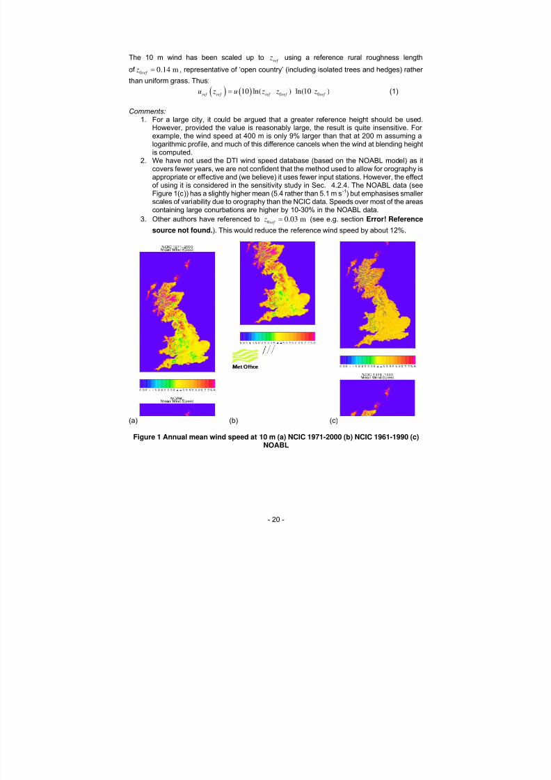
8/6/2019 Best Et Al._small-Scale Wind Energy Technical Report_2008
http://slidepdf.com/reader/full/best-et-alsmall-scale-wind-energy-technical-report2008 152/191
- 20 -
The 10 m wind has been scaled up to using a reference rural roughness length
of , representative of ‘open country’ (including isolated trees and hedges) rather
than uniform grass. Thus:
ref z
0 0.14 mref z =
( ) ( ) 010 ln( ) ln(10 )
ref ref ref ref ref u z u z z z=
0(1)
Comments: 1. For a large city, it could be argued that a greater reference height should be used.
However, provided the value is reasonably large, the result is quite insensitive. For example, the wind speed at 400 m is only 9% larger than that at 200 m assuming alogarithmic profile, and much of this difference cancels when the wind at blending heightis computed.
2. We have not used the DTI wind speed database (based on the NOABL model) as itcovers fewer years, we are not confident that the method used to allow for orography isappropriate or effective and (we believe) it uses fewer input stations. However, the effectof using it is considered in the sensitivity study in Sec. 4.2.4 . The NOABL data (seeFigure 1(c)) has a slightly higher mean (5.4 rather than 5.1 m s -1) but emphasises smaller scales of variability due to orography than the NCIC data. Speeds over most of the areascontaining large conurbations are higher by 10-30% in the NOABL data.
3. Other authors have referenced to 0 0.03 mref z = (see e.g. section Error! Referencesource not found. ). This would reduce the reference wind speed by about 12%.
(a) (b) (c)
Figure 1 Annual mean wind speed at 10 m (a) NCIC 1971-2000 (b) NCIC 1961-1990 (c)NOABL

8/6/2019 Best Et Al._small-Scale Wind Energy Technical Report_2008
http://slidepdf.com/reader/full/best-et-alsmall-scale-wind-energy-technical-report2008 153/191
- 21 -
4.2.2.2 Blending-height wind speedThe grid box-averaged wind speed at the blending height 2 , , is computed using the effective
grid box-averaged roughness length, , and zero-plane displacement height, , thus:bl
0 eff z eff d
( ) ( ) ( )( ) ( )( )0ln - ln -b ref b eff eff ref eff eff u l u z l d z z d z= 0 (2)The grid box-averaged parameters and the grid box blending height are obtained below.
Comments:1. Blending height theory does not usually take into account the zero-plane displacement
height. However, the formulation can be extended quite readily. The main issue is thatthe theory does not give us a method of estimating the grid box averaged zero-planedisplacement height.
4.2.2.3 Grid box-average surface parametersThe grid-box average roughness and displacement height are central to converting the ‘regional’wind speed to something representative of the neighbourhood on the scale of the 1 km grid box.
To derive grid box-average surface parameters we have used a methodology similar to that usedin the Met Office’s UK forecast model. Land use data from the Centre for Ecology and Hydrology(CEH) at 25 m resolution covering 25 categories of surface cover has been aggregated to theproportion of each of 8 surface types in each 1 km square. The two ‘urban’ categories,essentially suburban and dense urban, have been retained but the vegetation categoriessimplified. Note that the CEH data gives us the area of these categories, but tells us nothingmore about them (such as building height). The types and their assumed properties aresummarised in the table below and the proportions of land occupied by the most important typesare shown in Figure 2.
Parameter Surface typeBroad-leavedtrees
Needle-leavedtrees
Grass/Crops
Shrubs Water Soil Sub-urban(Seebelow)
Urban(Seebelow)
Roughnesslength z 0 (m)
0.95 1.075 0.14 0.18 3x10 -4 3x10 -4 0.70 1.60
Canopy Height,h, (m)
19 20 1.4 1.8 0 0 6.00 12.00
Displacementheight, d, (m)
19*2/3 20*2/3 0 0 0 0 3.10 7.00
2
The blending height is the height below which the local wind profile can be treated as being in equilibriumwith the local surface roughness, and above which the area-average profile is in equilibrium with theeffective area-average surface roughness.
8/6/2019 Best Et Al._small-Scale Wind Energy Technical Report_2008
http://slidepdf.com/reader/full/best-et-alsmall-scale-wind-energy-technical-report2008 154/191
- 22 -
Broad-leaved trees Needle-leaved trees Grass
Shrubs Dense urban Suburban
Figure 2 Proportions of different land-use derived from CEH data (supplemented by IGBPover Ireland) for various surface types. Remaining proportions are bare soil and lakes.
Note that the 1990 land cover map has been used (seehttp://www.ceh.ac.uk/sections/seo/lcm1990.html , supplemented by International GeophysicalBiosphere Programme (IGBP) data over Northern Ireland, as this data set has been purchasedby the Met Office. Ideally, the more recent 2000 dataset would be used ( seehttp://www.ceh.ac.uk/sections/seo/lcm2000_home.html ) but this is not readily available to the

8/6/2019 Best Et Al._small-Scale Wind Energy Technical Report_2008
http://slidepdf.com/reader/full/best-et-alsmall-scale-wind-energy-technical-report2008 155/191
- 23 -
Met Office. Consistency checks were performed between UK census population data and land-use data and it is believed that the impact of changes in land-use are very small between thesedatasets.
We characterise the urban surfaces in terms of mean canopy height h, plan area index λ p andfrontal area index λ f . In fact λ p is not required for our approach but is included because somediscussion of it is useful in choosing a value for λ f . We choose the following values:
Assumed values Derived parametersh λ p λ f d/h z 0 /h d z 0
Suburban 6 m 0.4 0.2 0.525 0.117 3.1 m 0.70 mUrban 12 m 0.6 0.3 0.585 0.133 7.0 m 1.6 m
The values for h and λ p have been selected based on our general impressions of UK cities. Moreprecise values would be possible using detailed survey information but this is not readilyavailable in a form which can be applied to the whole of the UK. We note the h values roughly
correspond to the ‘low height’ category and the boundary between the ‘medium height’ and ‘tall’categories in Grimmond and Oke’s (1999) table 6. The urban λ p value corresponds to the ‘highdensity’ category in Grimmond and Oke’s Table 7 and the suburban λ p values falls into theoverlap between their ‘low density’ and ‘medium density’ categories. Values of λ f are generallylower than λ p and, although there is a lot of scatter, λ f = λ p/2 runs roughly though the middle of the data points in figure A1(f) in Grimmond and Oke (1999). In the absence of more detailedsurvey information we have adopted λ f = λ p/2. For estimating d and z 0 we have used theformulae of Raupach (1994, 1995) with κ = 0.4 rather than those of Macdonald et al . (1998) asused by Heath et al. (2007). This is based on the recommendations of Grimmond and Oke(1999), who found that, while Macdonald’s formulae work well in many situations, they tend tounder-predict roughness when λ p > 0.4.
Land-use fractions less than 0.01 have been ignored; otherwise they can, in our approach,dominate the displacement height estimate. The area-averaged displacement height is taken tobe the maximum of that of the non-zero fraction land-use types. The blending height is taken tobe the larger of 10 m or twice the maximum canopy height of any land use with non-zerofraction. In practice, this means that the blending height is somewhere between 10 m and 40 m.The sensitivity to this has not been tested but experience suggests that over this range resultsare quite insensitive. The area-averaged roughness is then taken to be given by:
( )( )( ) ( )( )( ) 20
typesuseLand
20 lnln
−
=
− −=− ∑ iibi
ieff eff b zd lF zd l (3)
where F i denotes the fraction of land use for the ith land use type. The result is shown in Figure3.
Comments:1. The derived urban parameters are important in determining the urban wind speed at a
given height (above ground or roof level). The sensitivity to the assumed urban canopyheight h will be investigated below.
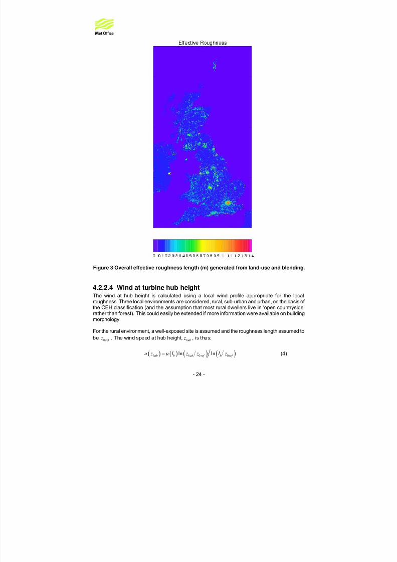
8/6/2019 Best Et Al._small-Scale Wind Energy Technical Report_2008
http://slidepdf.com/reader/full/best-et-alsmall-scale-wind-energy-technical-report2008 156/191
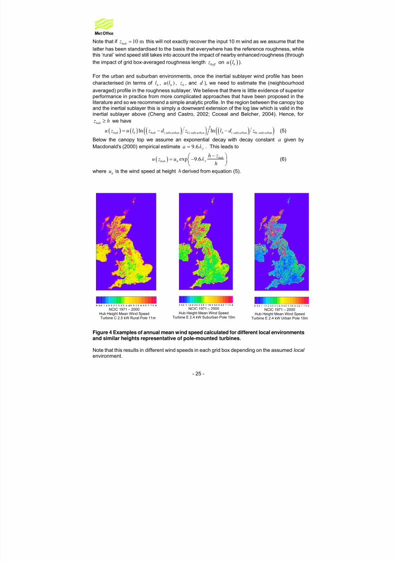
8/6/2019 Best Et Al._small-Scale Wind Energy Technical Report_2008
http://slidepdf.com/reader/full/best-et-alsmall-scale-wind-energy-technical-report2008 157/191
- 25 -
Note that if this will not exactly recover the input 10 m wind as we assume that thelatter has been standardised to the basis that everywhere has the reference roughness, whilethis ‘rural’ wind speed still takes into account the impact of nearby enhanced roughness (throughthe impact of grid box-averaged roughness length on
10 mhub z =
0eff z ( )bu l ).
For the urban and suburban environments, once the inertial sublayer wind profile has beencharacterised (in terms of , , , and d ), we need to estimate the (neighbourhoodaveraged) profile in the roughness sublayer. We believe that there is little evidence of superior performance in practice from more complicated approaches that have been proposed in theliterature and so we recommend a simple analytic profile. In the region between the canopy topand the inertial sublayer this is simply a downward extension of the log law which is valid in theinertial sublayer above (Cheng and Castro, 2002; Coceal and Belcher, 2004). Hence, for
we have
bl )( blu 0 z
hub z ≥ h
( ) ( ) ( )( ) ( )( )( ) 0( ) ( ) 0( )ln lnhub b hub sub urban sub urban b sub urban sub urbanu z u l z d z l d z= − − (5)
Below the canopy top we assume an exponential decay with decay constant given byMacdonald’s (2000) empirical estimate
a f a λ 6.9= . This leads to
( ) exp 9.6 hubhub h f
h zu z u
hλ
− = −
(6)
where is the wind speed at height h derived from equationhu (5) .
Figure 4 Examples of annual mean wind speed calculated for different local environmentsand similar heights representative of pole-mounted turbines.
NCIC 1971 – 2000Hub Height Mean Wind SpeedTurbine C 2.5 kW Rural Pole 11m
NCIC 1971 – 2000Hub Height Mean Wind Speed
Turbine E 2.4 kW Suburban Pole 10m
NCIC 1971 – 2000Hub Height Mean Wind Speed
Turbine E 2.4 kW Urban Pole 10m
Note that this results in different wind speeds in each grid box depending on the assumed local environment.

8/6/2019 Best Et Al._small-Scale Wind Energy Technical Report_2008
http://slidepdf.com/reader/full/best-et-alsmall-scale-wind-energy-technical-report2008 158/191
- 26 -
As examples, the mean wind speeds for pole-mounted turbines at similar heights are shown in
Figure 4 for rural, suburban and urban environments.
Note that these data do not necessarily represent wind speeds that could be measured in reality;if, for example, there were to be an urban area on the top of Cairngorm then the wind speed for a turbine mounted on a 10 m pole would be estimated by the value in the appropriate grid box in
Figure 4 (c), but, since in fact, there is no significant urban area there, the wind-speed shown istoo high (because is too low). However, if a small village were to be built large enough to
have a well defined ‘roughness’, but small enough to have negligible impact on the overallroughness (about 100-200 m across), this would be the wind speed likely at the centre. Therural wind speed is similar (but not identical) to
0eff z
Figure 1(a), the source data, but does show the
impact of urban roughness in the major conurbations. The suburban speed is significantly lower,while the urban speed is very low, reflecting the fact that the height of the wind (10m) is belowthe assumed building height.
Comments:1. Extending the log law into the roughness sub-layer appears to work reasonably well,
but should not be regarded as scientifically justified by inertial sublayer scaling, asthis should not apply so close to the displacement height.
2. The exponential form in eq. 6 is only used when the hub height is below roof level.Given the choice of turbines considered in this study (see section 4.2.3.1 ) this meansthe exponential form is used only for the urban pole-mounted turbines (the roof-mounted turbines and the suburban pole-mounted turbines are all above roof level).This exponential decay emphasises the very substantial reduction in power generation that results from mounting below roof level.
4.2.3 Estimating the Energy Resource
4.2.3.1 Choice of turbinesIn order to estimate the overall energy resource, we have to make decisions about the actualturbines used and their likely mounting. The turbines shown in the following table have beenused as models. In the case of roof-mounted turbines it is assumed that there is a limit on theheight above roof level of the highest part of the device. For a horizontal axis device the highest
point is reached by the tips of the blades, so the hub height is determined from the limiting heightand the rotor diameter. Three maximum heights have been chosen – 3, 4 and 10 m. The 10 mheight is unlikely to be practicable, but has been used to illustrate the benefit to be gained fromuse of a very tall mounting.
Turbine Mounting Hub Height ApplicationTurbine A 15kW Pole 15 m RuralTurbine B 6kW Pole 15 m RuralTurbine C 2.5kW Pole 11 m RuralTurbine D 80W Pole 6 m RuralTurbine E 2.4kW Pole 10 m UrbanTurbine F 1.5kW Roof 1.95 m
2.95 m8.95 m
Urban

8/6/2019 Best Et Al._small-Scale Wind Energy Technical Report_2008
http://slidepdf.com/reader/full/best-et-alsmall-scale-wind-energy-technical-report2008 159/191
- 27 -
Turbine G 1kW Roof 2.125 m3.125 m9.125 m
Urban
The hub heights given for the pole-mounted turbines are height above ground level. The hubheights for the Turbine F and Turbine G are height above roof level and are based on rotor diameters for these devices of 2.1m and 1.75m respectively.
4.2.3.2 Weibull DistributionThe mean wind speed computed above has been converted into a distribution by assuming aWeibull distribution. This is characterised by a scale parameter, A, and a shape parameter, k,thus
( )1
expk k
k u u f u
A A A
− = − (7)
( ) 1 expk
uF u
A
= − − (8)
11u A
k
= Γ +
(9)
Here, ( ) f u is the distribution function, the cumulative distribution function and( )F u u themean speed. Values of obtained by fitting a Weibull distribution to hourly mean speed datavary between 1.5 and 2.1 (based on figures in the European Wind Atlas). Values of
k ( )1 1 1 k Γ +
are tabulated in the European Wind Atlas (Troen and Petersen, 1989):
k A1.6 1.115 u 1.8 1.124 u 2.0 1.128 u
We have assumed 1.8k = . Note gives a Rayleigh distribution.2.0k = Comments:
1. The parameter k determines the relative frequencies of the different wind speedranges and so can have a significant impact on power once combined with the power curves. It determines how long a "tail" exists at high wind speeds which is likely to beespecially important. The sensitivity to k is evaluated below.
4.2.3.3 Mean Power Calculation
Assuming the power curve is defined at 1 m/s intervals and that the wind speed, u , is in m/sthen:
( ) ( ) ( )( )Mean Power 0.5 0.5u
P u F u F u= × + − −∑ (10)
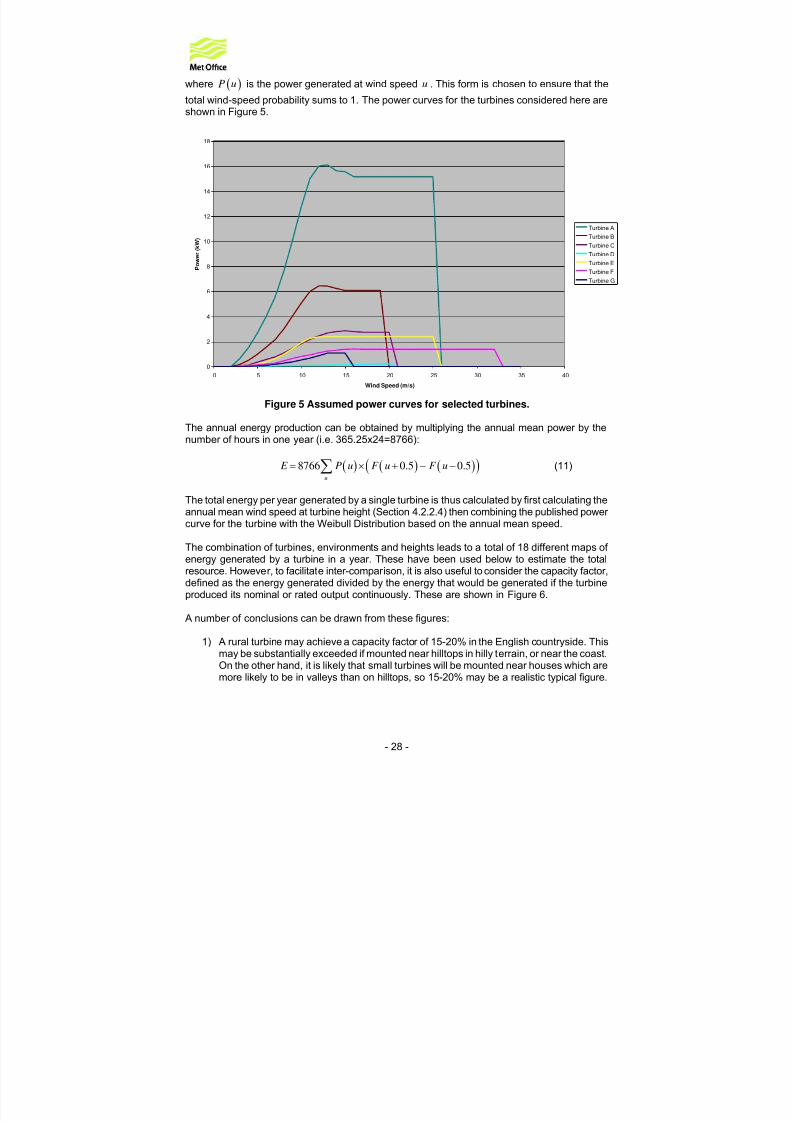
8/6/2019 Best Et Al._small-Scale Wind Energy Technical Report_2008
http://slidepdf.com/reader/full/best-et-alsmall-scale-wind-energy-technical-report2008 160/191
- 28 -
( )P uwhere is the power generated at wind speed u . This form is chosen to ensure that the
total wind-speed probability sums to 1. The power curves for the turbines considered here areshown in Figure 5.
0
2
4
6
8
10
12
14
16
18
0 5 10 15 20 25 30 35 40
Wind Speed (m/s)
P o w e r
( k W )
Turbine A
Turbine B
Turbine C
Turbine D
Turbine E
Turbine F
Turbine G
Figure 5 Assumed power curves for selected turbines.
The annual energy production can be obtained by multiplying the annual mean power by thenumber of hours in one year (i.e. 365.25x24=8766):
( ) ( ) ( )( )8766 0.5 0.5u
E P u F u F u= × + − −∑ (11)
The total energy per year generated by a single turbine is thus calculated by first calculating theannual mean wind speed at turbine height (Section 4.2.2.4 ) then combining the published power curve for the turbine with the Weibull Distribution based on the annual mean speed.
The combination of turbines, environments and heights leads to a total of 18 different maps of energy generated by a turbine in a year. These have been used below to estimate the totalresource. However, to facilitate inter-comparison, it is also useful to consider the capacity factor,defined as the energy generated divided by the energy that would be generated if the turbineproduced its nominal or rated output continuously. These are shown in Figure 6 .
A number of conclusions can be drawn from these figures:
1) A rural turbine may achieve a capacity factor of 15-20% in the English countryside. Thismay be substantially exceeded if mounted near hilltops in hilly terrain, or near the coast.On the other hand, it is likely that small turbines will be mounted near houses which aremore likely to be in valleys than on hilltops, so 15-20% may be a realistic typical figure.
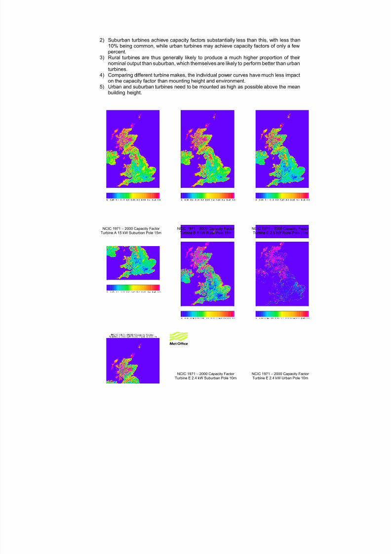
8/6/2019 Best Et Al._small-Scale Wind Energy Technical Report_2008
http://slidepdf.com/reader/full/best-et-alsmall-scale-wind-energy-technical-report2008 161/191
- 29 -
2) Suburban turbines achieve capacity factors substantially less than this, with less than10% being common, while urban turbines may achieve capacity factors of only a fewpercent.
3) Rural turbines are thus generally likely to produce a much higher proportion of their nominal output than suburban, which themselves are likely to perform better than urbanturbines.
4) Comparing different turbine makes, the individual power curves have much less impacton the capacity factor than mounting height and environment.
5) Urban and suburban turbines need to be mounted as high as possible above the meanbuilding height.
NCIC 1971 – 2000 Capacity Factor Turbine A 15 kW Suburban Pole 15m
NCIC 1971 – 2000 Capacity Factor Turbine B 6 kW Rural Pole 15m
NCIC 1971 – 2000 Capacity Factor Turbine C 2.5 kW Rural Pole 11m
NCIC 1971 – 2000 Capacity Factor Turbine D 0.08 kW Rural Pole 6m
NCIC 1971 – 2000 Capacity Factor Turbine E 2.4 kW Suburban Pole 10m
NCIC 1971 – 2000 Capacity Factor Turbine E 2.4 kW Urban Pole 10m
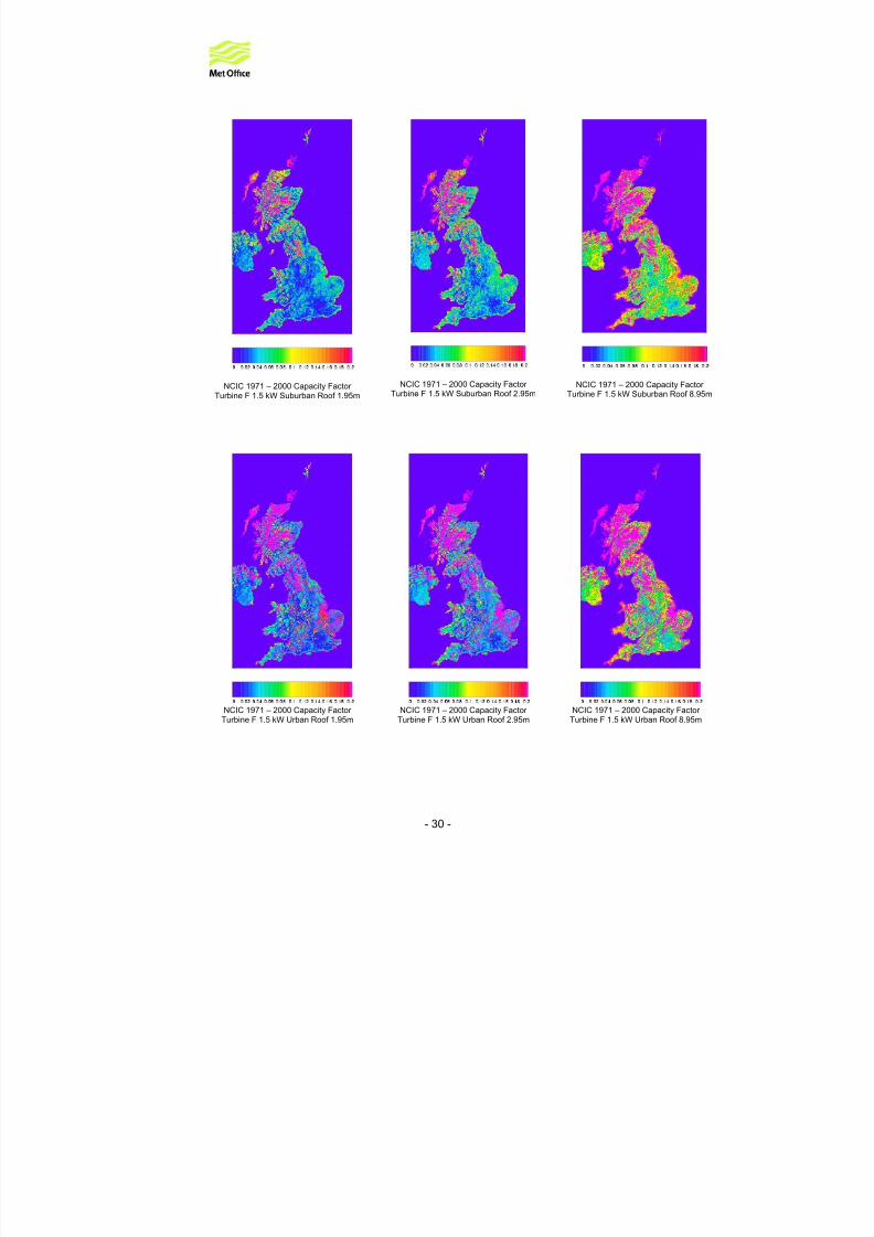
8/6/2019 Best Et Al._small-Scale Wind Energy Technical Report_2008
http://slidepdf.com/reader/full/best-et-alsmall-scale-wind-energy-technical-report2008 162/191
- 30 -
NCIC 1971 – 2000 Capacity Factor Turbine F 1.5 kW Suburban Roof 1.95m
NCIC 1971 – 2000 Capacity Factor Turbine F 1.5 kW Suburban Roof 2.95m
NCIC 1971 – 2000 Capacity Factor Turbine F 1.5 kW Suburban Roof 8.95m
NCIC 1971 – 2000 Capacity Factor Turbine F 1.5 kW Urban Roof 1.95m
NCIC 1971 – 2000 Capacity Factor Turbine F 1.5 kW Urban Roof 2.95m
NCIC 1971 – 2000 Capacity Factor Turbine F 1.5 kW Urban Roof 8.95m
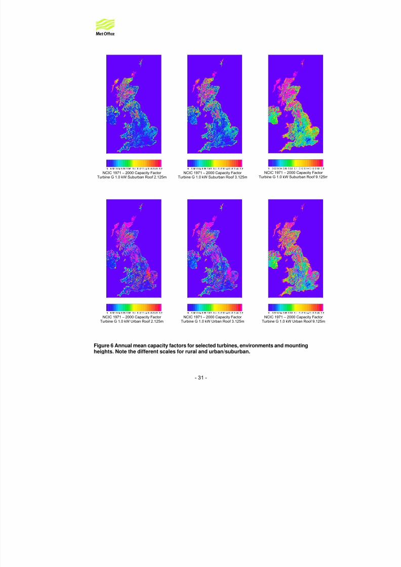
8/6/2019 Best Et Al._small-Scale Wind Energy Technical Report_2008
http://slidepdf.com/reader/full/best-et-alsmall-scale-wind-energy-technical-report2008 163/191
- 31 -
NCIC 1971 – 2000 Capacity Factor Turbine G 1.0 kW Suburban Roof 2.125m
NCIC 1971 – 2000 Capacity Factor Turbine G 1.0 kW Suburban Roof 3.125m
NCIC 1971 – 2000 Capacity Factor Turbine G 1.0 kW Urban Roof 2.125m
NCIC 1971 – 2000 Capacity Factor Turbine G 1.0 kW Urban Roof 3.125m
NCIC 1971 – 2000 Capacity Factor Turbine G 1.0 kW Urban Roof 9.125m
NCIC 1971 – 2000 Capacity Factor Turbine G 1.0 kW Suburban Roof 9.125m
Figure 6 Annual mean capacity factors for selected turbines, environments and mountingheights. Note the different scales for rural and urban/suburban.

8/6/2019 Best Et Al._small-Scale Wind Energy Technical Report_2008
http://slidepdf.com/reader/full/best-et-alsmall-scale-wind-energy-technical-report2008 164/191
- 32 -
4.2.3.4 Total Energy Calculation
We have assumed three different environments for the turbines. ‘Rural’ turbines are assumed to
be used in a rural environment. ‘Urban’ turbines are assumed to be used in either a suburban or urban environment. The maximum energy, M , generated by each turbine type in each 1km cellis given by
h
N M E
n= (12)
This is the energy that would be generated if every household installed each turbine. Here, isthe number of people within each grid box that live in the given environment, is the average
number of people per household (taken to be 2.35, the same), so
N
hn
h N n is the number of households in the grid box.
The value of has been determined for the rural and built-up environments by transferring2001 census data onto the 1km grid. Use has been made of census data for both the ‘Super Output Areas’ of the census (which cover the entire land area of the UK) and urbanareas/settlements (which only cover built-up areas).
N
The census data are initially mapped onto a 100m grid. The boundaries of the urbanareas/settlements are used to determine which 100m grid boxes are classified as ‘built-up’ andwhich are classified as ‘rural’. For the purposes of this analysis only built-up areas with apopulation of 1000 people or more have been used – there are 3019 such areas.
The UK is divided into 9319 Super Output Areas (SOAs). The SOAs are defined such that theyeach contain a similar population, which means that in densely populated parts of the UK the
SOAs are very small. It is therefore possible to determine spatial variations in population densityacross large built-up areas from the SOA census figures. In such regions the population of eachSOA is assumed to be distributed uniformly across the 100m grid boxes that lie within itsboundaries.
In less densely populated regions of the UK the SOAs are much larger and may encompass oneor more smaller settlements. In these regions the population of each settlement is distributeduniformly across the 100m grid boxes within its boundaries. The remaining population in eachSOA (i.e. after subtracting the population of the built-up areas) is distributed uniformly across the100m grid boxes that lie within the SOA but outside the built-up areas.
A few SOAs do not contain any built-up areas and are thus entirely ‘rural’. The population of theSOA is distributed uniformly across all 100m grid boxes within its boundaries.
The final step is to aggregate the 100m population data to 1km resolution to match the grid usedfor the wind speed analysis. The result is a value for the rural population, , and a value for
the built-up area population, , for each 1km grid box. Because of the way in which the
population mapping has been done it is possible for 1km grid boxes around the fringes of built-up areas to contain both a rural population and an urban population.
rural N
upbuilt N −
The rural population is identified as living in the rural environment. We have split the number of people living in built-up areas, , into suburban and urban populations according to the
proportions of suburban and urban land use (and assumed suburban for the small number of
upbuilt N −

8/6/2019 Best Et Al._small-Scale Wind Energy Technical Report_2008
http://slidepdf.com/reader/full/best-et-alsmall-scale-wind-energy-technical-report2008 165/191
- 33 -
cells with no suburban or urban land use). The numbers of households in each categoryobtained by this method are: 2.373 million rural, 4.365 million urban, 18.177 million suburban.
In practice, some cells generate more energy per turbine than others. We have ordered the gridboxes by descending power generated per turbine and plotted three graphs:
1) Total energy, i.e. the cumulative sum of M2) The average capacity factor, given by the cumulative sum of M divided by both the
cumulative sum of households and by the rated energy per year (i.e. the rated power times number of hours per year). This represents a measure of the return in terms of power generated compared with that obtained if the turbine generates at its rated valueall the time.
3) Average cost factor given by 1000 times the inverse total energy. This is a relativemeasure of the cost per unit of energy generated. It needs to be multiplied by actualannual cost to get a unit energy cost. The factor 1000 is used merely to scale the outputto a more easily plotted value (noting that annual costs are likely to be of order £100-1000). Thus, for example, if a 1 kW generator ran constantly (with capacity factor 1) itwould provide 8766 kWh per year. If the running cost was £1000 (obviously rather high!)the cost factor would be 1000/8766=0.114.
Each is plotted against the cumulative sum of households. The plots for each combination of turbine, environment and height are shown in Appendix A .
In practice, not all households will install a turbine. If f is a factor to allow for marketpenetration, energy losses, etc., we may estimate the total energy generated two ways. If noaccount is taken of the return (i.e. a random proportion, f , install turbines) then the total energygenerated is just f times the total energy generated if all households install a turbine (i.e. themaximum value in the first graph). Alternatively, an optimal set of users are that portion f of households closest to the left of the first graph. If we take 0.01 f = , we obtain the following:
Table 1 Annual energy generation from various turbine/mounting choices.
Rating(kW)
Environment Mounting Height(aboveroof for
roofmounted)
MaximumEnergy
Generated(TWh/year)
EnergyGenerated
1% RandomPenetration(TWh/year)
EnergyGenerated
1% OptimalPenetration(TWh/year)
15.000 Rural Pole 15.000 70.73254 0.70733 1.879176.000 Rural Pole 15.000 27.09664 0.27097 0.678022.500 Rural Pole 11.000 8.60518 0.08605 0.266430.080 Rural Pole 6.000 0.30142 0.00301 0.011072.400 Urban Pole 10.000 0.11891 0.00119 0.031482.400 Suburban Pole 10.000 17.15543 0.17155 0.858891.500 Urban Roof 1.950 1.41376 0.01414 0.104241.500 Suburban Roof 1.950 6.36949 0.06369 0.288911.500 Urban Roof 2.950 1.81141 0.01811 0.122691.500 Suburban Roof 2.950 8.3071 0.08307 0.358811.500 Urban Roof 8.950 3.9884 0.03988 0.197371.500 Suburban Roof 8.950 17.8332 0.17833 0.642811.000 Urban Roof 2.125 0.50902 0.00509 0.05953
1.000 Suburban Roof 2.125 2.35314 0.02353 0.169471.000 Urban Roof 3.125 0.70633 0.00706 0.06967

8/6/2019 Best Et Al._small-Scale Wind Energy Technical Report_2008
http://slidepdf.com/reader/full/best-et-alsmall-scale-wind-energy-technical-report2008 166/191
- 34 -
1.000 Suburban Roof 3.125 3.35195 0.03352 0.215841.000 Urban Roof 9.125 1.95827 0.01958 0.103961.000 Suburban Roof 9.125 8.98625 0.08986 0.38461
Note: Each row in the table gives an estimate of the energy that would be generated if 1% of households in the specified environment install the specified turbine at the specified height. Anestimate of the total UK energy resource from a 1% take up can be obtained by taking aweighted average of the four rural values (based on the expected distribution of turbine choices),doing the same for suburban and urban, and then adding the three amounts together. Note alsothat the number of significant figures in the table does not imply accuracy - these have beenretained only to facilitate onward calculations.
The conclusions drawn in Section 4.2.3.3 are supported by the graphs in Appendix A and thenumbers derived in the table above. In addition, we may conclude that:
1) Height above roof level is a critical parameter. For random market penetration changingthe limit on the height of the highest point of the turbine from 3 m to 4 m is estimated toincrease power output by a factor of around 1.3 to 1.4, and by a factor of 3 to 4 if theheight limit is increased to 10m. The increase is less for optimal sites, with factors of 1.2and 2 for height limits of 4m and 10m respectively (compared with a height limit of 3m).
2) The capacity factor plots shown in Appendix A show that some households are better located than others – in the urban and suburban context these are generally in smalltowns and villages so that they benefit from generally stronger local winds, though larger scale geographical variation is also a factor. However, the achievable energy generationper household changes quite slowly once penetration exceeds a few percent.
3) At the 1% market penetration level, rural energy generation can be improved by factorstypically of 2.5-3 by targeting the optimal households. In suburban areas, this factor is
higher, ranging from 4 to 7. However, this primarily reflects the low capacity factor (lessthan 5%) achieved at most locations. Even higher factors can occur in urban areas(reflecting even lower capacity factors).
4) Even though the suburban households outnumber the rural households by roughly 8 to1, the rural resource is potentially larger (at the same level of penetration) becausecapacity factors are larger and pole-mounting enables use of larger turbines.
5) Put simply, the more rural a location, the more potential for energy generation there is;urban dwellers in villages will achieve more return than those in towns, those at theedges of towns will be favoured over those at the centre, and those in small towns will befavoured over those in large towns or cities. For the majority of households, these factorsoutweigh regional (non-urban) differences in wind climatology (see Figure 6 ).

8/6/2019 Best Et Al._small-Scale Wind Energy Technical Report_2008
http://slidepdf.com/reader/full/best-et-alsmall-scale-wind-energy-technical-report2008 167/191

8/6/2019 Best Et Al._small-Scale Wind Energy Technical Report_2008
http://slidepdf.com/reader/full/best-et-alsmall-scale-wind-energy-technical-report2008 168/191
- 36 -
Table 4 Percentage change in total annual energy generated for 1% optimalpenetration ( Table 1 ) by various turbine/mounting choices for changes in input
assumptions (see Table 2 for key).
Turbine Rating(kW)
Environment Mounting Height(aboveroof for
roofmounted)
(m)
NL ZR TB RA
Turbine A 15 Rural Pole 15 -0.9 0.3 -0.1 4.4Turbine B 6 Rural Pole 15 -0.3 0.2 -0.1 6.6Turbine C 2.5 Rural Pole 11 -0.9 0.3 -0.1 5.1Turbine D 0.08 Rural Pole 6 -2.0 0.5 -0.1 1.4Turbine E 2.4 Urban Pole 10 31.3 2.4 -90.1 -10.6Turbine E 2.4 Suburban Pole 10 2.2 0.9 -28.6 -3.9
Turbine F 1.5 Urban Roof 1.95 20.5 0.9 -7.5 -2.8Turbine F 1.5 Suburban Roof 1.95 2.4 1 5.8 -5.9Turbine F 1.5 Urban Roof 2.95 19.3 0.8 -8.6 -2.0Turbine F 1.5 Suburban Roof 2.95 2.3 1 3.3 -4.9Turbine F 1.5 Urban Roof 8.95 14.2 0.5 -8.1 0.8Turbine F 1.5 Suburban Roof 8.95 1.8 0.7 0.5 -1.4Turbine G 1 Urban Roof 2.125 22.1 0.6 -5.3 -2.4Turbine G 1 Suburban Roof 2.125 2.8 1.2 6.2 -8.6Turbine G 1 Urban Roof 3.125 19.5 0.5 -6.0 -1.0Turbine G 1 Suburban Roof 3.125 2.5 1.0 3.2 -6.4Turbine G 1 Urban Roof 9.125 8.9 -0.1 -4.1 4.3
Turbine G 1 Suburban Roof 9.125 1.6 0.5 0.0 1.9 The following conclusions may be drawn from these sensitivity tests:
1) The choice of reference height, ref z , has only minor impact on the results.
2) The building height assumption generally has an impact of less than 10%, and may be of either sign for roof-mounted turbines (tall buildings tending to increase the power insuburban areas, and decrease power in dense urban areas, presumably because of competing factors of increasing overall roughness (and so decreasing wind speed) andlifting the turbine higher in the wind profile. On the other hand, the pole-mountedurban/suburban turbine is extremely sensitive to building height, as an increase inbuilding height moves it closer to roof top in the suburban case (where it is mountedabove roof top height) and further into the urban canopy in the urban case. As a result,the Turbine E results must be regarded as much more uncertain and, in practice,sensitive to the precise local building heights.
3) The Weibull shape parameter also generally has an impact of less than 10% except for the Turbine E and Turbine G with random penetration, where the impact can be closer to20%. This presumably reflects sensitivity to the frequency of wind around their lower cut-in limit (about 4 m s -1) which changes significantly with the shape of the wind-speeddistribution.
4) The choice of annual mean wind speed has the largest impact with random penetration,as much as 73% (although this applies to a turbine generating very little energy).Certainly, 50-60% change is plausible. This reflects the different spatial patterns, as the
overall average wind speed is very comparable. It is clear from Figure 1 that the NOABLdata shows much less variability on large scales but much more on small scales.
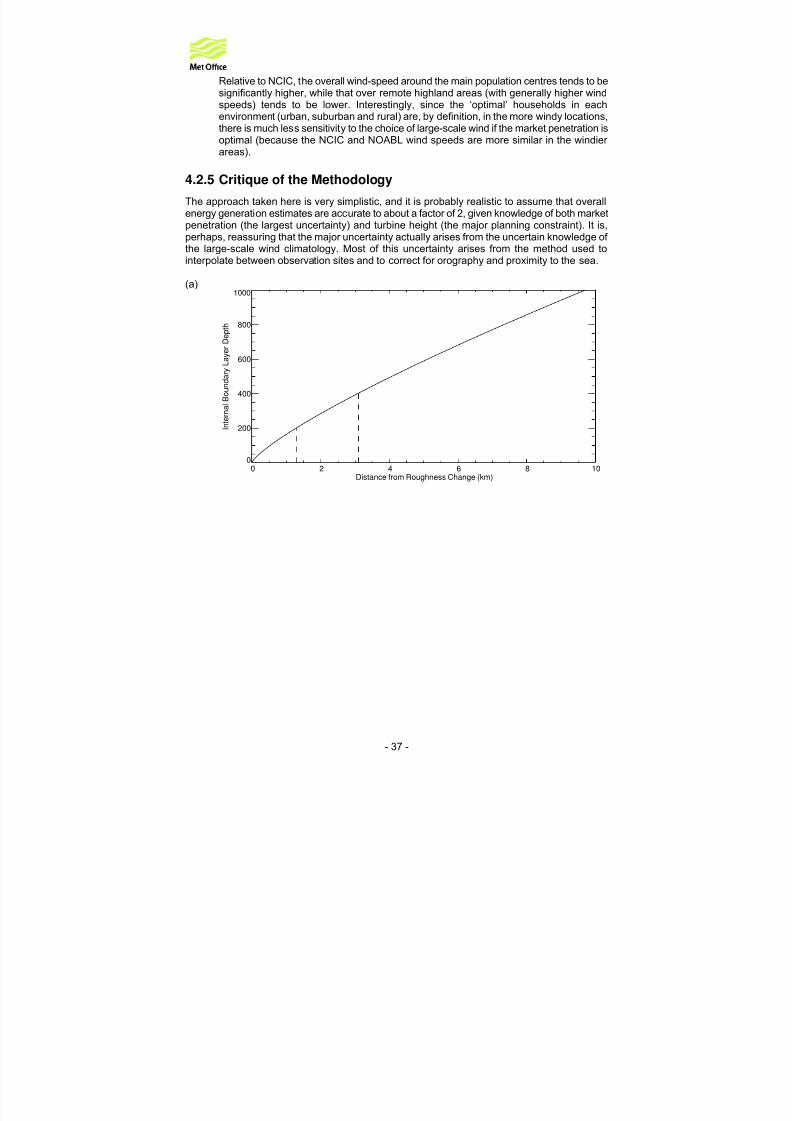
8/6/2019 Best Et Al._small-Scale Wind Energy Technical Report_2008
http://slidepdf.com/reader/full/best-et-alsmall-scale-wind-energy-technical-report2008 169/191

8/6/2019 Best Et Al._small-Scale Wind Energy Technical Report_2008
http://slidepdf.com/reader/full/best-et-alsmall-scale-wind-energy-technical-report2008 170/191
- 38 -
(b)8
Figure 7 Idealised profiles of (a) internal boundary-layer height and (b) wind speed 10m above the displacement height using the Elliot Internal Boundary Layer formulation
for a 10 m s -1 geostrophic wind. In (b) the uniform wind speed assuming RossbySimilarity Theory (RST) over the rural and urban areas is shown along with the wind
speed derived using reference heights of 200 m and 400 m.
A second major deficiency is neglect of edge or directional effects. Buildings on the ‘upstream’edge of a city will experience stronger winds than implied by the ‘equilibrium’ approach adopted.This is allowed for to a small extent by using a relatively low reference height. This is illustratedin Figure 7 . Note that even this picture is idealised – real rural/urban transitions are complicatedby stability effects. This figure shows that the method used is likely to substantially under-estimate the wind over the first 500 m or so from the edge of the city, and slightly over-estimate(by, perhaps 0.5 m s -1) elsewhere. Clearly, the overall error depends on the size of the city. Witha uniform distribution of wind direction, buildings in the transition zone will experience enhancedspeed half the time (though the depth of the zone at a particular part of the city edge will varywith wind direction).
It is possible to roughly estimate the proportion of buildings that could be affected by thisboundary zone. Using the land-use data we can estimate the area of contiguous regions of urban area (defined as urban+suburban fraction greater than some threshold). If we assume thatthese contiguous regions are circular and the depth of the boundary region is 0.5 km, with a
threshold of 50% urban cover we estimate that about 6% of buildings are in the boundary region(and so, allowing for variation of wind direction, experience more rural wind-speeds about 32 %of the time). This effect could therefore be very crudely allowed for by re-allocating about 2% of the suburban population to rural, an increase of rural households by about 15%. This is wellwithin the overall uncertainty of the method.
The other area of obvious weakness is the crude assumptions made concerning morphology of buildings in urban areas. Obtaining detailed information concerning building heights and areas isdifficult and, generally, the data are proprietary and expensive. The above sensitivity studysuggests the results are not extremely sensitive for roof-mounted turbines (mounted above roof level), but much more so for fixed-height pole-mounted turbines. This sensitivity could beexplored further using, for example, distributions of parameters rather than constant values, and,perhaps, using census data on detached, semi-detached etc. houses, but assumptions wouldstill be required about morphology and distribution.
0 2 4 6 8 10
Distance from Roughness Change (km)
2
4
Rural RST Equilibrium
1 0 m
w i n d s p e e
d ( m / s )
6
Elliot IBL
Urban RST Equilibrium
zref=200 m
zref=400 m

8/6/2019 Best Et Al._small-Scale Wind Energy Technical Report_2008
http://slidepdf.com/reader/full/best-et-alsmall-scale-wind-energy-technical-report2008 171/191
- 39 -
Related to this is the assumption of a uniform number of people per household. In practice, thisvaries with location and housing type, and the influence of this could be taken into account. It isdifficult, however, to separate this from more socio-economic studies of the likely uptake of turbines. In practice, it is unlikely that uptake will be random – presumably turbines are morelikely to be installed by those with more disposable income. Fortuitously, this may bias uptaketowards the more optimal locations, but estimating the extent of this bias is beyond the scope of this study.
4.2.6 Outline of Possible Improvements
The analysis methodology described in the preceding sections has been constrained in part bythe specific aims and scope of the current project. There are various aspects of the approachthat could potentially be improved and these are discussed below:
a) Large-scale climatology
Given the large sensitivity of the overall UK energy resource to the mean large scale windspeed, alternative approaches to determining this should be investigated. A convenient andcomprehensive data source is the Met Office archive of operational NWP analyses andforecasts. Winds from relatively fine resolution NWP models (with horizontal grid of 12km) areavailable from the last 10 years. Data from a finer resolution 4km model for a shorter recentperiod of15 months can also be used. These have the advantage that model winds are sampledat a finer scale than the conventional wind observations, which form the basic input to both theNCIC and NOABL data. The NWP models carry forward the observational data from previoustimes and adjust winds dynamically to the finer scales. The NWP winds can be processed toform annual mean wind speed estimates, as for the NCIC and NOABL data used above,combined with a Weibull distribution. Rather than assumed parameters for the distribution, thesecould be fitted by also calculating the mean cubed wind. However there is scope for moreaspects to be investigated. A frequency of wind speeds by directional sectors (wind rose) couldbe employed, using the analyses (4 per day) and short period hourly forecasts. This may beapplied either directly or by fitting to intermediate Weibull distributions in each sector. Thesensitivity of power generation to diurnal and seasonal variations in wind speeds could also beinvestigated with NWP data.
Whilst NWP data provides greater opportunity to look at these directional, seasonal and other influences, the processing is necessarily more extensive and costly.
b) Modelling of Orography
The NCIC and NOABL data both take into account orography at fine scale, though using verydifferent methods and obtaining very different results. It is likely that both suffer from errors atintermediate scales (10-50 km) which are likely to be affected by non-linear processes andstability effects. These scales should be better handled by the NWP data (especially at 4 kmresolution), but the finer scales are not treated. Linear models could be used to downscale NWPdata to fine-scale orography, using a linear flow model such as MS3DJH or the potential flow
part of such a model for gridded data, or using WAsP where individual site studies are required.

8/6/2019 Best Et Al._small-Scale Wind Energy Technical Report_2008
http://slidepdf.com/reader/full/best-et-alsmall-scale-wind-energy-technical-report2008 172/191
- 40 -
c) Edge Effects
In the present analysis the reference height , z ref , has been fixed at a value of 200m. In Section4.2.5 it was shown that this has the effect of underestimating the wind speeds in the fringes of urban areas and overestimating the wind in areas further towards the centre. Although thesensitivity tests indicate that changing this value does not have a large impact, one option wouldbe to allow the reference height value to vary across the UK, in accordance with the scale of heterogeneity in the surface roughness. A finer classification of urban area may be achievable,including ‘distance from edge of town’ to enable a different reference height to be used close tothe edge of towns. If directionally dependent wind data are used, the direction to the edge couldalso be employed to enable a reference height based on the internal boundary layer depth to beused. Such an approach may need to be fine-tuned by comparison with more detailed models(for a small selection of conditions). A particular issue is the precise definition of town edge. Inmany cases there is a clear demarcation, but in others the rate of change of effective surfaceroughness may be quite slow and an accurate approach may be difficult to define.
Such an approach may not be justified for estimation of overall resource because, as discussedabout, other factors dominate uncertainty. However, in selecting locations for individual turbines(or advising an installer on likely output) these effects may be very important, as the optimallocations for urban installation will lie close to the edge of towns.
d) Directional Dependencies / Fetch Effects
There is no allowance for wind direction in the current analysis. Clearly the wind does not blowfrom all directions with equal frequency, nor, in general, is the upwind roughness length thesame in all directions. Use of directionally-dependent data (such as mean wind speed and
Weibull parameter for different wind sectors, where a wind sector might cover 30 °) wouldfacilitate a directionally dependent interaction with orography and a more accurate treatment of edge effects as discussed above.
e) Blending Height and related parameters
Further work is required to test the sensitivity of the results to the algorithm used to determinethe blending height and parameters related to it. Blending heights are theoretically well definedwhere the characteristic length scale for variability of surface is well defined. This is very difficultto establish in practice, but better classification of surface parameters and analysis of scales of variability (e.g. through wavelet analysis of roughness) might enable a more scientifically
rigorous blending height to be defined.
In addition, the effective displacement height is poorly defined and there is very little literature onthe subject. Alternative approaches should be considered, based on alternative weightings of theindividual surface type displacement height, and sensitivity tests conducted.
f) Stability Effects
The calculations currently assume that the stability of the atmosphere is neutral. NWP data doinclude a measure of surface stability, and this could be incorporated by using Monin Obukhov Similarity Theory to replace the logarithmic profiles used with stability-dependent profiles.

8/6/2019 Best Et Al._small-Scale Wind Energy Technical Report_2008
http://slidepdf.com/reader/full/best-et-alsmall-scale-wind-energy-technical-report2008 173/191
- 41 -
g) Building Morphology
The values of mean building height, , plan area density,h pλ , and frontal area density, f
λ , have
been assigned fixed values for the urban and suburban environments. Consequently the
roughness length, , and displacement height, , also have fixed values. In reality thesevalues would vary from one urban area to another and between different neighbourhoods withina single urban area. This is likely to be more important in estimating the energy from a singleturbine than in estimating the overall UK resource.
0 z d
A possible alternative approach would be to use housing stock information to estimate spatially-varying values for the building height and densities. Potentially suitable data can be obtainedfrom census information. This includes the numbers of detached, semi-detached and terracedproperties, and the number of flats or apartments, in each urban area/settlement. However thiswould have to be supplemented by information or assumptions on the non-residential buildings.
h) Market Size
To calculate the total UK wind energy resource it is necessary to estimate the size of the marketfor small-scale wind turbines. This is currently done by calculating the number of households ineach part of the country by scaling the population by the average number of people per household (assumed to be 2.35). A potential improvement would be to use the actual number of households in each area, as recorded in the census data.
i) Weibull Shape Parameter
The frequency distribution of wind speed is modelled using a Weibull distribution with a fixed
shape parameter of 1.8. The sensitivity tests show that changing this value does have an impacton the estimated resource, particularly if the take-up of turbines is not optimal.
Given that the impact is non-linear, it may be worth examining how the shape parameter variesfrom place to place across the UK. This could be done from existing archives of hourly meanwind speed data.
j) Short-duration Fluctuations
Variations in wind speed and direction over short time-scales (seconds to minutes) are notaddressed in the current analysis procedure. Small turbines can respond fairly rapidly to
changes in wind speed. Given the non-linear relationship between wind power and wind speed,ignoring these fluctuations (by using hourly mean speeds) may lead to an underestimate of theavailable wind power. Conversely, variations in speed around the cut-in and cut-out speedscould lead to a reduction in energy generation due to the turbine becoming disconnected fromthe power distribution network. Fluctuations in wind direction will always tend to reduce theturbine efficiency, so ignoring these could result in an overestimate of the energy resource.
To determine whether these are significant effects, an assessment could be carried out of anydifferences that may be observed between the frequency distributions of hourly means and 1-minute means obtained from surface anemometer data. If higher frequency data is needed astochastic model of the sub 1 minute fluctuations could be used to supplement the data.However for accurate results (and to take any account for the reduction in turbine efficiency dueto wind direction fluctuations) it would be necessary to combine this with a model for the turbineresponse.

8/6/2019 Best Et Al._small-Scale Wind Energy Technical Report_2008
http://slidepdf.com/reader/full/best-et-alsmall-scale-wind-energy-technical-report2008 174/191
- 42 -
k) Local Effects / Micro-siting
In assessing the UK wind energy resource no attempt has been made to model the impacts of either nearby obstacles or the topography of the immediate area (e.g. trees, hedges, banks,surrounding houses), nor has any account been taken of the effect on roof-mounted turbines of the building itself.
It would not be practical to include such effects in an assessment of the total UK resource,especially as the precise locations where turbines will be installed are not known. However, if anestimate is required for a specific location then it should be possible to extend the basicapproach to give a more site-specific result. Examples of how this could be achieved include:
- The values of mean building height and plan and frontal area densities could be obtainedby inspection of the neighbourhood surrounding the target site or from aerialphotographs.
- For a rural location the roughness length could be estimated from an inspection of thesurrounding area.
- A site inspection could be used to identify sectors where there are obstacles that couldhave a significant impact on the local wind flow. The assessment would need to consider the properties of the surrounding obstacles (tall, thin buildings have a different impact tolow, wide buildings) and the conclusions would be dependent on whether the turbine is tobe located above or below the mean building height.
- For roof-mounted turbines it would also be necessary to consider the height above roof level. The impact will differ for flat-roofed and pitched-roofed buildings, and will dependon the position of the turbine on the roof relative to prevailing wind direction.
The effects of local building geometry are complicated and difficult to predict – consequently it isnot anticipated that definitive ‘correction factors’ could be determined that would have generalapplicability. Instead the assessment process described above would identify energy that was ‘atrisk’. To find out how much energy is actually lost in practice would require a more detailed siteassessment, perhaps including wind measurements at the proposed turbine location.
Note that to allow properly for local obstacles and building geometry it is necessary to retaininformation on the distribution of wind directions, rather than simply working in terms of windspeeds.
l) Calibration and Verification
Ideally the estimates produced in this study would be compared with observations in order toassess objectively their accuracy and/or calibrate the output. Given the number of turbinesinstalled in the UK is still quite small, verification of the total UK wind energy resource is clearlyimpractical. However it may be possible to test some aspects of the calculations, for example:
- Roughness lengths and displacement heights for some limited urban areas could becomputed using real building data and compared with the values obtained usingassumed values for mean building height and density. There are a number of potentialsources of suitable building data, including block models and digital surface models fromGetmapping.com and the Virtual London project run by University College London.
- The predicted wind at blending height could be compared with observations from roof-mounted anemometers in urban areas (e.g. London Weather Centre).

8/6/2019 Best Et Al._small-Scale Wind Energy Technical Report_2008
http://slidepdf.com/reader/full/best-et-alsmall-scale-wind-energy-technical-report2008 175/191

8/6/2019 Best Et Al._small-Scale Wind Energy Technical Report_2008
http://slidepdf.com/reader/full/best-et-alsmall-scale-wind-energy-technical-report2008 176/191
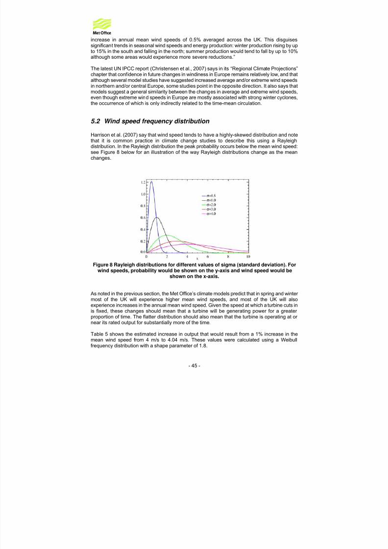
8/6/2019 Best Et Al._small-Scale Wind Energy Technical Report_2008
http://slidepdf.com/reader/full/best-et-alsmall-scale-wind-energy-technical-report2008 177/191
- 45 -
increase in annual mean wind speeds of 0.5% averaged across the UK. This disguisessignificant trends in seasonal wind speeds and energy production: winter production rising by upto 15% in the south and falling in the north; summer production would tend to fall by up to 10%although some areas would experience more severe reductions.”
The latest UN IPCC report (Christensen et al., 2007) says in its “Regional Climate Projections”chapter that confidence in future changes in windiness in Europe remains relatively low, and thatalthough several model studies have suggested increased average and/or extreme wind speedsin northern and/or central Europe, some studies point in the opposite direction. It also says thatmodels suggest a general similarity between the changes in average and extreme wind speeds,even though extreme wind speeds in Europe are mostly associated with strong winter cyclones,the occurrence of which is only indirectly related to the time-mean circulation.
5.2 Wind speed frequency distribution
Harrison et al. (2007) say that wind speed tends to have a highly-skewed distribution and notethat it is common practice in climate change studies to describe this using a Rayleighdistribution. In the Rayleigh distribution the peak probability occurs below the mean wind speed:see Figure 8 below for an illustration of the way Rayleigh distributions change as the meanchanges.
Figure 8 Rayleigh distributions for different values of sigma (standard deviation). For
wind speeds, probability would be shown on the y-axis and wind speed would beshown on the x-axis.
As noted in the previous section, the Met Office’s climate models predict that in spring and winter most of the UK will experience higher mean wind speeds, and most of the UK will alsoexperience increases in the annual mean wind speed. Given the speed at which a turbine cuts inis fixed, these changes should mean that a turbine will be generating power for a greater proportion of time. The flatter distribution should also mean that the turbine is operating at or near its rated output for substantially more of the time.
Table 5 shows the estimated increase in output that would result from a 1% increase in themean wind speed from 4 m/s to 4.04 m/s. These values were calculated using a Weibullfrequency distribution with a shape parameter of 1.8.

8/6/2019 Best Et Al._small-Scale Wind Energy Technical Report_2008
http://slidepdf.com/reader/full/best-et-alsmall-scale-wind-energy-technical-report2008 178/191
- 46 -
Table 5 Percentage Increase in Energy Output for a 1% Increase in the Mean WindSpeed
Turbine Increase in Output (%)Turbine A 15kW 2.3Turbine B 6kW 2.4Turbine C 2.5 kW 2.6Turbine D 80W 2.3Turbine E 2.4kW 3.0Turbine F 1.5kW 2.6Turbine G 1kW 3.4
5.3 Wind direction distribution
The UKCIP02 report gives very little information on possible changes to the wind directiondistribution due to climate change, and the IPCC 2007 report says nothing about possiblechanges to wind directions over the UK or even northern Europe. The UKCIP02 report only givesinformation about possible wind direction changes in the “uncertainties and wider issues”chapter, instead of the main chapters on predicted climate changes. It says that in winter for the2080s, the RCM used in the UKCIP02 report simulates small increases in westerly winds in thesouth, and reduced south-westerlies in the north. It also says that in summer in the 2080s theRCM shows a weak increase in north-westerly flow over Scotland and a weakening of thesummer south-westerly flow over southern England. The report makes it clear that there is lowconfidence in the modelled changes in wind direction, as the generation of the Met Office RCMprevious to the one used in the UKCIP02 report predicted quite different changes in winddirection in all seasons, except for the changes predicted over Scotland in summer.
5.4 Extremes
The UKCIP02 report provides some information on changes to extreme winds e.g. the change inthe daily mean wind speed that is exceeded on average once every N years (also referred to asthe N-year return period value). These are given for future climate scenarios from the 2020s tothe 2080s, and for return periods from 2 to 20 years. The changes in return periods are lessreliable as the return period increases, so the UKCIP02 report concentrates on the changes in 2-year return period (RP) events. It says that by the 2080s, the 2-year RP daily mean wind speedincreases in most parts of the UK in winter, especially in the south of the UK, where it ispredicted to increase by between 4% and 6% (for the high scenario) in many parts. In summer by the 2080s, the 2-year RP daily mean wind speed is predicted to decrease by between 2%and 6% in most parts of the UK in the high scenario, although northern Scotland and the southeast of England are predicted to see little change or slight increases of less than 4%. For theyear as a whole the changes in the 2-year RP daily mean wind speed by the 2080s are predictedto be quite small over most of the UK, even in the high scenario, although in that case someparts of northern England and the far south of England are predicted to see increases of between 4% and 6%. The changes for other scenarios and for the 2050s and 2020s are similar,but of smaller magnitude. It says that the changes in seasonal-average and extreme windspeeds seem to be partly driven in the climate model by a southward movement across the UKof the average winter depression tracks. However, it also cautions that “climate models remainrather poor at simulating small-scale and high intensity wind speeds..., and relatively lowconfidence should be attached to these results.”

8/6/2019 Best Et Al._small-Scale Wind Energy Technical Report_2008
http://slidepdf.com/reader/full/best-et-alsmall-scale-wind-energy-technical-report2008 179/191
- 47 -
Alexander, Tett & Jonsson (2005) examined changes in severe storms (defined as 3-hourlypressure changes exceeding an extreme magnitude) over the UK over the past several decades.They found that the UK regions have tended towards larger magnitude events in recentdecades, particularly in the more southerly regions, and that there has been a significantincrease in the number of severe storms over the UK as a whole since the 1950s providing someevidence for a shift in the North Atlantic storm track.
5.5 Summary of relevant on-going research
A new UKCIP report (UKCIP08) is due for release in the second half of 2008. Like the previousreport, it is again based on data from the Met Office’s RCM. The most important difference willbe that it will use an ensemble of simulations of future global climate, created by varying certainmodel parameters within physically realistic ranges. The results of each model version will beweighted according to how well it represents the current climate and its recent evolution, and as
a result probabilistic climate projections will be produced for the UK for each of three futurescenarios of greenhouse gas emissions (Low, Medium and High). These should better support arisk-based assessment of impacts and adaptations associated with a changing climate.
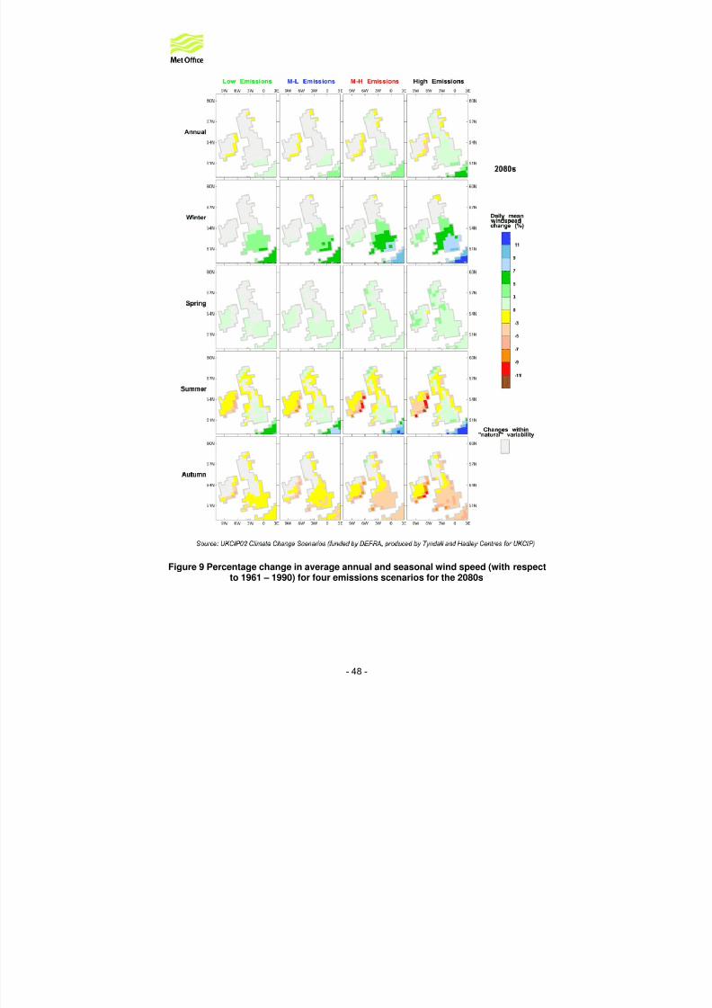
8/6/2019 Best Et Al._small-Scale Wind Energy Technical Report_2008
http://slidepdf.com/reader/full/best-et-alsmall-scale-wind-energy-technical-report2008 180/191
- 48 -
Figure 9 Percentage change in average annual and seasonal wind speed (with respectto 1961 – 1990) for four emissions scenarios for the 2080s

8/6/2019 Best Et Al._small-Scale Wind Energy Technical Report_2008
http://slidepdf.com/reader/full/best-et-alsmall-scale-wind-energy-technical-report2008 181/191
- 49 -
6 Summary
This second phase of the project has examined how the total UK wind energy resource from
small-scale generation may be estimated. A generic approach has been identified in which aseries of correction factors are applied to a large-scale reference wind climatology. Thesecorrection factors modify the reference climatology for the effects of local orography, surfaceroughness and building geometry.
A number of options for generating the reference climatology and the correction factors havebeen evaluated. It is not possible to give a definitive recommendation for the best methods touse without further investigation, especially as the optimal approach will depend on the availableresources, timescales and desired accuracy.
For the purposes of this study a simplified method has been used to generate estimates of UKwind energy resource given various assumptions about turbine characteristics, mounting heightand market penetration. More sophisticated approaches are possible. However the approachadopted here does, we believe, provide a reasonable balance between the need to produce anestimate quickly and the accuracy of the results. The sensitivity of the results to variousparameters and assumptions has been tested.
The approach can be summarised as follows:
- The chosen reference climatology is a 1km grid of the mean wind speed at 10m aboveopen, level terrain, obtained by geostatistical interpolation of surface observations.
- The reference wind speed is transformed up to a reference height of 200m above groundlevel using a roughness length representative of ‘open country’.
- The wind speed at 200m is transformed down to an intermediate blending height usingan area-averaged surface roughness length
- The wind speed at blending height is transformed down to turbine hub height using aroughness length appropriate to the local environment. Three environments relevant tosmall-scale wind turbines are considered – urban, suburban and rural.
- The mean wind speed at hub height is used to define a wind speed frequency distributionusing a Weibull distribution with a fixed shaped parameter of 1.8.
- The wind speed frequency distribution is combined with a turbine power curve to obtainan estimate of the annual energy production from a single turbine. Calculations havebeen done for seven different turbine models, including two roof-mounted systems.
- Grids of ‘energy per turbine’ have been combined with grids of population data. The
results have been accumulated to obtain estimates of the total energy, average capacityfactor and average cost factor for the UK for each turbine system. Figures have beencalculated assuming a market penetration of 1%.
In this study we have chosen to use the NCIC wind speed dataset as our reference climatologyrather than the long-established NOABL dataset. The two datasets may be compared, asfollows:
- Both datasets describe the effects of orography- Neither dataset allows for variations in surface roughness – the wind speed values
represent open, level terrain in a rural environment- NOABL is a 10-year climatology based on 56 stations, whereas the NCIC dataset is a
30-year climatology based on approximately 220 stations

8/6/2019 Best Et Al._small-Scale Wind Energy Technical Report_2008
http://slidepdf.com/reader/full/best-et-alsmall-scale-wind-energy-technical-report2008 182/191
- 50 -
- NOABL was constructed from over-lapping 100x100km tiles, scaled to produce a near-seamless map. The NCIC dataset was generated by fitting a single wind speed modelacross the entire area of the UK.
- In NOABL most of the spatial variation comes from the mass consistent model (becauseeach tile typically contained only one or two observation sites). In the NCIC dataset thespatial variations are inferred empirically from the observations (through a regressionrelationship with terrain elevation, terrain shape etc).
Ultimately wind speed is a complex quantity to interpolate and neither dataset can be expectedto model the true wind climatology perfectly. The comparison of NOABL with long-term stationaverages suggests that this dataset underestimates slightly for higher wind speed sites andoverestimates for lower wind speed ones. On balance, the larger amount of data used, thegreater homogeneity of the analysis method and the empirical approach to characterising thespatial variations were considered sufficient reasons to prefer the NCIC dataset as the basis for the calculations in this report.
The main findings of this study are:
1) Rural turbines are generally likely to produce a much higher proportion of their nominaloutput than suburban, which themselves are likely to perform better than urban turbines.A rural turbine may achieve a capacity factor of 15-20% in the English countryside. Thismay be substantially exceeded if mounted near hilltops in hilly terrain, or near the coast.Suburban turbines achieve capacity factors substantially less than this, with less than10% being common, while urban turbines may achieve capacity factors of only a fewpercent.
2) Comparing different turbine makes, the individual power curves have much less impact
on capacity factors than mounting height and environment.3) Some households are better located than others – in the urban and suburban context
these are generally in small towns and villages so that they benefit from generallystronger local winds, though larger scale geographical variation is also a factor.However, the achievable energy generation per household changes quite slowly oncepenetration exceeds a few percent.
4) Urban turbines need to be mounted as high as possible above the mean building height.Height above roof level is a critical parameter – for random market penetration changingthe limit on the height of the highest point of the turbine from 3 m to 4 m is estimated toincrease power output by 30 to 40%, and increasing the limit to 10 m can increase power
by a factor of 3 to 4 compared with a 3 m height limit (the increases are less for optimalsites). Turbines mounted below roof height, as may be the case for pole-mountedturbines in dense urban areas, on average experience very low wind speeds and sogenerate little power.
5) At the 1% market penetration level, rural energy generation can be improved by factorstypically of 2.5-3 by targeting the optimal households. In suburban areas, this factor ishigher, ranging from 4 to 7. However, this primarily reflects the low capacity factor (lessthan 5%) achieved at most locations. Even higher factors can occur in urban areas(reflecting even lower capacity factors).
6) Even though the suburban households outnumber the rural households by roughly 8 to1, the rural resource is potentially larger (at the same level of penetration) becausecapacity factors are larger and pole-mounting enables use of larger turbines.

8/6/2019 Best Et Al._small-Scale Wind Energy Technical Report_2008
http://slidepdf.com/reader/full/best-et-alsmall-scale-wind-energy-technical-report2008 183/191
- 51 -
7) Put simply, the more rural a location, the more potential for energy generation there is;urban dwellers in villages will achieve more return than those in towns, those at theedges of towns will be favoured over those at the centre, and those in small towns will befavoured over those in large towns or cities. For the majority of households, these factorsoutweigh regional (non-urban) differences in wind climatology.
8) The uncertainty in overall estimates of mean generation arising from meteorologicalassumptions (as opposed to assumption about market penetration and mounting height)is about a factor of two. The dominant source of this uncertainty is the choice of windclimatology used in the computation (including methods used to interpolate and allow for orography). Here we have used the Met Office 1971-2000 climatology generated bygeostatistical interpolation of surface data. It is clear from Figure 1 that the NOABL datashows much less variability on large scales but much more on small scales. The overallwind-speed around the main population centres tends to be significantly higher, whilethat over remote, highland areas, tends to be lower. The choice of annual mean windspeed has the largest impact with random penetration. Interestingly, since the ‘optimal’households in each environment (urban, suburban and rural) are, by definition, in themore windy locations, there is much less sensitivity to choice of large-scale wind if themarket penetration is optimal (because the NCIC and NOABL wind speeds are moresimilar in the windier areas).
A number of potential improvements to the analysis method have been identified. Of these theones most likely to deliver significant benefit in terms of improved accuracy are:
1) Use of a directionally dependent wind climatology, preferably taking into account spatial
and directional variation in the shape of the wind speed distribution (as well as in themean wind speed).2) Incorporation of edge and fetch effects and the influence of small scale orography (using
directionally-dependent data).3) Incorporation of better knowledge of building characteristics (height, area etc.).

8/6/2019 Best Et Al._small-Scale Wind Energy Technical Report_2008
http://slidepdf.com/reader/full/best-et-alsmall-scale-wind-energy-technical-report2008 184/191
- 52 -
7 Conclusions
In the Introduction to Part 1: A Review of Existing Knowledge we began by setting out the
following two key questions:
a) What is the total potential wind energy resource in the UK from small-scale turbines?
b) What is the potential wind energy resource at any given location?
In this report we have described a methodology for estimating the mean wind speed at turbinehub height for a number of different environments (urban, suburban and rural). We have usedthis methodology to generate grids of wind speed data for the UK and we have demonstratedhow these data can be combined with turbine power curves and population data to obtain anestimate of the total small-scale wind energy resource.
The main conclusions from this analysis are:
1) The urban environment has a dramatic impact on wind speed and wind power generationcapacity.
2) This impact varies considerably with height relative to roof-top. The sheltering effect dueto surrounding buildings means that turbines mounted below rooftop are unlikely togenerate, on average, capacity factors of more than a few percent. Significantimprovements can be gained by mounting above rooftop, but heights several metresabove rooftop are likely to be required.
3) Rural turbines typically have higher capacity factors, with 15%-20% being typical andmore being achievable at some locations.
4) To maximise return from investment and carbon savings, turbines should be installed inlocations as rural as feasible, i.e. hill-top sites rather than valleys, open countrysiderather than forested, isolated buildings rather than villages rather than towns, edges(within a few 100 m) of towns rather than in the centre.
As well as estimating the UK resource, the approach described in this report could, in principle,be used to compute an estimate of the resource at an individual location. Although suchestimates would give a useful guide to the wind energy potential at the neighbourhood scale,they would not allow for detailed local effects such as sheltering by individual buildings or trees,very local variations in surface roughness or small-scale terrain effects. The importance of thesefactors in determining turbine yields was highlighted in the siting guidelines set out in section 7 of
Part 1: A Review of Existing Knowledge.We recommend that if the techniques described here are to be used to provide individualhouseholders with an evaluation of their site then any energy estimates must be accompaniedby clear guidance on the limitations of the methodology and the importance of good micro-sitingfor optimum turbine performance.
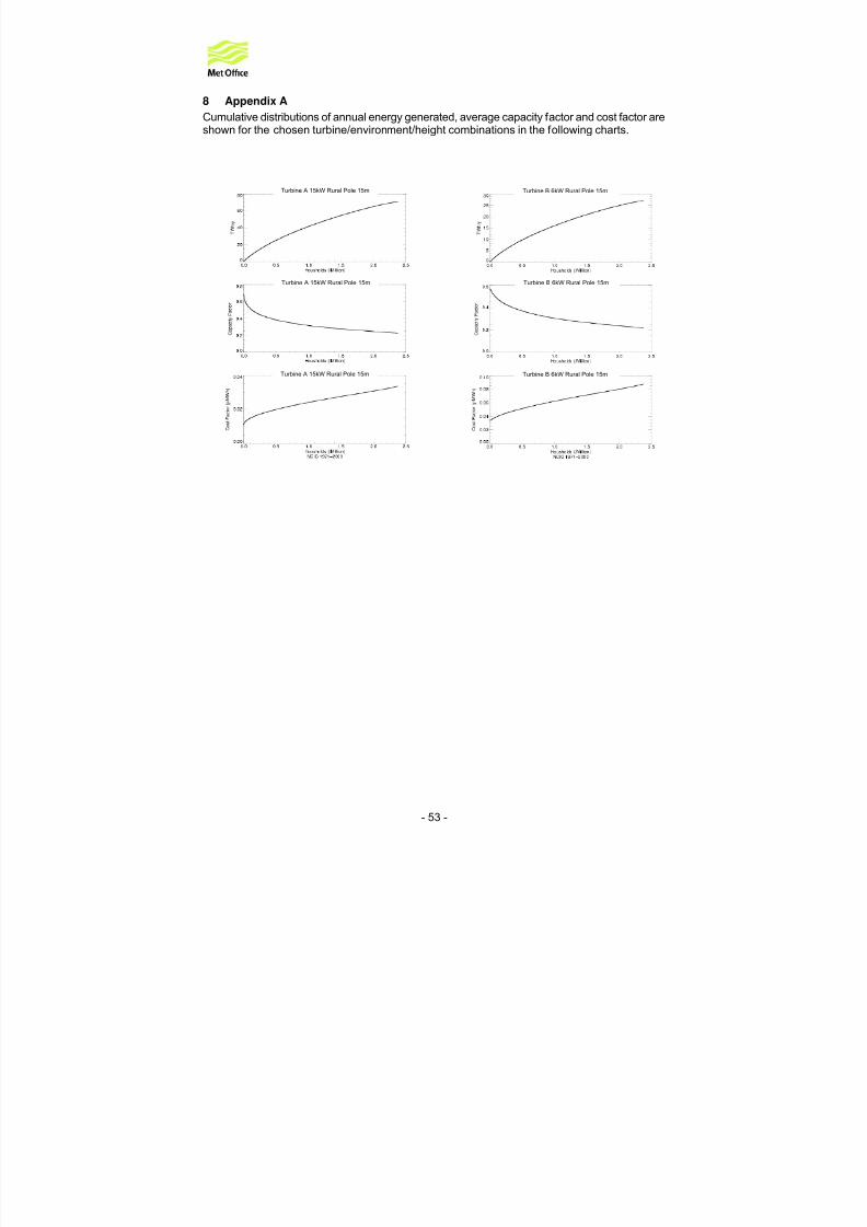
8/6/2019 Best Et Al._small-Scale Wind Energy Technical Report_2008
http://slidepdf.com/reader/full/best-et-alsmall-scale-wind-energy-technical-report2008 185/191

8/6/2019 Best Et Al._small-Scale Wind Energy Technical Report_2008
http://slidepdf.com/reader/full/best-et-alsmall-scale-wind-energy-technical-report2008 186/191
- 54 -
Turbine C 2.5kW Rural Pole 11m Turbine D 0.08kW Rural Pole 11m
Turbine C 2.5kW Rural Pole 11m Turbine D 0.08kW Rural Pole 11m
Turbine C 2.5kW Rural Pole 11m Turbine D 0.08kW Rural Pole 11m
Turbine E 2.4kW Urban Pole 10m Turbine E 2.4kW Suburban Pole 10m
Turbine E 2.4kW Urban Pole 10m Turbine E 2.4kW Suburban Pole 10m
Turbine E 2.4kW Urban Pole 10m Turbine E 2.4kW Suburban Pole 10m
8/6/2019 Best Et Al._small-Scale Wind Energy Technical Report_2008
http://slidepdf.com/reader/full/best-et-alsmall-scale-wind-energy-technical-report2008 187/191
- 55 -
Turbine F 1.5kW Urban Roof 1.95m Turbine F 1.5kW Suburban Roof 1.95m
Turbine F 1.5kW Urban Roof 1.95m Turbine F 1.5kW Suburban Roof 1.95m
Turbine F 1.5kW Urban Roof 1.95m Turbine F 1.5kW Suburban Roof 1.95m
Turbine F 1.5kW Urban Roof 2.95m Turbine F 1.5kW Suburban Roof 2.95m
Turbine F 1.5kW Urban Roof 2.95m Turbine F 1.5kW Suburban Roof 2.95m
Turbine F 1.5kW Urban Roof 2.95m Turbine F 1.5kW Suburban Roof 2.95m
8/6/2019 Best Et Al._small-Scale Wind Energy Technical Report_2008
http://slidepdf.com/reader/full/best-et-alsmall-scale-wind-energy-technical-report2008 188/191
- 56 -
Turbine F 1.5kW Urban Roof 8.95m
Turbine F 1.5kW Urban Roof 8.95m
Turbine F 1.5kW Urban Roof 8.95m
Turbine F 1.5kW Suburban Roof 8.95m
Turbine F 1.5kW Suburban Roof 8.95m
Turbine F 1.5kW Suburban Roof 8.95m
Turbine G 1kW Suburban Roof 2.125m
Turbine G 1kW Suburban Roof 2.125m
Turbine G 1kW Suburban Roof 2.125m
Turbine G 1kW Urban Roof 2.125m
Turbine G 1kW Urban Roof 2.125m
Turbine G 1kW Urban Roof 2.125m

8/6/2019 Best Et Al._small-Scale Wind Energy Technical Report_2008
http://slidepdf.com/reader/full/best-et-alsmall-scale-wind-energy-technical-report2008 189/191
- 57 -
Turbine G 1kW Urban Roof 3.125m Turbine G 1kW Suburban Roof 3.125m
Turbine G 1kW Urban Roof 3.125m Turbine G 1kW Suburban Roof 3.125m
Turbine G 1kW Urban Roof 3.125m Turbine G 1kW Suburban Roof 3.125m
Turbine G 1kW Urban Roof 9.125m Turbine G 1kW Suburban Roof 9.125m
Turbine G 1kW Urban Roof 9.125m Turbine G 1kW Suburban Roof 9.125m
Turbine G 1kW Urban Roof 9.125m Turbine G 1kW Suburban Roof 9.125m

8/6/2019 Best Et Al._small-Scale Wind Energy Technical Report_2008
http://slidepdf.com/reader/full/best-et-alsmall-scale-wind-energy-technical-report2008 190/191
- 58 -
9 References
Alexander, L., Tett, S. & Jonsson, T. (2005): Recent observed changes in severe storms over the United Kingdom and Iceland. Geophys Res Lett, 32, L13704. doi:10.1029/2005GL022371
Christensen, J.H., B. Hewitson, A. Busuioc, A. Chen, X. Gao, I. Held, R. Jones, R.K. Kolli, W.-T.Kwon, R. Laprise, V. Magaña Rueda, L. Mearns, C.G. Menéndez, J. Räisänen, A. Rinke, A. Sarr and P. Whetton, 2007: Regional Climate Projections. In: Climate Change 2007: The PhysicalScience Basis. Contribution of Working Group I to the Fourth Assessment Report of theIntergovernmental Panel on Climate Change [Solomon, S., D. Qin, M. Manning, Z. Chen, M.Marquis, K.B. Averyt, M. Tignor and H.L. Miller (eds.)]. Cambridge University Press, Cambridge,United Kingdom and New York, NY, USA.
Grimmond, C.S.B. & Oke, T.R., Aerodynamic properties of urban areas derived from analysis of surface form, J. Applied Meteorol. , 38 , 1262-1292 (1999)
(see also Grimmond, C.S.B. & Oke, T.R., Corrigendum, J. Applied Meteorol. , 39 , 2494 (2000))Harrison, G.P., Cradden, L.C., Chick, J.P., Preliminary assessment of climate change impactson the UK onshore wind energy resource, Invited paper for Special Issue of “Energy Sources” onGlobal Climate Change and Sustainable Energy Development, 2007 Available athttp://www.see.ed.ac.uk/~gph/publications/EnergySourcesDraft.pdf
Heath, M.A., Walshe, J.D. and Watson S.J., Estimating the potential yield of small building-mounted wind turbines, Wind Energy , 10 , 271-287 (2007)
Hulme, M., Jenkins, G.J., Lu, X., Turnpenny, J.R., Mitchell, T.D., Jones, R.G., Lowe, J., Murphy,J.M., Hassell, D., Boorman, P., McDonald, R. and Hill, S. (2002) Climate Change Scenarios for
the United Kingdom: The UKCIP02 Scientific Report, Tyndall Centre for Climate ChangeResearch, University of East Anglia, Norwich, UK. 120pp.
Macdonald, R.W., Griffiths, R.F. & Hall, D.J., An improved method for the estimation of surfaceroughness of obstacle arrays, Atmos. Environment , 32 , 1857-1864 (1998)
Raupach, M. R., Simplified expressions for vegetation roughness length and zero-planedisplacement as functions of canopy height and area index, Boundary-Layer Meteorol. , 71 , 211-216 (1994)
Raupach, M. R., Corrigenda, Boundary-Layer Meteorol. , 76 , 303-304 (1995)
Troen, I and Petersen, E, European Wind Atlas, Risø National Laboratory, Roskilde, Denmark,656pp (1989)

8/6/2019 Best Et Al._small-Scale Wind Energy Technical Report_2008
http://slidepdf.com/reader/full/best-et-alsmall-scale-wind-energy-technical-report2008 191/191