Embed Size (px)
Citation preview
Mathematical Researches Vol. 2, No. 1 Spring & Summer 2016 17
(Sci. Kharazmi University)
Bernoulli Wavelets Method for Solution of Fractional
Differential Equations in a Large Interval
Keshavarz E., *Ordokhani Y.;
Faculty of Mathematical Sciences, Alzahra University Received: 18 Nov 2013 Revised: 10 Nov 2014
Abstract
In this paper, Bernoulli wavelets are presented for solving (approximately) fractional
differential equations in a large interval. Bernoulli wavelets operational matrix of fractional
order integration is derived and utilized to reduce the fractional differential equations to
system of algebraic equations. Numerical examples are carried out for various types of
problems, including fractional Van der Pol and Bagley-Torvik equations for the application
of the method. Illustrative examples are presented to demonstrate the efficiency and
accuracy of the proposed method.
Keywords: Bernoulli wavelet, Fractional calculus, Differential equations, Block pulse function, Van der
Pol equation, Bagley-Torvik equation, Caputo derivative, Operational matrix, Numerical solution
Introduction
In recent decades, applied scientists and engineers have realized that fractional
differential equations (FDEs) provide a better approach to describing the complex
phenomena in nature such as non-Brownian motion, signal processing, systems
identification, control, viscoelastic materials and polymers [1–3].
In general, it is not easy to derive the analytical solutions to most of the FDEs.
Therefore, it is vital to develop some reliable and efficient techniques to solve FDEs.
Numerical solution of FDEs has attracted considerable attention from many researchers.
During the past decades, an increasing number of numerical schemes have been
developed. These methods include fractional linear multi-step methods [4,5], the
Adomian decomposition method [6–8], variational iteration method [9, 10], operational
matrix method [11–22] and Homotopy analysis method [23–26].
Numerical solutions of the FDEs in a large interval have been investigated by some
researchers. There are few references on the solution for fractional Van der Pol
*Corresponding author: [email protected]
Dow
nloa
ded
from
mm
r.kh
u.ac
.ir a
t 18:
02 IR
ST
on
Frid
ay J
anua
ry 1
0th
2020
18 Vol. 2, No. 1 Spring & Summer 2016 Mathematical Researches (Sci. Kharazmi University)
equations [27, 28] and Bagley-Torvik equations [29]. In this paper we solve the two
above noted equations. We introduce a new direct computational method to solve them.
The method consists of using Bernoulli wavelet operational matrix of fractional order
integration to reduce the FDEs to a set of algebraic equations. For approximating an
arbitrary time functions the advantages of Bernoulli polynomials )(tm , 0,1,2,=m
where 10 t over shifted Legendre polynomials are given in [30–32].
The rest of the paper is organized as follows: in section 2, basic definitions of
fractional calculus, Bernoulli wavelets and their properties are introduced. In section 3,
how to derive Bernoulli wavelet operational matrix of fractional order integration is
given. Illustrative examples are given in section 4 to demonstrate the application of
operational matrix of fractional order integration for Bernoulli wavelets. Finally, we
present the conclusion in section 5.
Preliminaries and notations
1. The fractional integral and derivative
In this section, we first state some definitions and basic properties regarding
fractional derivatives and integral. There are various definitions of fractional integration
and differentiation, such as Grunwald-Letnikov’s definition and Riemann-Liouville’s
definition. To solve differential equations (both classical and fractional), we need to
specify additional conditions in order to produce a unique solution. For the case of the
Caputo FDEs, the additional conditions are just the traditional conditions, which are
akin to those of classical differential equations, and are therefore familiar to us. In
contrast, for the Riemann-Liouville FDEs, the additional conditions constitute certain
fractional derivatives (and/or integrals) of the unknown solution at the initial point 0=t
, which are functions of t . These initial conditions are not physical, furthermore, it is
not clear how such quantities are to be measured from experiment, say, so that they can
be appropriately assigned in an analysis. For more details see [33]. Therefore, we use
the fractional derivatives in the Caputo sense.
Definition 1. We define
1( ) ( ) 0, 0, ( ) ( )pC f t f t t f t t f t , where p and 1( ) [0, )f t C ,
( )( ) ( )n nC f t f t C , where n and .
Definition 2. The Riemann-Liouville fractional integral operator of order 0q , of a
function ( )f t C , 1 , is defined as [34]
Dow
nloa
ded
from
mm
r.kh
u.ac
.ir a
t 18:
02 IR
ST
on
Frid
ay J
anua
ry 1
0th
2020
Bernoulli wavelets method for solution of fractional differential equations in a large interval 19
0.=),(
0,>,)(
)(
)(
1
=)( 10
qtf
qdsst
sf
qtfI q
t
q
For the Riemann-Liouville fractional integral we have
1.> ,)1(
1)(=
qq tq
tI
The Riemann-Liouville fractional integral is a linear operation, namely:
),()(=))()(( tgItfItgtfI qqq
where and are constants.
Definition 3. Caputo’s fractional derivative of order q , for the function 1( ) nf t C , is
defined as [35]
, ,<1 ,)(
)(
)(
1=)(
1
)(
0
nnqndsst
sf
qntfD
nq
ntq
where 0>q is the order of the derivative and n is the smallest integer greater than or
equal q .
For the Caputo derivative we have the following two basic properties [36]
),(=)( tftfID qq
and
.!
(0))(=)( )(1
0= i
tftftfDI
ii
n
i
(1)
2. The properties of Bernoulli wavelets
2.1. Wavelets and Bernoulli wavelets
Wavelets are a family of functions constructed from dilation and translation of a single
function called the mother wavelet. When the dilation parameter a and the translation
parameter b vary continuously we have the following family of continuous wavelets as
[37]
0.,, ),(||=)( 2
1
,
abaa
btatba
If we restrict the parameters a and b to discrete values as kaa
0= , kanbb
00= , 1>0a ,
1>0b , where n and k are positive integers, the family of discrete wavelets are defined
as
),(||=)( 002
0, nbtaat k
k
nk
Dow
nloa
ded
from
mm
r.kh
u.ac
.ir a
t 18:
02 IR
ST
on
Frid
ay J
anua
ry 1
0th
2020
20 Vol. 2, No. 1 Spring & Summer 2016 Mathematical Researches (Sci. Kharazmi University)
where )(, tnk form a wavelet basis for )(2 L .
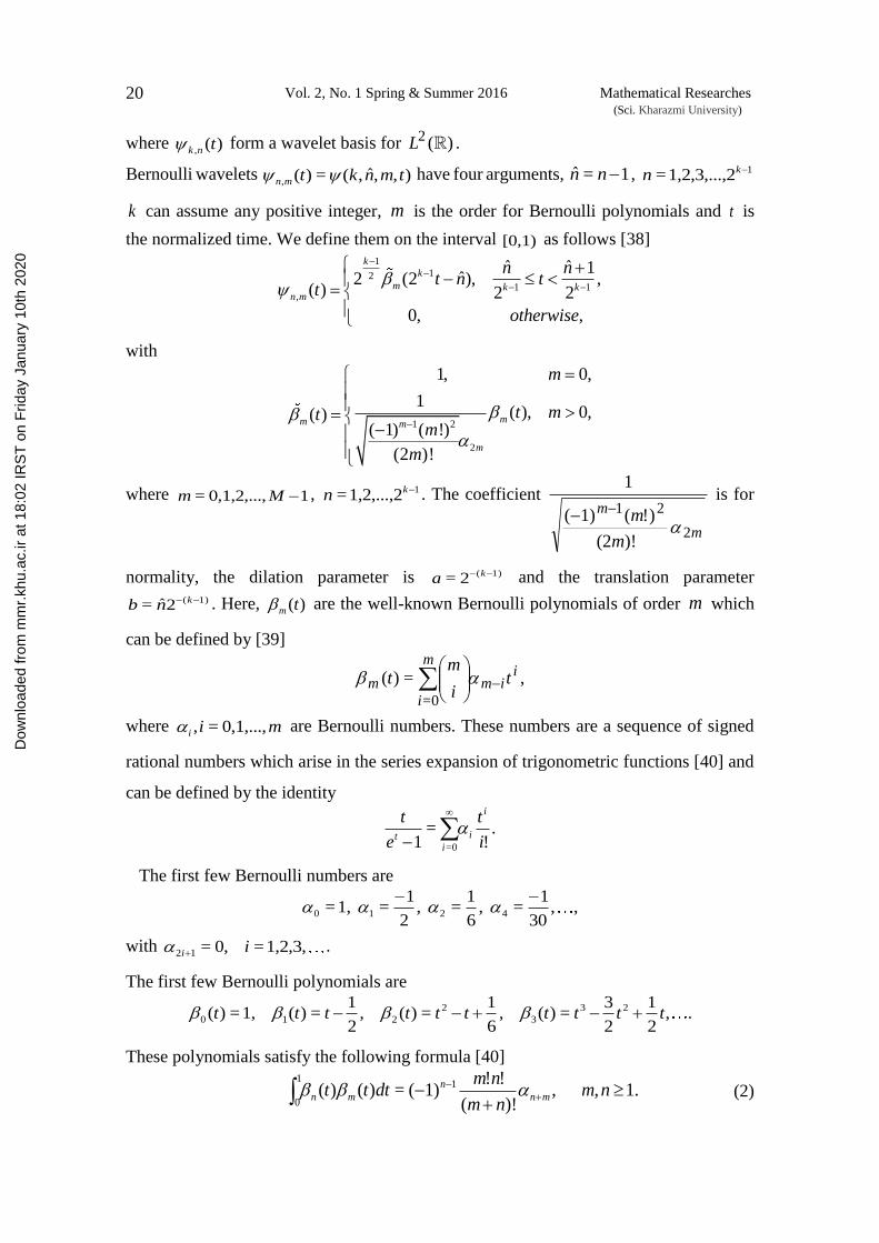
Bernoulli wavelets ),,ˆ,(=)(, tmnktmn have four arguments, 1=ˆ nn , 121,2,3,...,= kn
k can assume any positive integer, m is the order for Bernoulli polynomials and t is
the normalized time. We define them on the interval [0,1) as follows [38] 1
121 1
,
ˆ ˆ 1ˆ2 (2 ), ,
( ) 2 2
0, ,
k
k
m k kn m
n nt n t
t
otherwise
with
1 2
2
1, 0,
1( ), 0,( )
( 1) ( !)
(2 )!
mm m
m
m
t mtm
m
where 10,1,2,...,= Mm , 11,2,...,2= kn . The coefficient
m
m
m
m2
21
)!(2
)!(1)(
1
is for
normality, the dilation parameter is 1)(2= ka and the translation parameter
1)(2ˆ= knb . Here, )(tm are the well-known Bernoulli polynomials of order m which
can be defined by [39]
,=)(
0=
iim
m
i
m ti
mt
where mii 0,1,...,=, are Bernoulli numbers. These numbers are a sequence of signed
rational numbers which arise in the series expansion of trigonometric functions [40] and
can be defined by the identity
.!
=1 0= i
t
e
t i
i
it
The first few Bernoulli numbers are
,,30
1= ,
6
1= ,
2
1= 1,= 4210
with 1,2,3,=0,=12 ii .
The first few Bernoulli polynomials are
.,2
1
2
3=)( ,
6
1=)( ,
2
1=)( 1,=)( 23
3
2
210 tttttttttt
These polynomials satisfy the following formula [40]
1., ,)!(
!!1)(=)()( 1
1
0
nmnm
nmdttt mn
n
mn (2)
Dow
nloa
ded
from
mm
r.kh
u.ac
.ir a
t 18:
02 IR
ST
on
Frid
ay J
anua
ry 1
0th
2020
Bernoulli wavelets method for solution of fractional differential equations in a large interval 21
According to [41], Bernoulli polynomials form a complete basis over the interval [0,1] .
2.2. Function approximation
Suppose that [0,1])}(,),(),({ 2
1121110 LtttMk is the set of Bernoulli
wavelets,
)},(,),(,),(,),(),(,),(),({=1120121220111110 tttttttspanY
MkkMM
and )(tf be an arbitrary element in [0,1]2L . Since Y is a finite dimensional vector
space, )(tf has the best approximation out of Y such as Ytf )(0, that is
.)()()()( ,)( 0 tytftftfYty
Since ,)(0 Ytf there exists unique coefficients 1121110 ,...,, Mkccc such that
),(=)(=)()(1
0=
12
1=
0 tCtctftf Tnmnm
M
m
k
n
(3)
where T indicates transposition, C and )(t are 12 1 Mk matrices given by
,],,,,,,,,,,[=1120121220111110
T
MkkMM cccccccC
.)](,),(,),(,),(),(,),(),([=)(1120121220111110
T
MkkMM tttttttt
Using Eq. (3) we obtain
1,,0,1,= ,,21,2,= ,>=)(),(=< 11
0=
12
1=
1
0=
12
1=
Mjidcttcf kij
nmnm
M
m
k
n
ijnmnm
M
m
k
n
ij
that >)(),(=< ttff ijij , >)(),(=< ttd ijnm
ij
nm , and ><, denotes inner product.
Therefore,
1,,0,1,= ,,21,2,=
,],,,,,,,,,,[=1
1120121220111110
Mji
dddddddCfk
Tij
Mk
ij
k
ij
M
ijij
M
ijijT
ij
or
,= DCF TT
where
,],,,,,,,,,,[=1120121220111110
T
MkkMM fffffffF
and
],[= ij
nmdD
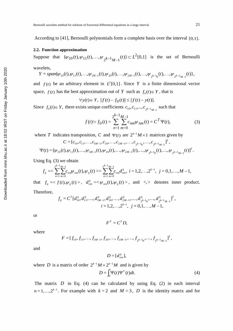
where D is a matrix of order MM kk 11 22 and is given by
.)()(=1
0dtttD T (4)
The matrix D in Eq. (4) can be calculated by using Eq. (2) in each interval
1,21,= kn . For example with 2=k and 3=M , D is the identity matrix and for
Dow
nloa
ded
from
mm
r.kh
u.ac
.ir a
t 18:
02 IR
ST
on
Frid
ay J
anua
ry 1
0th
2020
22 Vol. 2, No. 1 Spring & Summer 2016 Mathematical Researches (Sci. Kharazmi University)
2=k and 4=M we have
1 0 0 0 0 0 0 0
70 1 0 0 0 0 0
10
0 0 1 0 0 0 0 0
70 0 1 0 0 0 0
10.
0 0 0 0 1 0 0 0
70 0 0 0 0 1 0
10
0 0 0 0 0 0 1 0
70 0 0 0 0 0 1
10
D
Therefore, TC in Eq. (3) is given by
.= 1DFC TT
Bernoulli wavelet operational matrix of the fractional integration
In this section, we define the Bernoulli wavelet matrix. Then, by using the Block-
Pulse operational matrix of fractional integration, we derive the Bernoulli wavelet
operational matrix of the fractional integration.
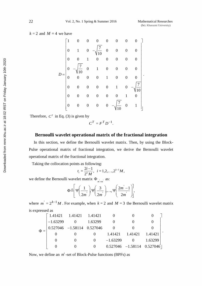
Taking the collocation points as following:
,,21,2,= ,2
12= 1Mi
M
it k
ki
we define the Bernoulli wavelet matrix '' mm as:
,2
12,,
2
3,
2
1
'
'
''
m
m
mm
where Mm k 1' 2= . For example, when 2=k and 3=M the Bernoulli wavelet matrix
is expressed as
1.41421 1.41421 1.41421 0 0 0
1.63299 0 1.63299 0 0 0
0.527046 1.58114 0.527046 0 0 0= .
0 0 0 1.41421 1.41421 1.41421
0 0 0 1.63299 0 1.63299
0 0 0 0.527046 1.58114 0.527046
Now, we define an m -set of Block-Pulse functions (BPFs) as
Dow
nloa
ded
from
mm
r.kh
u.ac
.ir a
t 18:
02 IR
ST
on
Frid
ay J
anua
ry 1
0th
2020
Bernoulli wavelets method for solution of fractional differential equations in a large interval 23
,0,
,1
<1,=)(
otherwisem
it
m
i
tbi
where 1,0,1,2,= mi . BPFs have the following useful property
.=),(
,0,=)()(
jitb
jitbtb
iji (5)
Bernoulli wavelets may be expanded into an m -term BPFs as
),(=)( tBt (6)
where Tm tbtbtbtB )](,),(),([)( 110 . Kilicman and Al Zhour have given the Block-
Pulse operational matrix of the fractional integration )(qF as following [42]:
),(=)( )( tBFtBI qq (7)
where
1 2 1
1 2
( )
3
1
0 11 1
= ,0 0 1( 2)
0 0 0
0 0 0 0 1
m
m
q
mqF
m q
with .1)(21)(= 111 qqq
k kkk
We now derive the Bernoulli wavelet operational matrix of fractional integration. Let
),(=)( )( tPtI qq (8)
where the matrix )(qP is called the Bernoulli wavelet operational matrix of fractional
integration. Using Eqs. (6) and (7) we get
).(=)(=)(=)( )( tBFtBItBItI qqqq (9)
From Eqs. (8) and (9) we have
).(=)(=)( )()()( tBFtBPtP qqq
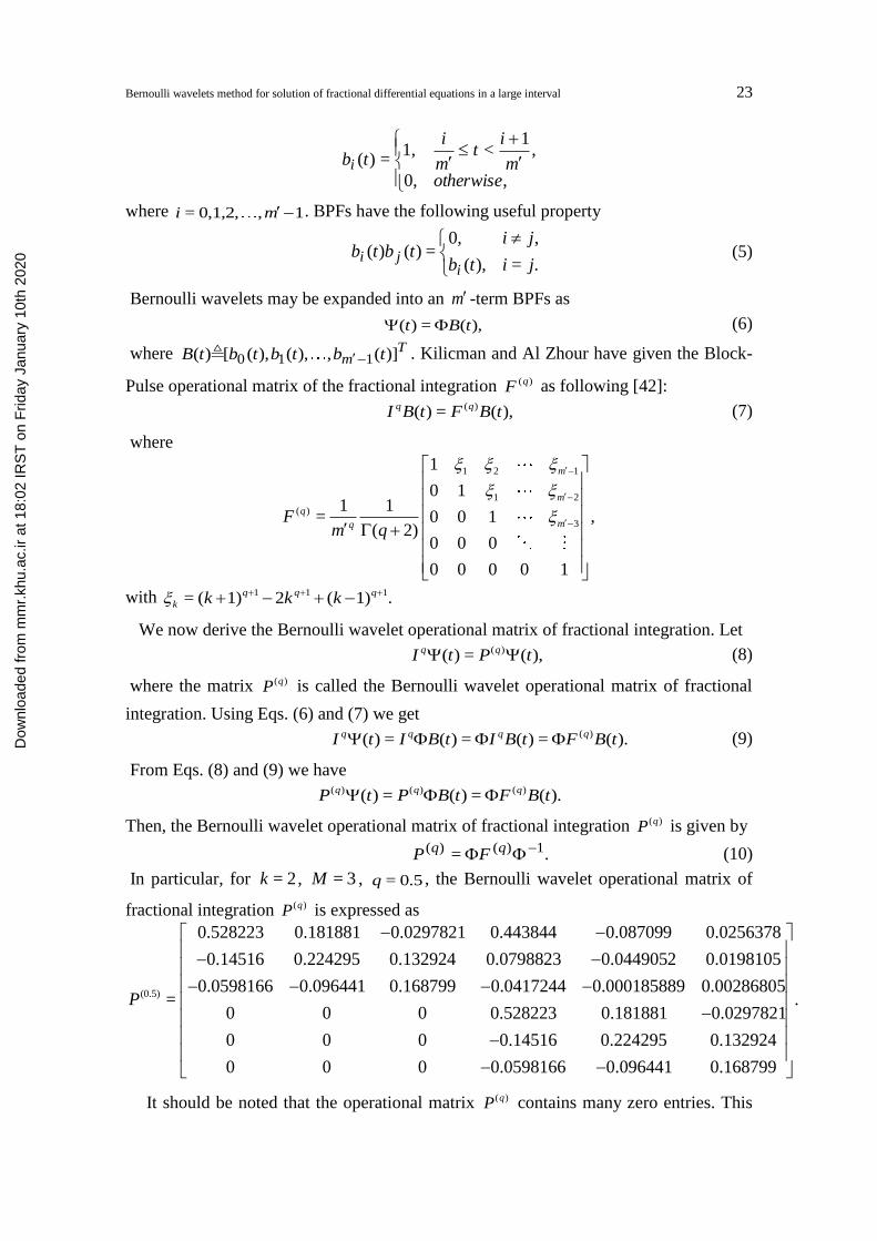
Then, the Bernoulli wavelet operational matrix of fractional integration )(qP is given by
.= 1)()( qq FP (10)
In particular, for 2=k , 3=M , 0.5=q , the Bernoulli wavelet operational matrix of
fractional integration )(qP is expressed as
(0.5)
0.528223 0.181881 0.0297821 0.443844 0.087099 0.0256378
0.14516 0.224295 0.132924 0.0798823 0.0449052 0.0198105
0.0598166 0.096441 0.168799 0.0417244 0.000185889 0.00286805=
0 0 0 0.528223 0.181881 0.0297821
0
P
.
0 0 0.14516 0.224295 0.132924
0 0 0 0.0598166 0.096441 0.168799
It should be noted that the operational matrix )(qP contains many zero entries. This
Dow
nloa
ded
from
mm
r.kh
u.ac
.ir a
t 18:
02 IR
ST
on
Frid
ay J
anua
ry 1
0th
2020
24 Vol. 2, No. 1 Spring & Summer 2016 Mathematical Researches (Sci. Kharazmi University)
phenomena makes calculations fast. The calculation for the matrix )(qP is carried out
for fixed ,k M , and is used to solve fractional order as well as integer order differential
equations.
Illustrative examples
To demonstrate the effectiveness of the method, we consider some fractional
differential equations. We use Mathematica ver. 7.0 software to solve following
examples.
Example 1. Consider the damped Van der Pol equation with fractional damping, which
is governed by the studies of Juhn-Horng Chen and Wei-Ching Chen [43] as following
2<<0 ),(=)()(1))(()( 2 qtasintxtxDtxtx q , (11)
(0) = 0 ,
(0) = 0 ,
x
x (12)
the second initial condition is for 1>q only. The initial conditions are homogeneous,
is the damping parameter, a the amplitude of periodic forcing, denotes the
forcing frequency and qD the differential operator that denotes the q -th derivative of the
related function with respect to t.
Let
),()(2 tCtxD T (13)
by using Eqs. (1), (6), (8), (10) and (12) we have
),(=)(=))((=)( 1)(2)(222 tFCtPCtxDItxD qTqTqq (14)
and
),(=)(=(0)(0))(=)( 1
(2)(2) tBAtBPCtxxtPCtx TT (15)
where
].,,,[== 110
(2)
1 m
T aaaPCA
By using Eqs. (5) and (15), we have
),(=)()()(=
)]()()([=)]([=)]([
21
2
11
2
10
2
0
2
111100
2
1
2
tBAtbatbatba
tbatbatbatBAtx
mm
mm
where
].,,,[= 2
1
2
1
2
02 maaaA
Similarly, the input signal )( tasin may be expanded by the Bernoulli wavelets as
),(=)( tFtasin T (16)
where TF is a known constant vector. Substituting Eqs. (13)–(16) in Eq. (11), we have
Dow
nloa
ded
from
mm
r.kh
u.ac
.ir a
t 18:
02 IR
ST
on
Frid
ay J
anua
ry 1
0th
2020
Bernoulli wavelets method for solution of fractional differential equations in a large interval 25
0.=)()(
)()()()((2)
1)(21)(2
2
tFtPC
tFCtFCtBAtCTT
qTqTT
(17)
To find the solution )(tx , we first collocate Eq. (17) at the points M
it
ki2
12=
,
Mi k 1,21,2,= . These equations generate Mk 12 algebraic equations which can be
solved by using Newton’s iterative method. Consequently, )(tx given in Eq. (15) can
be calculated approximately.
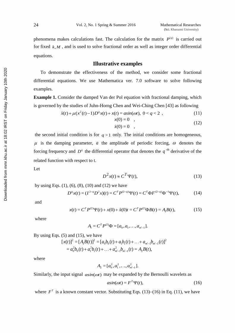
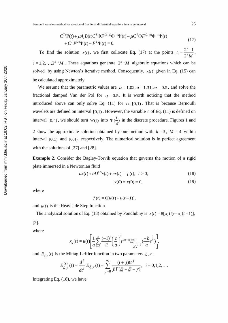
We assume that the parametric values are 0.5= 1.31,= 1.02,= a , and solve the
fractional damped Van der Pol for 0.5=q . It is worth noticing that the method
introduced above can only solve Eq. (11) for [0,1)t . That is because Bernoulli
wavelets are defined on interval [0,1) . However, the variable t of Eq. (11) is defined on
interval [0,4) , we should turn )(t into )4
(t
in the discrete procedure. Figures 1 and
2 show the approximate solution obtained by our method with 3=k , 4=M within
interval [0,1) and [0,4) , respectively. The numerical solution is in perfect agreement
with the solutions of [27] and [28].
Example 2. Consider the Bagley-Torvik equation that governs the motion of a rigid
plate immersed in a Newtonian fluid
0,> ),(=)()()( 1.5 ttftcxtxbDtxa (18)
0,=(0)=(0) xx (19)
where
1)],()(8[=)( tututf
and )(tu is the Heaviside Step function.
The analytical solution of Eq. (18) obtained by Pondlubny is 1)],()(8[=)( txtxtx uu
[2].
where
,)(!
1)(1)(=)( 2
1
)(
32
3,
2
1
1)2(
0=
ta
bEt
a
c
iatutx i
i
i
ii
i
u
and )(, tE is the Mittag-Leffler function in two parameters , :
. 0,1,2,= ,)(!
)!(=)(=)(
0=
,)(,
iijj
tjitE
dt
dtE
j
ji
ii
Integrating Eq. (18), we have
Dow
nloa
ded
from
mm
r.kh
u.ac
.ir a
t 18:
02 IR
ST
on
Frid
ay J
anua
ry 1
0th
2020
26 Vol. 2, No. 1 Spring & Summer 2016 Mathematical Researches (Sci. Kharazmi University)
Figure 1. Approximate solution within interval [0,1) , for Example 4.1
Figure 2. Approximate solution within interval [0,4) , for Example 4.1
).(=)()((0)](0))([ 220.5 tfItxcItxbIxtxtxa (20)
Let
).()( tCtx T (21)
Similarly, the input signal )(tf may be expanded by the Bernoulli wavelet as
).()( tFtf T (22)
Substituting Eqs. (19), (21) and (22) into (20), we have
0,=)()()()( 220.5 tIFtIcCtIbCtaC TTTT
then by using Eq. (8) we have
0,=)()()()( (2)(2)(0.5) tPFtPcCtPbCtaC TTTT
or
0,=(2)(2)(0.5) PFPcCPbCaC TTTT
then
.][= 1(2)(0.5)(2) cPbPaIPFC TT
0.0 0.2 0.4 0.6 0.8 1.0
0.00
0.02
0.04
0.06
0.08
0.10
0 1 2 3 40.0
0.5
1.0
1.5
2.0
Dow
nloa
ded
from
mm
r.kh
u.ac
.ir a
t 18:
02 IR
ST
on
Frid
ay J
anua
ry 1
0th
2020
Bernoulli wavelets method for solution of fractional differential equations in a large interval 27
Finding the unknown coefficient vector C , given in Eq. (21) can be calculated.
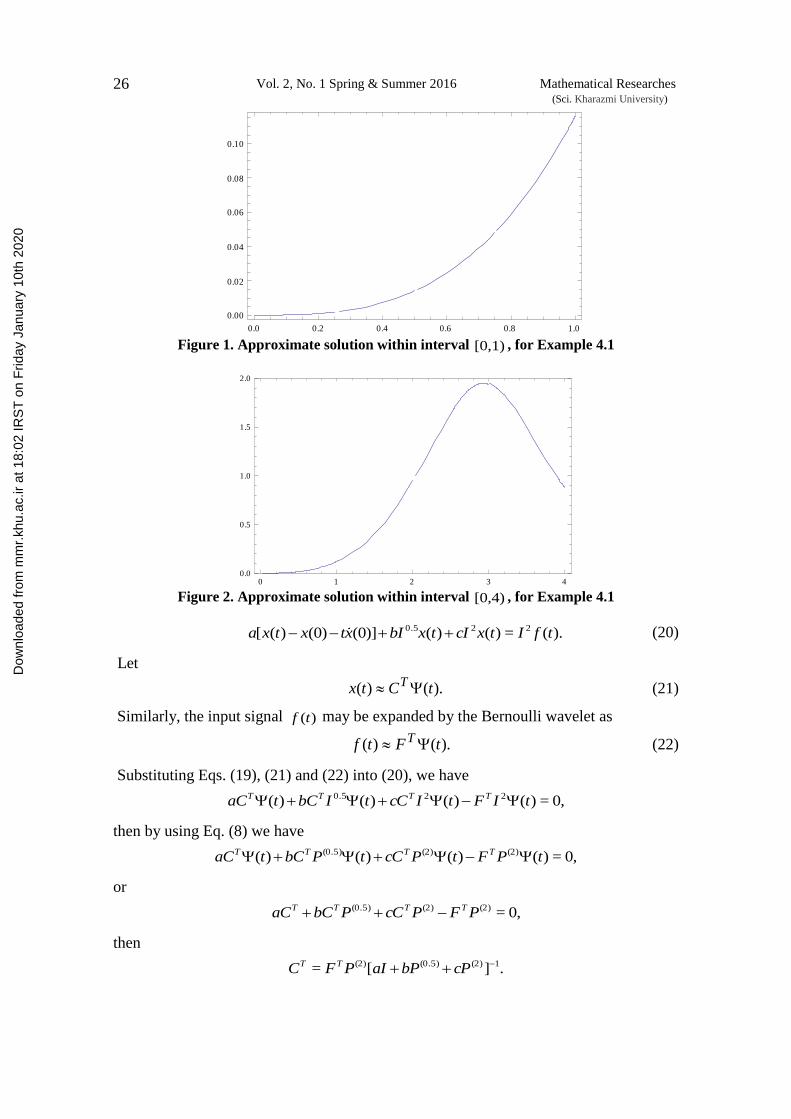
We assume that 0.5= 0.5,= 1,= cba , and solve Eq. (18) with 4=4,= Mk . Figure 3
shows the numerical solution (on the interval [0,20) method is the same as Example 4.1)
that is in very good agreement with the exact solution. This demonstrates the
importance of our numerical scheme in solving nonlinear multi-order fractional
differential equations. Also, Table 1 shows the absolute error of )(tx for our method
and Haar wavelet [29].
Figure 3. Numerical and exact solution within interval [0,20) , for Example 4.2
Table 1. Absolute error of )(tx , for Example 4.2
t Haar wavelet [29] Bernoulli wavelet
1 0.585974 0.124625
2 0.77707 0.00429792
3 0.61926 0.0414732
4 0.184014 0.0645971
5 0.41339 0.0347576
6 0.966783 0.029914
7 1.26268 0.0161954
8 1.17045 0.00931825
9 0.697989 0.00940264
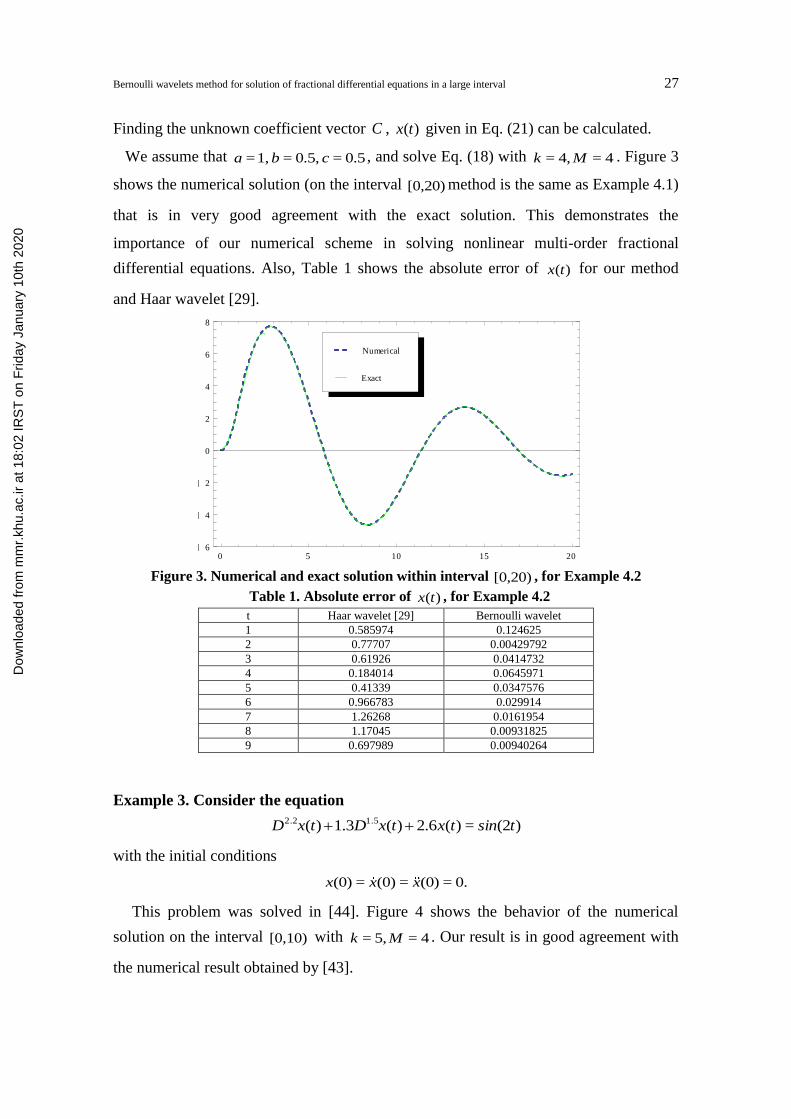
Example 3. Consider the equation
)(2=)(2.6)(1.3)( 1.52.2 tsintxtxDtxD
with the initial conditions
0.=(0)=(0)=(0) xxx
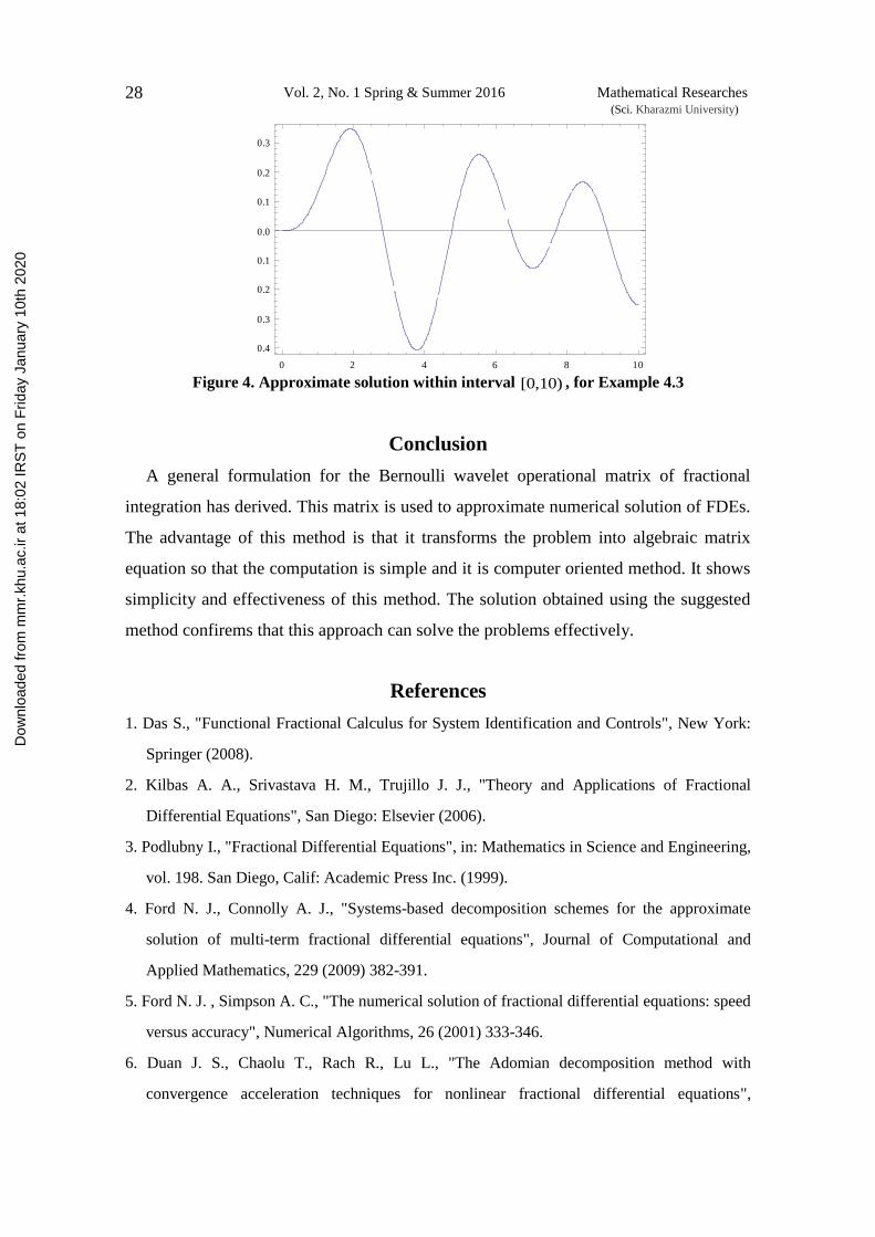
This problem was solved in [44]. Figure 4 shows the behavior of the numerical
solution on the interval [0,10) with 4=5,= Mk . Our result is in good agreement with
the numerical result obtained by [43].
)(tx
0 5 10 15 206
4
2
0
2
4
6
8
Exact
Numerical
Dow
nloa
ded
from
mm
r.kh
u.ac
.ir a
t 18:
02 IR
ST
on
Frid
ay J
anua
ry 1
0th
2020
28 Vol. 2, No. 1 Spring & Summer 2016 Mathematical Researches (Sci. Kharazmi University)
Figure 4. Approximate solution within interval [0,10) , for Example 4.3
Conclusion
A general formulation for the Bernoulli wavelet operational matrix of fractional
integration has derived. This matrix is used to approximate numerical solution of FDEs.
The advantage of this method is that it transforms the problem into algebraic matrix
equation so that the computation is simple and it is computer oriented method. It shows
simplicity and effectiveness of this method. The solution obtained using the suggested
method confirems that this approach can solve the problems effectively.
References
1. Das S., "Functional Fractional Calculus for System Identification and Controls", New York:
Springer (2008).
2. Kilbas A. A., Srivastava H. M., Trujillo J. J., "Theory and Applications of Fractional
Differential Equations", San Diego: Elsevier (2006).
3. Podlubny I., "Fractional Differential Equations", in: Mathematics in Science and Engineering,
vol. 198. San Diego, Calif: Academic Press Inc. (1999).
4. Ford N. J., Connolly A. J., "Systems-based decomposition schemes for the approximate
solution of multi-term fractional differential equations", Journal of Computational and
Applied Mathematics, 229 (2009) 382-391.
5. Ford N. J. , Simpson A. C., "The numerical solution of fractional differential equations: speed
versus accuracy", Numerical Algorithms, 26 (2001) 333-346.
6. Duan J. S., Chaolu T., Rach R., Lu L., "The Adomian decomposition method with
convergence acceleration techniques for nonlinear fractional differential equations",
0 2 4 6 8 10
0.4
0.3
0.2
0.1
0.0
0.1
0.2
0.3
Dow
nloa
ded
from
mm
r.kh
u.ac
.ir a
t 18:
02 IR
ST
on
Frid
ay J
anua
ry 1
0th
2020
Bernoulli wavelets method for solution of fractional differential equations in a large interval 29
Computers and Mathematics with Applications, 66(5) (2013) 728-736.
7. Duan J., Chaolu T. , Rach R., "Solutions of the initial value problem for nonlinear fractional
ordinary differential equations by the Rach-Adomian-Meyers modified decomposition
method", Applied Mathematics and Computation, 218(17) (2012) 8370-8392.
8. Song L., Wang W., "A new improved Adomian decomposition method and its application to
fractional differential equations", Applied Mathematical Modelling, 37 (3) (2013) 1590-
1598.
9. Wu G. C., "A fractional variational iteration method for solving fractional nonlinear
differential equations", Computers and Mathematics with Applications, 61(8) (2011) 2186-
2190.
10. Yang S., Xiao A., Su H., "Convergence of the variational iteration method for solving multi-
order fractional differential equations", Computers and Mathematics with Applications,
60(10) (2010) 2871-2879.
11. Saadatmandi A., Dehghan M., "A new operational matrix for solving fractional-order
differential equations", Computers and Mathematics with Applications, 59 (2010) 1326-
1336.
12. Hwang C., Shih Y. P., "Laguerre operational matrices for fractional calculus and
applications", International Journal of Control, 34(3) (1981) 577-584.
13. Wang C. H., "On the generalization of block-pulse operational matrices for fractional and
operational calculus", Journal of the Franklin Institute, 315(2) (1983) 91-102.
14. Lakestani M., Dehghan M., Irandoust-pakchin S., "The construction of operational matrix of
fractional derivatives using B-spline functions", Communications in Nonlinear Science and
Numerical Simulation, 17 (2012) 1065-1064.
15. Wang M. L., Chang R. Y., Yang S. Y., "Generalization of generalized orthogonal
polynomial operational matrices for fractional and operational calculus", International
Journal of Systems Science, 18(5) (1987) 931-943.
16. Khader M. M., "Numerical solution of nonlinear multi-order fractioanl defferential
equations by implementation of the operatioanl matrix of fractional derivative", Studies in
Nonlinear Sciences, 2 (1) (2011) 5-12.
17. Rehman M., Ali Khan R., "A numerical method for solving boundary value problems for
fractional differential equations", Applied Mathematical Modelling, 36 (2012) 894-907.
Dow
nloa
ded
from
mm
r.kh
u.ac
.ir a
t 18:
02 IR
ST
on
Frid
ay J
anua
ry 1
0th
2020
30 Vol. 2, No. 1 Spring & Summer 2016 Mathematical Researches (Sci. Kharazmi University)
18. Chang R. Y., Chen K. C. , Wang M., "Modified Laguerre operational matrices for fractional
calculus and applications", International Journal of Systems Science, 16(9) (1985) 1163-
1172.
19. Yuanlu L., Ning S., "Numerical solution of fractional differential equations using the
generalized block-pulse operational matrix", Computers and Mathematics with Applications,
216 (2010) 1046-1054.
20. Atanackovic T. M., Stankovic B., "On a numerical scheme for solving differential equations
of fractional order", Mechanics Research Communications, 35 (7) (2008) 429-438.
21. Yuanlu L., Ning S., "Numerical solution of fractional differential equations using the
generalized block-pulse operational matrix", Computers and Mathematics with Applications,
216 (2010) 1046-1054.
22. Yuanlu L., Weiwei Z., "Haar wavelet operational matrix of fractional order integration and
its applications in solving the fractioanl order differntial equations", Applied Mathematics
and Computation, 216 (8) (2010) 2276-2285.
23. Odibat Z., Momani S., Xu H., "A reliable algorithm of homotopy analysis method for
solving nonlinear fractional differential equations", Applied Mathematical Modelling, 34 (3)
(2010) 593-600.
24. Hosseinnia S. H., Ranjbar A., Momani S., "Using an enhanced homotopy perturbation
method in fractional differential equations via deforming the linear part", Computers and
Mathematics with Applications, 56 (12) (2008) 3138-3149.
25. Jafari H., Das S., Tajadodi H., "Solving a multi-order fractional differential equation using
homotopy analysis method", Journal of King Saud University-Science, 23 (2) (2011) 151-
155.
26. Ganjiani M., "Solution of nonlinear fractional differential equations using homotopy
analysis method", Applied Mathematical Modelling, 34(6) (2010) 1634-1641.
27. Saha Ray S., Patra A., "Haar wavelet operational methods for the numerical solutions of
fractional order nonlinear oscillatory Van der Pol system", Applied Mathematics and
Computation, 220 (2013) 659-667.
28. Konuralp A., Konuralp C., Yildirim A., "Numerical solution to the van der Pol equation
with fractional damping", Physica Scripta, doi:10.1088/0031-8949/2009/T136/014034.
29. Saha Ray S., "On Haar wavelet operational matrix of general order and its application for
Dow
nloa
ded
from
mm
r.kh
u.ac
.ir a
t 18:
02 IR
ST
on
Frid
ay J
anua
ry 1
0th
2020
Bernoulli wavelets method for solution of fractional differential equations in a large interval 31
the numerical solution of fractional Bagley Torvik equation", Applied Mathematics and
Computation, 218 (2012) 5239-5248.
30. Mashayekhi S., Ordokhani Y., Razzaghi M., "Hybrid functions approach for nonlinear
constrained optimal control problems", Communications in Nonlinear Science and
Numerical Simulation, 17 (2012) 1831-1843.
31. Mashayekhi S., Ordokhani Y., Razzaghi M., "Hybrid functions approach for optimal control
of systems described by integro-differential equations", Applied Mathematical Modelling, 37
(2013) 3355-3368.
32. Mashayekhi S., Razzaghi M., Tripak O., "Solution of the Nonlinear Mixed Volterra-
Fredholm Integral Equations by Hybrid of Block-Pulse Functions and Bernoulli
Polynomials", The Scientific World Journal, doi:10.1155/2014/413623.
33. Podlubny I., "Geometric and physical interpretation of fractional integration and fractional
differentiation", Fractional Calculus and Applied Analysis, 5 (2002) 367-386.
34. Podlubny I., "Fractional Differential Equations: An Introduction to Fractional Derivatives",
Fractional Differential Equations, to Methods of Their Solution and Some of Their
Applications. New York: Academic Press (1998).
35. Kilbas A. A., Srivastava H. M, Trujillo J. J., "Theory and Applications of Fractional
Differential Equations", vol. 204. Elsevier: North-Holland Mathematics Studies (2006).
36. Keshavarz E., Ordokhani Y., Razzaghi M., "A numerical solution for fractional optimal
control problems via Bernoulli polynomials", Journal of Vibration and Control, 22 (18 (
(2016) 3889-3903.
37. Gu J. S., Jiang W. S., "The Haar wavelets operational matrix of integration", International
Journal of Systems Science, 27 (1996) 623-628.
38. Keshavarz E., Ordokhani Y., Razzaghi M., "Bernoulli wavelet operational matrix of
fractional order integration and its applications in solving the fractional order differential
equations", Applied Mathematical Modelling, 38 (24) (2014) 6038–6051.
39. Costabile F., Dellaccio F., Gualtieri M. I., "A new approach to Bernoulli polynomials",
Rendiconti di Matematica, Serie VII, 26 (2006) 1-12.
40. Arfken G., "Mathematical Methods for Physicists, Third edition", San Diego: Academic
press (1985).
41. Kreyszig E., "Introductory Functional Analysis with Applications", New York: John Wiley
Dow
nloa
ded
from
mm
r.kh
u.ac
.ir a
t 18:
02 IR
ST
on
Frid
ay J
anua
ry 1
0th
2020
32 Vol. 2, No. 1 Spring & Summer 2016 Mathematical Researches (Sci. Kharazmi University)
and Sons Press, 1978.
42. Kilicman A., Al Zhour Z. A. A., "Kronecker operational matrices for fractional calculus and
some applications", Applied Mathematics and Computation, 187 (1) (2007) 250-265.
43. Chen J-H., Chen W-C., "Chaotic dynamics of the fractionally damped van der Pol
equation", Chaos Solitons Fractals, 35 (2008) 188-198.
44. Arikoglu A., Ozkol I., "Solution of fractional differential equations by using differential
transform method", Chaos Solitons and Fractals, 34 (2007) 1473-1481.
45. O’Nan M., "Linear Algebra, Third edition", Harcourt College (1990).
Appendix
Lemma 1. If T is a matrix with square submatrices as
1 2
1 2
=T Z
TZ T
where the Z ’s are blocks of zeroes, then [45]
1 2.T T T .
In section 2 and 3, D and are diagonal block matrices. If blockes on the main
diagonal are vertible matrices, then using Lemma 1, there are 1D and 1 .
Dow
nloa
ded
from
mm
r.kh
u.ac
.ir a
t 18:
02 IR
ST
on
Frid
ay J
anua
ry 1
0th
2020