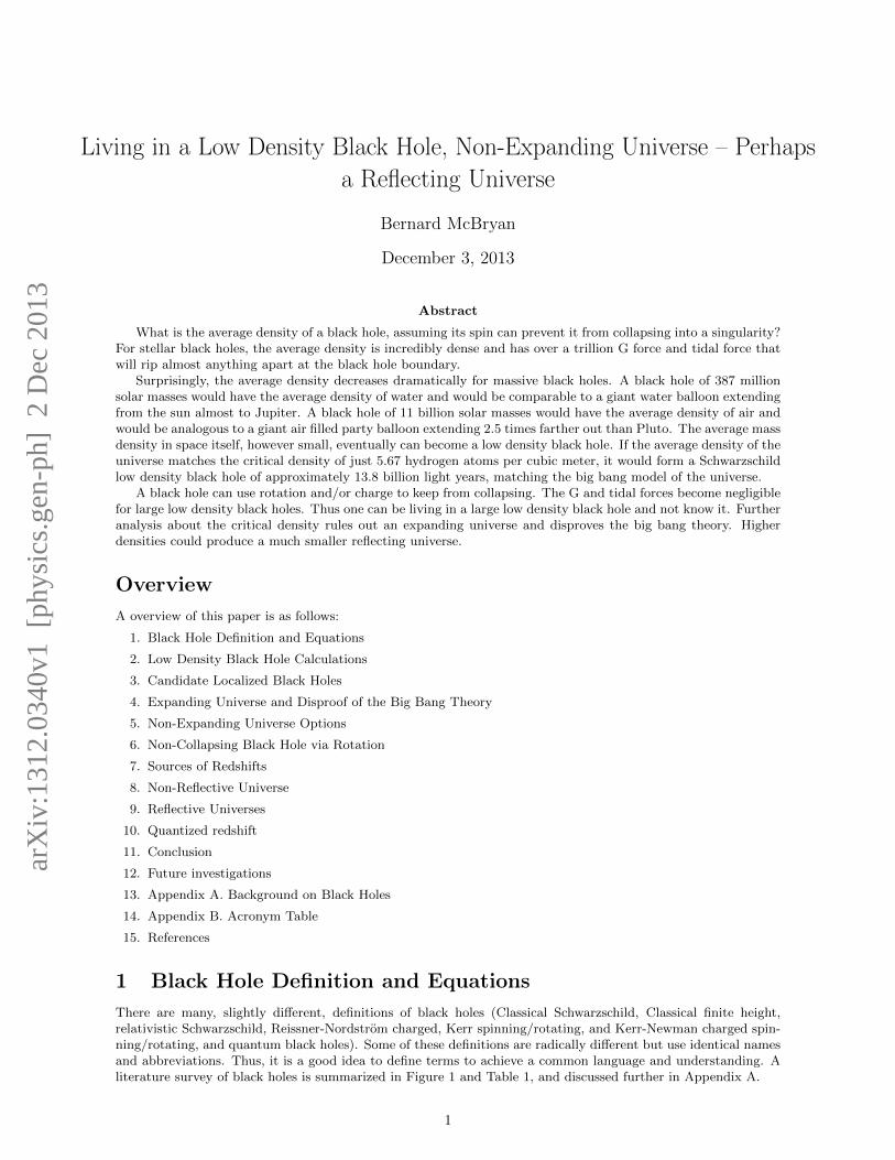
Living in a Low Density Black Hole, Non-Expanding Universe – Perhaps

a Reflecting Universe

Bernard McBryan

December 3, 2013

Abstract

What is the average density of a black hole, assuming its spin can prevent it from collapsing into a singularity?For stellar black holes, the average density is incredibly dense and has over a trillion G force and tidal force thatwill rip almost anything apart at the black hole boundary.

Surprisingly, the average density decreases dramatically for massive black holes. A black hole of 387 millionsolar masses would have the average density of water and would be comparable to a giant water balloon extendingfrom the sun almost to Jupiter. A black hole of 11 billion solar masses would have the average density of air andwould be analogous to a giant air filled party balloon extending 2.5 times farther out than Pluto. The average massdensity in space itself, however small, eventually can become a low density black hole. If the average density of theuniverse matches the critical density of just 5.67 hydrogen atoms per cubic meter, it would form a Schwarzschildlow density black hole of approximately 13.8 billion light years, matching the big bang model of the universe.

A black hole can use rotation and/or charge to keep from collapsing. The G and tidal forces become negligiblefor large low density black holes. Thus one can be living in a large low density black hole and not know it. Furtheranalysis about the critical density rules out an expanding universe and disproves the big bang theory. Higherdensities could produce a much smaller reflecting universe.

Overview

A overview of this paper is as follows:

1. Black Hole Definition and Equations

2. Low Density Black Hole Calculations

3. Candidate Localized Black Holes

4. Expanding Universe and Disproof of the Big Bang Theory

5. Non-Expanding Universe Options

6. Non-Collapsing Black Hole via Rotation

7. Sources of Redshifts

8. Non-Reflective Universe

9. Reflective Universes

10. Quantized redshift

11. Conclusion

12. Future investigations

13. Appendix A. Background on Black Holes

14. Appendix B. Acronym Table

15. References

1 Black Hole Definition and Equations

There are many, slightly different, definitions of black holes (Classical Schwarzschild, Classical finite height,relativistic Schwarzschild, Reissner-Nordstrom charged, Kerr spinning/rotating, and Kerr-Newman charged spin-ning/rotating, and quantum black holes). Some of these definitions are radically different but use identical namesand abbreviations. Thus, it is a good idea to define terms to achieve a common language and understanding. Aliterature survey of black holes is summarized in Figure 1 and Table 1, and discussed further in Appendix A.

1

arX

iv:1

312.

0340

v1 [

phys

ics.

gen-

ph]

2 D

ec 2

013

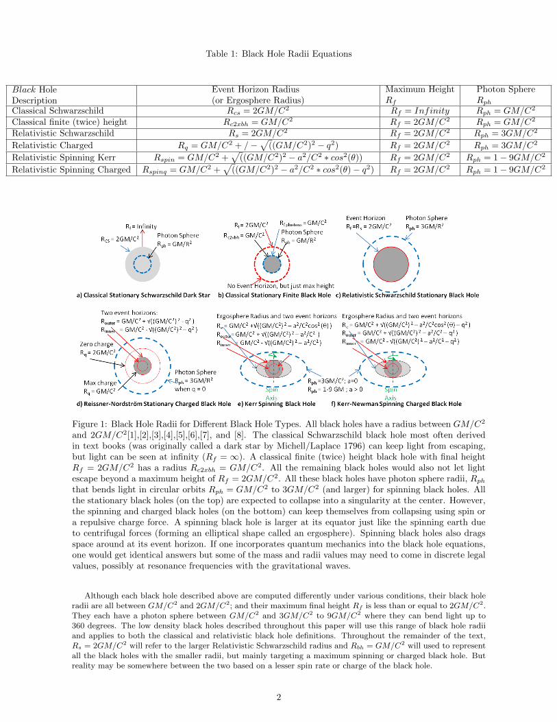
Table 1: Black Hole Radii Equations

Black HoleDescription

Event Horizon Radius(or Ergosphere Radius)

Maximum HeightRf

Photon SphereRph

Classical Schwarzschild Rcs = 2GM/C2 Rf = Infinity Rph = GM/C2

Classical finite (twice) height Rc2xbh = GM/C2 Rf = 2GM/C2 Rph = GM/C2

Relativistic Schwarzschild Rs = 2GM/C2 Rf = 2GM/C2 Rph = 3GM/C2

Relativistic Charged Rq = GM/C2 + /−√

((GM/C2)2 − q2) Rf = 2GM/C2 Rph = 3GM/C2

Relativistic Spinning Kerr Rspin = GM/C2 +√

((GM/C2)2 − a2/C2 ∗ cos2(θ)) Rf = 2GM/C2 Rph = 1− 9GM/C2

Relativistic Spinning Charged Rspinq = GM/C2 +√

((GM/C2)2 − a2/C2 ∗ cos2(θ)− q2) Rf = 2GM/C2 Rph = 1− 9GM/C2

Figure 1: Black Hole Radii for Different Black Hole Types. All black holes have a radius between GM/C2

and 2GM/C2[1],[2],[3],[4],[5],[6],[7], and [8]. The classical Schwarzschild black hole most often derivedin text books (was originally called a dark star by Michell/Laplace 1796) can keep light from escaping,but light can be seen at infinity (Rf = ∞). A classical finite (twice) height black hole with final heightRf = 2GM/C2 has a radius Rc2xbh = GM/C2. All the remaining black holes would also not let lightescape beyond a maximum height of Rf = 2GM/C2. All these black holes have photon sphere radii, Rphthat bends light in circular orbits Rph = GM/C2 to 3GM/C2 (and larger) for spinning black holes. Allthe stationary black holes (on the top) are expected to collapse into a singularity at the center. However,the spinning and charged black holes (on the bottom) can keep themselves from collapsing using spin ora repulsive charge force. A spinning black hole is larger at its equator just like the spinning earth dueto centrifugal forces (forming an elliptical shape called an ergosphere). Spinning black holes also dragsspace around at its event horizon. If one incorporates quantum mechanics into the black hole equations,one would get identical answers but some of the mass and radii values may need to come in discrete legalvalues, possibly at resonance frequencies with the gravitational waves.

Although each black hole described above are computed differently under various conditions, their black holeradii are all between GM/C2 and 2GM/C2; and their maximum final height Rf is less than or equal to 2GM/C2.They each have a photon sphere between GM/C2 and 3GM/C2 to 9GM/C2 where they can bend light up to360 degrees. The low density black holes described throughout this paper will use this range of black hole radiiand applies to both the classical and relativistic black hole definitions. Throughout the remainder of the text,Rs = 2GM/C2 will refer to the larger Relativistic Schwarzschild radius and Rbh = GM/C2 will used to representall the black holes with the smaller radii, but mainly targeting a maximum spinning or charged black hole. Butreality may be somewhere between the two based on a lesser spin rate or charge of the black hole.

2

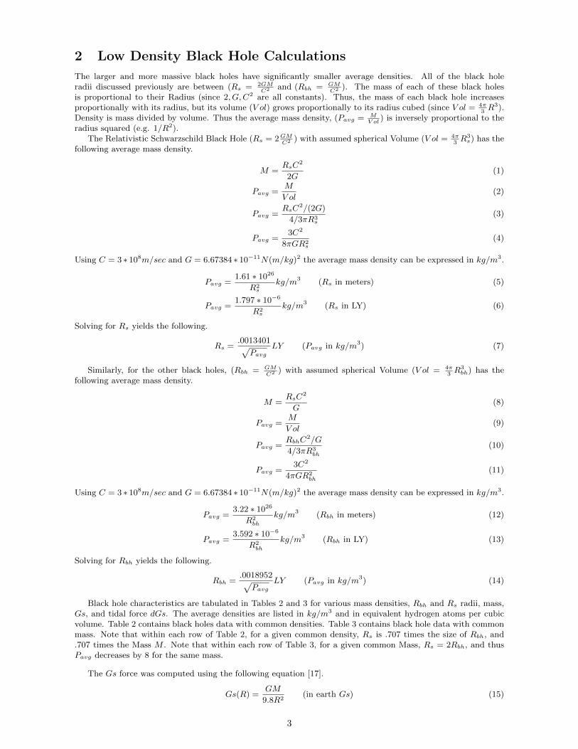
2 Low Density Black Hole Calculations

The larger and more massive black holes have significantly smaller average densities. All of the black holeradii discussed previously are between (Rs = 2GM

C2 and (Rbh = GMC2 ). The mass of each of these black holes

is proportional to their Radius (since 2, G,C2 are all constants). Thus, the mass of each black hole increasesproportionally with its radius, but its volume (V ol) grows proportionally to its radius cubed (since V ol = 4π

3R3).

Density is mass divided by volume. Thus the average mass density, (Pavg = MV ol

) is inversely proportional to theradius squared (e.g. 1/R2).

The Relativistic Schwarzschild Black Hole (Rs = 2GMC2 ) with assumed spherical Volume (V ol = 4π

3R3s) has the

following average mass density.

M =RsC

2

2G(1)

Pavg =M

V ol(2)

Pavg =RsC

2/(2G)

4/3πR3s

(3)

Pavg =3C2

8πGR2s

(4)

Using C = 3 ∗ 108m/sec and G = 6.67384 ∗ 10−11N(m/kg)2 the average mass density can be expressed in kg/m3.

Pavg =1.61 ∗ 1026

R2s

kg/m3 (Rs in meters) (5)

Pavg =1.797 ∗ 10−6

R2s

kg/m3 (Rs in LY) (6)

Solving for Rs yields the following.

Rs =.0013401√

PavgLY (Pavg in kg/m3) (7)

Similarly, for the other black holes, (Rbh = GMC2 ) with assumed spherical Volume (V ol = 4π

3R3bh) has the

following average mass density.

M =RsC

2

G(8)

Pavg =M

V ol(9)

Pavg =RbhC

2/G

4/3πR3bh

(10)

Pavg =3C2

4πGR2bh

(11)

Using C = 3 ∗ 108m/sec and G = 6.67384 ∗ 10−11N(m/kg)2 the average mass density can be expressed in kg/m3.

Pavg =3.22 ∗ 1026

R2bh

kg/m3 (Rbh in meters) (12)

Pavg =3.592 ∗ 10−6

R2bh

kg/m3 (Rbh in LY) (13)

Solving for Rbh yields the following.

Rbh =.0018952√

PavgLY (Pavg in kg/m3) (14)

Black hole characteristics are tabulated in Tables 2 and 3 for various mass densities, Rbh and Rs radii, mass,Gs, and tidal force dGs. The average densities are listed in kg/m3 and in equivalent hydrogen atoms per cubicvolume. Table 2 contains black holes data with common densities. Table 3 contains black hole data with commonmass. Note that within each row of Table 2, for a given common density, Rs is .707 times the size of Rbh, and.707 times the Mass M . Note that within each row of Table 3, for a given common Mass, Rs = 2Rbh, and thusPavg decreases by 8 for the same mass.

The Gs force was computed using the following equation [17].

Gs(R) =GM

9.8R2(in earth Gs) (15)

3

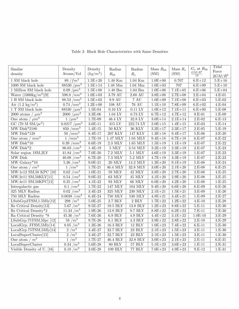
Table 2: Black Hole Characteristics with Same Densities

Similardensity

DensityAtoms/Vol

Density(kg/m3)

RadiusRbh

RadiusRs

Mass Rbh(SM)

Mass Rs(SM)

Gs at RbhGM/R2

10

TidalForce2GM/R3

1 SM black hole 89 /fm3 1.5E+20 1.48 Km 1.04 Km 1.0E+00 0.707 6.E+12 5.E+161000 SM black hole 88530 /pm3 1.5E+14 1.48 Mm 1.04 Mm 1.0E+03 707 6.E+09 5.E+101 Million SM black hole 0.09 /pm3 1.5E+08 1.48 Bm 1.04 Bm 1.0E+06 7.1E+05 6.E+06 5.E+04Water (1000kg/m3)[9] 598.8 /nm3 1.0E+03 3.79 AU 2.68 AU 3.8E+08 2.7E+08 2.E+04 4.E-011 B SM black hole 88.53 /nm3 1.5E+02 9.9 AU 7 AU 1.0E+09 7.1E+08 6.E+03 5.E-02Air (1.2 kg/m3) 0.74 /nm3 1.2E+00 108 AU 76 AU 1.1E+10 7.8E+09 6.E+02 4.E-041 T SM black hole 88530 /µm3 1.5E-04 0.16 LY 0.11 LY 1.0E+12 7.1E+11 6.E+00 5.E-082000 atoms / µm3 2000 /µm3 3.3E-06 1.04 LY 0.73 LY 6.7E+12 4.7E+12 9.E-01 1.E-09One atom / µm3 1 /µm3 1.7E-09 46.4 LY 32.8 LY 3.0E+14 2.1E+14 2.E-02 6.E-13GC (70 M SM/pc3) 0.0217 /µm3 3.6E-11 315 LY 222.74 LY 2.0E+15 1.4E+15 3.E-03 1.E-14MW Disk*2180 850 /mm3 1.4E-15 50 KLY 36 KLY 3.2E+17 2.3E+17 2.E-05 5.E-19MW Disk*128 50 /mm3 8.4E-17 207 KLY 147 KLY 1.3E+18 9.4E+17 5.E-06 3.E-20One atom / mm3 1 /mm3 1.7E-18 1.47 MLY 1.04 MLY 9.4E+18 6.7E+18 6.E-07 6.E-22MW Disk*10 0.39 /mm3 6.6E-19 2.3 MLY 1.65 MLY 1.5E+19 1.1E+19 4.E-07 2.E-22MW Disk*2 86.03 /cm3 1.4E-19 5 MLY 3.54 MLY 3.2E+19 2.3E+19 2.E-07 5.E-23Solar region 1SM,2LY 41.84 /cm3 7.0E-20 7.2 MLY 5.1 MLY 4.6E+19 3.3E+19 1.E-07 2.E-23MW Disk 40.08 /cm3 6.7E-20 7.3 MLY 5.2 MLY 4.7E+19 3.3E+19 1.E-07 2.E-23MW Galaxy*10 5.36 /cm3 9.0E-21 20 MLY 14.2 MLY 1.3E+20 9.1E+19 5.E-08 3.E-24One atom / cm3 1 /cm3 1.7E-21 46.4 MLY 32.8 MLY 3.0E+20 2.1E+20 2.E-08 6.E-25MW:1e12 SM,50 KPC [10] 0.62 /cm3 1.0E-21 59 MLY 42 MLY 3.8E+20 2.7E+20 2.E-08 4.E-25MW;2e11 SM,50KLY[11] 0.54 /cm3 9.0E-22 63 MLY 45 MLY 4.1E+20 2.9E+20 2.E-08 3.E-25MW;4e11 SM,50KPC[12] 0.25 /cm3 4.1E-22 93 MLY 66 MLY 6.0E+20 4.2E+20 1.E-08 1.E-25Intergalactic gas 0.1 /cm3 1.7E-22 147 MLY 104 MLY 9.4E+20 6.6E+20 6.E-09 6.E-26325 MLY Radius 0.02 /cm3 3.4E-23 325 MLY 230 MLY 2.1E+21 1.5E+21 3.E-09 1.E-26750 MLY Radius 0.0038 /cm3 6.4E-24 750 MLY 530 MLY 4.8E+21 3.4E+21 1.E-09 2.E-27LSubGrp3TSM,1.5Mly[12] 298 /m3 5.0E-25 2.7 BLY 2 BLY 1.7E+22 1.2E+22 4.E-10 2.E-28Rs Critical Density[13] 5.67 /m3 9.5E-27 19.5 BLY 13.8 BLY 1.2E+23 8.8E+22 5.E-11 3.E-30Rs Critical Density*2 11.34 /m3 1.9E-26 13.8 BLY 9.7 BLY 8.8E+22 6.2E+22 7.E-11 7.E-30Ra Critical Density *8 45.36 /m3 7.6E-26 6.9 BLY 4.9 BLY 4.4E+22 3.1E+22 1.0E-10 3.E-29LSubGrp.75TSM,Mpc [12] 58 /m3 9.7E-26 6.1 BLY 4.3 BLY 3.9E+22 2.8E+22 2.E-10 3.E-29LocalGrp; 3TSM,5Mly[14] 8.05 /m3 1.3E-26 16.3 BLY 12 BLY 1.0E+23 7.4E+22 6.E-11 5.E-30LocalGrp.75TSM,5Mly[14] 2 /m3 3.4E-27 32.7 BLY 23 BLY 2.1E+23 1.5E+23 3.E-11 1.E-30LocalSuperCluster[15] 2 /m3 3.4E-27 32.7 BLY 23 BLY 2.1E+23 1.5E+23 3.E-11 1.E-30One atom / m3 1 /m3 1.7E-27 46.4 BLY 32.8 BLY 3.0E+23 2.1E+23 2.E-11 6.E-31LocalSuperCluster 0.34 /m3 5.6E-28 80 BLY 57 BLY 5.1E+23 3.6E+23 1.E-11 2.E-31Visible Density of U. [16] 0.18 /m3 3.0E-28 109 BLY 77 BLY 7.0E+23 4.9E+23 9.E-12 1.E-31

4

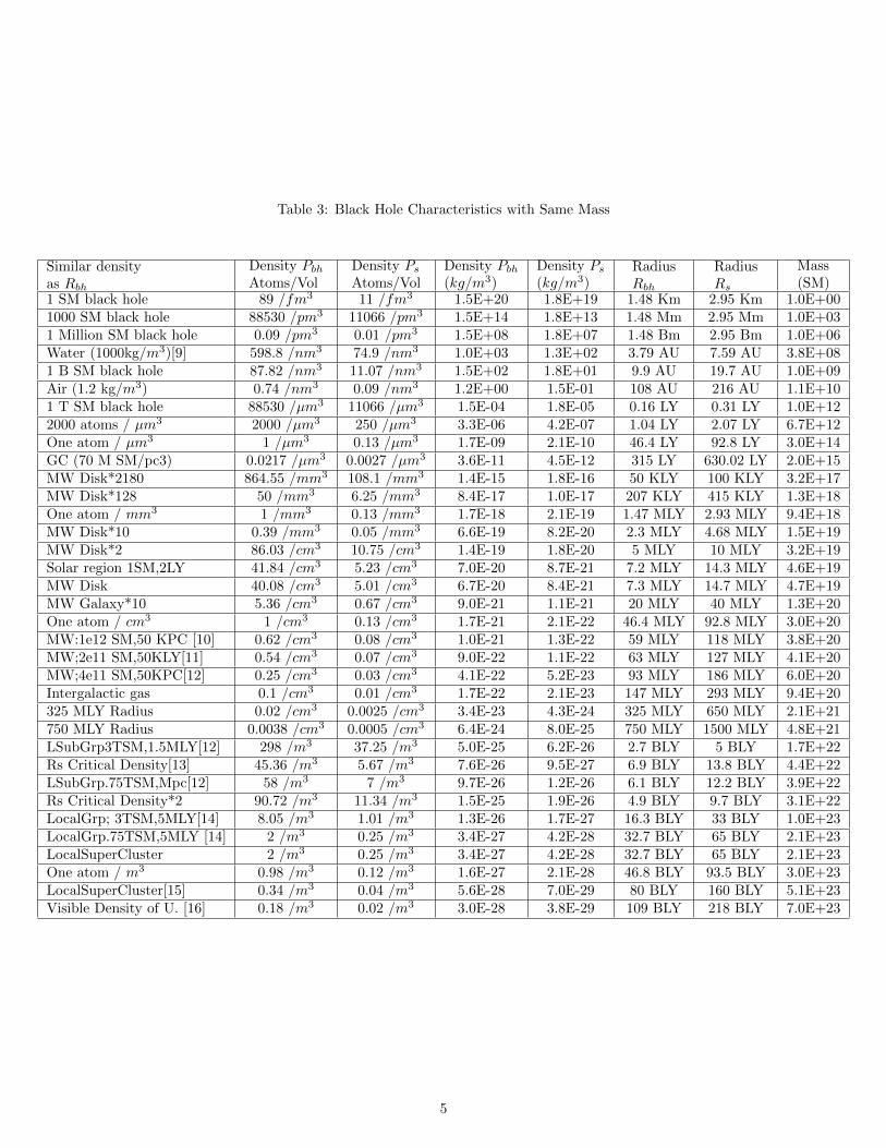
Table 3: Black Hole Characteristics with Same Mass

Similar densityas Rbh

Density PbhAtoms/Vol

Density PsAtoms/Vol

Density Pbh(kg/m3)

Density Ps(kg/m3)

RadiusRbh

RadiusRs

Mass(SM)

1 SM black hole 89 /fm3 11 /fm3 1.5E+20 1.8E+19 1.48 Km 2.95 Km 1.0E+001000 SM black hole 88530 /pm3 11066 /pm3 1.5E+14 1.8E+13 1.48 Mm 2.95 Mm 1.0E+031 Million SM black hole 0.09 /pm3 0.01 /pm3 1.5E+08 1.8E+07 1.48 Bm 2.95 Bm 1.0E+06Water (1000kg/m3)[9] 598.8 /nm3 74.9 /nm3 1.0E+03 1.3E+02 3.79 AU 7.59 AU 3.8E+081 B SM black hole 87.82 /nm3 11.07 /nm3 1.5E+02 1.8E+01 9.9 AU 19.7 AU 1.0E+09Air (1.2 kg/m3) 0.74 /nm3 0.09 /nm3 1.2E+00 1.5E-01 108 AU 216 AU 1.1E+101 T SM black hole 88530 /µm3 11066 /µm3 1.5E-04 1.8E-05 0.16 LY 0.31 LY 1.0E+122000 atoms / µm3 2000 /µm3 250 /µm3 3.3E-06 4.2E-07 1.04 LY 2.07 LY 6.7E+12One atom / µm3 1 /µm3 0.13 /µm3 1.7E-09 2.1E-10 46.4 LY 92.8 LY 3.0E+14GC (70 M SM/pc3) 0.0217 /µm3 0.0027 /µm3 3.6E-11 4.5E-12 315 LY 630.02 LY 2.0E+15MW Disk*2180 864.55 /mm3 108.1 /mm3 1.4E-15 1.8E-16 50 KLY 100 KLY 3.2E+17MW Disk*128 50 /mm3 6.25 /mm3 8.4E-17 1.0E-17 207 KLY 415 KLY 1.3E+18One atom / mm3 1 /mm3 0.13 /mm3 1.7E-18 2.1E-19 1.47 MLY 2.93 MLY 9.4E+18MW Disk*10 0.39 /mm3 0.05 /mm3 6.6E-19 8.2E-20 2.3 MLY 4.68 MLY 1.5E+19MW Disk*2 86.03 /cm3 10.75 /cm3 1.4E-19 1.8E-20 5 MLY 10 MLY 3.2E+19Solar region 1SM,2LY 41.84 /cm3 5.23 /cm3 7.0E-20 8.7E-21 7.2 MLY 14.3 MLY 4.6E+19MW Disk 40.08 /cm3 5.01 /cm3 6.7E-20 8.4E-21 7.3 MLY 14.7 MLY 4.7E+19MW Galaxy*10 5.36 /cm3 0.67 /cm3 9.0E-21 1.1E-21 20 MLY 40 MLY 1.3E+20One atom / cm3 1 /cm3 0.13 /cm3 1.7E-21 2.1E-22 46.4 MLY 92.8 MLY 3.0E+20MW:1e12 SM,50 KPC [10] 0.62 /cm3 0.08 /cm3 1.0E-21 1.3E-22 59 MLY 118 MLY 3.8E+20MW;2e11 SM,50KLY[11] 0.54 /cm3 0.07 /cm3 9.0E-22 1.1E-22 63 MLY 127 MLY 4.1E+20MW;4e11 SM,50KPC[12] 0.25 /cm3 0.03 /cm3 4.1E-22 5.2E-23 93 MLY 186 MLY 6.0E+20Intergalactic gas 0.1 /cm3 0.01 /cm3 1.7E-22 2.1E-23 147 MLY 293 MLY 9.4E+20325 MLY Radius 0.02 /cm3 0.0025 /cm3 3.4E-23 4.3E-24 325 MLY 650 MLY 2.1E+21750 MLY Radius 0.0038 /cm3 0.0005 /cm3 6.4E-24 8.0E-25 750 MLY 1500 MLY 4.8E+21LSubGrp3TSM,1.5MLY[12] 298 /m3 37.25 /m3 5.0E-25 6.2E-26 2.7 BLY 5 BLY 1.7E+22Rs Critical Density[13] 45.36 /m3 5.67 /m3 7.6E-26 9.5E-27 6.9 BLY 13.8 BLY 4.4E+22LSubGrp.75TSM,Mpc[12] 58 /m3 7 /m3 9.7E-26 1.2E-26 6.1 BLY 12.2 BLY 3.9E+22Rs Critical Density*2 90.72 /m3 11.34 /m3 1.5E-25 1.9E-26 4.9 BLY 9.7 BLY 3.1E+22LocalGrp; 3TSM,5MLY[14] 8.05 /m3 1.01 /m3 1.3E-26 1.7E-27 16.3 BLY 33 BLY 1.0E+23LocalGrp.75TSM,5MLY [14] 2 /m3 0.25 /m3 3.4E-27 4.2E-28 32.7 BLY 65 BLY 2.1E+23LocalSuperCluster 2 /m3 0.25 /m3 3.4E-27 4.2E-28 32.7 BLY 65 BLY 2.1E+23One atom / m3 0.98 /m3 0.12 /m3 1.6E-27 2.1E-28 46.8 BLY 93.5 BLY 3.0E+23LocalSuperCluster[15] 0.34 /m3 0.04 /m3 5.6E-28 7.0E-29 80 BLY 160 BLY 5.1E+23Visible Density of U. [16] 0.18 /m3 0.02 /m3 3.0E-28 3.8E-29 109 BLY 218 BLY 7.0E+23

5

Any G force, even the 3 trillion Gs would not be felt in free fall or while in orbit around the black hole.However, the tidal forces, the amount of dGs pulling on the center of the planet (or body) versus the outer sidecould rip one apart. Let ∆r be the distance between the center and the outer side. Tidal forces across an earthsize planet were computed using the following equation [18],

∆Gs(R) = Gs(R)−Gs(R+Rearth) = ±2GM∆r

R3(16)

where Rearth = ∆r = 6353000m. This table does not represent a new fundamental equation, but is just derivingRs and Rbh from density before computing the other parameters. Identical results can be found computing theequivalent density directly from the traditional black hole equations Rs = 2GM/C2 and Rbh = GM/C2. That is,given a mass M , compute Rs and Rbh, and then compute the Volume using V ol = 4/3πR3, then compute densityfrom P = M/V ol in kg/m3. In fact, Table 3 was computed in this fashion directly from the mass, and Table 2was derived from the mass densities, with identical results.

2.1 High Density Stellar Black Holes (R = 1.5∗103 - 3∗109m; M = 1 - 10MSM)

The data starts for a 1 SM stellar black hole (although in nature stellar black holes are believed to start at 2.8SMs). The mass density of the stellar black holes are listed at the top of Tables 2 and 3 with masses of 1, 1000, and1 million solar masses (SMs). Their densities are huge, because their large mass (e.g. 1 solar mass) is crammedinto very small radii (e.g 1.5 Km).

Note, that as the Mass increases by 1000 between the first three rows in Tables 2 and 3, the Radii also increaseby 1000, since both Rs and Rbh are proportional to M . The density values drop very quickly between these threerows (1 million fold with each 1000 increase in mass). Although their Mass increases 1000 fold, their radii alsoincrease 1000 fold, and their volume (not shown) increase 1 billion fold since volume is proportional to R3. Sincedensity = mass/volume; the 1000 fold increase in mass is over come by the 1 billion fold increase in volume,resulting in a million fold reduction in density. Thus, although the mass is increasing, the density decreases dueto its much larger volume.

The 1 SM black hole is very dense since it contains 1 solar mass in a very small 1.5km radius. It contains anequivalent mass of 11 to 89 hydrogen atoms in a cubic femtometer (fm = 1 ∗ 10−15 meters). Since the volume ofa neutron is about 1.76 fm3, the 1 SM finite black hole is 48 times denser than a neutron (or neutron star). TheRbh radius of a 1 K SM black hole would be 1500 km, which is just slightly smaller than the radius of the moon.The Rbh radius of a 1 M SM black hole would be 1.5 million km, which is about twice the size of the sun’s radius,but contains the mass of a million suns. Thus, stellar black holes are small and extremely dense.

For the 1 solar mass black hole, the G force is over 6 trillion Gs and its tidal force is 5 ∗ 1016dGs and wouldrip anything apart crossing the black hole boundary. However, the tidal force drops off quickly and is only 10 MdGs for the 1000 SM and 50,000 dGs for the 1 million SM stellar black holes. These high tidal dG forces aroundstellar black holes are believed to be the source of X-Ray emissions due to the high energy release of ripping apartatoms from material crossing the boundary of stellar black holes.

Possible candidates for stellar sized high density black holes, within the Milky Way includes Sagittarius A* aswell as smaller black holes believed to be within the globular clusters. Sagittarius A* is believed to be a 4 M SMblack hole within the core of the Milky Way Galaxy. Other Million SM black holes are reported in the cores ofother external galaxies.

2.2 Solar System Size Black Holes (R = 3.79 - 216AU ; M = 387M - 11BSM)

With a common density of water from Table 2, a Schwarzschild black hole would have a radius of 2.68 AU anda mass of 270 BSM (billion solar masses). A maximum spinning or charged black hole would have a radius of3.79 AU and a mass of 387 B SM. An Astronomical Unit (AU) is the orbital distance of the earth around the sunwhich is 1.496 ∗ 1011 meters. At 2.68 AU, the Schwarzschild radius would be out past twice the orbital radius ofMars around the sun and at 3.79 AU the spinning or charged black hole radius would be almost out to the orbitalradius of Jupiter around the sun. The G force drops to 20,000 Gs for the spinning or charged black hole and thetidal force drops to 0.4 dGs.

Using Table 3 the density of the 1 B SM finite black hole would be about 1/6th the density of water and beabout 10 AU in radius (just past the orbital radius of Saturn). The density of the 1 B SM Schwarzschild blackhole would be 1/50th the density of water and have Rs = 20 AU, and would extend out just past the orbitalradius of Uranus. The G force drops to 6000 Gs for the spinning or charged black hole and the tidal force dropsto 1/20th of a dG.

With the common density of air from Table 2, black holes would have Rs and Rbh radii of 76 and 108 AU,which are about 2 to 2.5 times the average orbital radius of Pluto around the sun and have masses of 7.8 B and11 B SM. The G force drops to 600 Gs and the tidal force is .0004 dGs.

Since the tidal forces of these solar system size black holes are not unreasonable, they may not emit x-rays.Possible candidates for solar system sized moderate density black holes are dark nebula gas clouds, the very centerof galactic cores, and quasars.

6

2.3 Light Year Size Black Holes (R = .16 to 100LY ; M = 1T to 300TSM)

Using Table 3 the trillion SM black holes, (i.e. million million), have Rbh and Rs radii of .16 and .31 LY and havedensities of 1.5 ∗ 10−4 kg/m3 to 1.8 ∗ 10−5kg/m3, which is 8,000-64,000 times less dense than air. The G force isjust 6 Gs and the tidal force has become .5 ∗ 10−9 (nano) dGs. Thus, one could orbit very close to this black holewithout being ripped apart.

With the common density of 2000 atoms per cubic micro meter (µm3) from Table 2, black holes would haveRs and Rbh radii of .7 and 1 LY, and have masses of about 4.7 and 6.7 T SM (which represents more mass thancurrent mass estimates for the entire Milky Way galaxy). The G force of this black hole would G = .9Gs, andthe tidal force would be a billionth dG.

With the common density of one atom per cubic micro meter (µm3) from Table 2, black holes would haveRs and Rbh radii of 33 and 46 LY, and have masses of about 200 and 300 T SM (which represents 200 to 300times the current mass estimates for the entire Milky Way galaxy). This seems impossible at first, but it is onlyequivalent to 1 hydrogen atom per cubic µm. One hydrogen atom per cubic micrometer would still be about 1billionth of the density of air and thus would not be out of the question. The G force of this black hole would be.02Gs, and the tidal force would be 6 ∗ 10−13dGs.

Possible candidates for light year sized low density black holes are dark nebula gas clouds, globular clusters(if they have additional dark matter), or the entire galactic core of a very large galaxy, (perhaps with additionaldark matter thrown in).

2.4 Galaxy Size Black Holes (R = 50K - 500KLY ; M = 3 ∗ 1017 - 3 ∗ 1018SM)

If the average density is equivalent to about 125 to 2180 times the density of the Milky Way disk, from Table3, the Rbh radii becomes 50K and 200K LY respectively. This would be small enough to just encompass mostgalaxies. From most galaxy speed curves, this seems improbable, unless the speed curves are only measuring themass of the galactic disk, and most of the mass is in the outer edges of the galaxy. The average density wouldonly be equivalent to 850 to 50 hydrogen atoms per cubic millimeters (mm3)

Candidate galaxy sized black holes are entire elliptical galaxies (but would need additional dark matter) .

2.5 Million Light Year Black Holes (R = 1M - 750MLY ; M = 9∗1018 - 5∗1021SM)

Tables 2 and 3 continue with mass densities producing MLY size black holes of larger, along with common densitiesseen in nature, that would need to be extended outward to fill the total volume to achieve the large total mass.

Note that the average mass density within these low density black holes includes the total mass of all the stars,dust, interstellar gas, and dark matter divided by their volumes. Consider our immediate solar region. The sun’sone solar mass divided by the volume of sphere with a radius of 2 LY would average about 40 hydrogen atomsper cubic cm, just counting the mass of the sun. The mass of the interstellar gas and the planets would be addedto this. If this solar region density was extended outward it would create a low density black holes in 5-7 M LYs.For this larger black hole, the average density includes the mass of its internal galaxies, including the total sumof its stars, galactic disk, and globular clusters, interstellar and intra-galactic gases, plus any hidden dark matter.

The mass density of the Milky Way Galactic disk is equivalent to about 40 hydrogen atoms/cm3 but can behigher in denser galaxies. Tables 2 and 3 include density entries corresponding to the mass density of the MilkyWay Galactic disk, and 2, 10,100, and 2000 times these values along with their corresponding characteristics.

The average density of the Milky Way Galaxy as a whole varies with estimates but is about .5 hydrogenatoms/cm3. If the average density of the Milky Way Galaxy is extended outward, this would make a low densityblack hole in 63 MLY. This would just be large enough to include the Local Supercluster. But its total masswould be 4 ∗ 1020 SM, which would be over 10,000 times the current mass estimate of the local Supercluster. Thisseems like an impossibly large mass, but it only averages out to be .5 hydrogen atoms per cubic cm.

Possible million light year black holes are the Local Supercluster and the Abell 1689 Galaxy cluster.

2.6 Billion Light Year Black Holes (R = 1B - 200BLY ; M = 4∗1022 - 5∗1023SM)

The mass density of the Milky Way Local Subgroup varies with estimates ranging between 58 to 300 hydrogenatoms/m3 depending on their total mass densities. If the local subgroup mass densities were extended outward,they would form a low density black hole in 2 to 6 BLYs.

The next rows in Tables 2 and 3 are related to the critical densities. Many scientists believe the average densityof the universe is near the critical density of 9.47∗10−27 kg/m3 which is equivalent to about 5.67 hydrogen atomsper cubic meter. The critical density is the density that would prevent the universe from expanding to infinity,even if the mass was traveling outward at the speed of light. This matches up precisely with the definition of alow density Schwarzschild black hole with radius Rs and using our equation comes out exactly to the 13.8 B LYradius. Thus, the Rs equation driving Tables 2 and 3 appear to match other calculations of critical density.

If one believes that the density of the universe is exactly at this value, they should realize that this wouldconstitute a large low density black hole, with the gravity trying to cancel the momentum from the big bang.

7

Using the Schwarzschild Classical black hole definition, it could still expand to infinity over all eternity beforestopping and reversing inward. And yes, if this were the case, by definition, we would be living in a SchwarzschildClassical low density black hole! Using the Schwarzschild Relativistic black hole definition, the edge would be anevent horizon and the expansion would stop immediately.

If the universe had exactly twice the critical density, equivalent to about 11.34 atoms of hydrogen per cubicmeter, and had the perceived 13.8 BLY radius, it would constitute a classical finite low density black hole. Ifthis were the case, the universe would begin to radically slow down and come to a stop within 200% Rbh heightwhich would be 27.6BLY. And yes, if this were the case, by definition, we would be living in a finite (relativistic)low density black hole. Using the relativistic spinning or charged black hole models, the edge would be an eventhorizon and the expansion would stop immediately.

The remaining entries of Tables 2 and 3 are for values that are less than the critical densities. Extending theestimated densities of the Local group results in Rbh = 12 to 23 BLYs and Rs = 16 to 33 BLYs. If the visibledensities of the Local Super cluster was extended outward, one would get a Rbh = 23 to 57 BLYs and Rs = 32 to80 BLYs. Using the density of 1 hydrogen atom per cubic meter results in Rbh = 32 BLYs and Rs = 46 BLYs.Using just the visible density of the universe puts the radius at Rbh = 77 BLYs and Rs = 109 BLYs. These radiiare all beyond the current estimated 13.8 BLY radius of the universe. If the universe has any of these densitiesless than the critical density, then the universe does not have to be inside a low density black hole.

If the expanding universe is below its critical mass and is almost a black hole, most matter traveling at lessthan the speed of light, would not escape. The light at the edge would get out, and not return, but the light fromlower orbits inside the black hole could still be curved inwards. Thus, we would still look like a low density blackhole, even before the universe collapsed completely into a black hole. If this were the case, we would not be livingin a low density black hole, but it may still look like we are.

Even if the complete universe is below its average critical mass density and not a low density black hole, typicalmodels of gravitational mass densities are denser in the center where we are presumed to be observing from. Thuswe could still be in a low density black hole, even if the entire universe is not a low density black hole.

A candidate billion light year sized black hole is the universe itself, or just portions including its center.

3 Candidate Localized Black Holes

Many astronomers believe black holes will be hard to detect or photograph because their internal light cannotescape the event horizon and all external light striking it would be sucked in and not reflected. Although a blackhole traps all internal light inside its event horizon, any interstellar gasses just outside the event horizon of astellar black hole should be ripped apart by the high tidal forces and cause X-Ray emissions. Thus, stellar blackholes should be easy to detect. Within the Milky Way Galaxy, X-Ray emissions have been detected inside globularclusters and at the galactic core. A 4 million solar mass black hole called Sagittarius A* is believed to be at thecore of the Milky Way Galaxy. We can’t quite see it since the Milky Way galactic disk obscures the view, but theorbits of objects have been plotted and the masses computed at 4MSM based on the orbit equations.

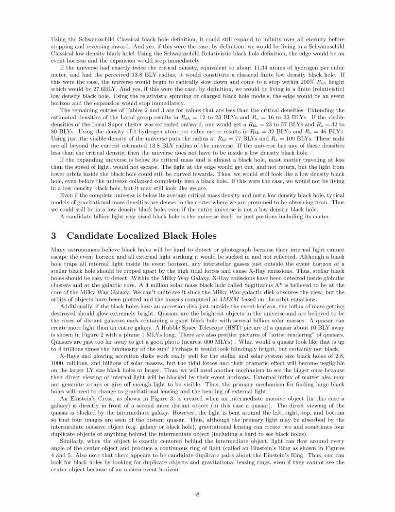
Additionally, if the black holes have an accretion disk just outside the event horizon, the influx of mass gettingdestroyed should glow extremely bright. Quasars are the brightest objects in the universe and are believed to bethe cores of distant galaxies each containing a giant black hole with several billion solar masses. A quasar cancreate more light than an entire galaxy. A Hubble Space Telescope (HST) picture of a quasar about 10 BLY awayis shown in Figure 2 with a plume 1 MLYs long. There are also prettier pictures of ”artist rendering” of quasars.Quasars are just too far away to get a good photo (nearest 600 MLYs) . What would a quasar look like that is upto 4 trillions times the luminosity of the sun? Perhaps it would look blindingly bright, but certainly not black.

X-Rays and glowing accretion disks work really well for the stellar and solar system size black holes of 2.8,1000, millions, and billions of solar masses, but the tidal forces and their dramatic effect will become negligibleon the larger LY size black holes or larger. Thus, we will need another mechanism to see the bigger ones becausetheir direct viewing of internal light will be blocked by their event horizons. External influx of matter also maynot generate x-rays or give off enough light to be visible. Thus, the primary mechanism for finding large blackholes will need to change to gravitational lensing and the bending of external light.

An Einstein’s Cross, as shown in Figure 3, is created when an intermediate massive object (in this case agalaxy) is directly in front of a second more distant object (in this case a quasar). The direct viewing of thequasar is blocked by the intermediate galaxy. However, the light is bent around the left, right, top, and bottomso that four images are seen of the distant quasar. Thus, although the primary light may be absorbed by theintermediate massive object (e.g. galaxy or black hole), gravitational lensing can create two and sometimes fourduplicate objects of anything behind the intermediate object (including a hard to see black holes).

Similarly, when the object is exactly centered behind the intermediate object, light can flow around everyangle of the center object and produce a continuous ring of light (called an Einstein’s Ring as shown in Figures4 and 5. Also note that there appears to be candidate duplicate pairs about the Einstein’s Ring. Thus, one canlook for black holes by looking for duplicate objects and gravitational lensing rings, even if they cannot see thecenter object because of an unseen event horizon.

8

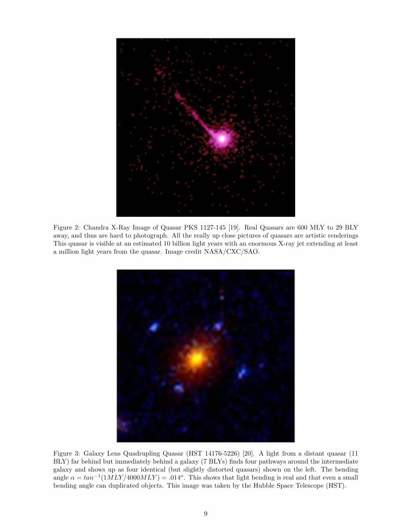
Figure 2: Chandra X-Ray Image of Quasar PKS 1127-145 [19]. Real Quasars are 600 MLY to 29 BLYaway, and thus are hard to photograph. All the really up close pictures of quasars are artistic renderingsThis quasar is visible at an estimated 10 billion light years with an enormous X-ray jet extending at leasta million light years from the quasar. Image credit NASA/CXC/SAO.

Figure 3: Galaxy Lens Quadrupling Quasar (HST 14176-5226) [20]. A light from a distant quasar (11BLY) far behind but immediately behind a galaxy (7 BLYs) finds four pathways around the intermediategalaxy and shows up as four identical (but slightly distorted quasars) shown on the left. The bendingangle α = tan−1(1MLY/4000MLY ) = .014o. This shows that light bending is real and that even a smallbending angle can duplicated objects. This image was taken by the Hubble Space Telescope (HST).

9

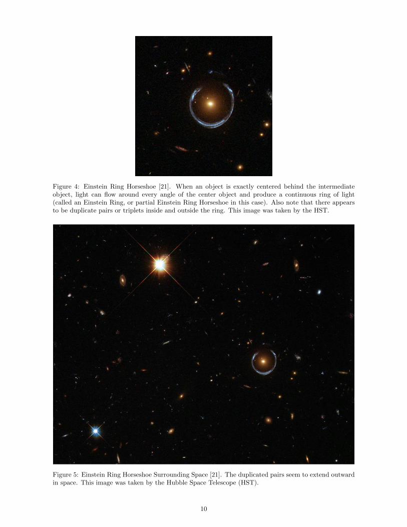
Figure 4: Einstein Ring Horseshoe [21]. When an object is exactly centered behind the intermediateobject, light can flow around every angle of the center object and produce a continuous ring of light(called an Einstein Ring, or partial Einstein Ring Horseshoe in this case). Also note that there appearsto be duplicate pairs or triplets inside and outside the ring. This image was taken by the HST.

Figure 5: Einstein Ring Horseshoe Surrounding Space [21]. The duplicated pairs seem to extend outwardin space. This image was taken by the Hubble Space Telescope (HST).

10

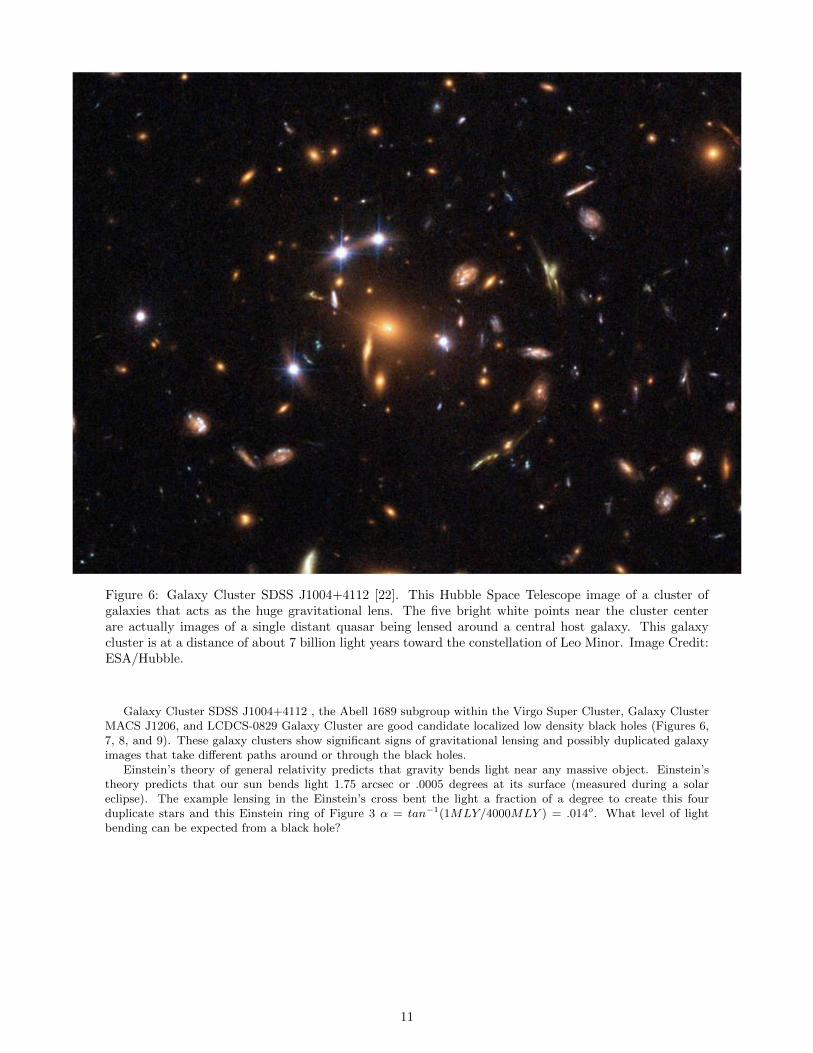
Figure 6: Galaxy Cluster SDSS J1004+4112 [22]. This Hubble Space Telescope image of a cluster ofgalaxies that acts as the huge gravitational lens. The five bright white points near the cluster centerare actually images of a single distant quasar being lensed around a central host galaxy. This galaxycluster is at a distance of about 7 billion light years toward the constellation of Leo Minor. Image Credit:ESA/Hubble.

Galaxy Cluster SDSS J1004+4112 , the Abell 1689 subgroup within the Virgo Super Cluster, Galaxy ClusterMACS J1206, and LCDCS-0829 Galaxy Cluster are good candidate localized low density black holes (Figures 6,7, 8, and 9). These galaxy clusters show significant signs of gravitational lensing and possibly duplicated galaxyimages that take different paths around or through the black holes.

Einstein’s theory of general relativity predicts that gravity bends light near any massive object. Einstein’stheory predicts that our sun bends light 1.75 arcsec or .0005 degrees at its surface (measured during a solareclipse). The example lensing in the Einstein’s cross bent the light a fraction of a degree to create this fourduplicate stars and this Einstein ring of Figure 3 α = tan−1(1MLY/4000MLY ) = .014o. What level of lightbending can be expected from a black hole?

11

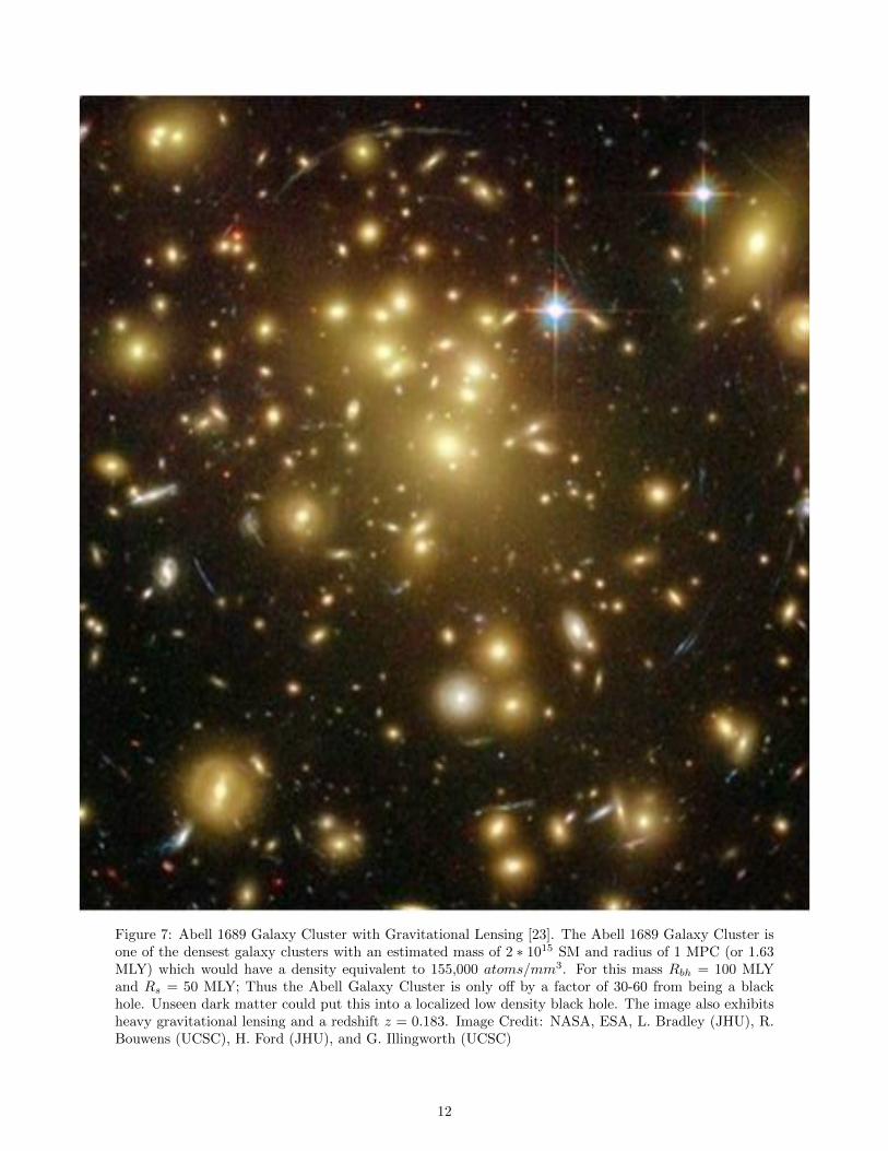
Figure 7: Abell 1689 Galaxy Cluster with Gravitational Lensing [23]. The Abell 1689 Galaxy Cluster isone of the densest galaxy clusters with an estimated mass of 2 ∗ 1015 SM and radius of 1 MPC (or 1.63MLY) which would have a density equivalent to 155,000 atoms/mm3. For this mass Rbh = 100 MLYand Rs = 50 MLY; Thus the Abell Galaxy Cluster is only off by a factor of 30-60 from being a blackhole. Unseen dark matter could put this into a localized low density black hole. The image also exhibitsheavy gravitational lensing and a redshift z = 0.183. Image Credit: NASA, ESA, L. Bradley (JHU), R.Bouwens (UCSC), H. Ford (JHU), and G. Illingworth (UCSC)

12

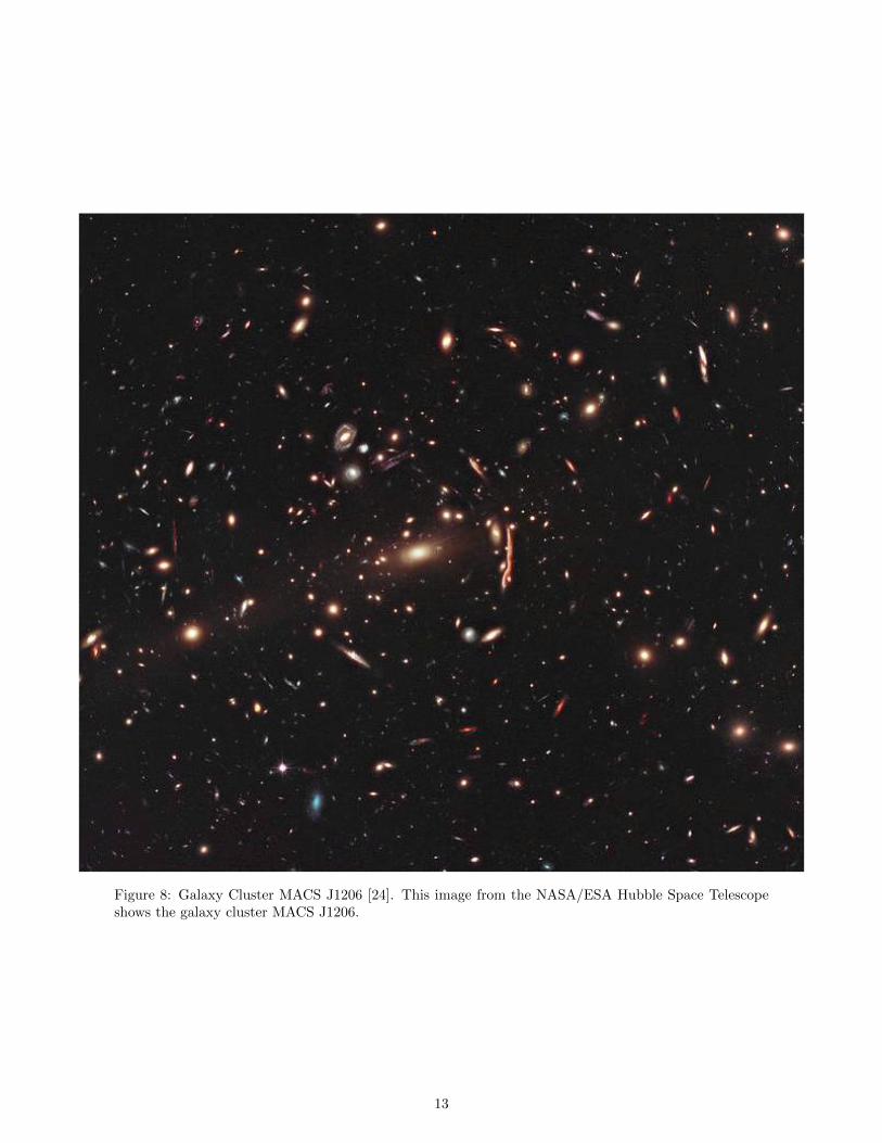
Figure 8: Galaxy Cluster MACS J1206 [24]. This image from the NASA/ESA Hubble Space Telescopeshows the galaxy cluster MACS J1206.

13

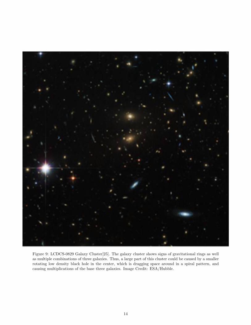
Figure 9: LCDCS-0829 Galaxy Cluster[25]. The galaxy cluster shows signs of gravitational rings as wellas multiple combinations of three galaxies. Thus, a large part of this cluster could be caused by a smallerrotating low density black hole in the center, which is dragging space around in a spiral pattern, andcausing multiplications of the base three galaxies. Image Credit: ESA/Hubble.

14

Einstein’s deflection angle, valid for small angles, isDa(R) = 4GM/(RC2) radians [26]. At 10Rs, a Schwarzschildblack hole can bend light roughly

Da(10Rs) =4GM

10(2GMC2

)C2

(17a)

= 0.2 radians = 11.5 degrees. (17b)

At 20Rbh, a spinning or charged black hole can bend light roughly

Da(20Rbh) =4GM

20(GMC2

)C2

(18a)

= 0.2 radians = 11.5 degrees. (18b)

Thus, light out to 10 ∗ Rs and 20 ∗ Rbh will bend light 11.5 degrees. This means that all stars, within 11.5degrees of 10 ∗ Rs and 20 ∗ Rbh will be duplicated. The primary star image will be seen directly (a little fartheraway from the black hole), and a duplicate image will appear on the far side of the black hole. For large blackholes, with a radius of 1 LY, 1000 LY, 1 million light years, 10 ∗Rs and 20 ∗Rbh could be quite large. In addition,light closer to the black hole just outside its photon sphere Rph would be bent up to 360 degrees as listed inSection 1 and computed in Appendix A. Thus, all stars farther out than 11.5 degrees will be duplicated on the farside of the black hole between Rph and Rbh ∗ 20. These duplicate images would appear like real stars or galaxyclusters. Thus, even relativistic black holes with a fully formed event horizon would appear like star or galaxyclusters from the outside because light from each external star or galaxy would be bent around the black hole andseen by the observer as an optical illusion duplicate star, galaxy, or cluster.

The following thought experiment may help. Hold up your thumb at arm’s length, and pick a distant object,say 5 to 10 degrees to the right. Pretend this distant object is an external galaxy, and your thumb is a black hole.You would see the external galaxy from the direct light on the right because the black hole is too far away todramatically affect its light path on the right. Now consider light from the object (external galaxy) heading to thefar left of the black hole (say 5 to 10 degrees left of your thumb). This light traveling to the left would also not bedramatically affected by the black hole and would head off towards the left unobserved. But now consider whathappens to the external galaxy’s light at decreasing angles from the left that is shining closer to the left of theblack hole. The light will start being bent towards the observer after passing by the black hole. The light will bebent slightly at first, and then more and more, up to a point where it will be bent 360 degrees and then collapseinto the black hole. But between these extremes, there exist an angle where the light will be bent exactly towardsyou (the observer), and the observer should see a duplicate galaxy just to the left of the black hole (thumb). Theduplicated galaxy will appear more distant than the original galaxy since the light had to travel farther (distanceto the black hole + distance from black hole to observer).

This same process will create a duplicate image illusion of every star or galaxy that is shining light on the blackhole. Since all external stars and galaxies shine light on the black hole, all stars and galaxies will be duplicated.All the duplicate images would appear around the black hole, as a cluster of stars or galaxies. Perhaps this maylook identical to the galaxy clusters of Figures 6, 7, 8, and 9.

If the mass is just short of the black hole definition, then the edge would not be a fully formed event horizonand light from inside could also be seen from the middle. Since each of these (nearly) black holes are probablyspinning to keep from collapsing, the light coming from within might take multiple paths through the core orpoles of the nearly black hole as it migrates outward. Due to frame dragging of the spinning mass could add aspiral pattern to the duplicated objects.

So what would a picture of a black hole possibly look like? Galactic cores like Sagittarius A*, Quasars, Globularclusters, galaxy clusters, and highly lensed galaxy clusters. Note that none of these black holes are really black,but are some of the brightest objects in the universe.

This of course is the view from the outside of a black hole. Section 8, 9, and 10 will discuss what it might lookfrom inside of a black hole.

15

4 Expanding Universe and Disproof of the Big Bang Theory

Is the expanding universe theory consistent with a universe which may be a black hole?

Theorem: An expanding universe isn’t consistent with Newton’s law of gravity.

Proof by Contradiction:Assume the following,

1. The universe is expanding

2. Newton’s law of gravity is valid through this expansion (or at least the latter portion of this expansion)

Following Newton’s law of gravity the black hole equations listed in Section 1 and derived in Appendix A are validthrough this expansion (or at least the latter portion of this expansion). Recall, these derivations only requiredcalculus and Newton’s law of gravity and Newton’s law of motion.

Consider the following three cases:

Case 1: Assume the current density of the universe with the current radius (Rcurrent) is at the critical density(Pcritical) and critical mass (Mcritical) such that it can be viewed as a Schwarzschild black hole. That is,

Pcritical =1.797 ∗ 10−6

R2current

kg/m3 (19)

Mcritical = Pcritical ∗ V = Pcritical ∗4π

3R3current (20)

Rcurrent =2GMcritical

C2(21)

Then it could be viewed as a low density black hole with Rs or Rcs = Rcurrent. Rcurrent is believed to be at 13.8BLY which would make Pcritical = 9.47 ∗ 10−27kg/m3. Using the Schwarzschild Relativistic black hole definition,the edge would be an event horizon and the expansion would stop immediately. Using the weaker SchwarzschildClassical black hole definition, it could still expand to infinity over all eternity before stopping and reversinginward.

Computing the finite (classical or smaller relativistic) black hole radius for the same mass (M = Mcritical) yields,

Rbh =GM

C2=

1

2

(2GM

C2

)=

1

2Rs =

1

2Rcurrent = 6.9 BLY. (22)

Note these black hole radii were also provided in Table 3. When the universe expanded through this Rbh valueof 6.9BLY in the past to get to Rcurrent, it would have been half the size, eight times denser, and would havebeen a finite black hole. If this was the case it would not have been able to double in size by definition of a finiteclassical black hole. Even mass traveling at the speed of light at the boundary of a finite classical black hole onlycan increase just up to 100% of its Rbh radius to get back to the current radius. But since no mass can travel atthe speed of light (other than light), the hard mass could not have been able to expand back to the current radius.Even light photons would be stopped at the photon sphere. Therefore the finite classical black hole (in the past)could not double its size to get to the current radius. This is a contradiction, so one of our assumptions must beinvalid! Thus, the universe cannot be exactly at the critical density in an expanding universe or the denser finiteblack hole in the past would have stopped the expansion.

A relativistic finite black hole (in the past) with Rbh = Rcurrent/2 would have had an event horizon atRcurrent/2 that would had stopped the expansion at Rcurrent/2.

Case 2: Assume the expanding universe is currently denser than the critical density Pcritical, then this wouldbe like the Schwarzschild black hole just discussed above at the exact critical mass density plus some extra massadded. In the past, at half its radius, it would be eight times denser, and be like the finite black hole at eight timesthe critical density, but with some extra mass added. Thus, the universe expansion would have been stopped bythis finite black hole, plus extra mass. Thus, that universe could not have doubled in radius to get to Rcurrent.This is a contradiction, so one of our assumptions must be invalid! Thus, the universe can’t be denser thanPcritical in an expanding universe.

Case 3: If one assume that the universe is expanding but is currently at a lesser density than the critical densityPcritical, that is Pcurrent = fPcritical where f < 1. Then we would not currently be in a low density black hole.However, in an expanding universe, the universe would have been much denser in the past and would still havebeen a finite black hole at a smaller radius.

16

To show this

M = Pcurrent4π

3R3current (23a)

= fPcritical4π

3R3current (23b)

= fMcritical (23c)

Let M = fMcritical, where f < 1 is the lesser (fractional mass) such that P = fPs and Mcritical is the massdensity of the critical universe above. Then

Rbh =GM

C2(24a)

=1

2

(2GM

C2

)(24b)

=1

2

(2GfMcritical

C2

)(24c)

=1

2fRcurrent (24d)

= 6.9f BLY. (24e)

Since f is less than 1, the universe would have been in a finite relativistic black hole prior to 6.9 BLY, which wouldhave prevented it from more than doubling in size to 13.8 BLY.

For example, if one assumes a density of one hydrogen atom per cubic meter (1.67 ∗ 10−27kg/m3); f =1.678 ∗ 10−27/(9.47 ∗ 10−27) = 1/5.67; Rbh = 1/5.67 ∗ 6.9 BLY = 1.22 BLY. But if the lesser dense universe was afinite black hole at a smaller size f ∗ 6.9 BLY (e.g. 1.22 BLY), it would not have expanded greater than 100% ofthis size (e.g. 2.44 BLY) to get to its current size of 13.8 BLY. This is a contradiction, so one of our assumptionsmust be invalid! Thus, the universe cannot be at less than the critical density in an expanding universe.

Since all possible densities were covered in the above three cases, in an expanding universe and encounteredcontradictions with each one, the invalid assumption must be that the universe is an expanding universe. There-fore the expanding universe theory is inconsistent with Newton’s law of gravity.

Thus, the expanding universe theory from the big bang is invalid because the smaller denser universe in thepast would have constituted a finite (classical or relativistic) black hole that would have stopped its expansion.

Thus, we are not in an expanding universe, and probably never were in an expanding universe, and the bigbang probably did not happen. The Doppler redshift originally associated with expanding universe will need tobe replaced with another mechanism. Possible candidates are translational redshift, gravitational redshift, andintrinsic redshift mechanisms, or a combination. These will be covered in Section 7.

The only possible way I see to preserve an expanding universe due to the big bang, is to suspend Newton’slaw of gravity in its earlier phases (perhaps the expansion phase), until the universe got past its finite black holeradius (Rbh) or fractional Rbh (1.25-6.9 BLY). This would bypass the contradiction found in the analysis above.That is, declare F = GmM/R2 invalid for up to half of the expansion. But ideally, physical theories should beself consistent and not require the suspension of the laws of physics.

Physicists had to suspend the laws of physics during the initial seconds of the explosion until each fragmentwas less dense than a black hole. They also envisioned some fragments were micro black holes and perhaps stellarblack holes, that now may be contributing to dark matter. However they failed to realize that the collection ofall fragments also constituted a relativistic large low density black hole, out until it passes one half its criticaldensity radius or fractional radius (e.g. 1.22BLY to 6.9 BLY).

Some physicists have also introduced the concept of dark energy to try to add a 10 to 25% correction neededto match an expanding universe that is perceived as expanding even faster over time. This basically adds anunknown repulsive force to override or counteract the gravitational force, F = GmM/R2.

This dark energy force would also have to be able to keep the finite black hole from collapsing when theexpanding universe was a half, quarter, and eighth its current radius, when it was 8, 64, and 512 times denser.Thus, the dark energy repulsive force would also have to scale with size. However, I believe one should firstexplore all the alternatives offered by the simpler gravity equation above before tweaking constants, adding terms,or adding new (unseen) physical concepts, especially if it is pretty clear that the universe is not expanding. Thisexploration process of the remaining alternatives is the goal of the rest of this paper.

17

5 Non-Expanding Universe Options

If we are not in an expanding universe, other options include: 1) an infinite universe 2) collapsing universe, 3)non-expanding or slowly collapsing universe, 4) a reflecting universe or 5) an oscillating universe.

5.1 Infinite Universe

If the universe is infinite, with finite density, however small, we would be in a low density black hole since themass would extend to a finite black hole radius corresponding to that density. Thus, infinite space would collapseinto disjoint low density black holes. If the universe is infinite we would probably be in one of the disjoint lowdensity black holes. Even if we were ”lucky” and within a lagrange point exactly between two disjoint low densityblack holes, the collection of nearby disjoint low density black holes including ourselves would still constitute alarger low density black hole. Thus, if the universe was infinite, we would be in a low density black hole.

An infinite universe made of disjoint low density black holes escapes Olber’s paradox [27] of being infinitelybright with its infinite lights since the light available within each black hole would be finite. Thus, if we are inan infinite universe of disjoint low density black holes, the universe could look finite because the infinite externallight is trapped in external black holes.

If this is the case, the infinite universe would be lying to us by cloaking itself in an infinite number of invisibleevent horizons. However, since we would be inside a localized black hole, the internal light from our localizedblack hole would be ”reflected” backwards by our event horizon, and create the illusion (second lie) that weare in an infinite universe (see reflective universe subsection below). But, if this is the case, the second lie wouldactually cancel the first lie and accidentally convey the truth, that we would be actually within an infinite universe.Unfortunately, if we are trapped within a localized black hole, we may never know. If we are in an infinite universeof an infinite number of black holes, but no one can see their light, are they really there?

If we are in an infinite universe and other lagrange galaxies exist just outside our localized black hole, wemay be able to still see them, but they may not be able to see us. That is, they may not be able to see internallight from our black hole. External galaxies may only be able to see our gravitational lensing effect and we wouldappear like a galaxy cluster, perhaps of the lucky ”galaxies” at the lagrange points. Similarly, external black holesmay only be visible as galaxy clusters of lagrange galaxies. But these may be overwhelmed by the reflections ofinternal galaxies.

5.2 Rapidly Collapsing Universe

If we were in a finite collapsing universe denser than Pcritical, we would be in a low density black hole. Collapsinginto a black hole would be the expected natural process. However, if the universe was rapidly collapsing, onewould see a blue shift which is currently not observed, (and we would be crushed by now). Thus, the universe isnot rapidly collapsing.

However, the light from the edge of the universe may be up to 13.8 BLY old, and thus, all that we know isthat the universe was not rapidly collapsing 13.8 B years ago. Since that time, it could have begun collapsingvery rapidly. For example, 10 billion years ago it could have started to collapse and we wont find out until about4 billion years from now. But as of this time, we have no evidence that we are rapidly collapsing.

There are also very bright quasars being detected at large distances that are heavily redshifted. This redshiftwould argue against a collapsing universe. However, as we will see in Section 7, the quasar redshift could be causedby gravitational redshift, which could override a smaller blueshift due to a collapsing universe. Additionally, thecollapsing mass at the edge of the universe into the quasar would explain why there are no nearby quasars. Thus,the quasars redshift could also be supporting evidence for a collapsing universe as well.

5.3 Non-expanding or Slowly Collapsing Universe

If the universe was less dense than Pcritical and in a non-expanding or slowly collapsing universe, we would notbe in a low density black hole, yet, until the universe collapses and its density increases to Pcritical. Note: lightcould still get out, but the mass would continue to collapse. But after it collapses to Pcritical, then even lightwould no longer be able to escape. Thus, if we are not in a low density black hole, we will eventually be in one.

Additionally, most conventional models of gravitational mass densities have higher densities in the center(where we would be observing from). Thus, we could still be in a low density black hole, even if the entireuniverse has not yet collapsed into a low density black hole. Thus, we are probably living in a low density blackhole, or eventually will be.

Note that a non-expanding or slowly collapsing universe would be the closest model to the existing expandinguniverse model. The universe could even be the same size, but just need to replace the Doppler redshift explanationwith an alternate mechanism. The universe could be finite and non-reflecting.

18

5.4 Reflecting Universe

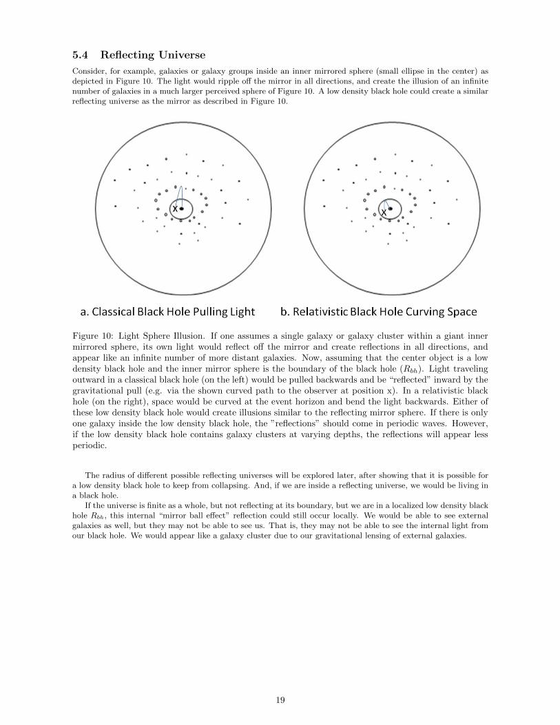
Consider, for example, galaxies or galaxy groups inside an inner mirrored sphere (small ellipse in the center) asdepicted in Figure 10. The light would ripple off the mirror in all directions, and create the illusion of an infinitenumber of galaxies in a much larger perceived sphere of Figure 10. A low density black hole could create a similarreflecting universe as the mirror as described in Figure 10.

Figure 10: Light Sphere Illusion. If one assumes a single galaxy or galaxy cluster within a giant innermirrored sphere, its own light would reflect off the mirror and create reflections in all directions, andappear like an infinite number of more distant galaxies. Now, assuming that the center object is a lowdensity black hole and the inner mirror sphere is the boundary of the black hole (Rbh). Light travelingoutward in a classical black hole (on the left) would be pulled backwards and be “reflected” inward by thegravitational pull (e.g. via the shown curved path to the observer at position x). In a relativistic blackhole (on the right), space would be curved at the event horizon and bend the light backwards. Either ofthese low density black hole would create illusions similar to the reflecting mirror sphere. If there is onlyone galaxy inside the low density black hole, the ”reflections” should come in periodic waves. However,if the low density black hole contains galaxy clusters at varying depths, the reflections will appear lessperiodic.

The radius of different possible reflecting universes will be explored later, after showing that it is possible fora low density black hole to keep from collapsing. And, if we are inside a reflecting universe, we would be living ina black hole.

If the universe is finite as a whole, but not reflecting at its boundary, but we are in a localized low density blackhole Rbh, this internal “mirror ball effect” reflection could still occur locally. We would be able to see externalgalaxies as well, but they may not be able to see us. That is, they may not be able to see the internal light fromour black hole. We would appear like a galaxy cluster due to our gravitational lensing of external galaxies.

19

5.5 Oscillating Universe

The oscillating universe, in the literature, generally comes from having the expanding universe eventually collapse,into a singularity, where there may be a subsequent explosion (subsequent big bang) and cause a subsequentexpansion phase, thus repeating the process. But this would run into the similar problems of the expandinguniverse, which requires breaking Newton’s law of gravity. Thus, oscillating universes in literature that dependon an expanding universe would not occur.

5.5.1 Active Objects

Another possible source for oscillation through temporary expansion is the active plumes of neutron stars, blackholes, and quasars. Recall, that the black hole escape velocity equations were for inert, ballistic projectiles. Activeobjects with active plumes are more like relativistic rockets that could expand one outward against the forces ofgravity. If an active object is within an event horizon of a black hole with a negligible G force (e.g. less than anano G), then an active object may be able to escape the event horizon.

5.5.2 Diminished Gravity

Another possible source for oscillation through temporary expansion would be if gravitational waves from insidethe black hole were affected by the collapse of space around the black hole. That is, as mass collapses into a blackhole, where nothing can escape or be seen externally, not even light nor other electromagnetic waves; its owninternal gravitational waves might also become blocked and not escape, or at least be diminished. The light fromexternal objects could still get in, thus gravity waves from external objects should still be felt, but the reversemay not be true. However, this seems like it would break the principle of physics: for every action there is anequal and opposite reaction. Thus, this seems implausible.

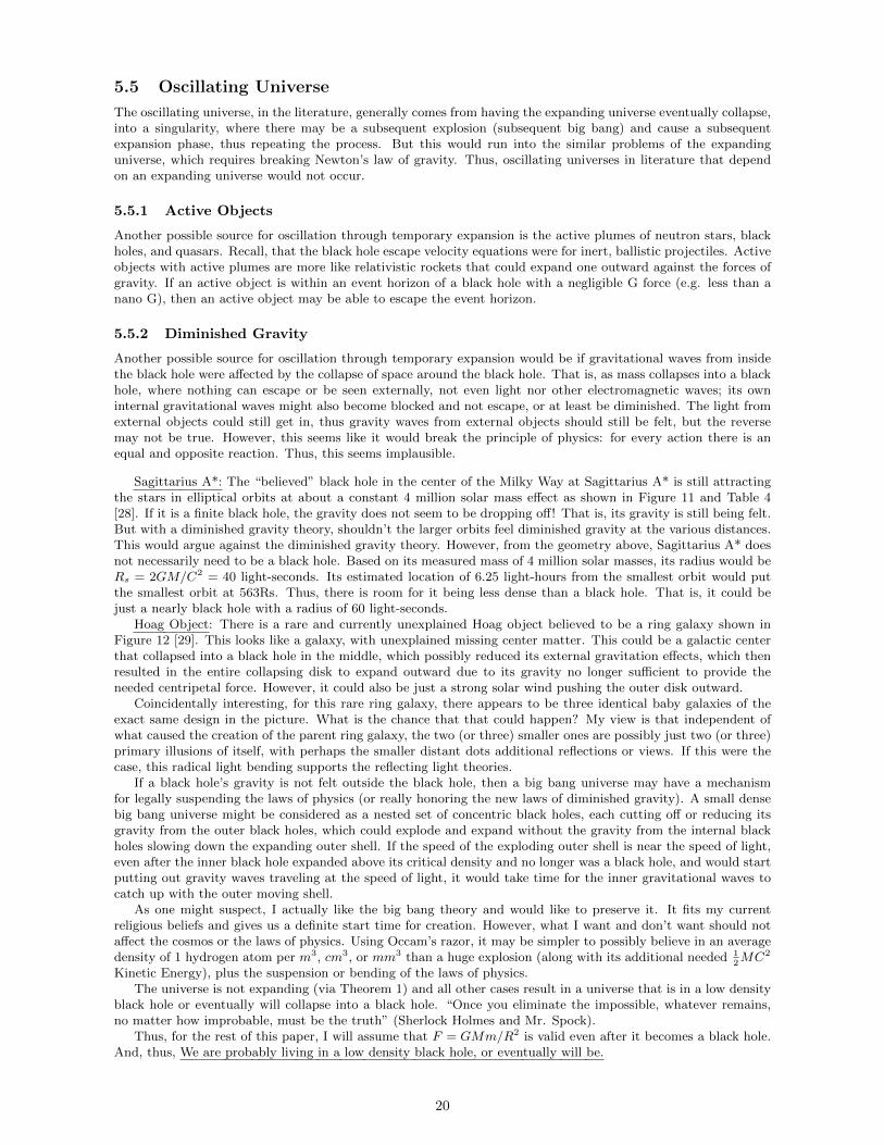
Sagittarius A*: The “believed” black hole in the center of the Milky Way at Sagittarius A* is still attractingthe stars in elliptical orbits at about a constant 4 million solar mass effect as shown in Figure 11 and Table 4[28]. If it is a finite black hole, the gravity does not seem to be dropping off! That is, its gravity is still being felt.But with a diminished gravity theory, shouldn’t the larger orbits feel diminished gravity at the various distances.This would argue against the diminished gravity theory. However, from the geometry above, Sagittarius A* doesnot necessarily need to be a black hole. Based on its measured mass of 4 million solar masses, its radius would beRs = 2GM/C2 = 40 light-seconds. Its estimated location of 6.25 light-hours from the smallest orbit would putthe smallest orbit at 563Rs. Thus, there is room for it being less dense than a black hole. That is, it could bejust a nearly black hole with a radius of 60 light-seconds.

Hoag Object: There is a rare and currently unexplained Hoag object believed to be a ring galaxy shown inFigure 12 [29]. This looks like a galaxy, with unexplained missing center matter. This could be a galactic centerthat collapsed into a black hole in the middle, which possibly reduced its external gravitation effects, which thenresulted in the entire collapsing disk to expand outward due to its gravity no longer sufficient to provide theneeded centripetal force. However, it could also be just a strong solar wind pushing the outer disk outward.

Coincidentally interesting, for this rare ring galaxy, there appears to be three identical baby galaxies of theexact same design in the picture. What is the chance that that could happen? My view is that independent ofwhat caused the creation of the parent ring galaxy, the two (or three) smaller ones are possibly just two (or three)primary illusions of itself, with perhaps the smaller distant dots additional reflections or views. If this were thecase, this radical light bending supports the reflecting light theories.

If a black hole’s gravity is not felt outside the black hole, then a big bang universe may have a mechanismfor legally suspending the laws of physics (or really honoring the new laws of diminished gravity). A small densebig bang universe might be considered as a nested set of concentric black holes, each cutting off or reducing itsgravity from the outer black holes, which could explode and expand without the gravity from the internal blackholes slowing down the expanding outer shell. If the speed of the exploding outer shell is near the speed of light,even after the inner black hole expanded above its critical density and no longer was a black hole, and would startputting out gravity waves traveling at the speed of light, it would take time for the inner gravitational waves tocatch up with the outer moving shell.

As one might suspect, I actually like the big bang theory and would like to preserve it. It fits my currentreligious beliefs and gives us a definite start time for creation. However, what I want and don’t want should notaffect the cosmos or the laws of physics. Using Occam’s razor, it may be simpler to possibly believe in an averagedensity of 1 hydrogen atom per m3, cm3, or mm3 than a huge explosion (along with its additional needed 1

2MC2

Kinetic Energy), plus the suspension or bending of the laws of physics.The universe is not expanding (via Theorem 1) and all other cases result in a universe that is in a low density

black hole or eventually will collapse into a black hole. “Once you eliminate the impossible, whatever remains,no matter how improbable, must be the truth” (Sherlock Holmes and Mr. Spock).

Thus, for the rest of this paper, I will assume that F = GMm/R2 is valid even after it becomes a black hole.And, thus, We are probably living in a low density black hole, or eventually will be.

20

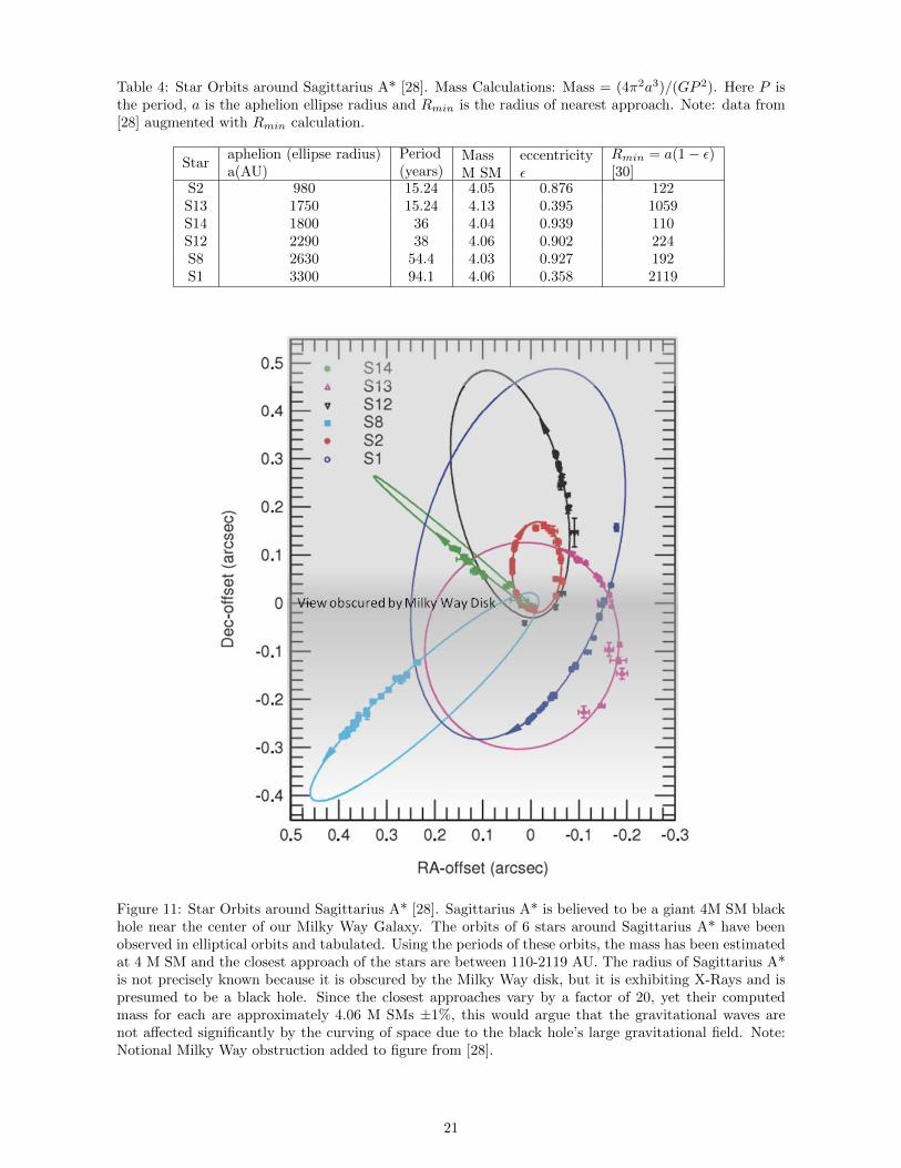
Table 4: Star Orbits around Sagittarius A* [28]. Mass Calculations: Mass = (4π2a3)/(GP 2). Here P isthe period, a is the aphelion ellipse radius and Rmin is the radius of nearest approach. Note: data from[28] augmented with Rmin calculation.

Staraphelion (ellipse radius)a(AU)

Period(years)

MassM SM

eccentricityε

Rmin = a(1− ε)[30]

S2 980 15.24 4.05 0.876 122S13 1750 15.24 4.13 0.395 1059S14 1800 36 4.04 0.939 110S12 2290 38 4.06 0.902 224S8 2630 54.4 4.03 0.927 192S1 3300 94.1 4.06 0.358 2119

Figure 11: Star Orbits around Sagittarius A* [28]. Sagittarius A* is believed to be a giant 4M SM blackhole near the center of our Milky Way Galaxy. The orbits of 6 stars around Sagittarius A* have beenobserved in elliptical orbits and tabulated. Using the periods of these orbits, the mass has been estimatedat 4 M SM and the closest approach of the stars are between 110-2119 AU. The radius of Sagittarius A*is not precisely known because it is obscured by the Milky Way disk, but it is exhibiting X-Rays and ispresumed to be a black hole. Since the closest approaches vary by a factor of 20, yet their computedmass for each are approximately 4.06 M SMs ±1%, this would argue that the gravitational waves arenot affected significantly by the curving of space due to the black hole’s large gravitational field. Note:Notional Milky Way obstruction added to figure from [28].

21

Figure 12: Hoag Ring Galaxy [29]. This Hoag Ring Galaxy appears to be missing its internal mass. Ifthe center has become a low density black hole, where no light or electromagnetic radiation can escape,maybe some of its gravitational waves are also affected (diminished) and are no longer able to hold inthe galactic disk. If this was the case, the centripetal force needed by stars orbiting the center would nolonger be provided by the central gravitational force, and all stars would fly outward, possibly producingthe observed Hoag Ring Galaxy. Alternately, there could just be a strong intergalactic solar wind comingfrom the core. Coincidentally, note the two baby Hoag like objects in the background and possibly morein the distance. Since the Hoag object is not a common phenomena, it is unlikely that there would bethree (or more) in such a close proximity. Thus, these miniature Hoag objects may be gravitationalreflections from a low density black hole caused by the core of the Hoag Ring Galaxy. Image Credit:NASA and The Hubble Heritage Team (STScI/AURA) Acknowledgment: Ray A. Lucas (STScI/AURA)

The source of the initial hydrogen or dust is still an unanswered question. It could have been created as a giantinitial hydrogen or dust cloud or be continually formed incrementally (by a Creator or one of the steady statetheory mechanisms or quantum mechanics creating something out of nothingness). However, if it was always justthere, it should have already collapsed earlier. Thus, what has been presented so far has not ruled out the needfor the dust (hydrogen), nor ruled out the beginning of time. The exact date of the beginning, however, based onthe big bang and Doppler redshift is no longer necessarily 13.8 billion years. We will also need new mechanismsfor the redshift and a mechanism to keep it from collapsing.

22

6 Non-collapsing Black Hole via Rotation

Black holes are assumed to collapse very quickly to a singularity, since no force seems available to counteract itsstrong gravitation forces. However, simple centripetal force increases with the square of the velocity and can growto balance the gravitational forces. The conservation of angular momentum would also encourage this to happen.The mass just needs to be orbiting fast enough to cancel the gravitational forces. Setting the centripetal force(Fcent) equal to the gravitational force at any radius within the black hole, one can compute the orbiting velocity,V , to effectively cancel its gravitational force (Fgrav) [31].

Fgrav =GmM

R2= Fcent =

mV 2

R(25)

V 2 =GM

R(26)

6.1 At the surface (with radii Rs and Rbh)

Let V = Vs denote the velocity for an object orbiting at the surface.

For a Schwarzschild black hole, using Equation 26 becomes:

V 2s =

GM

Rs=

GM

(2GM/C2)=C2

2(27)

Vs =C√

2= .707C (28)

For an Rbh black hole:

V 2s =

GM

Rbh=

GM

(GM/C2)= C2 (29)

Vs = C (30)

One might think this is a mistake, since nothing can travel as fast as the speed of light C, and everything travelingless than the speed of light would be pulled in and even light would not be able to escape but be locked in acircular orbit. But this is exactly the black hole effect we were expecting. Thus, the outer velocities of .707C andC look OK.

It may also seem impossible to get mass traveling at the speed of light. But even with the classical finite(twice) height black hole, any mass dropped at 2 ∗ Rbh would be traveling at or near the speed of light by timeit hit Rbh. It is just the return velocity profile of throwing up a rock at initial velocity C from the surface ofthe finite (twice) height black hole. The rock would start out at velocity C, but slow down and stop at the topwhere R = 2 ∗Rbh, then it would fall backward and impact the surface back at its initial velocity C. Thus, simplydropping a rock at R = 2∗Rbh would also be traveling at velocity C when it reached the surface of the black hole.

6.2 Within the finite black hole at radius R

Here we consider various mass density functions P (R) and compute their mass function M(R) and needed velocityfunctions V (R) to keep the black hole from collapsing.

6.2.1 P (R) that is inversely proportional to R2

First, assume a Kepler mass density function P (R) that is inversely proportional to R2. This is typically seenwithin solar systems. That is

P (R) =K

R2(31)

where K is chosen in order to produce the same overall mass M of the black hole. Since density depends on radius,mass is also a function of the radius. Consider M(R), the mass of a sphere with radius R. This mass can beexpressed using the spherical shell method with density P (R) and surface area 4πR2,

M(R) =

∫ R

0

P (r)4πr2dr (32)

=

∫ R

0

K

r24πr2dr (33)

=

∫ R

0

K4πdr (34)

= 4πKR (35)

23

K is a constant chosen so that total mass M = M(Rbh) is equal to the average density Pavg times its total volumeV ol = 4π

3R3bh. We use these in order to solve for an expression for K,

M = M(Rbh) = 4πKRbh = Pavg ∗ (4π

3R3bh) (36)

K =1

3PavgR

2bh (37)

Plugging K into our expression for M(R) from Eq. 35 yields

M(R) = 4π ∗ (1

3PavgR

2bh) ∗R (38)

= Pavg ∗4π

3R3bh

(R

Rbh

)(39)

= M ∗(R

Rbh

)(40)

Then the orbital velocity at radius R, V (R) can be derived using Eq. 26 and Rbh = GMC2 .

V (R)2 =G ∗M(R)

R(41)

=G ∗ (M ∗ ( R

Rbh))

R(42)

=GM

Rbh(43)

= C2 (44)

thereforeV (R) = C (45)

Thus the velocity V is a constant independent of R. Therefore, an object has to maintain the speed of light at allradii to keep from falling inward. Thus, anything going less than the speed of light will collapse into the center.Thus, any black hole with a Kepler distribution inversely proportional to R2 will collapse, just like one sees in themovies.

6.2.2 P (R) that is inversely proportional to R

Now assume a mass density function P (R) that is inversely proportional to R. This is typically seen withinGalactic disks. That is

P (R) =K

R(46)

where K is chosen in order to produce the same overall mass M of the black hole. Since density depends on radius,mass is also a function of the radius. Consider M(R), the mass of a sphere with radius R. This mass can beexpressed using the spherical shell method with density P (R) and surface area 4πR2,

M(R) =

∫ R

0

P (r)4πr2dr (47)

=

∫ R

0

K

r4πr2dr (48)

=

∫ R

0

K4πrdr (49)

= 2πKR2 (50)

K is a constant chosen so that total mass M = M(Rbh) is equal to the average density Pavg times its total volumeV ol = 4π

3R3bh. We use these in order to solve for an expression for K,

M = M(Rbh) = 2πKR2bh = Pavg ∗ (

4π

3∗R3

bh) (51)

K =2

3PavgRbh (52)

Plugging K into our expression for M(R) (Eq. 50) yields

24

M(R) = 2π(2

3PavgRbh)R2 (53)

= Pavg ∗4π

3R3bh

(R2

R2bh

)(54)

= M ∗(R

Rbh

)2

(55)

Then the orbital velocity at radius R, V (R) can be derived using Eq. 26 and and Rbh = GMC2 .

V (R)2 =G ∗M(R)

R(56)

V (R)2 =G ∗ (M ∗

(RRbh

)2)

R(57)

=GM

Rbh∗ R

Rbh(58)

= C2 ∗ R

Rbh(59)

therefore

V (R) =C√Rbh

√R (60)

Thus V (R) is proportional to√R.

V (R) = C

√R

Rbh(61)

At the surface, R = Rbh, velocity is the speed of light V = C. As one moves inwards the fractional radius ( RRbh

)decreases and approaches zero. The velocity is proportional to the square root of this fractional radius. Thus theblack hole with mass distribution inverse proportional to R does not need to collapse.

6.2.3 P (R) that is a constant

Now assume a mass density function P (R) that is constant. That is

P (R) = K (62)

where K is chosen in order to produce the same overall mass M of the black hole. Consider M(R), the mass of asphere with radius R. This mass can be expressed using the spherical shell method with density P (R) and surfacearea 4πR2,

M(R) =

∫ R

0

P (r)4πr2dr (63)

=

∫ R

0

K4πr2dr (64)

=4π

3KR3 (65)

K is a constant chosen so that total mass M = M(Rbh) is equal to the average density Pavg times its total volumeV ol = 4π

3R3bh. We use these in order to solve for an expression for K,

M = M(Rbh) =4π

3KR3

bh = Pavg ∗ (4π

3R3bh) (66)

K = Pavg (67)

Plugging K into our expression for M(R) (Eq. 65) yields

M(R) =4π

3PavgR

3 (68)

= Pavg ∗4π

3R3bh

(R3

R3bh

)(69)

= M ∗(R

Rbh

)3

(70)

25

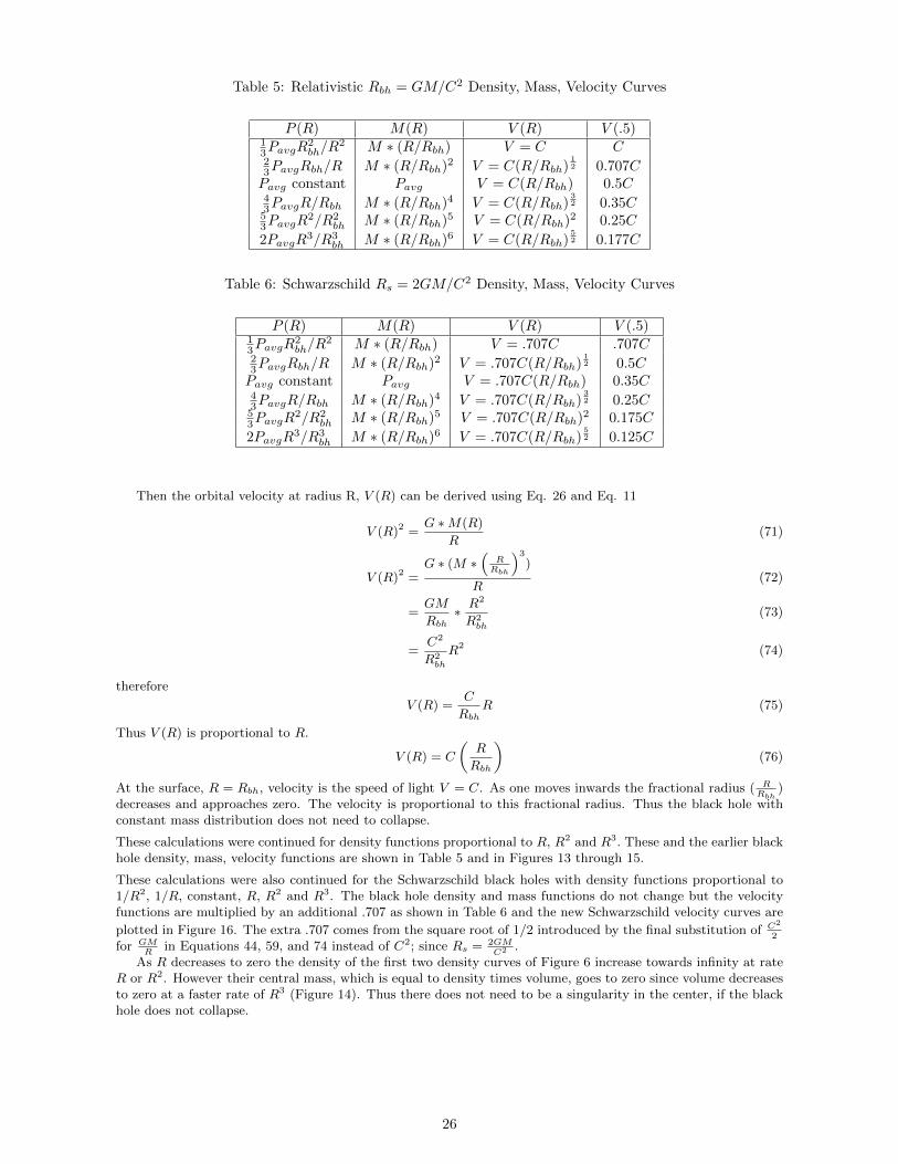
Table 5: Relativistic Rbh = GM/C2 Density, Mass, Velocity Curves

P (R) M(R) V (R) V (.5)13PavgR

2bh/R

2 M ∗ (R/Rbh) V = C C23PavgRbh/R M ∗ (R/Rbh)2 V = C(R/Rbh)

12 0.707C

Pavg constant Pavg V = C(R/Rbh) 0.5C43PavgR/Rbh M ∗ (R/Rbh)4 V = C(R/Rbh)

32 0.35C

53PavgR

2/R2bh M ∗ (R/Rbh)5 V = C(R/Rbh)2 0.25C

2PavgR3/R3

bh M ∗ (R/Rbh)6 V = C(R/Rbh)52 0.177C

Table 6: Schwarzschild Rs = 2GM/C2 Density, Mass, Velocity Curves

P (R) M(R) V (R) V (.5)13PavgR

2bh/R

2 M ∗ (R/Rbh) V = .707C .707C23PavgRbh/R M ∗ (R/Rbh)2 V = .707C(R/Rbh)

12 0.5C

Pavg constant Pavg V = .707C(R/Rbh) 0.35C43PavgR/Rbh M ∗ (R/Rbh)4 V = .707C(R/Rbh)

32 0.25C

53PavgR

2/R2bh M ∗ (R/Rbh)5 V = .707C(R/Rbh)2 0.175C

2PavgR3/R3

bh M ∗ (R/Rbh)6 V = .707C(R/Rbh)52 0.125C

Then the orbital velocity at radius R, V (R) can be derived using Eq. 26 and Eq. 11

V (R)2 =G ∗M(R)

R(71)

V (R)2 =G ∗ (M ∗

(RRbh

)3)

R(72)

=GM

Rbh∗ R

2

R2bh

(73)

=C2

R2bh

R2 (74)

therefore

V (R) =C

RbhR (75)

Thus V (R) is proportional to R.

V (R) = C

(R

Rbh

)(76)

At the surface, R = Rbh, velocity is the speed of light V = C. As one moves inwards the fractional radius ( RRbh

)decreases and approaches zero. The velocity is proportional to this fractional radius. Thus the black hole withconstant mass distribution does not need to collapse.

These calculations were continued for density functions proportional to R, R2 and R3. These and the earlier blackhole density, mass, velocity functions are shown in Table 5 and in Figures 13 through 15.

These calculations were also continued for the Schwarzschild black holes with density functions proportional to1/R2, 1/R, constant, R, R2 and R3. The black hole density and mass functions do not change but the velocityfunctions are multiplied by an additional .707 as shown in Table 6 and the new Schwarzschild velocity curves are

plotted in Figure 16. The extra .707 comes from the square root of 1/2 introduced by the final substitution of C2

2

for GMR

in Equations 44, 59, and 74 instead of C2; since Rs = 2GMC2 .

As R decreases to zero the density of the first two density curves of Figure 6 increase towards infinity at rateR or R2. However their central mass, which is equal to density times volume, goes to zero since volume decreasesto zero at a faster rate of R3 (Figure 14). Thus there does not need to be a singularity in the center, if the blackhole does not collapse.

26

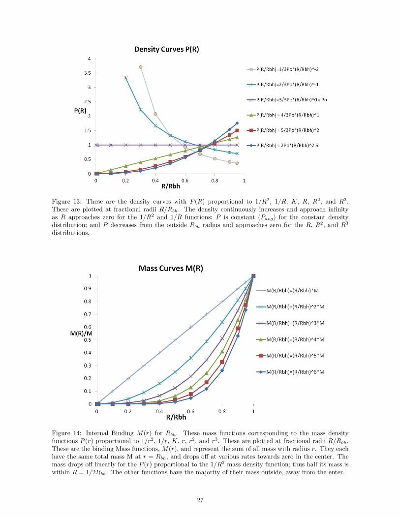
Figure 13: These are the density curves with P (R) proportional to 1/R2, 1/R, K, R, R2, and R3.These are plotted at fractional radii R/Rbh. The density continuously increases and approach infinityas R approaches zero for the 1/R2 and 1/R functions; P is constant (Pavg) for the constant densitydistribution; and P decreases from the outside Rbh radius and approaches zero for the R, R2, and R3

distributions.

Figure 14: Internal Binding M(r) for Rbh. These mass functions corresponding to the mass densityfunctions P (r) proportional to 1/r2, 1/r, K, r, r2, and r3. These are plotted at fractional radii R/Rbh.These are the binding Mass functions, M(r), and represent the sum of all mass with radius r. They eachhave the same total mass M at r = Rbh, and drops off at various rates towards zero in the center. Themass drops off linearly for the P (r) proportional to the 1/R2 mass density function; thus half its mass iswithin R = 1/2Rbh. The other functions have the majority of their mass outside, away from the enter.

27

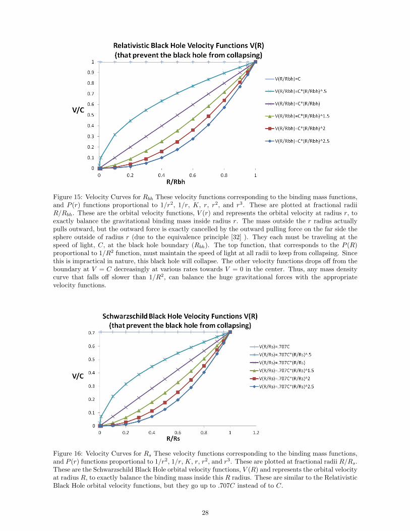
Figure 15: Velocity Curves for Rbh These velocity functions corresponding to the binding mass functions,and P (r) functions proportional to 1/r2, 1/r, K, r, r2, and r3. These are plotted at fractional radiiR/Rbh. These are the orbital velocity functions, V (r) and represents the orbital velocity at radius r, toexactly balance the gravitational binding mass inside radius r. The mass outside the r radius actuallypulls outward, but the outward force is exactly cancelled by the outward pulling force on the far side thesphere outside of radius r (due to the equivalence principle [32] ). They each must be traveling at thespeed of light, C, at the black hole boundary (Rbh). The top function, that corresponds to the P (R)proportional to 1/R2 function, must maintain the speed of light at all radii to keep from collapsing. Sincethis is impractical in nature, this black hole will collapse. The other velocity functions drops off from theboundary at V = C decreasingly at various rates towards V = 0 in the center. Thus, any mass densitycurve that falls off slower than 1/R2, can balance the huge gravitational forces with the appropriatevelocity functions.

Figure 16: Velocity Curves for Rs These velocity functions corresponding to the binding mass functions,and P (r) functions proportional to 1/r2, 1/r, K, r, r2, and r3. These are plotted at fractional radii R/Rs.These are the Schwarzschild Black Hole orbital velocity functions, V (R) and represents the orbital velocityat radius R, to exactly balance the binding mass inside this R radius. These are similar to the RelativisticBlack Hole orbital velocity functions, but they go up to .707C instead of to C.

28

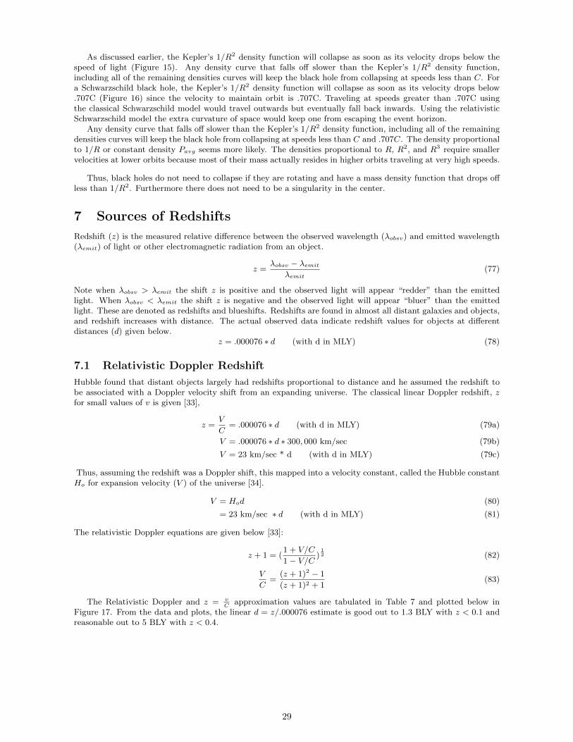
As discussed earlier, the Kepler’s 1/R2 density function will collapse as soon as its velocity drops below thespeed of light (Figure 15). Any density curve that falls off slower than the Kepler’s 1/R2 density function,including all of the remaining densities curves will keep the black hole from collapsing at speeds less than C. Fora Schwarzschild black hole, the Kepler’s 1/R2 density function will collapse as soon as its velocity drops below.707C (Figure 16) since the velocity to maintain orbit is .707C. Traveling at speeds greater than .707C usingthe classical Schwarzschild model would travel outwards but eventually fall back inwards. Using the relativisticSchwarzschild model the extra curvature of space would keep one from escaping the event horizon.

Any density curve that falls off slower than the Kepler’s 1/R2 density function, including all of the remainingdensities curves will keep the black hole from collapsing at speeds less than C and .707C. The density proportionalto 1/R or constant density Pavg seems more likely. The densities proportional to R, R2, and R3 require smallervelocities at lower orbits because most of their mass actually resides in higher orbits traveling at very high speeds.

Thus, black holes do not need to collapse if they are rotating and have a mass density function that drops offless than 1/R2. Furthermore there does not need to be a singularity in the center.

7 Sources of Redshifts

Redshift (z) is the measured relative difference between the observed wavelength (λobsv) and emitted wavelength(λemit) of light or other electromagnetic radiation from an object.

z =λobsv − λemit

λemit(77)

Note when λobsv > λemit the shift z is positive and the observed light will appear “redder” than the emittedlight. When λobsv < λemit the shift z is negative and the observed light will appear “bluer” than the emittedlight. These are denoted as redshifts and blueshifts. Redshifts are found in almost all distant galaxies and objects,and redshift increases with distance. The actual observed data indicate redshift values for objects at differentdistances (d) given below.

z = .000076 ∗ d (with d in MLY) (78)

7.1 Relativistic Doppler Redshift

Hubble found that distant objects largely had redshifts proportional to distance and he assumed the redshift tobe associated with a Doppler velocity shift from an expanding universe. The classical linear Doppler redshift, zfor small values of v is given [33],

z =V

C= .000076 ∗ d (with d in MLY) (79a)

V = .000076 ∗ d ∗ 300, 000 km/sec (79b)

V = 23 km/sec * d (with d in MLY) (79c)

Thus, assuming the redshift was a Doppler shift, this mapped into a velocity constant, called the Hubble constantHo for expansion velocity (V ) of the universe [34].

V = Hod (80)

= 23 km/sec ∗ d (with d in MLY) (81)

The relativistic Doppler equations are given below [33]:

z + 1 = (1 + V/C

1− V/C )12 (82)

V

C=

(z + 1)2 − 1

(z + 1)2 + 1(83)

The Relativistic Doppler and z = vC

approximation values are tabulated in Table 7 and plotted below inFigure 17. From the data and plots, the linear d = z/.000076 estimate is good out to 1.3 BLY with z < 0.1 andreasonable out to 5 BLY with z < 0.4.

29

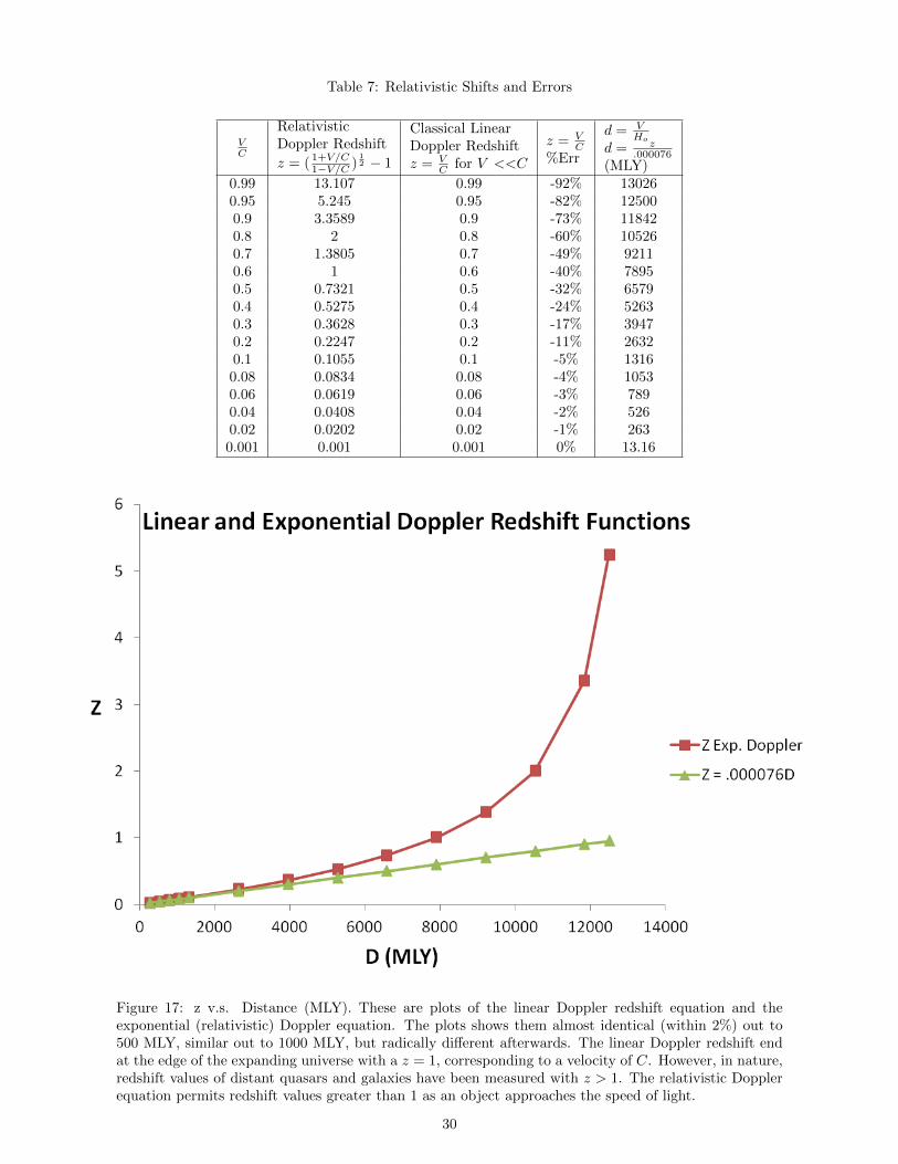
Table 7: Relativistic Shifts and Errors

VC

RelativisticDoppler Redshift

z = ( 1+V/C1−V/C )

12 − 1

Classical LinearDoppler Redshiftz = V

C for V <<C

z = VC

%Err

d = VHo

d = z.000076

(MLY)0.99 13.107 0.99 -92% 130260.95 5.245 0.95 -82% 125000.9 3.3589 0.9 -73% 118420.8 2 0.8 -60% 105260.7 1.3805 0.7 -49% 92110.6 1 0.6 -40% 78950.5 0.7321 0.5 -32% 65790.4 0.5275 0.4 -24% 52630.3 0.3628 0.3 -17% 39470.2 0.2247 0.2 -11% 26320.1 0.1055 0.1 -5% 13160.08 0.0834 0.08 -4% 10530.06 0.0619 0.06 -3% 7890.04 0.0408 0.04 -2% 5260.02 0.0202 0.02 -1% 2630.001 0.001 0.001 0% 13.16

Figure 17: z v.s. Distance (MLY). These are plots of the linear Doppler redshift equation and theexponential (relativistic) Doppler equation. The plots shows them almost identical (within 2%) out to500 MLY, similar out to 1000 MLY, but radically different afterwards. The linear Doppler redshift endat the edge of the expanding universe with a z = 1, corresponding to a velocity of C. However, in nature,redshift values of distant quasars and galaxies have been measured with z > 1. The relativistic Dopplerequation permits redshift values greater than 1 as an object approaches the speed of light.

30

The equations depart after 1.3 BLY with z values growing exponentially, where the linear approximationis limited to z = 1 at the perceived radius of the universe. Astronomers use these exponentially increasing zvalues to explain the most distant quasars (with z = 7) without requiring them to be at 92 BLY using the linearapproximation equation (e.g. z = 7 = .000076dMLY ; d = 7/.000076 = 92000MLY )

Before the year 2000, astronomers only had accurate distance measures based on redshifts to supernovae outto about 0.5 BLY. However, in 2003, accurate super nova measurements have been extended out to about 1.3BLY and the light appears to be following the theoretical non-linear relativistic curve [35]. That is, it matchesthe relativistic Doppler equation. But as indicated by Table 7, at this point, the linear equation is only off by lessthan 5%.

However these researchers then plugged these same data into their best expanding universe models and couldn’tfind a fit unless they tweaked terms or included an accelerated expansion. They chose to introduce a new energysource called Dark Energy to preserve their expanding universe model. Normally, when one’s best model doesnot fit the data, they should consider abandoning their model. Hopefully, after reviewing Theorem 1 of Section 4which disproves the expanding universe, cosmologist might want to reconsider their model.

Even if the expanding universe and Doppler shift velocity interpretation are invalid, the observed redshiftvalues of z = .000076 ∗ d (with d in MLY) still need to be explained.

Without a relativistic Doppler shift equation cosmologist might have concluded that the shift was linear outto their best data measurements, but perhaps with some slight deviations of z starting to show up at .5 to 1.3BLYs. They would then look for a physical cause for these slightly increased z values in the past. Or they mightfind a different “best” fit that better matches the more distant data, and have the closer (more recent) pointsshowing a slightly lower redshift value than expected (perhaps due to a contracting universe). This paper willpursue both: investigating the linear redshift z = .000076 ∗ d MLY function and also curves that depart startingaround .5 BLY. This paper will also pursue different explanation for the large redshifts of quasars.

7.2 Cosmological Redshift

Some scientists replaced the Doppler based redshift explanation with a cosmological redshift explanation wherethe velocities increases because space itself is expanding. This allows for velocity values higher than C, withoutviolating the speed of light.

Since the Cosmological redshift is based on an expanding universe, the cosmological shift would actuallybecome zero in a non-expanding universe and a blueshift in a rapidly collapsing universe. In any event, both theDoppler based redshift and Cosmological based redshifts would go away in a non-expanding universe.

7.3 Relativistic Transverse Redshift

In addition to relativistic Doppler shift due to the speed of light moving away from the observer, a relativistictransverse redshift would also be observed due to time dilation (time slowing down) if the universe was rapidlyrotating at relativistic speeds to keep from collapsing. Einstein’s relativistic transverse redshift (zt) equations are[36]:

zt =1

(1− V 2/C2)12

− 1 (84)

V

C=

(1− 1

(zt + 1)2

) 12

(85)

These are shown compared to the relativistic Doppler shifts Figures 18a and 18b and Table 8. Note that theTransverse shift is considerably smaller than the Doppler shift. Thus, to get the observed redshift z seen inDoppler, the transverse velocity would need to be greater (.e.g. zt = .25 at V = .6C for transverse instead ofV = .22C for Doppler).

The rotating velocity curves (from Figure 15) are repeated in Figure 19 along with their matching translationalredshifts curves in Figure 20. All the velocity curves create relativistic transverse redshifts as their speeds approachthe speed of light C. The redshift for the V = C curve was not plotted since this would always have infinite redshift.Values are plotted up to .95C. Higher values of zt could be achieved by approaching closer to the speed of light(e.g. .99C). Thus, any of these speed curves can cause high zt values, near the edge of the Black hole.

31

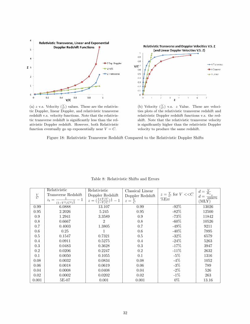
(a) z v.s. Velocity (VC

) values. These are the relativis-tic Doppler, linear Doppler, and relativistic transverseredshift v.s. velocity functions. Note that the relativis-tic transverse redshift is significantly less than the rel-ativistic Doppler redshift. However, both Relativisticfunction eventually go up exponentially near V = C.

(b) Velocity (VC

) v.s. z Value. These are veloci-ties plots of the relativistic transverse redshift andrelativistic Doppler redshift functions v.s. the red-shift. Note that the relativistic transverse velocityis significantly higher than the relativistic Dopplervelocity to produce the same redshift.

Figure 18: Relativistic Transverse Redshift Compared to the Relativistic Doppler Shifts

Table 8: Relativistic Shifts and Errors

VC

RelativisticTransverse Redshiftzt = 1

(1−V 2/C2)12− 1

RelativisticDoppler Redshift

z = ( 1+V/C1−V/C )

12 − 1

Classical LinearDoppler Redshiftz = V

C

z = VC for V <<C

%Err

d = VHo

d = z.000076

(MLY)

0.99 6.0888 13.107 0.99 -92% 130260.95 2.2026 5.245 0.95 -82% 125000.9 1.2941 3.3589 0.9 -73% 118420.8 0.6667 2 0.8 -60% 105260.7 0.4003 1.3805 0.7 -49% 92110.6 0.25 1 0.6 -40% 78950.5 0.1547 0.7321 0.5 -32% 65790.4 0.0911 0.5275 0.4 -24% 52630.3 0.0483 0.3628 0.3 -17% 39470.2 0.0206 0.2247 0.2 -11% 26320.1 0.0050 0.1055 0.1 -5% 13160.08 0.0032 0.0834 0.08 -4% 10520.06 0.0018 0.0619 0.06 -3% 7890.04 0.0008 0.0408 0.04 -2% 5260.02 0.0002 0.0202 0.02 -1% 2630.001 5E-07 0.001 0.001 0% 13.16

32

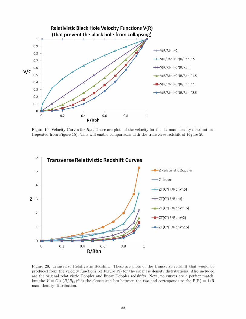
Figure 19: Velocity Curves for Rbh. These are plots of the velocity for the six mass density distributions(repeated from Figure 15). This will enable comparisons with the transverse redshift of Figure 20.

Figure 20: Transverse Relativistic Redshift. These are plots of the transverse redshift that would beproduced from the velocity functions (of Figure 19) for the six mass density distributions. Also includedare the original relativistic Doppler and linear Doppler redshifts. Note, no curves are a perfect match,but the V = C ∗ (R/Rbh).5 is the closest and lies between the two and corresponds to the P(R) = 1/Rmass density distribution.

33

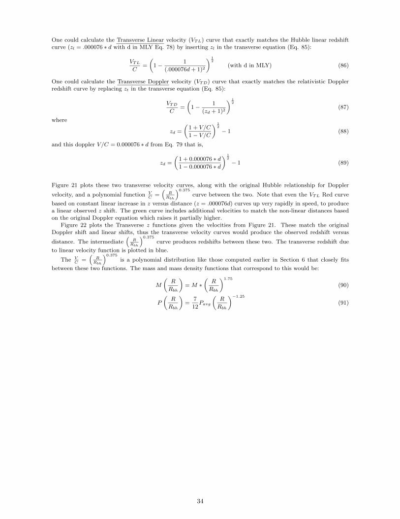
One could calculate the Transverse Linear velocity (VTL) curve that exactly matches the Hubble linear redshiftcurve (zl = .000076 ∗ d with d in MLY Eq. 78) by inserting zl in the transverse equation (Eq. 85):

VTLC

=

(1− 1

(.000076d+ 1)2

) 12

(with d in MLY) (86)

One could calculate the Transverse Doppler velocity (VTD) curve that exactly matches the relativistic Dopplerredshift curve by replacing zt in the transverse equation (Eq. 85):

VTDC

=

(1− 1

(zd + 1)2

) 12

(87)

where

zd =

(1 + V/C

1− V/C

) 12

− 1 (88)

and this doppler V/C = 0.000076 ∗ d from Eq. 79 that is,

zd =

(1 + 0.000076 ∗ d1− 0.000076 ∗ d

) 12

− 1 (89)

Figure 21 plots these two transverse velocity curves, along with the original Hubble relationship for Doppler

velocity, and a polynomial function VC

=(

RRbh

)0.375curve between the two. Note that even the VTL Red curve

based on constant linear increase in z versus distance (z = .000076d) curves up very rapidly in speed, to producea linear observed z shift. The green curve includes additional velocities to match the non-linear distances basedon the original Doppler equation which raises it partially higher.

Figure 22 plots the Transverse z functions given the velocities from Figure 21. These match the originalDoppler shift and linear shifts, thus the transverse velocity curves would produce the observed redshift versus

distance. The intermediate(

RRbh

)0.375curve produces redshifts between these two. The transverse redshift due

to linear velocity function is plotted in blue.

The VC

=(

RRbh

)0.375is a polynomial distribution like those computed earlier in Section 6 that closely fits

between these two functions. The mass and mass density functions that correspond to this would be:

M

(R

Rbh

)= M ∗

(R

Rbh

)1.75

(90)

P

(R

Rbh

)=

7

12Pavg

(R

Rbh

)−1.25

(91)

34

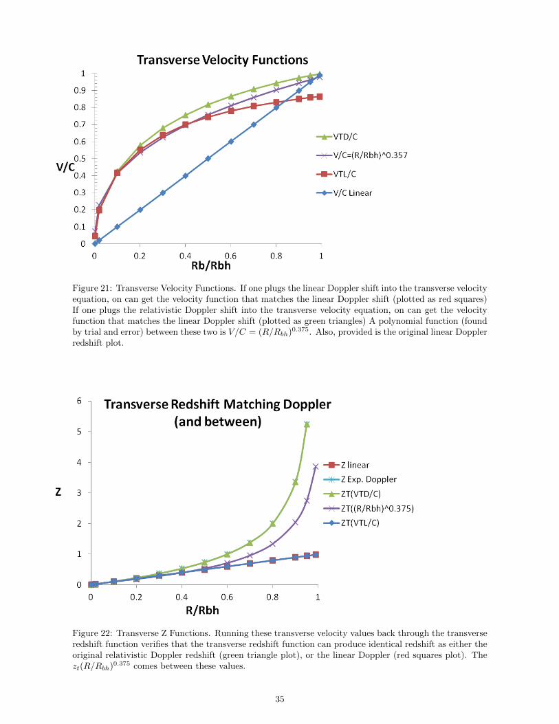
Figure 21: Transverse Velocity Functions. If one plugs the linear Doppler shift into the transverse velocityequation, on can get the velocity function that matches the linear Doppler shift (plotted as red squares)If one plugs the relativistic Doppler shift into the transverse velocity equation, on can get the velocityfunction that matches the linear Doppler shift (plotted as green triangles) A polynomial function (foundby trial and error) between these two is V/C = (R/Rbh)0.375. Also, provided is the original linear Dopplerredshift plot.

Figure 22: Transverse Z Functions. Running these transverse velocity values back through the transverseredshift function verifies that the transverse redshift function can produce identical redshift as either theoriginal relativistic Doppler redshift (green triangle plot), or the linear Doppler (red squares plot). Thezt(R/Rbh)0.375 comes between these values.

35

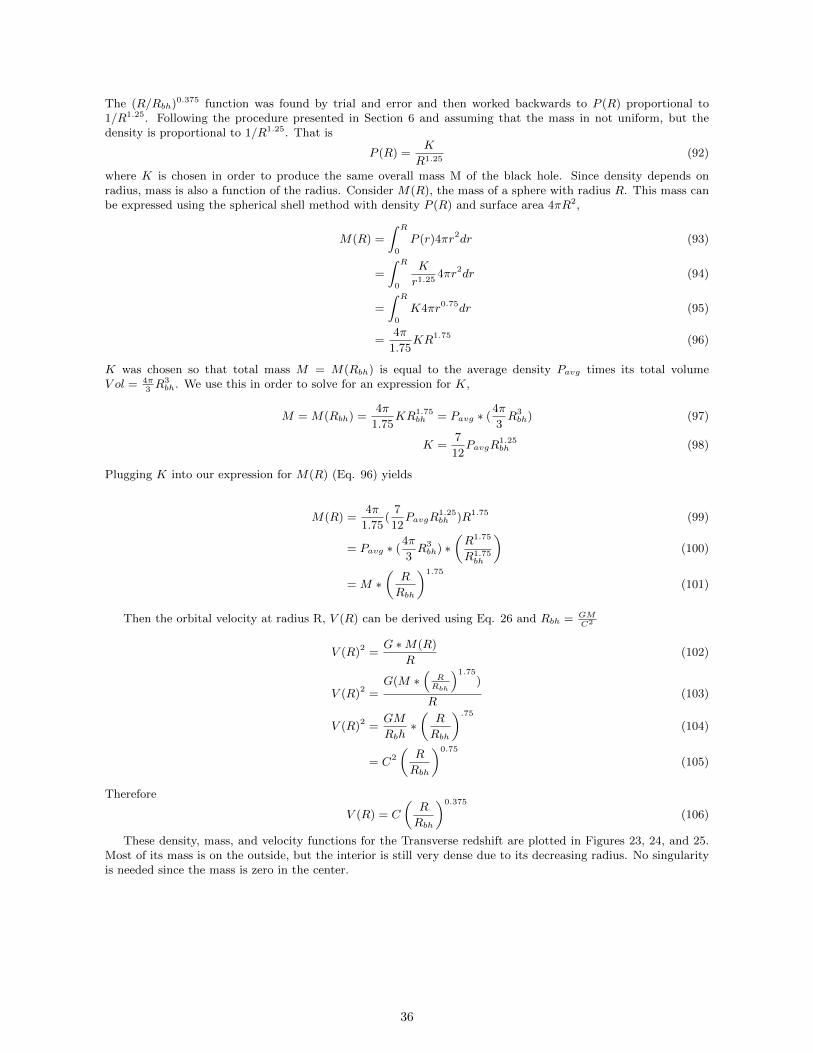
The (R/Rbh)0.375 function was found by trial and error and then worked backwards to P (R) proportional to1/R1.25. Following the procedure presented in Section 6 and assuming that the mass in not uniform, but thedensity is proportional to 1/R1.25. That is

P (R) =K

R1.25(92)

where K is chosen in order to produce the same overall mass M of the black hole. Since density depends onradius, mass is also a function of the radius. Consider M(R), the mass of a sphere with radius R. This mass canbe expressed using the spherical shell method with density P (R) and surface area 4πR2,

M(R) =

∫ R

0

P (r)4πr2dr (93)

=

∫ R

0

K

r1.254πr2dr (94)

=

∫ R

0

K4πr0.75dr (95)

=4π

1.75KR1.75 (96)

K was chosen so that total mass M = M(Rbh) is equal to the average density Pavg times its total volumeV ol = 4π

3R3bh. We use this in order to solve for an expression for K,

M = M(Rbh) =4π

1.75KR1.75

bh = Pavg ∗ (4π

3R3bh) (97)

K =7

12PavgR

1.25bh (98)

Plugging K into our expression for M(R) (Eq. 96) yields

M(R) =4π

1.75(

7

12PavgR

1.25bh )R1.75 (99)

= Pavg ∗ (4π

3R3bh) ∗

(R1.75

R1.75bh

)(100)

= M ∗(R

Rbh

)1.75

(101)

Then the orbital velocity at radius R, V (R) can be derived using Eq. 26 and Rbh = GMC2

V (R)2 =G ∗M(R)

R(102)

V (R)2 =G(M ∗

(RRbh

)1.75)

R(103)

V (R)2 =GM

Rbh∗(R

Rbh

).75(104)

= C2

(R

Rbh

)0.75

(105)

Therefore

V (R) = C

(R

Rbh

)0.375

(106)

These density, mass, and velocity functions for the Transverse redshift are plotted in Figures 23, 24, and 25.Most of its mass is on the outside, but the interior is still very dense due to its decreasing radius. No singularityis needed since the mass is zero in the center.

36

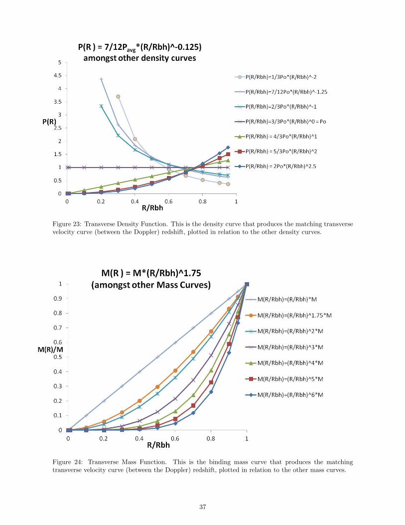
Figure 23: Transverse Density Function. This is the density curve that produces the matching transversevelocity curve (between the Doppler) redshift, plotted in relation to the other density curves.

Figure 24: Transverse Mass Function. This is the binding mass curve that produces the matchingtransverse velocity curve (between the Doppler) redshift, plotted in relation to the other mass curves.

37

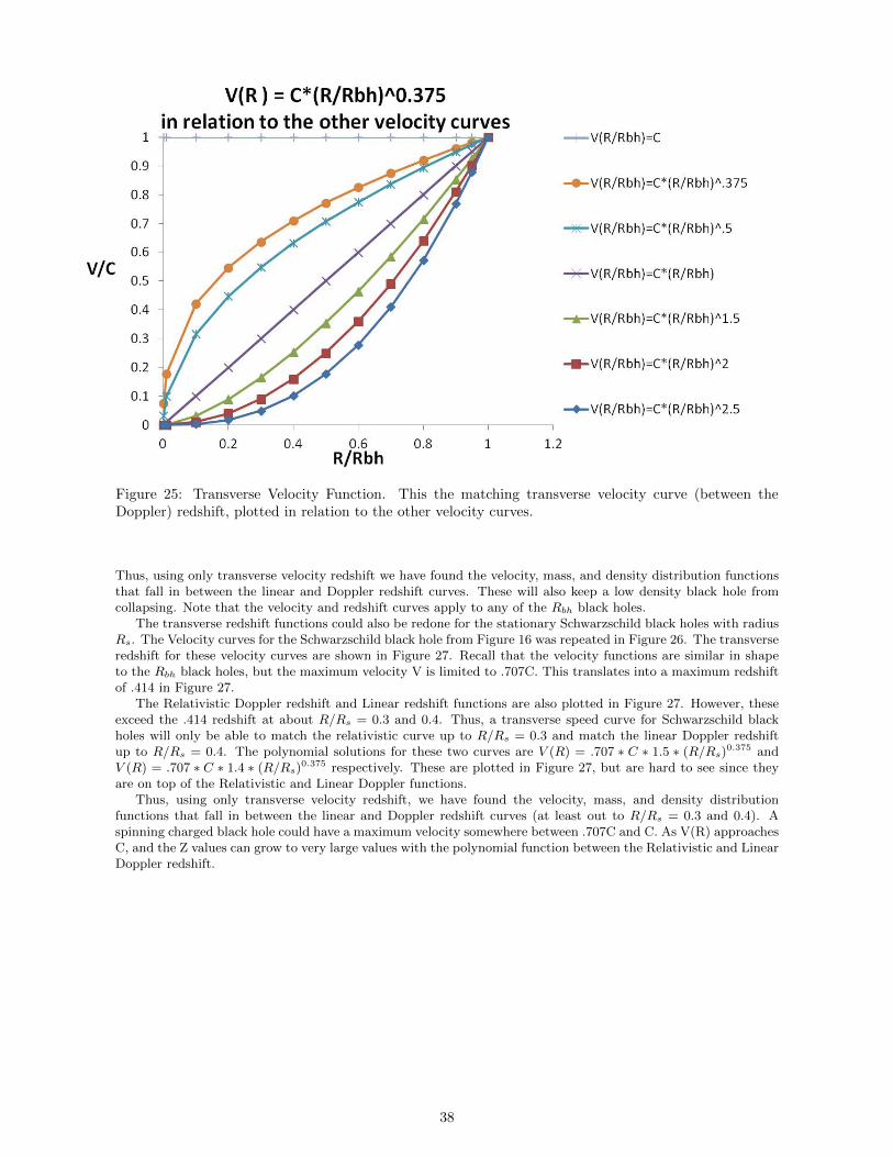
Figure 25: Transverse Velocity Function. This the matching transverse velocity curve (between theDoppler) redshift, plotted in relation to the other velocity curves.

Thus, using only transverse velocity redshift we have found the velocity, mass, and density distribution functionsthat fall in between the linear and Doppler redshift curves. These will also keep a low density black hole fromcollapsing. Note that the velocity and redshift curves apply to any of the Rbh black holes.

The transverse redshift functions could also be redone for the stationary Schwarzschild black holes with radiusRs. The Velocity curves for the Schwarzschild black hole from Figure 16 was repeated in Figure 26. The transverseredshift for these velocity curves are shown in Figure 27. Recall that the velocity functions are similar in shapeto the Rbh black holes, but the maximum velocity V is limited to .707C. This translates into a maximum redshiftof .414 in Figure 27.

The Relativistic Doppler redshift and Linear redshift functions are also plotted in Figure 27. However, theseexceed the .414 redshift at about R/Rs = 0.3 and 0.4. Thus, a transverse speed curve for Schwarzschild blackholes will only be able to match the relativistic curve up to R/Rs = 0.3 and match the linear Doppler redshiftup to R/Rs = 0.4. The polynomial solutions for these two curves are V (R) = .707 ∗ C ∗ 1.5 ∗ (R/Rs)

0.375 andV (R) = .707 ∗ C ∗ 1.4 ∗ (R/Rs)

0.375 respectively. These are plotted in Figure 27, but are hard to see since theyare on top of the Relativistic and Linear Doppler functions.

Thus, using only transverse velocity redshift, we have found the velocity, mass, and density distributionfunctions that fall in between the linear and Doppler redshift curves (at least out to R/Rs = 0.3 and 0.4). Aspinning charged black hole could have a maximum velocity somewhere between .707C and C. As V(R) approachesC, and the Z values can grow to very large values with the polynomial function between the Relativistic and LinearDoppler redshift.

38

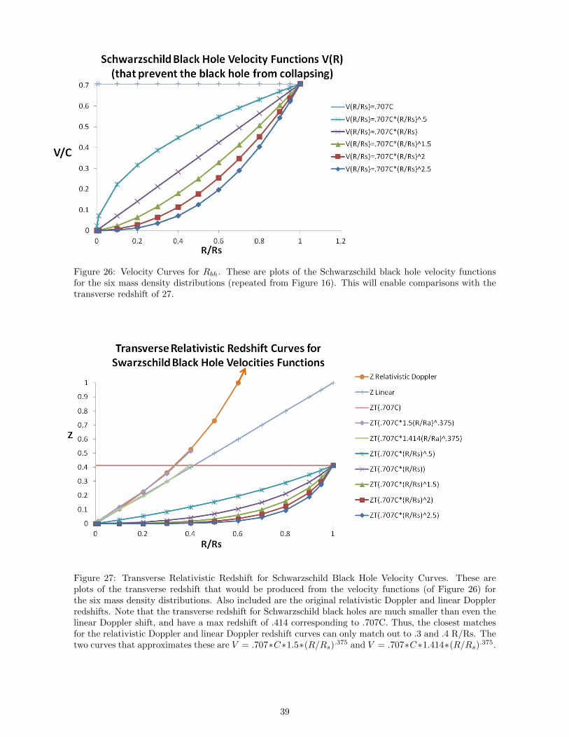
Figure 26: Velocity Curves for Rbh. These are plots of the Schwarzschild black hole velocity functionsfor the six mass density distributions (repeated from Figure 16). This will enable comparisons with thetransverse redshift of 27.

Figure 27: Transverse Relativistic Redshift for Schwarzschild Black Hole Velocity Curves. These areplots of the transverse redshift that would be produced from the velocity functions (of Figure 26) forthe six mass density distributions. Also included are the original relativistic Doppler and linear Dopplerredshifts. Note that the transverse redshift for Schwarzschild black holes are much smaller than even thelinear Doppler shift, and have a max redshift of .414 corresponding to .707C. Thus, the closest matchesfor the relativistic Doppler and linear Doppler redshift curves can only match out to .3 and .4 R/Rs. Thetwo curves that approximates these are V = .707∗C∗1.5∗(R/Rs).375 and V = .707∗C∗1.414∗(R/Rs).375.

39

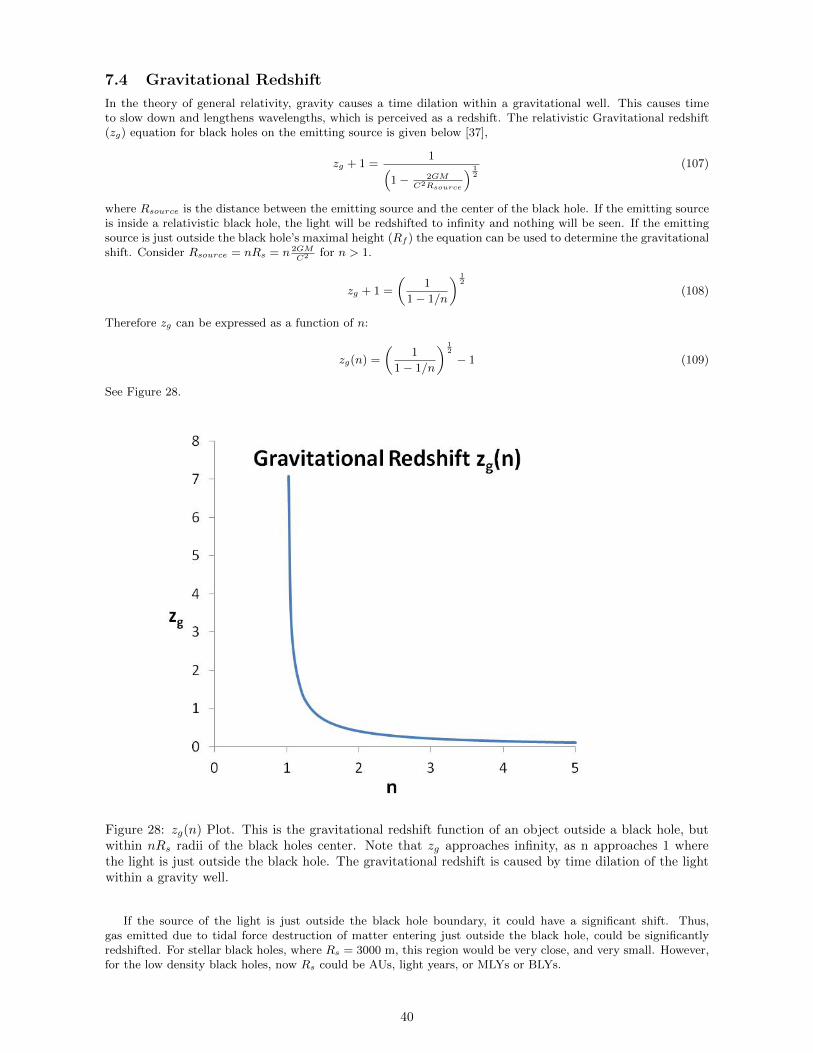
7.4 Gravitational Redshift

In the theory of general relativity, gravity causes a time dilation within a gravitational well. This causes timeto slow down and lengthens wavelengths, which is perceived as a redshift. The relativistic Gravitational redshift(zg) equation for black holes on the emitting source is given below [37],

zg + 1 =1(

1− 2GMC2Rsource

) 12

(107)

where Rsource is the distance between the emitting source and the center of the black hole. If the emitting sourceis inside a relativistic black hole, the light will be redshifted to infinity and nothing will be seen. If the emittingsource is just outside the black hole’s maximal height (Rf ) the equation can be used to determine the gravitationalshift. Consider Rsource = nRs = n 2GM

C2 for n > 1.

zg + 1 =

(1

1− 1/n

) 12

(108)

Therefore zg can be expressed as a function of n:

zg(n) =

(1

1− 1/n

) 12

− 1 (109)

See Figure 28.

Figure 28: zg(n) Plot. This is the gravitational redshift function of an object outside a black hole, butwithin nRs radii of the black holes center. Note that zg approaches infinity, as n approaches 1 wherethe light is just outside the black hole. The gravitational redshift is caused by time dilation of the lightwithin a gravity well.

If the source of the light is just outside the black hole boundary, it could have a significant shift. Thus,gas emitted due to tidal force destruction of matter entering just outside the black hole, could be significantlyredshifted. For stellar black holes, where Rs = 3000 m, this region would be very close, and very small. However,for the low density black holes, now Rs could be AUs, light years, or MLYs or BLYs.

40

Also, being inside a small rotating low density black hole does not preclude adjacent low density black holesfrom contributing additional redshift. An additional larger encapsulating container low density black hole at largerradii surrounding the original black hole and its neighbors could provide even more redshift. Additional adjacentcontainer black holes and larger nested container low density back holes can provide additional gravitationalredshifts, and also contribute to the observable linear redshift that increases with distance. That is, the universecould be considered a nested set of low density black holes.

7.5 Intrinsic Redshift of Interstellar Space

Independent of this paper, there has been a growing debate about replacing the Doppler shift interpretation ofredshift with an intrinsic redshift of space itself (or its interstellar medium) that causes light to redshift linearlywith distance, roughly matching the linear Hubble redshift approximation equation. Marmet et al. [38] containsa survey of 59 of these theorized intrinsic redshift mechanism, including:

1. Gravitational Drag

2. Interaction of a massive Photon with Vacuum Particles

3. Interaction Between the Photon Energy and Vacuum Space

4. Light interaction with Microwaves and Radio Waves

5. Photon Decay

6. Finite Conductivity of Space

7. Photon-Graviton Interaction

8. Electrogravitational Coupling

9. Gravitomagnetic Effect

10. Interaction with the Intergalactic Gas

These redshift concepts are attempting to find a real causal mechanism within the laws of physics to describethe linearly increasing redshift with distance.

To date, the Doppler shift and the expanding universe has been the leading redshift mechanism by mostcosmologists. However, after disproving the expanding universe model in this paper, along with its Doppler shiftinterpretation, one of the intrinsic redshift mechanism may get a closer reading.

If the linear redshift is just a function of space itself, then the redshift largely matches the observed phenomena.However, at present, we currently don’t know the true source of the intrinsic redshift, assuming that intrisicredshift is real. For the remainder of this paper, this paper will consider the following five possible candidatesfor intrinsic redshift: Bremsstrahlung radiation, Induced Electric Dipole redshift (IEDRS), simple charge basedintrinsic redshift, gravitational drag, and bending redshifts.

7.5.1 Bremsstrahlung Intrinsic Redshift

In the literature, there is a new Non Doppler effect redshift based on Bremsstrahlung radiation. Low densityparticles in space scatter light, in addition to the Compton scattering effect, the light can accelerate electrons.According to electromagnetic theory, any accelerated charge must emit Bremsstrahlung radiation. Although theenergy emitted due to such acceleration is extremely small, the energy lost by Bremsstrahlung causes a slightredshift.

Bremsstrahlung radiation is reported to impact all wavelengths equally and thus will appear similar to Dopplerredshift. An average density of the order of 0.01 atoms per cubic centimeter is sufficient to produce, on the Planckspectrum, an effect equivalent to that of a Doppler shift in agreement with the Hubble constant[39].

If the Bremsstrahlung redshift is valid, no other mechanism is needed to match the perceived linear Dopplershift as long as the interstellar density is approximately .01 atoms per cubic centimeter.

7.5.2 Induced Electric Dipole Redshift

Also in the literature, there is another Non Doppler effect redshift based on electric charge effects on light [40]. Toquote that paper, “Small induced dipole forces acting on photons can account for the red-shift. In atomic physics,gamma rays are known to split (electron positron pair production) while in the intense central electric fields ofatomic nuclei and charged subatomic particles. The photon energy is converted to mass and kinetic energy, butdue to the law of conservation of charge, the (-,+) charge pair must have been contained within the photon priorto pair production. It must be the induced electric dipole force that forces the charge pair to separate. Lessenergetic photons do not have sufficient energy for pair production (1.02 MeV is the minimum energy required),but they must similarly contain a (-,+) charge pair. This pair will separate slightly while in any non-uniformelectric field; causing an attractive force (the induced electric dipole force is always attractive). This small forceacting on photons as they travel over astronomical distances will reduce photon energy (the red-shift)”.

If Induced Electric Dipole redshift (IEDRS) theory is valid, no other redshift is needed to match the linearDoppler redshift.

41

7.5.3 Charge Based redshift

A charged particle in a changing electro-magnetic field will be accelerated. This energy needs to come from thelight, and will change the electromagnetic energy by redshifting the light. Thus, when light passes through chargedparticles, the light will be redshifted. Thus, light passing through ions in space should slow down and produce aslight redshift.

Even a neutral hydrogen atom consists of a charged electron and a charged proton, when considered separately.The electromagnetic field (e.g. light) would accelerate each of these slightly, but would consume light energy andproduce a slight redshift.

7.5.4 Gravitational Drag (Shapiro Effect)

Dr. Irwin I. Shapiro of the Lincoln Labs of the Massachusetts Institute of Technology, stated “...according tothe general theory, the speed of a light wave depends on the strength of the gravitational potential along itspath.” Light will experience a small, cumulative deceleration from the forces of this gravitational field acting atlong range. This does not smear the light nor provide a visible signature, but only a gravitationally inducedtime delay. The photon’s interaction with gravity does not alter its path, nor change its characteristic, except bygradually decreasing its velocity and energy, showing up as a redshift [38, 41].

7.5.5 Light Bending

Since light also has momentum, the simple process of bending of light, independent of what actually caused thebending, may cause the momentum to change, and thus may cause its energy to change and be redshifted.

7.6 Other Sources of redshift

Light reddening: occurs when light hits particles in space. They cause the light to redden, but not shift. As-tronomers are able to account for this phenomenon and these are not included in the redshift values.

Index of Refraction: n = CV

: Light traveling through a medium (e.g. for air, n= 1.000277) will slow downand thus be redshifted. This would put n = C

V; Interstellar gas is a medium, but could cause a slow down.

However, the index of refraction slow down is constant, not accumulative, unless the gas gets increasing densefarther away. Thus these are not believed to cause the linear redshift.

7.7 Quasars Redshift

The most distant objects visible (as measured by redshift z values) are Quasi-stellar radio sources (“quasars”),which are very energetic distant active galactic cores. A quasar is believed to be a compact region in the centerof a massive galaxy, that surrounds its central region with a dust cloud the size that is 10–10,000 times theSchwarzschild radius of the black hole. Since some quasars display changes in luminosity very rapidly from side toside, quasars are estimated to be not much larger than the Solar System (50 au = 7 light hours) [42]. Quasars areextremely luminous objects with redshifts between 0.056 and 7.085 [43, 44]. There is much debate as to whetherquasars are large, luminous, distant objects or smaller, less luminous, closer objects.

In either event, their redshifts will need to be created by transverse redshifts or from gravitational redshiftsfrom localized black holes, or intrinsic redshifts, or a combination of these redshifts.

7.7.1 Intrinsic Redshift

Using only the linear distance redshift equation (Eq. 78) applicable to all the intrinsic redshift mechanisms, weget an equation for distance as a function of z:

d(z) =z

.000076(with d in MLY) (110)

d(.056) =0.056

.000076= 737 MLY (111)

d(7.085) =7.085

.000076= 92 BLY (112)

The linear equation generates extremely large values of d well beyond the current big bang estimates of 13.8 BLYfor the size of the universe. However, now that the big bang is disproven, the universe could go out to 92 BLYsince the big bang date of 13.8 is not necessarily valid. The universe would also almost match the visible densityof Table 2. However, a quasar would have to be extremely bright to be seen at a 92 BLY distance.

42

7.7.2 Transverse Redshift for Quasars

Using the transverse redshift equation (Eq. 85) we get an equation for V/C as a function of z:

V

C(z) =

(1− 1

(z + 1)2

) 12

(113a)

V

C(0.056) =

(1− 1

(0.056 + 1)2

) 12

= .321 (113b)

Therefore a quasar must be traveling horizontally around us at a velocity of V = .321C to produce the redshiftof z = 0.056. If was assume we are somewhere near the center of a black hole with radius 13.8 BLY we can solvefor its distance using Eq. 106:

V

C=

(R

Rbh

).375= .321 (113c)(

R

Rbh

)= .3218/3 = .0487 (113d)

d = 13.8

(R

Rbh

)= 672 MLY (113e)

Similarly for the largest z value:

V

C(7.085) =

(1− 1

(7.085 + 1)2

) 12

= .992 (114a)

V

C=

(R

Rbh

).375= .992 (114b)(

R

Rbh

)= .9928/3 = .978 (114c)

d = 13.8

(R

Rbh

)= 13.5 BLY (114d)

This quasar would be traveling with velocity of V = 0.992C and at a distance of 13.5 BLY. Thus, just thetransverse redshift could explain the high redshifts and bring them in closer.

7.7.3 Gravitational Redshift for Quasars

Using the gravitation redshift equation (Eq. 109), one can derive an equation for n as function of z:

zg(n) =

(1

1− 1/n

) 12

− 1 (115)

n(z) =

(1− 1

(z + 1)2

)−1

(116)

n(0.056) =

(1− 1

(z 0.056 + 1)2

)−1

= 9.7 (117)

Then R = nRs = 9.7Rs. Assuming the the quasar radius is R = 7 Light Hours then Rs = 7/9.7 = 0.72 Light

Hours and M = RsC2

2G= 0.5 B SM. This is just enough to cover the “closest” quasars with the lowest redshifts.

Similarly for the largest values, z = 7.085,

n(7.085) =

(1− 1

(z 7.085 + 1)2

)−1

= 1.016 (118)

Assuming the the quasar radius is R = 7 Light Hours then Rs = 7/1.016 = 6.89 Light Hours and M = RsC2

2G= 5

B SM. Thus, the entire quasar redshift can come from gravitational redshift.Quasars are only perceived as far away due to their high redshift. They would have to be very large to be seen

at that great a distance. However, if the source of the redshift is gravitational redshift, then quasars can be muchcloser and smaller. That said, since there are examples of gravitational lens duplication of quasars by interveninggalaxies, Quasars are at least outside our galaxy, and beyond the next, and possibly beyond many more.

The apparent magnitude of quasars are about 19±4 ([43]) shown in Figure 29a. Since we don’t know if they areclose or far away, we can’t plot their z shift versus distance. Plots of number and apparent magnitudes are shown

43

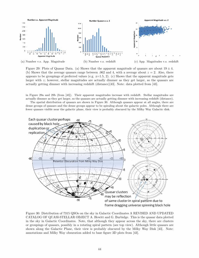
(a) Number v.s. App. Magnitude (b) Number v.s. redshift (c) App. Magnitudes v.s. redshift

Figure 29: Plots of Quasar Data. (a) Shows that the apparent magnitude of quasars are about 19 ± 4.(b) Shows that the average quasars range between .062 and 4, with a average about z = 2. Also, thereappears to be groupings of preferred values (e.g. z=1.5, 2). (c) Shows that the apparent magnitude getslarger with z; however, stellar magnitudes are actually dimmer as they get larger, so the quasars areactually getting dimmer with increasing redshift (distance)[43]. Note: data plotted from [43].

in Figure 29a and 29b (from [43]). Their apparent magnitudes increase with redshift. Stellar magnitudes areactually dimmer as they get larger, so the quasars are actually getting dimmer with increasing redshift (distance).

The spatial distribution of quasars are shown in Figure 30. Although quasars appear at all angles, there aredense groups of quasars and the dense groups appear to be spiraling about the galactic poles. Although there arefewer quasars visible near the galactic plane, their view is probably obscured by the Milky Way Galactic disk.

Figure 30: Distribution of 7315 QSOs on the sky in Galactic Coordinates A REVISED AND UPDATEDCATALOG OF QUASI-STELLAR OBJECT A. Hewitt and G. Burbidge. This is the quasar data plottedin the sky in Galactic Coordinates. Note, that although they appear across the sky, there are clustersor groupings of quasars, possibly in a rotating spiral pattern (see top view). Although little quasars areshown along the Galactic Plane, their view is probably obscured by the Milky Way Disk [43]. Note:annotations and Milky Way obsuration added to base figure 3D plots from [43].

44

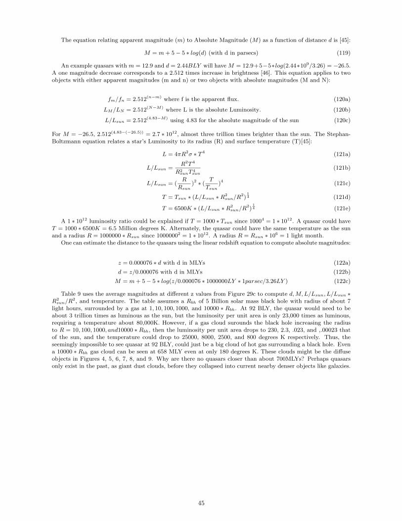
The equation relating apparent magnitude (m) to Absolute Magnitude (M) as a function of distance d is [45]:

M = m+ 5− 5 ∗ log(d) (with d in parsecs) (119)

An example quasars with m = 12.9 and d = 2.44BLY will have M = 12.9+5−5∗ log(2.44∗109/3.26) = −26.5.A one magnitude decrease corresponds to a 2.512 times increase in brightness [46]. This equation applies to twoobjects with either apparent magnitudes (m and n) or two objects with absolute magnitudes (M and N):

fm/fn = 2.512(n−m) where f is the apparent flux. (120a)

LM/LN = 2.512(N−M) where L is the absolute Luminosity. (120b)

L/Lsun = 2.512(4.83−M) using 4.83 for the absolute magnitude of the sun (120c)

For M = −26.5, 2.512(4.83−(−26.5)) = 2.7 ∗ 1012, almost three trillion times brighter than the sun. The Stephan-Boltzmann equation relates a star’s Luminosity to its radius (R) and surface temperature (T)[45]:

L = 4πR2σ ∗ T 4 (121a)

L/Lsun =R2T 4

R2sunT 4

sun

(121b)

L/Lsun = (R

Rsun)2 ∗ (

T

Tsun)4 (121c)

T = Tsun ∗ (L/Lsun ∗R2sun/R

2)14 (121d)

T = 6500K ∗ (L/Lsun ∗R2sun/R

2)14 (121e)

A 1 ∗ 1012 luminosity ratio could be explained if T = 1000 ∗ Tsun since 10004 = 1 ∗ 1012. A quasar could haveT = 1000 ∗ 6500K = 6.5 Million degrees K. Alternately, the quasar could have the same temperature as the sunand a radius R = 1000000 ∗Rsun since 10000002 = 1 ∗ 1012. A radius R = Rsun ∗ 106 = 1 light month.

One can estimate the distance to the quasars using the linear redshift equation to compute absolute magnitudes:

z = 0.000076 ∗ d with d in MLYs (122a)

d = z/0.000076 with d in MLYs (122b)

M = m+ 5− 5 ∗ log(z/0.000076 ∗ 1000000LY ∗ 1parsec/3.26LY ) (122c)

Table 9 uses the average magnitudes at different z values from Figure 29c to compute d,M,L/Lsun, L/Lsun ∗R2sun/R

2, and temperature. The table assumes a Rbh of 5 Billion solar mass black hole with radius of about 7light hours, surrounded by a gas at 1, 10, 100, 1000, and 10000 ∗ Rbh. At 92 BLY, the quasar would need to beabout 3 trillion times as luminous as the sun, but the luminosity per unit area is only 23,000 times as luminous,requiring a temperature about 80,000K. However, if a gas cloud surounds the black hole increasing the radiusto R = 10, 100, 1000, and10000 ∗ Rbh, then the luminosity per unit area drops to 230, 2.3, .023, and ,.00023 thatof the sun, and the temperature could drop to 25000, 8000, 2500, and 800 degrees K respectively. Thus, theseemingly impossible to see quasar at 92 BLY, could just be a big cloud of hot gas surrounding a black hole. Evena 10000 ∗ Rbh gas cloud can be seen at 658 MLY even at only 180 degrees K. These clouds might be the diffuseobjects in Figures 4, 5, 6, 7, 8, and 9. Why are there no quasars closer than about 700MLYs? Perhaps quasarsonly exist in the past, as giant dust clouds, before they collapsed into current nearby denser objects like galaxies.

45

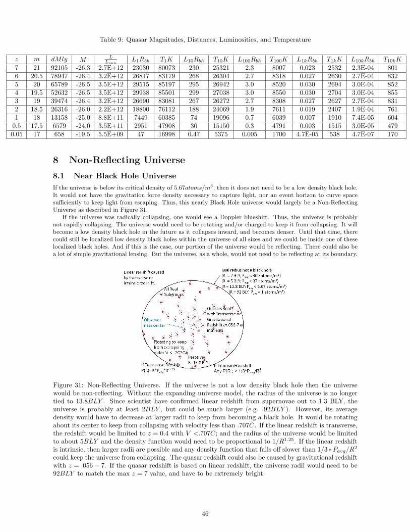
Table 9: Quasar Magnitudes, Distances, Luminosities, and Temperature

z m dMly ML

LsunL1Rbh T1K L10Rbh T10K L100Rbh T100K L1kRbh T1kK L10kRbh T10kK

7 21 92105 -26.3 2.7E+12 23030 80073 230 25321 2.3 8007 0.023 2532 2.3E-04 8016 20.5 78947 -26.4 3.2E+12 26817 83179 268 26304 2.7 8318 0.027 2630 2.7E-04 8325 20 65789 -26.5 3.5E+12 29515 85197 295 26942 3.0 8520 0.030 2694 3.0E-04 8524 19.5 52632 -26.5 3.5E+12 29938 85501 299 27038 3.0 8550 0.030 2704 3.0E-04 8553 19 39474 -26.4 3.2E+12 26690 83081 267 26272 2.7 8308 0.027 2627 2.7E-04 8312 18.5 26316 -26.0 2.2E+12 18800 76112 188 24069 1.9 7611 0.019 2407 1.9E-04 7611 18 13158 -25.0 8.8E+11 7449 60385 74 19096 0.7 6039 0.007 1910 7.4E-05 604

0.5 17.5 6579 -24.0 3.5E+11 2951 47908 30 15150 0.3 4791 0.003 1515 3.0E-05 4790.05 17 658 -19.5 5.5E+09 47 16998 0.47 5375 0.005 1700 4.7E-05 538 4.7E-07 170

8 Non-Reflecting Universe

8.1 Near Black Hole Universe

If the universe is below its critical density of 5.67atoms/m3, then it does not need to be a low density black hole.It would not have the gravitation force density necessary to capture light, nor an event horizon to curve spacesufficiently to keep light from escaping. Thus, this nearly Black Hole universe would largely be a Non-ReflectingUniverse as described in Figure 31.

If the universe was radically collapsing, one would see a Doppler blueshift. Thus, the universe is probablynot rapidly collapsing. The universe would need to be rotating and/or charged to keep it from collapsing. It willbecome a low density black hole in the future as it collapses inward, and becomes denser. Until that time, therecould still be localized low density black holes within the universe of all sizes and we could be inside one of theselocalized black holes. And if this is the case, our portion of the universe would be reflecting. There could also bea lot of simple gravitational lensing. But the universe, as a whole, would not need to be reflecting at its boundary.

Figure 31: Non-Reflecting Universe. If the universe is not a low density black hole then the universewould be non-reflecting. Without the expanding universe model, the radius of the universe is no longertied to 13.8BLY . Since scientist have confirmed linear redshift from supernovae out to 1.3 BLY, theuniverse is probably at least 2BLY , but could be much larger (e.g. 92BLY ). However, its averagedensity would have to decrease at larger radii to keep from becoming a black hole. It would be rotatingabout its center to keep from collapsing with velocity less than .707C. If the linear redshift is transverse,the redshift would be limited to z = 0.4 with V <.707C; and the radius of the universe would be limitedto about 5BLY and the density function would need to be proportional to 1/R1.25. If the linear redshiftis intrinsic, then larger radii are possible and any density function that falls off slower than 1/3∗Pavg/R2

could keep the universe from collapsing. The quasar redshift could also be caused by gravitational redshiftwith z = .056− 7. If the quasar redshift is based on linear redshift, the universe radii would need to be92BLY to match the max z = 7 value, and have to be extremely bright.

46

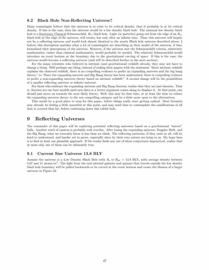
8.2 Black Hole Non-Reflecting Universe?

Many cosmologist believe that the universe is so close to its critical density, that it probably is at its criticaldensity. If this is the case, then the universe would be a low density black hole. The minimal low density blackhole is a Stationary Classical Schwarzschild, Rcs black hole. Light (or particles) going out from the edge of an Rcsblack hole at the edge of the universe, will return, but only after an infinite time. Thus, this universe will largelynot be a reflecting universe and would look almost identical to the nearly Black hole universe described above. Ibelieve this description matches what a lot of cosmologists are describing as their model of the universe, if theyformalized their descriptions of the universe. However, if the universe met the Schwarzschild criteria, relativisticmathematics, rather than classical mathematics, would probably be needed. The relativist Schwarzschild wouldintroduce an event horizon at the boundary due to the gravitational curving of space. If this is the case, theuniverse would become a reflecting universe (and will be described further in the next section).

For the many scientists who believed in intrinsic (and gravitational) redshift already, they may not have tochange a thing. Well perhaps one thing, instead of ending their papers with the statement “Since intrinsic redshiftexplains the observed redshift, there is no compelling evidence to prefer an expanding universe and the big bangtheory.” to “Since the expanding universe and Big Bang theory has been undermined, there is compelling evidenceto prefer a non-expanding universe theory based on intrinsic redshift.” A second change will be the possibilitiesof a smaller reflecting universe or infinite universe.

For those who embrace the expanding universe and Big Bang theories, realize that they are just theories. Thatis, theories are our best models until new data or a better argument comes along to displace it. At that point, oneshould just move on towards the next likely theory. Well, this may be that time, or at least the time to reducethe expanding universe theory to the not compelling category and be a little more open to the alternatives.

This would be a good place to stop for this paper, before things really start getting radical. Most Scientistmay already be feeling a little unsettled at this point, and may need time to contemplate the ramifications of allthat is covered thus far, before continuing down this rabbit hole.

9 Reflecting Universes

The remainder of this paper will be exploring potential reflecting universes based on a gravitational “mirror”balls. Another word of caution is probably well overdue. After losing the expanding universe, Doppler Shift, andthe Big Bang, what we currently know is less than we think. The reflecting universes, if they exist at all, will behard to understand, and harder yet to prove, especially since by their very nature are lying to us. My hope hereis to find at least one plausible approach. If the reader finds any one of these conjectures impractical, realize thatat most only one of them can be ultimately true.

9.1 Current Size Universe 13.8 BLY

Assume the universe is a Low Density Black Hole with Rs or Rbh = 13.8 BLY, with average density between5.67 and 11 atoms/m3. The light from the real internal galaxies and quasars that travels outside the low densityblack hole boundary will be pulled backwards or be curved at the event horizon and create the illusion of a largeruniverse in Figure 32.

47

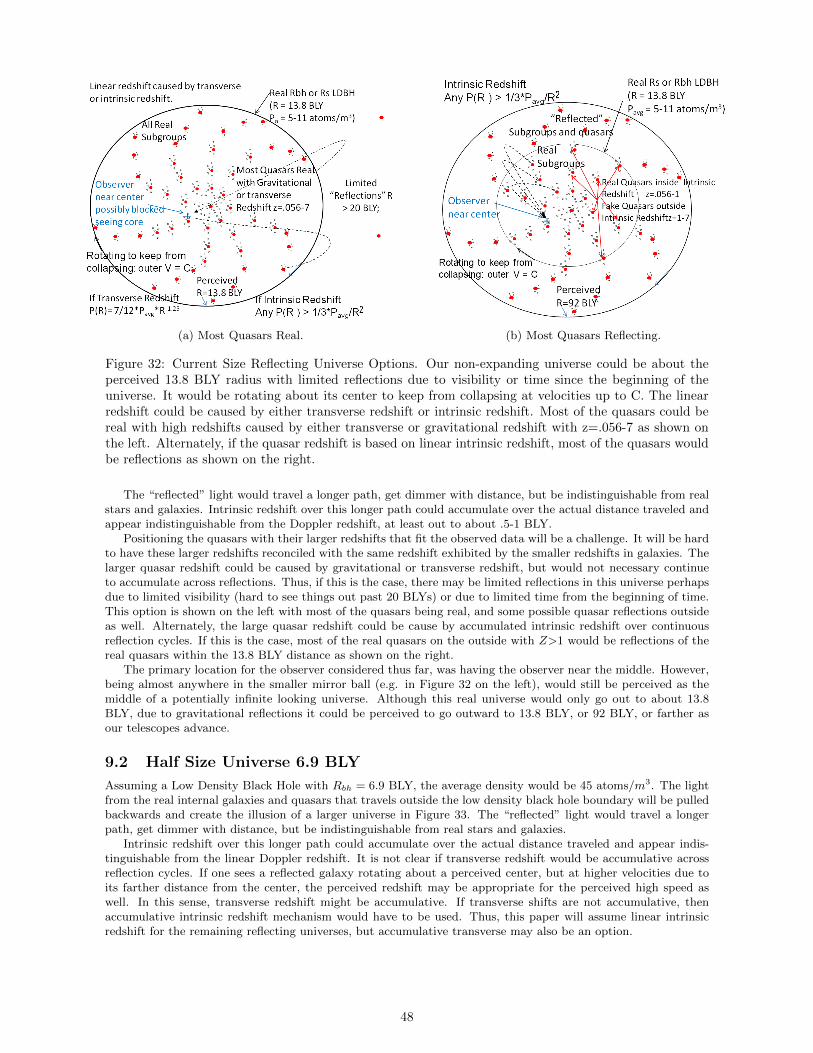
(a) Most Quasars Real. (b) Most Quasars Reflecting.

Figure 32: Current Size Reflecting Universe Options. Our non-expanding universe could be about theperceived 13.8 BLY radius with limited reflections due to visibility or time since the beginning of theuniverse. It would be rotating about its center to keep from collapsing at velocities up to C. The linearredshift could be caused by either transverse redshift or intrinsic redshift. Most of the quasars could bereal with high redshifts caused by either transverse or gravitational redshift with z=.056-7 as shown onthe left. Alternately, if the quasar redshift is based on linear intrinsic redshift, most of the quasars wouldbe reflections as shown on the right.

The “reflected” light would travel a longer path, get dimmer with distance, but be indistinguishable from realstars and galaxies. Intrinsic redshift over this longer path could accumulate over the actual distance traveled andappear indistinguishable from the Doppler redshift, at least out to about .5-1 BLY.

Positioning the quasars with their larger redshifts that fit the observed data will be a challenge. It will be hardto have these larger redshifts reconciled with the same redshift exhibited by the smaller redshifts in galaxies. Thelarger quasar redshift could be caused by gravitational or transverse redshift, but would not necessary continueto accumulate across reflections. Thus, if this is the case, there may be limited reflections in this universe perhapsdue to limited visibility (hard to see things out past 20 BLYs) or due to limited time from the beginning of time.This option is shown on the left with most of the quasars being real, and some possible quasar reflections outsideas well. Alternately, the large quasar redshift could be cause by accumulated intrinsic redshift over continuousreflection cycles. If this is the case, most of the real quasars on the outside with Z>1 would be reflections of thereal quasars within the 13.8 BLY distance as shown on the right.

The primary location for the observer considered thus far, was having the observer near the middle. However,being almost anywhere in the smaller mirror ball (e.g. in Figure 32 on the left), would still be perceived as themiddle of a potentially infinite looking universe. Although this real universe would only go out to about 13.8BLY, due to gravitational reflections it could be perceived to go outward to 13.8 BLY, or 92 BLY, or farther asour telescopes advance.

9.2 Half Size Universe 6.9 BLY

Assuming a Low Density Black Hole with Rbh = 6.9 BLY, the average density would be 45 atoms/m3. The lightfrom the real internal galaxies and quasars that travels outside the low density black hole boundary will be pulledbackwards and create the illusion of a larger universe in Figure 33. The “reflected” light would travel a longerpath, get dimmer with distance, but be indistinguishable from real stars and galaxies.

Intrinsic redshift over this longer path could accumulate over the actual distance traveled and appear indis-tinguishable from the linear Doppler redshift. It is not clear if transverse redshift would be accumulative acrossreflection cycles. If one sees a reflected galaxy rotating about a perceived center, but at higher velocities due toits farther distance from the center, the perceived redshift may be appropriate for the perceived high speed aswell. In this sense, transverse redshift might be accumulative. If transverse shifts are not accumulative, thenaccumulative intrinsic redshift mechanism would have to be used. Thus, this paper will assume linear intrinsicredshift for the remaining reflecting universes, but accumulative transverse may also be an option.

48

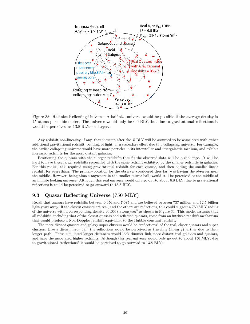
Figure 33: Half size Reflecting Universe. A half size universe would be possible if the average density is45 atoms per cubic meter. The universe would only be 6.9 BLY, but due to gravitational reflections itwould be perceived as 13.8 BLYs or larger.

Any redshift non-linearity, if any, that show up after the .5 BLY will be assumed to be associated with eitheradditional gravitational redshift, bending of light, or a secondary effect due to a collapsing universe. For example,the earlier collapsing universe would have more particles in its interstellar and intergalactic medium, and exhibitincreased redshifts for the most distant galaxies.

Positioning the quasars with their larger redshifts that fit the observed data will be a challenge. It will behard to have these larger redshifts reconciled with the same redshift exhibited by the smaller redshifts in galaxies.For this radius, this required using gravitational redshift for each quasar, and then adding the smaller linearredshift for everything. The primary location for the observer considered thus far, was having the observer nearthe middle. However, being almost anywhere in the smaller mirror ball, would still be perceived as the middle ofan infinite looking universe. Although this real universe would only go out to about 6.8 BLY, due to gravitationalreflections it could be perceived to go outward to 13.8 BLY.

9.3 Quasar Reflecting Universe (750 MLY)

Recall that quasars have redshifts between 0.056 and 7.085 and are believed between 737 million and 12.5 billionlight years away. If the closest quasars are real, and the others are reflections, this could suggest a 750 MLY radiusof the universe with a corresponding density of .0038 atoms/cm3 as shown in Figure 34. This model assumes thatall redshifts, including that of the closest quasars and reflected quasars, come from an intrinsic redshift mechanismthat would produce a Non-Doppler redshift equivalent to the Hubble constant redshift.

The more distant quasars and galaxy super clusters would be “reflections” of the real, closer quasars and superclusters. Like a disco mirror ball, the reflections would be perceived as traveling (linearly) farther due to theirlonger path. These simulated longer distances would look dimmer link more distant real galaxies and quasars,and have the associated higher redshifts. Although this real universe would only go out to about 750 MLY, dueto gravitational “reflections” it would be perceived to go outward to 13.8 BLYs.

49

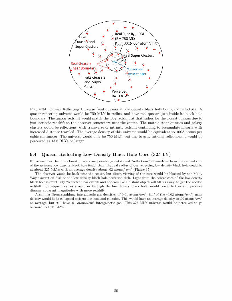
Figure 34: Quasar Reflecting Universe (real quasars at low density black hole boundary reflected). Aquasar reflecting universe would be 750 MLY in radius, and have real quasars just inside its black holeboundary. The quasar redshift would match the .062 redshift at that radius for the closest quasars due tojust intrinsic redshift to the observer somewhere near the center. The more distant quasars and galaxyclusters would be reflections, with transverse or intrinsic redshift continuing to accumulate linearly withincreased distance traveled. The average density of this universe would be equivalent to .0038 atoms percubic centimeter. The universe would only be 750 MLY, but due to gravitational reflections it would beperceived as 13.8 BLYs or larger.

9.4 Quasar Reflecting Low Density Black Hole Core (325 LY)

If one assumes that the closest quasars are possible gravitational “reflections” themselves, from the central coreof the universe low density black hole itself; then, the real radius of our reflecting low density black hole could beat about 325 MLYs with an average density about .02 atoms/ cm3 (Figure 35).

The observer would be back near the center, but direct viewing of the core would be blocked by the MilkyWay’s accretion disk or the low density black hole accretion disk. Light from the center core of the low densityblack hole is eventually “reflected” backwards and appears like a distant object 750 MLYs away, to get the neededredshift. Subsequent cycles around or through the low density black hole, would travel farther and producedimmer apparent magnitudes with more redshift.

Assuming Bremsstrahlung intergalactic gas densities of 0.01 atoms/cm3, half of the (0.02 atoms/cm3) massdensity would be in collapsed objects like suns and galaxies. This would have an average density to .02 atoms/cm3

on average, but still have .01 atoms/cm3 intergalactic gas. This 325 MLY universe would be perceived to gooutward to 13.8 BLYs.

50

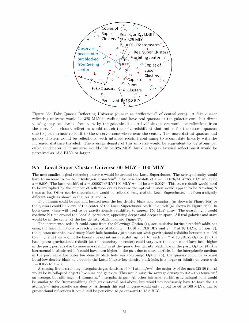
Figure 35: Fake Quasar Reflecting Universe (quasar as “reflections” of central core). A fake quasarreflecting universe would be 325 MLY in radius, and have real quasars at the galactic core, but directviewing may be blocked from view by the galactic disk. All visible quasars would be reflections fromthe core. The closest reflection would match the .062 redshift at that radius for the closest quasarsdue to just intrinsic redshift to the observer somewhere near the center. The more distant quasars andgalaxy clusters would be reflections, with intrinsic redshift continuing to accumulate linearly with theincreased distance traveled. The average density of this universe would be equivalent to .02 atoms percubic centimeter. The universe would only be 325 MLY, but due to gravitational reflections it would beperceived as 13.8 BLYs or larger.

9.5 Local Super Cluster Universe 66 MLY - 100 MLY

The next smaller logical reflecting universe would be around the Local Supercluster. The average density wouldhave to increase to .25 to .5 hydrogen atoms/cm3. The base redshift of z = .000076/MLY*66 MLY would bez = 0.005. The base redshift of z = .000076/MLY*100 MLY would be z = 0.0076. This base redshift would needto be multiplied by the number of reflection cycles because the optical illusion would appear to be traveling Ntimes as far. Other nearby superclusters would be reflected images of the Local Supercluster, but from a slightlydifferent angle as shown in Figures 36 and 37.

The quasars could be real and located near the low density black hole boundary (as shown in Figure 36a) orthe quasars could be views of the center of the Local Supercluster black hole itself (as shown in Figure 36b). Inboth cases, these will need to be gravitationally redshifted to appear 750 MLY away. The quasar light wouldcontinue N time around the Local Supercluster, appearing deeper and deeper in space. All real galaxies and starswould be in the center of the low density black hole, see Figure 37.

The incremental redshift could come from the following: Option (1), accumulative intrinsic redshift additionsusing the linear functions to reach z values of about z = 1.056 at 13.8 BLY and z = 7 at 92 BLYs; Option (2),the quasars near the low density black hole boundary just start out with gravitational redshifts between z = .056to z = 6; and then adding the linearly based intrinsic redshift up to 1 to reach z = 7 at 13.8BLY; Option (3), thebase quasar gravitational redshift (at the boundary or center) could vary over time and could have been higherin the past, perhaps due to more mass falling in at the quasar low density black hole in the past; Option (4), theincremental intrinsic redshift could have been higher in the past due to more particles in the intergalactic mediumin the past while the outer low density black hole was collapsing; Option (5), the quasars could be externalLocal low density black hole outside the Local Cluster low density black hole, in a larger or infinite universe withz = 0.056 to z = 7.

Assuming Bremsstrahlung intergalactic gas densities of 0.01 atoms/cm3, the majority of the mass (25-50 times)would be in collapsed objects like suns and galaxies. This would raise the average density to 0.25-0.5 atoms/cm3

on average, but still have .01 atoms/cm3 intergalactic gas. All other intrinsic redshift gravitational balls wouldbe similar to the Bremsstrahlung shift gravitational ball above, but would not necessarily have to have the .01atoms/cm3 intergalactic gas density. Although this real universe would only go out to 66 to 100 MLYs, due togravitational reflections it could still be perceived to go outward to 13.8 BLY.

51

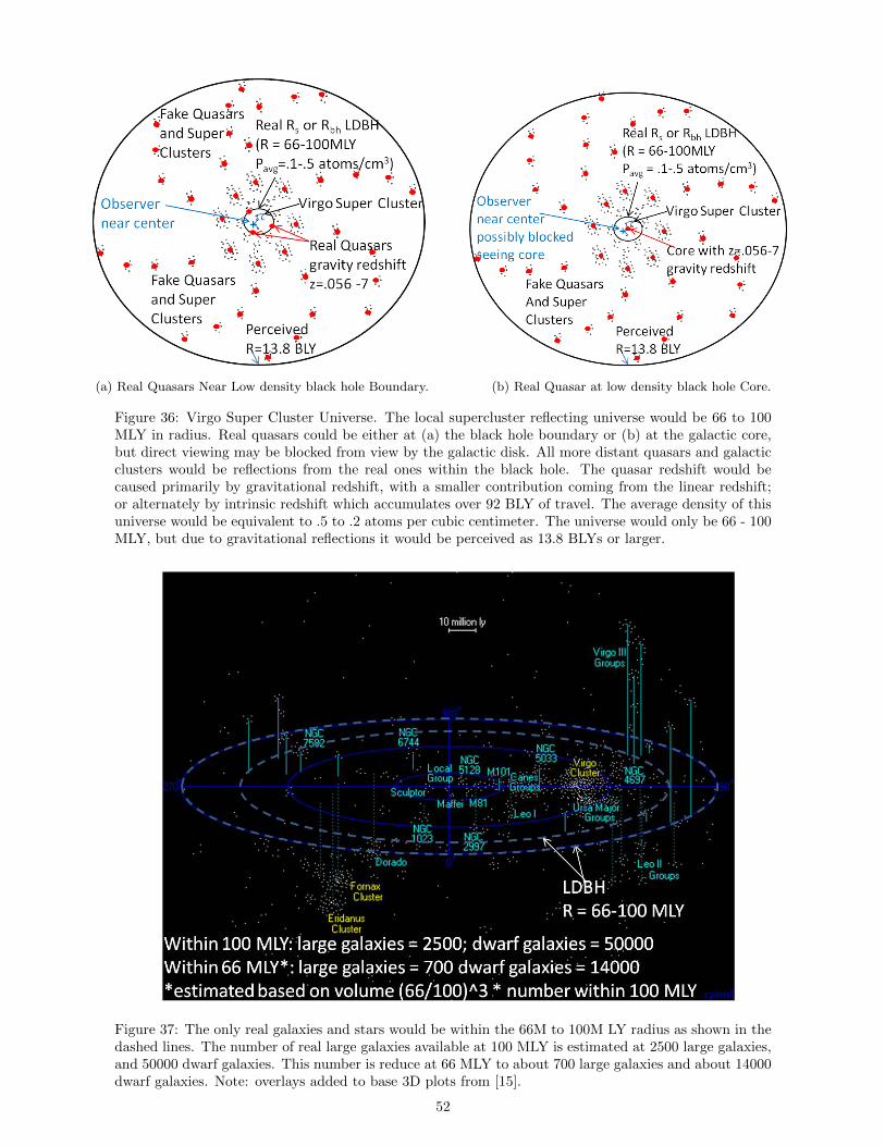
(a) Real Quasars Near Low density black hole Boundary. (b) Real Quasar at low density black hole Core.

Figure 36: Virgo Super Cluster Universe. The local supercluster reflecting universe would be 66 to 100MLY in radius. Real quasars could be either at (a) the black hole boundary or (b) at the galactic core,but direct viewing may be blocked from view by the galactic disk. All more distant quasars and galacticclusters would be reflections from the real ones within the black hole. The quasar redshift would becaused primarily by gravitational redshift, with a smaller contribution coming from the linear redshift;or alternately by intrinsic redshift which accumulates over 92 BLY of travel. The average density of thisuniverse would be equivalent to .5 to .2 atoms per cubic centimeter. The universe would only be 66 - 100MLY, but due to gravitational reflections it would be perceived as 13.8 BLYs or larger.

Figure 37: The only real galaxies and stars would be within the 66M to 100M LY radius as shown in thedashed lines. The number of real large galaxies available at 100 MLY is estimated at 2500 large galaxies,and 50000 dwarf galaxies. This number is reduce at 66 MLY to about 700 large galaxies and about 14000dwarf galaxies. Note: overlays added to base 3D plots from [15].

52

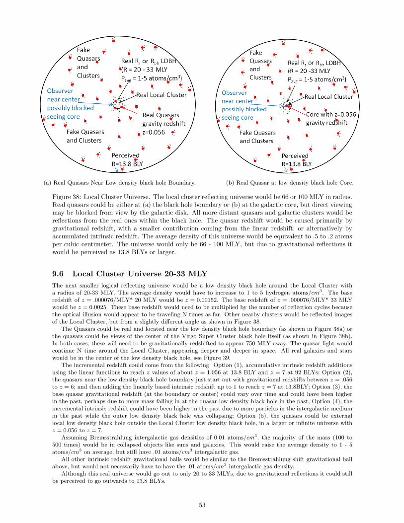
(a) Real Quasars Near Low density black hole Boundary. (b) Real Quasar at low density black hole Core.

Figure 38: Local Cluster Universe. The local cluster reflecting universe would be 66 or 100 MLY in radius.Real quasars could be either at (a) the black hole boundary or (b) at the galactic core, but direct viewingmay be blocked from view by the galactic disk. All more distant quasars and galactic clusters would bereflections from the real ones within the black hole. The quasar redshift would be caused primarily bygravitational redshift, with a smaller contribution coming from the linear redshift; or alternatively byaccumulated intrinsic redshift. The average density of this universe would be equivalent to .5 to .2 atomsper cubic centimeter. The universe would only be 66 - 100 MLY, but due to gravitational reflections itwould be perceived as 13.8 BLYs or larger.

9.6 Local Cluster Universe 20-33 MLY

The next smaller logical reflecting universe would be a low density black hole around the Local Cluster witha radius of 20-33 MLY. The average density would have to increase to 1 to 5 hydrogen atoms/cm3. The baseredshift of z = .000076/MLY* 20 MLY would be z = 0.00152. The base redshift of z = .000076/MLY* 33 MLYwould be z = 0.0025. These base redshift would need to be multiplied by the number of reflection cycles becausethe optical illusion would appear to be traveling N times as far. Other nearby clusters would be reflected imagesof the Local Cluster, but from a slightly different angle as shown in Figure 38.

The Quasars could be real and located near the low density black hole boundary (as shown in Figure 38a) orthe quasars could be views of the center of the Virgo Super Cluster black hole itself (as shown in Figure 38b).In both cases, these will need to be gravitationally redshifted to appear 750 MLY away. The quasar light wouldcontinue N time around the Local Cluster, appearing deeper and deeper in space. All real galaxies and starswould be in the center of the low density black hole, see Figure 39.

The incremental redshift could come from the following: Option (1), accumulative intrinsic redshift additionsusing the linear functions to reach z values of about z = 1.056 at 13.8 BLY and z = 7 at 92 BLYs; Option (2),the quasars near the low density black hole boundary just start out with gravitational redshifts between z = .056to z = 6; and then adding the linearly based intrinsic redshift up to 1 to reach z = 7 at 13.8BLY; Option (3), thebase quasar gravitational redshift (at the boundary or center) could vary over time and could have been higherin the past, perhaps due to more mass falling in at the quasar low density black hole in the past; Option (4), theincremental intrinsic redshift could have been higher in the past due to more particles in the intergalactic mediumin the past while the outer low density black hole was collapsing; Option (5), the quasars could be externallocal low density black hole outside the Local Cluster low density black hole, in a larger or infinite universe withz = 0.056 to z = 7.

Assuming Bremsstrahlung intergalactic gas densities of 0.01 atoms/cm3, the majority of the mass (100 to500 times) would be in collapsed objects like suns and galaxies. This would raise the average density to 1 - 5atoms/cm3 on average, but still have .01 atoms/cm3 intergalactic gas.

All other intrinsic redshift gravitational balls would be similar to the Bremsstrahlung shift gravitational ballabove, but would not necessarily have to have the .01 atoms/cm3 intergalactic gas density.

Although this real universe would go out to only 20 to 33 MLYs, due to gravitational reflections it could stillbe perceived to go outwards to 13.8 BLYs.

53

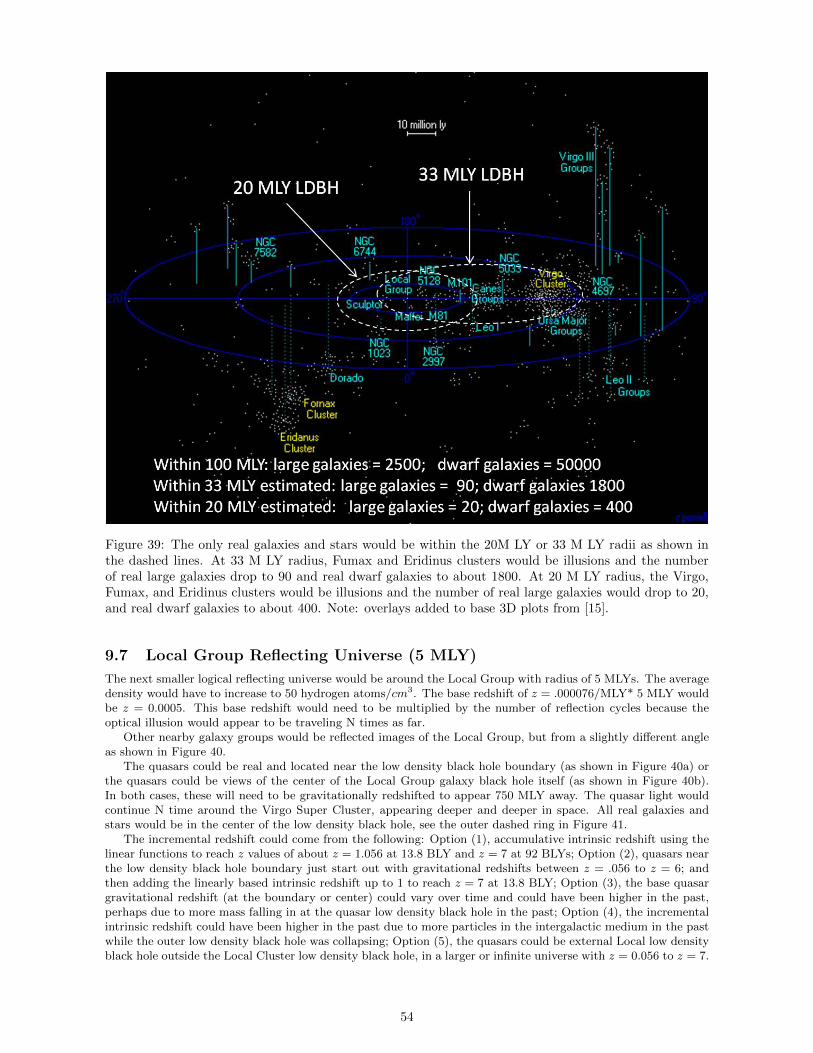
Figure 39: The only real galaxies and stars would be within the 20M LY or 33 M LY radii as shown inthe dashed lines. At 33 M LY radius, Fumax and Eridinus clusters would be illusions and the numberof real large galaxies drop to 90 and real dwarf galaxies to about 1800. At 20 M LY radius, the Virgo,Fumax, and Eridinus clusters would be illusions and the number of real large galaxies would drop to 20,and real dwarf galaxies to about 400. Note: overlays added to base 3D plots from [15].

9.7 Local Group Reflecting Universe (5 MLY)

The next smaller logical reflecting universe would be around the Local Group with radius of 5 MLYs. The averagedensity would have to increase to 50 hydrogen atoms/cm3. The base redshift of z = .000076/MLY* 5 MLY wouldbe z = 0.0005. This base redshift would need to be multiplied by the number of reflection cycles because theoptical illusion would appear to be traveling N times as far.

Other nearby galaxy groups would be reflected images of the Local Group, but from a slightly different angleas shown in Figure 40.

The quasars could be real and located near the low density black hole boundary (as shown in Figure 40a) orthe quasars could be views of the center of the Local Group galaxy black hole itself (as shown in Figure 40b).In both cases, these will need to be gravitationally redshifted to appear 750 MLY away. The quasar light wouldcontinue N time around the Virgo Super Cluster, appearing deeper and deeper in space. All real galaxies andstars would be in the center of the low density black hole, see the outer dashed ring in Figure 41.

The incremental redshift could come from the following: Option (1), accumulative intrinsic redshift using thelinear functions to reach z values of about z = 1.056 at 13.8 BLY and z = 7 at 92 BLYs; Option (2), quasars nearthe low density black hole boundary just start out with gravitational redshifts between z = .056 to z = 6; andthen adding the linearly based intrinsic redshift up to 1 to reach z = 7 at 13.8 BLY; Option (3), the base quasargravitational redshift (at the boundary or center) could vary over time and could have been higher in the past,perhaps due to more mass falling in at the quasar low density black hole in the past; Option (4), the incrementalintrinsic redshift could have been higher in the past due to more particles in the intergalactic medium in the pastwhile the outer low density black hole was collapsing; Option (5), the quasars could be external Local low densityblack hole outside the Local Cluster low density black hole, in a larger or infinite universe with z = 0.056 to z = 7.

54

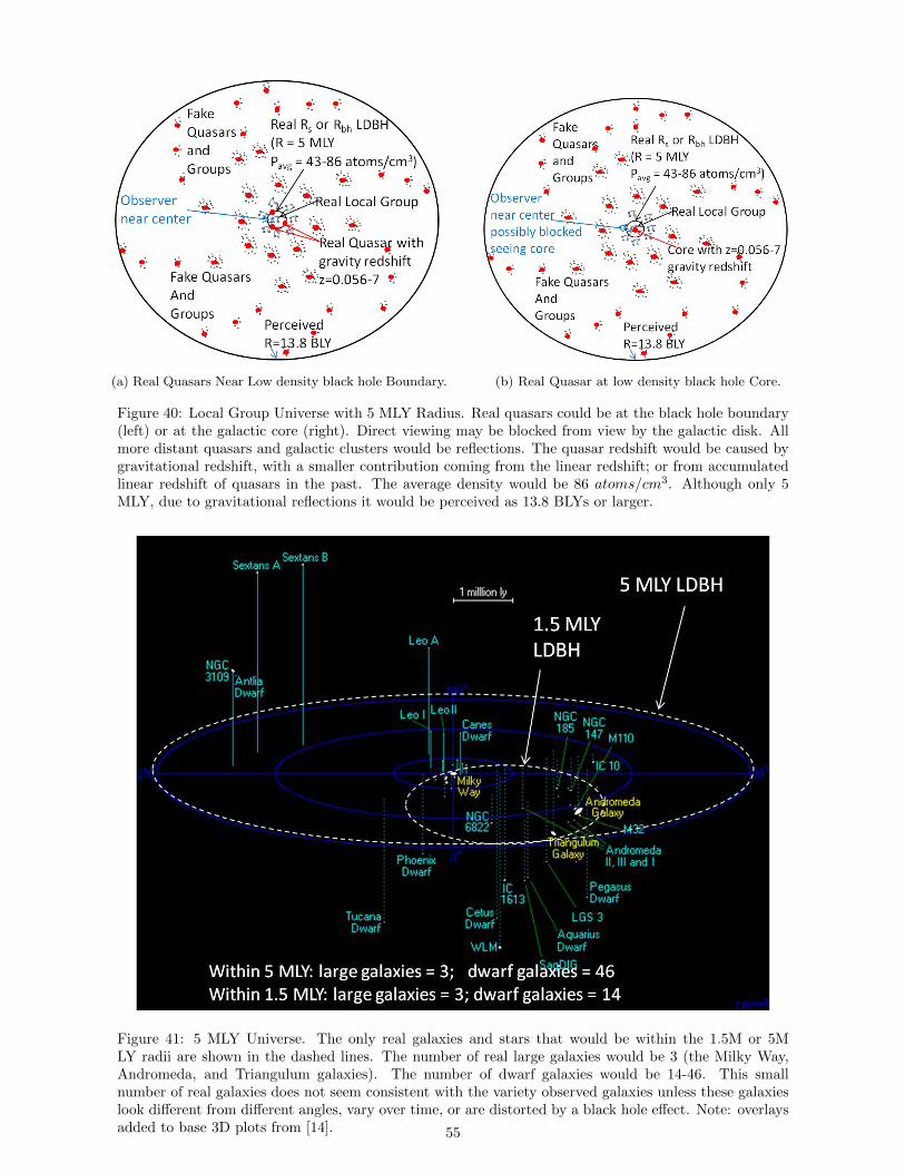
(a) Real Quasars Near Low density black hole Boundary. (b) Real Quasar at low density black hole Core.

Figure 40: Local Group Universe with 5 MLY Radius. Real quasars could be at the black hole boundary(left) or at the galactic core (right). Direct viewing may be blocked from view by the galactic disk. Allmore distant quasars and galactic clusters would be reflections. The quasar redshift would be caused bygravitational redshift, with a smaller contribution coming from the linear redshift; or from accumulatedlinear redshift of quasars in the past. The average density would be 86 atoms/cm3. Although only 5MLY, due to gravitational reflections it would be perceived as 13.8 BLYs or larger.

Figure 41: 5 MLY Universe. The only real galaxies and stars that would be within the 1.5M or 5MLY radii are shown in the dashed lines. The number of real large galaxies would be 3 (the Milky Way,Andromeda, and Triangulum galaxies). The number of dwarf galaxies would be 14-46. This smallnumber of real galaxies does not seem consistent with the variety observed galaxies unless these galaxieslook different from different angles, vary over time, or are distorted by a black hole effect. Note: overlaysadded to base 3D plots from [14]. 55

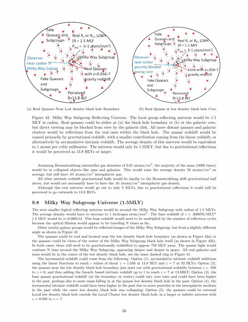
(a) Real Quasars Near Low density black hole Boundary. (b) Real Quasar at low density black hole Core.

Figure 42: Milky Way Subgroup Reflecting Universe. The local group reflecting universe would be 1.5MLY in radius. Real quasars could be either at (a) the black hole boundary or (b) at the galactic core,but direct viewing may be blocked from view by the galactic disk. All more distant quasars and galacticclusters would be reflections from the real ones within the black hole. The quasar redshift would becaused primarily by gravitational redshift, with a smaller contribution coming from the linear redshift; oralternatively by accumulative intrinsic redshift. The average density of this universe would be equivalentto 1 atoms per cubic millimeter. The universe would only be 1.5MLY, but due to gravitational reflectionsit would be perceived as 13.8 BLYs or larger.

Assuming Bremsstrahlung interstellar gas densities of 0.01 atoms/cm3, the majority of the mass (5000 times)would be in collapsed objects like suns and galaxies. This would raise the average density 50 atoms/cm3 onaverage, but still have .01 atoms/cm3 intergalactic gas.

All other intrinsic redshift gravitational balls would be similar to the Bremsstrahlung shift gravitational ballabove, but would not necessarily have to have the .01 atoms/cm3 intergalactic gas density.

Although this real universe would go out to only 5 MLYs, due to gravitational reflections it could still beperceived to go outwards to 13.8 BLYs.

9.8 Milky Way Subgroup Universe (1.5MLY)

The next smaller logical reflecting universe would be around the Milky Way Subgroup with radius of 1.5 MLYs.The average density would have to increase to 1 hydrogen atom/mm3. The base redshift of z = .000076/MLY*1.5 MLY would be z=0.000114. This base redshift would need to be multiplied by the number of reflection cyclesbecause the optical illusion would appear to be traveling N times as far.

Other nearby galaxy groups would be reflected images of the Milky Way Subgroup, but from a slightly differentangle as shown in Figure 42.

The quasars could be real and located near the low density black hole boundary (as shown in Figure 42a) orthe quasars could be views of the center of the Milky Way Subgroup black hole itself (as shown in Figure 42b).In both cases, these will need to be gravitationally redshifted to appear 750 MLY away. The quasar light wouldcontinue N time around the Milky Way Subgroup, appearing deeper and deeper in space. All real galaxies andstars would be in the center of the low density black hole, see the inner dashed ring in Figure 41.

The incremental redshift could come from the following: Option (1), accumulative intrinsic redshift additionsusing the linear functions to reach z values of about z = 1.056 at 13.8 BLY and z = 7 at 92 BLYs; Option (2),the quasars near the low density black hole boundary just start out with gravitational redshifts between z = .056to z = 6; and then adding the linearly based intrinsic redshift up to 1 to reach z = 7 at 13.8BLY; Option (3), thebase quasar gravitational redshift (at the boundary or center) could vary over time and could have been higherin the past, perhaps due to more mass falling in at the quasar low density black hole in the past; Option (4), theincremental intrinsic redshift could have been higher in the past due to more particles in the intergalactic mediumin the past while the outer low density black hole was collapsing; Option (5), the quasars could be externalLocal low density black hole outside the Local Cluster low density black hole, in a larger or infinite universe withz = 0.056 to z = 7.

56

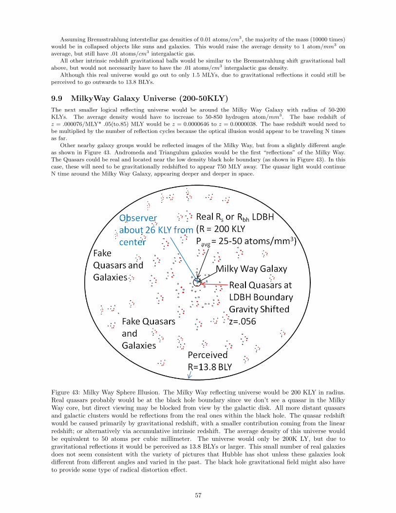
Assuming Bremsstrahlung interstellar gas densities of 0.01 atoms/cm3, the majority of the mass (10000 times)would be in collapsed objects like suns and galaxies. This would raise the average density to 1 atom/mm3 onaverage, but still have .01 atoms/cm3 intergalactic gas.

All other intrinsic redshift gravitational balls would be similar to the Bremsstrahlung shift gravitational ballabove, but would not necessarily have to have the .01 atoms/cm3 intergalactic gas density.

Although this real universe would go out to only 1.5 MLYs, due to gravitational reflections it could still beperceived to go outwards to 13.8 BLYs.

9.9 MilkyWay Galaxy Universe (200-50KLY)

The next smaller logical reflecting universe would be around the Milky Way Galaxy with radius of 50-200KLYs. The average density would have to increase to 50-850 hydrogen atom/mm3. The base redshift ofz = .000076/MLY* .05(to.85) MLY would be z = 0.0000646 to z = 0.0000038. The base redshift would need tobe multiplied by the number of reflection cycles because the optical illusion would appear to be traveling N timesas far.

Other nearby galaxy groups would be reflected images of the Milky Way, but from a slightly different angleas shown in Figure 43. Andromeda and Triangulum galaxies would be the first “reflections” of the Milky Way.The Quasars could be real and located near the low density black hole boundary (as shown in Figure 43). In thiscase, these will need to be gravitationally redshifted to appear 750 MLY away. The quasar light would continueN time around the Milky Way Galaxy, appearing deeper and deeper in space.

Figure 43: Milky Way Sphere Illusion. The Milky Way reflecting universe would be 200 KLY in radius.Real quasars probably would be at the black hole boundary since we don’t see a quasar in the MilkyWay core, but direct viewing may be blocked from view by the galactic disk. All more distant quasarsand galactic clusters would be reflections from the real ones within the black hole. The quasar redshiftwould be caused primarily by gravitational redshift, with a smaller contribution coming from the linearredshift; or alternatively via accumulative intrinsic redshift. The average density of this universe wouldbe equivalent to 50 atoms per cubic millimeter. The universe would only be 200K LY, but due togravitational reflections it would be perceived as 13.8 BLYs or larger. This small number of real galaxiesdoes not seem consistent with the variety of pictures that Hubble has shot unless these galaxies lookdifferent from different angles and varied in the past. The black hole gravitational field might also haveto provide some type of radical distortion effect.

57

The incremental redshift could come from the following: Option (1), accumulative intrinsic redshift additionsusing the linear functions to reach z values of about z = 1.056 at 13.8 BLY and z = 7 at 92 BLYs; Option (2),the quasars near the low density black hole boundary just start out with gravitational redshifts between z = .056to z = 6; and then adding the linearly based intrinsic redshift up to 1 to reach z = 7 at 13.8BLY; Option (3), thebase quasar gravitational redshift (at the boundary or center) could vary over time and could have been higherin the past, perhaps due to more mass falling in at the quasar low density black hole in the past; Option (4), theincremental intrinsic redshift could have been higher in the past due to more particles in the intergalactic mediumin the past while the outer low density black hole was collapsing; Option (5), the quasars could be externalLocal low density black hole outside the Local Cluster low density black hole, in a larger or infinite universe withz = 0.056 to z = 7.

Assuming Bremsstrahlung interstellar gas densities of 0.01 atoms/cm3, the majority of the mass (50000-850000 times) would be in collapsed mass like suns and galaxies. This would raise the average density to 50-850atoms/mm3 on average, but still have .01 atoms/cm3 intergalactic gas.

All other intrinsic redshift gravitational balls would be similar to the Bremsstrahlung shift gravitational ballabove, but would not necessarily have to have the .01 atoms/cm3 intergalactic gas density.

Although this real universe would go out to only 200-50 KLYs, due to gravitational reflections it could still beperceived to go outwards to 13.8 BLYs

9.10 Sub Galaxy universe (e.g.< 50 KLY)

The average density would have to increase further to produce a low density black hole at smaller than the galaxyboundaries. The rotating low density black hole would then have to also create the illusion of a full galaxy(perhaps by frame dragging space in a spiral pattern). Then it would have to multiply this galaxy image via themirrored ball or gravitational redshifting, and have them look different from different angles.

10 Quantized redshift

These last two Milky Way Subgroup and Galaxy low density black holes would actually fit the quantized galacticdistances and quantized redshift phenomenon researched in the late 90s [47, 48, 49, 50, 51]. Other scientists(including Hawking) tried to find this periodicity with the latest data but found no correlation, or that could notbe explained by grouping or selection effects [47]. It also seemed to disagree with the Big Bang universe at thetime. Maybe with the Big Bang Theory off the table, quantized redshifts might warrant a second look.

Note that the primary source of the redshift quantization presented here is from the reflected galaxies comingin reflective waves at periodic radii, and thus, there would be more redshift at these radii and less (or none) atothers. There may also be some minor secondary affects due to variations in the source of the redshift outside theblack hole or at its boundary. Also note, the reflecting universes presented earlier do not depend on this quantizedredshift. But if quantized redshift is present, a reflecting black hole could be its source. Additionally, the lowdensity black holes are not like stellar black holes containing only one light source, but are very large with manygalaxies at different depths. Thus, the light can start reflecting at lower levels and travel in arbitrary arcs. Thus,crisp distinctive quantized levels may not be blatantly observable, but may only show up statistically.

10.1 Milk Way Group Quantized Universe

Tifft and colleagues found periodic quantized redshifts in nearby galaxies data in primary increments aroundz = .00024 and z = .00012 with minor sub-harmonics at z = .00008 (Doppler velocities of 72, 36, and 24 km/s)and that nearby galaxies were spaced in periodic intervals of about 3 MLY.

In 1997, Napier and Guthrie performed an independent redshift analysis of nearby galaxies and found aperiodicity at 38 km/sec as shown in Figure 44 from Napier et al. [52]. Napier’s and Guthrie’s final statement:“Our conclusion is that extragalactic redshifts are quantized along the lines originally suggested by Tifft andcoworkers, with galacto-centric periodicities of 37.5 km/sec in field galaxies and loose groupings, and 71.1 km/secin the environment of dense clusters.”

58

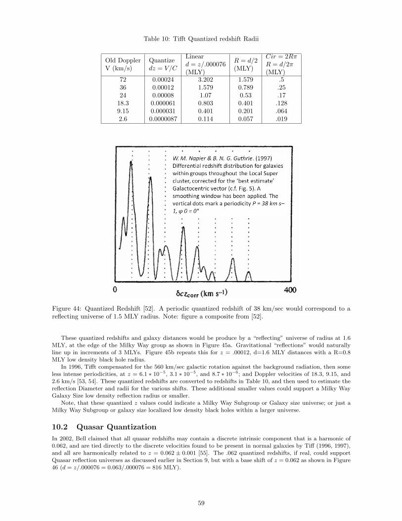
Table 10: Tifft Quantized redshift Radii

Old DopplerV (km/s)

Quantizedz = V/C

Lineard = z/.000076(MLY)

R = d/2(MLY)

Cir = 2RπR = d/2π(MLY)

72 0.00024 3.202 1.579 .536 0.00012 1.579 0.789 .2524 0.00008 1.07 0.53 .17

18.3 0.000061 0.803 0.401 .1289.15 0.000031 0.401 0.201 .0642.6 0.0000087 0.114 0.057 .019

Figure 44: Quantized Redshift [52]. A periodic quantized redshift of 38 km/sec would correspond to areflecting universe of 1.5 MLY radius. Note: figure a composite from [52].

These quantized redshifts and galaxy distances would be produce by a “reflecting” universe of radius at 1.6MLY, at the edge of the Milky Way group as shown in Figure 45a. Gravitational “reflections” would naturallyline up in increments of 3 MLYs. Figure 45b repeats this for z = .00012, d=1.6 MLY distances with a R=0.8MLY low density black hole radius.

In 1996, Tifft compensated for the 560 km/sec galactic rotation against the background radiation, then someless intense periodicities, at z = 6.1 ∗ 10−5, 3.1 ∗ 10−5, and 8.7 ∗ 10−6; and Doppler velocities of 18.3, 9.15, and2.6 km/s [53, 54]. These quantized redshifts are converted to redshifts in Table 10, and then used to estimate thereflection Diameter and radii for the various shifts. These additional smaller values could support a Milky WayGalaxy Size low density reflection radius or smaller.

Note, that these quantized z values could indicate a Milky Way Subgroup or Galaxy size universe; or just aMilky Way Subgroup or galaxy size localized low density black holes within a larger universe.

10.2 Quasar Quantization

In 2002, Bell claimed that all quasar redshifts may contain a discrete intrinsic component that is a harmonic of0.062, and are tied directly to the discrete velocities found to be present in normal galaxies by Tiff (1996, 1997),and all are harmonically related to z = 0.062 ± 0.001 [55]. The .062 quantized redshifts, if real, could supportQuasar reflection universes as discussed earlier in Section 9, but with a base shift of z = 0.062 as shown in Figure46 (d = z/.000076 = 0.063/.000076 = 816 MLY).

59

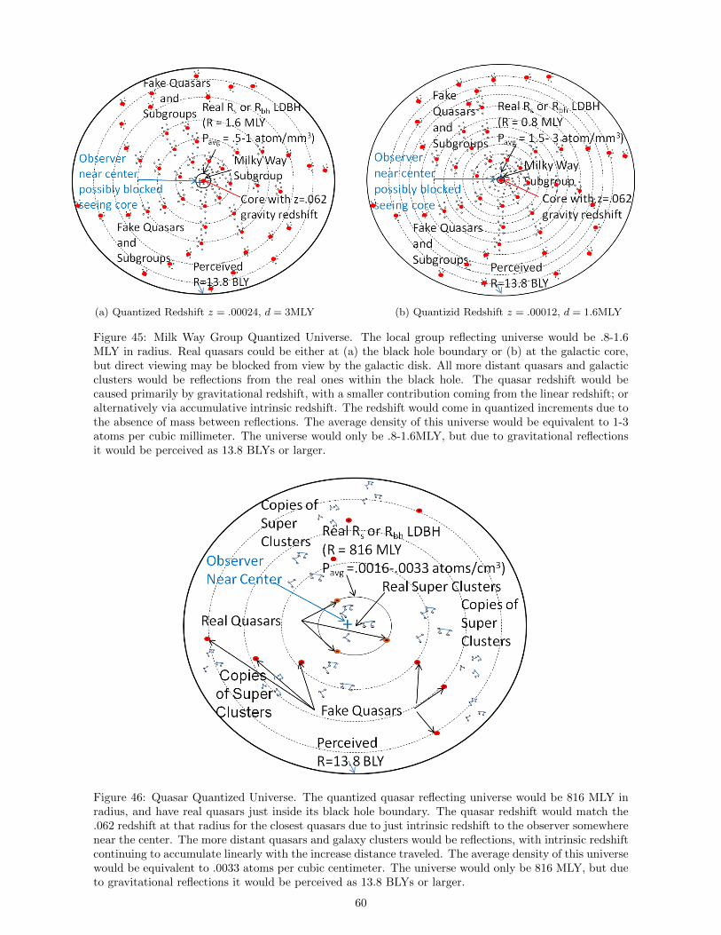
(a) Quantized Redshift z = .00024, d = 3MLY (b) Quantizid Redshift z = .00012, d = 1.6MLY

Figure 45: Milk Way Group Quantized Universe. The local group reflecting universe would be .8-1.6MLY in radius. Real quasars could be either at (a) the black hole boundary or (b) at the galactic core,but direct viewing may be blocked from view by the galactic disk. All more distant quasars and galacticclusters would be reflections from the real ones within the black hole. The quasar redshift would becaused primarily by gravitational redshift, with a smaller contribution coming from the linear redshift; oralternatively via accumulative intrinsic redshift. The redshift would come in quantized increments due tothe absence of mass between reflections. The average density of this universe would be equivalent to 1-3atoms per cubic millimeter. The universe would only be .8-1.6MLY, but due to gravitational reflectionsit would be perceived as 13.8 BLYs or larger.

Figure 46: Quasar Quantized Universe. The quantized quasar reflecting universe would be 816 MLY inradius, and have real quasars just inside its black hole boundary. The quasar redshift would match the.062 redshift at that radius for the closest quasars due to just intrinsic redshift to the observer somewherenear the center. The more distant quasars and galaxy clusters would be reflections, with intrinsic redshiftcontinuing to accumulate linearly with the increase distance traveled. The average density of this universewould be equivalent to .0033 atoms per cubic centimeter. The universe would only be 816 MLY, but dueto gravitational reflections it would be perceived as 13.8 BLYs or larger.

60

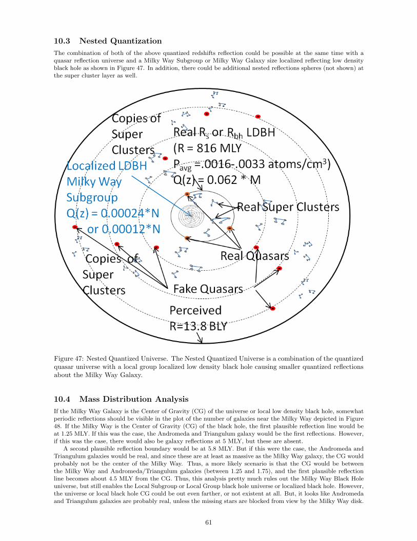
10.3 Nested Quantization

The combination of both of the above quantized redshifts reflection could be possible at the same time with aquasar reflection universe and a Milky Way Subgroup or Milky Way Galaxy size localized reflecting low densityblack hole as shown in Figure 47. In addition, there could be additional nested reflections spheres (not shown) atthe super cluster layer as well.

Figure 47: Nested Quantized Universe. The Nested Quantized Universe is a combination of the quantizedquasar universe with a local group localized low density black hole causing smaller quantized reflectionsabout the Milky Way Galaxy.

10.4 Mass Distribution Analysis

If the Milky Way Galaxy is the Center of Gravity (CG) of the universe or local low density black hole, somewhatperiodic reflections should be visible in the plot of the number of galaxies near the Milky Way depicted in Figure48. If the Milky Way is the Center of Gravity (CG) of the black hole, the first plausible reflection line would beat 1.25 MLY. If this was the case, the Andromeda and Triangulum galaxy would be the first reflections. However,if this was the case, there would also be galaxy reflections at 5 MLY, but these are absent.

A second plausible reflection boundary would be at 5.8 MLY. But if this were the case, the Andromeda andTriangulum galaxies would be real, and since these are at least as massive as the Milky Way galaxy, the CG wouldprobably not be the center of the Milky Way. Thus, a more likely scenario is that the CG would be betweenthe Milky Way and Andromeda/Triangulum galaxies (between 1.25 and 1.75), and the first plausible reflectionline becomes about 4.5 MLY from the CG. Thus, this analysis pretty much rules out the Milky Way Black Holeuniverse, but still enables the Local Subgroup or Local Group black hole universe or localized black hole. However,the universe or local black hole CG could be out even farther, or not existent at all. But, it looks like Andromedaand Triangulum galaxies are probably real, unless the missing stars are blocked from view by the Milky Way disk.

61

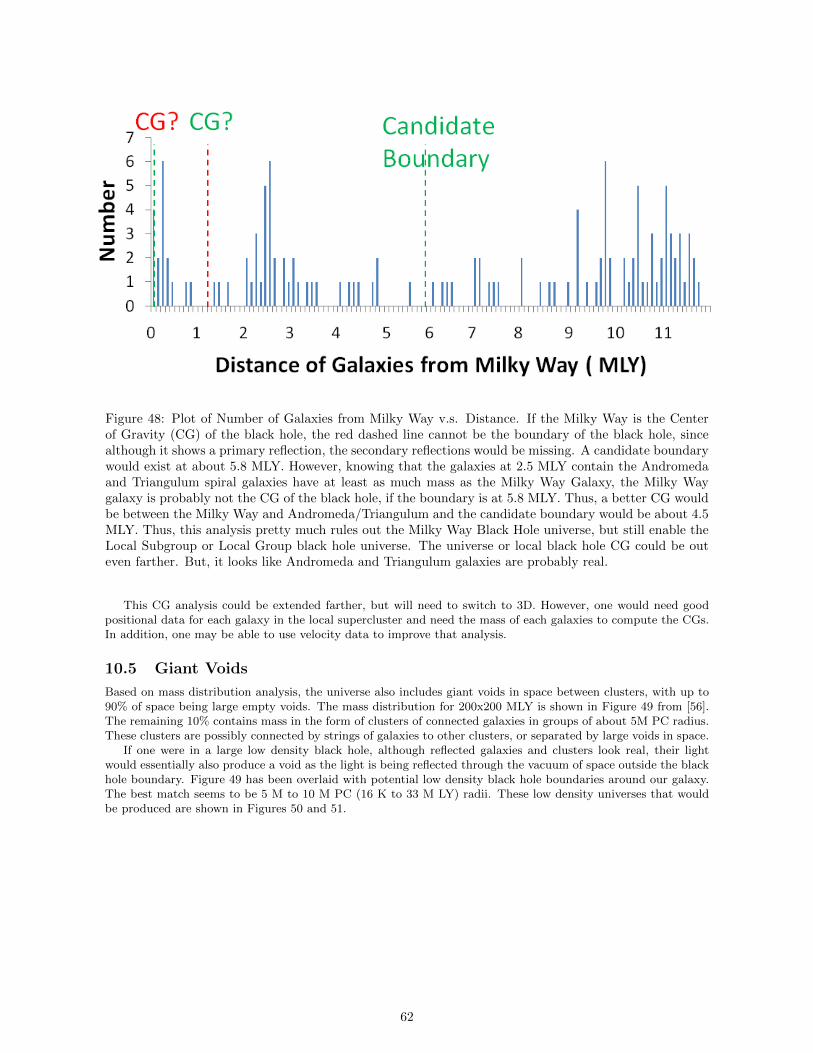
Figure 48: Plot of Number of Galaxies from Milky Way v.s. Distance. If the Milky Way is the Centerof Gravity (CG) of the black hole, the red dashed line cannot be the boundary of the black hole, sincealthough it shows a primary reflection, the secondary reflections would be missing. A candidate boundarywould exist at about 5.8 MLY. However, knowing that the galaxies at 2.5 MLY contain the Andromedaand Triangulum spiral galaxies have at least as much mass as the Milky Way Galaxy, the Milky Waygalaxy is probably not the CG of the black hole, if the boundary is at 5.8 MLY. Thus, a better CG wouldbe between the Milky Way and Andromeda/Triangulum and the candidate boundary would be about 4.5MLY. Thus, this analysis pretty much rules out the Milky Way Black Hole universe, but still enable theLocal Subgroup or Local Group black hole universe. The universe or local black hole CG could be outeven farther. But, it looks like Andromeda and Triangulum galaxies are probably real.

This CG analysis could be extended farther, but will need to switch to 3D. However, one would need goodpositional data for each galaxy in the local supercluster and need the mass of each galaxies to compute the CGs.In addition, one may be able to use velocity data to improve that analysis.

10.5 Giant Voids

Based on mass distribution analysis, the universe also includes giant voids in space between clusters, with up to90% of space being large empty voids. The mass distribution for 200x200 MLY is shown in Figure 49 from [56].The remaining 10% contains mass in the form of clusters of connected galaxies in groups of about 5M PC radius.These clusters are possibly connected by strings of galaxies to other clusters, or separated by large voids in space.

If one were in a large low density black hole, although reflected galaxies and clusters look real, their lightwould essentially also produce a void as the light is being reflected through the vacuum of space outside the blackhole boundary. Figure 49 has been overlaid with potential low density black hole boundaries around our galaxy.The best match seems to be 5 M to 10 M PC (16 K to 33 M LY) radii. These low density universes that wouldbe produced are shown in Figures 50 and 51.

62

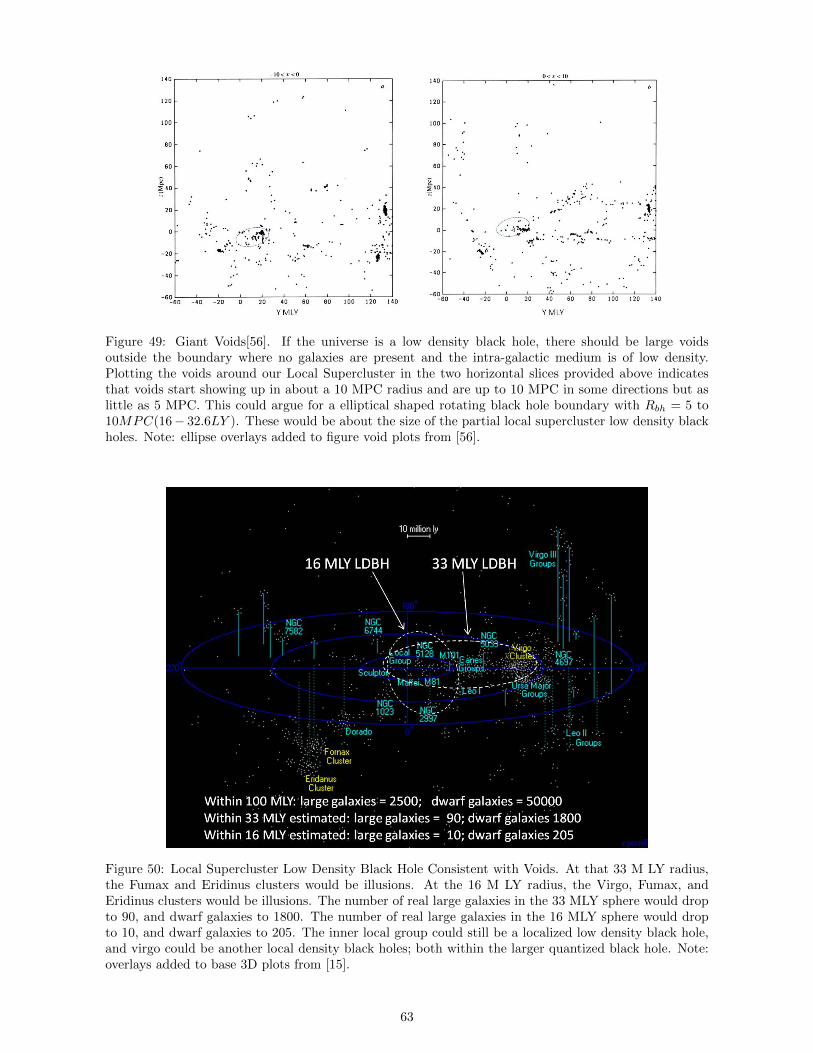
Figure 49: Giant Voids[56]. If the universe is a low density black hole, there should be large voidsoutside the boundary where no galaxies are present and the intra-galactic medium is of low density.Plotting the voids around our Local Supercluster in the two horizontal slices provided above indicatesthat voids start showing up in about a 10 MPC radius and are up to 10 MPC in some directions but aslittle as 5 MPC. This could argue for a elliptical shaped rotating black hole boundary with Rbh = 5 to10MPC(16− 32.6LY ). These would be about the size of the partial local supercluster low density blackholes. Note: ellipse overlays added to figure void plots from [56].

Figure 50: Local Supercluster Low Density Black Hole Consistent with Voids. At that 33 M LY radius,the Fumax and Eridinus clusters would be illusions. At the 16 M LY radius, the Virgo, Fumax, andEridinus clusters would be illusions. The number of real large galaxies in the 33 MLY sphere would dropto 90, and dwarf galaxies to 1800. The number of real large galaxies in the 16 MLY sphere would dropto 10, and dwarf galaxies to 205. The inner local group could still be a localized low density black hole,and virgo could be another local density black holes; both within the larger quantized black hole. Note:overlays added to base 3D plots from [15].

63

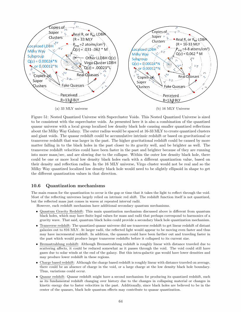
(a) 33 MLY universe (b) 16 MLY Universe

Figure 51: Nested Quantized Universe with Supercluster Voids. This Nested Quantized Universe is sizedto be consistent with the supercluster voids. As presented here it is also a combination of the quantizedquasar universe with a local group localized low density black hole causing smaller quantized reflectionsabout the Milky Way Galaxy. The outer radius would be spaced at 16-33 MLY to create quantized clustersand giant voids. The quasar redshift could be accumulative intrinsic redshift or based on gravitational ortransverse redshift that was larger in the past. The higher gravitational redshift could be caused by morematter falling in to the black holes in the past closer to its gravity well, and be brighter as well. Thetransverse redshift velocities could have been faster in the past and brighter because of they are runninginto more mass/sec, and are slowing due to the collapse. Within the outer low density black hole, therecould be one or more local low density black holes each with a different quantization value, based ontheir density and reflection radius. In the 16 MLY universe, Virgo cluster would not be real and so theMilky Way quantized localized low density black hole would need to be slightly ellipsoid in shape to getthe different quantization values in that direction.

10.6 Quantization mechanisms

The main reason for the quantization to occur is the gap or time that it takes the light to reflect through the void.Most of the reflecting universes largely relied on intrinsic red shift. The redshift function itself is not quantized,but the reflected mass just comes in waves at repeated interval radii.

However, each redshift mechanism have additional secondary quantum mechanisms.

• Quantum Gravity Redshift: This main quantization mechanism discussed above is different from quantumblack holes, which may have finite legal values for mass and radii that perhaps correspond to harmonics of agravity wave. That said, quantum black holes could provide a secondary black hole quantization mechanism.

• Transverse redshift: The quantized quasar universe did use transverse redshift to get linear redshift of distantgalaxies out to 816 MLY. At larger radii, the reflected light would appear to be moving even faster and thusmay have incremental redshift. In addition, the quasars could have been farther out and traveling faster inthe past which would produce larger transverse redshifts before it collapsed to its current size.

• Bremsstrahlung redshift: Although Bremsstrahlung redshift is roughly linear with distance traveled due toscattering affects, it could be reduced somewhat as it passes through the void. The void could still havegases due to solar winds at the end of the galaxy. But this intra-galactic gas would have lower densities andmay produce lower redshift in these regions.

• Charge based redshift: Although the charge based redshift is roughly linear with distance traveled on average,there could be an absence of charge in the void, or a large charge at the low density black hole boundary.Thus, variations could occur.

• Quasar redshift: Quasar redshift might have a second mechanism for producing its quantized redshift, suchas its fundamental redshift changing over history due to the changes in collapsing material or changes inkinetic energy due to faster velocities in the past. Additionally, since black holes are believed to be in thecenter of the quasars, black hole quantum effects may contribute to quasar quantization.

64

Again, Hawking and other have tried to reproduce these quantized red shifts, but convinced themselves that theywere not real or could be explained by other effects.

That said, as stated earlier, realize that the reflecting universes put forth in this paper do not require quantizedredshift, but if quantized redshift is observed, the low density black hole reflection mechanism could be its source.If quantized redshift are not observed, the more continuous reflections could be easily explained by the light beingreflected more continuously. That is, light does not only go straight out and in, but can easily travel in largeelliptical orbits of arbitrary lengths. The low density black holes are also not like stellar black holes with a singlestar in the center, but consist of many stars and galaxies at various depths. The light from the lower depth wouldstart to turn or be bent backwards starting at a much lower level. Thus, crisp redshift quantization values maynot be observed, but may only show up in statistical averages. Also, our measurement accuracies may not begood enough (yet) to tell.

11 Conclusion

This paper demonstrated the following related to low density black holes (LDBHs):

1. LDBHs could form at arbitrary average densities. (Rs = .0013401√Pavg

LY, Rbh = .0018952√Pavg

LY for Pavg in kg/m3).

2. LDBHs could form with a 13.8 BLY radius if the universe is at its critical density of about 5 to 10 hydrogenatoms per cubic meter.

3. LDBHs could form with a 63MLY radius if the existing galactic densities are extended with a densityequivalent to 1 hydrogen atom per 2 cubic cm.

4. LDBHs could form with 20, 6.3, or 2 MLY radius if dark matter is present or heavy dense inner or outerregion averaging between 1 atom/cm3 to 1 atom/mm3.

5. One could be living in a low density black hole and not know it.

(a) G forces and tidal forces are imperceptible

(b) Centripetal forces could keep the black hole from collapsing.

6. We are not in an expanding universe: 1) if at critical density, would have encountered a finite black holethat would have stopped expansion when half the size, 2) if larger than the critical density, would haveencountered a finite black hole (with additional mass) that would have stopped expansion when half thesize, 3) if less than the critical density, would have encountered a black hole when the universe was smallerand denser.

7. The Big Bang probably did not happen.

8. The Hubble Doppler redshift interpretation is not valid and the 13.8 BLY creation date is no longer valid.

9. LDBHs can use spin’s centripetal accelleration and/or charge to keep from collapsing.

10. LDBHs with density functions that fall off slower than 1/R2 can keep from collapsing with the appropriatespeed curve.

11. We can be in a finite low density black hole that is rotating or collapsing.

12. The Hubble redshift can no longer come from expansion, but now needs to come from transverse relativisticredshifts, gravitational redshifts, or one of the other space based intrinsic redshift mechanisms.

13. An infinite universe is possible, but will collapse into a disjoint low density black holes and escape the Olber’sparadox.

14. A non-reflecting universe could match the current expanding universes in size (e.g. 13.8 BLY) and mass,but formed inside a rotating Schwarzschild or finite low density black hole.

15. Reflecting universes could be much smaller and may be at 600, 66, 20, 6, or 1.5 M Light Years Radii. (Thiswould only require densities up to 1 hydrogen atom per cubic mm). In these cases, the entire universe couldonly be as little as 1.5 M Light Years.

16. Andromeda and Triangulum galaxies are probably real and not just reflections of the Milky Way galaxy.

17. Quantized redshift may warrant a second look as LDBHs provide a new potential source via reflections.

18. If we are within a localized black hole, additional real external galaxies could exist and be seen from ourblack hole.

19. The only non-black hole universe would be a collapsing universe below critical mass. But it could stillcontain localized black holes at the higher densities in the middle, would appear like a black hole, and willeventually collapse into a black hole.

20. Thus, we are probably in a black hole, or will be eventually.

If the research from this paper does lead to a paradigm shift, this will be an exciting time to be a cosmologist, witheverything a new. However, most of what we know would not really change. However, I think a little humilityshould be in order for a decade or two, especially if one can’t even trust what their eyes and telescopes are seeing.

65

12 Future investigations

Future directions are to:

• Vet the above theory with the scientific community and seek supporting or non-supporting evidence.

• Redo calculations using relativistic equations and KERR-NEWMANN rotating black hole equations [1, 4].

• Re-analyze galaxy and quasar redshift data for quantized redshift

• Continue mass distribution analysis using 3D data for all galaxies in the local cluster.

• Investigate reflecting potential within the Milky Way galaxy.

Acknowledgements

Although I am an amateur cosmologist, I did take a few graduate classes as ASU to help me form a foundationin order to just begin to approach this problem. I wanted to explore this idea on my own before getting theprofessionals involved. I trust now they know the reason for my silly and sometimes unreasonable questions.

Specifically, I would like to thank Astronomy Professor Aannestad who put up with me in several classes andPhysics professor Nicole Herbots-Culbertson for teaching me relativity theory. You gave me the tools to pursuethis theory. Without your knowledge, this would just be a nagging question on my “To Do” list that never gotdone. And then, I would have learned nothing. Thank you for all your help.

I would also like to recognize the Hubble Space Telescope, the Chandra Observatory, the Digital Sky Sur-vey, NASA, Wikipedia, Google Search, Google Scholar, arXiv, and the other internet publishing services whoseinformation was indispensible for this endeavor. I would also be remiss if I did not mention Newton, Einstein,Hawking, Hubble, Schwarzschild, Reissner, Nordstrom, Kerr, and Newman.

I would also like to thank my daughter Angie for helping me formalize my disproof of the Big Bang Theory(Theorem 1), checking my derivations and converting my many equations into Latex, and making my mathematicalnotations consistent. She also formatted all my references, and managed my references and figures numbersthroughout the document.

I would also like to thank any reader that made it this far. This was not an easy read, nor a simple subject.The only thing worse than taking twenty five years to write a paper, is to do so and not have anyone willing toread it. You just saved me from this most undesirable fate. I hope that you learned as much from this paper as Idid writing it.

66

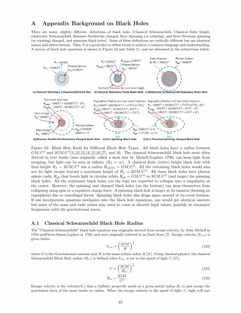
A Appendix Background on Black Holes

There are many, slightly different, definitions of black holes (Classical Schwarzschild, Classical finite height,relativistic Schwarzschild, Reissner-Nordstrom charged, Kerr Spinning (or rotating), and Kerr-Newman spinning(or rotating) charged, and quantum black holes). Some of these definitions are radically different but use identicalnames and abbreviations. Thus, it is a good idea to define terms to achieve a common language and understanding.A survey of black hole equations is shown in Figure 52 and Table 11, and are discussed in the subsections below.

Figure 52: Black Hole Radii for Different Black Hole Types. All black holes have a radius betweenGM/C2 and 2GM/C2[1],[2],[3],[4],[5],[6],[7], and [8]. The classical Schwarzschild black hole most oftenderived in text books (was originally called a dark star by Michell/Laplace 1796) can keep light fromescaping, but light can be seen at infinity (Rf = ∞). A classical finite (twice) height black hole withfinal height Rf = 2GM/C2 has a radius Rc2xbh = GM/C2. All the remaining black holes would alsonot let light escape beyond a maximum height of Rf = 2GM/C2. All these black holes have photonsphere radii, Rph that bends light in circular orbits Rph = GM/C2 to 3GM/C2 (and larger) for spinningblack holes. All the stationary black holes (on the top) are expected to collapse into a singularity atthe center. However, the spinning and charged black holes (on the bottom) can keep themselves fromcollapsing using spin or a rupulsive charge force. A spinning black hole is larger at its equator (forming anergosphere) due to centrifugal forces. Spinning black holes also drags space around at its event horizon.If one incorporates quantum mechanics into the black hole equations, one would get identical answersbut some of the mass and radii values may need to come in discrete legal values, possibly at resonancefrequencies with the gravitational waves.

A.1 Classical Schwarzschild Black Hole Radius

The ”Classical Schwarzschild” black hole equation was originally derived from escape velocity, by John Michell in1784 andPierre-Simon Laplace in 1796, and were originally referred to as Dark Stars [7]. Escape velocity (Vesc) isgiven below:

Vesc =

(2GM

R

) 12

(123)

where G is the Gravitational constant and M is the mass within radius R [31]. Using classical physics, the classicalSchwarzschild Black Hole radius (Rcs) is defined when Vesc is set to the speed of light C [57],

C =

(2GM

Rcs

) 12

(124)

Rcs =2GM

C2. (125)

Escape velocity is the velocity(Vi) that a ballistic projectile needs at a given initial radius Ri to just escape thegravitation force of the mass inside its radius. When the escape velocity is the speed of light, C, light will just

67

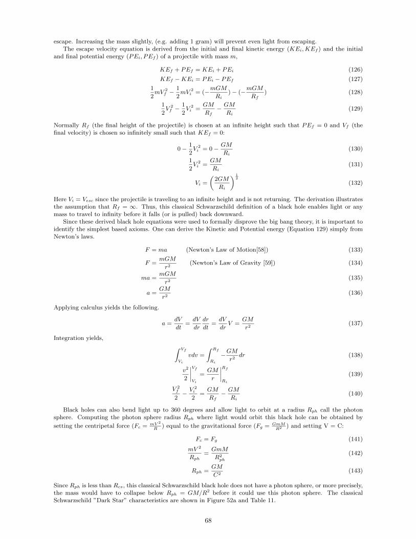
escape. Increasing the mass slightly, (e.g. adding 1 gram) will prevent even light from escaping.The escape velocity equation is derived from the initial and final kinetic energy (KEi,KEf ) and the initial

and final potential energy (PEi, PEf ) of a projectile with mass m,

KEf + PEf = KEi + PEi (126)

KEf −KEi = PEi − PEf (127)

1

2mV 2

f −1

2mV 2

i = (−mGMRi

)− (−mGMRf

) (128)

1

2V 2f −

1

2V 2i =

GM

Rf− GM

Ri(129)

Normally Rf (the final height of the projectile) is chosen at an infinite height such that PEf = 0 and Vf (thefinal velocity) is chosen so infinitely small such that KEf = 0:

0− 1

2V 2i = 0− GM

Ri(130)

1

2V 2i =

GM

Ri(131)

Vi =

(2GM

Ri

) 12

(132)

Here Vi = Vesc since the projectile is traveling to an infinite height and is not returning. The derivation illustratesthe assumption that Rf = ∞. Thus, this classical Schwarzschild definition of a black hole enables light or anymass to travel to infinity before it falls (or is pulled) back downward.

Since these derived black hole equations were used to formally disprove the big bang theory, it is important toidentify the simplest based axioms. One can derive the Kinetic and Potential energy (Equation 129) simply fromNewton’s laws.

F = ma (Newton’s Law of Motion[58]) (133)

F =mGM

r2(Newton’s Law of Gravity [59]) (134)

ma =mGM

r2(135)

a =GM

r2(136)

Applying calculus yields the following.

a =dV

dt=dV

dr

dr

dt=dV

drV =

GM

r2(137)

Integration yields, ∫ Vf

Vi

vdv =

∫ Rf

Ri

−GMr2

dr (138)

v2

2

∣∣∣∣Vf

Vi

=GM

r

∣∣∣∣Rf

Ri

(139)

V 2f

2− V 2

i

2=GM

Rf− GM

Ri(140)

Black holes can also bend light up to 360 degrees and allow light to orbit at a radius Rph call the photonsphere. Computing the photon sphere radius Rph where light would orbit this black hole can be obtained by

setting the centripetal force (Fc = mV 2

R) equal to the gravitational force (Fg = GmM

R2 ) and setting V = C:

Fc = Fg (141)

mV 2

Rph=GmM

R2ph

(142)

Rph =GM

C2(143)

Since Rph is less than Rcs, this classical Schwarzschild black hole does not have a photon sphere, or more precisely,the mass would have to collapse below Rph = GM/R2 before it could use this photon sphere. The classicalSchwarzschild ”Dark Star” characteristics are shown in Figure 52a and Table 11.

68

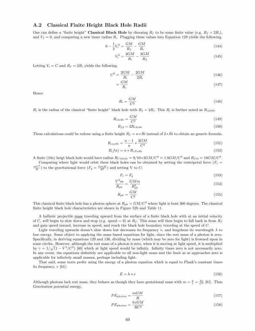
A.2 Classical Finite Height Black Hole Radii

One can define a “finite height” Classical Black Hole by choosing Rf to be some finite value (e.g. Rf = 2Ri),and Vf = 0, and computing a new inner radius Ri. Plugging these values into Equation 129 yields the following.

0− 1

2V 2i =

GM

Rf− GM

Ri(144)

V 2i =

2GM

Ri− 2GM

Rf(145)

Letting Vi = C and Rf = 2Ri yields the following.

C2 =2GM

Ri− 2GM

2Ri(146)

=GM

Ri(147)

Hence

Ri =GM

C2(148)

Ri is the radius of the classical “finite height” black hole with Rf = 2Ri. This Ri is further noted as Rc2xbh.

Rc2xbh =GM

C2(149)

Rf2 = 2Rc2xbh (150)

These calculations could be redone using a finite height Rf = n∗Ri instead of 2∗Ri to obtain an generic formula.

Rcnxbh =n− 1

n∗ 2GM

C2(151)

R(fn) = n ∗RcNxbh (152)

A finite (10x) heigt black hole would have radius RC10xbh = 9/10∗2GM/C2 = 1.8GM/C2 and Rf10 = 18GM/C2.Computing where light would orbit these black holes can be obtained by setting the centripetal force (Fc =

mV 2

R) to the gravitational force (Fg = GmM

R2 ) and setting V to C:

Fc = Fg (153)

V 2m

Rph=GMm

R2ph

(154)

Rph =GM

C2(155)

This classical finite black hole has a photon sphere at Rph = GM/C2 where light is bent 360 degrees. The classicalfinite height black hole characteristics are shown in Figure 52b and Table 11.

A ballistic projectile mass traveling upward from the surface of a finite black hole with at an initial velocityof C, will begin to slow down and stop (e.g. speed = 0) at Rf . This mass will then begin to fall back in from Rfand gain speed inward, increase in speed, and reach the black hole boundary traveling at the speed of C.

Light traveling upwards doesn’t slow down but decreases its frequency v, and lengthens its wavelength λ tolose energy. Some object to applying the mass based equations for light, since the rest mass of a photon is zero.Specifically, in deriving equations 129 and 136, dividing by mass (which may be zero for light) is frowned upon insome circles. However, although the rest mass of a photon is zero, when it is moving at light speed, it is multipliedby γ = 1/

√(1 − V 2/C2) [60] which at light speed would be infinity. Infinity times zero is not necessarily zero.

In any event, the equations definitely are applicable to all non-light mass and the limit as m approaches zero isapplicable for infinitely small masses, perhaps including light.

That said, some texts prefer using the energy of a photon equation which is equal to Plank’s constant timesits frequency, v [61]:

E = h ∗ v (156)

Although photons lack rest mass, they behave as though they have gratational mass with m = pv

= hvC2 [61]. Thus

Gravitation potential energy,

PEphoton =mGM

R(157)

PEphoton =hvGM

RC2(158)

69

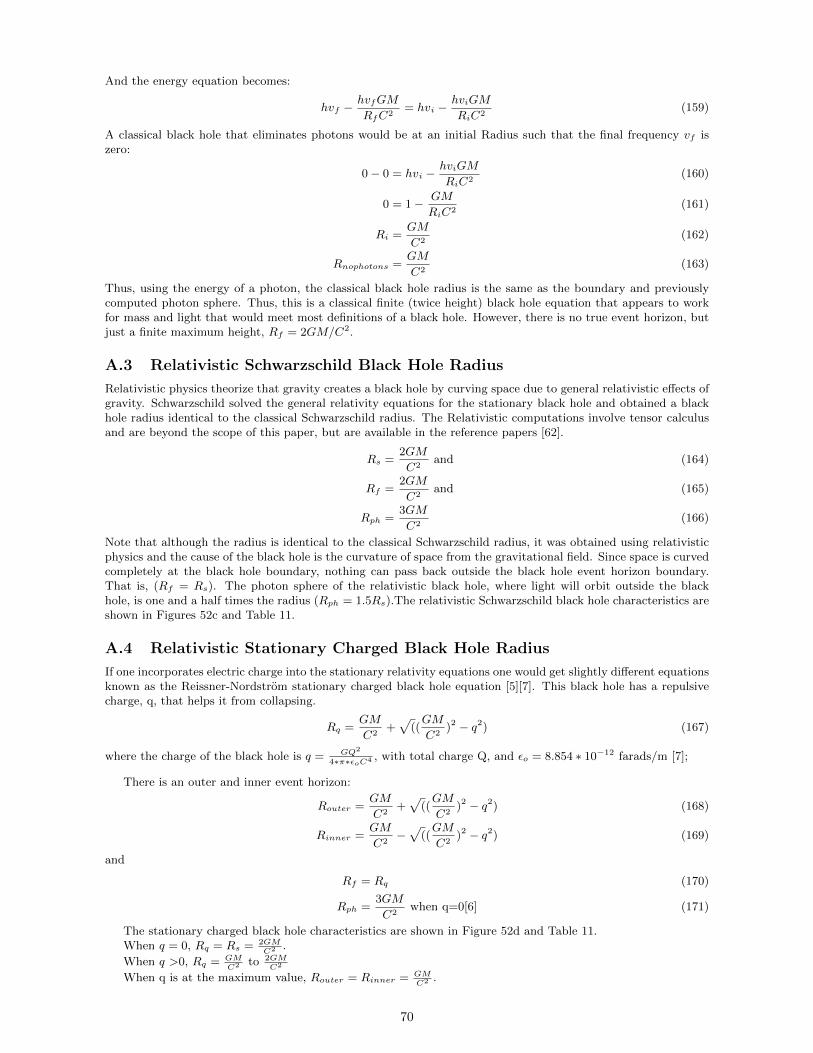
And the energy equation becomes:

hvf −hvfGM

RfC2= hvi −

hviGM

RiC2(159)

A classical black hole that eliminates photons would be at an initial Radius such that the final frequency vf iszero:

0− 0 = hvi −hviGM

RiC2(160)

0 = 1− GM

RiC2(161)

Ri =GM

C2(162)

Rnophotons =GM

C2(163)

Thus, using the energy of a photon, the classical black hole radius is the same as the boundary and previouslycomputed photon sphere. Thus, this is a classical finite (twice height) black hole equation that appears to workfor mass and light that would meet most definitions of a black hole. However, there is no true event horizon, butjust a finite maximum height, Rf = 2GM/C2.

A.3 Relativistic Schwarzschild Black Hole Radius

Relativistic physics theorize that gravity creates a black hole by curving space due to general relativistic effects ofgravity. Schwarzschild solved the general relativity equations for the stationary black hole and obtained a blackhole radius identical to the classical Schwarzschild radius. The Relativistic computations involve tensor calculusand are beyond the scope of this paper, but are available in the reference papers [62].

Rs =2GM

C2and (164)

Rf =2GM

C2and (165)

Rph =3GM

C2(166)

Note that although the radius is identical to the classical Schwarzschild radius, it was obtained using relativisticphysics and the cause of the black hole is the curvature of space from the gravitational field. Since space is curvedcompletely at the black hole boundary, nothing can pass back outside the black hole event horizon boundary.That is, (Rf = Rs). The photon sphere of the relativistic black hole, where light will orbit outside the blackhole, is one and a half times the radius (Rph = 1.5Rs).The relativistic Schwarzschild black hole characteristics areshown in Figures 52c and Table 11.

A.4 Relativistic Stationary Charged Black Hole Radius

If one incorporates electric charge into the stationary relativity equations one would get slightly different equationsknown as the Reissner-Nordstrom stationary charged black hole equation [5][7]. This black hole has a repulsivecharge, q, that helps it from collapsing.

Rq =GM

C2+√

((GM

C2)2 − q2) (167)

where the charge of the black hole is q = GQ2

4∗π∗εoC4 , with total charge Q, and εo = 8.854 ∗ 10−12 farads/m [7];

There is an outer and inner event horizon:

Router =GM

C2+√

((GM

C2)2 − q2) (168)

Rinner =GM

C2−√

((GM

C2)2 − q2) (169)

and

Rf = Rq (170)

Rph =3GM

C2when q=0[6] (171)

The stationary charged black hole characteristics are shown in Figure 52d and Table 11.When q = 0, Rq = Rs = 2GM

C2 .

When q >0, Rq = GMC2 to 2GM

C2

When q is at the maximum value, Router = Rinner = GMC2 .

70

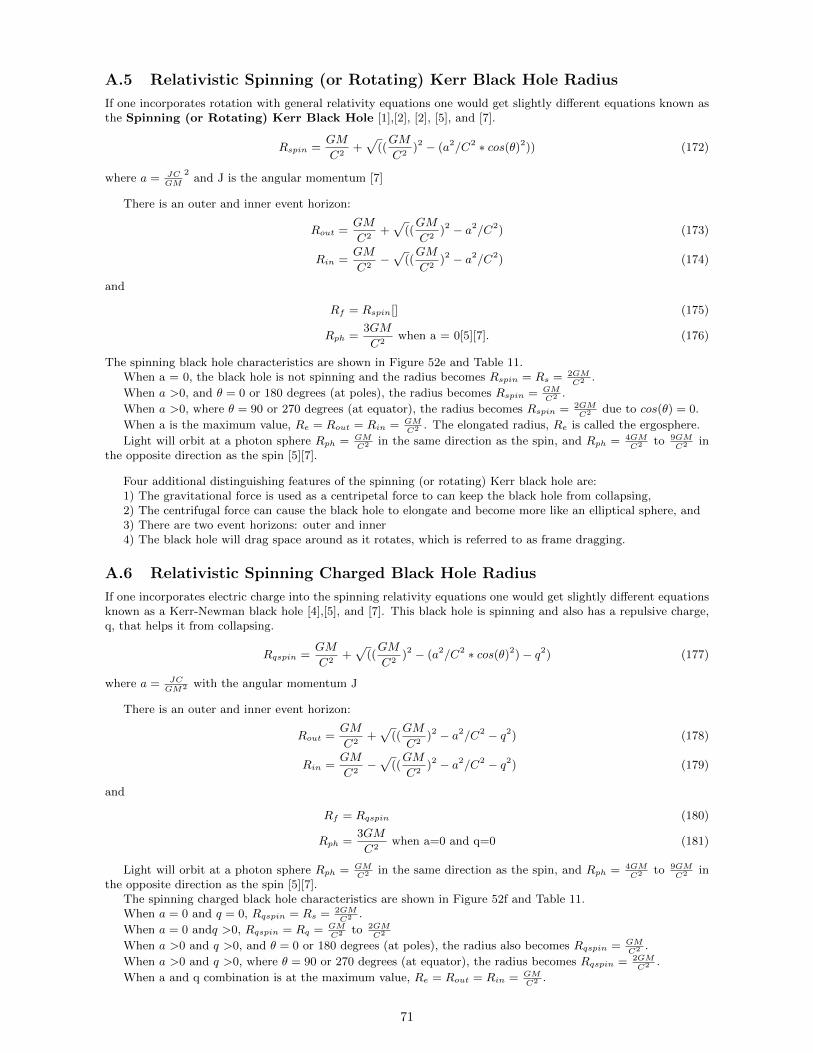
A.5 Relativistic Spinning (or Rotating) Kerr Black Hole Radius

If one incorporates rotation with general relativity equations one would get slightly different equations known asthe Spinning (or Rotating) Kerr Black Hole [1],[2], [2], [5], and [7].

Rspin =GM

C2+√

((GM

C2)2 − (a2/C2 ∗ cos(θ)2)) (172)

where a = JCGM

2and J is the angular momentum [7]

There is an outer and inner event horizon:

Rout =GM

C2+√

((GM

C2)2 − a2/C2) (173)

Rin =GM

C2−√

((GM

C2)2 − a2/C2) (174)

and

Rf = Rspin[] (175)

Rph =3GM

C2when a = 0[5][7]. (176)

The spinning black hole characteristics are shown in Figure 52e and Table 11.When a = 0, the black hole is not spinning and the radius becomes Rspin = Rs = 2GM

C2 .

When a >0, and θ = 0 or 180 degrees (at poles), the radius becomes Rspin = GMC2 .

When a >0, where θ = 90 or 270 degrees (at equator), the radius becomes Rspin = 2GMC2 due to cos(θ) = 0.

When a is the maximum value, Re = Rout = Rin = GMC2 . The elongated radius, Re is called the ergosphere.

Light will orbit at a photon sphere Rph = GMC2 in the same direction as the spin, and Rph = 4GM

C2 to 9GMC2 in

the opposite direction as the spin [5][7].

Four additional distinguishing features of the spinning (or rotating) Kerr black hole are:1) The gravitational force is used as a centripetal force to can keep the black hole from collapsing,2) The centrifugal force can cause the black hole to elongate and become more like an elliptical sphere, and3) There are two event horizons: outer and inner4) The black hole will drag space around as it rotates, which is referred to as frame dragging.

A.6 Relativistic Spinning Charged Black Hole Radius

If one incorporates electric charge into the spinning relativity equations one would get slightly different equationsknown as a Kerr-Newman black hole [4],[5], and [7]. This black hole is spinning and also has a repulsive charge,q, that helps it from collapsing.

Rqspin =GM

C2+√

((GM

C2)2 − (a2/C2 ∗ cos(θ)2)− q2) (177)

where a = JCGM2 with the angular momentum J

There is an outer and inner event horizon:

Rout =GM

C2+√

((GM

C2)2 − a2/C2 − q2) (178)

Rin =GM

C2−√

((GM

C2)2 − a2/C2 − q2) (179)

and

Rf = Rqspin (180)

Rph =3GM

C2when a=0 and q=0 (181)

Light will orbit at a photon sphere Rph = GMC2 in the same direction as the spin, and Rph = 4GM

C2 to 9GMC2 in

the opposite direction as the spin [5][7].The spinning charged black hole characteristics are shown in Figure 52f and Table 11.When a = 0 and q = 0, Rqspin = Rs = 2GM

C2 .

When a = 0 andq >0, Rqspin = Rq = GMC2 to 2GM

C2

When a >0 and q >0, and θ = 0 or 180 degrees (at poles), the radius also becomes Rqspin = GMC2 .

When a >0 and q >0, where θ = 90 or 270 degrees (at equator), the radius becomes Rqspin = 2GMC2 .

When a and q combination is at the maximum value, Re = Rout = Rin = GMC2 .

71

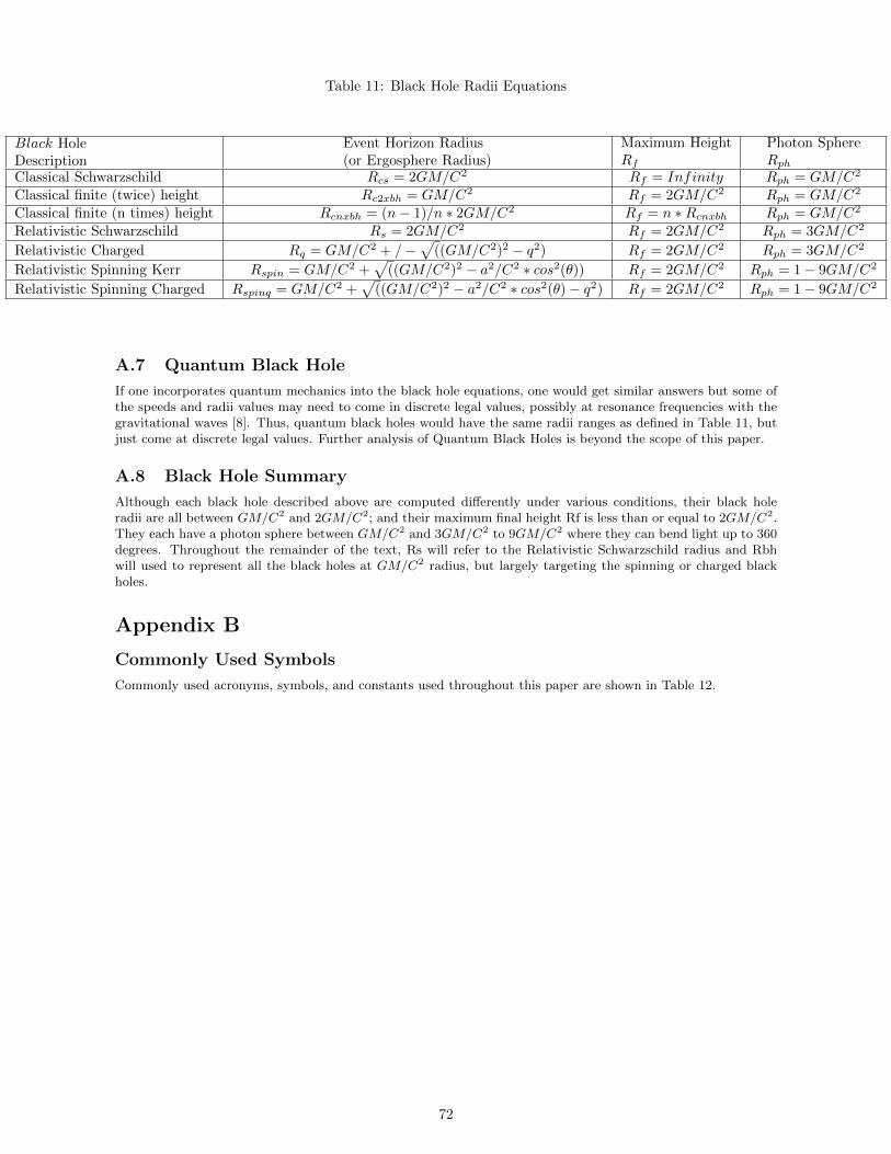
Table 11: Black Hole Radii Equations

Black HoleDescription

Event Horizon Radius(or Ergosphere Radius)

Maximum HeightRf

Photon SphereRph

Classical Schwarzschild Rcs = 2GM/C2 Rf = Infinity Rph = GM/C2

Classical finite (twice) height Rc2xbh = GM/C2 Rf = 2GM/C2 Rph = GM/C2

Classical finite (n times) height Rcnxbh = (n− 1)/n ∗ 2GM/C2 Rf = n ∗Rcnxbh Rph = GM/C2

Relativistic Schwarzschild Rs = 2GM/C2 Rf = 2GM/C2 Rph = 3GM/C2

Relativistic Charged Rq = GM/C2 + /−√

((GM/C2)2 − q2) Rf = 2GM/C2 Rph = 3GM/C2

Relativistic Spinning Kerr Rspin = GM/C2 +√

((GM/C2)2 − a2/C2 ∗ cos2(θ)) Rf = 2GM/C2 Rph = 1− 9GM/C2

Relativistic Spinning Charged Rspinq = GM/C2 +√

((GM/C2)2 − a2/C2 ∗ cos2(θ)− q2) Rf = 2GM/C2 Rph = 1− 9GM/C2

A.7 Quantum Black Hole

If one incorporates quantum mechanics into the black hole equations, one would get similar answers but some ofthe speeds and radii values may need to come in discrete legal values, possibly at resonance frequencies with thegravitational waves [8]. Thus, quantum black holes would have the same radii ranges as defined in Table 11, butjust come at discrete legal values. Further analysis of Quantum Black Holes is beyond the scope of this paper.

A.8 Black Hole Summary

Although each black hole described above are computed differently under various conditions, their black holeradii are all between GM/C2 and 2GM/C2; and their maximum final height Rf is less than or equal to 2GM/C2.They each have a photon sphere between GM/C2 and 3GM/C2 to 9GM/C2 where they can bend light up to 360degrees. Throughout the remainder of the text, Rs will refer to the Relativistic Schwarzschild radius and Rbhwill used to represent all the black holes at GM/C2 radius, but largely targeting the spinning or charged blackholes.

Appendix B

Commonly Used Symbols

Commonly used acronyms, symbols, and constants used throughout this paper are shown in Table 12.

72

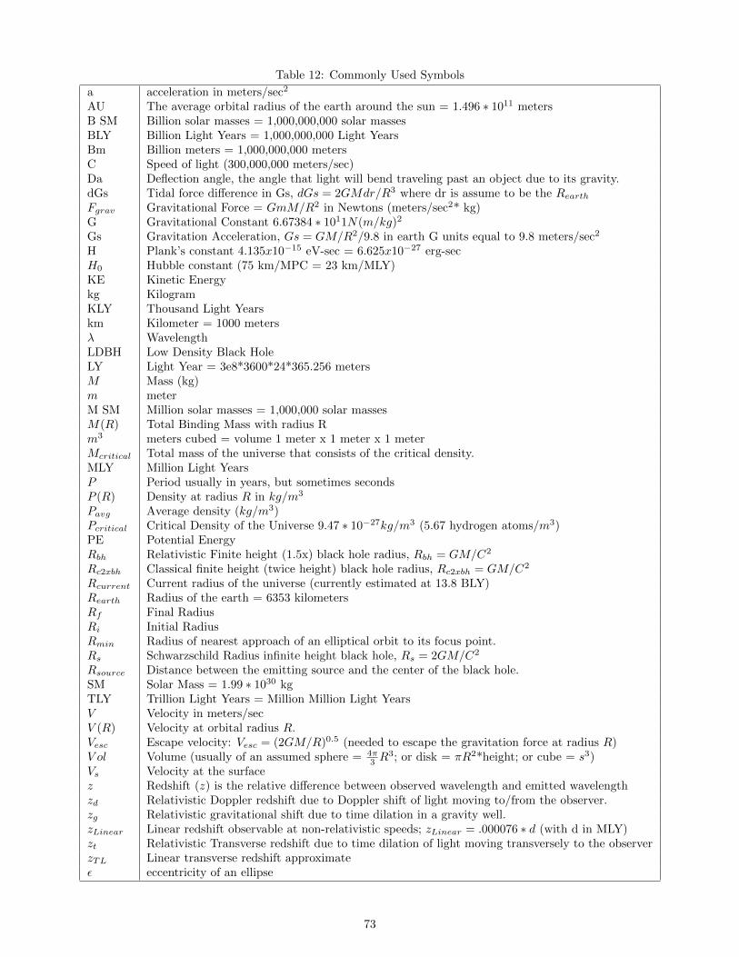
Table 12: Commonly Used Symbols

a acceleration in meters/sec2

AU The average orbital radius of the earth around the sun = 1.496 ∗ 1011 metersB SM Billion solar masses = 1,000,000,000 solar massesBLY Billion Light Years = 1,000,000,000 Light YearsBm Billion meters = 1,000,000,000 metersC Speed of light (300,000,000 meters/sec)Da Deflection angle, the angle that light will bend traveling past an object due to its gravity.dGs Tidal force difference in Gs, dGs = 2GMdr/R3 where dr is assume to be the RearthFgrav Gravitational Force = GmM/R2 in Newtons (meters/sec2* kg)G Gravitational Constant 6.67384 ∗ 1011N(m/kg)2

Gs Gravitation Acceleration, Gs = GM/R2/9.8 in earth G units equal to 9.8 meters/sec2

H Plank’s constant 4.135x10−15 eV-sec = 6.625x10−27 erg-secH0 Hubble constant (75 km/MPC = 23 km/MLY)KE Kinetic Energykg KilogramKLY Thousand Light Yearskm Kilometer = 1000 metersλ WavelengthLDBH Low Density Black HoleLY Light Year = 3e8*3600*24*365.256 metersM Mass (kg)m meterM SM Million solar masses = 1,000,000 solar massesM(R) Total Binding Mass with radius Rm3 meters cubed = volume 1 meter x 1 meter x 1 meterMcritical Total mass of the universe that consists of the critical density.MLY Million Light YearsP Period usually in years, but sometimes secondsP (R) Density at radius R in kg/m3

Pavg Average density (kg/m3)Pcritical Critical Density of the Universe 9.47 ∗ 10−27kg/m3 (5.67 hydrogen atoms/m3)PE Potential EnergyRbh Relativistic Finite height (1.5x) black hole radius, Rbh = GM/C2

Rc2xbh Classical finite height (twice height) black hole radius, Rc2xbh = GM/C2

Rcurrent Current radius of the universe (currently estimated at 13.8 BLY)Rearth Radius of the earth = 6353 kilometersRf Final RadiusRi Initial RadiusRmin Radius of nearest approach of an elliptical orbit to its focus point.Rs Schwarzschild Radius infinite height black hole, Rs = 2GM/C2

Rsource Distance between the emitting source and the center of the black hole.SM Solar Mass = 1.99 ∗ 1030 kgTLY Trillion Light Years = Million Million Light YearsV Velocity in meters/secV (R) Velocity at orbital radius R.Vesc Escape velocity: Vesc = (2GM/R)0.5 (needed to escape the gravitation force at radius R)V ol Volume (usually of an assumed sphere = 4π

3 R3; or disk = πR2*height; or cube = s3)

Vs Velocity at the surfacez Redshift (z) is the relative difference between observed wavelength and emitted wavelengthzd Relativistic Doppler redshift due to Doppler shift of light moving to/from the observer.zg Relativistic gravitational shift due to time dilation in a gravity well.zLinear Linear redshift observable at non-relativistic speeds; zLinear = .000076 ∗ d (with d in MLY)zt Relativistic Transverse redshift due to time dilation of light moving transversely to the observerzTL Linear transverse redshift approximateε eccentricity of an ellipse

73

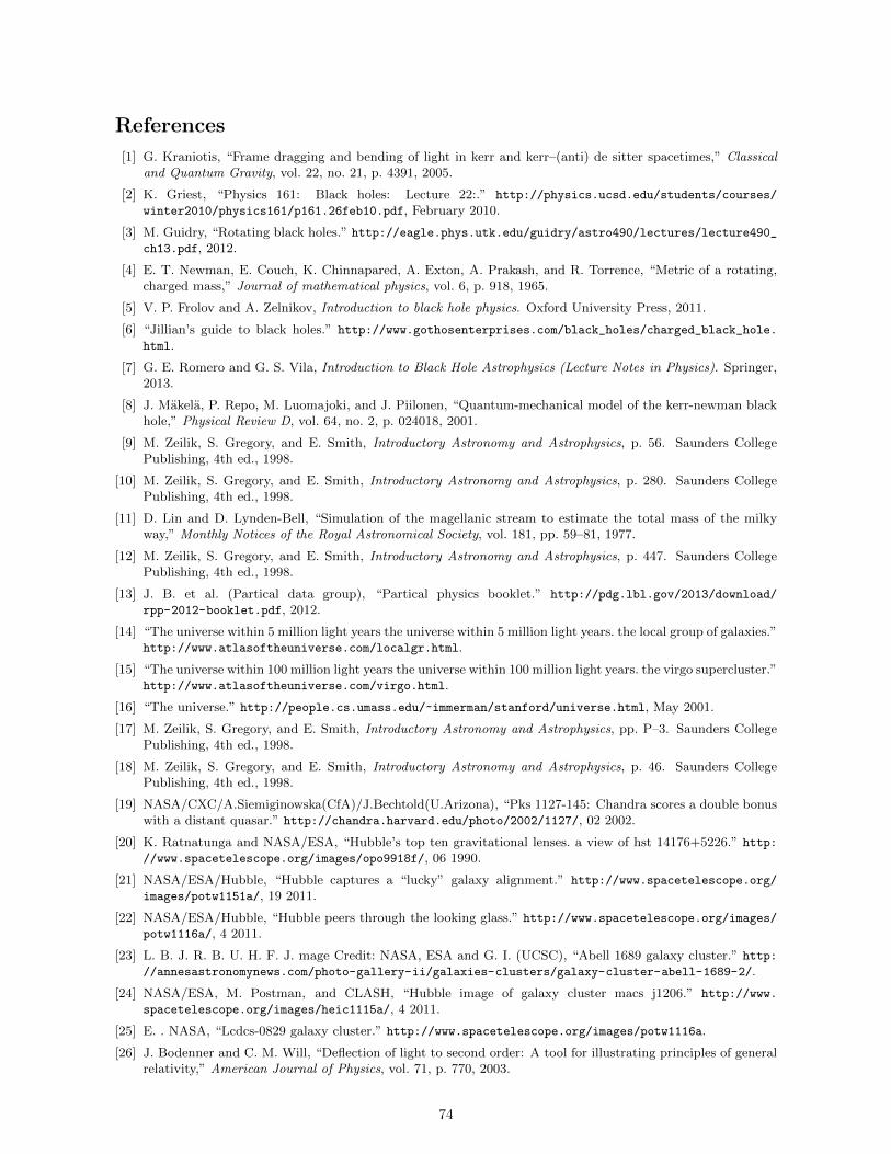
References

[1] G. Kraniotis, “Frame dragging and bending of light in kerr and kerr–(anti) de sitter spacetimes,” Classicaland Quantum Gravity, vol. 22, no. 21, p. 4391, 2005.

[2] K. Griest, “Physics 161: Black holes: Lecture 22:.” http://physics.ucsd.edu/students/courses/

winter2010/physics161/p161.26feb10.pdf, February 2010.

[3] M. Guidry, “Rotating black holes.” http://eagle.phys.utk.edu/guidry/astro490/lectures/lecture490_

ch13.pdf, 2012.

[4] E. T. Newman, E. Couch, K. Chinnapared, A. Exton, A. Prakash, and R. Torrence, “Metric of a rotating,charged mass,” Journal of mathematical physics, vol. 6, p. 918, 1965.

[5] V. P. Frolov and A. Zelnikov, Introduction to black hole physics. Oxford University Press, 2011.

[6] “Jillian’s guide to black holes.” http://www.gothosenterprises.com/black_holes/charged_black_hole.

html.

[7] G. E. Romero and G. S. Vila, Introduction to Black Hole Astrophysics (Lecture Notes in Physics). Springer,2013.

[8] J. Makela, P. Repo, M. Luomajoki, and J. Piilonen, “Quantum-mechanical model of the kerr-newman blackhole,” Physical Review D, vol. 64, no. 2, p. 024018, 2001.

[9] M. Zeilik, S. Gregory, and E. Smith, Introductory Astronomy and Astrophysics, p. 56. Saunders CollegePublishing, 4th ed., 1998.

[10] M. Zeilik, S. Gregory, and E. Smith, Introductory Astronomy and Astrophysics, p. 280. Saunders CollegePublishing, 4th ed., 1998.

[11] D. Lin and D. Lynden-Bell, “Simulation of the magellanic stream to estimate the total mass of the milkyway,” Monthly Notices of the Royal Astronomical Society, vol. 181, pp. 59–81, 1977.

[12] M. Zeilik, S. Gregory, and E. Smith, Introductory Astronomy and Astrophysics, p. 447. Saunders CollegePublishing, 4th ed., 1998.

[13] J. B. et al. (Partical data group), “Partical physics booklet.” http://pdg.lbl.gov/2013/download/

rpp-2012-booklet.pdf, 2012.

[14] “The universe within 5 million light years the universe within 5 million light years. the local group of galaxies.”http://www.atlasoftheuniverse.com/localgr.html.

[15] “The universe within 100 million light years the universe within 100 million light years. the virgo supercluster.”http://www.atlasoftheuniverse.com/virgo.html.

[16] “The universe.” http://people.cs.umass.edu/~immerman/stanford/universe.html, May 2001.

[17] M. Zeilik, S. Gregory, and E. Smith, Introductory Astronomy and Astrophysics, pp. P–3. Saunders CollegePublishing, 4th ed., 1998.

[18] M. Zeilik, S. Gregory, and E. Smith, Introductory Astronomy and Astrophysics, p. 46. Saunders CollegePublishing, 4th ed., 1998.

[19] NASA/CXC/A.Siemiginowska(CfA)/J.Bechtold(U.Arizona), “Pks 1127-145: Chandra scores a double bonuswith a distant quasar.” http://chandra.harvard.edu/photo/2002/1127/, 02 2002.

[20] K. Ratnatunga and NASA/ESA, “Hubble’s top ten gravitational lenses. a view of hst 14176+5226.” http:

//www.spacetelescope.org/images/opo9918f/, 06 1990.

[21] NASA/ESA/Hubble, “Hubble captures a “lucky” galaxy alignment.” http://www.spacetelescope.org/

images/potw1151a/, 19 2011.

[22] NASA/ESA/Hubble, “Hubble peers through the looking glass.” http://www.spacetelescope.org/images/

potw1116a/, 4 2011.

[23] L. B. J. R. B. U. H. F. J. mage Credit: NASA, ESA and G. I. (UCSC), “Abell 1689 galaxy cluster.” http:

//annesastronomynews.com/photo-gallery-ii/galaxies-clusters/galaxy-cluster-abell-1689-2/.

[24] NASA/ESA, M. Postman, and CLASH, “Hubble image of galaxy cluster macs j1206.” http://www.

spacetelescope.org/images/heic1115a/, 4 2011.

[25] E. . NASA, “Lcdcs-0829 galaxy cluster.” http://www.spacetelescope.org/images/potw1116a.

[26] J. Bodenner and C. M. Will, “Deflection of light to second order: A tool for illustrating principles of generalrelativity,” American Journal of Physics, vol. 71, p. 770, 2003.

74

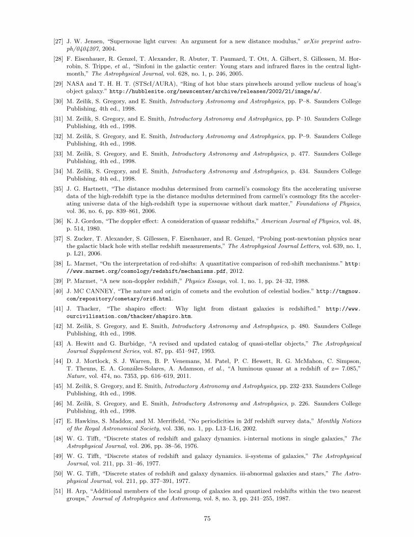
[27] J. W. Jensen, “Supernovae light curves: An argument for a new distance modulus,” arXiv preprint astro-ph/0404207, 2004.

[28] F. Eisenhauer, R. Genzel, T. Alexander, R. Abuter, T. Paumard, T. Ott, A. Gilbert, S. Gillessen, M. Hor-robin, S. Trippe, et al., “Sinfoni in the galactic center: Young stars and infrared flares in the central light-month,” The Astrophysical Journal, vol. 628, no. 1, p. 246, 2005.

[29] NASA and T. H. H. T. (STScI/AURA), “Ring of hot blue stars pinwheels around yellow nucleus of hoag’sobject galaxy.” http://hubblesite.org/newscenter/archive/releases/2002/21/image/a/.

[30] M. Zeilik, S. Gregory, and E. Smith, Introductory Astronomy and Astrophysics, pp. P–8. Saunders CollegePublishing, 4th ed., 1998.

[31] M. Zeilik, S. Gregory, and E. Smith, Introductory Astronomy and Astrophysics, pp. P–10. Saunders CollegePublishing, 4th ed., 1998.

[32] M. Zeilik, S. Gregory, and E. Smith, Introductory Astronomy and Astrophysics, pp. P–9. Saunders CollegePublishing, 4th ed., 1998.

[33] M. Zeilik, S. Gregory, and E. Smith, Introductory Astronomy and Astrophysics, p. 477. Saunders CollegePublishing, 4th ed., 1998.

[34] M. Zeilik, S. Gregory, and E. Smith, Introductory Astronomy and Astrophysics, p. 434. Saunders CollegePublishing, 4th ed., 1998.

[35] J. G. Hartnett, “The distance modulus determined from carmeli’s cosmology fits the accelerating universedata of the high-redshift type ia the distance modulus determined from carmeli’s cosmology fits the acceler-ating universe data of the high-redshift type ia supernovae without dark matter,” Foundations of Physics,vol. 36, no. 6, pp. 839–861, 2006.

[36] K. J. Gordon, “The doppler effect: A consideration of quasar redshifts,” American Journal of Physics, vol. 48,p. 514, 1980.

[37] S. Zucker, T. Alexander, S. Gillessen, F. Eisenhauer, and R. Genzel, “Probing post-newtonian physics nearthe galactic black hole with stellar redshift measurements,” The Astrophysical Journal Letters, vol. 639, no. 1,p. L21, 2006.

[38] L. Marmet, “On the interpretation of red-shifts: A quantitative comparison of red-shift mechanisms.” http:

//www.marmet.org/cosmology/redshift/mechanisms.pdf, 2012.

[39] P. Marmet, “A new non-doppler redshift,” Physics Essays, vol. 1, no. 1, pp. 24–32, 1988.

[40] J. MC CANNEY, “The nature and origin of comets and the evolution of celestial bodies.” http://tmgnow.

com/repository/cometary/ori6.html.

[41] J. Thacker, “The shapiro effect: Why light from distant galaxies is redshifted.” http://www.

ourcivilisation.com/thacker/shapiro.htm.

[42] M. Zeilik, S. Gregory, and E. Smith, Introductory Astronomy and Astrophysics, p. 480. Saunders CollegePublishing, 4th ed., 1998.

[43] A. Hewitt and G. Burbidge, “A revised and updated catalog of quasi-stellar objects,” The AstrophysicalJournal Supplement Series, vol. 87, pp. 451–947, 1993.

[44] D. J. Mortlock, S. J. Warren, B. P. Venemans, M. Patel, P. C. Hewett, R. G. McMahon, C. Simpson,T. Theuns, E. A. Gonzales-Solares, A. Adamson, et al., “A luminous quasar at a redshift of z= 7.085,”Nature, vol. 474, no. 7353, pp. 616–619, 2011.

[45] M. Zeilik, S. Gregory, and E. Smith, Introductory Astronomy and Astrophysics, pp. 232–233. Saunders CollegePublishing, 4th ed., 1998.

[46] M. Zeilik, S. Gregory, and E. Smith, Introductory Astronomy and Astrophysics, p. 226. Saunders CollegePublishing, 4th ed., 1998.

[47] E. Hawkins, S. Maddox, and M. Merrifield, “No periodicities in 2df redshift survey data,” Monthly Noticesof the Royal Astronomical Society, vol. 336, no. 1, pp. L13–L16, 2002.

[48] W. G. Tifft, “Discrete states of redshift and galaxy dynamics. i-internal motions in single galaxies,” TheAstrophysical Journal, vol. 206, pp. 38–56, 1976.

[49] W. G. Tifft, “Discrete states of redshift and galaxy dynamics. ii-systems of galaxies,” The AstrophysicalJournal, vol. 211, pp. 31–46, 1977.

[50] W. G. Tifft, “Discrete states of redshift and galaxy dynamics. iii-abnormal galaxies and stars,” The Astro-physical Journal, vol. 211, pp. 377–391, 1977.

[51] H. Arp, “Additional members of the local group of galaxies and quantized redshifts within the two nearestgroups,” Journal of Astrophysics and Astronomy, vol. 8, no. 3, pp. 241–255, 1987.

75

[52] W. Napier and B. Guthrie, “Quantized redshifts: a status report,” Journal of Astrophysics and Astronomy,vol. 18, no. 4, pp. 455–463, 1997.

[53] W. Tifft, “Global redshift periodicities and periodicity structure,” The Astrophysical Journal, vol. 468, p. 491,1996.

[54] W. G. Tifft, “Global redshift periodicities and variability,” The Astrophysical Journal, vol. 485, no. 2, p. 465,1997.

[55] M. Bell, “Discrete intrinsic redshifts from quasars to normal galaxies,” Arxiv preprint astro-ph/0211091,2002.

[56] Y. B. Zeldovich, J. Einasto, and S. Shandarin, “Giant voids in the universe,” Nature, vol. 300, no. 5891,pp. 407–413, 1982.

[57] M. Zeilik, S. Gregory, and E. Smith, Introductory Astronomy and Astrophysics, p. 346. Saunders CollegePublishing, 4th ed., 1998.

[58] M. Zeilik, S. Gregory, and E. Smith, Introductory Astronomy and Astrophysics, p. 11. Saunders CollegePublishing, 4th ed., 1998.

[59] M. Zeilik, S. Gregory, and E. Smith, Introductory Astronomy and Astrophysics, p. 13. Saunders CollegePublishing, 4th ed., 1998.

[60] H. D. Young and R. A. Freedman, Sears and Zemansky’s university physics, vol. 1, p. 1290. Pearson education,2006.

[61] A. Beiser, Concepts of modern physics, pp. 83–86, 326–327. McGraw-Hill New York, 5 ed., 1995.

[62] J. A. Rybczyk, “Relativistic event horizon for black holes.” http://www.mrelativity.net/

RelEventHorizon/Relativistic%20Event%20Horizon%20for%20Black%20Holes.htm, 2009.

76