BER performance of MC-DS-CDMA systems in the presence … · BER Performance of MC-DS-CDMA Systems in the Presence of Timing Jitter . A thesis presented in partial fulfillment of

Copyright is owned by the Author of the thesis. Permission is given for a copy to be downloaded by an individual for the purpose of research and private study only. The thesis may not be reproduced elsewhere without the permission of the Author.

BER Performance of MC-DS-CDMA Systems in the Presence

of Timing Jitter

A thesis presented in partial fulfillment of the requirements for the

Degree of

Master of Engineering

in

Information and Telecommunications Engineering

at Massey University, Palmerston North,

New Zealand.

Lindong Xu

2010

Acknowledgement

I would like to express my gratitude to all those who guided and assisted me to

accomplish this thesis. First and foremost, I gratefully acknowledge the help of my

supervisor Dr. Xiang Gui. I do appreciate his patience, encouragement, and

professional instructions during my thesis writing. The completion of this thesis would

be impossible without his guidance, supervision and assistance. Many thanks to my

best friend Rui Li who always shares his research experience with me.

I also would like to take this opportunity to express my heartfelt gratitude to my

beloved parents who have always been helping me out of difficulties and supporting

and caring for me all of my life.

BER Performance of MC-DS-CDMA Systems in the Presence of

Timing Jitter

Abstract

Multi-carrier direct-sequence code division multiple access (MC-DS-CDMA)

technique, which is a combination of orthogonal frequency-division multiplexing

(OFDM) and code division multiple accesses (CDMA), has been considered as an

important technique for the future generation wireless systems due to its bandwidth

efficiency, frequency diversity, and immunity to channel dispersion. OFDM has

already been employed in many areas, such as digital audio and video broadcasting,

wireless local/metropolitan area networks, and asynchronous digital subscriber lines

(ADSL). Leveraging the multiple access capability of CDMA, the MC-DS-CDMA

technique is an important enhancement to OFDM.

Nevertheless, a major disadvantage of the MC-DS-CDMA systems is their high

sensitivity to timing errors between transmitter and receiver due to the use of a large

number of carriers and the superposition of signals of multiple users. In this thesis,

we study the bit error rate (BER) performance of MC-DS-CDMA system under the

effects of timing jitter in additive white Gaussian noise (AWGN) channel and

multi-path Rayleigh fading channel, respectively. In particular, we have derived

the analytical BER expressions for the MC-DS-CDMA signals in presence of white

or colored timing jitters and verified the results via computer simulations.

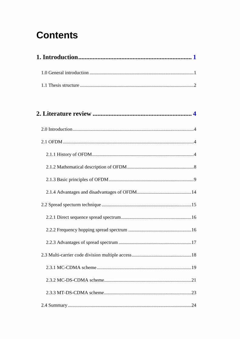
Contents

1. Introduction ....................................................................... 1

1.0 General introduction ...................................................................................... 1 1.1 Thesis structure .............................................................................................. 2

2. Literature review .............................................................. 4 2.0 Introduction .................................................................................................... 4 2.1 OFDM ............................................................................................................ 4

2.1.1 History of OFDM .................................................................................... 4 2.1.2 Mathematical description of OFDM ....................................................... 8 2.1.3 Basic principles of OFDM ...................................................................... 9 2.1.4 Advantages and disadvantages of OFDM............................................. 14

2.2 Spread specturm technique .......................................................................... 15

2.2.1 Direct sequence spread spectrum .......................................................... 16 2.2.2 Frequency hopping spread spectrum .................................................... 16

2.2.3 Advantages of spread spectrum ............................................................ 17

2.3 Multi-carrier code division multiple access ................................................. 18

2.3.1 MC-CDMA scheme .............................................................................. 19

2.3.2 MC-DS-CDMA scheme........................................................................ 21

2.3.3 MT-DS-CDMA scheme ........................................................................ 23

2.4 Summary ...................................................................................................... 24

3. Implementation of the MC-DS-CDMA system ............ 26 3.0 Introduction .................................................................................................. 26 3.1 Transmitter ................................................................................................... 27 3.2 Dual OVSF spreading codes ........................................................................ 29 3.3 Channel simulation ...................................................................................... 35 3.4 Receiver ....................................................................................................... 38 3.5 Simulation results and conclusions .............................................................. 39

4. BER performance analysis on the effect of timing jitter 42 4.0 Introduction .................................................................................................. 42 4.1 Problem formulation .................................................................................... 42 4.2 ICI due to timing jitter ................................................................................. 44

4.2.1 ICI due to white timing jitter ................................................................ 47

4.2.2 ICI due to colored timing jitter ............................................................. 53

5. BER performance test methods ..................................... 59 5.0 Introduction .................................................................................................. 59 5.1 Testing method in AWGN channel.............................................................. 59

5.2 Testing methods in multi-path Rayleigh fading channel ............................. 59

6. Results and discussion .................................................... 61 6.1 BER performance on the effect of timing jitter in AWGN channel ............ 61

6.2 BER performance on the effect of timing jitters in multi-path Rayleigh fading channel ......................................................................................................... 70

7. Conclusion ....................................................................... 74

References ............................................................................ 75

Appendix: Complete Matlab codes ................................... 81

A1 OVSF code ............................................................................................... 81

A2 Simulation code of the MC-DS-CDMA system in AWGN channel ..... 83

A3 Simulation code of the MC-DS-CDMA system in multi-path Rayleigh fading channel ........................................................................................ 87

List of Figures

Figure 2.1 Comparison of the bandwidth utilization for FDM and OFDM................6 Figure 2.2 (A) Spectrum of an OFDM sub-carrier (B) Spectrum of an OFDM

signal. ........................................................................................................6 Figure 2.3 Block diagram of an FFT-based OFDM system .....................................10 Figure 2.4 Example of the guard interval .................................................................12 Figure 2.5 Time and frequency representation of OFDM using guard interval. ......13 Figure 2.6 Direct sequence speard spectrum (DSSS) block diagram .......................16 Figure 2.7 Frequency hopping speard spectrum (FHSS) block diagram ..................17 Figure 2.8 The transmitter diagram of MC-CDMA scheme ....................................19 Figure 2.9 The receiver diagram of MC-CDMA scheme .........................................20 Figure 2.10 The transmitter diagram of MC-DS-CDMA scheme. ...........................21 Figure 2.11 The receiver diagram of MC-DS-CDMA scheme.................................22 Figure 2.12 The transmitter diagram of MT-DS-CDMA scheme .......................... 23 Figure 2.13 The reveiver diagram of MT-DS-CDMA scheme. ................................24 Figure 3.1 Block diagram of four-user MC-DS-CDMA system ..............................27 Figure 3.2 Block diagram of MC-DS-CDMA transmitter for a single-user. ............29 Figure 3.3 Multi-path demonstration. .......................................................................36 Figure 3.4 Block diagram of MC-DS-CDMA channel model ..................................38 Figure 3.5 Block diagram of MC-DS-CDMA receiver ............................................39 Figure 3.6 BER curves of SUI Channels ..................................................................40

List of Tables Table 3.1 Comparison of peak correlation values: length-4 HOVSF and dual OVSF

...................................................................................................................35 Table 3.2 Comparison of peak correlation values: length-8 HOVSF and dual OVSF

...................................................................................................................35 Table 3.3 Parameters of SUI-1 ..................................................................................37 Table 3.4 Parameters of SUI-2 ..................................................................................37 Table 3.5 Parameters of SUI-3 ..................................................................................37 Table 3.6 Parameters of SUI-4 ..................................................................................37 Table 3.7 Parameters of SUI-5 ..................................................................................37 Table 3.8 Parameters of SUI-6 ..................................................................................38 Table 3.9 BER of SUI-1 Channel .............................................................................40 Table 3.10 BER of SUI-2 Channel ...........................................................................40 Table 3.11 BER of SUI-3 Channel ...........................................................................41 Table 3.12 BER of SUI-4 Channel ...........................................................................41 Table 3.13 BER of SUI-5 Channel ...........................................................................41 Table 3.14 BER of SUI-6 Channel ...........................................................................41

List of Abbreviations

MC-DS-CDMA: multi-carrier direct-sequence code division multiple access

OFDM: orthogonal frequency-division multiplexing

CDMA: code division multiple access

ADSL: asynchronous digital subscriber lines

BER: bit error rate

AWGN: additive white Gaussian noise

MCM: multi-carrier modulation

SP: serial-to-parallel

SNR: signal-to-noise ratio

OVSF: orthogonal variable spreading factor

FFT: Fast Fourier Transform

DMT: discrete multi-tone

FDM: frequency division multiplexing

FDMA: frequency division multiplexing access

VLSI: very-large-scale integration

QAM: quadrature amplitude modulation

HDSL: high-bit-rate digital subscriber lines

VHDSL: very high-speed digital subscriber lines

DAB: digital audio broadcasting

FM: frequency modulation

IFFT: inverse Fast Fourier Transform

ISI: inter-symbol interference

D/A: digital to analog

LPF: low-pass filter

RF: radio frequency

ICI: inter-carrier interference

SS: spread spectrum

DSSS: direct sequence spread spectrum

FHSS: frequency hopping spread spectrum

PN: pseudo-noise

FFHSS: fast frequency-hopping spread-spectrum

SFHSS: slow frequency-hopping spread-spectrum

MC-CDMA: multi-carrier orthogonal frequency-division multiplexing

MT-DS-CDMA: multi-tone direct-sequence code division multiple access

FEC: forward error control

4G: fourth-generation

HOVSF: Hadamard orthogonal variable spreading factor

JOVSF: Jacket orthogonal variable spreading factor

SUI: Stanford University Interim

1

1. Introduction

1.0 General introduction

Multi-carrier modulation (MCM) that is known as orthogonal frequency-division

multiplexing (OFDM) has drawn considerable attention in high speed mobile

communications due to its bandwidth efficiency, frequency diversity, and immunity to

channel dispersion during the last decade. Currently, MCM is being used in digital

audio and video broadcasting, wireless local/metropolitan area networks, and

asynchronous digital subscriber lines (ADSL) [1]. With recent advances in modulation

and multiple access techniques, MCM becomes more and more popular.

Today, the enormous increase in demand for high-speed data transmission by many

wireless multi-media services pushes the development of advanced modulation and

multiple access techniques that can provide reliable and high data rate transmission with

high bandwidth efficiency and strong immunity to multi-path distortion.

Recently, different combinations of OFDM and code division multiple accesses (CDMA)

have been investigated and presented by various researchers. One of these combinations

is the multi-carrier direct-sequence code division multiple access (MC-DS-CDMA)

technique, which has been considered as an important technique for the

fourth-generation wireless systems [2]. In the MC-DS-CDMA systems, the transmitter

transmits the serial-to-parallel (SP) converted data stream using a given spreading

sequence in the time domain, so that the resultant spectrum of each sub-carrier can

remain orthogonal and keep the minimum required frequency separation.

Nevertheless, a major disadvantage of multi-carrier direct-sequence code division

multiple access (MC-DS-CDMA) systems is their high sensitivity to timing errors

between transmitter and receiver due to the use of a large number of carriers. The

influence of timing errors on multi-carrier systems has been reported in [45, 46] for

OFDM and in [39] for MC-DS-CDMA. In [45] and [46], it was shown that the OFDM

2

system suffers severely from a clock frequency offset between the transmitter and the

receiver. In [39], the effect of timing jitter on MC-DS-CDMA was studied in terms of

signal-to-noise ratio (SNR) degradation. While SNR is indicative of the performance

of digital communication systems, the bit error rate (BER) is the direct performance

measure. In this thesis, we extend the results of [39] and study the BER performance

of MC-DS-CDMA system under the effects of timing jitter in additive white Gaussian

noise (AWGN) channel and multi-path Rayleigh fading channel, respectively. In

particular, we have derived the analytical BER expressions for the MC-DS-CDMA

signals in presence of white or colored timing jitters and verified the results via

computer simulations.

1.1 Thesis structure

This thesis is organized as seven chapters and one appendix.

Chapter 2 gives a literature review related to our research including orthogonal

frequency division multiplexing technique, spreading spectrum technique, and

multi-carrier code division multiple access technique.

Chapter 3 presents an MC-DS-CDMA system simulated in AWGN channel and

multi-path Rayleigh fading channel using Simulink in Matlab. The simulation of

transmitter, channel and receiver are described in this chapter. The orthogonal variable

spreading factor (OVSF) codes used as spreading codes in our research are also

presented.

Chapter 4 describes the analysis of BER performance of MC-DS-CDMA system due to

timing jitter in AWGN channel and multi-path Rayleigh fading channel, respectively. The

analytical BER expressions for MC-DS-CDMA in presence of white and colored timing

jitters are formulated and discussed.

Chapter 5 introduces the algorithm we used to test the BER performance of

MC-DS-CDMA system.

3

Chapter 6 shows the test results of the system. A discussion is also included.

Chapter 7 contains the conclusion of this thesis.

The appendix contains the simulation algorithm codes.

4

2. Literature review

2.0 Introduction

Our research is on MC-DS-CDMA and the simulation is based on Simulink and

programming in Matlab. Related topics are OFDM, spread spectrum, and combinations of

MCM and CDMA. We will present a literature review of these topics in the following

sections.

2.1 OFDM

MCM is a method to data transmission that divides data stream into several sub-streams and

deliver each of these sub-streams to modulate carrier signals. With recent advances in

efficient implementation of Fast Fourier Transform (FFT), the MCM concept is becoming

widely adopted in practical applications. It can be found in IEEE standards 802.11a,

802.15.3 and 802.16a, as well as standards for digital broadcasting of television and radio [3].

MCM has been referred to by different names such as discrete multi-tone (DMT) modulation

in wire line communication and OFDM in wireless communication. We will use OFDM in

this thesis.

We next present the history, mathematical description and basic principles of OFDM.

2.1.1 History of OFDM

Frequency division multiplexing (FDM) is a technology that transmits multiple signals

simultaneously over a single transmission path. In frequency division multiplexing access

(FDMA) each user is typically allocated a single channel that is used to transmit all the

user information, each signal travels within its own unique frequency range (carrier),

which is modulated by the data [4].

5

OFDM is a transmission technique based on the idea of FDM. In OFDM, the transmitter

transmits a single data stream over a number of lower rate orthogonal sub-carriers

coupled with the use of advanced modulation techniques on each component, resulting in

a signal with high resistance to interference. OFDM can be simply defined as

multi-carrier modulation where its carrier spacing is carefully selected so that each

sub-carrier is orthogonal to the other sub-carriers [5]. One main reason to use OFDM is to

increase the robustness against frequency selective fading or narrowband interference. In

a single carrier system, a single fade or interference can cause the entire link to fail, but in

a multi-carrier system, only a small percentage of the sub-carriers will be affected. Then

error correction coding can be used to correct for the few erroneous sub-carriers. The

concept of using parallel data transmission and FDM was published in the mid-1960s [6,

7]. Some early development can be traced back in the 1950s [8]. A U.S. patent was filed

and issued in January, 1970 [9].

In a classical parallel data system, the total signal frequency band is divided into

non-overlapping frequency sub-channels. Each sub-channel is modulated with a separate

symbol and then the sub-channels are frequency-multiplexed. It seems good to avoid

spectral overlap of channels and eliminate inter-channel interference. However, this leads

to inefficient use of the available spectrum. To cope with the inefficiency, the ideas

proposed from the mid-1960s were to use parallel data and FDM with overlapping

sub-channels to avoid the use of high speed equalization and to combat impulsive noise,

and multi-path distortion as well as to fully use the available bandwidth [10].

Conventional FDM multi-carrier modulation technique

6

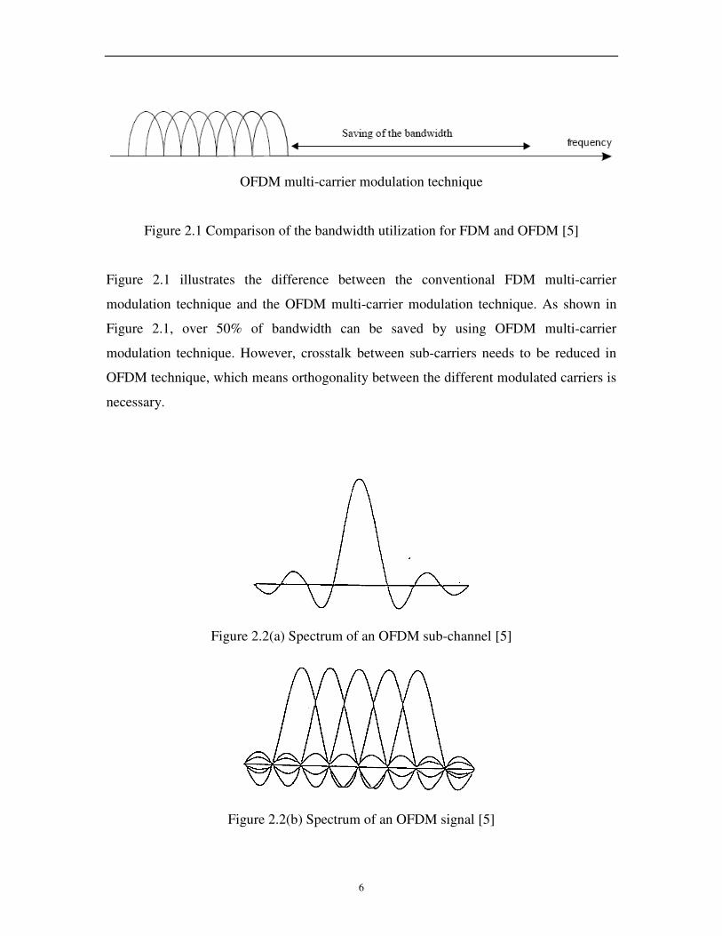
OFDM multi-carrier modulation technique

Figure 2.1 Comparison of the bandwidth utilization for FDM and OFDM [5]

Figure 2.1 illustrates the difference between the conventional FDM multi-carrier

modulation technique and the OFDM multi-carrier modulation technique. As shown in

Figure 2.1, over 50% of bandwidth can be saved by using OFDM multi-carrier

modulation technique. However, crosstalk between sub-carriers needs to be reduced in

OFDM technique, which means orthogonality between the different modulated carriers is

necessary.

Figure 2.2(a) Spectrum of an OFDM sub-channel [5]

Figure 2.2(b) Spectrum of an OFDM signal [5]

7

Much of the research focuses on the highly efficient multi-carrier transmission scheme

based on orthogonal frequency carriers. In 1971, Weinstein and Ebert applied the discrete

Fourier transform (DFT) to parallel data transmission systems as part of the modulation

and demodulation processes [11]. Figure 2.2(a) shows the spectrum of an OFDM

sub-channel and Figure 2.2 (b) presents the spectrum of the OFDM signal. From Figure

2.2, it can be seen that at the central frequency of each sub-channel, there are no cross

talks from other channels. Therefore, if we use DFT at the receiver and calculate

correlation values with the center of frequency of each sub-carrier, the transmitted data

could be recovered with no crosstalk.

Moreover, to eliminating the banks of sub-carrier oscillators and coherent demodulators

required by FDM, a completely digital implementation could be built around

special-purpose hardware performing the fast Fourier transform (FFT), which is an

efficient implementation of the DFT. Recent advances in very-large-scale integration

(VLSI) technology make high speed and large size FFT chips commercially affordable

[12]. Consequently, both transmitter and receiver are implemented using efficient FFT

techniques that reduce the number of operations from 2N in DFT down to NN log

where N is the FFT size [13].

In the 1960s, the OFDM technique was used in several high-frequency military systems

such as KINEPLEX [8], ANDEFT [14] and KATHRYN [15, 16]. For example, the

variable-rate data modem in KATHRYN was built for the high-frequency band. It used

up to 34 parallel low-rate phase-modulated channels with a spacing of 82 Hz.

In the 1980s, OFDM was studied for high-speed modems, digital mobile communications,

and high-density recording. One of the systems realized the OFDM techniques for

multiplexed quadrature amplitude modulation (QAM) using DFT [17]. Furthermore,

variable-speed modems were developed for telephone networks [19].

In the 1990s, OFDM was employed for wideband data communications over mobile

8

radio channels, high-bit-rate digital subscriber lines (HDSL, 1.6 Mbps), asymmetric

digital subscriber lines (ADSL, up to 6 Mbps), very high-speed digital subscriber lines

(VHDSL, 100 Mbps), digital audio broadcasting (DAB), and digital television and

high-definition television (HDTV) terrestrial broadcasting [10]. Casas and Leung

proposed OFDM/frequency modulation (FM) for data communication over mobile radio

channels [20]. It claimed that OFDM/FM systems could be implemented simply and

inexpensively by retrofitting existing FM radio systems. Chow et al, studied the

multi-tone modulation with DFT in transceiver design and showed that it is an excellent

method for delivering of high speed data to customers, both in terms of performance and

cost, for ADSL (1.536 Mbps), HDSL (1.6 Mbps), and VHDSL (100 Mbps) [21, 22].

2.1.2 Mathematical description of OFDM

Following the history of OFDM, we discuss the mathematical definition of the OFDM

system. This allows us to see how the signal is generated and how receiver must operate,

and it gives us a tool to understand the effects of imperfections in the transmission

channel. As presented above, OFDM transmits a large number of narrowband

sub-carriers, closely spaced in the frequency domain. In order to avoid a large number of

modulators and filters at the transmitter and complementary filters and demodulators at

the receiver, it is desirable to be able to use modern digital signal processing techniques,

such as FFT [5].

Mathematically, each modulated OFDM sub-carrier can be represented as the real part of

the following complex signal

[ ]( )( ) ( ) c cj t t

c cS t A t e

ω φ+= , (2.1)

where c

ω is the sub-carrier angular frequency; while )(tAc and ( )c

tφ represent

amplitude and phase modulation on the sub-carrier, respectively, and varies from symbol

to symbol. OFDM consists of many sub-carriers. Therefore, the complex OFDM signal

)(tSs with N sub-carriers can be written as

9

[ ]1

( )

0

1( ) ( ) n n

Nj t t

s n

n

S t A t eN

ω φ−

+

=

= ∑ , (2.2)

where 0nnω ω ω= + ∆ and ω∆ is the sub-carrier spacing in angular frequency.

The amplitude and phase modulation do not change within an OFDM symbol, hence An(t)

and φn(t) can be rewritten as An and φn, respectively, when equation 2.2 is used to

represent the waveform of a single OFDM symbol. If the symbol waveform is sampled

at a sampling frequency of T

1, where T = Ts/N and Ts is the duration of one OFDM

symbol, then the resulting signal samples are given by

[ ]0

1( )

0

1( ) n

Nj n kT

s n

n

S kT A eN

ω ω φ−

+ ∆ +

=

= ∑ , k = 0, 1, …, N-1. (2.3)

Without a loss of generality by assuming 00 =ω , equation 2.3 can be simplified as:

1( )

0

1( ) n

Nj j n kT

s n

n

S kT A e eN

φ ω−

∆

=

= ∑ , k = 0, 1, …, N-1. (2.4)

Let

1 1

2s

fNT T

ω

π

∆∆ = = = , (2.5)

equation 2.4 becomes equation 2.6, which is the general form of the Inverse DFT (IDFT).

12 /

0

1( ) n

Nj j nk N

s n

n

S kT A e eN

φ π−

=

= ∑ , k = 0, 1, …, N-1. (2.6)

Equation 2.5 is the same condition that is required for sub-carrier orthogonality. Thus, the

OFDM signal can be defined by using Fourier Transform procedures [5].

2.1.3 Basic principles of OFDM

a. Generation of sub-carriers using IDFT

Consider a data sequence 0 1 -1 ( , ,..., , )n N

d d d d d= … , where nj

n n n nd A e a jb

φ= = + .

According to the definition of the N -point IDFT, which is

10

[ ] [ ]1

(2 / )

0

1 Nj N kn

n

x k X n eN

π−

=

= ∑ , (2.7)

the data sequence d can be written as a vector 0 1 -1 ( , ,..., , ) m N

D D D D D= … after

performing DFT.

1 12(2 / )

0 0

1 1n m

N Nj f tj nm N

m n n

n n

D d e d eN N

ππ− −

= =

= =∑ ∑ , m =0, 1, … N-1, (2.8)

where /( )n s

f n NT n T= = ,m

t mT= and T is the time interval of n

d .

The real part of the vector D is

{ }1

0

1Re [ cos(2 ) sin(2 )]

N

m m n n m n n m

n

Y D a f t b f tN

π π−

=

= = −∑ , m =0, 1, … N-1. (2.9)

If the samples mY is applied to a low-pass filter at time interval T, then the obtained

signal is the continuous-time OFDM waveform.

1

0

1( ) [ cos(2 ) sin(2 )]

N

n n n n

n

y t a f t b f tN

π π−

=

= −∑ , 0s

t T≤ ≤ . (2.10)

Figure 2.3: Block diagram of an FFT-based OFDM system [10]

Figure 2.3 presents the block diagram of a typical FFT-based OFDM system. At

11

transmitter side, the original serial data is first serial-to-parallel converted and grouped

into x-bits and then mappered to complex numbers. Then the complex numbers are

modulated in the baseband using the inverse FFT (IFFT) and converted back to serial

data for transmission. In order to avoid inter-symbol interference (ISI) caused by

multi-path distortion, a guard interval is inserted between symbols. Finally, the symbols

are converted from digital to analog (D/A) and low-pass filtered (LPF) for radio

frequency (RF) up-conversion. At receiver side, the inverse process of the transmitter is

performed and one-tap equalizer is used to correct channel distortion. The

tap-coefficients of the filter are calculated according to the channel information [10].

b. Guard interval and cyclic extension

Theoretically, the orthogonality of sub-channels in OFDM can be maintained and

individual sub-channels can be completely separated by the FFT at the receiver. However,

these conditions can not be obtained in practice due to inter-symbol interference (ISI) and

inter-carrier interference (ICI) introduced by transmission channel distortion. Linear

channel distortions such as multi-path can cause each sub-channel to spread energy into

the adjacent channels and make crosstalk between different sub-carriers. Consequently,

this results in ISI and ICI.

In order to prevent multi-path components interfering from one symbol with the next

symbol, a cyclically extended guard interval, which is a periodic extension of each

OFDM symbol itself, is applied for each OFDM symbol. The total symbol duration is

td g sT T T= + , where

gT is the duration of guard interval and

sT is the duration of useful

symbol. If the guard interval is chosen longer than the channel impulse response or the

multi-path delay, the ISI and ICI could be eliminated [10]. The ratio of the guard interval

to useful symbol duration depends on different systems. Since the insertion of guard

interval will reduce data throughput, g

T is usually less than 4s

T [23].

12

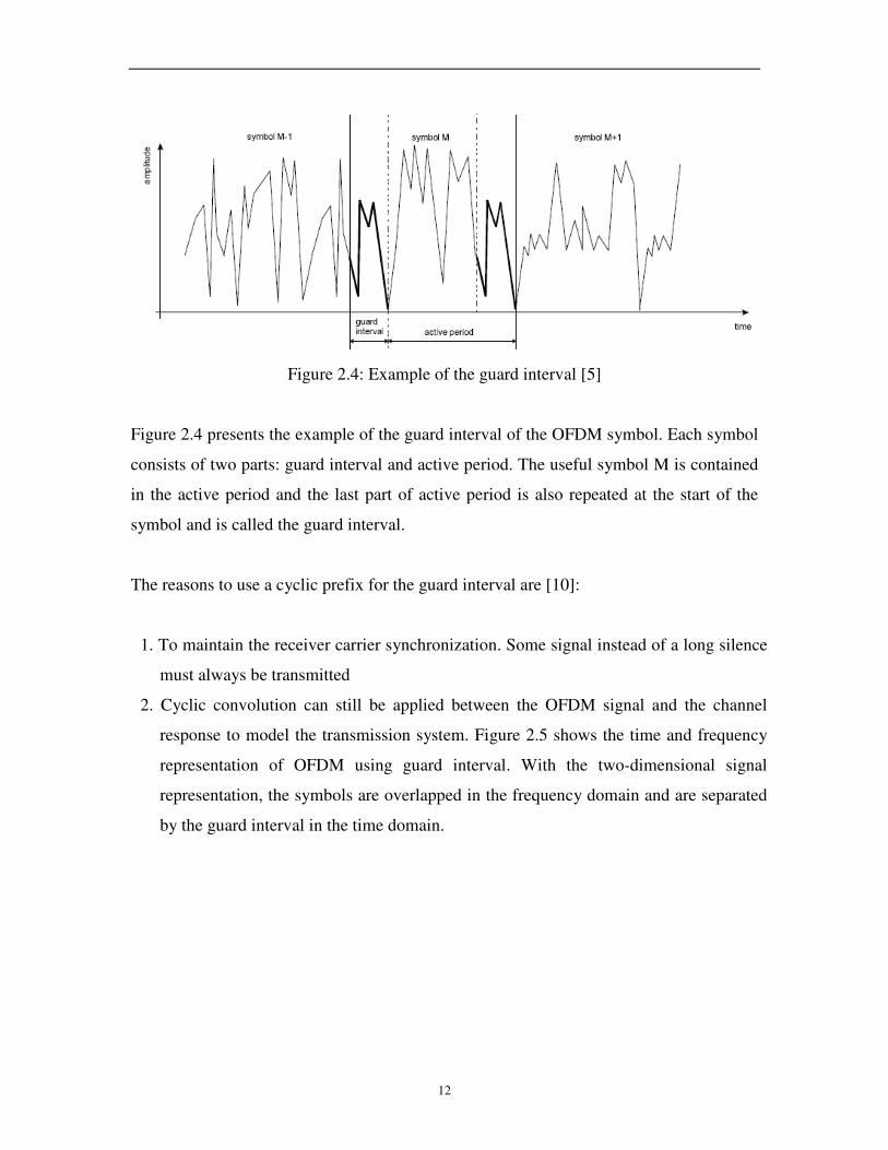
Figure 2.4: Example of the guard interval [5]

Figure 2.4 presents the example of the guard interval of the OFDM symbol. Each symbol

consists of two parts: guard interval and active period. The useful symbol M is contained

in the active period and the last part of active period is also repeated at the start of the

symbol and is called the guard interval.

The reasons to use a cyclic prefix for the guard interval are [10]:

1. To maintain the receiver carrier synchronization. Some signal instead of a long silence

must always be transmitted

2. Cyclic convolution can still be applied between the OFDM signal and the channel

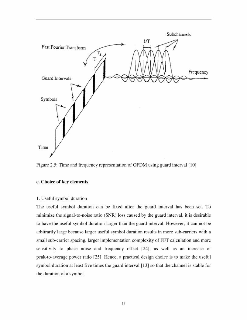
response to model the transmission system. Figure 2.5 shows the time and frequency

representation of OFDM using guard interval. With the two-dimensional signal

representation, the symbols are overlapped in the frequency domain and are separated

by the guard interval in the time domain.

13

Figure 2.5: Time and frequency representation of OFDM using guard interval [10]

c. Choice of key elements

1. Useful symbol duration

The useful symbol duration can be fixed after the guard interval has been set. To

minimize the signal-to-noise ratio (SNR) loss caused by the guard interval, it is desirable

to have the useful symbol duration larger than the guard interval. However, it can not be

arbitrarily large because larger useful symbol duration results in more sub-carriers with a

small sub-carrier spacing, larger implementation complexity of FFT calculation and more

sensitivity to phase noise and frequency offset [24], as well as an increase of

peak-to-average power ratio [25]. Hence, a practical design choice is to make the useful

symbol duration at least five times the guard interval [13] so that the channel is stable for

the duration of a symbol.

14

2. Number of sub-carriers

After the symbol duration and guard interval are fixed, the number of sub-carriers can be

determined by the required bit rate divided by the bit rate per sub-carrier. The bit rate per

sub-carrier is defined based on the modulation type, coding rate and the useful symbol

duration. What is more, the number of sub-carriers corresponds to the number of complex

points being processed in FFT. In HDTV applications, the number of sub-carriers is in

the range of several thousands so as to accommodate the data rate and guard interval

requirement [5].

3. Modulation scheme

The modulation scheme in an OFDM system can be chosen based on the requirement of

power or spectrum efficiency. The type of modulation can be specified by the complex

number n n n

d a jb= + , which is defined in the section 2.1.3a. The symbols na and n

b

can be set as ( 1, 3)± ± for 16-QAM and 1± for QPSK [5]. In general, the selection of

the modulation scheme applying to each sub-channel depends on the compromise

between the data rate requirement and transmission robustness. Furthermore, another

advantage of OFDM is that different modulation schemes can be used on different

sub-channels for layered services [5].

2.1.4 Advantages and disadvantages of OFDM

The OFDM transmission scheme has the following key advantages [13]:

1. OFDM is an efficient way to deal with multi-path. The overall signal spectrum is

divided into narrowband flat-fading sub-channels. As a result, channel equalization is

accomplished through a simple bank of complex-valued multipliers, thereby avoiding

the need for computationally demanding time domain equalizers.

2. OFDM significantly enhances the capability of interference suppression through the

use of the cyclic prefix.

3. OFDM is robust against frequency selective fading and narrowband interference,

because such interference affects only a small percentage of the sub-carriers.

15

4. OFDM has higher spectral efficiency. More than 50% of the bandwidth can be saved

compared with FDM due to overlapping sub-carriers in the frequency domain.

5. OFDM makes digital implementation simple by using DFT/IDFT operations.

6. OFDM provides an opportunity of selecting the most appropriate coding and

modulation scheme on each individual sub-carrier according to the measured channel

quality. In practice, higher order constellations are normally used on less attenuated

sub-carriers in order to increase the data throughput, while robust low-order

modulations are employed over sub-carriers characterized by low SNR values.

On the other hand, OFDM suffers from the following drawbacks compared with

single-carrier modulations:

1. OFDM is more sensitive to frequency synchronization errors and phase noise.

2. OFDM has a relatively large peak-to-average power ratio, which tends to reduce the

power efficiency of the RF amplifier.

3. OFDM has an inherent loss in spectral efficiency related to the use of the cyclic prefix.

2.2 Spread spectrum technique

The term spread spectrum (SS) has been used in a wide variety of military and

commercial communication systems. It was first described on paper by an actress and a

musician in 1941 [26] and was developed by military due to the use of wideband signals

which are difficult to detect. In recent years, SS has become increasingly popular for

commercial applications, especially in local area wireless networks.

Spread spectrum is a signal structuring technique that each signal to be transmitted

requires significantly more RF bandwidth than a conventional modulated signal would

require. In SS system, a sequential noise-like signal structure is used to spread normal

narrowband information signal over a large bandwidth in frequency domain and receiver

correlates received signals to retrieve the original information signal. That is to say, the

16

information signal is spread as wide bandwidth as possible and as close to the

background noise as possible in SS system. This makes SS communication very difficult

to find in the frequency spectrum and can not be easily tracked and more difficult to jam

[27]. There are two different types of spread spectrum techniques that have been

extensively used. These are direct sequence spread spectrum (DSSS) and frequency

hopping spread spectrum (FHSS). We will describe both techniques in the following

sections.

2.2.1 Direct sequence spread spectrum

Direct sequence is one of the most popular types of spread spectrum techniques. In this

method, a spreading signal which is a high-speed pseudo-noise (PN) code sequence

created by a pseudo-random code generator is directly multiplied with narrow-band PSK

modulated signal. Thus, desired transmission radio frequency (RF) bandwidth can be set

directly by the spreading signal.

Antenna

Modulator Chain

Power amplifier

Figure 2.6 Direct sequence speared spectrum (DSSS) block diagram

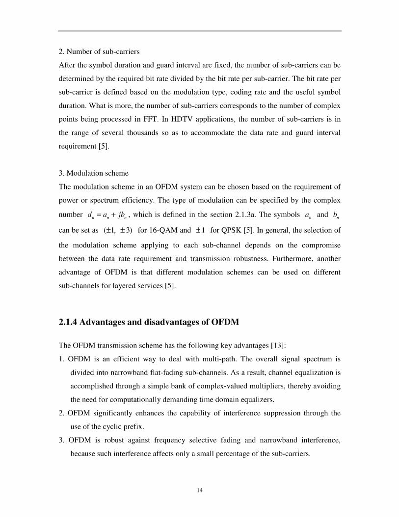
2.2.2 Frequency hopping spread spectrum

Frequency hopping is another type of spread spectrum technique which has an

PSK modulated

signal

PN code generator

RF frequency

Synthesizer

17

implementation concept similar to that of DSSS technique. In this method, spreading

occurs by hopping frequency synthesizer to one of many available frequencies over a

wide band according to a hopping table defined by the PN sequence generator. If the

hopping rate, which is chip rate, is higher than the bit rate, then it is called fast

frequency-hopping spread-spectrum (FFHSS). If the hipping rate is slower than the data

rate, there are several or many bits per frequency hop, and then it is called slow

frequency-hopping spread-spectrum (SFHSS).

Antenna

Modulator chain

Power amplifier

Figure 2.7 Frequency hopping speared spectrum (FHSS) block diagram

2.2.3 Advantages of spread spectrum technique

The spread spectrum technique has the following key advantages [28]:

1. Improved interference rejection.

2. Low-density power spectra for signal hiding.

3. High-resolution ranging.

4. Secure communications.

5. Anti-jamming capability.

6. Lower cost of implementation

7. Graceful degradation of performance as the number of simultaneous users of an RF

channel increases.

FSK modulated

signal

RF frequency

Synthesizer PN code generator

18

2.3 Multi-carrier code division multiple access

Recently, a number of CDMA systems based on the combination of CDMA schemes and

OFDM technique, which are referred to as multi-carrier CDMA systems, has received a

lot of attention in the field of wireless communications due to their effectiveness in

combating the effects of multi-path fading channels and various kinds of interference in

high speed data transmission by spreading signals over several carriers. Among these

systems, the signal can be efficiently modulated and demodulated using Fast Fourier

Transform (FFT) device without substantially increasing the transmitter and receiver’s

complexity and these systems also exhibit the attractive features of high spectral

efficiency and frequency diversity [29].

Depending on whether all the sub-carriers are activated on each transmission, multiple

access schemes based on a combination of CDMA and OFDM technique can be

classified as three types: multi-carrier CDMA (MC-CDMA), multi-carrier DS-CDMA

(MC-DS-CDMA) and multi-tone DS-CDMA (MT-DS-CDMA), which were developed

and presented by different researchers, namely, MC-CDMA by N.Yee, J-P.Linnartz and

G.Fettweis, K.Fazel and L.Papke, and A.Chouly, A.Brajal and S.Jourdan; MC-DS-CDMA

by V.DaSilva and E.S.Sousa; and MT-DS-CDMA by L.Vandendorpe [30]. The following

section will review the three types of multi-carrier CDMA schemes mentioned above.

19

2.3.1 MC-CDMA scheme

[ ]0kc ( )tf02cos π ( )tsk

Data 2232

。。

。 [ ]1kc 。 ( )tf12cos π

。。

[ ]1−pk Nc ( )tfpN 12cos −π

Figure 2.8 The transmitter diagram of MC-CDMA scheme

Figure 2.8 shows the transmitter diagram of the MC-CDMA scheme. The MC-CDMA

transmitter spreads the original serial data stream over pN , which is the number of

sub-carriers as well as the spreading gain, sub-carriers by a given spreading code of

[ ] [ ] [ ]{ },1,....1,0 −pkkk Nccc in the frequency domain. In this scheme, it does not include

serial-to-parallel data conversion and no spreading modulation is implemented on each

sub-carrier. Therefore, the data rate on each of the pN sub-carriers is the same as the

input data rate and the fading effects of multi-path channels can be mitigated by

spreading each data bit across all of the pN sub-carriers [29].

1

2

pN

1

2

∑

pN

20

( )tf02cos π ]0[kg

kZ

Received

signal ( )tf12cos π ]1[kg

( )tfpN 12cos −π ]1[ −pk Ng

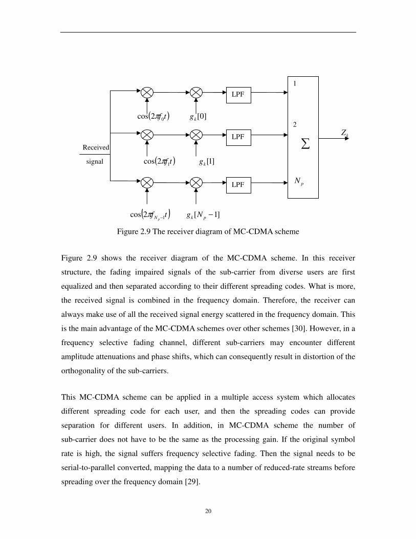
Figure 2.9 The receiver diagram of MC-CDMA scheme

Figure 2.9 shows the receiver diagram of the MC-CDMA scheme. In this receiver

structure, the fading impaired signals of the sub-carrier from diverse users are first

equalized and then separated according to their different spreading codes. What is more,

the received signal is combined in the frequency domain. Therefore, the receiver can

always make use of all the received signal energy scattered in the frequency domain. This

is the main advantage of the MC-CDMA schemes over other schemes [30]. However, in a

frequency selective fading channel, different sub-carriers may encounter different

amplitude attenuations and phase shifts, which can consequently result in distortion of the

orthogonality of the sub-carriers.

This MC-CDMA scheme can be applied in a multiple access system which allocates

different spreading code for each user, and then the spreading codes can provide

separation for different users. In addition, in MC-CDMA scheme the number of

sub-carrier does not have to be the same as the processing gain. If the original symbol

rate is high, the signal suffers frequency selective fading. Then the signal needs to be

serial-to-parallel converted, mapping the data to a number of reduced-rate streams before

spreading over the frequency domain [29].

LPF

LPF

LPF

1

2

∑

pN

21

2.3.2 MC-DS-CDMA scheme

( )tck ( )tf12cos π ( )tsk

Data

( )tck ( )tf22cos π

( )tck ( )tfpN 12cos −π

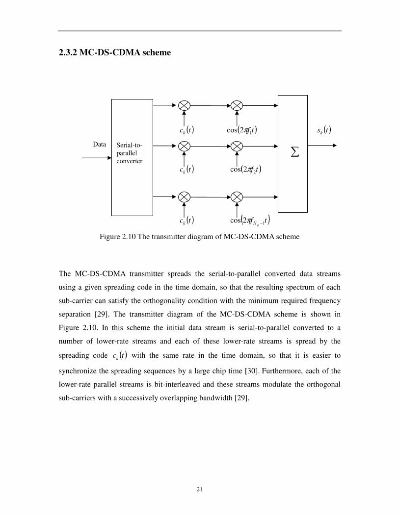
Figure 2.10 The transmitter diagram of MC-DS-CDMA scheme

The MC-DS-CDMA transmitter spreads the serial-to-parallel converted data streams

using a given spreading code in the time domain, so that the resulting spectrum of each

sub-carrier can satisfy the orthogonality condition with the minimum required frequency

separation [29]. The transmitter diagram of the MC-DS-CDMA scheme is shown in

Figure 2.10. In this scheme the initial data stream is serial-to-parallel converted to a

number of lower-rate streams and each of these lower-rate streams is spread by the

spreading code ( )tck with the same rate in the time domain, so that it is easier to

synchronize the spreading sequences by a large chip time [30]. Furthermore, each of the

lower-rate parallel streams is bit-interleaved and these streams modulate the orthogonal

sub-carriers with a successively overlapping bandwidth [29].

Serial-to-

parallel

converter

∑

22

( )tf02cos π ( )tck

Received

signal kZ

( )tf12cos π ( )tck

( )tfpN 12cos −π ( )tck

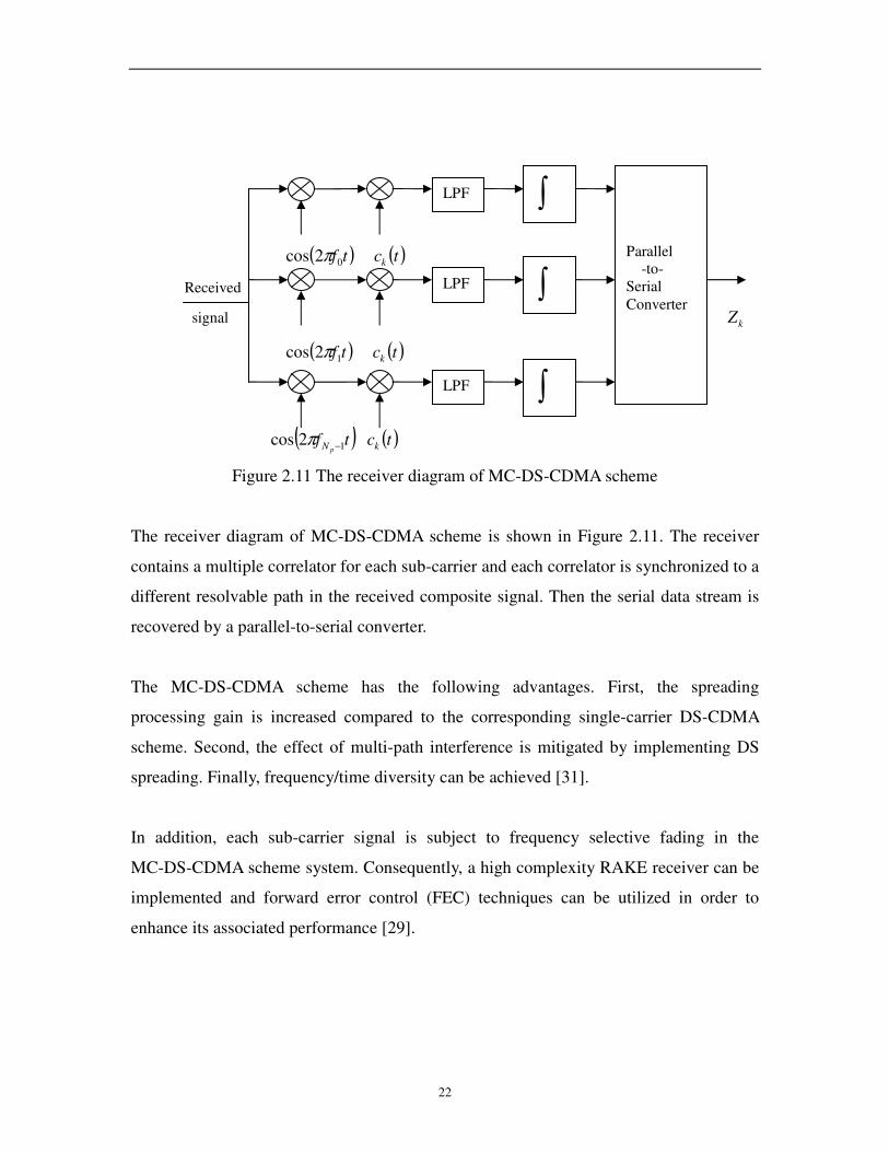
Figure 2.11 The receiver diagram of MC-DS-CDMA scheme

The receiver diagram of MC-DS-CDMA scheme is shown in Figure 2.11. The receiver

contains a multiple correlator for each sub-carrier and each correlator is synchronized to a

different resolvable path in the received composite signal. Then the serial data stream is

recovered by a parallel-to-serial converter.

The MC-DS-CDMA scheme has the following advantages. First, the spreading

processing gain is increased compared to the corresponding single-carrier DS-CDMA

scheme. Second, the effect of multi-path interference is mitigated by implementing DS

spreading. Finally, frequency/time diversity can be achieved [31].

In addition, each sub-carrier signal is subject to frequency selective fading in the

MC-DS-CDMA scheme system. Consequently, a high complexity RAKE receiver can be

implemented and forward error control (FEC) techniques can be utilized in order to

enhance its associated performance [29].

LPF

LPF

LPF

Parallel

-to-

Serial

Converter ∫

∫

∫

23

2.3.3 MT-DS-CDMA scheme

( )tck ( )tf12cos π ( )tsk

Data

( )tck ( )tf22cos π

( )tck ( )tfpN 12cos −π

Figure 2.12 the transmitter diagram of MT-DS-CDMA scheme

The MT-DS-CDMA transmitter spreads the serial-to-parallel converted data streams

using a given spreading code in the time domain so that the spectrum of each sub-carrier

before spreading operation can satisfy the orthogonality condition with the minimum

frequency separation [29]. Therefore, the resulting spectrum of each sub-carrier no longer

satisfies the orthogonality condition and strong spectral overlap exists among the

different sub-carrier signals after DS spreading [30]. Figure 2.12 shows the transmitter

diagram of MT-DS-CDMA scheme. In this scheme, the original binary data stream is

firstly serial-to-parallel converted to parallel sub-streams and then spectrum spreading

occurs in multiplying parallel sub-streams with spreading code ( )tck . Finally, the

MT-DS-CDMA signal is generated by adding all of the different sub-carriers’ signals.

Serial-to-

parallel

converter

∑

24

( )tf02cos π

Received

signal kZ

( )tf12cos π

( )tfpN 12cos −π

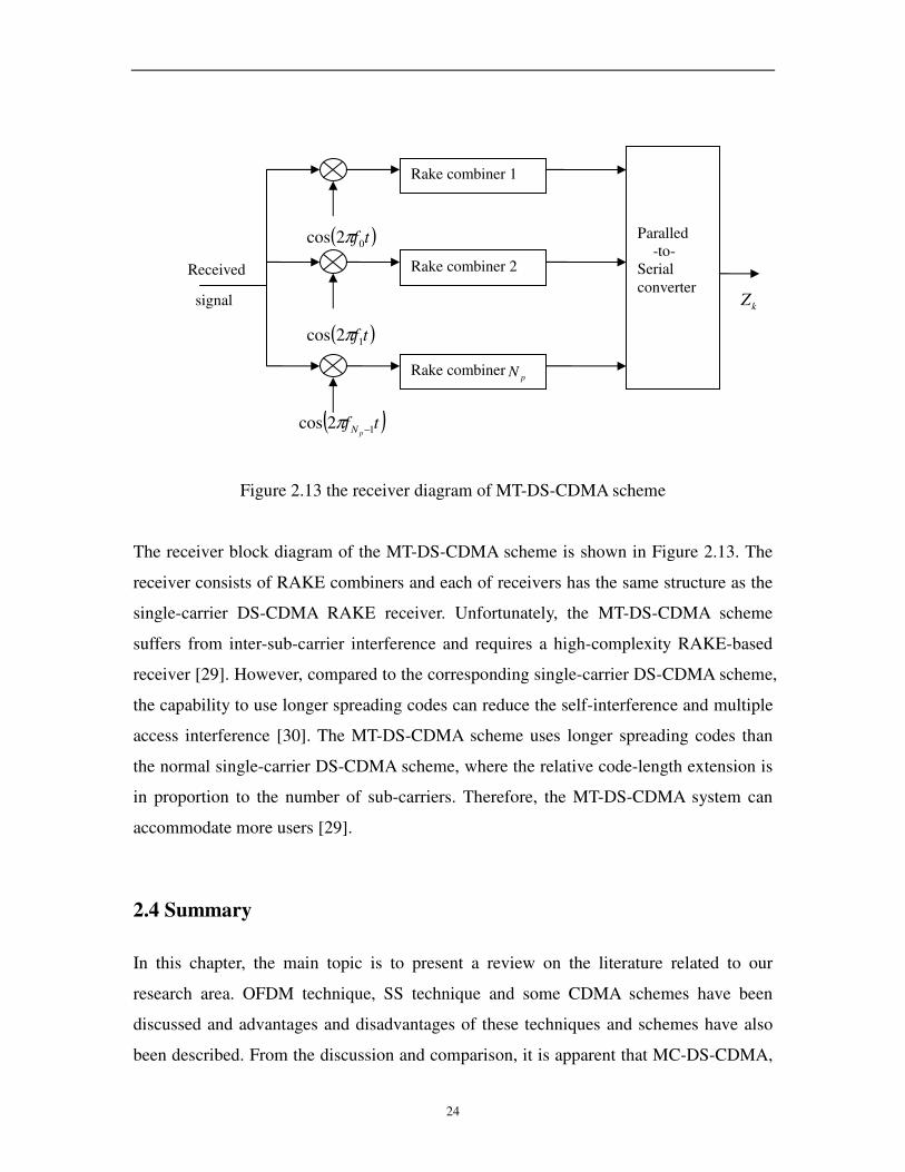
Figure 2.13 the receiver diagram of MT-DS-CDMA scheme

The receiver block diagram of the MT-DS-CDMA scheme is shown in Figure 2.13. The

receiver consists of RAKE combiners and each of receivers has the same structure as the

single-carrier DS-CDMA RAKE receiver. Unfortunately, the MT-DS-CDMA scheme

suffers from inter-sub-carrier interference and requires a high-complexity RAKE-based

receiver [29]. However, compared to the corresponding single-carrier DS-CDMA scheme,

the capability to use longer spreading codes can reduce the self-interference and multiple

access interference [30]. The MT-DS-CDMA scheme uses longer spreading codes than

the normal single-carrier DS-CDMA scheme, where the relative code-length extension is

in proportion to the number of sub-carriers. Therefore, the MT-DS-CDMA system can

accommodate more users [29].

2.4 Summary

In this chapter, the main topic is to present a review on the literature related to our

research area. OFDM technique, SS technique and some CDMA schemes have been

discussed and advantages and disadvantages of these techniques and schemes have also

been described. From the discussion and comparison, it is apparent that MC-DS-CDMA,

Rake combiner 1

Paralled

-to-

Serial

converter

Rake combiner 2

Rake combinerpN

25

which is a combination of OFDM and SS technique, is among the very strong contenders

for the fourth-generation (4G) wireless systems.

26

3. Implementation of the MC-DS-CDMA system

3.0 Introduction

MC-DS-CDMA that is a technique of combination of multi-carrier modulation and

spread-spectrum has recently drawn widespread attention due to its potential for high

speed transmission and its effectiveness in mitigating the effects of dispersive multi-path

fading channels [32] and in combating various kinds of interferences. In this section, we

simulate a four-user MC-DS-CDMA system using simulink in Matlab with the effect of

AWGN channel and multi-path Rayleigh fading channel.

The block diagram of the MC-DS-CDMA system for four mobile users is shown in Figure

3.1. In this system, the transmitted downlink data for four different users is spread

respectively using the orthogonal spreading code sequence assigned to each user and then

summed together and transmitted simultaneously through the same channel. Then the data

stream is recovered correctly by despreading using the spreading code sequence of each

user at receiver side. More details are explained in the following sections.

27

Zero-Order

Hold

Walsh Code

Generator

Walsh Code

Generator1

Unbuffer

Out1

Out2

Subsystem4

Out1

Out2

Subsystem3

Out1

Out2

Subsystem1

Out1

Out2

Subsystem

U U(E)

Slector1

U U(E)

Selector2

Reshape

Reshape

Repeat

Rx

Repeat2Product1

Product

Multipath

Rayleigh Fading

Multipath Rayleigh

Fading Channel1

1

u

Math

Function

MATLAB

Function

MATLAB Fcn2

MATLAB

Function

MATLAB Fcn1

MATLAB

Function

MATLAB Fcn

-5

Z

Integer Delay

1/4

Gain

To

Frame

Frame Status

Conversion2

To

Frame

Frame Status

Conversion1

FFT

FFT

Error Rate

Calculation

Tx

Rx

Error Rate

Calculation3

Error Rate

Calculation

Tx

Rx

Error Rate

Calculation2

Error Rate

Calculation

Tx

Rx

Error Rate

Calculation1

Error Rate

Calculation

Tx

Rx

Error Rate

Calculation

0

Display8

0

Display3

0

Display2

0

Display1

Buffer

BPSK

BPSK

Demodulator

Baseband

AWGN

AWGN

Channel1

Figure 3.1 Block diagram of four-user MC-DS-CDMA system

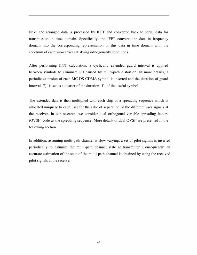
3.1 Transmitter

The block diagram of the MC-DS-CDMA transmitter for a single user is shown in Figure

3.2. In MC-DS-CDMA system, the original input data is first converted from serial stream

into parallel stream and then modulated by the binary phase shift keying (BPSK)

modulator. In order to reduce aliasing in D/A conversion, sub-carriers at or near the

Nyquist frequency need to be avoided by inserting zeros. Assuming 16 samples, [1 2 3 4 5

6 7 8 9 10 11 12 13 14 15 16], are selected to do IFFT calculation, they need to be

arranged as [0 2 3 4 5 6 7 0 0 0 11 12 13 14 15 16] before IFFT calculation.

28

Next, the arranged data is processed by IFFT and converted back to serial data for

transmission in time domain. Specifically, the IFFT converts the data in frequency

domain into the corresponding representation of this data in time domain with the

spectrum of each sub-carrier satisfying orthogonality conditions.

After performing IFFT calculation, a cyclically extended guard interval is applied

between symbols to eliminate ISI caused by multi-path distortion. In more details, a

periodic extension of each MC-DS-CDMA symbol is inserted and the duration of guard

interval g

T is set as a quarter of the duration T of the useful symbol.

The extended data is then multiplied with each chip of a spreading sequence which is

allocated uniquely to each user for the sake of separation of the different user signals at

the receiver. In our research, we consider dual orthogonal variable spreading factors

(OVSF) code as the spreading sequence. More details of dual OVSF are presented in the

following section.

In addition, assuming multi-path channel is slow varying, a set of pilot signals is inserted

periodically to estimate the multi-path channel state at transmitter. Consequently, an

accurate estimation of the state of the multi-path channel is obtained by using the received

pilot signals at the receiver.

29

Figure 3.2 Block diagram of MC-DS-CDMA transmitter for a single user

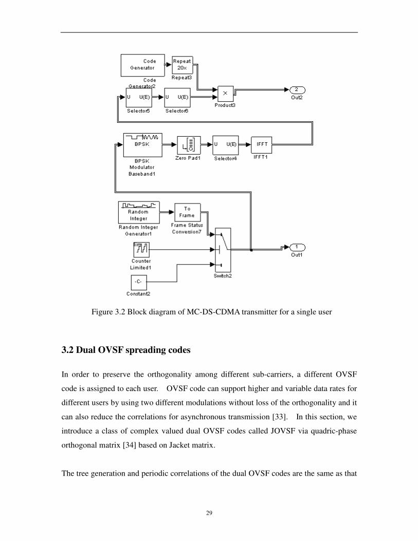
3.2 Dual OVSF spreading codes

In order to preserve the orthogonality among different sub-carriers, a different OVSF

code is assigned to each user. OVSF code can support higher and variable data rates for

different users by using two different modulations without loss of the orthogonality and it

can also reduce the correlations for asynchronous transmission [33]. In this section, we

introduce a class of complex valued dual OVSF codes called JOVSF via quadric-phase

orthogonal matrix [34] based on Jacket matrix.

The tree generation and periodic correlations of the dual OVSF codes are the same as that

30

of the conventional binary OVSF codes based on Hadamard, which is referred to as

HOVSF, but the seeds of those codes are different [33]. The dual OVSF can be

decomposed as two parts, one is conventional HOVSF, and the other is the JOVSF from

Jacket matrix [33].

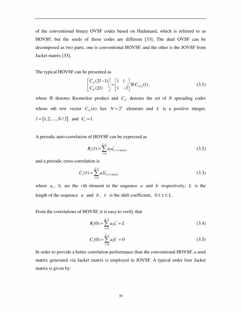
The typical HOVSF can be presented as

2

(2 1) 1 1( )

(2 ) 1 1

N

N

N

C lC l

C l

− = ⊗ −

, (3.1)

where ⊗ denotes Kronecker product and N

C denotes the set of N spreading codes

whose nth row vector ( )N

C n has 2kN = elements and k is a positive integer,

{ }1,2,...., / 2l N= and 11 =C .

A periodic auto-correlation of HOVSF can be expressed as

∑−

=+=

1

0

*

mod)()(L

i

Liii aaR ττ (3.2)

and a periodic cross-correlation is

∑−

=+=

1

0

*

mod)()(L

i

Liii baC ττ (3.3)

where ia , ib are the i th element in the sequence a and b respectively; L is the

length of the sequence a and b , τ is the shift coefficient, L≤≤τ0 .

From the correlations of HOVSF, it is easy to verify that

LaaRL

i

iii ==∑−

=

1

0

*)0( (3.4)

0)0(1

0

* ==∑−

=

L

i

iii baC (3.5)

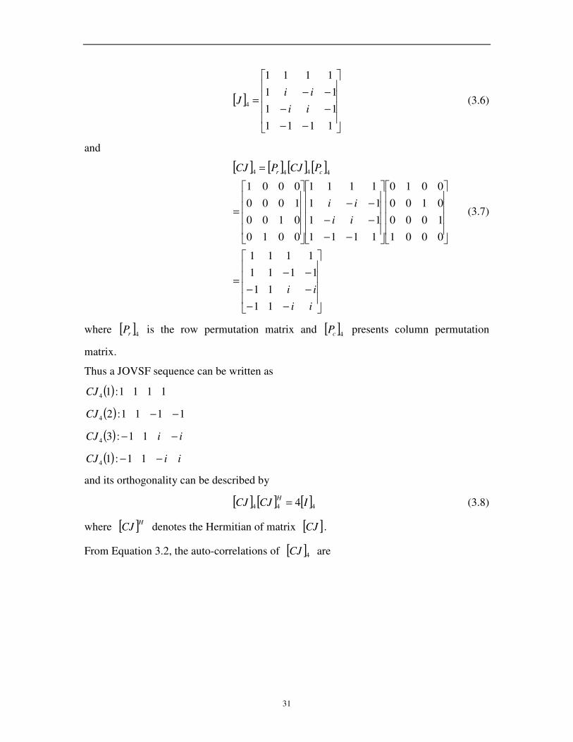
In order to provide a better correlation performance than the conventional HOVSF, a seed

matrix generated via Jacket matrix is employed in JOVSF. A typical order four Jacket

matrix is given by:

31

[ ]

−−

−−

−−=

1111

11

11

1111

4ii

iiJ (3.6)

and

[ ] [ ] [ ] [ ]

−−

−−

−−=

−−

−−

−−

=

=

ii

ii

ii

ii

PCJPCJ cr

11

11

1111

1111

0001

1000

0100

0010

1111

11

11

1111

0010

0100

1000

0001

4444

(3.7)

where [ ]4rP is the row permutation matrix and [ ]

4cP presents column permutation

matrix.

Thus a JOVSF sequence can be written as

( ) 1111:14CJ

( ) 1111:24 −−CJ

( ) iiCJ −− 11:34

( ) iiCJ −− 11:14

and its orthogonality can be described by

[ ] [ ] [ ]444 4 ICJCJH

= (3.8)

where [ ]HCJ denotes the Hermitian of matrix [ ]CJ .

From Equation 3.2, the auto-correlations of [ ]4CJ are

32

From Equation 3.3, the cross-correlations of [ ]4CJ are

Starting from [ ]4CJ , we can derive a similar formula from Equation 3.1,

)(11

11

)2(

)12(4

8

8lCJ

lCJ

lCJ⊗

−=

− (3.9)

Thus length-8 JOVSF sequence is

33

The auto-correlations of [ ]8CJ are

The cross-correlations of [ ]8CJ are

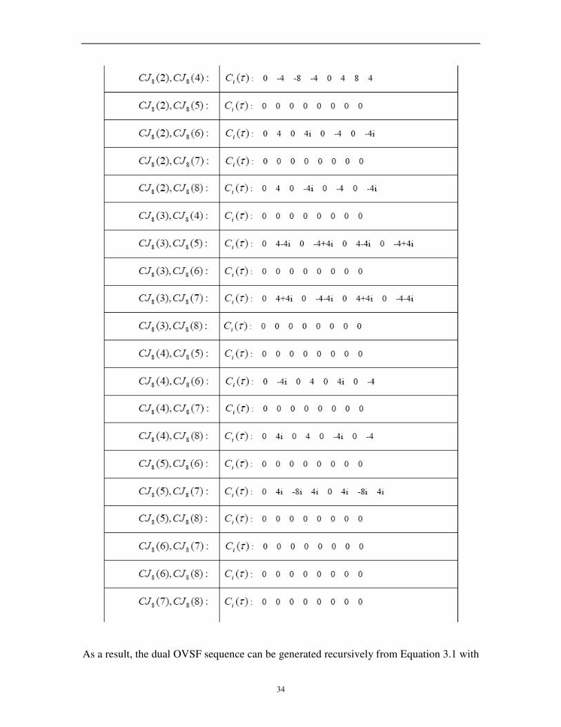
34

As a result, the dual OVSF sequence can be generated recursively from Equation 3.1 with

35

any length L as a power of 2 and the periodic correlations of the dual OVSF can be

derived from Equation 3.2 and 3.3. The advantage of dual OVSF is demonstrated in the

following comparison of peak correlation values with HOVSF [33].

Autocorrelation Crosscorrelation

HOVSF Dual OVSF HOVSF Dual OVSF

Peak value 4 4 4 4

Number of

peak values 12 8 2 1

Table 3.1 Comparison of peak correlation values: length-4 HOVSF AND dual OVSF

codes

Autocorrelation Crosscorrelation

HOVSF Dual OVSF HOVSF Dual OVSF

Peak value 8 8 8 8

Number of

peak values 32 28 8 4

Table 3.2 Comparison of peak correlation values: length-8 HOVSF AND dual OVSF

codes

3.3 Channel simulation

A crucial requirement for the MC-DS-CDMA system is to describe characteristics of

wireless channel accurately. Statistical characteristics of the wireless channel heavily

depend on the physical multi-path propagation environment [35]. Multi-path is a salient

feature in high-speed wireless communication. It results in transmitted radio signals’

reflecting from terrain features such as trees or mountains, or obstructions such as people,

vehicles or buildings and then reaching receiver at different times by two or more paths.

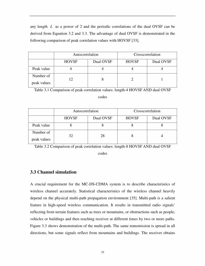
Figure 3.3 shows demonstration of the multi-path. The same transmission is spread in all

directions, but some signals reflect from mountains and buildings. The receiver obtains

36

more than one copy of the original signal. Since the indirect path takes more time to

travel to the receiver, the delayed copies of the original signal interfere with the direct

signal and the receiver can not decode the original signal correctly [36].

Figure 3.3: Multi-path Demonstration [36]

The channel simulation is characterized by AWGN channel simulation and multi-path

Rayleigh fading channel simulation in our research. AWGN channel is simulated by

adding random numbers with Gaussian distribution to the transmitted signal as

background noise. Multi-path Rayleigh fading channel simulation involves multiplying

the transmitted signal by channel gain vector and adding delayed copies of the

transmitted signal in propagation. This simulates the problem in wireless communication

when the signal propagates on many paths [36]. Furthermore, parameters of channel gain

and delay time from a set of 6 typical channels called modified Stanford University

Interim (SUI) Channel Models are applied to test the performance of MC-DS-CDMA

system in this research and the parameters are presented as Table 3.3- Table 3.8 [37]:

37

SUI-1 Channel

Tap 1 Tap 2 Tap 3 Units

Delay 0 0.4 0.9 sµ

Channel gain 0 -15 -20 dB

Table 3.3 parameters of SUI-1

SUI-2 Channel


Delay 0 0.4 1.1 sµ



SUI-3 Channel


Delay 0 0.4 0.9 sµ



SUI-4 Channel


Delay 0 1.4 4 sµ



SUI-5 Channel


Delay 0 4 10 sµ



38

SUI-6 Channel


Delay 0 14 20 sµ



Figure 3.4 show the channel model of the MC-DS-CDMA system. Multi-path Rayleigh

fading channel implements the simulation of multi-path and fading effects and AWGN

channel adds white Gaussian noise effect.

Unbuffer

Multipath

Rayleigh Fading

Multipath Rayleigh

Fading Channel1

To

Frame

Frame Status

Conversion1Buffer

AWGN

AWGN

Channel1

Figure 3.4 Block diagram of MC-DS-CDMA channel model

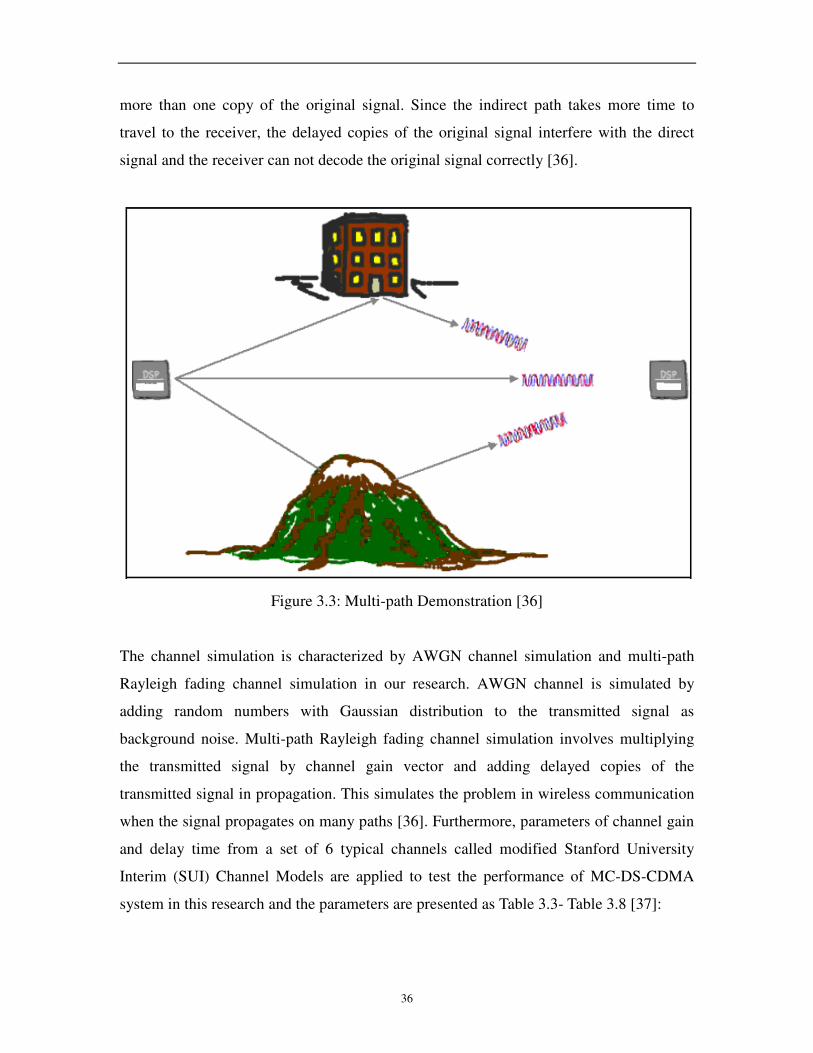
3.4 Receiver

The receiver implements the inverse process of the transmitter. First, the received signal

is converted from serial into parallel stream and decoded using users’ OVSF code index.

Accordingly, the receiver can identify the data stream from different users. Next, the

guard interval is removed. Then the FFT calculation is applied and the inserted zeros are

removed from data stream. After performing the system delay, the channel gain of

multi-path channel is calculated according to the received pilot data. The effect of

multi-path fading channel is eliminated by multiplying received data by reciprocal of the

channel gain. Finally, BPSK demodulation is applied. Thus the original data can be

recovered. Figure 3.5 presents the receiver of the MC-DS-CDMA system.

39

Figure 3.5 Block diagram of MC-DS-CDMA receiver

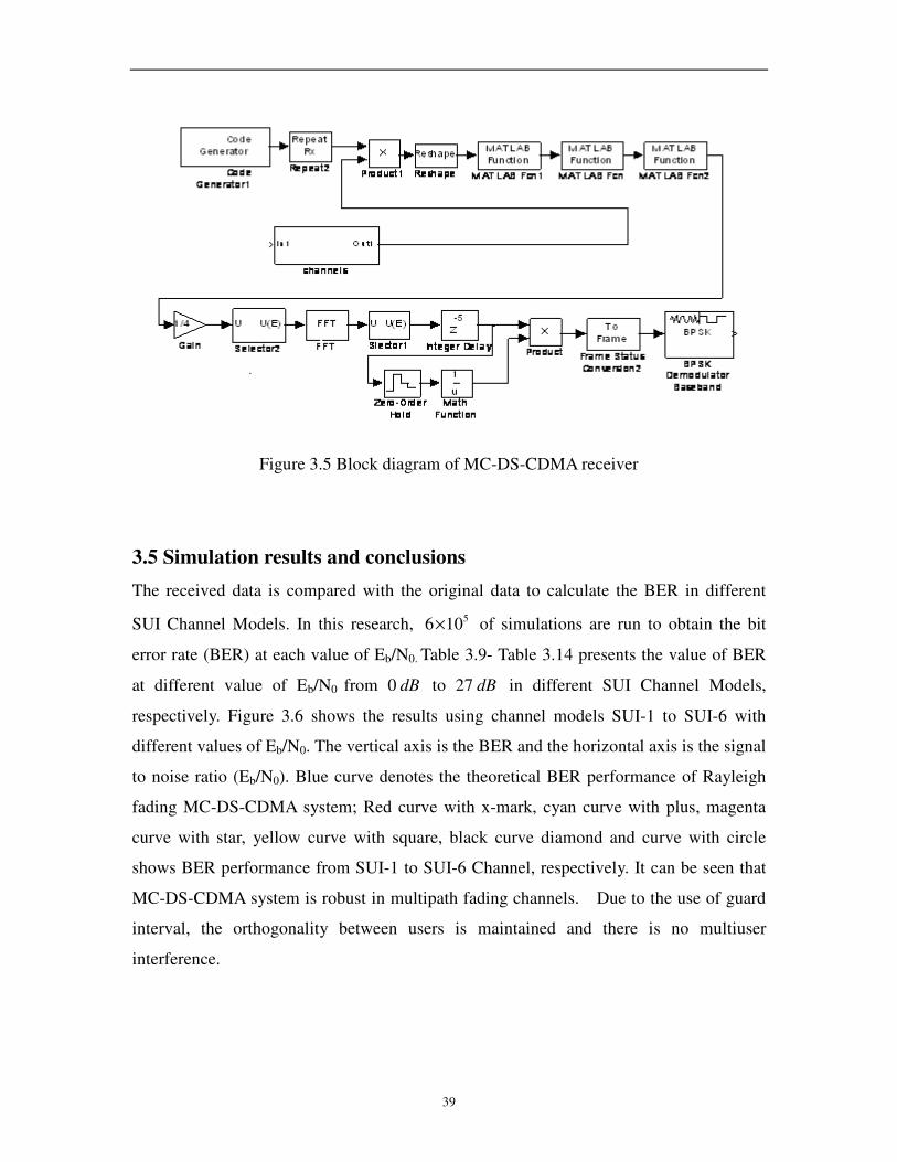
3.5 Simulation results and conclusions

The received data is compared with the original data to calculate the BER in different

SUI Channel Models. In this research, 5106× of simulations are run to obtain the bit

error rate (BER) at each value of Eb/N0. Table 3.9- Table 3.14 presents the value of BER

at different value of Eb/N0 from 0 dB to 27 dB in different SUI Channel Models,

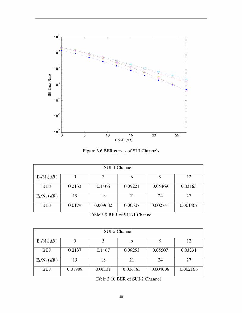
respectively. Figure 3.6 shows the results using channel models SUI-1 to SUI-6 with

different values of Eb/N0. The vertical axis is the BER and the horizontal axis is the signal

to noise ratio (Eb/N0). Blue curve denotes the theoretical BER performance of Rayleigh

fading MC-DS-CDMA system; Red curve with x-mark, cyan curve with plus, magenta

curve with star, yellow curve with square, black curve diamond and curve with circle

shows BER performance from SUI-1 to SUI-6 Channel, respectively. It can be seen that

MC-DS-CDMA system is robust in multipath fading channels. Due to the use of guard

interval, the orthogonality between users is maintained and there is no multiuser

interference.

40

0 5 10 15 20 2510

-6

10-5

10-4

10-3

10-2

10-1

100

EbN0 (dB)

Bit E

rror

Rate

Figure 3.6 BER curves of SUI Channels

SUI-1 Channel

Eb/N0( dB ) 0 3 6 9 12

BER 0.2133 0.1466 0.09221 0.05469 0.03163

Eb/N0 ( dB ) 15 18 21 24 27

BER 0.0179 0.009682 0.00507 0.002741 0.001467

Table 3.9 BER of SUI-1 Channel

SUI-2 Channel

Eb/N0( dB ) 0 3 6 9 12

BER 0.2137 0.1467 0.09253 0.05507 0.03231

Eb/N0 ( dB ) 15 18 21 24 27

BER 0.01909 0.01138 0.006783 0.004006 0.002166


41

SUI-3 Channel

Eb/N0( dB ) 0 3 6 9 12

BER 0.2092 0.14 0.08425 0.04678 0.02462

Eb/N0 ( dB ) 15 18 21 24 27

BER 0.01239 0.005925 0.002649 0.001004 0.0004251


SUI-4 Channel

Eb/N0( dB ) 0 3 6 9 12

BER 0.2081 0.1387 0.08264 0.04573 0.0239

Eb/N0 ( dB ) 15 18 21 24 27

BER 0.01211 0.00614 0.002944 0.001212 0.0004901


SUI-5Channel

Eb/N0( dB ) 0 3 6 9 12

BER 0.2092 0.14 0.06307 0.04678 0.02464

Eb/N0 ( dB ) 15 18 21 24 27

BER 0.01239 0.005926 0.002651 0.001009 0.0004201


SUI-6 Channel

Eb/N0( dB ) 0 3 6 9 12

BER 0.2127 0.146 0.0914 0.0538 0.03116

Eb/N0 ( dB ) 15 18 21 24 27

BER 0.01811 0.01064 0.006073 0.003276 0.0087


42

4. BER performance analysis on the effect of timing jitter

4.0 Introduction

The MC-DS-CDMA systems are more sensitive to errors in sampling time which is

generally called timing jitter than single-carrier systems due to the use of large number of

sub-carriers. Timing jitter caused by mismatch of sampling time between the transmitter

and receiver degrades performance of the system seriously because timing jitter destroys

orthogonality among sub-carriers and results in ICI. To avoid the degradation associated

with a timing jitter, the timing jitter should be corrected by a proper timing

synchronization algorithm. It has been shown that the performance degradation for the

MC-DS-CDMA system caused by timing jitter is independent of the number of

sub-carriers, of the spreading factor, and of the spectral contents of the jitter, but only

depends on the timing jitter variance [38].

In this section, the investigation of effects of timing jitter on the MC-DS-CDMA system is

introduced. In particular, we will pay more attention on the BER performance of the

MC-DS-CDMA system due to the timing jitter both in additive white Gaussian noise

(AWGN) channel and multi-path Rayleigh fading channel. We firstly formulate the

analytical expressions for the MC-DS-CDMA signals in presence of the timing jitter and

then compare BER performance of the ideal MC-DS-CDMA system with the BER

performances affected by timing jitters when the timing jitters are independent and

dependent, respectively.

4.1 Problem formulation

In MC-DS-CDMA communication systems, the complex data symbols to be transmitted

are first split into lower rate symbol sequences, and then each of these lower rate symbol

sequences modulates a different sub-carrier of the orthogonal multi-carrier system. The

received MC-DS-CDMA signal over the useful symbol duration of s

T at

43

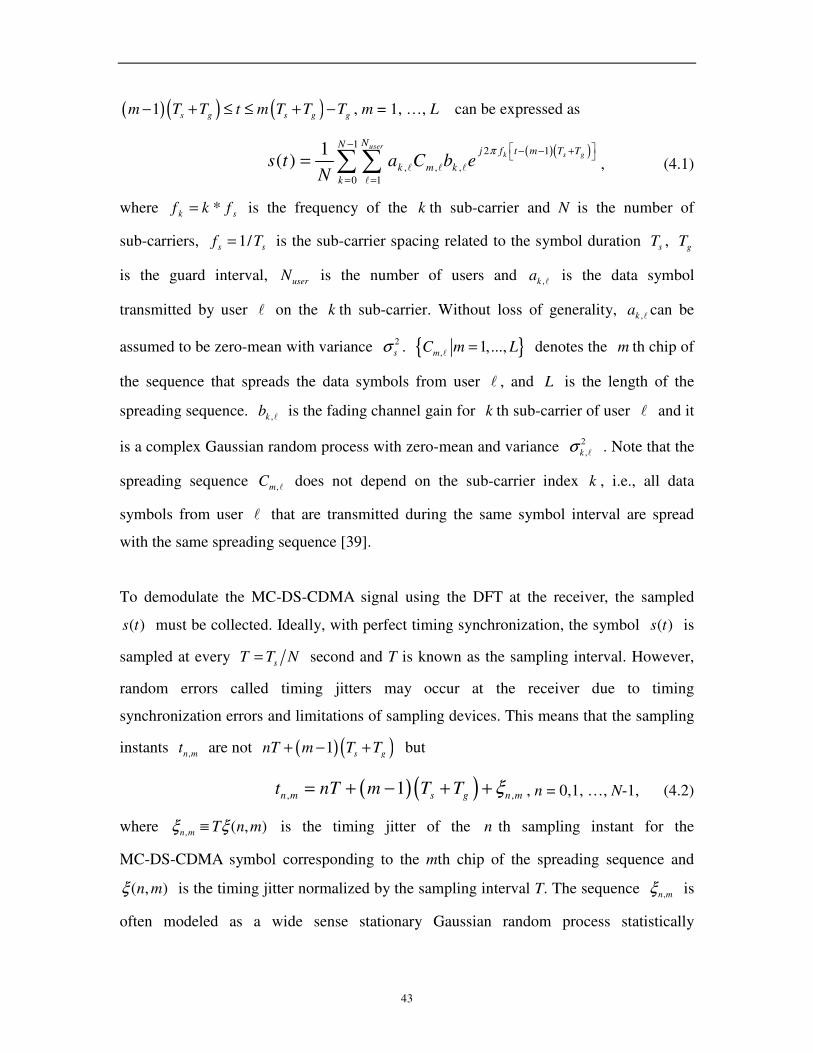
( )( ) ( )1s g s g g

m T T t m T T T− + ≤ ≤ + − , m = 1, …, L can be expressed as

( )( )12 1

, , ,

0 1

1( )

userk s g

NNj f t m T T

k m k

k

s t a C b eN

π− − − +

= =

= ∑∑ l l l

l

, (4.1)

where sk fkf *= is the frequency of the k th sub-carrier and N is the number of

sub-carriers, ss Tf /1= is the sub-carrier spacing related to the symbol duration sT , g

T

is the guard interval, userN is the number of users and l,ka is the data symbol

transmitted by user l on the k th sub-carrier. Without loss of generality, l,ka can be

assumed to be zero-mean with variance 2

sσ . { }, 1,...,m

C m L=l

denotes the m th chip of

the sequence that spreads the data symbols from user l , and L is the length of the

spreading sequence. l,kb is the fading channel gain for k th sub-carrier of user l and it

is a complex Gaussian random process with zero-mean and variance 2

,kσl . Note that the

spreading sequence l,mC does not depend on the sub-carrier index k , i.e., all data

symbols from user l that are transmitted during the same symbol interval are spread

with the same spreading sequence [39].

To demodulate the MC-DS-CDMA signal using the DFT at the receiver, the sampled

)(ts must be collected. Ideally, with perfect timing synchronization, the symbol )(ts is

sampled at every s

T T N= second and T is known as the sampling interval. However,

random errors called timing jitters may occur at the receiver due to timing

synchronization errors and limitations of sampling devices. This means that the sampling

instants ,n mt are not ( ) ( )1

s gnT m T T+ − + but

( )( ), ,1n m s g n m

t nT m T T ξ= + − + + , n = 0,1, …, N-1, (4.2)

where ),(, mnTmn ξξ ≡ is the timing jitter of the n th sampling instant for the

MC-DS-CDMA symbol corresponding to the mth chip of the spreading sequence and

( , )n mξ is the timing jitter normalized by the sampling interval T. The sequence mn,ξ is

often modeled as a wide sense stationary Gaussian random process statistically

44

independent of the input signal with zero mean and variance 2

Jσ [40]. Therefore,

without loss of generality, the actual sampled signal can be expressed as

( )( ) ,

12 ( )

, , , , ,

0 1

1 2 [ ( , )]

, , ,

0 1

1 2 [ ( , )]

, , ,

0 1

1( 1 )

1

1

user

k n m

user

user

NNj f nT

n m s g n m k m k

k

kNN j nT T n mTN

k m k

k

kNN j n n mN

k m k

k

x s nT m T T a C b eN

a C b eN

a C b eN

π ξ

π ξ

π ξ

ξ−

+

= =

− +

= =

− +

= =

= + − + + =

=

=

∑∑

∑∑

∑∑

l l l

l

l l l

l

l l l

l

. (4.3)

With the increase of sampling rate, the timing jitters at adjacent samples may become

more correlated. Correlation model of timing jitters is described as Gaussian-shaped or

exponential in [40, 41]. To analyze the effects of different degrees of correlation between

sampling timing errors on the performance of MC-DS-CDMA system, we adopt the

following discrete autocorrelation function of timing jitter [41]

n

J an2

)( σρ = , 1≤a , (4.4)

where 2

Jσ is the variance of timing jitter with zero-mean; a can be described as the

level of correlation between different timing jitters. For instance, 1=a corresponds to a

constant offset on the sampling instants, while 0=a corresponds to uncorrelated timing

jitter on different samples [41].

4.2 ICI due to timing jitter

The ICI caused by the timing jitter in the MC-DS-CDMA system based on the AWGN

channel and the multi-path Rayleigh fading channel is analyzed in this section.

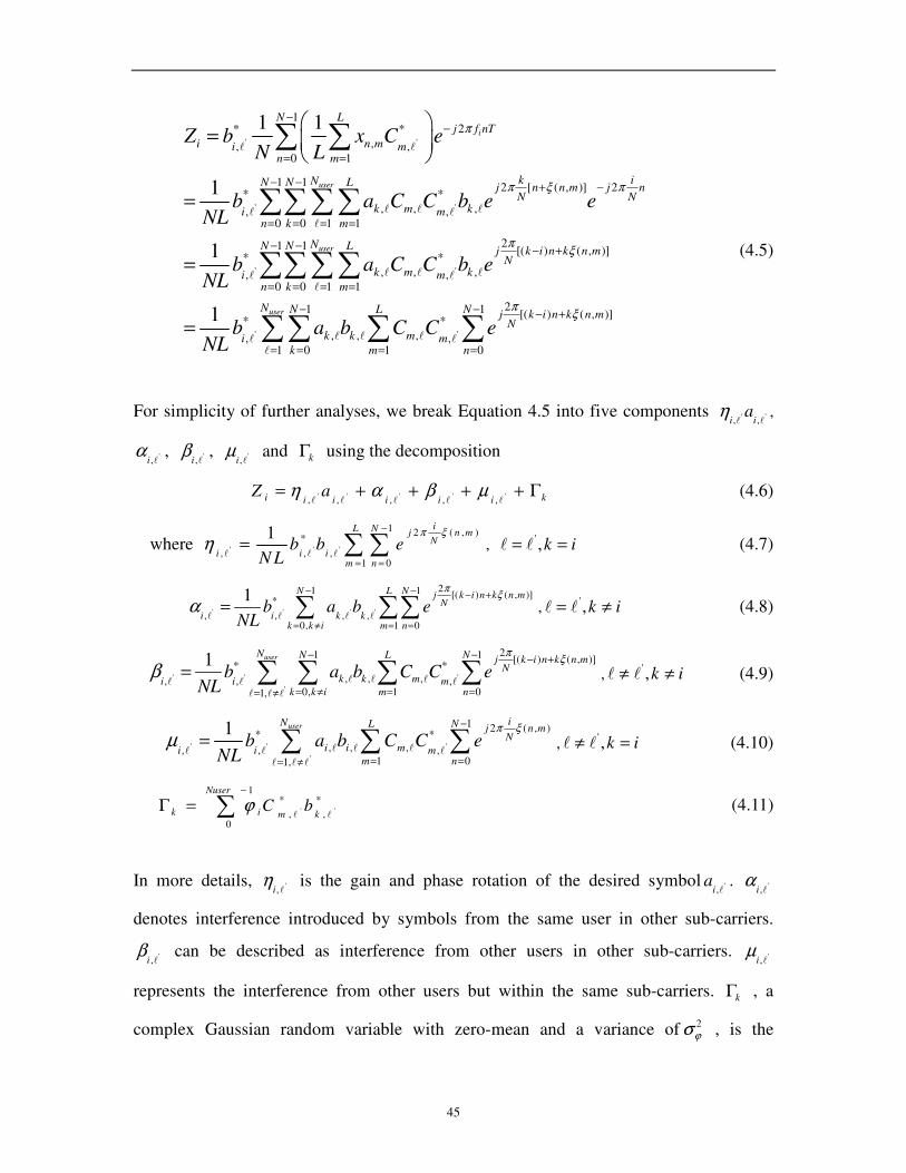
Using Equation 4.3, the decision variable Zi for the data symbol carried by the ith

sub-carrier of user 'l can be obtained from the received signal samples after

despreading as

45

' '

' '

' '

12* *

,, ,0 1

1 1 2 [ ( , )] 2* *

, , ,, ,0 0 1 1

21 [( ) ( , )]* *

, , ,, ,0 1 1

1 1

1

1

i

user

user

N Lj f nT

i n mi mn m

k iNN N L j n n m j nN N

k m ki mn k m

NN L j k i n k n mN

k m ki mk m

Z b x C eN L

b a C C b e eNL

b a C C b eNL

π

π ξ π

πξ

−−

= =

− − + −

= = = =

− − +

= = =

=

=

=

∑ ∑

∑∑∑∑

∑∑∑

l l

l l ll l

l

l l ll l

l

' '

1

0

21 1 [( ) ( , )]* *

, , ,, ,1 0 1 0

1 user

N

n

N N L N j k i n k n mN

k k mi mk m n

b a b C C eNL

πξ

−

=

− − − +

= = = =

=

∑

∑∑ ∑ ∑l l ll l

l

(4.5)

For simplicity of further analyses, we break Equation 4.5 into five components '',, ll ii

aη ,

',li

α , ',li

β , ',li

µ and kΓ using the decomposition

kiiiiii aZ Γ++++= ''''',,,,, lllll

µβαη (4.6)

where ' ' '

1 2 ( , )*

, , ,1 0

1iL N j n mN

i i im n

b b eN L

π ξ

η−

= =

= ∑ ∑l l l, ik == ,

'll (4.7)

' ' ' '

21 1 [( ) ( , )]*

, , , ,0, 1 0

1 N L N j k i n k n mN

i i k kk k i m n

b a b eNL

πξ

α− − − +

= ≠ = =

= ∑ ∑∑l l l l, ik ≠= ,

'll (4.8)

' ' '

'

21 1 [( ) ( , )]* *

, , ,, , ,0, 1 01,

1 userN N L N j k i n k n mN

k k mi i mk k i m n

b a b C C eNL

πξ

β− − − +

= ≠ = == ≠

= ∑ ∑ ∑ ∑l l ll l l

l l l

, ik ≠≠ ,'ll (4.9)

' ' '

'

1 2 ( , )* *

, , ,, , ,1 01,

1 user iN L N j n mN

i i mi i mm n

b a b C C eNL

π ξ

µ−

= == ≠

= ∑ ∑ ∑l l ll l l

l l l

, ik =≠ ,'ll (4.10)

*

,

1

0

*

, ''ll k

Nuser

mik bC∑−

=Γ ϕ (4.11)

In more details, ',li

η is the gain and phase rotation of the desired symbol ',li

a . ',li

α

denotes interference introduced by symbols from the same user in other sub-carriers.

',li

β can be described as interference from other users in other sub-carriers. ',li

µ

represents the interference from other users but within the same sub-carriers. kΓ , a

complex Gaussian random variable with zero-mean and a variance of2

ϕσ , is the

46

contribution from thermal noise and the real and the imaginary parts of kΓ can be

assumed independent and identically distributed; hence,

2

2

1)var(

2

1])[var(])[var( ϕσ=Γ=Γℑ=Γℜ kkk [42]. iϕ is a sample of the thermal noise.

Note that the symbolsl,ka ’s are assumed to be zero-mean. Therefore,

0)( ',

=li

aE

0)( ',

=li

E β

0)( ',

=li

E µ

Thus the variance of ',li

α , ',li

β , and ',li

µ can be written as following from Equation

4.8-4.10, respectively.

}1

*1

{

)()]([)()(

1

,0 1

1

0

)],()[(2

*

,,,

1

,0 1

1

0

)],()[(2

*

,,,

2

,

2

,

2

,,

'' ' '

'''''

''''''''''

''''

∑ ∑∑∑ ∑∑−

≠= =

−

=

+−−−

≠= =

−

=

+−

=

=−=

N

ikk

L

m

N

n

mnknikN

j

kkk

N

ikk

L

m

N

n

mnknikN

j

kkk

iiii

ebbaN

ebbaN

E

EEEVar

ξπ

ξπ

αααα

llllll

llll

(4.12)

}1

*

1

{

)()]([)()(

'''' ' ' '

'''''

'''''''''''''''

'

''

''''

,,1

1

,0 1

1

0

)],()[(2

*

,,

*

,,,

,1

1

,0 1

1

0

)],()[(2

*

,,

*

,,,

2

,

2

,

2

,,

∑ ∑ ∑ ∑

∑ ∑ ∑ ∑

≠≠=

−

≠= =

−

=

+−−

≠=

−

≠= =

−

=

+−

=

=−=

Nuser N

ikk

L

m

N

n

mnknikN

j

kkmmk

Nuser N

ikk

L

m

N

n

mnknikN

j

lklkmmk

iiii

ebbCCaN

ebbCCaN

E

EEEVar

lllll

lllll

lll

lll

llll

ξπ

ξπ

ββββ

(4.13)

}1

*1

{

)()]([)()(

'''' ' '

''

''''''''''''''

'

''

''''

,,1 1

1

0

),(2

*

,,

*

,,,,1 1

1

0

),(2

*

,,

*

,,,

2

,

2

,

2

,,

∑ ∑ ∑∑ ∑ ∑≠≠= =

−

=

−

≠= =

−

=

=

=−=

Nuser L

m

N

n

mnkN

j

mmkkk

Nuser L

m

N

n

mnkN

j

mmkkk

iiii

eCCbbaN

eCCbbaN

E

EEEVar

lllll

lllll

lll

lllll

llll

ξπ

ξπ

µµµµ

(4.14)

Therefore, conditional mean of demodulated signal iZ can be expressed as:

47

)(

)()()()()(

)()(

''

'''''

'''''

,,

,,,,,

,,,,,

ll

lllll

lllll

ii

kiiiii

kiiiiii

aE

EEEEaE

aEZE

η

µβαη

µβαη

=

Γ++++=

Γ++++=

(4.15)

Conditional variance of demodulated signal iZ can be expressed as:

2

,,,,,

,,,,,

,,,,,

)()()()(

)()()()()(

)()(

'''''

'''''

'''''

ϕσµβαη

µβαη

µβαη

++++=

Γ++++=

Γ++++=

lllll

lllll

lllll

iiiii

kiiiii

kiiiiii

VarVarVaraVar

VarVarVarVaraVar

aVarZVar

(4.16)

Finally, the bit error rate (BER) of the MC-DS-CDMA system can be calculated as [43]

))(2

)((*2/1

i

i

ZVar

ZEerfcBER = (4.17)

where the complimentary error function erfc is defined as

∫∞

−=iz

t

i dteZerfc22

)(π

)( iZVar is the variance of iZ and )( iZE is the mean value of iZ

4.2.1 ICI due to white timing jitter

When timing jitter is white, the correlation coefficient is expressed as:

≠

==

0,0

0,1)(

n

nnρ (4.18)

then the variance of ',li

α can be written as following from Equation 4.12,

48

}1

*1

{

)()]([)()(

1

,0 1

1

0

)],()[(2

*

,,,

1

,0 1

1

0

)],()[(2

*

,,,

2

,

2

,

2

,,

'' ' '

'''''

''''''''''

''''

∑ ∑∑∑ ∑∑−

≠= =

−

=

+−−−

≠= =

−

=

+−

=

=−=

N

ikk

L

m

N

n

mnknikN

j

kkk

N

ikk

L

m

N

n

mnknikN

j

kkk

iiii

ebbaN

ebbaN

E

EEEVar

ξπ

ξπ

αααα

llllll

llll

When ''''' ,,, ll ==== nnmmkk

2*22

2

21

02

2*22

2*

,

2

,

1

0 1

1

0

)],(),([))([(2

2

2

2*

,

2

,

1

0 1 1

1

0

1

0

)],(),([))([(2

2

2

)],()[(21

0 1 1

1

0

1

0

)],()[(2

*

,,

*

,,

2

,2,

***}*{

)()(}{

}{

}{1

)(

'''

'''

'''

' '

'''

''''

'

' '

'''''''''

kks

sN

k

kks

kk

N

k

L

m

N

n

mnmnknnikN

js

kk

N

k

L

m

L

m

N

n

N

n

mnmnknnikN

js

mnknikN

jN

k

L

m

L

m

N

n

N

n

mnknikN

j

kkkkki

L

N

NNLNLE

N

bEbEeEN

bbeEN

eebbbbaEN

Var

σσσ

σσσσ

σ

σ

α

ξξπ

ξξπ

ξπ

ξπ

=

==

=

=

=

∑

∑∑∑

∑∑∑∑∑

∑ ∑∑∑∑

−

=

−

= =

−

=

−+−−

−

= = =

−

=

−

=

−+−−

+−−−

= = =

−

=

−

=

+−

ll

ll

llllll

(4.19)

When ''''' ,,, ll =≠== nnmmkk

22

2

2

''

'22

2

2'

'''

' '

'''

''''

'

' '

'''''''''

41

0

1

12

2*22

1

0 1

1

0

1

,0

)](1[4

)])([(2

2

2*22

2*

,

2

,

1

0 1 1

1

0

1

0

)],(),([))([(2

2

2

)],()[(21

0 1 1

1

0

1

0

)],()[(2

*

,,

*

,,

2

,2,

])(2

cos[)(2

)()(}{

}{1

)(

J

J

kN

N

k

N

n

kks

N

k

L

m

N

n

N

nnn

nnkN

nnikN

jkks

kk

N

k

L

m

L

m

N

n

N

n

mnmnknnikN

js

mnknikN

jN

k

L

m

L

m

N

n

N

n

mnknikN

j

kkkkki

enikN

nNN

L

eeN

bEbEeEN

eebbbbaEN

Var

σπ

ρσππ

ξξπ

ξπ

ξπ

πσσσ

σσσ

σ

α

−−

=

−

=∆

−

= =

−

=

−

≠=

−−−−−

−

= = =

−

=

−

=

−+−−

+−−−

= = =

−

=

−

=

+−

∆−∆−=

=

=

=

∑∑

∑∑∑ ∑

∑∑∑∑∑

∑ ∑∑∑∑

ll

llllll

(4.20)

When ''''' ,,, ll ==≠= nnmmkk

49

∑∑

∑∑ ∑ ∑

∑∑∑∑∑

∑ ∑∑∑∑

−

=

−

=∆

−

−

= = ≠=

−

=

−−−

−

= = =

−

=

−

=

−+−−

+−−−

= = =

−

=

−

=

+−

∆−=

=

=

=

1

0

1

1

42*22

1

0 1 ,1

1

0

))]((1[4

2

2*22

2*

,

2

,

1

0 1 1

1

0

1

0

)],(),([))([(2

2

2

)],()[(21

0 1 1

1

0

1

0

)],()[(2

*

,,

*

,,

2

,2,

22

2

2

''

'22

2

2

'''

' '

'''

''''

'

' '

'''''''''

)(2

)()(}{

}{1

)(

N

k

L

m

kNkks

N

k

L

m

L

mmm

N

n

mmNkNkks

kk

N

k

L

m

L

m

N

n

N

n

mnmnknnikN

js

mnknikN

jN

k

L

m

L

m

N

n

N

n

mnknikN

j

kkkkki

J

J

emLN

eN

bEbEeEN

eebbbbaEN

Var

σπ

ρσπ

ξξπ

ξπ

ξπ

σσσ

σσσ

σ

α

ll

llllll

(4.21)

When ''''' ,,, ll =≠≠= nnmmkk

22

2

2

'' ''

''22

2

2'

'''

'' ''

'''

''''

'

' '

'''''''''

41

0

1

1

1

12

2*22

1

0 1 ,1

1

0

1

,0

)]]()([1[4

)])([(2

2

2*22

2*

,

2

,

1

0 1 ,1

1

0

1

,0

)],(),([)])([(2

2

2

)],()[(21

0 1 1

1

0

1

0

)],()[(2

*

,,

*

,,

2

,2,

])(2

cos[))((4

)()(}{

}{1

)(

J

J

kN

N

k

L

m

N

n

kks

N

k

L

m

L

mmm

N

n

N

nnn

nnmmNkN

nnikN

jkks

kk

N

k

L

m

L

mmm

N

n

N

nnn

mnmnknnikN

js

mnknikN

jN

k

L

m

L

m

N

n

N

n

mnknikN

j

kkkkki

enikN

mLnNN

eeN

bEbEeEN

eebbbbaEN

Var

σπ

ρσππ

ξξπ

ξπ

ξπ

πσσσ

σσσ

σ

α

−−

=

−

=∆

−

=∆

−

= = ≠=

−

=

−

≠=

−+−−−−−

−

= = ≠=

−

=

−

≠=

−+−−

+−−−

= = =

−

=

−

=

+−

∆−∆−∆−=

=

=

=

∑∑ ∑

∑∑ ∑ ∑ ∑

∑∑ ∑ ∑ ∑

∑ ∑∑∑∑

ll

llllll

(4.22)

When 'kk ≠ or '

ll ≠

0)( ',

=li

Var α

From Equation 4.13, the variance of ',li

β can be expressed as:

}1

*

1

{

)()]([)()(

'''' ' ' '

'''''

'''''''''''''''

'

''

''''

,,1

1

,0 1

1

0

)],()[(2

*

,,

*

,,,

,1

1

,0 1

1

0

)],()[(2

*

,,

*

,,,

2

,

2

,

2

,,

∑ ∑ ∑ ∑

∑ ∑ ∑ ∑

≠≠=

−

≠= =

−

=

+−−

≠=

−

≠= =

−

=

+−

=

=−=

Nuser N

ikk

L

m

N

n

mnknikN

j

kkmmk

Nuser N

ikk

L

m

N

n

mnknikN

j

lklkmmk

iiii

ebbCCaN

ebbCCaN

E

EEEVar

lllll

lllll

lll

lll

llll

ξπ

ξπ

ββββ

50


userkks

kks

kk

Nuser N

ikk

L

m

N

n

mnmnknnikN

j

mms

Nuser N

ikk

L

m

L

m

N

n

N

nkkkk

mnmnknnikN

j

mms

Nuser N

ikk

L

m

L

m

N

n

N

n

mnknikN

jmnknikN

j

kkkkmmki

LN

NuserNLNN

bEbEeECCN

bbbbeECCCCN

eebbbbCCCCaEN

Var

mm

mm

2*22

2

2*22

2*

,

2

,

,1

1

,0 1

1

0

)],(),([))([(2

2*

,

2

,2

2

,1

1

,0 1 1

1

0

1

0

*

,,

*

,,

)],(),([))([(2

*

,

*

,2

2

,1

1

,0 1 1

1

0

1

0

)],()[(2

)],()[(2

*

,,

*

,,

*

,

*

,

2

,2,

****

)()(}{

}*{

}{1

)(

'''

'

'''

'

' ' '

'''''''

'''

',''

',

' ' '

'''

'''''''','

'',

'

σσσ

σσσ

σ

σ

β

ξξπ

ξξπ

ξπ

ξπ

=

=

=

=

=

∑ ∑∑∑

∑ ∑∑∑∑∑

∑ ∑∑∑∑∑

≠=

−

≠= =

−

=

−+−−

≠=

−

≠= = =

−

=

−

=

−+−−

≠=

−

≠= = =

−

=

−

=

+−−+−

ll

lll

ll

lll

llllll

lll

llllllll

ll

ll

(4.23)


}])(2

cos[)(2

)()(}{

}{

}{1

)(

'

22

2

2

'''

' ''

'22

2

2'

' ' '

'''''''

'''

',''

',

' ' '

'''

'''''''','

'',

'

,1

1

,0

1

1

4

2

2*22

2*

,

2

,

,1

1

,0 1

1

0

1

,0

)](1[4

)])([(2

2

2

,1

1

,0 1 1

1

0

1

0

*

,,

*

,,

)],(),([))([(2

*

,

*

,2

2

,1

1

,0 1 1

1

0

1

,0

)],()[(2

)],()[(2

*

,,

*

,,

*

,

*

,

2

,2,

∑ ∑ ∑

∑ ∑ ∑∑ ∑

∑ ∑ ∑∑∑∑

∑ ∑ ∑∑∑∑

≠=

−

≠=

−

=∆

−

≠=

−

≠= =

−

=

−

≠=

−−−−−

≠=

−

≠= = =

−

=

−

=

−+−−

≠=

−

≠= = =

−

=

−

=

+−−+−

∆−∆−=

=

=

=

Nuser N

ikk

N

n

kNkks

kk

Nuser N

ikk

L

m

N

n

N

nnn

nnkN

nnikN

js

Nuser N

ikk

L

m

L

m

N

n

N

nkkkk

mnmnknnikN

j

mms

Nuser N

ikk

L

m

L

m

N

n

N

n

mnknikN

jmnknikN

j

kkkkmmki

J

J

mm

mm

enikN

nNN

L

bEbEeeEN

L

bbbbeECCCCN

eebbbbCCCCaEN

Var

lll

ll

lll

lll

llllll

lll

llllllll

ll

ll

σπ

ρσππ

ξξπ

ξπ

ξπ

πσσσ

σ

σ

β

(4.24)


∑ ∑ ∑

∑ ∑ ∑ ∑ ∑

∑ ∑ ∑∑∑∑

∑ ∑ ∑∑∑∑

≠=

−

≠=

−

=∆

−

≠=

−

≠= = ≠=

−

=

−−−

≠=

−

≠= = =

−

=

−

=

−+−−

≠=

−

≠= = =

−

=

−

=

+−−+−

∆−=

=

=

=

Nuser N

ikk

L

m

kN

mmkks

kk

Nuser N

ikk

L

m

L

mmm

N

n

mmNkN

mms

Nuser N

ikk

L

m

L

m

N

n

N

n

mnmnknnikN

j

kkmms

Nuser N

ikk

L

m

L

m

N

n

N

n

mnknikN

jmnknikN

j

kkkkmmki

J

mm

J

mm

mm

mm

emLCCCCN

bEbEeCCCCN

N

eEbbCCCCN

eebbbbCCCCaEN

Var

'

22

2

2

',''

',

'''

' ''

'22

2

2

',

''

',

' ' '

'''

'''','

'',

' ' '

'''

''''''''

,'

''

,'

,1

1

,0

1

1

4

*

,

*

,

2*22

2*

,

2

,

,1

1

,0 1 ,1

1

0

))]((1[4

*

,

*

,2

2

,1

1

,0 1 1

1

0

1

0

)],(),([))([(2

2*

,

2

,

*

,

*

,2

2

,1

1

,0 1 1

1

0

1

,0

)],()[(2

)],()[(2

*

,,

*

,,

*

,

*

,

2

,2,

)(2

)()(

}{

}{1

)(

lll

ll

ll

lll

ll

lll

llll

lll

llllllll

ll

ll

ll

ll

σπ

ρσπ

ξξπ

ξπ

ξπ

σσσ

σ

σ

β

(4.25)

51


22

2

2

'','

'',

'''

' '' ''

''22

2

2'

',''

',

' '' ''

'''''''

'''

',''

',

' ' '

'''

'''''''','

'',

'

4

,1

1

,0

1

1

1

1

*

,

*

,2

2*22

2*

,

2

,

,1

1

,0 1 ,1

1

0

1

,0

)]]()([1[4

)])([(2

*

,

*

,2

2

,1

1

,0 1 ,1

1

0

1

,0

*

,,

*

,,

)],(),([))([(2

*

,

*

,2

2

,1

1

,0 1 1

1

0

1

,0

)],()[(2

)],()[(2

*

,,

*

,,

*

,

*

,

2

,2,

])(2

cos[))((4

)()(

}{

}{1

)(

J

mm

J

mm

mm

mm

kN

Nuser N

ikk

L

m

N

nmm

kks

kk

Nuser N

ikk

L

m

L

mmm

N

n

N

nnn

nnmmNkN

nnikN

j

mms

Nuser N

ikk

L

m

L

mmm

N

n

N

nnnkkkk

mnmnknnikN

j

mms

Nuser N

ikk

L

m

L

m

N

n

N

n

mnknikN

jmnknikN

j

kkkkmmki

enikN

mLnNCCCCN

bEbEeeCCCCN

bbbbeECCCCN

eebbbbCCCCaEN

Var

σπ

ρσππ

ξξπ

ξπ

ξπ

πσσσ

σ

σ

β

−

≠=

−

≠=

−

=∆

−

=∆

≠=

−

≠= = ≠=

−

=

−

≠=

−+−−−−−

≠=

−

≠= = ≠=

−

=

−

≠=

−+−−

≠=

−

≠= = =

−

=

−

=

+−−+−

∆−∆−∆−=

=

=

=

∑ ∑ ∑∑

∑ ∑ ∑ ∑ ∑ ∑

∑ ∑ ∑ ∑ ∑ ∑

∑ ∑ ∑∑∑∑

lll

ll

ll

lll

ll

lll

llllll

lll

llllllll

ll

ll

ll

ll

(4.26)

When 'kk ≠ or '

ll ≠

0)( ',

=li

Var β


µ can be expressed as:

}1

*1

{

)()]([)()(

'''' ' '

''

''''''''''''''

'

''

''''

,,1 1

1

0

),(2

*

,,

*

,,,,1 1

1

0

),(2

*

,,

*

,,,

2

,

2

,

2

,,

∑ ∑ ∑∑ ∑ ∑≠≠= =

−

=

−

≠= =

−

=

=

=−=

Nuser L

m

N

n

mnkN

j

mmkkk

Nuser L

m

N

n

mnkN

j

mmkkk

iiii

eCCbbaN

eCCbbaN

E

EEEVar

lllll

lllll

lll

lllll

llll

ξπ

ξπ

µµµµ

when ''''' ,,, ll ==== nnmmkk

userkks

kk

Nuser L

m

N

nmm

s

Nuser L

m

L

m

N

n

N

n

mnmnkN

j

kkmms

Nuser L

m

L

m

N

n

N

n

mnkN

jmnkN

j

kkkkmmki

LNN

bEbECCEN

eEbbCCCCN

eebbbbCCCCaEN

Var

mm

mm

2*22

2*

,

2

,

,1 1

1

0

2*

,

2

,2

2

,1 1 1

1

0

1

0

)],(),([2

2*

,

2

,

*

,

*

,2

2

,1 1 1

1

0

1

0

),(2

),(2

*

,,

*

,,

*

,

*

,

2

,2,

)()(}{

}{

}{1

)(

'''

'

'

' ' '

''

'''','

'',

' ' '

''

''''''''

,'

''

,'

σσσ

σ

σ

µ

ξξπ

ξπ

ξπ

=

=

=

=

∑ ∑∑

∑ ∑∑∑∑

∑ ∑∑∑∑

≠= =

−

=

≠= = =

−

=

−

=

−

≠= = =

−

=

−

=

−

ll

lll

ll

lll

llll

lll

llllllll

ll

ll

(4.27)


52

})(2

}{

)()(}{

}{

}{1

)(

'

22

2

2

' ''

22

2

2

'''

' ''

'

' ' '

'''''''

''

',''

',

' ' '

''

'''''''','

'',

'

,1

1

1

4

2

2*22

,1 1

1

0

1

,0

4

2

2*22

2*

,

2

,

,1 1

1

0

1

,0

)],(),([2

2

2

,1 1 1

1

0

1

0

*

,,

*

,,

)],(),([2

*

,

*

,2

2

,1 1 1

1

0

1

0

),(2

),(2

*

,,

*

,,

*

,

*

,

2

,2,

∑ ∑

∑ ∑∑ ∑

∑ ∑∑ ∑

∑ ∑∑∑∑

∑ ∑∑∑∑

≠=

−

=∆

−

≠= =

−

=

−

≠=

−

≠= =

−

=

−

≠=

−

≠= = =

−

=

−

=

−

≠= = =

−

=

−

=

−

∆−=

=

=

=

=

Nuser N

n

kNkks

Nuser L

m

N

n

N

nnn

kNkks

kk

Nuser L

m

N

n

N

nnn

mnmnkN

js

Nuser L

m

L

m

N

n

N

nkkkk

mnmnkN

j

mms

Nuser L

m

L

m

N

n

N

n

mnkN

jmnkN

j

kkkkmmki

J

J

mm

mm

enNN

L

eEN

bEbEeEN

bbbbeECCCCN

eebbbbCCCCaEN

Var

lll

lll

ll

lll

lll

llllll

lll

llllllll

ll

ll

σπ

σπ

ξξπ

ξξπ

ξπ

ξπ

σσσ

σσσ

σ

σ

µ

(4.28)


∑ ∑

∑ ∑ ∑ ∑

∑ ∑∑∑∑

∑ ∑∑∑∑

≠=

−

=∆

−

≠= = ≠=

−

=

−−−

≠= = =

−

=

−

=

−

≠= = =

−

=

−

=

−

∆−=

=

=

=

Nuser L

m

kN

mmkks

kk

Nuser L

m

L

mmm

N

n

mmNkN

mms

Nuser L

m

L

m

N

n

N

nkkkk

mnmnkN

j

mms

Nuser L

m

L

m

N

n

N

n

mnkN

jmnkN

j

kkkkmmki

J

mm

J

mm

mm

mm

emLCCCCN

bEbEeCCCCN

bbbbeECCCCN

eebbbbCCCCaEN

Var

'

22

2

2

',''

',

'''

' ''

'22

2

2

',''

',

' ' '

'''''''

''

',''

',

' ' '

''

'''''''','

'',

'

,1

1

1

4

*

,

*

,

2*22

2*

,

2

,

,1 1 ,1

1

0

))]((1[4

*

,

*

,2

2

,1 1 1

1

0

1

0

*

,,

*

,,

)],(),([2

*

,

*

,2

2

,1 1 1

1

0

1

0

),(2

),(2

*

,,

*

,,

*

,

*

,

2

,2,

)(2

)()(

}{

}{1

)(

lll

ll

ll

lll

ll

lll

llllll

lll

llllllll

ll

ll

ll

ll

σπ

ρσπ

ξξπ

ξπ

ξπ

σσσ

σ

σ

µ

(4.29)


22

2

2

'','

'',

'''

' '' ''

''22

2

2

',''

',

' '' ''

'''''''

''

',''

',

' ' '

''

'''''''','

'',

'

4

,1

1

1

1

1

*

,

*

,2

2*22

2*

,

2

,

,1 1 ,1

1

0

1

,0

)]()([1[4

*

,

*

,2

2

,1 1 ,1

1

0

1

,0

*

,,

*

,,

)],(),([2

*

,

*

,2

2

,1 1 1

1

0

1

0

),(2

),(2

*

,,

*

,,

*

,

*

,

2

,2,

))((4

)()(

}{

}{1

)(

J

mm

J

mm

mm

mm

kN

Nuser L

m

N

nmm

kks

kk

Nuser L

m

L

mmm

N

n

N

nnn

nnmmNkN

mms

Nuser L

m

L

mmm

N

n

N

nnnkkkk

mnmnkN

j

mms

Nuser L

m

L

m

N

n

N

n

mnkN

jmnkN

j

kkkkmmki

emLnNCCCCN

bEbEeCCCCN

bbbbeECCCCN

eebbbbCCCCaEN

Var

σπ

ρσπ

ξξπ

ξπ

ξπ

σσσ

σ

σ

µ

−

≠=

−

=∆

−

=∆

≠= = ≠=

−

=

−

≠=

−+−−−

≠= = ≠=

−

=

−

≠=

−

≠= = =

−

=

−

=

−

∑ ∑ ∑

∑ ∑ ∑ ∑ ∑

∑ ∑ ∑ ∑ ∑

∑ ∑∑∑∑

∆−∆−=

=

=

=

lll

ll

ll

lll

ll

lll

llllll

lll

llllllll

ll

ll

ll

ll

(4.30)

53

When 'kk ≠ or '

ll ≠

0)( ',

=li

Var µ

4.2.2 ICI due to colored timing jitter

When the sampling interval is small, the timing jitters could be correlated at adjacent

symbols, which are called colored timing jitters. We will derive the variance of ',li

α ,

',li

β , and ',li

µ due to the colored timing jitter in this section.

The variance of ',li

α can be written as following from Equation 4.12,

}1

*1

{

)()]([)()(

1

,0 1

1

0

)],()[(2

*

,,,

1

,0 1

1

0

)],()[(2

*

,,,

2

,

2

,

2

,,

'' ' '

'''''

''''''''''

''''

∑ ∑∑∑ ∑∑−

≠= =

−

=

+−−−

≠= =

−

=

+−

=

=−=

N

ikk

L

m

N

n

mnknikN

j

kkk

N

ikk

L

m

N

n

mnknikN

j

kkk

iiii

ebbaN

ebbaN

E

EEEVar

ξπ

ξπ

αααα

llllll

llll


2*22

2

21

02

2*22

2*

,

2

,

1

0 1

1

0

)],(),([))([(2

2

2

2*

,

2

,

1

0 1 1

1

0

1

0

)],(),([))([(2

2

2

)],()[(21

0 1 1

1

0

1

0

)],()[(2

*

,,

*

,,

2

,2,

***}*{

)()(}{

}{

}{1

)(

'''

'''

'''

' '

'''

''''

'

' '

'''''''''

kks

sN

k

kks

kk

N

k

L

m

N

n

mnmnknnikN

js

kk

N

k

L

m

L

m

N

n

N

n

mnmnknnikN

js

mnknikN

jN

k

L

m

L

m

N

n

N

n

mnknikN

j

kkkkki

L

N

NNLNLE

N

bEbEeEN

bbeEN

eebbbbaEN

Var

σσσ

σσσσ

σ

σ

α

ξξπ

ξξπ

ξπ

ξπ

=

==

=

=

=

∑

∑∑∑

∑∑∑∑∑

∑ ∑∑∑∑

−

=

−

= =

−

=

−+−−

−

= = =

−

=

−

=

−+−−

+−−−

= = =

−

=

−

=

+−

ll

ll

llllll

(4.31)


54

)](1[41

0

1

12

2*22

1

0 1

1

0

1

,0

)](1[4

)])([(2

2

2*22

2*

,

2

,

1

0 1 1

1

0

1

0

)],(),([))([(2

2

2

)],()[(21

0 1 1

1

0

1

0

)],()[(2

*

,,

*

,,

2

,2,

22

2

2

''

'22

2

2'

'''

' '

'''

''''

'

' '

'''''''''

])(2

cos[)(2

)()(}{

}{1

)(

nkN

N

k

N

n

kks

N

k

L

m

N

n

N

nnn

nnkN

nnikN

jkks

kk

N

k

L

m

L

m

N

n

N

n

mnmnknnikN

js

mnknikN

jN

k

L

m

L

m

N

n

N

n

mnknikN

j

kkkkki

J

J

enikN

nNN

L

eeN

bEbEeEN

eebbbbaEN

Var

∆−−−

=

−

=∆

−

= =

−

=

−

≠=

−−−−−

−

= = =

−

=

−

=

−+−−

+−−−

= = =

−

=

−

=

+−

∆−∆−=

=

=

=

∑∑

∑∑∑ ∑

∑∑∑∑∑

∑ ∑∑∑∑

ρσπ

ρσππ

ξξπ

ξπ

ξπ

πσσσ

σσσ

σ

α

ll

llllll

(4.32)


∑∑

∑∑ ∑ ∑

∑∑∑∑∑

∑ ∑∑∑∑

−

=

−

=∆

∆−−

−

= = ≠=

−

=

−−−

−

= = =

−

=

−

=

−+−−

+−−−

= = =

−

=

−

=

+−

∆−=

=

=

=

1

0

1

1

)](1[42*22

1

0 1 ,1

1

0

))]((1[4

2

2*22

2*

,

2

,

1

0 1 1

1

0

1

0

)],(),([))([(2

2

2

)],()[(21

0 1 1

1

0

1

0

)],()[(2

*

,,

*

,,

2

,2,

22

2

2

''

'22

2

2

'''

' '

'''

''''

'

' '

'''''''''

)(2

)()(}{

}{1

)(

N

k

L

m

mNkNkks

N

k

L

m

L

mmm

N

n

mmNkNkks

kk

N

k

L

m

L

m

N

n

N

n

mnmnknnikN

js

mnknikN

jN

k

L

m

L

m

N

n

N

n

mnknikN

j

kkkkki

J

J

emLN

eN

bEbEeEN

eebbbbaEN

Var

ρσπ

ρσπ

ξξπ

ξπ

ξπ

σσσ

σσσ

σ

α

ll

llllll

(4.33)


)](1[41

0

1

1

1

12

2*22

1

0 1 ,1

1

0

1

,0

)]]()([1[4

)])([(2

2

2*22

2*

,

2

,

1

0 1 ,1

1

0

1

,0

)],(),([)])([(2

2

2

)],()[(21

0 1 1

1

0

1

0

)],()[(2

*

,,

*

,,

2

,2,

22

2

2

'' ''

''22

2

2'

'''

'' ''

'''

''''

'

' '

'''''''''

])(2

cos[))((4

)()(}{

}{1

)(

nmNkN

N

k

L

m

N

n

kks

N

k

L

m

L

mmm

N

n

N

nnn

nnmmNkN

nnikN

jkks

kk

N

k

L

m

L

mmm

N

n

N

nnn

mnmnknnikN

js

mnknikN

jN

k

L

m

L

m

N

n

N

n

mnknikN

j

kkkkki

J

J

enikN

mLnNN

eeN

bEbEeEN

eebbbbaEN

Var

∆+∆−−−

=

−

=∆

−

=∆

−

= = ≠=

−

=

−

≠=

−+−−−−−

−

= = ≠=

−

=

−

≠=

−+−−

+−−−

= = =

−

=

−

=

+−

∆−∆−∆−=

=

=

=

∑∑ ∑

∑∑ ∑ ∑ ∑

∑∑ ∑ ∑ ∑

∑ ∑∑∑∑

ρσπ

ρσππ

ξξπ

ξπ

ξπ

πσσσ

σσσ

σ

α

ll

llllll

(4.34)

55

When 'kk ≠ or '

ll ≠

0)( ',

=li

Var α


β can be expressed as:

}1

*

1

{

)()]([)()(

'''' ' ' '

'''''

'''''''''''''''

'

''

''''

,,1

1

,0 1

1

0

)],()[(2

*

,,

*

,,,

,1

1

,0 1

1

0

)],()[(2

*

,,

*

,,,

2

,

2

,

2

,,

∑ ∑ ∑ ∑

∑ ∑ ∑ ∑

≠≠=

−

≠= =

−

=

+−−

≠=

−

≠= =

−

=

+−

=

=−=

Nuser N

ikk

L

m

N

n

mnknikN

j

kkmmk

Nuser N

ikk

L

m

N

n

mnknikN

j

lklkmmk

iiii

ebbCCaN

ebbCCaN

E

EEEVar

lllll

lllll

lll

lll

llll

ξπ

ξπ

ββββ


userkks

kks

kk

Nuser N

ikk

L

m

N

n

mnmnknnikN

j

mms

Nuser N

ikk

L

m

L

m

N

n

N

nkkkk

mnmnknnikN

j

mms

Nuser N

ikk

L

m

L

m

N

n

N

n

mnknikN

jmnknikN

j

kkkkmmki

LN

NuserNLNN

bEbEeECCN

bbbbeECCCCN

eebbbbCCCCaEN

Var

mm

mm

2*22

2

2*22

2*

,

2

,

,1

1

,0 1

1

0

)],(),([))([(2

2*

,

2

,2

2

,1

1

,0 1 1

1

0

1

0

*

,,

*

,,

)],(),([))([(2

*

,

*

,2

2

,1

1

,0 1 1

1

0

1

0

)],()[(2

)],()[(2

*

,,

*

,,

*

,

*

,

2

,2,

****

)()(}{

}*{

}{1

)(

'''

'

'''

'

' ' '

'''''''

'''

',''

',

' ' '

'''

'''''''','

'',

'

σσσ

σσσ

σ

σ

β

ξξπ

ξξπ

ξπ

ξπ

=

=

=

=

=

∑ ∑∑∑

∑ ∑∑∑∑∑

∑ ∑∑∑∑∑

≠=

−

≠= =

−

=

−+−−

≠=

−

≠= = =

−

=

−

=

−+−−

≠=

−

≠= = =

−

=

−

=

+−−+−

ll

lll

ll

lll

llllll

lll

llllllll

ll

ll

(4.35)


}])(2

cos[)(2

)()(}{

}{

}{1

)(

'

22

2

2

'''

' ''

'22

2

2'

' ' '

'''''''

'''

',''

',

' ' '

'''

'''''''','

'',

'

,1

1

,0

1

1

)](1[4

2

2*22

2*

,

2

,

,1

1

,0 1

1

0

1

,0

)](1[4

)])([(2

2

2

,1

1

,0 1 1

1

0

1

0

*

,,

*

,,

)],(),([))([(2

*

,

*

,2

2

,1

1

,0 1 1

1

0

1

,0

)],()[(2

)],()[(2

*

,,

*

,,

*

,

*

,

2

,2,

∑ ∑ ∑

∑ ∑ ∑∑ ∑

∑ ∑ ∑∑∑∑

∑ ∑ ∑∑∑∑

≠=

−

≠=

−

=∆

∆−−

≠=

−

≠= =

−

=

−

≠=

−−−−−

≠=

−

≠= = =

−

=

−

=

−+−−

≠=

−

≠= = =

−

=

−

=

+−−+−

∆−∆−=

=

=

=

Nuser N

ikk

N

n

nkNkks

kk

Nuser N

ikk

L

m

N

n

N

nnn

nnkN

nnikN

js

Nuser N

ikk

L

m

L

m

N

n

N

nkkkk

mnmnknnikN

j

mms

Nuser N

ikk

L

m

L

m

N

n

N

n

mnknikN

jmnknikN

j

kkkkmmki

J

J

mm

mm

enikN

nNN

L

bEbEeeEN

L

bbbbeECCCCN

eebbbbCCCCaEN

Var

lll

ll

lll

lll

llllll

lll

llllllll

ll

ll

ρσπ

ρσππ

ξξπ

ξπ

ξπ

πσσσ

σ

σ

β

(4.36)

56


∑ ∑ ∑

∑ ∑ ∑∑

∑ ∑ ∑ ∑ ∑

∑ ∑ ∑∑∑∑

∑ ∑ ∑∑∑∑

≠=

−

≠=

−

=∆

∆−−

≠=

−

≠=

−

=∆

−

=

∆−−

≠=

−

≠= = ≠=

−

=

−−−

≠=

−

≠= = =

−

=

−

=

−+−−

≠=

−

≠= = =

−

=

−

=

+−−+−

∆−=

∆−=

=

=

=

Nuser N

ikk

L

m

mNkN

mmkks

Nuser N

ikk

L

m

N

n

mNkN

mmkks

kk

Nuser N

ikk

L

m

L

mmm

N

n

mmNkN

mms

Nuser N

ikk

L

m

L

m

N

n

N

n

mnmnknnikN

j

kkmms

Nuser N

ikk

L

m

L

m

N

n

N

n

mnknikN

jmnknikN

j

kkkkmmki

J

mm

J

mm

J

mm

mm

mm

emLCCCCN

emLCCCCN

bEbEeCCCCN

N

eEbbCCCCN

eebbbbCCCCaEN

Var

'

22

2

2

',

''

',

'

22

2

2

',''

',

'''

' ''

'22

2

2

',''

',

' ' '

'''

''''

,'

''

,

' ' '

'''

'''''''','

'',

'

,1

1

,0

1

1

)](1[4

*

,

*

,

2*22

,1

1

,0

1

1

1

0

)](1[4

*

,

*

,

2*22

2*

,

2

,

,1

1

,0 1 ,1

1

0

))]((1[4

*

,

*

,2

2

,1

1

,0 1 1

1

0

1

0

)],(),([))([(2

2*

,

2

,

*

,

*

,2

2

,1

1

,0 1 1

1

0

1

,0

)],()[(2

)],()[(2

*

,,

*

,,

*

,

*

,

2

,2,

)(2

)(2

)()(

}{

}{1

)(

lll

ll

lll

ll

ll

lll

ll

lll

llll

lll

llllllll

ll

ll

ll

ll

ll

ρσπ

ρσπ

ρσπ

ξξπ

ξπ

ξπ

σσσ

σσσ

σ

σ

β

(4.37)


)](1[4

,1

1

,0

1

1

1

1

*

,

*

,2

2*22

2*

,

2

,

,1

1

,0 1 ,1

1

0

1

,0

)]]()([1[4

)])([(2

*

,

*

,2

2

,1

1

,0 1 ,1

1

0

1

,0

*

,,

*

,,

)],(),([))([(2

*

,

*

,2

2

,1

1

,0 1 1

1

0

1

,0

)],()[(2

)],()[(2

*

,,

*

,,

*

,

*

,

2

,2,

22

2

2

'','

'',

'''

' '' ''

''22

2

2'

',''

',

' '' ''

'''''''

'''

',

''

',

' ' '

'''

'''''''','

'',

'

])(2

cos[))((4

)()(

}{

}{1

)(

nmNkN

Nuser N

ikk

L

m

N

nmm

kks

kk

Nuser N

ikk

L

m

L

mmm

N

n

N

nnn

nnmmNkN

nnikN

j

mms

Nuser N

ikk

L

m

L

mmm

N

n

N

nnnkkkk

mnmnknnikN

j

mms

Nuser N

ikk

L

m

L

m

N

n

N

n

mnknikN

jmnknikN

j

kkkkmmki

J

mm

J

mm

mm

mm

enikN

mLnNCCCCN

bEbEeeCCCCN

bbbbeECCCCN

eebbbbCCCCaEN

Var

∆+∆−−

≠=

−

≠=

−

=∆

−

=∆

≠=

−

≠= = ≠=

−

=

−

≠=

−+−−−−−

≠=

−

≠= = ≠=

−

=

−

≠=

−+−−

≠=

−

≠= = =

−

=

−

=

+−−+−

∆−∆−∆−=

=

=

=

∑ ∑ ∑∑

∑ ∑ ∑ ∑ ∑ ∑

∑ ∑ ∑ ∑ ∑ ∑

∑ ∑ ∑∑∑∑

ρσπ

ρσππ

ξξπ

ξπ

ξπ

πσσσ

σ

σ

β

lll

ll

ll

lll

ll

lll

llllll

lll

llllllll

ll

ll

ll

ll

(4.38)

When 'kk ≠ or '

ll ≠

0)( ',

=li

Var β


µ can be simplified as:

}1

*1

{

)()]([)()(

'''' ' '

''

''''''''''''''

'

''

''''

,,1 1

1

0

),(2

*

,,

*

,,,,1 1

1

0

),(2

*

,,

*

,,,

2

,

2

,

2

,,

∑ ∑ ∑∑ ∑ ∑≠≠= =

−

=

−

≠= =

−

=

=

=−=

Nuser L

m

N

n

mnkN

j

mmkkk

Nuser L

m

N

n

mnkN

j

mmkkk

iiii

eCCbbaN

eCCbbaN

E

EEEVar

lllll

lllll

lll

lllll

llll

ξπ

ξπ

µµµµ

57

when ''''' ,,, ll ==== nnmmkk

userkks

kk

Nuser L

m

N

nmm

s

Nuser L

m

L

m

N

n

N

n

mnmnkN

j

kkmms

Nuser L

m

L

m

N

n

N

n

mnkN

jmnkN

j

kkkkmmki

LNN

bEbECCEN

eEbbCCCCN

eebbbbCCCCaEN

Var

mm

mm

2*22

2*

,

2

,

,1 1

1

0

2*

,

2

,2

2

,1 1 1

1

0

1

0

)],(),([2

2*

,

2

,

*

,

*

,2

2

,1 1 1

1

0

1

0

),(2

),(2

*

,,

*

,,

*

,

*

,

2

,2,

)()(}{

}{

}{1

)(

'''

'

'

' ' '

''

''''

,'

''

,

' ' '

''

'''''''','

'',

'

σσσ

σ

σ

µ

ξξπ

ξπ

ξπ

=

=

=

=

∑ ∑∑

∑ ∑∑∑∑

∑ ∑∑∑∑

≠= =

−

=

≠= = =

−

=

−

=

−

≠= = =

−

=

−

=

−

ll

lll

ll

lll

llll

lll

llllllll

ll

ll

(4.39)


})(2

}{

)()(}{

}{

}{1

)(

'

22

2

2

' ''

'22

2

2

'''

' ''

'

' ' '

'''''''

''

',''

',

' ' '

''

'''''''','

'',

'

,1

1

1

)](1[4

2

2*22

,1 1

1

0

1

,0

)](1[4

2

2*22

2*

,

2

,

,1 1

1

0

1

,0

)],(),([2

2

2

,1 1 1

1

0

1

0

*

,,

*

,,

)],(),([2

*

,

*

,2

2

,1 1 1

1

0

1

0

),(2

),(2

*

,,

*

,,

*

,

*

,

2

,2,

∑ ∑

∑ ∑∑ ∑

∑ ∑∑ ∑

∑ ∑∑∑∑

∑ ∑∑∑∑

≠=

−

=∆

∆−−

≠= =

−

=

−

≠=

−−−

≠= =

−

=

−

≠=

−

≠= = =

−

=

−

=

−

≠= = =

−

=

−

=

−

∆−=

=

=

=

=

Nuser N

n

nkNkks

Nuser L

m

N

n

N

nnn

nnkNkks

kk

Nuser L

m

N

n

N

nnn

mnmnkN

js

Nuser L

m

L

m

N

n

N

nkkkk

mnmnkN

j

mms

Nuser L

m

L

m

N

n

N

n

mnkN

jmnkN

j

kkkkmmki

J

J

mm

mm

enNN

L

eEN

bEbEeEN

bbbbeECCCCN

eebbbbCCCCaEN

Var

lll

lll

ll

lll

lll

llllll

lll

llllllll

ll

ll

ρσπ

ρσπ

ξξπ

ξξπ

ξπ

ξπ

σσσ

σσσ

σ

σ

µ

(4.40)


58

∑ ∑

∑ ∑∑

∑ ∑ ∑ ∑

∑ ∑∑∑∑

∑ ∑∑∑∑

≠=

−

=∆

∆−−

≠=

−

=∆

−

=

∆−−

≠= = ≠=

−

=

−−−

≠= = =

−

=

−

=

−

≠= = =

−

=

−

=

−

∆−=

∆−=

=

=

=

Nuser L

m

mNkN

mmkks

Nuser L

m

N

n

mNkN

mmkks

kk

Nuser L

m

L

mmm

N

n

mmNkN

mms

Nuser L

m

L

m

N

n

N

nkkkk

mnmnkN

j

mms

Nuser L

m

L

m

N

n

N

n

mnkN

jmnkN

j

kkkkmmki

J

mm

J

mm

J

mm

mm

mm

emLCCCCN

emLCCCCN

bEbEeCCCCN

bbbbeECCCCN

eebbbbCCCCaEN

Var

'

22

2

2

',

''

',

'

22

2

2

',

''

',

'''

' ''

'22

2

2

',

''

',

' ' '

'''''''

''

',''

',

' ' '

''

''''''''

,'

''

,'

,1

1

1

)](1[4

*

,

*

,

2*22

,1

1

1

1

0

)](1[4

*

,

*

,2

2*22

2*

,

2

,

,1 1 ,1

1

0

))]((1[4

*

,

*

,2

2

,1 1 1

1

0

1

0

*

,,

*

,,

)],(),([2

*

,

*

,2

2

,1 1 1

1

0

1

0

),(2

),(2

*

,,

*

,,

*

,

*

,

2

,2,

)(2

)(2

)()(

}{

}{1

)(

lll

ll

lll

ll

ll

lll

ll

lll

llllll

lll

llllllll

ll

ll

ll

ll

ll

ρσπ

ρσπ

ρσπ

ξξπ

ξπ

ξπ

σσσ

σσσ

σ

σ

µ

(4.41)


)](1[4

,1

1

1

1

1

*

,

*

,2

2*22

2*

,

2

,

,1 1 ,1

1

0

1

,0

)]()([1[4

*

,

*

,2

2

,1 1 ,1

1

0

1

,0

*

,,

*

,,

)],(),([2

*

,

*

,2

2

,1 1 1

1

0

1

0

),(2

),(2

*

,,

*

,,

*

,

*

,

2

,2,

22

2

2

'','

'',

'''

' '' ''

''22

2

2

',''

',

' '' ''

'''''''

''

',''

',

' ' '

''

'''''''','

'',

'

))((4

)()(

}{

}{1

)(

nmNkN

Nuser L

m

N

nmm

kks

kk

Nuser L

m

L

mmm

N

n

N

nnn

nnmmNkN

mms

Nuser L

m

L

mmm

N

n

N

nnn

kkkk

mnmnkN

j

mms

Nuser L

m

L

m

N

n

N

n

mnkN

jmnkN

j

kkkkmmki

J

mm

J

mm

mm

mm

emLnNCCCCN

bEbEeCCCCN

bbbbeECCCCN

eebbbbCCCCaEN

Var

∆+∆−−

≠=

−

=∆

−

=∆

≠= = ≠=

−

=

−

≠=

−+−−−

≠= = ≠=

−

=

−

≠=

−

≠= = =

−

=

−

=

−

∑ ∑ ∑

∑ ∑ ∑ ∑ ∑

∑ ∑ ∑ ∑ ∑

∑ ∑ ∑∑ ∑

∆−∆−=

=

=

=

ρσπ

ρσπ

ξξπ

ξπ

ξπ

σσσ

σ

σ

µ

lll

ll

ll

lll

ll

lll

llllll

lll

llllllll

ll

ll

ll

ll

(4.42)

When 'kk ≠ or '

ll ≠

0)( ',

=li

Var µ

From the above formula, we can calculate BER for the MC-DS-CDMA system due to the

timing jitters both in AWGN channel and multi-path Rayleigh fading channel and compare

the BER performances when the timing jitters are white, colored and zero, respectively.

59

5. BER performance test methods

5.0 Introduction

In this chapter the BER performance test methods are introduced based on the analysis in

previous chapters. The test methods show different BER performance affected by white,

colored and zero timing jitters in AWGN channel and multi-path Rayleigh fading

channel.

The software used in the testing is Matlab. Matlab (Matrix laboratory) is an interactive

software system for numerical computations and graphics. It was originally designed to

simplify the implementation of numerical linear algebra routines and then used to

implement numerical algorithms for a wide range of applications [44]. In our research,

algorithms is designed to generate the MC-DS-CDMA transmission, simulate the AWGN

channel and multi-path Rayleigh fading channel, recover the original input data, and

calculate the transmission bit error rate (BER) according to the transmitted and received

data in Matlab.

5.1 Testing method in AWGN channel

The received data of the MC-DS-CDMA system on the effect of white, correlated and

zero timing jitters in AWGN channel with different parameters are generated respectively

and compared with original input data. Then the BER can be calculated under different

signal-to-noise ratio according to the transmitted and received data.

5.2 Testing methods in multi-path Rayleigh fading channel

Method one:

True simulation is applied in this method. The MC-DS-CDMA transmission, channels,

timing jitters are simulated as the model described in Chapter Three and recovered data is

collected. Then the BER can be calculated over different level of signal-to-noise ratio

60

(SNR) from the comparison of recovered data and input data.

Method two:

In this method Monte Carlo simulation with AWGN variance calculated from simulation

is used. Monte Carlo simulation relies on repeated random samples to calculate their

results and is widely used in systems with a large number of uncertain inputs. The input

data is the same as method one. The mean and variance of recovered data is calculated

according to Equation 4.17 and the AWGN variance is computed from the true simulated

channels.

Method three:

Method three is similar to Method two. The mean and variance of recovered data is

calculated from Equation 4.17 but the AWGN variance is calculated from SNR setting in

the algorithm.

Method four:

Monte Carlo simulation is also used in this method. All interference variances of

recovered data are calculated from formulas derived in Chapter Three, which are

Equation 4.7-4.11.

Method five:

In this method all interference variances of recovered data are calculated from simplified

formulas in derived Chapter Three, which are Equation 4.31-4.42.

61

6. Results and discussion

In this section results of the BER performance of MC-DS-CDMA system on the effect of

timing jitter are outlined. ‘N’ denotes the number of sub-carriers; ‘L’ is the length of

spreading code; ‘a’ corresponds to the level of correlation of the timing jitters, for

instance, ‘a=0’ corresponds uncorrelated timing jitter and ‘a=1’ means fully correlated

timing jitter.

6.1 BER performance on the effect of timing jitters in AWGN channel

The results of the BER performance on the effect of white, correlated and zero timing

jitters are presented. The dashed curve with circle denotes the BER performance affected

by white timing jitter. The dashed curve with star presents the BER performance due to

correlated timing jitter. The dashed curve with plus shows the BER performance on the

effect of zero timing jitter and the dashed curve with x-mark is the ideal BER

performance without interference.

0 5 10 15 20 2510

-6

10-5

10-4

10-3

10-2

10-1

100

EbN0 (dB)

Bit E

rror

Rate

N=64, L=4, a=0.1

N=16, L=4,a=0.1

62

0 5 10 15 20 2510

-6

10-5

10-4

10-3

10-2

10-1

100

EbN0 (dB)

Bit E

rror

Rate

N=16,L=4,a=0.5

N=16, L=4, a=0.5

0 5 10 15 20 2510

-6

10-5

10-4

10-3

10-2

10-1

100

EbN0 (dB)

Bit E

rror

Rate

N=16,L=4,a=0.9

N=16, L=4, a=0.9

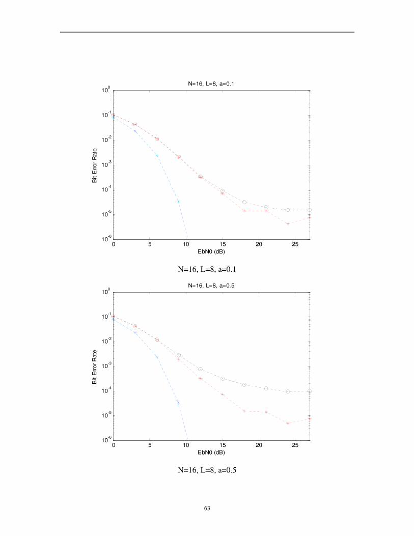
63

0 5 10 15 20 2510

-6

10-5

10-4

10-3

10-2

10-1

100

EbN0 (dB)

Bit E

rror

Rate

N=16, L=8, a=0.1

N=16, L=8, a=0.1

0 5 10 15 20 2510

-6

10-5

10-4

10-3

10-2

10-1

100

EbN0 (dB)

Bit E

rror

Rate

N=16, L=8, a=0.5

N=16, L=8, a=0.5

64

0 5 10 15 20 2510

-6

10-5

10-4

10-3

10-2

10-1

100

EbN0 (dB)

Bit E

rror

Rate

N=16,L=8,a=0.9

N=16, L=8, a=0.9

0 5 10 15 20 2510

-6

10-5

10-4

10-3

10-2

10-1

100

EbN0 (dB)

Bit E

rror

Rate

N=32, L=4, a=0.1

N=32, L=4, a=0.1

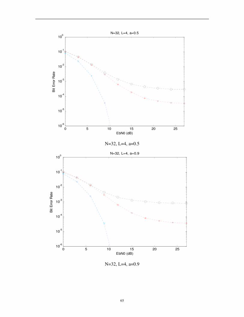
65

0 5 10 15 20 2510

-6

10-5

10-4

10-3

10-2

10-1

100

EbN0 (dB)

Bit E

rror

Rate

N=32, L=4, a=0.5

N=32, L=4, a=0.5

0 5 10 15 20 2510

-6

10-5

10-4

10-3

10-2

10-1

100

EbN0 (dB)

Bit E

rror

Rate

N=32, L=4, a=0.9

N=32, L=4, a=0.9

66

0 5 10 15 20 2510

-6

10-5

10-4

10-3

10-2

10-1

100

EbN0 (dB)

Bit E

rror R

ate

N=32, L=8, a=0.1

N=32, L=8, a=0.1

0 5 10 15 20 2510

-6

10-5

10-4

10-3

10-2

10-1

100

EbN0 (dB)

Bit E

rror

Rate

N=32, L=8, a=0.5

L=32, L=8, a=0.5

67

0 5 10 15 20 2510

-6

10-5

10-4

10-3

10-2

10-1

100

EbN0 (dB)

Bit E

rror

Rate

N=32,L=8,a=0.9

N=32, L=8, a=0.9

0 5 10 15 20 2510

-6

10-5

10-4

10-3

10-2

10-1

100

EbN0 (dB)

Bit E

rror

Rate

N=64, L=4, a=0.1

N=64, L=4, a=0.1

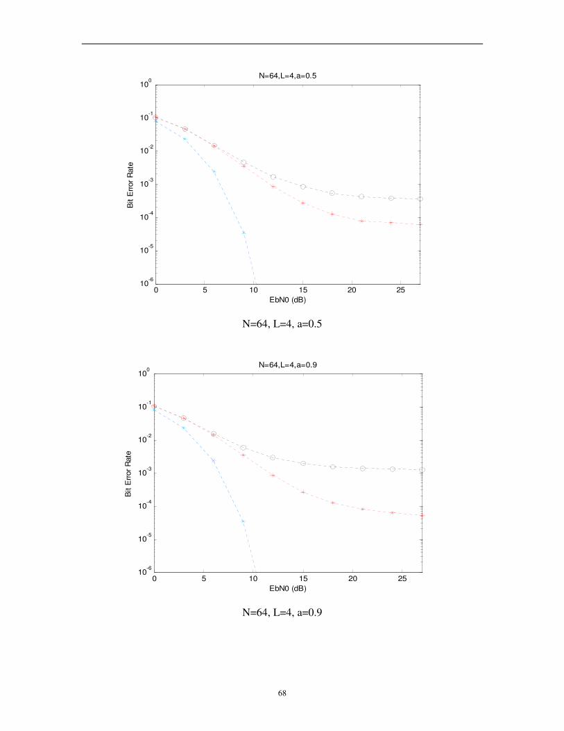
68

0 5 10 15 20 2510

-6

10-5

10-4

10-3

10-2

10-1

100

EbN0 (dB)

Bit E

rror

Rate

N=64,L=4,a=0.5

N=64, L=4, a=0.5

0 5 10 15 20 2510

-6

10-5

10-4

10-3

10-2

10-1

100

EbN0 (dB)

Bit E

rror

Rate

N=64,L=4,a=0.9

N=64, L=4, a=0.9

69

0 5 10 15 20 2510

-6

10-5

10-4

10-3

10-2

10-1

100

EbN0 (dB)

Bit E

rror

Rate

N=128, L=4, a=0.1

L=128, L=4, a=0.1

0 5 10 15 20 2510

-6

10-5

10-4

10-3

10-2

10-1

100

EbN0 (dB)

Bit E

rror

Rate

N=128, L=4, a=0.5

L=128, L=4, a=0.5

70

0 5 10 15 20 2510

-6

10-5

10-4

10-3

10-2

10-1

100

EbN0 (dB)

Bit E

rror

Rate

N=128,L=4,a=0.9

N=128, L=4, a=0.9

6.2 BER performance on the effect of timing jitters in multi-path Rayleigh

fading channel

The results of the BER performance on the effect of timing jitter in multi-path Rayleigh

fading channel are shown in this section. The dashed curve with x-mark is the results of

the BER performance from testing method one. The dashed curve with star presents the

results of the BER performance from testing method two. The dashed curve with plus

denotes the results of the BER performance from testing method three. The dashed curve

with circle shows the results of the BER performance from testing method four. The

dashdot curve gives the results of the BER performance from testing method five and the

solid curve is the ideal BER performance without interference.

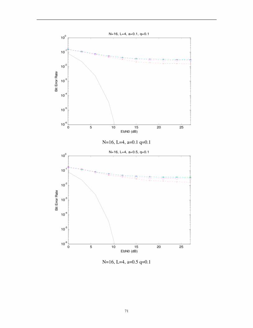
71

0 5 10 15 20 2510

-6

10-5

10-4

10-3

10-2

10-1

100

EbN0 (dB)

Bit E

rror R

ate

N=16, L=4, a=0.1, q=0.1

N=16, L=4, a=0.1 q=0.1

0 5 10 15 20 2510

-6

10-5

10-4

10-3

10-2

10-1

100

EbN0 (dB)

Bit E

rror R

ate

N=16, L=4, a=0.5, q=0.1

N=16, L=4, a=0.5 q=0.1

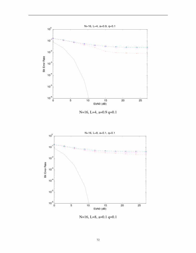
72

0 5 10 15 20 2510

-6

10-5

10-4

10-3

10-2

10-1

100

EbN0 (dB)

Bit E

rror

Rate

N=16, L=4, a=0.9, q=0.1

N=16, L=4, a=0.9 q=0.1

0 5 10 15 20 2510

-6

10-5

10-4

10-3

10-2

10-1

100

EbN0 (dB)

Bit E

rror

Rate

N=16, L=8, a=0.1, q=0.1

N=16, L=8, a=0.1 q=0.1

73

0 5 10 15 20 2510

-6

10-5

10-4

10-3

10-2

10-1

100

EbN0 (dB)

Bit E

rror

Rate

N=16, L=8, a=0.5, q=0.1

N=16, L=8, a=0.5 q=0.1

74

7. Conclusion

In this thesis, the BER performance of MC-DS-CDMA system under the effects of timing

jitters has been analyzed in the presence of AWGN channel and multi-path Rayleigh

fading channel. It can be observed from the results in Sections 6.1 & 6.2 that in general

Gaussian approximations give pessimistic BER estimates. Furthermore, the higher the

correlation between timing jitters, the less the impact on BER. The number of

sub-carriers does not appear to affect the BER significantly. The role of spreading

factor in BER performance with timing jitters needs further study.

75

Reference

1. Je-hong Jong, Performance Analysis of Coded Multicarrier Spread-Spectrum Systems

in the Presence of Multipath Fading and Nonlinearities, IEEE Communication

Magazine, Volume 49, pp. 168-179, January 2001.

2. Li-Chun Wang, and Chih-Wen Chang, On the performance of multicarrier DS-CDMA

with imperfect power control and variable spreading factors, IEEE Communication

Magazine, Volume 24, pp. 1154–1166, June 2006.

3. T. J. Lim, S.Edwards, and Sr. Rogers, An introduction to multicarrier modulation:

notes for ECE1520 Data Communications, Department of electrical and computer

engineering University of Toronto, pp.1-16.

4. — —, OFDM Tutorial, WAVE Report, 4th Wave Inc., 2007.

5. D. Matiæ, OFDM as a possible modulation technique for multimedia applications in

the range of mm waves, Introduction to OFDM, second edition, TUD-TVS, pp.1-18,

October 1998.

6. R. W. Chang, Synthesis of band-limited orthogonal signals for multichannel data

transmission, The Bell Systems Technical Journal, Volume 45, pp. 1775-1796,

December 1966.

7. B. R. Saltzberg, Performance of an efficient parallel data transmission system, IEEE

Transactions on Communication Technology, Volume COM-15, December 1967.

8. R. R. Mosier, and R. G. Clabaugh, Kineplex, a bandwidthefficient binary transmission

system, AIEE Transactions, Volume 76, pp. 723- 728, January 1958.

9. — —, Orthogonal frequency division multiplexing, U.S. Patent 3,488,445, filed

November 14, 1966, issued January 6, 1970.

76

10. W. Y. Zou, and Y.Wu, COF'DM: an overview, IEEE Transactions on Broadcasting,

Volume 41, No. I, March 1995.

11. S. B. Weinstein, and P. M. Ebert, Data transmission by frequency division

multiplexing using the discrete Fourier transform, IEEE Transactions on

Communication Technology, Volume COM-19, No. 15, October 1971.

12. E. Bidet, C. Joanblanq, and P. Senn, A fast 8K FFT VLSI chip for large OFDM single

frequency networks, Proceedings of the International Conference on HDTV 94,

Torino, Italy, October 1994.

13. R. V. Nee, and R. Prasad, OFDM for Wireless Multimedia Communications, Artech

House, Boston, London, 2000.

14. G. C. Porter, Error distribution and diversity performance of a frequency-differential

PSK HF modem, IEEE Transactions on Communication Technology, Volume

COM-16, pp. 567-575, August 1968.

15. M. S. Zimmerman, and A. L. Kirsch, The AN/GSC-10 (KATHRYN) variable rate data

modem for HF radio, IEEE Transactions on Communication Technology, Volume

COM-15, pp. 197-205, April 1967.

16. P. A. Bello, Selective fading limitations of the Kathryn modem and some system

design considerations, IEEE Transactions on Communication Technology, Volume

COM-13, pp. 320-333, September 1965.

17. B. Hirosaki, An orthogonally multiplexed QAM system using the discrete Fourier

transform, IEEE Transactions on Communications, Volume COM-29, pp. 982-989,

July 1981.

77

18. B. Hirosaki, A 19.2 kbits voiceband data modem based on orthogonally multiplexed

QAM techniques, Proceedings of IEEE International Conference on Communications,

pp.21.1.1-5, 1985.

19. W. E. Keasler, and D. L. Bitzer, High speed modem suitable for operating with a

switched network, U.S. patent No. 4,206,320, June 1980.

20. E. F. Casas, and C. Leung, OFDM for data communication over mobile radio FM

channels-part 1: analysis and experimental results, IEEE Transactions on

Communications, Volume. COM-39, No.5, May 1991.

21. P. S. Chow, J. C. Tu, and J. M. Cioffi, Performance evaluation of a multichannel

transceiver system for ADSL and VHDSL services, IEEE Journal on Selected Area in

Communications, Volume SAC-9, No.6, pp.900-919, August 1991.

22. P. S. Chow, J. C. Tu, and J. M. Cioffi, A discrete Multitone transceiver system for

HDSL applications, IEEE Journal on Selected Area in Communications, Volume

SAC-9, No. 6, pp.909-919, August 1991.

23. B. Sueur, D. Castelain, G. Degoulet, M. Riviere, and B. LeFloch, Digital Terrestrial

Broadcasting of Audiovisual Signals, Spectrum 20120 conference, Toronto,

September 1992.

24. B. LeFloch, M. Alard, and C. Berrou, Coded Orthogonal Frequency Division

Multiplex, Proceedings of the IEEE, Volume 83, No. 6, June 1995.

25. Q. Wang, and L. Y. Onotera, Coded QAM Using a Binary Convolutional Code, IEEE

Transactions on Communications, Volume 43, No.6, June 1995.

26. — —, an introduction to direct-sequence spread-spectrum, application note 1890,

Maxim Integrated Products, Feb 2003.

78

27. — —, Spread Spectrum Systems, chapter 8 module 7: Wireless Communications,

ICT Technologies, pp.74-87.

28. K. Feher, Wireless Digital Communications: Modulation and Spread Spectrum

Applicaions, Prentice Hall PTR, Prentice-Hall, Inc., 1995.

29. L.Hanzo, L-L. Yang, E-L.Kuan, and K. Yen, single-and multi-carrier CDMA:

multi-user detection, space-time spreading, synchronization, networking, and

standards, IEEE press, IEEE communications society, 2003.

30. S. Hara, and R. Prasad, Overview of Multicarrier CDMA, IEEE Communication

Magazine, Volume 35, pp. 126–133, December 1997.

31. E. Sourour, and M. Nakagawa, Performance of Orthogonal Multicarrier CDMA in a

Multipath Fading Channel, IEEE Transactions on Communications, Volume 44, No.

3, pp. 356-67, March 1996.

32. M. K. Simon, and M. S. Alouini, BER Performance of multicarrier DS-CDMA

systems over generalized fading channels, IEEEE communication theory

mini-conference, pp.72-77, June1999.

33. J. Hou, and M. H. Lee, Dual OVSF Codes with Lower Correlations, IEICE

Transactions on Fundamentals of Electronics, Communications and Computer

Sciences, Volume E89-A, Issue 11, pp. 3363-3367, November 2006.

34. M. H. Lee, A new reverse jacket transform and its fast algorithm, IEEE Transactions

on Circuits and Systems II, Volume 47, No. 1, pp. 39-47, January 2000.

35. W. U. Bajwa, A. Sayeed, and R. Nowak, Sparse Multipath Channels: Modeling and

Estimation, 13th IEEE Digital Signal Processing Workshop and 5th IEEE Signal

79

Processing Education Workshop, pp. 320-325, January 2009.

36. A. C. Brooks, and S. J. Hoelzer, Design and Simulation of Orthogonal Frequency

Division Multiplexing (OFDM) Signaling: Final Report, Electrical and Computer

Engineering Department, Bradley University, pp. 1-50, May 2001.

37. K. V. S. Hari, et. al., Channel Models for Fix Wireless Applications, IEEE 802.16

Broadband Wireless Access Working Group, pp. 1-36, July 2001.

38. H. Steendam and M. Moeneclaey, Sensitivity of orthogonal frequency division

multiplexed systems to carrier and clock synchronization errors, Signal Processing,

Volume 80, pp. 1217-1229, July 2000.

39. H. Steendam, The Effect of Timing Jitter on MC-DS-CDMA, IEEE Transactions

Communications, Volume 52, No. 3, pp. 467-472, March 2004.

40. U. Onunkwo, Y. Li, and A. Swami, Effect of Timing Jitter on OFDM-Based UWB

Systems, IEEE Journal on Selected Areas in Communications, Volume 24, No. 4, pp.

787-793, April 2006.

41. L. Tomba, and W. A. Krzymien, A model for the analysis of timing jitter In OFDM

systems, Proceedings of IEEE International Conference on Communications, Volume

3, pp. 1227-1231, June 1998.

42. L. Tomba, and W. A. Krzymien, An analysis of the effect of chip timing jitter in

MC-CDMA systems, IEEE Transactions on Vehicular Technology, Volume 48, No. 6,

pp. 1889-1898, November 1999.

43. T. L. Carroll, and L. M. Pecora, synchronization in chaotic systems, Physical

Review letters, 64(8), pp. 821-825, February 1990.

80

44. K. Black, Matlab Tutorial, Department of Mathematics, Clarkson University.

45. T. Pollet, P. Spruyt, and M. Moeneclaey, the BER Performance of OFDM systems

using non-synchronized sampling, Globecom 1994, San Fransisco CA, Paper S7.6,

pp. 253-257, November 1994.

46. M. Moeneclaey, the effect of synchronization errors on the performance of

orthogonal frequency-division multiplexed (OFDM) systems, Proc. COST 254,

Emerging techniques for communication terminals, Toulouse, France, pp.41-45, July

1997.

47. H. Steendam, and M. Moeneclaey, the effect of carrier frequency offsets on downlink

and uplink MC-DS-CDMA, IEEE Journal on Selected Area in Communications,

Volume 19, No. 12, pp. 2528-2536, December 2001.

81

Appendix: Complete Matlab codes

A1 OVSF code:

function [L,Code,R,C] = ovsf(L,index)

clc

if index==1

j4=[1,1,1,1;1,-i,i,-1;1,i,-i,-1;1,-1,-1,1];

I=eye(4);

pr=I([1,4,3,2],:);

pc=I([2,3,4,1],:);

mj4=pr*j4*pc;

cj4=mj4;

cj2=cj4;

if L>4

temp=cj2;

for k=1:L/8

clear cj1;

for l=1:2^(k+1);

cj1=temp(l,:);

cjt(2*l-1:2*l,:)=[cj1 cj1;cj1 -cj1];

clear cj1

end

temp=cjt;

clear cjt;

end

clear cj2;

cj2=temp;

end

Code=cj2;

for m=1:L;

cj=cj2(m,:);

for t=1:L;

a= circshift(cj,[0 1-t]);

r=cj.*conj(a);

x=sum(r);

y(t)=x;

end

R(m,:)=y;

end

82

for m=1:L-1;

cj2a=cj2(m,:);

for n=(m+1):L;

cj2b=cj2(n,:);

for t=1:L;

b= circshift(cj2b,[0 1-t]);

r=cj2a.*conj(b);

x=sum(r);

c(t)=x;

end

T(n,:)=c;

end

C(:,:,m)=T;

end

end

if index==2

H=hadamard(L);

for l=1:L;

W(l,:)=H(l,:);

end

Code=W;

for m=1:L;

w=W(m,:);

for t=1:8;

a= circshift(w,[0 t-1]);

r=w.*conj(a);

x=sum(r);

y(t)=x;

end

R(m,:)=y;

end

for m=1:L-1

wa=W(m,:);

for n=(m+1):L

wb=W(n,:);

for t=1:8;

b= circshift(wb,[0 1-t]);

r=wa.*conj(b);

x=sum(r);

c(t)=x;

end

T(n,:)=c;

83

end

C(:,:,m)=T;

end

end

A2 Simulation code of the MC-DS-CDMA system in AWGN channel:

close all;

clear

clc

usernumber=1;

[L,code,R,C] = ovsf(4,2);

W=[];

Ts=(1/528)*10^(-6);

N=16;;

Nsample=N*1;

a=0.5;

q=0.1*Ts;

nn=0:(L*Nsample-1);

auto=a.âbs(nn);

cv=toeplitz(auto);

ch=chol(cv);

ref_W=[];

ref_w=code(usernumber,:);

for l=1:L;

ref_signal_w=repmat(ref_w(l), [1,(Nsample+Nsample/4)]);

ref_W=[ref_W,ref_signal_w];

end

84

Num_total=1*10^2;

for Num=1:Num_total;

display (Num);

ran=randn(1,Nsample*L);

erro_m=ran*ch;

erro_r=randn(1,Nsample*L)*q/Ts;%white sampling jitter

erro_c=erro_m*q/Ts;%correlated sampling jitter

erro_i=zeros(1,Nsample*L);%no sampling jitter

erro=[erro_r;erro_c;erro_i];

for u=1:L

input=rand(1,N-4)>=0.5;

inputcode(u,:)=input;

mo = input*(-2)+1;

mo_f=zeros(1,N);

%mo_4=circshift(mo_3,[0 3]);

%mo_f=[mo_2,mo_4];

mo_f(:,2:((N-4)/2+1))=mo(:,1:(N-4)/2);

mo_f(:,(N-(N-4)/2+1):N)=mo(:,((N-4)/2+1):(N-4));

for tt=1:3

for n_symbol=1:L

index=(n_symbol-1)*Nsample;

if tt~=3,

for n=1:Nsample

85

for k=1:N

d(k)=mo_f(k)*exp(j*2*pi*(k-1)*((n-1)+erro(tt,index+n))/Nsample);

end

iff_sig(n)=sum(d);

end

else

iff_sig= ifft(mo_f)*Nsample;%Inverse discrete Fourier transform%

end

ad=iff_sig(:,(Nsample-Nsample/4+1):Nsample);%get guard interval%

sign=[ad,iff_sig];%insert the guard interval%

index_lg=(n_symbol-1)*(Nsample+Nsample/4)+1;

index_rg=n_symbol*(Nsample+Nsample/4);

signal(1,index_lg:index_rg)=sign;

end

w=code(u,:);

for l=1:L;

signal_w=repmat(w(l), [1,(Nsample+Nsample/4)]);

W=[W,signal_w];

end

out2=signal.*W;

user(u,:,tt)=out2;

W=[];

end

end

86

user_m=sum(user,1);

[m1,m2,m3]=size(user_m);

Ksnr=0;

DIFF=10*log10(N*L/(N-4));

for SNR=0-DIFF:3:27-DIFF

Ksnr=Ksnr+1;

EbN0(Ksnr)=SNR+DIFF;

Pawgn=(N-4)/10^((SNR)/10);

awgnx=randn(m2,1).*sqrt(Pawgn/2);

awgny=randn(m2,1).*sqrt(Pawgn/2);

Noise=complex(awgnx,awgny);

for tt=1:3;

user_mm=user_m(:,:,tt);

user_f=user_mm.';

awgn_sig=user_f+Noise;

s=awgn_sig.*conj(ref_W.');

y0=reshape(s,(Nsample+Nsample/4),L);

y1=permute(y0,[2 1]);

y2=sum(y1); %returns sums along the same columns of an array%

y3=y2/L;

y4=y3(:,(Nsample/4+1):(Nsample+Nsample/4));

fft_sig=fft(y4);%Discrete Fourier transform%

del_1=fft_sig(:,2:((N-4)/2+1));

del_2=fft_sig(:,(N-(N-4)/2+1):N);

87

del_sig=[del_1,del_2];%remove the inefficient bits from data stream%

out=1-(real(del_sig)>=0);%pskdemod(del_sig,2);%bpsk demodulation%

if Num==1

n_error(tt,Ksnr)=0;

end

n_error(tt,Ksnr)=n_error(tt,Ksnr)+sum(xor(inputcode(usernumber,:),out));

end

end

end

BER_r=n_error(1,:)/((N-4)*Num_total);

BER_c=n_error(2,:)/((N-4)*Num_total);

BER_i=n_error(3,:)/((N-4)*Num_total);

BER=0.5*erfc(sqrt(10.^(EbN0/10)));

semilogy(EbN0,BER,'bx:',EbN0,BER_r,'r*:',EbN0,BER_c,'ko:',EbN0,BER_i,'c+:');

axis([0 27 10^(-6) 10^(0)]);

xlabel('EbN0 (dB)');

ylabel('Bit Error Rate');

title(['N=',num2str(N),', L=',num2str(L),', a=',num2str(a), ]);

A3 Simulation code of the MC-DS-CDMA system in multi-path

Rayleigh fading channel:

close all;

clear

clc

[L,code,R,C] = ovsf(4,1);

88

Nuser=L;%total number of users

usernumber=1;

Ts=(1/528)*10^(-6);

N=16;%16;

Nsample=N*1;

a=0.9;

% q=0.1*Ts;

q=0.1;

Qs=1;

nnn=0:(L*Nsample-1);

auto=a.âbs(nnn);

cv=toeplitz(auto);

ch=chol(cv);

Num_total=100;

data=zeros(Num_total,N);

datacoded=zeros(Num_total,N);

Gi=zeros(Num_total,N);

Ai=zeros(Num_total,N);

Bi=zeros(Num_total,N);

Ui=zeros(Num_total,N);

M=4;

G=sum(exp(-0.69*(0:M-1)));

KK=Num_total;

h1=complex(randn(M,KK),randn(M,KK)).*repmat(sqrt(exp(-0.69*(0:M-1)')),1,KK)/sqrt(

2)/sqrt(G);

tmp=fft(h1,Nsample);

89

tmpp=permute(tmp,[2 1]);

Noise=complex(randn(Num_total,Nsample*L), randn(Num_total,Nsample*L));

Ni=zeros(Num_total,N);

for Num=1:Num_total;

display (Num);

ran=randn(1,Nsample*L);

erro_m=ran*ch;

erro_c=erro_m*q;

erro=reshape(erro_c,N,L);

erro=permute(erro,[2 1]);

Noise_t1=Noise(Num,:);

Noise_t2=reshape(Noise_t1,N,L);

Noise_t3=permute(Noise_t2,[2 1]);

input=zeros(L,N);

inputcode=zeros(L,N);

for u=1:L;

in=rand(1,N)>=0.5;

mo = in*(-2)+1;%pskmod(input,2);

input(u,:)=in;

inputcode(u,:)=mo;

end

data(Num,:)=input(usernumber,:);

datacoded(Num,:)=inputcode(usernumber,:);

90

for i=0:N-1;

temp=0;

for m=1:L;

for n=0:N-1;

temp=temp+exp(j*2*pi*i*erro(m,n+1)/N)*tmpp(Num,i+1);

end

end

Gii(Num,i+1)=temp/N;

end

for i=0:N-1;

temp=0;

for k=0:N-1;

if k==i;

continue;

else

for m=1:L;

for n=0:N-1;

temp=temp+inputcode(usernumber,k+1)*exp(j*2*pi*((k-i)*n+k*erro(m,n+1))/N)*tmpp(

Num,k+1);

end

end

end

end

Aii(Num,i+1)=temp/N;

end

for i=0:N-1;

temp=0;

91

for k=0:N-1;

if k==i;

continue;

else

for l=1:Nuser;

if l==usernumber;

continue;

else

for m=1:L;

for n=0:N-1;

temp=temp+inputcode(l,k+1)*code(l,m)*conj(code(usernumber,m))*exp(j*2*pi*((k-i)*n

+k*erro(m,n+1))/N)*tmpp(Num,k+1);

end

end

end

end

end

end

Bii(Num,i+1)=temp/N;

end

%=========================================================%

%==============================================================

========%

for i=0:N-1;

temp=0;

for l=1:Nuser;

if l==usernumber;

92

continue;

else

for m=1:L;

for n=0:N-1;

temp=temp+inputcode(l,i+1)*code(l,m)*conj(code(usernumber,m))*exp(j*2*pi*i*erro(m

,n+1)/N)*tmpp(Num,i+1);

end

end

end

end

Uii(Num,i+1)=temp/N;

end

for i=0:N-1;

temp=0;

for m=1:L;

for n=0:N-1;

temp=temp+conj(code(usernumber,m))*Noise_t3(m,n+1)*exp(j*2*pi*i*n/N)*conj(tmpp

(Num,i+1));

end

end

Nii(Num,i+1)=temp/N;

end

end

Gi=Gii;

Ai=Aii;

Bi=Bii;

Ui=Uii;

Ni=Nii;

93

%=====calculate variance of Ai, Bi, Ui for Method 4=======%

Var_Ai=zeros(1,N);

Var_Bi=zeros(1,N);

Var_Ui=zeros(1,N);

for i=0:N-1,

temp=0;

for k=0:N-1

if k==i

continue

else

for m=1:L

for mm=1:L

for n=0:N-1

for nn=0:N-1

d=abs((m-mm)*N+n-nn);

temp=temp+exp(-4*pi^2/N^2*k^2*q^2*(1-a^d))*exp(j*2*pi/N*(k-i)*(n-nn));

end

end

end

end

end

end

Var_Ai(i+1)=Var_Ai(i+1)+real(temp)/N^2;

temp=0;

for l=1:Nuser

if l==usernumber

continue

else

94

for k=0:N-1

if k==i

continue

else

for m=1:L

for mm=1:L

temp1=0;

for n=0:N-1

for nn=0:N-1

d=abs((m-mm)*N+(n-nn));

temp1=temp1+exp(-4*pi^2/N^2*k^2*q^2*(1-a^d))*exp(j*2*pi/N*(k-i)*(n-nn));

end

end

temp=temp+temp1*code(l,m)*code(l,mm)*conj(code(usernumber,m))*conj(code(usernu

mber,mm));

end

end

end

end

end

end

Var_Bi(i+1)=Var_Bi(i+1)+real(temp)/N^2;

temp=0;

for l=1:Nuser

if l==usernumber

continue

else

for m=1:L

95

for mm=1:L

temp1=0;

for n=0:N-1

for nn=0:N-1

d=abs((m-mm)*N+(n-nn));

temp1=temp1+exp(-4*pi^2/N^2*i^2*q^2*(1-a^d));

end

end

temp=temp+temp1*code(l,m)*code(l,mm)*conj(code(usernumber,m))*conj(code(usernu

mber,mm));

end

end

end

end

Var_Ui(i+1)=Var_Ui(i+1)+temp/N^2;

end

%====================================%

%==calculate variance of Ai, Bi, Ui for Method 5==================%

%==========================================%

for i=0:N-1;

%DD2=0;

for k=0:N-1;

d21=0;

d22=0;

d23=0;

d24=0;

96

if k==i;

continue;

else

for m=1:L

for mm=1:L

for n=0:N-1;

for nn=0:N-1

d1=(m-mm);

d2=(n-nn);

if m==mm && n==nn;

d21=d21+L*Qs^2;

% D21=[D21,d21];

elseif m==mm && n~=nn

%nnn=n-nn;

d22=d22+L*(Qs^2/N^2)*(N-abs(d2))*cos(2*pi*(k-i)*abs(d2)/N)*exp(-4*pi^2*k^2*q^2

*(1-aâbs(d2))/N^2);

elseif m~=mm && n==nn;

%mmm=m-mm;

d23=d23+(Qs^2/N)*(L-abs(d1))*exp(-4*pi^2*k^2*q^2*(1-aâbs(d1*N))/N^2);

elseif m~=mm && n~=nn;

d24=d24+(Qs^2/N^2)*(N-abs(d2))*(L-abs(d1))*cos(2*pi*(k-i)*abs(d2)/N)*exp(-4*pi^2

*k^2*q^2*(1-aâbs(N*d1+d2))/N^2);

end

DD2=(d21+d22+d23+d24);

end

end

97

%DD2=d21+d22+d23+d24;

end

end

end

end

Di2(i+1)=DD2/(N^2);

for l=1:Nuser

if l==usernumber

continue

else

for k=0:N-1;

if k==i;

continue;

else

for m=1:L;

for mm=1:L

d31=0;

d32=0;

d33=0;

d34=0;

for n=0:N-1;

for nn=0:N-1

d1=(m-mm);

d2=(n-nn);

if m==mm && n==nn;

d31=d31+L*Qs^2*Nuser;


d32=d32+L*(Qs^2/N^2)*(N-abs(d2))*cos(2*pi*(k-i)*abs(d2)/N)*exp(-4*pi^2*k^2*q^2

98

*(1-aâbs(d2))/N^2);


cd=code(l,m)*code(l,mm)*conj(code(usernumber,m))*conj(code(usernumber,mm));

d33=d33+(Qs^2/N)*(L-abs(d1))*cd*exp(-4*pi^2*k^2*q^2*(1-aâbs(N*d1))/N^2);



d34=d34+(Qs^2/N^2)*(N-abs(d2))*(L-abs(d1))*cos(2*pi*(k-i)*abs(d2)/N)*cd*exp(-4*p

i^2*k^2*q^2*(1-aâbs(N*d1+d2))/N^2);

end

end

end

DD3=(d31+d32+d33+d34);

end

end

end

end

end

end

Di3(i+1)=DD3/N^2;

%=====================================================%

%============================================================%

for l=1:Nuser

if l==usernumber

continue

else

99

for m=1:L;

for mm=1:L

d41=0;

d42=0;

d43=0;

d44=0;

for n=0:N-1;

for nn=0:N-1

d1=(m-mm);

d2=(n-nn);

if m==mm && n==nn;

d41=d41+L*Qs^2*Nuser/N;


%nnn=n-nn;

d42=d42+L*(Qs^2/N^2)*(N-abs(d2))*exp(-4*pi^2*i^2*q^2*(1-aâbs(d2))/N^2);



d43=d43+(Qs^2/N)*(L-abs(d1))*cd*exp(-4*pi^2*i^2*q^2*(1-aâbs(N*d1))/N^2);


%mmm=m-mm;

%nnn=n-nn;


d44=d44+(Qs^2/N^2)*(N-abs(d2))*(L-abs(d1))*cd*exp(-4*pi^2*i^2*q^2*(1-aâbs(N*d

1+d2))/N^2);

end

end

100

end

DD4=d41+d42+d43+d44;

end

end

end

end

Di4(i+1)=DD4/(N^2);

end

%===calculate variance of Ai, Bi, Ui for Method 5==================%

Ksnr=0;

Z=zeros(Num_total,N);

DIFF=10*log10(L);

for SNR=0-DIFF:3:27-DIFF

Ksnr=Ksnr+1;

EbN0(Ksnr)=SNR+DIFF;

Pawgn=N/10^((SNR)/10);

Z=real((Gi.*datacoded+Ai+Bi+Ui).*conj(tmpp)+Ni*sqrt(Pawgn/2));

out=1-(Z>=0);%bpsk demodulation%

error_bits=xor(data,out);

BERs_M1(Ksnr,:)=sum(error_bits)/Num_total;%BER of each subcarrier

BER_M1(Ksnr)=sum(BERs_M1(Ksnr,:))/N;%overall BER

%=Method 2: Monte Carlo simulation with AWGN variance calculated from

simulation====%

Z_var2=mean(real((Ai+Bi+Ui).*conj(tmpp)+Ni*sqrt(Pawgn/2)).^2);

ber_conditional2=erfc(real(Gi.*conj(tmpp))./(repmat(real(sqrt(Z_var2*2)),Num_total,1).

*(abs(tmpp))))*0.5;

101

BERs_M2(Ksnr,:)=sum(ber_conditional2)/Num_total;%BER of each subcarrier

BER_M2(Ksnr)=sum(BERs_M2(Ksnr,:))/N;%overall BER

%=======Method 3: Monte Carlo simulation with AWGN variance calculated from

SNR setting====%

Z_var3=mean(real((Ai+Bi+Ui).*conj(tmpp)).^2)+Pawgn/2*(L/N);


*(abs(tmpp))))*0.5;

BERs_M3(Ksnr,:)=sum(ber_conditional3)/Num_total;

BER_M3(Ksnr)=sum(BERs_M3(Ksnr,:))/N;

%=======Method 4: Monte Carlo simulation with all interference variance calculated

from formula====%

Z_var4=(Var_Ai+Var_Bi+Var_Ui)/2.*var(tmpp).*var(conj(tmpp))+Pawgn/2*(L/N);


*(abs(tmpp))))*0.5;


BER_M4(Ksnr)=sum(BERs_M4(Ksnr,:))/N;

%=======Method 5: ====%

Z_var5=(Di2+Di3+Di4)/2.*var(tmpp).*var(conj(tmpp))+Pawgn/2*(L/N);


*(abs(tmpp))))*0.5;


BER_M5(Ksnr)=sum(BERs_M5(Ksnr,:))/N; end

BER=0.5*erfc(sqrt(10.^(EbN0/10)));

semilogy(EbN0,BER,'k',EbN0,BER_M1,'rx:',EbN0,BER_M2,'b*:',EbN0,BER_M3,'g+:',

EbN0,BER_M4,'mo:',EbN0,BER_M5,'c-.');

axis([0 27 10^(-6) 10^(0)]);

xlabel('EbN0 (dB)');

102

ylabel('Bit Error Rate');

title(['N=',num2str(N),', L=',num2str(L),', a=',num2str(a),', q=',num2str(q)]);

Documents

BER performance of MC-DS-CDMA systems in the presence … · BER Performance of MC-DS-CDMA Systems in the Presence of Timing Jitter . A thesis presented in partial fulfillment of