Benin Agriculture Productivity and profitability Measurementageconsearch.umn.edu/bitstream/126748/2/9682-RJA1.doc1.pdf · 5 Productivity is defined as the relationship between output

2

Benin Agriculture Productivity and profitability Measurement

Labintan Adeniyi Constant1 and Ding Shijun2

1. Dr in Agricultural Economics ,

2. Prof in Agricultural Economics

Zhongnan University of Economics and Law, Wuhan, China

182# Nanhu Avenue, East Lake High-tech Development Zone, Wuhan 430073, P.R.China

Selected Poster prepared for presentation at the International Association of Agricultural

Economists (IAAE) Triennial Conference, Foz do Iguaçu, Brazil, 18-24 August, 2012. Copyright 2012 by [authors]. All rights reserved. Readers may make verbatim copies of this document for non-commercial purposes by any means, provided that this copyright notice appears on all such copies.

3

Abstract

This paper explored the Benin agricultural productivity and profitability under occurred reform

since 1961 to 2008. Productivity and profitability has been evaluated using the new approach

developed by O’Donnell(2008).In the approach Productivity is obtain using Hick Moorsteen

index decomposition into Technical Change, mix Efficiency change and Scale Efficiency

Change while Profitability is obtain using productivity and Term of Trade product. To achieved

the purpose of this paper, agricultural output-input quantity and prices data have been collected

from FAO stat, Benin Country FAO statistical database and Benin National Agricultural Institute

Database during the period 1961-2008. All data are computing using the DPIN software

developed by O’Donnell (2010).

It is found that since the country national independency in 1961, Benin agriculture productivity

has decreased. The decreased has been more significant after the sector liberalization while the

term of trade has been much improved and profitability increased. This situation explains that

after the liberalization, competiveness has decreased and monopolization increased. It can be

conclude that most private stakeholder involve in the sector during post liberalization has earn

more profit than invest to contribute at the sector productivity growth.

The paper indentify that the country doesn’t improved agricultural productivity after the sector

liberalization in opposite to the normal figure that liberalization will stimulate technology

transfer and development which will improve productivity. The situation will then highlight

policies maker to identify news strategy which can help to optimize the production and

agriculture resources efficiency.

Key -words: Agricultural-Productivity- Profitability-Benin-Reform

Introduction

Like most Sub-Sahara economies, in Benin agricultural is a dominant sector for economic

growth, food security and to poverty alleviation. Its contributes more than 20% of country’s

Gross Domestic Product Growth (GDP ), and employs at least 60% of country’s population

(BAfD/OCDE, 2008) mostly women’s who have access to small pieces of land (1.7 ha per 7

4

peoples) provides 90% of export earnings and participates in 15% of state revenue

(MAEP-MDEF1,2006). Over decades, the country’s agricultural growth was on downward trend.

However, comparing to developed countries agriculture growth which have been increased

highly substantially over several decade, Benin agriculture growth has decreased. This situation

generates polarized debate regarding the real impact of agricultural sector growth decreased on

the country poverty alleviation goals.

Moreover, Benin’s has undergone several reforms under different political regimes since

1961.However the important reform started from 1990 with the Country openness economy and

agriculture liberalization in purpose to stimulate the country economic growth. There is evidence

that agricultural as key sector for the country economic growth, will certainly been affected.

The productivity question in Benin is not new topic but very little empirical study has been done

in this field to evaluate the whole country agricultural productivity. Most study are sectorial

studies focused only in cotton productivity (MAEP,2010;MFE2,2010; Sekloka, et al , 2009;

Nicolas.P,2011) or cassava productivity(Adekambi et al, 2010; ESC3, 2004)

This paper aims to explore the Benin’s agricultural productivity and profitability from 1961 to

2008 and evaluate the variation over that period.

The first section outlines the concepts of productivity and profitability and reviews various

frameworks which assist in evaluating both factors and identified the best approach. The second

section will be applied the best approach to evaluate agricultural productivity and profitability in

Benin and analysis each factor variation. The last part will be for conclusion and policies.

1-Productivity and Profitability Measurement

1 MAEP-MDEF :Ministry of Agricultural, Livestock and Fishery- Ministry of Development, Economic and Finance 2 Ministry of Economics and Finance

3 Equipe Sectoriel Des Contrepartis

5

Productivity is defined as the relationship between output generated by production and service

and the input provided to produce this output (Joseph Prokopenko, 1987). According to the same

author, productivity means resources (labor, capital, material, energy and information change)

efficient use.

Chambers (1988) argued that productivity measurement is an approach to measure the

production rate of technical change and can be conceptualized as comprising two main

components. The first component is partial factor productivity (PFP) and expressed as the ratio

of total output Y and any xi input used to produce that output. The second component is the total

output Y ratio with summation of all input Xi

However, it is very complex most of time to quantify the exact input used to produce a certain

amount of output. When the input is visible, it is in form of good and invisible when it is in form

of service (Gboyega, 2000). From this point of view, it seems that various components are

involved in output production and this makes more complex the exact description of input

components. To overcome this complexity, a common approach is to consider labour (human

resources), capital (physical and financial assets), and material as input components with time

becoming the denominator of output with the assumption that capital, energy and other factors

are regarded as aids to individual productivity.

(a) Furthermore, there are several methods to aggregate inputs and outputs for productivity

measurement. Grosskopf (1993) conclude that there are four productivity measurement

methods which could be base on frontier output or on non frontier output: (a) Econometric

production models; (b) total factor productivity indices; (c) data envelope analysis (DEA);

and (d) stochastic frontiers (Coelli,Rao and Battese, 1998).

6

Figure1: Summarized of Previous Productivity Measurement Methods

Sources: Grosskopf (1993)

The econometric methods are based on the determination of the production function or dual /cost

profit function. The important benefit of this approach is that its econometric implementation

yields parameter estimates of the production technology in the process of measuring productivity

advancement. But it request to know the production function (ex: the Cob-Douglas production

function) base on Solow growth model.

Nonetheless, the Malmquist index base on Caves, Christensen, and Diewert (1982) research and

using the distance function are very good tools to measure and analyse productivity. Indeed Färe

et al. (1994) proposed use of the distance function approach first proposed by Shepherd (1970)

and Fare(1988) to calculate the Malmquist TFP as geometric mean of output Malmquist index

and input Malmquist index. They found that the TFP can be decomposed as a product of two

-Growth Accounting Equation

-Divisia Index

-Exact Index

-Tornquist Index

Non-Frontier Approach

Frontier Approach

Non-Parametric Index Approach Number

Parametric Non-Parametric Parametric

-Programming

-Econometric Approach

-Malmquist Productivity Index

-Stochastic and deterministic Model

Econometric Model

7

forms of efficiency factors which are technical change and technical efficiency change. Fare et al

(1994) utilize the Data Envelopment Analysis (DEA) approach. This is a nonparametric

approach based on linear programming to compute these two efficiency factors. The

nonparametric Malmquist index became very popular as it is easy to compute. Furthermore, the

approach does not require information on cost or revenue shares to aggregate inputs or outputs,

consequently, it less demanding in terms of data. Furthermore, The approach allows into changes

in efficiency and technology to be broken down (Shih et al, 2003; Alejandro and Bingxin, 2008).

In addition, the method does not attract any of the stochastic assumption restrictions. Despite

this, it is susceptible to the effects of data noise, and can suffer from the problem of ‘unusual’

shadow prices, when degrees of freedom are restricted (O'Donnell, Coelli and Timothy, 2005).

The issue of shadow prices is important and is one that is not well understood among authors

who apply the Malmquist DEA methods. By contrast, DEA methods in measuring productivity

growth which differ from pure index approach such as Fisher and Tornkvist indexes do not

require any price data. The concept is more evident in agriculture where input price data are

seldom available and could at any times be distorted by the government policies.

The productivity evaluation Malmquist TFP approach based on DEA method has been applied

by several scholars to evaluate several countries, regions and provinces in terms of both overall

productivity and in various individual sectors over the past decades (Fare et al , 1994; David and

Elliot ,1998 ; Shih-Hsun et al , 2003; Vu , 2003; Tim and Shannon , 2005 ; Carlos ,2010).

Indeed, Fare et al (1994) has applied the method to analysis productivity growth in 17 OECD

countries over the period 1979-1988.They found that US productivity growth is slightly higher

than an average country in the OECD region and it was due to technical change in the US

agriculture sector while Japan’s productivity growth is highest with almost half due to efficiency

change.

Michael A. Trueblood used the method to evaluate intercountry agricultural productivity growth

over the period of 1961-1991. It was the most comprehensive sample of countries in the world to

date. The study found that globally, productivity declined during the 1960s and 1970s, but

rebounded in the 1980s. Developing economies’ productivity declined over 1961-1991 while

8

developed economies exhibited positive production growth, demonstrating a widening

productivity gap. North America and Western Europe registered high growth while Asia and

Sub-Sahara Africa registered negative growth. Differences were attributed toward policies of

greater economic openness and the effectiveness of the ‘Green revolution’.

Carlos(2010) used the method to evaluate Latin America and Caribbean agricultural productivity

in comparison to the rest of the world during the period 1961-2007. It was found that among

developing regions, Latin America and the Caribbean had the highest agricultural productivity

growth during the last two decades, due particularly to improvements in efficiency and the

introduction of new technologies. This has been achieved through strong land allocation and

agriculture policies. This was the case in Brazil and Cuba which policies that do not discriminate

against agricultural sectors and that remove price and production distortions were considered to

have helped improve productivity growth.

David and Elliott (1998) have also applied the Malmquist DEA method to evaluate change in

Chinese provincial agriculture productivity after the China’s agricultural reform opening. They

found significant variation in productivity change from year-to-year and from

province-to-province. They concluded that de-collectivization in the early 1980s accounted for a

significant expansion of agricultural productivity, while rural industrialization registered the

opposite effect. In addition, they found that productivity was also sensitive relative grain prices,

to natural disasters including flood and drought, and the proximity of a given province to coastal

areas.

Shih-Hsun Hsu et al (2003) has also applied the Malmquist productivity indexes and it

decomposition using DEA approach to evaluate China’s 27 provinces agricultural productivity to

analyze then the productivity growth in China’s agricultural sector over the period1984-1999 .He

found that over all the considered period TFP growth remains sluggish in China’s agricultural

Similarly, Vu (2003) applies Malmquist productivity index method to measure total factor

productivity (TFP) growth in Vietnamese agriculture using panel data from 60 provinces in

Vietnam over the period 1985-2000. His study indicated that most of the early growth in

9

Vietnamese agriculture (1985-1990) was due to TFP growth, in response to incentive reforms.

He also found that during the period 1990-1995, the growth rate of TFP fell and Vietnam’s

agricultural growth was mainly caused by drastic investment in capital while in the last period

1995-2000, TFP growth increased again, though still much lower than the period 1985-1990.

Overall, TFP growth rate in the whole period is estimated 1.96 percent, contributing to 38% of

Vietnam’s agricultural growth.

However the Malmquist index uses to evaluate productivity has two limitations (Nin, Arndt,

Hertel and Preckel, 2003) and there remains a polarized debate about the different approach

employed. First, there might be cases where the distance function takes on the value of -1, in

which case the Malmquist Index is not well defined. Second, there might be a reallocation factor

bias in the measure, where there is movement of unallocated inputs from one activity to the other

rather than technical growth.

O’Donnell (2008) has made great contribution to the literature by founding that any

multiplicatively-complete TFP index can be exhaustively decomposed into the product of

measures of technical change and several meaningful measures of efficiency change. The class

of multiplicatively-complete TFP indexes includes the well-known Paasche, Laspeyres, Fisher,

Tornquist and Hicks- Moorsteen indexes, but not the Malmquist TFP index of Caves,

Christensen and Diewert (1982). O'Donnell (2008) decomposes the Hicks- Moorsteen TFP

indexes into economically-meaningful measures of technical change (movements in the

boundary of the production possibilities set), technical efficiency change (movements towards

the boundary), and scale and mix efficiency change (movements around the boundary to capture

economies of scale and scope).This is the real advantage compare to Mamlquist TFP which

identify the productivity to technical change only.

Unlike some other TFP decomposition methodologies, the O'Donnell (2008) methodology does

not depend on any assumptions concerning the technology, firm behavior, or the level of

competition in input or output markets. These constitute one important limitation of the method

as firm behavior and market variation can significantly affect the productivity.

10

Indeed, very few scholars applied this new approach (O’Donnell, 2008, O'Donnell, 2010a;

Laurenceson and O’Donnell, 2011) but form recently more scholars start given attention.

O'Donnell (2010b) shows how data envelopment analysis (DEA) methodology can be employed

to compute and decompose the distance-based Hicks-Moorsteen TFP index. He developed linear

programming software called DPIN to compute all input and output to obtain all available

productivity and profitability components.

O’Donnell (2008) has evaluated this new approach of TFP indexing based on Moorsteen hicks

index with DEA computation approach to revaluate the TFP calculated by Coelli, Rao,

O’Donnell and Battese (2005).His new TFP index alleged to be different from the famous TFP

based on Malmquist index but it isn’t the case as he used previous technical change and scale

efficiency change index evaluated by Coelli et al (2005) to compute his new result under variable

return scale.

Laurenceson and O’Donnell (2011) applied this new approach to evaluate new estimation and

decomposition of provincial productivity change in China from China reform opening to 2008.

They found that TFP growth during the first half of the reform period (1978-1993) can be

attributed to both technical change and efficiency improvement. However, in the second half of

the reform period (1994-2008) it can be attributed to technical change alone. Indeed, they also

found that average levels of technical and scale efficiency fell during the second half of the

reform period, particularly in inland provinces. They attribute these lower efficiency estimates to

an especially high rate of technical change, not to a decline in the ability of Chinese producers to

transform inputs into outputs. They conjecture that Chinese producers have been increasing their

productivity levels but at a rate that leaves them lagging behind a rapidly shifting frontier.

2-Methodology and data

To achieve the purpose of this study, I will first part evaluate Benin’s total aggregate output and

input variation over the period 1961-2008. This will help us to quantify the amount of input use

to produce a quantity of output and also the growth rate. Common classifiers of agriculture

aggregated inputs (per ha) are utilized in five categories: capital (K); labor (L); energy (E);

11

material inputs (M); and purchased services (S). In this study:

There physical Capital and financial capital .Here only Physical capital(X1) is consider and

this include agriculture land area

Labor(X2) include number of man day in agricultural;

Energy is use for annual agriculture energy consumption (Power),however it is neglected

component in agriculture sector in Benin;

Materiel input here is defined as total numbers of agricultural tractor per 100km square( X3)

and the quantity of fertilizer (X4)used per unit of land.

An agricultural purchase service is indentified to farmers’ wholesaler services and it is very

mostly characterized by traditional purchased services which are not regulated and difficult

to be quantified.

Input quantity and prices

All input data are collected from FAO statistical database while input prices of 2008 have been

considered a proxy for all the period considerate and collected computing from MAEP (2010),

Moussaratou, S.(2008) , and INRAB4 statistical data 2008

Ouput data include:

Grain(Y1) included all cereal ( Maize, Sorghum, Wheat, Rice paddy, Millet);

Vegetables and Fruit(Y2)(All vegetable and fruit);

Animal husbandry(Y3) ( Beef, Mutton, Chicken);

Cash crop(Y4) (cotton, oil palm, ) ;

Output quantity and prices:

All output quantity and prices data are collected from Benin National Institute of Agricultural

Research (INRAB), FAO statistical database and FAO Benin country Statistical database.

In second part, I evaluate Benin agriculture Total Productivity Factor(TFP),Profitability

4 INRAB is Benin National Agricultural Research Institute

12

efficiency (PROFE) and Term of Trade( TT) to see major endogen factors of Benin’s agriculture

productivity analyzing the same period between 1960-2008 .TPF ,PROFE and TT will be

calculate based on the decomposition method propose by O’Donnell(2008).

Indeed, O’Donnell (2008) measures a firm n productivity mathematically so-called

ntTFP which is the product of firm maximum TFP denote tTFP and other measure of efficiency.

It is express as:

( )nt t nt ntTFP TFP OTE OME ROSE （1）

or ( )nt t nt nt ntTFP TFP OTE OSE RME (2) see fig3

Where: _nt

nt

nt

QOTEQ

(output-oriented technical efficiency)

_

/ || || / || ||nt msOTE Q Q OA OC (see fig2)

_

~ ~nt nt

nt

nt nt

Q XOSEQ X

(Output-oriented scale efficiency)(3)

_

^nt

nt

QOMEQ

(Output-oriented mix efficiency)(4)

_

^ || || / || ||nt

nt

QOME OH OVQ

(See fig2)

^

* *nt nt

nt nt

Q XROSEQ X

(Residual output-oriented scale efficiency)(5) and

~ ~

* *nt nt

nt nt

Q XRMEQ X

(Residual mix efficiency)(6)

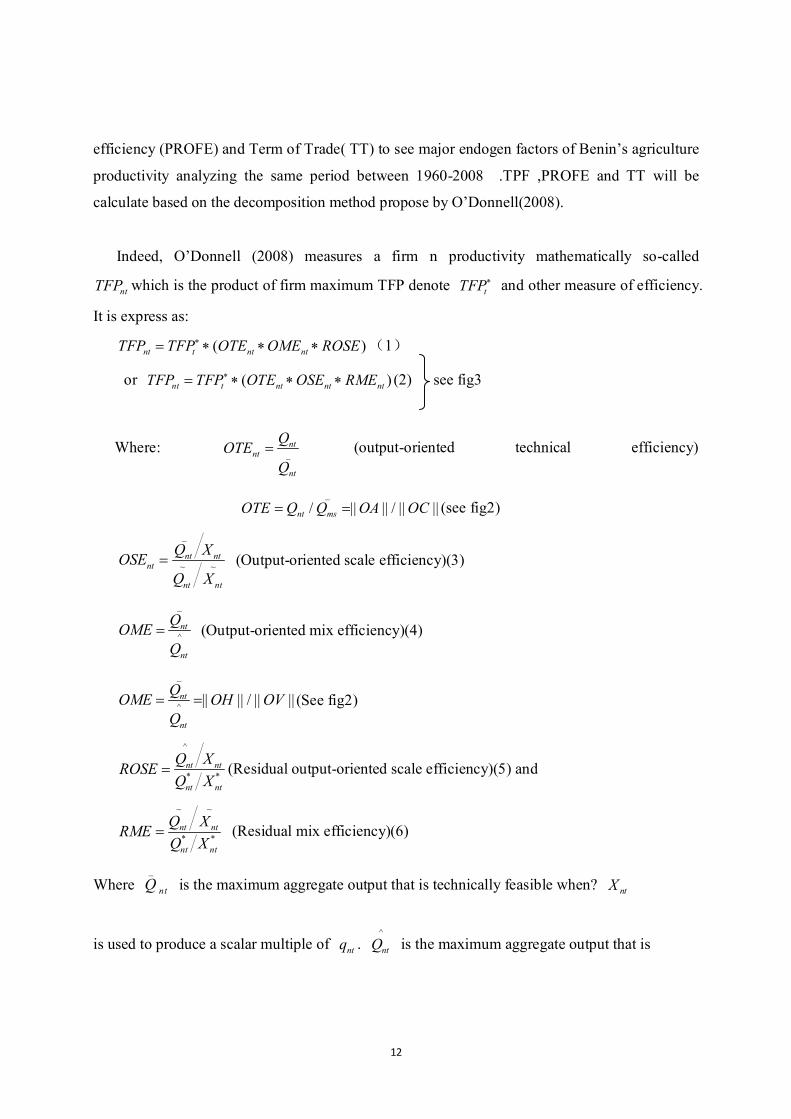
Where _

ntQ is the maximum aggregate output that is technically feasible when? ntX

is used to produce a scalar multiple of ntq . ^

ntQ is the maximum aggregate output that is

13

feasible when using ntX to produce any output vector; and ~

n tQ and ~

ntX are the aggregate output and input obtained when TFP is maximized subject to the constraint that the output and input vectors are scalar multiples of ntq and ntX respectively

Figure2： Output-oriented measures of efficiency.

Figure3： Output-oriented measures of efficiency

A similar equation holds for firm m in period s. It follows that the index that compares the TFP

of firm n in period t with the TFP of firm m in period s can be writing

14

*

, *( ) ( )nt t nt nt ntms nt

ms s ms ms ms

TFP TFP OTE OME ROSETFPTFP TFP OTE OME ROSE

(7)

*

*( ) ( )t nt nt nt

s ms ms ms

TFP OTE OSE RMETFP OTE OSE RME

(8)

Figure4: Technical changes.

Each TFP and other efficiency will be compute applying the DPNI software writing by

O’Donnell (2008) base on Data Envelopment Analysis using the country agriculture input and

output data collected in first part.

Moreover, the profitability amount firm n in period t and firm m in period s is express as the

product of TT and TFP. Mathematically, we have:

, ,, , ,

, ,

ms nt ms ntntms nt ms nt ms nt

ms ms nt ms nt

P QPROFPROF TT TFPPROF W X

PROF is computing directly using the DPIN. From this it is easy to deduce the Terms of

Trade. There is an inverse relationship between productivity and the terms of trade which holds

two interesting implications. First, it provides a rationale for microeconomic reform programs

designed to increase levels of competition in agricultural output and input markets –

deteriorations in the terms of trade that result from increased competition will tend to drive firms

15

towards points of maximum productivity. Second, it provides an explanation for the observed

convergence in rates of agricultural productivity growth in regions, states and countries that are

becoming increasingly integrated and/or globalised – firms that strictly prefer more income to

less and who face the same technology and prices will optimally choose to operate at the same

point on the production frontier, they will make similar adjustments to their production choices

in response to changes in the common terms of trade, and they will thus experience similar rates

of productivity change.

3-Result and Discussion

Benin has done a great effort since several years to achieve the country food demand. This is

showed by the country grain, vegetable and meat output and output per ha variation since 1961.

Grain Production

In Benin grain production is characterize by maize, rice, sorghum and millet. Maize is the major

grain crop production in Benin and its large number of varieties allows the production under

climatic conditions reaching from sub humid to semi-arid. It grows in all parts in the country

rotationally depending on the local consumption patterns and comparative advantages of other

products (Valerien O. Pede, 2005) mostly grow maize is most grow in the south region.

Grain output generally has increased slowly from 1960 until today with some fall and maize

is the highest output production. While the output per ha has also increase slowly since 1960

with major fall in 1977, 1988 and 2008.This is illustrated by the graph2a and graph2b below.

Vegetable and fruit output has also known slow increased from 1961 with the higher pick in

1990(500000 MT) of fruit. Idem for the output per ha which fall since 1996 until today.

Over all the period fruit production output is higher than vegetable. This illustrated by the

graph3a and graph3b below.

Meat production output rise since 1961 until nowadays in average but with constant

production from 1963to 1986 (2000MT) before to rose, while the meat output per capita has

16

decreased from 1966(13T/ha) to 1986(8T/ha) before to rise. This is illustrated by the

graph4a and graph4b below.

Cash crop production has also fluctuate over the whole period with slow rise since 1961,

two pick in 1997 and 2005 before to fall since 2005.Cotton seed was more important in term

of quantity than palm oil. This is demonstrated by the graph5a and graph5b below. Indeed,

there is inverse relationship between palm kernel and palm oil. This is emphasized by the

graph5c below.

However, this cannot be achieved without input improvement. Agriculture labor, land, fertilizer

and machines used have fluctuated significantly over the years.

Agricultural lands have considerably increased from 1961 at 2005 and fall slowly since

2005.This is emphasized by the graph6 below.

Agriculture machine has significantly decreased from 1961(0.75 tractor per 100km) to

1978(0.65 tractor per 100km) and increased from 1978 to his pick in 1 tractor per 100 km in

1996 before to fall until 2000 to his constant level. This is presented by the graph7 below.

Fertilizers used over all the period varied in switchback. This describe by the graph8a and

graph8b below.

Labor in general has increased considerably over the period. This is emphasized by the

graph9.

In general, it is fund that over decades Benin agriculture grain has increased, while vegetable

output per ha decreased and livestock per ha increased. Look at the variation of Benin agriculture

input, it could be concluded that all the production has been achieved using very intensive labor.

Land expansion increased but the mechanization is still very archaic with high punt of fertilizer

used.

Graph2a: Benin Grain Output Variation between 1961 and 2008

17

Grain Output

0200000400000600000800000

1000000120000014000001600000

1961

1964

1967

1970

1973

1976

1979

1982

1985

1988

1991

1994

1997

2000

2003

2006

2009

years

MT(Mille Ton)

Sorghum

Millet

Maize

Rice Paddy

Source: Emphasize is mine from FAO statistical database

Graph2b: Benin Grain Output per ha Variation between 1961 and 2008

Grain output per ha

050

100150200250300350400

1961

1964

1967

1970

1973

1976

1979

1982

1985

1988

1991

1994

1997

2000

2003

2006

years

T/ha

Sorghum

Millet

Maize

Rice


Graph3a: Benin Vegetable Output Variation between 1961 and 2008

Vegetable-fruit otal output

0

100000

200000

300000

400000

500000

600000

1961

1966

1971

1976

1981

1986

1991

1996

2001

2006

years

MT Fruit fresh nes

Vegetables fresh nes


18

Graph3b: Benin Vegetable Output per ha Variation between 1961 and 2008

Vegetable output per ha

0

50

100

150

200

250

1961

1964

1967

1970

1973

1976

1979

1982

1985

1988

1991

1994

1997

2000

2003

2006

years

T/ha Fruit fresh nes

Vegetables fresh nes


Graph4a: Benin Meat Output Variation between 1961 and 2008

Meat Total Output

01000020000

3000040000500006000070000

1962

1966

1970

1974

1978

1982

1986

1990

1994

1998

2002

2006

year

MT

Indigenous Chickenmeat

Indigenous cattlemeat

egs,milk


Graph4b: Benin Meat Output per ha Variation between 1961 and 2008

19

Meat Output per ha

0

5

10

15

20

25

1962

1966

1970

1974

1978

1982

1986

1990

1994

1998

2002

2006

years

T/ha

Indigenous Chickenmeat

Indigenous cattlemeat

egs,milk

Source: Emphasize is mine from FAO statistical database.

Graph5a: Benin Cash Crop Output Variation between 1961 and 2008

Cash crop Output

0

50000100000

150000200000

250000300000350000

1961

1965

1969

1973

1977

1981

1985

1989

1993

1997

2001

2005

2009

Years

MT

Palm seed

Cotton seed


20

Graph5b: Benin Cash Crop Output Variation between 1961 and 2008

Cash crop output per ha

0

20

40

60

80

100

1961

1964

1967

1970

1973

1976

1979

1982

1985

1988

1991

1994

1997

2000

2003

2006

years

T/h

a Palm seed

Cotton seed


Graph5c: Benin Kernel-Plam oil Output Variation between 1961 and 2008

Palm kernel seed- palm oil

0

10

20

30

40

50

1961

1965

1969

1973

1977

1981

1985

1989

1993

1997

2001

2005

2009

years

MT

Palm seed

Palm oil


21

Graph6: Benin Agricultural Land Variation between 1961 and 2008

agricultural land area

05001000150020002500300035004000

1961

1965

1969

1973

1977

1981

1985

1989

1993

1997

2001

2005

2009

years

1000ha

Land(1000ha)


Graph7: Benin Agricultural Machine Used Variation between 1961 and 2008

agriculture Machine tra(sq 100km)

0

0.2

0.4

0.6

0.8

1

1.2

1961

1966

1971

1976

1981

1986

1991

1996

2001

2006

years

Number of machine

tractor per 1000Km

Mach tra(sq 100km)


Graph8a: Benin Fertilizer Used Variation between 1961 and 2008

22

Fertilizer use(Tonne metric)

0

10000

20000

30000

40000

50000

60000

1961

1966

1971

1976

1981

1986

1991

1996

2001

2006

years

Metric tonne

Fertilizeruse(Tonne metric)


Graph8b: Benin Fertilizer Used per ha Variation between 1961 and 2008

Fertilizer use per ha

0

5

10

15

20

1961

1965

1969

1973

1977

1981

1985

1989

1993

1997

2001

2005

2009

years

metr

ic ton

ne per

ha

Fertilizer use perha


Graph9: Benin Agricultural Labor Forces Variation between 1961 and 2008

23

agriculture labor forces

0

1000

2000

3000

4000

5000

1961

1965

1969

1973

1977

1981

1985

1989

1993

1997

2001

2005

2009

years

Man day

系列1


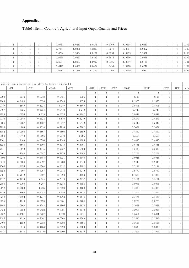
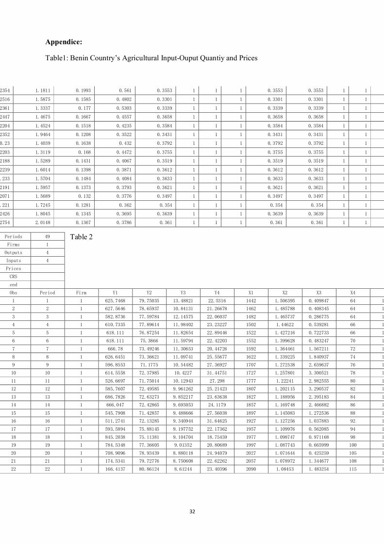
Moreover indexes that measure change in Benin agricultural profitability (PROF), productivity

(TFP) and term of trade (TT) variation between the review period has been very remarkable

presented .This is illustrated by figure5 and figure6 below. Both figure are obtain using the DPIN

result presented in appendices Table1 and Table2.

The Analysis of Fig5, analysis showed that Profitability decreased by 77, 55% from 1961 to

1990 before the agriculture liberalization and increased by 22.67% between 1990 and 2008 after

the liberalization. However Productivity increased by 77.99% between 1961 and 1990 and

decreased at 31.68% during 1990-2008 while the Term of trade increased at 12.19% during

1961-1990 and increased by 79.58% between 1990 and 2008.

This is consistent with the inverse relationship between productivity and terms of trade. The

improvement of term of trade in Benin explain the lack of competiveness in the sector and the

increased of agriculture profitability while the productivity decreased significantly.

In a related development, it justifies the conclusion that over the period of liberalization of the

agriculture sector during 1990, there has been limited private sector involvement and investment.

It is also consistent with this finding that the big gap that we can observe result in agriculture

output prices that are much higher that agriculture input prices and with the global economic

crisis the figures take on a deeper meaning.

24

Moreover, evidence of this type of optimizing duality response can be observed regarding the

index of technical change and output- oriented efficiency change presented in Fig6:

It can be seen that important components of Benin agricultural TFP change have been change in

OSME= OME* ROSE but not change in Technical Change. Meaningful, OME and ROSE have

been important index in TFP change index.

Indeed, an average of OME and ROSE has felled since 1961 during the pre reform and felled

more during the post reform. OME and ROSE failed by 60.82% between 1961 and 1990 and by

55.7% between 1990 and 2008.

We can conclude that the decreased of productivity during the post reform has not been due to

any change of Benin agricultural producer production ability but due to multiples lack of good

management.

Figure5: Indexes Measuring Changes in Profitability, TFP and the Terms of Trade in Benin

Agricultural.

25

Figure6: Output-Oriented Components of TFP Change

4-Conclusion

It can be concluded that during the period after independence (1961), Benin’s agricultural

productivity fell and that fall took on more significance after the beginning of the openness

period (economic reform period in1990). However, since 1990, the term of trade has strongly

extremely improved due to a lack of competiveness. Indeed, very limited private involvement in

the sector has led the sector to be more protectionists with profit taking prominence over

developing economic potential in the sector. This explains the low private investment in the

agriculture sector and the necessity of urgent policy action to be taken by government in the

sector, particularly in light of the recent food crisis in 2008.Agricultural liberalization does not

assist Benin to improve food production or to encourage sustainable development of the sector –

a sector key to Benin’s economic growth.

26

5-References [1]-Alejandro, N. P. and Bingxin, Y. (2008). “ An Updated Look at The Recovery of Agriculture

Productivity in Sub-Sahara Africa”. IFPRI Discussion Paper 00787 August 2008.

[2]-Adekambi, S.; Adegbola, P. ; Gelele, E.; Agli, C. K. et Tamegno, B. (2010), “ Contribution

of agricultural technology to productivity improvement: case study of high yield cassava

varieties in Benin,’’.Contributed Paper presented at the Joint 3rd African Association of

Agricultural Economists (AAAE) and 48th Agricultural Economists Association of South

Africa (AEASA) Conference, Cape Town, South Africa, September 19-23, 2010.

[3]-BAfD/OCDE report (2008). Perspectives Economiques en Afrique. OCDE, Paris, P165-176.

Ministère de l’Agriculture, de l’Elevage et de la Pêche , (MAEP) (2009). Mise en Place d’un

Model D’équilibre Sectorielle Pour L’analyse De La Politique Agricoles Au Benin,

September 2009.

[4]-Carlos, E. L. (2010). “Agricultural Productivity Growth, Efficiency Change and Technical

Progress in Latin America and the Caribbean”. Inter-American Development Bank (IDB)

working paper series186. May 20102010.

[5]-Coelli, T.J., Prasada Rao, D.S., and Battese, G.E. (1998), An Introduction to Efficiency and

Productivity Analysis, Kluwer Academic Publishers, Boston, 271 pp.

[6]-Chambers, R. G. 1988. Applied production analysis, a dual approach. Cambridge University Press, New York. 331 p.

[7]-Coelli, T., Rao, D. and Battese, G. (2005). “An Introduction to Efficiency and Productivity

Analysis.”, Books Second Edition, New York: Springer publisher.

[9]-Caves, D. W, Christensen, Laurits ,R . Diewert, W. E.( 1982). “The Economic Theory of

Index Numbers and the Measurement of Input, Output, and Productivity,”. Econometrica,

Econometric Society, vol. 50(6), pages 1393-1414, November.

[10]-David, K. and Elliott, P.(1998 ).“Productivity in Chinese Provincial Agriculture”. Journal

of Agricultural Economics Volume 49, Issue 3, pages 378–392, September 1998. Article first

published online: 5 NOV 2008 DOI: 10.1111/j.1477-9552.1998.tb01279.

[11]-Equipe Sectoriel de Contrepartie Du Benin (ESC)(2004) . Strategy Sectoriel De Developpement et De La Promotion Des Exportations & Et Plan D’action Marketing Export du Secteur Manioc. http://www.abepec.bj/Strat%E9gie%20fili%E8re%20maniocREVIM_1.pdf

[12] Fare, R., (1988). “Fundamental of production theory”. Heidelberg : Springer-Verlag.

[13]-Fa re, R., Grosskopf, S., Norris, M. and Zhang, Z. (1994). “Productivity growth, technical

27

progress, and efficiency change in industrialized countries”. American Economic Review

84(1),66–83.

[14]-Gboyega, A. O(2000) . “Concept and Measurement Of Productivity”. Department of Economics University of Ibadan Ibadan. http://www.mendeley.com/research/concept-measurement-productivity-4/#page-1

[15]-Grosskopf, S. (1993). “Efficiency and Productivity” in Fried, H.O, Knox, C. L. L. and

Shelton, S. S ‘The Measurement of Productive Efficiency: Techniques and Applications’.

New York : Oxford University Press, pp. 160-194.

[16]-Joseph, P. (1987). International Labour Office Productivity management: a practical

handbook, Page 94. Business & Economics - 287 pages

[17]-Laurenceson J., O’Donnell, & C.J. 2011. New Estimates and a Decomposition of Provincial Productivity Change in China," CEPA Working Papers Series WP042011, School of Economics, University of Queensland, Australia.

[18]-Ministere De L’Agriculture, De L’Elevage Et De La Peche –Ministere Du Developpement De L’Economie Et Des Finance (MAEP-MDEF, 2006) .Stratégie Pour L’Atteinte De L’Objectif N°1 Des OMD Au BENIN , Décembre 2006 http://www.bj.undp.org/docs/omd/OMD_Agriculture.pdf

[19]-MAEP (2010). “Rapport De L’etude Pour La Proposition Du Prix Plancher Du Cotton

Graine Campagne 2010-2011”. Office National De Soutien Des Revenue Agricole.

[20]-MFE (2010), “Evaluation Ex-Ante De La Mise En ŒUVRE Des Stratégie De

Relance Du Pole Coton-Textile Au BENIN’’.

[21]-Michael A. Trueblood , Jay Coggins. “Intercountry Agiculture Efficiency and Productivity: Malquist Index Approach.”U.S. Dept. of Agriculture, Economic Research Service and University of Minnesota, Dept. of Applied Economics http://faculty.apec.umn.edu/jcoggins/documents/Malmquist.pdf

[22]-Moussaratou, S.(2008). “Déterminants du prix de la terre agricole au Bénin ”.

Institut de l’économie agro-alimentaire et des ressources naturelles, Université de Bonn I M

P E T U S Sous-projet B4 - 03/2008.

[23]-Nicolas, P. (2011), “Durabilité et productivité: Une introduction au Système Better Cotton’’.

Gestionnaire de Programme Afrique et Amérique latine – BCI 27 Juin 2011, Cotonou –

Benin,Better Cotton Initiative(BCI) Working Paper.

[24]-Nin, A., C. Arndt, T.W. Hertel, and P.V. Preckel et al. 2003. “Bridging the Gap between Partial and Total Factor Productivity Measures using Directional Distance Functions.” American Journal of Agricultural Economics 85(4): 928-942.

28

[25]-O'Donnell, Christopher J. & Coelli, Timothy J., 2005. "A Bayesian approach to imposing

curvature on distance functions," Journal of Econometrics, Elsevier, vol. 126(2), pages

493-523, June.

[26]-O’Donnell, C.J. (2008). An aggregate quantity-price framework for measuring and

decomposing productivity and profitability change, Centre for Efficiency and Productivity

Analysis.Working Papers WP07/2008. University of Queensland, Queensland.

[27]-O’Donnell C.J. (2010) “Nonparametric Estimates Of The Components Of Productivity

And Profitability Change In U.S. Agriculture”.Centre for Efficiency and Productivity

Analysis Working Paper Series No. WP02/2010.

[28]-O’Donnell, C.J. (2010). DPIN Version 1.0: a program for decomposing productivity index

numbers. Centre for Efficiency and Productivity Analysis Working Papers WP01/2010.

University of Queensland, Queensland.

[29]-Shih-Hsun , H., Ming-Miin, Y. and Ching-Cheng, C.(2003). “An Analysis of Total Factor

Productivity Growth in China’s Agricultural Sector”. Paper prepared for presentation at the

American Agricultural Economics Association Annual Meeting, Montreal, Canada, July

27-30, 2003.

[30]-Shephard, R. W., (1970). “Theory of cost and production functions”. Princeton: Princeton

University Press,

[31]-Sekloka, E. , Hougni, A. , Katary .A., Djaboutou M.and J. Lançon,(2009). “ I 875.3 et H

769.5 variétés prometteuses de coton (Gossypium hirsutum L.) sélectionnées au Bénin ’’.

Benin : Bulletin de la Recherche Agronomique du Bénin Numéro 63 – Mars 2009.

[32]-Tim Coelli & Shannon Walding, 2005. "Performance Measurement in the Australian Water Supply Industry," CEPA Working Papers Series WP012005, School of Economics, University of Queensland

[33]-Valerien,O. P. and Andrew, M. M. (2005). “Integration In Benin Maize Market: An Application OF Threshold Cointegration Analysis” Presentation Paper during the American Agricultural Economics Association Annual Meeting, Providence, Rhode Island, July 24-27, 2005.

[34]-Vu Hoang Linh,( 2003). “Vietnam’s Agriculture Productivity: A Malquist Index Approach”.

VDF Working Paper 090.

29

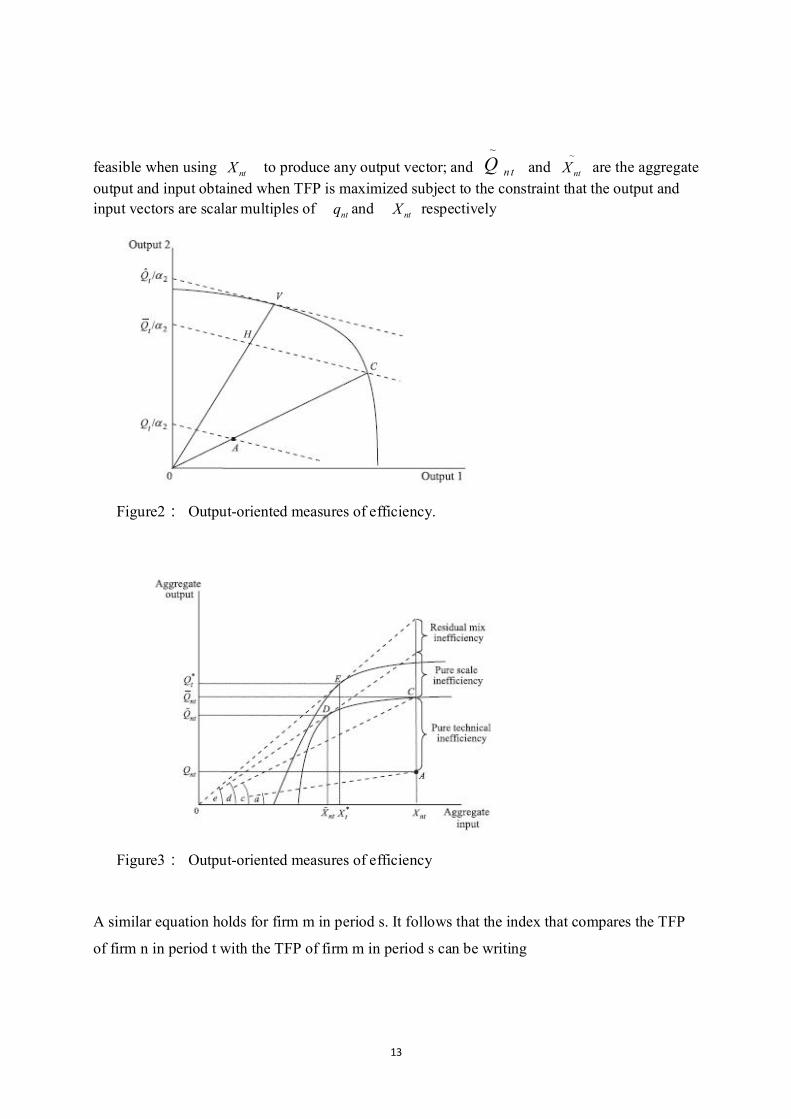
Appendice:

Table1: Benin Country’s Agricultural Input-Ouput Quantiy and Prices

30

Hicks-Moorsteen Indexes: firm n in period t relative to firm n in period t-1

OTE OSE OME ITE ISE IME MaxTFP dPROF dTT dTFP dTech dEff dOTE dOSE dOME dROSE

1 1 1 1 1 1 1.7386

1 1 1 1 1 1 1.6432 0.9799 1.0914 0.8978 0.9451 0.95 1 1 1 0.95

1 1 1 1 1 1 1.6591 0.9398 0.7774 1.209 1.0097 1.1974 1 1 1 1.1974

1 1 1 1 1 1 1.6603 1.0184 1.3609 0.7483 1.0007 0.7478 1 1 1 0.7478

1 1 1 1 1 1 1.6374 1.003 1.155 0.8684 0.9862 0.8805 1 1 1 0.8805

1 1 1 1 1 1 1.63 0.9566 0.814 1.1752 0.9955 1.1805 1 1 1 1.1805

1 1 1 1 1 1 1.523 1.0353 1.856 0.5578 0.9343 0.597 1 1 1 0.597

1 1 1 1 1 1 1.4912 0.9302 0.9215 1.0094 0.9791 1.0309 1 1 1 1.0309

1 1 1 1 1 1 1.3801 0.9223 1.0713 0.861 0.9255 0.9303 1 1 1 0.9303

1 1 1 1 1 1 1.3724 1.0114 1.0511 0.9622 0.9944 0.9677 1 1 1 0.9677

1 1 1 1 1 1 1.2725 0.8448 0.8838 0.9559 0.9272 1.0309 1 1 1 1.0309

1 1 1 1 1 1 1.2775 1.069 1.0986 0.9731 1.0039 0.9693 1 1 1 0.9693

1 1 1 1 1 1 1.416 1.1269 0.9282 1.2141 1.1085 1.0953 1 1 1 1.0953

1 1 1 1 1 1 1.3834 0.9531 0.9644 0.9882 0.9769 1.0115 1 1 1 1.0115

1 1 1 1 1 1 1.3873 0.824 0.6187 1.3319 1.0029 1.3281 1 1 1 1.3281

1 1 1 1 1 1 1.3945 0.9209 0.8199 1.1232 1.0052 1.1174 1 1 1 1.1174

1 1 1 1 1 1 1.4401 1.1005 0.9076 1.2125 1.0327 1.1741 1 1 1 1.1741

1 1 1 1 1 1 1.5877 1.3295 1.5844 0.8391 1.1025 0.7611 1 1 1 0.7611

1 1 1 1 1 1 1.5778 0.9216 0.7597 1.2131 0.9938 1.2207 1 1 1 1.2207

1 1 1 1 1 1 1.5464 0.8851 0.6964 1.271 0.9801 1.2969 1 1 1 1.2969

1 1 1 1 1 1 0.9415 0.3123 1.1173 0.2795 0.6088 0.4591 1 1 1 0.4591

1 1 1 1 1 1 0.9107 0.9274 0.9832 0.9432 0.9673 0.9751 1 1 1 0.9751

1 1 1 1 1 1 0.9614 1.0076 1.1955 0.8428 1.0556 0.7984 1 1 1 0.7984

1 1 1 1 1 1 0.9492 1.1724 1.2667 0.9256 0.9874 0.9374 1 1 1 0.9374

1 1 1 1 1 1 0.9323 1.0622 1.1542 0.9203 0.9821 0.9371 1 1 1 0.9371

1 1 1 1 1 1 0.9668 0.9203 0.8428 1.092 1.037 1.053 1 1 1 1.053

1 1 1 1 1 1 0.8353 0.7974 0.9575 0.8328 0.864 0.9638 1 1 1 0.9638

1 1 1 1 1 1 1.0747 1.2858 0.9254 1.3894 1.2865 1.08 1 1 1 1.08

1 1 1 1 1 1 1.6134 1.0481 0.4875 2.1501 1.5013 1.4321 1 1 1 1.4321

1 1 1 1 1 1 0.9672 0.8797 2.2893 0.3842 0.5995 0.641 1 1 1 0.641

1 1 1 1 1 1 1.0411 1.073 0.9946 1.0788 1.0764 1.0023 1 1 1 1.0023

1 1 1 1 1 1 0.9387 0.9753 1.1785 0.8276 0.9017 0.9178 1 1 1 0.9178

1 1 1 1 1 1 1.0268 1.0546 0.9073 1.1624 1.0939 1.0626 1 1 1 1.0626

1 1 1 1 1 1 0.9754 0.9502 0.9899 0.9599 0.9499 1.0106 1 1 1 1.0106

1 1 1 1 1 1 0.8349 1.069 1.3441 0.7953 0.856 0.9291 1 1 1 0.9291

1 1 1 1 1 1 0.922 0.9384 0.8401 1.117 1.1044 1.0114 1 1 1 1.011

1 1 1 1 1 1 0.7924 1.0362 1.1003 0.9417 0.8594 1.0957 1 1 1 1.0957

1 1 1 1 1 1 0.7363 0.901 0.9898 0.9103 0.9292 0.9796 1 1 1 0.9796

1 1 1 1 1 1 0.6123 1.0669 1.3401 0.7961 0.8315 0.9574 1 1 1 0.9574

1 1 1 1 1 1 0.751 0.9778 0.7213 1.3556 1.2267 1.1051 1 1 1 1.1051

1 1 1 1 1 1 0.7776 0.9582 0.9344 1.0254 1.0354 0.9904 1 1 1 0.9904

1 1 1 1 1 1 0.7071 0.9932 1.1654 0.8522 0.9094 0.9371 1 1 1 0.9371

Appendice:


31

1 1 1 1 1 1 0.6731 1.0233 1.0475 0.9769 0.9518 1.0263 1 1 1 1.0263

1 1 1 1 1 1 0.7101 1.0406 0.9806 1.0611 1.0551 1.0057 1 1 1 1.0057

1 1 1 1 1 1 0.6594 0.9404 1.0161 0.9255 0.9285 0.9967 1 1 1 0.9967

1 1 1 1 1 1 0.6565 0.9453 0.9832 0.9615 0.9956 0.9658 1 1 1 0.9658

1 1 1 1 1 1 0.6294 1.0667 1.0992 0.9705 0.9587 1.0123 1 1 1 1.0123

1 1 1 1 1 1 0.6425 1.0981 1.0464 1.0493 1.0208 1.0279 1 1 1 1.0279

1 1 1 1 1 1 0.6582 1.1349 1.1165 1.0165 1.0245 0.9922 1 1 1 0.9922

Moorsteen Indexes: firm n in period t relative to firm n in period 1

dTT dTFP dTech dEff dOTE dOSE dOME dROSE dOSME dITE dISE dIME

1 1 1 1 1 1 1 1 1 1 1 1

0.9799 1.0914 0.8978 0.9451 0.95 1 1 1 0.95 0.95 1 1

0.9209 0.8484 1.0855 0.9543 1.1375 1 1 1 1.1375 1.1375 1 1

0.9379 1.1546 0.8123 0.955 0.8506 1 1 1 0.8506 0.8506 1 1

0.9407 1.3335 0.7054 0.9418 0.749 1 1 1 0.749 0.749 1 1

0.8999 1.0855 0.829 0.9375 0.8842 1 1 1 0.8842 0.8842 1 1

0.9316 2.0148 0.4624 0.876 0.5279 1 1 1 0.5279 0.5279 1 1

0.8666 1.8567 0.4667 0.8577 0.5442 1 1 1 0.5442 0.5442 1 1

0.7993 1.989 0.4018 0.7938 0.5062 1 1 1 0.5062 0.5062 1 1

0.8084 2.0906 0.3867 0.7893 0.4899 1 1 1 0.4899 0.4899 1 1

0.6829 1.8478 0.3696 0.7319 0.505 1 1 1 0.505 0.505 1 1

0.7301 2.03 0.3596 0.7348 0.4895 1 1 1 0.4895 0.4895 1 1

0.8228 1.8843 0.4366 0.8145 0.5361 1 1 1 0.5361 0.5361 1 1

0.7841 1.8172 0.4315 0.7957 0.5423 1 1 1 0.5423 0.5423 1 1

0.6461 1.1243 0.5747 0.7979 0.7203 1 1 1 0.7203 0.7203 1 1

0.595 0.9218 0.6455 0.8021 0.8048 1 1 1 0.8048 0.8048 1 1

0.6548 0.8366 0.7827 0.8283 0.9449 1 1 1 0.9449 0.9449 1 1

0.8706 1.3255 0.6568 0.9132 0.7192 1 1 1 0.7192 0.7192 1 1

0.8023 1.007 0.7967 0.9075 0.8779 1 1 1 0.8779 0.8779 1 1

0.7101 0.7012 1.0127 0.8894 1.1386 1 1 1 1.1386 1.1386 1 1

0.2217 0.7835 0.283 0.5415 0.5227 1 1 1 0.5227 0.5227 1 1

0.2056 0.7703 0.267 0.5238 0.5096 1 1 1 0.5096 0.5096 1 1

0.2072 0.9209 0.225 0.5529 0.4069 1 1 1 0.4069 0.4069 1 1

0.2429 1.1664 0.2083 0.546 0.3814 1 1 1 0.3814 0.3814 1 1

0.258 1.3462 0.1917 0.5362 0.3574 1 1 1 0.3574 0.3574 1 1

0.2375 1.1346 0.2093 0.5561 0.3764 1 1 1 0.3764 0.3764 1 1

0.1893 1.0863 0.1743 0.4805 0.3628 1 1 1 0.3628 0.3628 1 1

0.2434 1.0053 0.2422 0.6181 0.3918 1 1 1 0.3918 0.3918 1 1

0.2552 0.4901 0.5207 0.928 0.5611 1 1 1 0.5611 0.5611 1 1

0.2245 1.1219 0.2001 0.5563 0.3596 1 1 1 0.3596 0.3596 1 1

0.2409 1.1159 0.2158 0.5988 0.3605 1 1 1 0.3605 0.3605 1 1

0.2349 1.315 0.1786 0.5399 0.3308 1 1 1 0.3308 0.3308 1 1

0.2477 1.1932 0.2076 0.5906 0.3515 1 1 1 0.3515 0.3515 1 1

Appendice:


32

0.2354 1.1811 0.1993 0.561 0.3553 1 1 1 0.3553 0.3553 1 1

0.2516 1.5875 0.1585 0.4802 0.3301 1 1 1 0.3301 0.3301 1 1

0.2361 1.3337 0.177 0.5303 0.3339 1 1 1 0.3339 0.3339 1 1

0.2447 1.4675 0.1667 0.4557 0.3658 1 1 1 0.3658 0.3658 1 1

0.2204 1.4524 0.1518 0.4235 0.3584 1 1 1 0.3584 0.3584 1 1

0.2352 1.9464 0.1208 0.3522 0.3431 1 1 1 0.3431 0.3431 1 1

0.23 1.4039 0.1638 0.432 0.3792 1 1 1 0.3792 0.3792 1 1

0.2203 1.3119 0.168 0.4472 0.3755 1 1 1 0.3755 0.3755 1 1

0.2188 1.5289 0.1431 0.4067 0.3519 1 1 1 0.3519 0.3519 1 1

0.2239 1.6014 0.1398 0.3871 0.3612 1 1 1 0.3612 0.3612 1 1

0.233 1.5704 0.1484 0.4084 0.3633 1 1 1 0.3633 0.3633 1 1

0.2191 1.5957 0.1373 0.3793 0.3621 1 1 1 0.3621 0.3621 1 1

0.2071 1.5689 0.132 0.3776 0.3497 1 1 1 0.3497 0.3497 1 1

0.221 1.7245 0.1281 0.362 0.354 1 1 1 0.354 0.354 1 1

0.2426 1.8045 0.1345 0.3695 0.3639 1 1 1 0.3639 0.3639 1 1

0.2754 2.0148 0.1367 0.3786 0.361 1 1 1 0.361 0.361 1 1

Periods 49 Table 2

Firms 1

Outputs 4

Inputs 4

Prices

CRS

end

Obs Period Firm Y1 Y2 Y3 Y4 X1 X2 X3 X4

1 1 1 625.7468 79.75035 13.48821 22.5316 1442 1.506395 0.409847 64 1250

2 2 1 627.5646 78.65937 10.84131 21.26678 1462 1.485788 0.408345 64 1250

3 3 1 582.8736 77.59784 12.14575 22.06037 1482 1.465737 0.286775 64 1250

4 4 1 610.7335 77.89614 11.98402 23.23227 1502 1.44622 0.539281 66 1250

5 5 1 618.111 76.87254 11.82654 22.89446 1522 1.427216 0.722733 66 1250

6 6 1 618.111 75.3866 11.59794 22.42203 1552 1.399628 0.483247 70 1250

7 7 1 666.78 73.49246 11.30653 20.44726 1592 1.364461 1.567211 72 1250

8 8 1 626.6451 73.36621 11.09741 25.55677 1622 1.339225 1.840937 74 1250

9 9 1 596.8553 71.1775 10.54482 27.36927 1707 1.272538 2.659637 76 1250

10 10 1 614.5558 72.37985 10.4227 31.44751 1727 1.257801 3.300521 78 1250

11 11 1 526.6697 71.75014 10.12943 27.298 1777 1.22241 2.982555 80 1250

12 12 1 585.7607 72.49585 9.961262 25.21423 1807 1.202115 3.290537 82 1250

13 13 1 686.7826 72.63273 9.852217 23.63638 1827 1.188956 2.395183 84 1250

14 14 1 666.047 72.42865 9.693053 24.1179 1857 1.169748 2.466882 86 1250

15 15 1 545.7908 71.42857 9.488666 27.56038 1897 1.145083 1.272536 88 1250

16 16 1 511.2741 72.13285 9.340944 31.64625 1927 1.127256 1.037883 92 1250

17 17 1 593.5894 75.88145 9.197752 22.17362 1957 1.109976 0.562085 94 1250

18 18 1 845.2038 75.11381 9.104704 18.75459 1977 1.098747 0.971168 98 1250

19 19 1 784.5348 77.36605 9.01352 20.80689 1997 1.087743 0.665999 100 1250

20 20 1 708.9096 78.93439 8.880118 24.94079 2027 1.071644 0.425259 105 1250

21 21 1 174.5341 79.72776 8.750608 22.62262 2057 1.078972 1.344677 108 1250

22 22 1 166.4137 80.86124 8.61244 23.40396 2090 1.08453 1.483254 115 1250

Appendice:


33

23 23 1 164.9459 100.9524 8.571429 28.98894 2100 1.101852 2.571429 120 1250

24 24 1 209.4328 85.30806 8.530806 40.06186 2110 1.120326 3.488626 125 1250

25 25 1 225.7279 89.20188 11.79343 38.32401 2130 1.134585 5.396244 130 1250

26 26 1 201.4338 86.75799 11.33333 48.68825 2190 1.1276 4.940183 135 1250

27 27 1 162.3612 88.18182 11.28182 30.36816 2200 1.183081 4.304091 140 1250

28 28 1 214.0234 90.04525 16.27149 40.5915 2210 1.24183 3.128507 145 1250

29 29 1 212.5297 229.9505 15.55405 36.76231 2220 1.307558 1.486486 150 1250

30 30 1 199.9544 91.18943 16.07048 45.63608 2270 1.353402 4.847137 155 1250

31 31 1 208.8668 92.54386 19.79386 50.8487 2280 1.419347 5.182895 158 1250

32 32 1 212.2904 93.68192 20.00436 44.43623 2295 1.486323 6.67756 162 1250

33 33 1 213.2632 97.41379 19.93879 67.75316 2320 1.506226 7.430172 165 1250

34 34 1 214.2433 93.33333 19.27417 61.48679 2400 1.490741 7.10625 169 1250

35 35 1 236.8759 92.46032 19.04365 76.9379 2520 1.449515 14.28571 172 1250

36 36 1 214.7541 79.33579 17.70849 95.34483 2710 1.371464 11.3214 175 1250

37 37 1 267.2511 78.27093 16.60554 77.07013 2890 1.306228 13.48374 178 1250

38 38 1 251.6255 66.22951 15.73443 69.72698 3050 1.255009 12.36295 182 1250

39 39 1 286.9905 54.00322 14.37556 72.75471 3110 1.24866 18.23151 182 1250

40 40 1 282.8721 67.50798 14.84632 66.39777 3195 1.235437 11.01721 182 1250

41 41 1 263.353 55.34211 14.50444 75.24594 3265 1.23022 9.525268 182 1250

42 42 1 253.743 51.60297 14.69599 86.52148 3365 1.216774 14.21724 182 1250

43 43 1 284.2468 55.48168 13.80387 73.70984 3467 1.20341 13.79896 182 1250

44 44 1 298.3115 56.30978 15.31427 75.73249 3567 1.191477 13.41211 182 1250

45 45 1 279.6064 55.88182 15.79403 63.96347 3520 1.227904 13.59119 182 1250

46 46 1 241.5542 58.98171 17.18441 64.38562 3335 1.317674 14.34513 182 1250

47 47 1 278.9782 57.81677 17.4021 53.17436 3340 1.336494 14.32365 182 1250

48 48 1 326.4147 60.53019 16.37732 53.01915 3395 1.334479 14.09161 182 1250

49 49 1 380.5201 54.37597 16.37732 56.92685 3300 1.391414 14.49727 182 1250

Documents

Benin Agriculture Productivity and profitability Measurementageconsearch.umn.edu/bitstream/126748/2/9682-RJA1.doc1.pdf · 5 Productivity is defined as the relationship between output