Embed Size (px)
Citation preview
Benefit Cost Analysis Using an Activity-Based Model
TRB Planning Applications Conference
Atlantic City, NJ
May 20, 2015
Joe Castiglione (RSG / SFCTA)
Jeff Frkonja (RSG)
Jim Miller (SANDAG)
22015.05.20RSG
Acknowledgements
SANDAG Clint Daniels Gregor Schroeder Ziying Ouyang
RSG Vince Bernardin Bryce Lovell Mariela Tinarejo
AECOM Toni Horst
32015.05.20RSG
Agenda
SANDAG Projects and Plan Alternatives Evaluation Process
BCA Metrics and Supporting Assumptions BCA Analysis Using SANDAG’s Activity-Based
Model (ABM) Noteworthy Features of BCA based on ABM
42015.05.20RSG
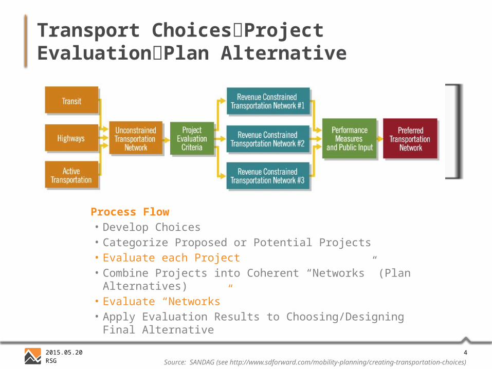
Transport ChoicesProject EvaluationPlan Alternative
Click to add photo
Process Flow• Develop Choices• Categorize Proposed or Potential Projects• Evaluate each Project• Combine Projects into Coherent “Networks” (Plan Alternatives)• Evaluate “Networks”• Apply Evaluation Results to Choosing/Designing Final Alternative
Source: SANDAG (see http://www.sdforward.com/mobility-planning/creating-transportation-choices)
52015.05.20RSG
Benefit-Cost Analysis Overview
Uses monetary value as the metric to support decision-making by making different characteristics comparable
Q: Does an investment (relative to no or different investment) produce more benefits than costs? To invest or not to invest To prioritize investments To better “design” a given investment
Q: Who benefits? Harder to answer this question with past tools
62015.05.20RSG
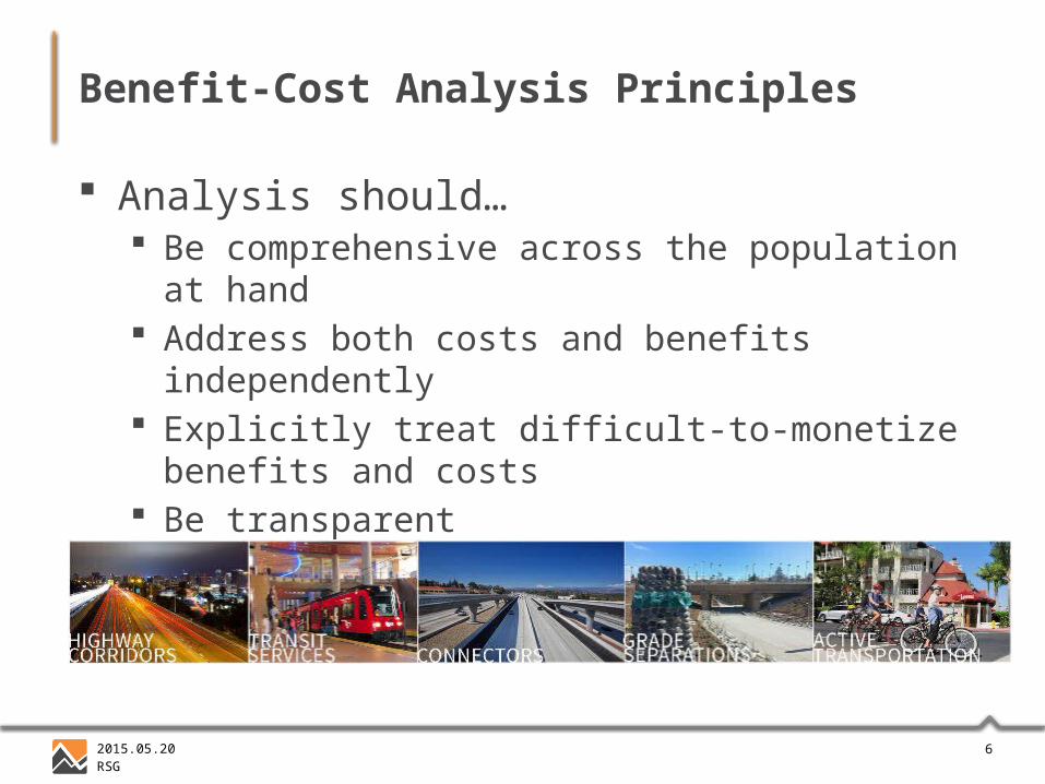
Benefit-Cost Analysis Principles
Analysis should… Be comprehensive across the population at hand Address both costs and benefits independently Explicitly treat difficult-to-monetize benefits and costs Be transparent
72015.05.20RSG
Benefit-Cost Analysis Metrics
Direct benefits Mobility cost savings
Actual travel time savings (residents, trucks) Reliability benefits (residents, trucks)
Vehicle operating cost savings Auto ownership cost savings
Indirect benefits Safety (accident reduction) benefits Emissions (and other environmental) cost savings Physical activity health benefits
82015.05.20RSG
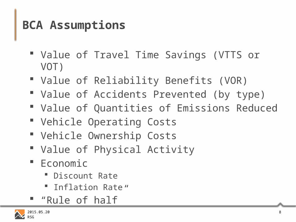
BCA Assumptions
Value of Travel Time Savings (VTTS or VOT) Value of Reliability Benefits (VOR) Value of Accidents Prevented (by type) Value of Quantities of Emissions Reduced Vehicle Operating Costs Vehicle Ownership Costs Value of Physical Activity Economic
Discount Rate Inflation Rate
“Rule of half”
92015.05.20RSG
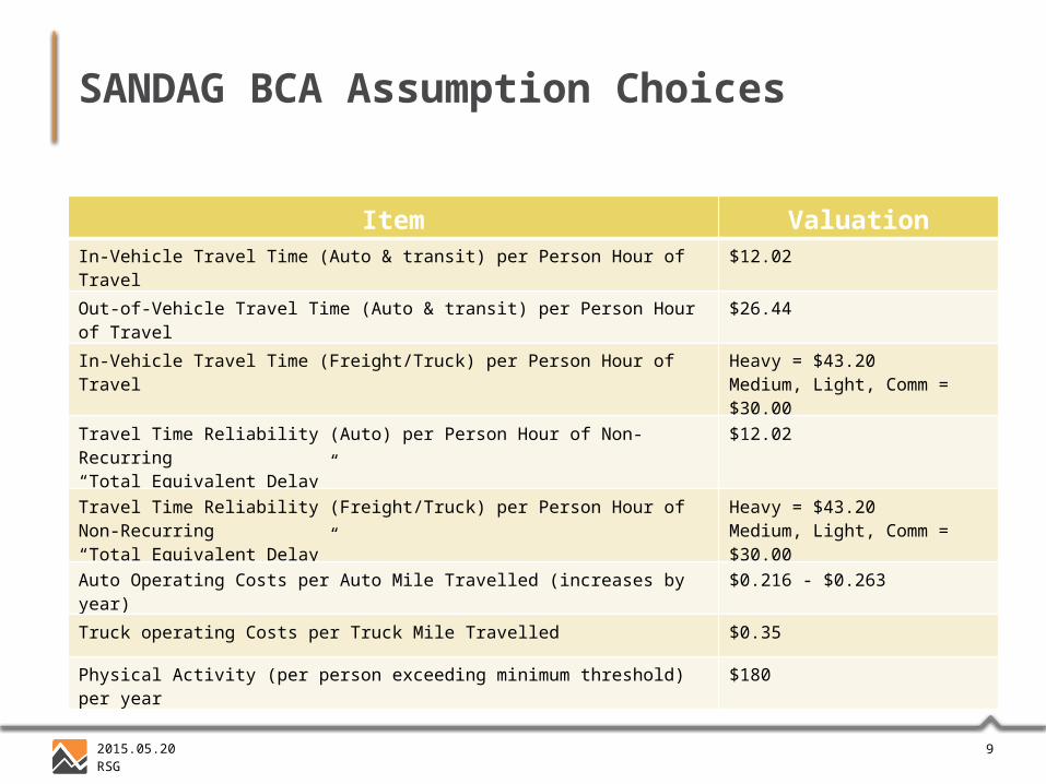
SANDAG BCA Assumption Choices
2010 $Source: SANDAG, RSG. Technical Memorandum “” San Diego Forward Cost Effectiveness Evaluation Criteria Assumptions. 3/6/2014.
Item ValuationIn-Vehicle Travel Time (Auto & transit) per Person Hour of Travel $12.02
Out-of-Vehicle Travel Time (Auto & transit) per Person Hour of Travel $26.44
In-Vehicle Travel Time (Freight/Truck) per Person Hour of Travel Heavy = $43.20Medium, Light, Comm = $30.00
Travel Time Reliability (Auto) per Person Hour of Non-Recurring“Total Equivalent Delay”
$12.02
Travel Time Reliability (Freight/Truck) per Person Hour of Non-Recurring“Total Equivalent Delay”
Heavy = $43.20Medium, Light, Comm = $30.00
Auto Operating Costs per Auto Mile Travelled (increases by year) $0.216 - $0.263
Truck operating Costs per Truck Mile Travelled $0.35
Physical Activity (per person exceeding minimum threshold) per year $180
102015.05.20RSG
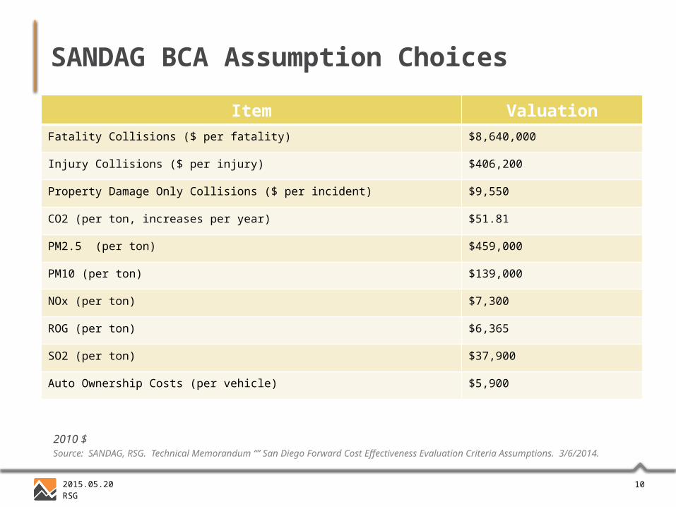
SANDAG BCA Assumption Choices
Item ValuationFatality Collisions ($ per fatality) $8,640,000
Injury Collisions ($ per injury) $406,200
Property Damage Only Collisions ($ per incident) $9,550
CO2 (per ton, increases per year) $51.81
PM2.5 (per ton) $459,000
PM10 (per ton) $139,000
NOx (per ton) $7,300
ROG (per ton) $6,365
SO2 (per ton) $37,900
Auto Ownership Costs (per vehicle) $5,900
2010 $Source: SANDAG, RSG. Technical Memorandum “” San Diego Forward Cost Effectiveness Evaluation Criteria Assumptions. 3/6/2014.
112015.05.20RSG
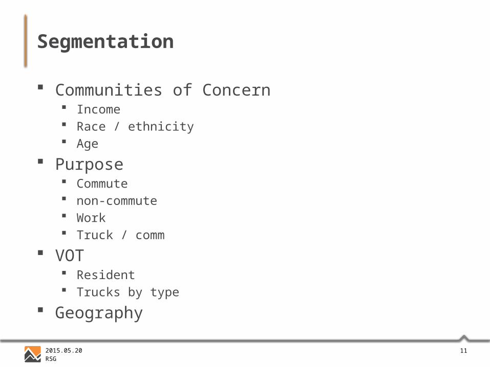
Segmentation
Communities of Concern Income Race / ethnicity Age
Purpose Commute non-commute Work Truck / comm
VOT Resident Trucks by type
Geography
122015.05.20RSG
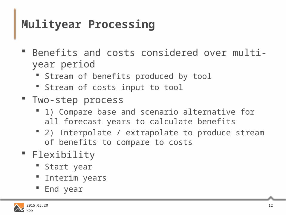
Mulityear Processing
Benefits and costs considered over multi-year period Stream of benefits produced by tool Stream of costs input to tool
Two-step process 1) Compare base and scenario alternative for all forecast years
to calculate benefits 2) Interpolate / extrapolate to produce stream of benefits to
compare to costs
Flexibility Start year Interim years End year
132015.05.20RSG
Multiyear Assumptions
Inflation rate Currency value decline over time
Discount rate Time value of money
Annualization factor
142015.05.20RSG
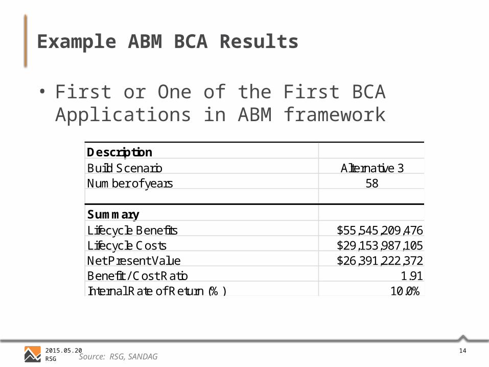
Example ABM BCA Results
• First or One of the First BCA Applications in ABM framework
Source: RSG, SANDAG
DescriptionBuild Scenario Alternative 3Number of years 58
SummaryLifecycle Benefits $55,545,209,476Lifecycle Costs $29,153,987,105Net Present Value $26,391,222,372Benefit / Cost Ratio 1.91Internal Rate of Return (%) 10.0%
152015.05.20RSG
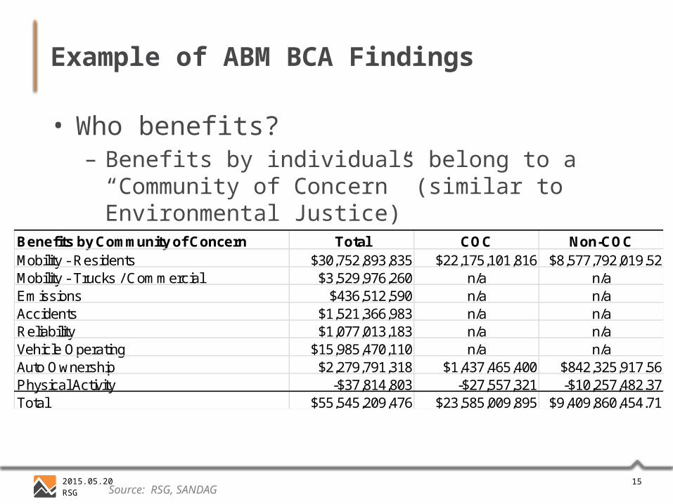
Example of ABM BCA Findings
• Who benefits?– Benefits by individuals belong to a “Community of
Concern” (similar to Environmental Justice)
Source: RSG, SANDAG
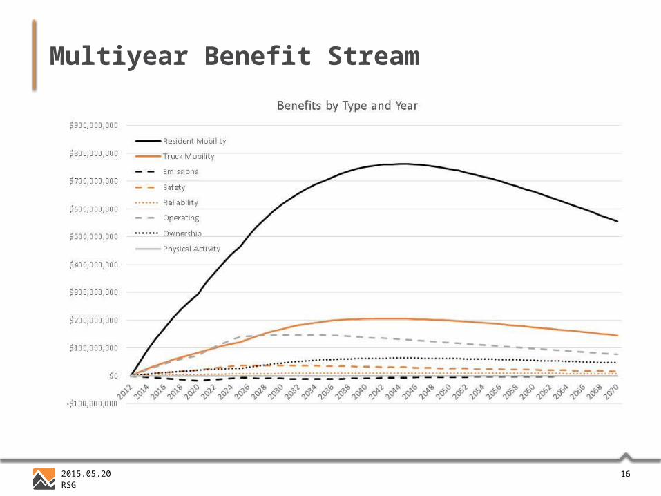
Benefits by Community of Concern Total COC Non-COCMobility - Residents $30,752,893,835 $22,175,101,816 $8,577,792,019.52Mobility - Trucks / Commercial $3,529,976,260 n/a n/aEmissions $436,512,590 n/a n/aAccidents $1,521,366,983 n/a n/aReliability $1,077,013,183 n/a n/aVehicle Operating $15,985,470,110 n/a n/aAuto Ownership $2,279,791,318 $1,437,465,400 $842,325,917.56Physical Activity -$37,814,803 -$27,557,321 -$10,257,482.37Total $55,545,209,476 $23,585,009,895 $9,409,860,454.71
162015.05.20RSG
Multiyear Benefit Stream
172015.05.20RSG
Aggregate vs. Activity-Based Analysis
Aggregate potential level of detail: Zone Market Segment (e.g. Home-Based-Work-Low-
Income)
Activity-based potential level of detail: Person, along any characteristic (e.g. HH income,
age, etc.) Person-trips
182015.05.20RSG
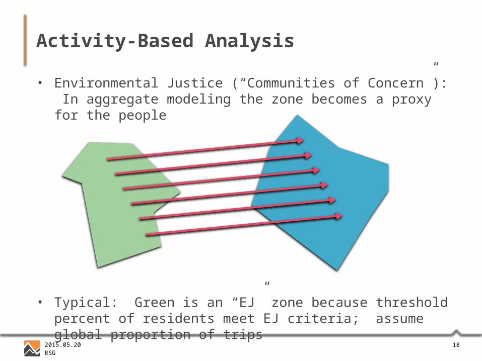
Activity-Based Analysis
• Environmental Justice (“Communities of Concern”): In aggregate modeling the zone becomes a proxy for the people
• Typical: Green is an “EJ” zone because threshold percent of residents meet EJ criteria; assume global proportion of trips
192015.05.20RSG
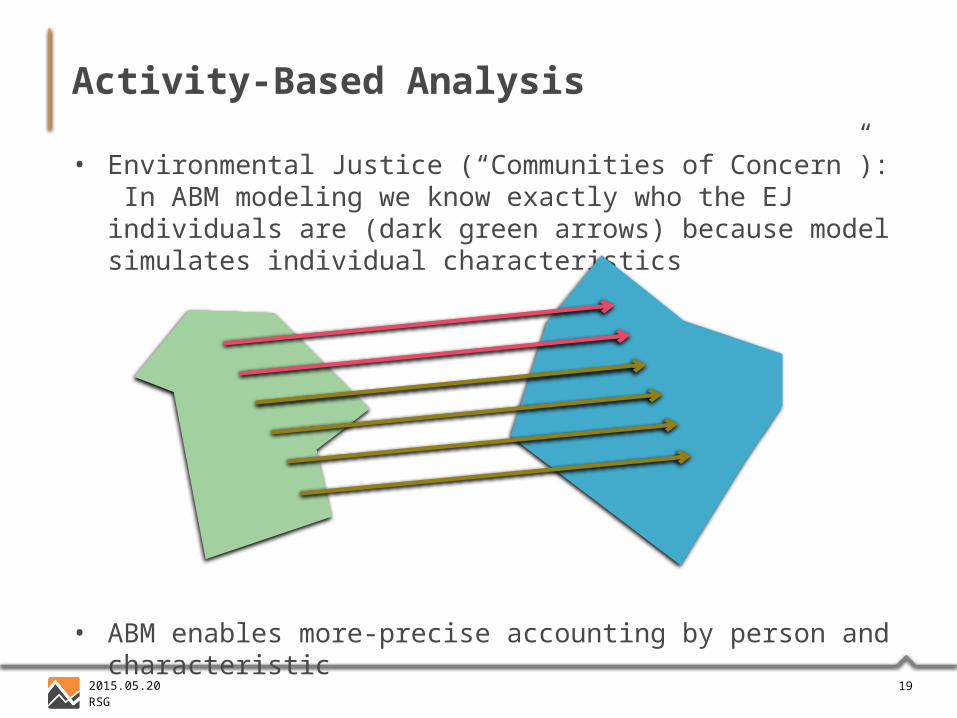
Activity-Based Analysis
• Environmental Justice (“Communities of Concern”): In ABM modeling we know exactly who the EJ individuals are (dark green arrows) because model simulates individual characteristics
• ABM enables more-precise accounting by person and characteristic
202015.05.20RSG
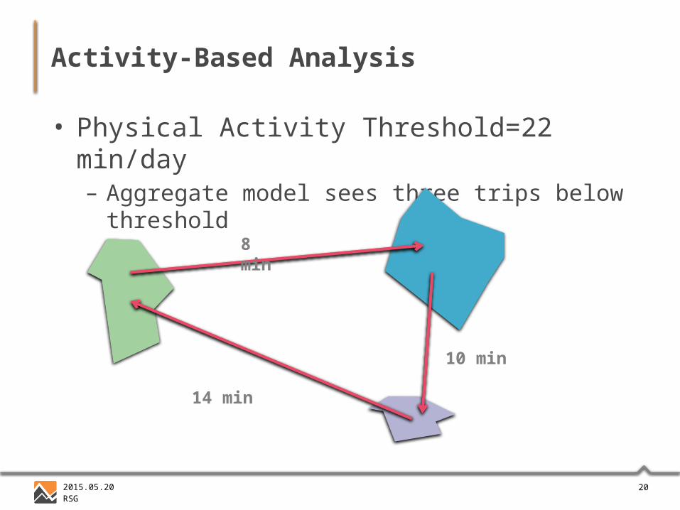
Activity-Based Analysis
• Physical Activity Threshold=22 min/day– Aggregate model sees three trips below threshold
8 min
10 min
14 min
212015.05.20RSG
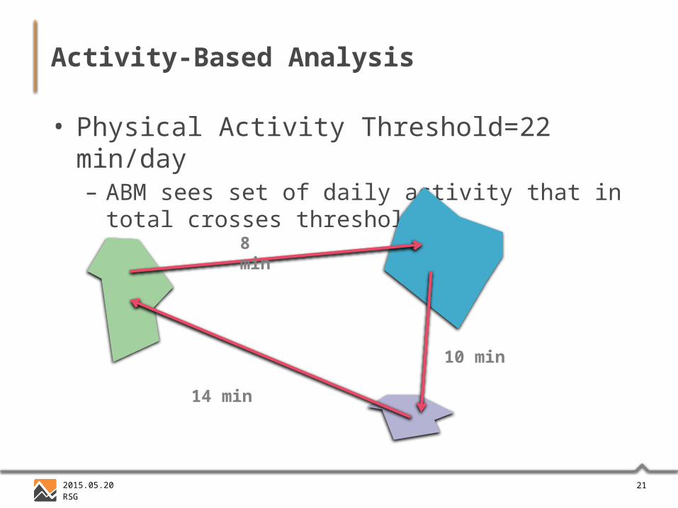
Activity-Based Analysis
• Physical Activity Threshold=22 min/day– ABM sees set of daily activity that in total crosses
threshold
8 min
10 min
14 min
222015.05.20RSG
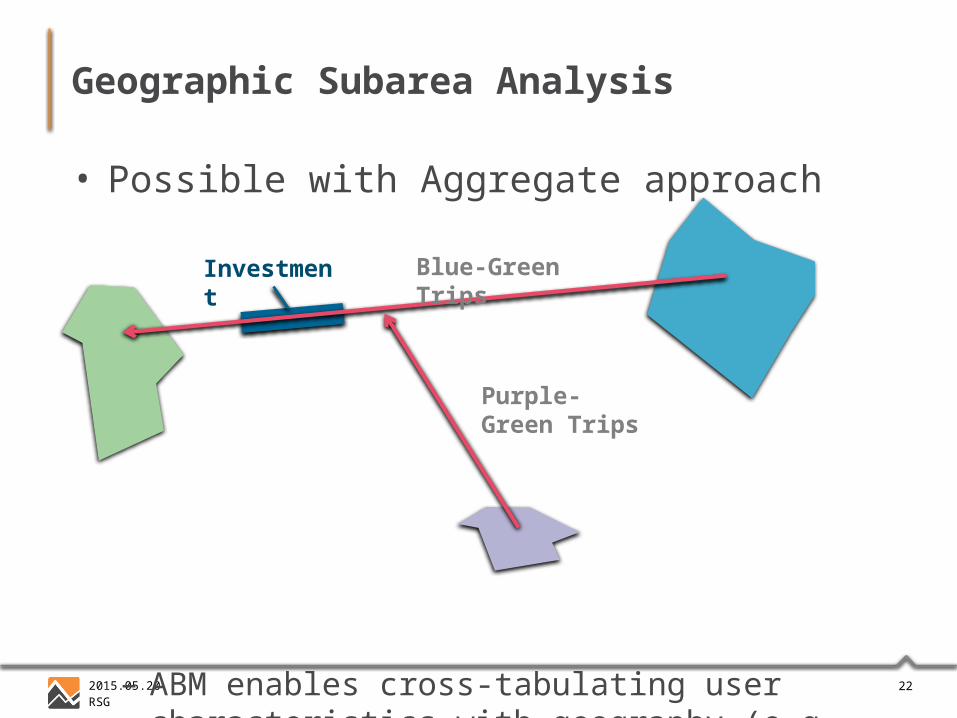
Geographic Subarea Analysis
• Possible with Aggregate approach
– ABM enables cross-tabulating user characteristics with geography (e.g. Blue-Green Trips by EJ folks)
Investment
Purple-Green Trips
Blue-Green Trips
232015.05.20RSG
Challenges
Imputation of transit impedances when not present in base or scenario alternative Segmented by access type Based on drive alone auto distances
Different resolutions Disaggregate trips Persons Links OD pairs
Limitations of COC benefit segmentation
242015.05.20RSG
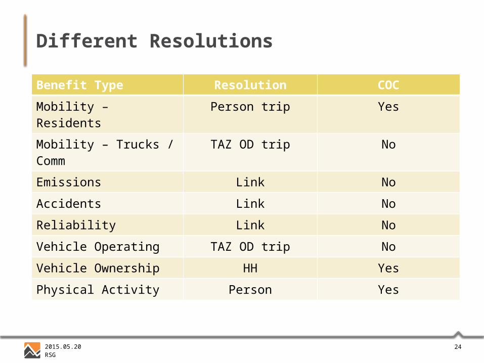
Different Resolutions
Benefit Type Resolution COC
Mobility – Residents Person trip Yes
Mobility – Trucks / Comm TAZ OD trip No
Emissions Link No
Accidents Link No
Reliability Link No
Vehicle Operating TAZ OD trip No
Vehicle Ownership HH Yes
Physical Activity Person Yes
252015.05.20RSG
Future Developments
Extension of COC reporting Emissions Accidents Reliability Vehicle Operating
Improved user interface Flexible COC specification Performance Tuning
262015.05.20RSG
Sources for Valuation and How-To
Travel Demand Forecasting Value-of-Time Definition Implied VOT: ratio of time and cost coefficients in the (primary) mode
choice statistical model
USDOT Value-of-Time Definition USDOT. The Value of Travel Time Savings: Departmental Guidance
for Conducting Economic Evaluations Revision 2. 2011.
AASHTO “Red Book” (project-level BCA) American Association of State Highway and Transportation Officials.
User and Non-User Benefit Analysis for Highways. 2010
272015.05.20RSG
Thank You!
Joe Castiglione617.251.5111
Jeff Frkonja312.605.9213
619.699.7325

Reserve Slides
292015.05.20RSG
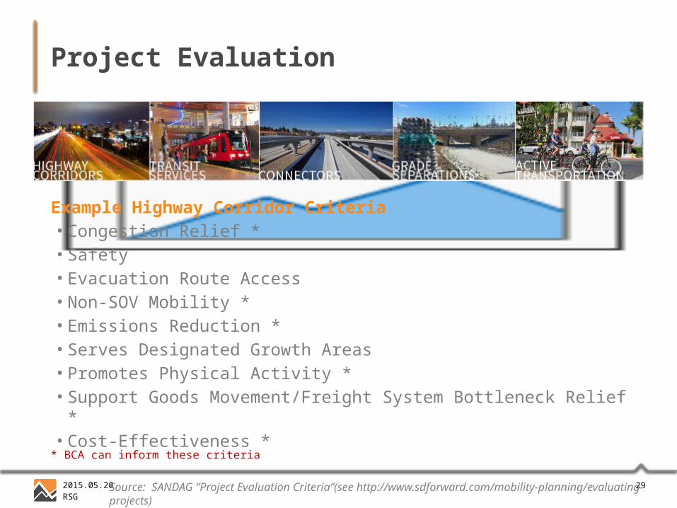
Project Evaluation
Click to add photo
Example Highway Corridor Criteria• Congestion Relief *• Safety• Evacuation Route Access• Non-SOV Mobility *• Emissions Reduction *• Serves Designated Growth Areas• Promotes Physical Activity *• Support Goods Movement/Freight System Bottleneck Relief *• Cost-Effectiveness *
Source: SANDAG “Project Evaluation Criteria”(see http://www.sdforward.com/mobility-planning/evaluating-projects)
* BCA can inform these criteria
302015.05.20RSG
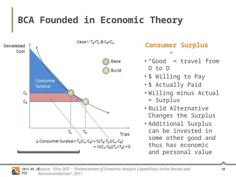
BCA Founded in Economic Theory
Consumer Surplus
• “Good” = travel from O to D• $ Willing to Pay• $ Actually Paid• Willing minus Actual =
Surplus• Build Alternative Changes
the Surplus• Additional Surplus can be
invested in some other good and thus has economic and personal value
Click to add photo
Source: Ohio DOT : “Enhancement of Economic Analysis Capabilities: Initial Review and Recommendations”. 2011
312015.05.20RSG
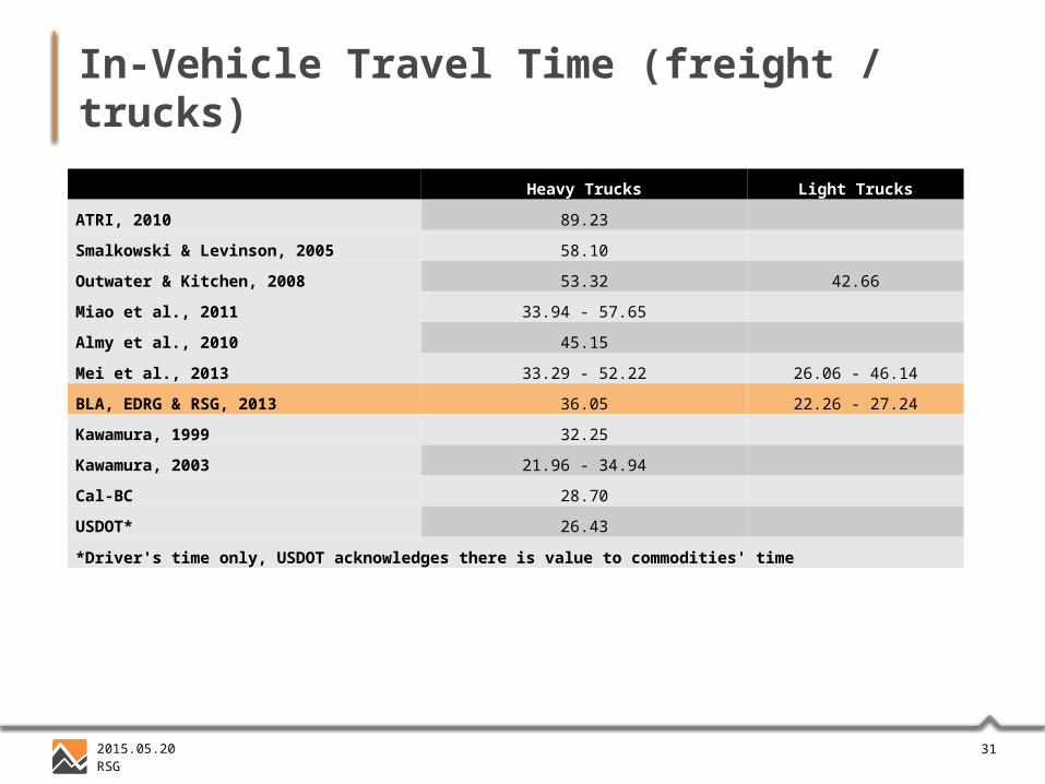
In-Vehicle Travel Time (freight / trucks)
Heavy Trucks Light Trucks
ATRI, 2010 89.23
Smalkowski & Levinson, 2005 58.10
Outwater & Kitchen, 2008 53.32 42.66
Miao et al., 2011 33.94 - 57.65
Almy et al., 2010 45.15
Mei et al., 2013 33.29 - 52.22 26.06 - 46.14
BLA, EDRG & RSG, 2013 36.05 22.26 - 27.24
Kawamura, 1999 32.25
Kawamura, 2003 21.96 - 34.94
Cal-BC 28.70
USDOT* 26.43
*Driver's time only, USDOT acknowledges there is value to commodities' time
322015.05.20RSG
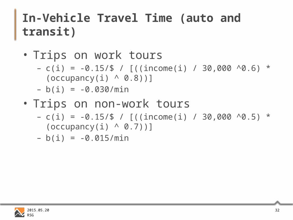
In-Vehicle Travel Time (auto and transit)
• Trips on work tours– c(i) = -0.15/$ / [((income(i) / 30,000 ^0.6) * (occupancy(i) ^
0.8))]– b(i) = -0.030/min
• Trips on non-work tours– c(i) = -0.15/$ / [((income(i) / 30,000 ^0.5) * (occupancy(i) ^
0.7))]– b(i) = -0.015/min
332015.05.20RSG
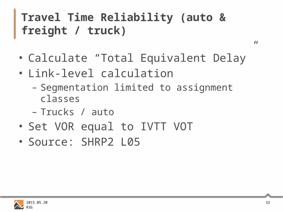
Travel Time Reliability (auto & freight / truck)
• Calculate “Total Equivalent Delay”• Link-level calculation
– Segmentation limited to assignment classes– Trucks / auto
• Set VOR equal to IVTT VOT• Source: SHRP2 L05
342015.05.20RSG
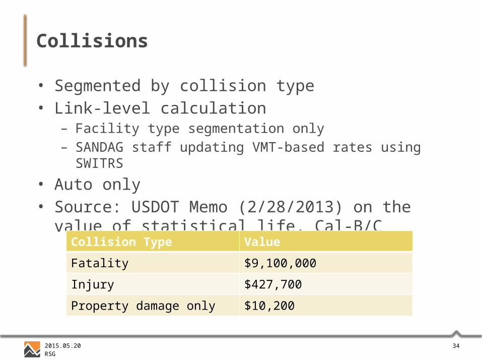
Collisions
• Segmented by collision type• Link-level calculation
– Facility type segmentation only– SANDAG staff updating VMT-based rates using SWITRS
• Auto only• Source: USDOT Memo (2/28/2013) on the value of
statistical life, Cal-B/C
Collision Type Value
Fatality $9,100,000
Injury $427,700
Property damage only $10,200
352015.05.20RSG
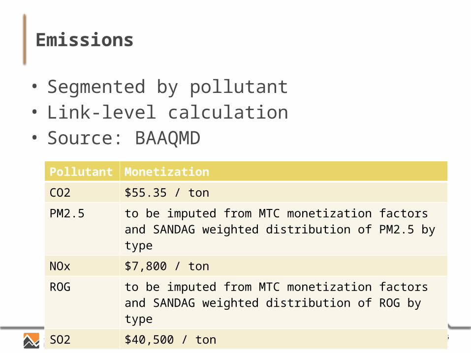
Emissions
• Segmented by pollutant• Link-level calculation• Source: BAAQMD
Pollutant Monetization
CO2 $55.35 / ton
PM2.5 to be imputed from MTC monetization factors and SANDAG weighted distribution of PM2.5 by type
NOx $7,800 / ton
ROG to be imputed from MTC monetization factors and SANDAG weighted distribution of ROG by type
SO2 $40,500 / ton
362015.05.20RSG
Auto Ownership Costs
• MTC = $6,290 / year• AAA = $6,000 / year• Household-level calculation• Source: MTC