Benchmarking of Israeli economic time series and seasonal

Benchmarking of Israeli economic time series and seasonal adjustment

ISSN 1725-4825

E U R O P E A NC O M M I S S I O NW

OR

KI

NG

P

AP

ER

S

AN

D

ST

UD

IE

S

ED

ITIO

N2

00

5

A great deal of additional information on the European Union is available on the Internet.It can be accessed through the Europa server (http://europa.eu.int).

Luxembourg: Office for Official Publications of the European Communities, 2005

© European Communities, 2005

Europe Direct is a service to help you find answers to your questions about the European Union

New freephone number:

00 800 6 7 8 9 10 11

ISSN 1725-4825ISBN 92-79-01317-3

Statistical Analysis Division

Benchmarking of Israeli Economic Time Series

and Seasonal Adjustment

Yury Gubman and Luisa Burck Central Bureau of Statistics, Israel

March, 2005

Abstract Benchmarking deals with the problem of combining a series of high-frequency data (e.g., monthly) with a series of low frequency data (e.g., quarterly) into a consistent time series. When discrepancies arise between the two series the latter is usually assumed to provide more reliable information. There are two main approaches to benchmarking of time series: a purely numerical approach and a statistical modeling approach. The numerical approach encompasses the family of least-square minimization methods (Denton, 1971). This benchmarking procedure is based on a movement preservation principle that is widely used by government statistical agencies and central banks around the world. Statistical modeling approaches include ARIMA-based methods proposed by Hillmer and Trabelsi (1987, 1990), regression models (Cholette and Dagum, 1991), state space models (Durbin and Quenneville, 1997). At the Central Bureau of Statistics (CBS) Israel, the need for the application of benchmarking techniques arises, for example for Labour Force Survey data and for National Accounts estimates, where monthly or quarterly and quarterly or annual data, respectively, may show inconsistent movements. Generally, the binding benchmarking technique seems to be the most appropriate for a statistical agency for solving the problem of discrepancies in the original administrative data, and the unbinding methods may be useful for survey data with known standard deviation. However, since these series are seasonally adjusted anew each month (quarter) several problems may arise because of the filtering process. Furthermore, when a system of time series is seasonally adjusted, the accounting constraints that link the original series may no longer be fulfilled. In this paper, an empirical study that compares between the Denton approach and the regression approach is carried out for several Labour Force series, when a special emphasis is put on issues concerning seasonal adjustment: seasonal pattern preservation and the quality of the seasonal adjustment. In addition, the seasonal adjustment and the benchmarking of the composite series are considered when dealing with a system of time series. The indirect benchmarking method is proposed for benchmarking the composite and the component series. The statistical quality issues related to the benchmarking procedure and seasonal adjustment are discussed.

Keywords: Benchmarking methods, Denton’s movement preservation method, Regression approach, Seasonal adjustment, Statistical data quality.

2

1. Introduction

Benchmarking is an important problem faced by the statistical agencies. For a target

socioeconomic variable, two sources of data, for example, an annual administrative

data and a quarterly repeated survey data, may be available. When discrepancies

between the series of high frequency (e.g. quarterly) data and a series of low

frequency (e.g. annual) data arise the latter is usually assumed to provide more

reliable information. The problem of adjusting the monthly or quarterly time series to

make them consistent with the quarterly or annual totals is known as benchmarking.

There are two main approaches to benchmarking of time series: a purely numerical

approach and a statistical approach. The first includes the family of least-square

minimization methods and is based on a movement preservation principle (Denton,

1971). The latter includes ARIMA-based signal extraction method (Hillmer and

Trabelsi, 1987, 1990), regression models (Cholette and Dagum, 1994) and state-space

models (Durbin and Quenneville, 1997).

Formally, let be the series of high frequency: tY

ttt eY +=θ , Tt ,...,1= , (1)

and be the stock series of low frequency: mZ

mmt

tm

m wp

Z += ∑∈

θ1 , Mm ,...,1= , (2)

where and are the respective survey errors and te mw mt ∈ means that t is included

in the time period covered by , and is the number of high-frequency

observations covered by . For stock series

mZ mp

mZ mpm ∀≡ ,1 .

Forcing monthly or quarterly figures to be equal to the given quarterly or annual totals

(benchmark), leads to the binding benchmarking technique that seems to be the most

appropriate for certain series, e.g. the national accounts series, published by the

statistical agency. By setting mwm ∀= ,0 , in (2) the binding benchmarking is

realized and the high-frequency time series is revised under the assumption that the

low-frequency data is "true" in terms of survey errors. Otherwise, the benchmarking is

unbinding. In this case one can adjust the original high-frequency data using the

external data (e.g. quarterly or annual totals), under some accounting constrains, but

without forcing the sums to match exactly the low-frequency data of the relevant time

3

period. The main advantage of this method is that it exploits the additional

information about the autocorrelation structure of the benchmarks. As a result, the

estimation errors from the unbinding benchmarking techniques usually are smaller.

The unbinding technique may be applied to survey data, for which the assumption

about zero variance of benchmark series is too strong.

At the Central Bureau of Statistics (CBS), Israel, the need for the application of

benchmarking techniques arises, mainly, for Labour Force Survey Data and for

National Accounts estimates, where monthly or quarterly and quarterly or annual

data, respectively, may show inconsistent movements. However, several problems in

seasonal adjustment and in benchmarking of the systems of time series may arise

because of the filtering process.

At the CBS, seasonal adjustment is carried out using the X-12-ARIMA program that

was developed by the US Census, 1998. This method is based on moving averages

filtering process for the estimation of seasonal and trend-cycle components of time

series. Two main problems in benchmarking procedure arise using this method:

1. The concurrent seasonal adjustment process in use at the CBS introduces

revisions in the seasonally adjusted series and the trend-cycle estimates, since

these series are seasonally adjusted anew each month or quarter.

Benchmarking procedure also causes revisions in the original data, and

together with the seasonal adjustment procedure they may increase the size of

these revisions. As a result, the seasonal pattern of the series might be affected

due to these revisions.

2. When a system of time series is seasonally adjusted, the accounting constraints

that link the original series may no longer be fulfilled. Applying benchmarking

process, which also affects these links, may increase the size of the

discrepancies.

In this paper, the Labour Force Survey data is analyzed. The Israel Labour Force

Survey is carried out by the CBS and serves as a source of data on the labour force

characteristics and trends as well as household economics and demographics. The

survey is designed as an annual survey of a nationally representative sample of

approximately 12,000 households, and about 23,000 different households are

interviewed every year. The survey population includes the whole permanent

population of Israel aged 15 and over. The rotation panel structure of the survey

provides repeated measurements on the same sample at different time points during

4

18 months and leads to 50% overlap between two consecutive quarters. This enables

estimation of gross changes between the quarters. The CBS also produces very

limited monthly data on labour force characteristics; mainly, number of employed and

unemployed persons, by sex.

The empirical study focuses on issues concerning with seasonal adjustment and a

special emphasis is put on data quality issues. Revisions in the seasonally adjusted

series before and after benchmarking and the seasonal patterns of the original and the

benchmarked series for several benchmarking techniques are studied. The direct and

indirect benchmarking methods of a system of time series are compared, similarly to

direct and indirect seasonal adjustment methods that are well known. Several

accounting links preservation methods are examined, and a solution for the method

based on the regression approach is provided.

2. Benchmarking methods

As stated above, several approaches exist to the benchmarking problem. In this

section two main benchmarking methods that are relevant to the official statistics are

reviewed. Let us point out that other benchmarking methods were developed, such as

state space model (Pfefferman and Burck, 1990, Durbin and Quenneville, 1997) and

models based on small area estimation (Pfefferman , 2002, Pfefferman and Tiller,

2003).

2.1. Denton's benchmarking method

The Denton family of least-squares based benchmarking methods is widely used by

statistical agencies and international institutes around the world to solve the

benchmarking problem (IMF, 2002). The general objective of this technique is a)

maximum preservation of the short-term movements in the original (indicator) series

and b) to obtain exact benchmark to total (binding). The estimation of a benchmarked

series is based upon the minimization of a penalty function subject to a given set of

benchmarking constrains. Let ),( λθL be Lagrangian function:

(3) )()()(),( '' θλθθλθ LZYAYL −+−−=

where Y denotes the original series,θ defines the benchmarked series to be estimated,

5

Z is the low-frequency benchmarks, L is a design matrix that defines the links

between the original series and the benchmarks, and A is a matrix used to define the

special objective function. The solution for (3) is provided by:

)()( ''^

LYZLLALAY −+= −−− 111θ (4)

The two main variants of Denton’s benchmarking procedure are:

1. The additive method that preserves the simple period-to-period change:

TtMmmtYYYY tttttttt ,...,1,,...,1,),()()()( 1111 ==∈−−−≡−−− −−−− θθθθ

The objective function to be minimized for the first differences is thus given

by:

211

2)]()[(min −−

=

−−−∑ tt

T

ttt YY θθ

θ (5)

2. The proportional method that preserves the proportional period-to-period

change:

TtMmmtYYYY

t

t

t

t

t

tt

t

tt ,...,1,,...,1,,1

1

1

11 ==∈−≡−

−−

−

−

−

−−

θθθθ

θθ

The objective function to be minimized for the first differences is thus given

by:

2

1

1

2

)]()[(min−

−

=

−∑t

tT

t t

t YYθθθ

(6)

One can think about other forms of the objective functions, as it has been shown by

Denton (1971), Helfand, Monsour and Trager (1977), Fernandez (1981) and Cholette

(1979, 1984). Generally, the Denton technique is relatively simple, robust and well

suited for large-scale applications. Moreover, the proportional method provides an

effective framework for benchmarking, interpolation and extrapolation of time series

that preserves month-to-month (quarter-to-quarter) changes in the data. On the other

hand, these methods do not use any additional information in the data, such as

correlation structure of the series or the survey errors.

2.2. Regression approach

The stochastic approach to benchmarking problem proposed by Hillmer and Trabelsi

(1987, 1990) is well known as signal extraction method and it assumes that a signal θ

follows an ARIMA model. A more general regression approach was developed by

6

Cholette and Dagum (1994) and is implemented the BENCH program written by the

Canadian staff (1994). The model consists of two linear equations:

MmwEwEwpZ

TteeEeEeaY

m

ktt

wmmmt

mmtm

keektttttt

,...,1,)(,0)(,/)(

,...,1,)(,0)(,22 ===+=

===++=

∑∈

− −

σθ

ρσσθ (7)

The equations (7) define the additive benchmarking model, where a is constant bias

(intercept), and are the autocorrelated errors that may be interpreted as survey

errors. These errors may be heteroscedastic, i.e. the variance may vary with time

t. The autocorrelations

te

2teσ

kρ correspond to those of a stationary and invertible Auto

Regressive Moving Average (ARMA) process, supplied by the user. This is

equivalent to assuming that follows a process given by: te

ttte εσ= ,

where tε follows the selected stationary ARMA process:

tqtp vBB )()( ηεφ = ,

where B is the backshift operator, )(Bpφ and )(Bqη are the autoregressive (AR) and

moving average (MA) polynomials respectively and is white noise. tv

Replacing the first equation in (7) by:

tttttt eaeaY lnlnln)ln(ln ++=××= θθ (7a)

leads to the multiplicative (log-additive) model, and if this model is replaced by:

ttt eaY +×= θ (7b)

the mixed benchmarking model is obtained. The GLS solution for all these models

are given in Cholette and Dagum (1994). The binding regression method is achieved

by setting . It may be shown that either additive or multiplicative

Denton technique is a special case of the regression method under the following

assumptions:

mwm ∀= ,0

1. follows the random walk process; te

2. , i.e. the benchmarking is binding; mwm ∀= ,0

3. variances of high-frequency data are constant; tY

4. bias parameter a is omitted.

7

Under these assumptions the additive regression model corresponds to the additive

Denton method and the multiplicative regression model corresponds to the

proportional Denton method.

Cholette and Dagum (1994) showed that the regression framework provides BLUE

estimates. Also, the method has several desirable features: it allows to adjust all types

of time series, it takes into account a stochastic structure of the series, it preserves

movements of the original series, minimizes revisions in the data, and some other.

When the binding possibility may be preferable for the national account series with an

administrative indicator series of benchmarks, the unbinding regression method may

be useful for survey data for which the assumption of zero variance of the low-

frequency data may be unreasonable.

3. Issues on Seasonal Adjustment

3.1. Seasonal Adjustment in CBS

More then 400 monthly and quarterly time series are seasonally adjusted at the CBS.

The time series collected by the CBS are statistical records of a particular social or

economic activity, like industrial production, person-nights in tourist hotels, labour

force characteristics. They are measured at regular intervals of time, usually monthly

or quarterly, over relatively long periods. This allows to disclose patterns of behavior

over time, to analyze them and place the current estimates into a more meaningful

and historical perspective. All the series are seasonally adjusted by the X-12-ARIMA

program, which became the standard program for seasonal adjustment in 2004.

A time series can be decomposed into a number of fundamental components, each of

which has its own distinguishing character. In a simple model, the original data at any

time point (denoted by ) may be expressed as a function of three main

components: the seasonality ( ), the trend-cycle ( ), and the irregularity ( ), that

is:

tO f

tS tC tI

),,( tttt ICSfO = . (8)

8

Depending mainly on the nature of the seasonal movements of a given series, several

different models can be used to describe the way in which the components , ,

and are combined to compose the original series . The multiplicative model:

tC tS

tI tO

tttt ICSO ××=

treats all three components as dependent of each other; that is, the seasonal oscillation

size increases and decreases with the level of the series. The irregular factors may

be decomposed into sub-components: the changes in the number of trading days and

festival dates (also called calendar effects), and the remaining irregularity. Therefore

the model may be extended as follows:

tI

ttt EPI ×=

and thus:

ttttt EPSCO ×××=

where, is the adjustment factor for the calendar effects (changes in the festival

dates and the number of trading days in a month) and is the residual variation

caused by all other influences. Most series at the CBS, including National Accounts

and Labour Force Survey series, are adjusted multiplicatively.

tP

tE

3.2. Concurrent Seasonal Adjustment

Concurrent Seasonal Adjustment means that the seasonal adjusted series is calculated

anew each month (quarter) on the basis of data that includes the current (new)

observation. In general, new data contribute new information about changes in the

seasonal pattern that preferably should be incorporated as early as possible. When

concurrent seasonal adjustment is applied to a series, the seasonally adjusted values

for the whole series, including the most recent month (quarter), are obtained directly

from the seasonal adjustment procedure without the use of forecast seasonal and prior

adjustment factors. Empirical studies have shown that the revisions to the seasonally

adjusted data are smaller for series seasonally adjusted using the concurrent method.

Concurrent seasonal adjustment is applied to all series published in the Monthly

Bulletin of Statistics and in other publications of the CBS.

9

3.3. Seasonal Adjustment of Composite Time Series

An aggregate (composite) series is a series that is composed of several sub-series

(components). The direct seasonal adjustment method means seasonally adjusting the

composite and the component series independently. Whereas, the indirect seasonal

adjustment method consists of seasonally adjusting each component series and then

obtaining the seasonally adjusted composite series as their sum.

The advantage of the indirect method is that the changes in the composite series can

be broken down into the changes of the component series. Those component series

for which the relative contribution of seasonality is low and/or the contribution of the

irregular component is high, are included in the sum as unadjusted series. The

monthly labour force series are adjusted using the indirect method.

4. Benchmarking and Seasonal Adjustment – Problems

Benchmarking of the original time series may introduce several problems in seasonal

adjustment process.

4.1. Single series

a) The seasonal factors, which are estimated from the decomposition model (8)

by the filtering process, may change by pre-adjusting the series to benchmark

values. Benchmarking procedure may cause a significant increase in the

variance of the irregular component of the original time series if outliers exist

in the benchmark series. In the case of benchmarking of the monthly series by

quarterly benchmarks, revisions in seasonal pattern of the series may be

caused by seasonal and irregular fluctuations in the quarterly data. These

changes may affect the estimation of seasonal factors and, thus, seasonally

adjusted series. All these changes are undesirable and in this case a

benchmarking model that preserves the seasonal pattern of the original data is

preferable to others.

b) In general, since the benchmarking may affect the irregular component of a

time series, the trading day and holiday effects ( ) estimation may also be

affected. In this paper the impact of benchmarking on this estimation is not

tP

10

investigated, but still it must be pointed out that in a series with significant

trading day and holiday influences, large changes in the irregular component

may seriously affect the estimation of . tP

c) The estimated seasonal factors and seasonally adjusted series are subject to

revisions every month or quarter under concurrent seasonal adjustment

method. Since this method is applied to all series published by the CBS, the

benchmarking revisions become more critical. Large revisions in the original

data each month (quarter) due to computational processes are a problem, and

we would prefer a benchmarking method with relatively small size of

revisions.

4.2. Composite series

a) Applying the seasonal adjustment procedure to a system of time series, where

a number of sub-series are summed up to form the aggregate (composite)

series, breaks off the links and the accounting constraints are no more fulfilled.

On the other hand, applying the benchmarking procedure directly to the sub-

series and to the grand-total series also violates these constraints. As was

pointed out in section 3.3, the indirect seasonal adjustment method

successfully avoids this danger without affecting, in many cases, the quality of

the seasonally adjusted series. The same principle may be applied to the

benchmarking: it is trivial that if all sub-series are benchmarked directly and

the composite series obtained by summing them up will also be benchmarked.

Consequently, one has to develop the criteria for selecting the indirect and the

direct benchmarking methods for a specific system of time series.

b) When the indirect procedure cannot be applied due to statistical or

econometrical reasons to a system of time series, the account links

preservation problem arises. Di Fonzo and Marini (2003) proposed a

benchmarking method for adjusting a system of seasonally adjusted time

series, using the Denton technique. If another benchmarking method seems to

be appropriate, a more general approach must be developed.

4.2.1. Methods for preservation of accounting links

11

Here we summarize several approaches that preserve the accounting links in

benchmarking and propose a technique based on the regression principle. The indirect

benchmarking method preserves the accounting links between sub-series and

composite series. An empirical analysis that compares direct to the indirect

benchmarking is presented in section 5.3. The indirect benchmarking method is

consistent with indirect seasonal adjustment in terms of seasonal pattern preservation

in the sub-series, where the seasonal fluctuations in the sub-series are not swallowed

up in the composite data.

If, for some reason, the direct adjustment is applied to all series in the system, the

accounting constraints that linked the original series will be violated after

benchmarking procedure. Several methods are considered in order to overcome this

type of problem. First, one can simply divide amongst the sub-series the difference

between the sum of the benchmarked sub-series and benchmarked aggregate series,

for example, by the weights of the sub-series. This intuitive approach may be useful in

some cases, for example, in benchmarking of two different systems of time series

when the aggregate data has two different breakdowns. An example of this in the CBS

is the composite monthly series of employed persons, by sex and by economic branch.

For monthly employed males and females and for their totals we have quarterly

benchmarks, but we have no additional information about the latter set of series. The

proposed algorithm that preserves the accounting links for these series is as follows:

a) Apply the benchmarking procedure that preserves the accounting links to the

first system (i.e. employed persons by sex) to obtain the benchmarked

composite series (for example, by applying indirect method).

b) Calculate the difference between the benchmarked composite series and the

sum of the sub-series from the second system.

c) Add to each sub-series the relative difference, based on the weight of the sub-

series in the aggregate figure. Calculating weights for each observation rather

than using the average weight value for all observations will cause smaller

revisions and better preservation of month-to-month rates of change in the

sub-series.

This very simple technique may also be useful in adjustment of single system of time

series, when the benchmark values are available only for the composite data.

Obviously, we need a more sophisticated approach for the case when benchmarks are

available for all series and direct benchmarking technique seems to be appropriate. Di

12

Fonzo and Marini (2003) presented accounting link preservation method based on

Denton approach. We propose here a more general approach based on the regression

principle to preserve the accounting links between the sub-series.

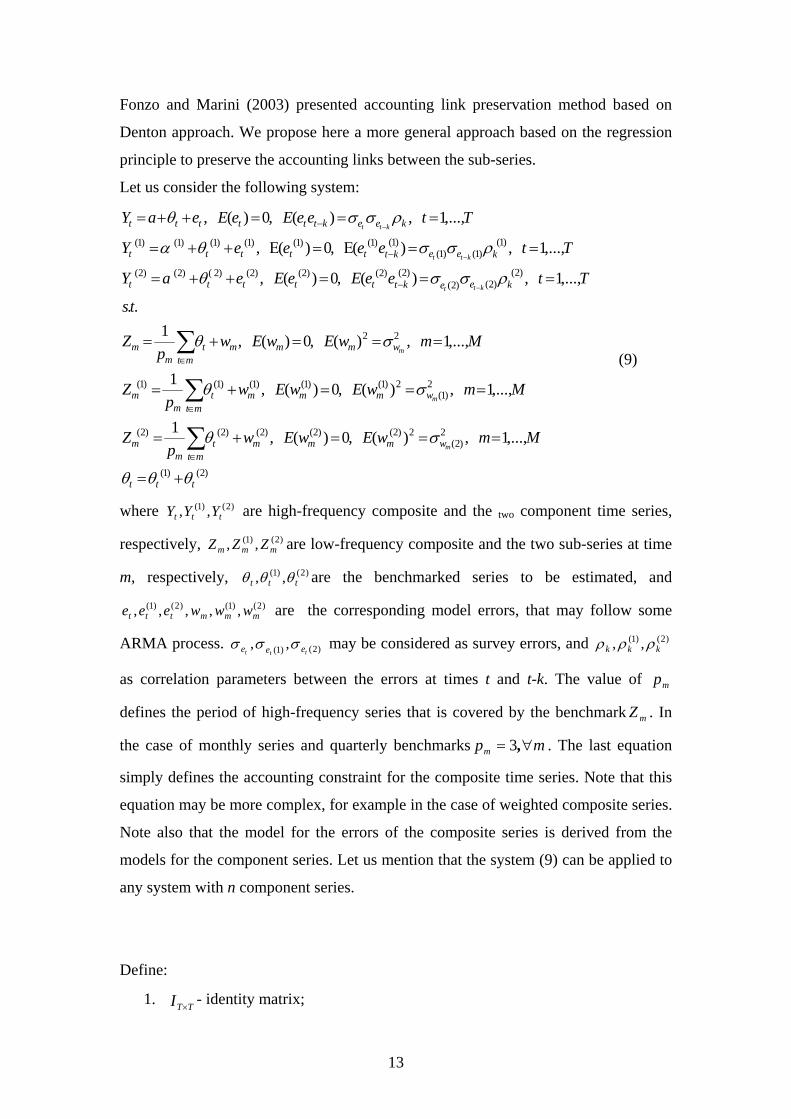
Let us consider the following system:

)2()1(

2)2(

2)2()2()2()2()2(

2)1(

2)1()1()1()1()1(

22

)2()2()2(

)2()2()2()2()2()2()2(

)1()1()1(

)1()1()1()1()1()1()1(

,...,1,)(,0)(,1

,...,1,)(,0)(,1

,...,1,)(,0)(,1..

,...,1,)(,0)(,

,...,1,)(,0)(,

,...,1,)(,0)(,

ttt

wmmmmt

tm

m

wmmmmt

tm

m

wmmmmt

tm

m

keektttttt

keektttttt

keektttttt

MmwEwEwp

Z

MmwEwEwp

Z

MmwEwEwp

Z

ts

TteeEeEeaY

TteeeeY

TteeEeEeaY

m

m

m

ktt

ktt

ktt

θθθ

σθ

σθ

σθ

ρσσθ

ρσσθα

ρσσθ

+=

===+=

===+=

===+=

===++=

==Ε=Ε++=

===++=

∑

∑

∑

∈

∈

∈

−

−

−

−

−

−

(9)

where are high-frequency composite and the )2()1( ,, ttt YYY two component time series,

respectively, are low-frequency composite and the two sub-series at time

m, respectively, are the benchmarked series to be estimated, and

are the corresponding model errors, that may follow some

ARMA process. may be considered as survey errors, and

as correlation parameters between the errors at times t and t-k. The value of

defines the period of high-frequency series that is covered by the benchmark . In

the case of monthly series and quarterly benchmarks

)2()1( ,, mmm ZZZ

)2()1( ,, ttt θθθ

)2()1()2()1( ,,,,, mmmttt wwweee

)2()1( ,,ttt eee σσσ )2()1( ,, kkk ρρρ

mp

mZ

mpm ∀= ,3 . The last equation

simply defines the accounting constraint for the composite time series. Note that this

equation may be more complex, for example in the case of weighted composite series.

Note also that the model for the errors of the composite series is derived from the

models for the component series. Let us mention that the system (9) can be applied to

any system with n component series.

Define:

1. - identity matrix; TTI ×

13

2. - matrix in which: TMJ ×⎪⎭

⎪⎬⎫

⎪⎩

⎪⎨⎧

∉

∈=×

mt

mtpJ mtm,

,

0

1

3. - vector of ones. tu

We can rewrite the model in (9) in the matrix notation as follows:

vXY += β* (10)

where:

1)33()2(

)1(

)2(

)1(

*

×+⎥⎥⎥⎥⎥⎥⎥⎥

⎦

⎤

⎢⎢⎢⎢⎢⎢⎢⎢

⎣

⎡

=

MTZ

Z

ZY

Y

Y

Y ,

1)33()2(

)1(

)2(

)1(

×+⎥⎥⎥⎥⎥⎥⎥⎥

⎦

⎤

⎢⎢⎢⎢⎢⎢⎢⎢

⎣

⎡

=

MTw

w

we

e

e

v ,

1)32()2(

)1(

)2(

)1(

×+⎥⎥⎥⎥⎥⎥⎥

⎦

⎤

⎢⎢⎢⎢⎢⎢⎢

⎣

⎡

=

T

a

a

a

θ

θ

β

with the design matrix X:

)32()33(00000000

000000

00000

+××⎥⎥⎥⎥⎥⎥⎥⎥

⎦

⎤

⎢⎢⎢⎢⎢⎢⎢⎢

⎣

⎡

=

TMTJJ

JJIu

IuIIu

X

The correlation structure is defined by:

)33()33(0

0)'(,0)(

MTMT

e

WV

VVvvEvE

+×+

⎥⎦

⎤⎢⎣

⎡===

where and are the covariance matrices for the high-frequency and the low-

frequency series, respectively. Note that X and V matrix are of full rank. The General

Least Square estimates of the model parameters (10) are given by:

eV wV

11'^

*1'11^

)()(

)'(

−−

−−−

=

=

XVXCov

YVXXVX

β

β

Simplification of this expression is possible in order to decrease the dimension, of this

problem, as shown by Cholette and Dagum (1994). It was also shown that the above

estimates are BLUE. The estimation of the multiplicative and mixed regression

models can be carried out by applying the same principles as in the additive case after

some transformation (log-transformation for the multiplicative case), as shown by the

14

Canadian Staff (1994). Denton benchmarking procedure is equivalent when the

following settings are applied:

1. follow the random walk model, )2()1(, , ttt eee

2. intercepts a, a(1), a(2) are omitted,

3. benchmarking is binding, i.e. 0,, )2()1( ≡mmm www

4. appropriate regression model is chosen (additive for Denton additive method and

multiplicative for Denton proportional method).

5. Empirical study

The empirical study presented here includes a comparison between several

benchmarking models for the labour force series and it focuses on seasonal

adjustment. The requirement from the benchmarking model is such that it does not

cause, as much as possible, distortion of the seasonal pattern of the series, and does

not significantly affect the irregular movements. Note that all benchmarking

calculations were carried out by the BENCH program (Canadian Staff, 1994), and the

seasonal adjustment figures were obtained using the X-12-ARIMA program (US

Census, 1998).

5.1. Benchmarking models and Seasonal Adjustment

In the following, we examine five binding and three unbinding benchmarking

methods:

1) Denton additive model (5).

2) Denton proportional model (6).

3) Binding, i.e. , regression additive model (7), with ARMA

model for .

mwm ∀= ,0

te

4) Binding, i.e. , regression multiplicative model (7a), with

ARMA model for .

mwm ∀= ,0

te

5) Binding, i.e. , regression mixed model (7b), with ARMA

model for .

mwm ∀= ,0

te

6) Unbinding regression additive model (7), with ARMA model for . te

15

7) Unbinding regression multiplicative model (7a), with ARMA model

for . te

8) Unbinding regression mixed model (7b), with ARMA model for . te

For each model, the benchmarking procedure is applied to the original data, and then

the seasonal adjustment program is executed. Note that the ARMA model is estimated

from the irregular part of the time series. Four monthly labour force sub-series are

analyzed: employed males, employed females, unemployed males, and unemployed

females. Direct and indirect benchmarking and seasonal adjustment methods are

compared for the composite series, Total unemployed persons.

5.2. Statistics for model comparison

5.2.1. Benchmarking statistics

The ARMA model for the errors and the parameter values are estimated, for all

relevant time series. Three main statistics are calculated for the benchmarked series:

te

1) Average standard deviation = ∑=

T

ttstd

T 1

^)(1 θ

2) Movement preservation statistic, in percentages, defined by:

M= 100*][1

1

2 1^

^

1∑= −−

−−

T

t t

t

t

t

YY

absT θ

θ .

This statistic is calculated as the average of differences, in absolute values,

between the month-to-month rate of change in the original and the

benchmarked series. The value of M will be smaller for the model that

preserves better the month-to-month rate of change.

3) Range of seasonality preservation. The difference between the highest (peak)

and the lowest (trough) of the annual seasonal factors, expressed in

percentages, is called the range of seasonality, and is a measure of the

magnitude of the seasonal variation. Denote seasonal factors by : tS

)(min)(max12,...,112,...,1 tttt

SSyseasonalitofRangeR==

−== .

Using the range of seasonality, the Israeli series were classified into three

groups: a) high seasonality (range greater than 50 %), b) intermediate (20-50

%), and c) low (less than 20 %). Note, that unemployed females series is of

intermediate seasonality, and all other series are of low seasonality.

16

The important property of the benchmarking method is to preserve the range

of seasonality of time series. Thus, we introduce the following statistic for

preservation of range of seasonality:

DR=R of original series – R of benchmarked time series.

Thus, a smaller value of DR means a similar range of seasonality in the

benchmarked series.

5.2.2. Seasonal adjustment statistics

The X-12-ARIMA program produces a set of standard statistics for fitting the

ARIMA model and for the quality of the seasonal adjustment; all these statistics are

described in the X-12-ARIMA manual and in Findley (1998). In this paper, we refer

to several statistics that are widely used at the CBS when we apply the seasonal

adjustment procedure to a specific series.

1) ARIMA model statistics: model coefficients and their significance, average

absolute percentage error in within sample forecasts for last three years, Chi-

Square probability for goodness of fit, normality of the residuals, and log-

likelihood based statistics.

2) Seasonal adjustment statistics: F test for stable seasonality (table D8A),

standard deviation of estimated seasonal factors (table D10) and irregular

factors (table D13), relative contributions in percentages of the components to

the variance in the month-to-month changes in the original series (table F2B),

number of months for cyclical dominance MCD (table F2E), and quality

assessment summary statistic Q (table F3).

A new measurement was added: smoothness of the seasonally adjusted series, in

percentages, defined by:

Smoothness= 100*)]1[(1

1

2 1∑= −

−−

T

t t

t

YY

absT

The smoothness index is computed as the average of the absolute percent month-to-

month change in the series.

5.3. Empirical Results

Table 1 to Table 4 present the statistics for the benchmarking and for the quality of

the seasonal adjustment for four series: employed males, unemployed males,

employed females, unemployed females, respectively.

17

As shown in these tables, the lowest average standard deviation for the estimated

benchmarking values is obtained for the binding regression methods. In the series:

employed females and unemployed females the average standard deviations of

benchmarked figures are smaller for the unbinding regression models in comparison

to the Denton methods, but greater than for the binding regression methods. For two

other series unbinding regression models provide the largest standard deviation of the

estimated benchmarked series.

The Denton methods provide the best moving preservation statistic among the binding

methods with slight superiority of the Denton proportional method. The

benchmarking, ARIMA model and seasonal adjustment diagnostics indicate that this

model preserves movements in the analyzed series better than all other binding

benchmarking models.

Not Benchmarked Binding additive

Binding multiplicative Binding mixed Denton additive

Denton proportional

Unbinding additive

Unbinding multiplicative

Unbinding mixed

BenchmarkingARMA model for errors ---Estimated ARMA parameters ---Average standard deviation 710.14 617.77 619.30 619.43 711.95 710.16 3218.06 3221.93 3221.93Movement preservation statisitic --- 0.9142 0.9131 0.9084 0.2041 0.2044 0.0050 0.0002 0.0002ARIMA Model in X-12ARIMA model (0 1 2)(0 1 1)12 (2 1 2)(0 1 1)12 (2 1 2)(0 1 1)12 (2 1 2)(0 1 1)12 (0 1 2)(0 1 1)12 (0 1 2)(0 1 1)12 (0 1 2)(0 1 1)12 (0 1 2)(0 1 1)12 (0 1 2)(0 1 1)12

Average absolute percentage error in within-sample forecasts: last 3 years 1.51 1.69 1.69 1.69 1.49 1.49 1.50 1.51 1.51

Chi-Sq. Probability 9.44 18.83 18.67 18.76 10.08 10.04 9.44 9.44 9.44Quality of Seasonal AdjustmentF-test for seasonality (table D8A) 3.26 2.26 2.27 2.27 3.23 3.26 3.26 3.26 3.26Std. of seasonal factors (table D10) 0.89 0.80 0.80 0.80 0.82 0.85 0.89 0.89 0.89Std. of irregular factors (table D13) 0.92 1.11 1.11 1.11 0.88 0.90 0.92 0.92 0.92Relative contributions of:I - irregular (table E3) 30.96 58.80 58.55 58.39 40.69 39.83 30.96 30.96 30.96C - trend-cycle (table D12) 3.11 3.77 3.77 3.79 3.69 3.38 3.11 3.11 3.11S - seasonality (table D10) 65.93 37.43 37.69 37.82 55.61 56.79 65.93 65.93 65.93Range of Seasonality 3.06 2.97 2.98 2.97 2.75 2.69 3.05 3.06 3.06Smoothness of seasonally adjusted series 1.45 1.45 1.84 1.84 1.84 1.43 1.45 1.45 1.45MCD 5 5 5 5 5 5 5 5 5Q 1.23 1.47 1.46 1.46 1.39 1.36 1.23 1.23 1.23

Table 1. Employed Males - Benchmarking and Seasonal Adjustment Statistics

(5,0)(0,0)12

AR1=-0.649, AR2=-0.541, AR5=-0.178(5,0)(0,0)12

AR1=-0.649, AR2=-0.541, AR5=-0.178(1,0)(0,0)12

AR1=0.999

Benchmarking Model

Not Benchmarked Binding additive


Denton proportional

Unbinding additive


Unbinding mixed

BenchmarkingARMA model for errors ---Estimated ARMA parameters ---Average standard deviation 25703.63 21867.64 21884.86 21893.97 25769.05 25704.29 25287.95 25317.57 25318.00Movement preservation statisitic --- 1.2845 1.2791 1.2822 0.2226 0.2240 0.2111 0.2118 0.2118ARIMA Model in X-12ARIMA model (2 1 0)(0 1 1)12 --- --- --- (2 1 0)(0 1 1)12 (2 1 0)(0 1 1)12 --- --- ---Average absolute percentage error in within-sample forecasts: last 3 years 1.30 --- --- --- 1.15 1.15 --- --- ---

Chi-Sq. Probability 7.31 --- --- --- 7.51 7.87 --- --- ---Quality of Seasonal AdjustmentF-test for seasonality (table D8A) 1.17 0.91 0.91 0.92 1.21 1.20 1.12 1.12 1.12Std. of seasonal factors (table D10) 0.80 0.83 0.82 0.83 0.80 0.81 0.80 0.80 0.80Std. of irregular factors (table D13) 1.12 1.30 1.30 1.30 1.16 1.16 1.14 1.14 1.14Relative contributions of:I - irregular (table E3) 47.93 72.49 72.61 72.59 47.93 47.32 49.72 49.72 49.72C - trend-cycle (table D12) 2.65 1.83 1.83 1.83 2.96 2.92 2.56 2.56 2.56S - seasonality (table D10) 49.42 25.68 25.56 25.58 49.11 49.76 47.72 47.72 47.72Range of Seasonality 3.51 3.39 3.37 3.39 3.43 3.48 3.51 3.51 3.51Smoothness of seasonally adjusted series 1.86 1.86 2.33 2.33 2.33 1.86 1.86 1.93 1.93MCD 6 6 6 6 6 6 6 6 6Q 1.59 1.88 1.88 1.88 1.55 1.55 1.61 1.61 1.61

(2,0)(0,0)12 (1,0)(0,0)12 (2,0)(0,0)12

AR1=-0.894, AR2=-0.574 AR1=0.999 AR1=-0.894, AR2=-0.574

Benchmarking ModelTable 2. Employed Females - Benchmarking and Seasonal Adjustment Statistics

18

Not Benchmarked

Binding additive


Denton proportional

Unbinding additive


Unbinding mixed




Table 3. Unemployed Males - Benchmarking and Seasonal Adjustment Statistics

(2,0)(0,1)12

AR1=0.458, AR2=-0.335 MA1=0.730

Benchmarking Model

(2,0)(0,1)12

AR1=0.458, AR2=-0.335 MA1=0.730(1,0)(0,0)12

AR1=0.999

Not Benchmarked

Binding additive


Denton proportional

Unbinding additive


Unbinding mixed




MA1=0.808, MA12=0.622 AR1=0.999 MA1=0.808, MA12=0.622

Table 4. Unemployed Females - Benchmarking and Seasonal Adjustment Statistics

(0,1)(0,1)12 (1,0)(0,0)12 (0,1)(0,1)12

Benchmarking Model

The best movement preservation statistic for benchmarked series and the best

seasonal pattern preservation diagnostics among all analyzed methods is obtained for

the unbinding methods. Applying the binding regression models may affect the

ARIMA model estimation in the seasonal adjustment procedure, as it is observed in

the employed females and unemployed females data.

For series with low range of seasonality (employed males, employed females and

unemployed males) all the binding regression methods fail to preserve the movements

in the original data and the seasonal pattern, whereas for the series with intermediate

range of seasonality the additive and the mixed models provide better diagnostics for

moving preservation and for quality of the seasonal adjustment.

5.3.1. Binding regression models

19

Diagram 1: Seasonal pattern for unemployed femalesComparison between the binding regression benchmarking methods with ARMA option

80.00

90.00

100.00

110.00

120.00

1 2 3 4 5 6 7 8 9 10 11 12 1 2 3 4 5 6 7 8 9 10 11 12 1 2 3 4 5 6 7 8 9 10 11 12 1 2 3 4 5 6 7 8 9 10 11 12

2000 2001 2002 2003

Perc

enta

ges

Not benchmarked ARMA additive ARMA multiplicative ARMA mixed

Diagram 1 illustrates the seasonal factors for the not benchmarked and the

benchmarked series from the binding regression methods, for unemployed females,

2000-2003.

The binding regression benchmarking model applied to unemployed females series

with intermediate range of seasonality, the seasonal pattern is significantly affected.

This fact may as well be observed by the increase in the relative contribution of

irregular component and decrease in the relative contribution of seasonal component

of the series to the month-to-month changes in the original data (for example, from

48% to 73% in the employed females series, see Table 2). Consequently, as it shown

in Table 2, Table 3, and Table 4, the value of F-test for presence of seasonality is

lower, the standard deviation of irregular factors is higher, and the summary statistic

Q is significantly higher than for all other benchmarking methods.

Diagram 2 illustrates the seasonally adjusted series for the not benchmarked and the

benchmarked data from the binding regression methods, for unemployed females,

2000-2003.

For all regression binding benchmarking methods, the unbenchmarked seasonally

adjusted series is smoother than the benchmarked seasonally adjusted series. Only the

multiplicative benchmarking model failed to preserve the seasonal pattern, the range

of seasonality and the movements in the data for unemployed females, as shown in

the Table 4. Additive and mixed benchmarking models preserve the seasonal pattern

of this series and provide benchmarking and seasonal adjustment diagnostics that are

20

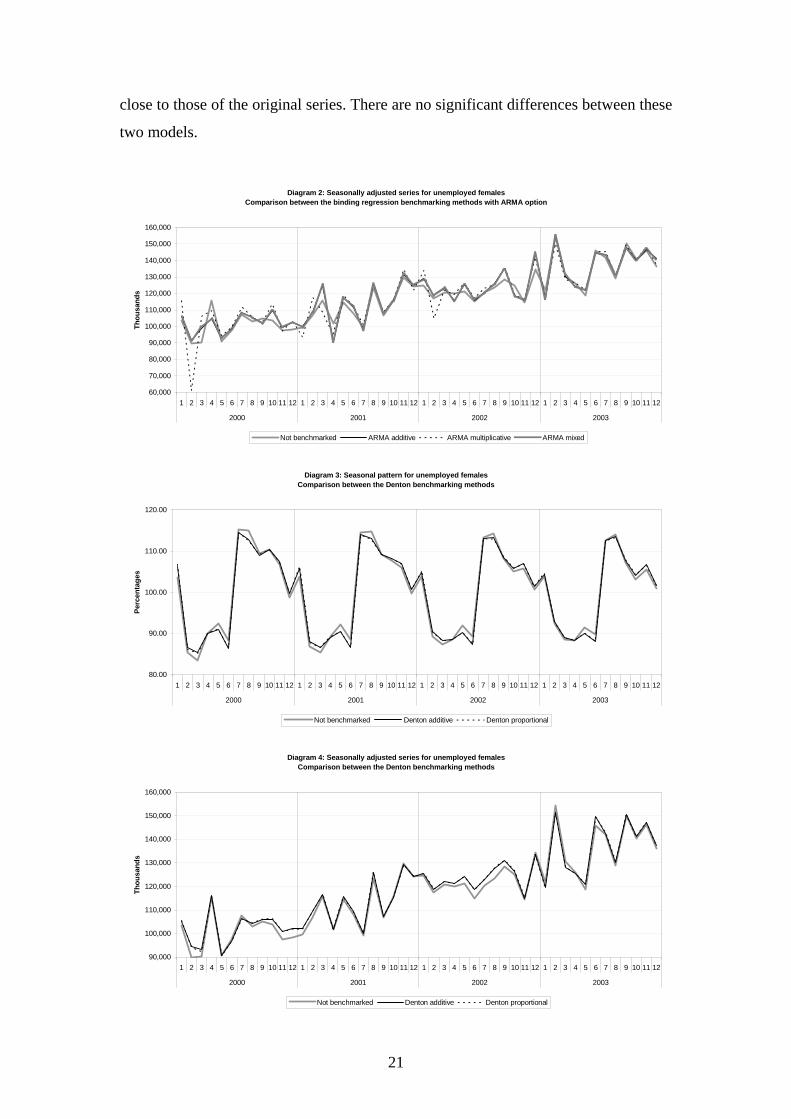
close to those of the original series. There are no significant differences between these

two models.

Diagram 2: Seasonally adjusted series for unemployed femalesComparison between the binding regression benchmarking methods with ARMA option

60,000

70,000

80,000

90,000

100,000

110,000

120,000

130,000

140,000

150,000

160,000

1 2 3 4 5 6 7 8 9 10 11 12 1 2 3 4 5 6 7 8 9 10 11 12 1 2 3 4 5 6 7 8 9 10 11 12 1 2 3 4 5 6 7 8 9 10 11 12

2000 2001 2002 2003

Thou

sand

s


Diagram 3: Seasonal pattern for unemployed femalesComparison between the Denton benchmarking methods

80.00

90.00

100.00

110.00

120.00

1 2 3 4 5 6 7 8 9 10 11 12 1 2 3 4 5 6 7 8 9 10 11 12 1 2 3 4 5 6 7 8 9 10 11 12 1 2 3 4 5 6 7 8 9 10 11 12

2000 2001 2002 2003

Perc

enta

ges

Not benchmarked Denton additive Denton proportional

Diagram 4: Seasonally adjusted series for unemployed femalesComparison between the Denton benchmarking methods

90,000

100,000

110,000

120,000

130,000

140,000

150,000

160,000

1 2 3 4 5 6 7 8 9 10 11 12 1 2 3 4 5 6 7 8 9 10 11 12 1 2 3 4 5 6 7 8 9 10 11 12 1 2 3 4 5 6 7 8 9 10 11 12

2000 2001 2002 2003

Thou

sand

s

Not benchmarked Denton additive Denton proportional

21

5.3.2. Denton models


benchmarked series from the Denton methods, for unemployed females, 2000-2003.


benchmarked data from the Denton methods, for unemployed females, 2000-2003.

In Diagram 3 and Diagram 4 show that the differences between the two Denton

methods are not significant, especially for the seasonally adjusted series. As shown in

Table 4, the proportional Denton method smoothed the unemployed females series

and decreased the relative contribution of the irregular component, in comparison to

all other benchmarking methods.

5.3.3. Unbinding regression models


benchmarked series from the unbinding regression methods, for unemployed females,

2000-2003.


benchmarked data from the unbinding regression methods, for unemployed females,

2000-2003.

All three unbinding regression models provide the best movement preservation and

seasonal adjustment diagnostics in the sense that the differences from the original data

are smaller and the seasonal pattern is unchanged, as displayed in Table 4 and

Diagram 5.

Diagram 5: Seasonal pattern for unemployed females,Comparison between the unbinding benchmarking methods with ARMA options

80.00

90.00

100.00

110.00

120.00

1 2 3 4 5 6 7 8 9 10 11 12 1 2 3 4 5 6 7 8 9 10 11 12 1 2 3 4 5 6 7 8 9 10 11 12 1 2 3 4 5 6 7 8 9 10 11 12

2000 2001 2002 2003

Perc

enta

ges


22

Diagram 6: Seasonally adjusted series for unemployed females, Comparison between the unbinding benchmarking methods with ARMA options

90,000

100,000

110,000

120,000

130,000

140,000

150,000

160,000

1 2 3 4 5 6 7 8 9 10 11 12 1 2 3 4 5 6 7 8 9 10 11 12 1 2 3 4 5 6 7 8 9 10 11 12 1 2 3 4 5 6 7 8 9 10 11 12

2000 2001 2002 2003

Thou

sand

s


Diagram 6 shows that there are no significant differences between the seasonally

adjusted series for unemployed females provided by the three unbinding regression

models, and these series are very close to the not benchmarking seasonally adjusted

data.

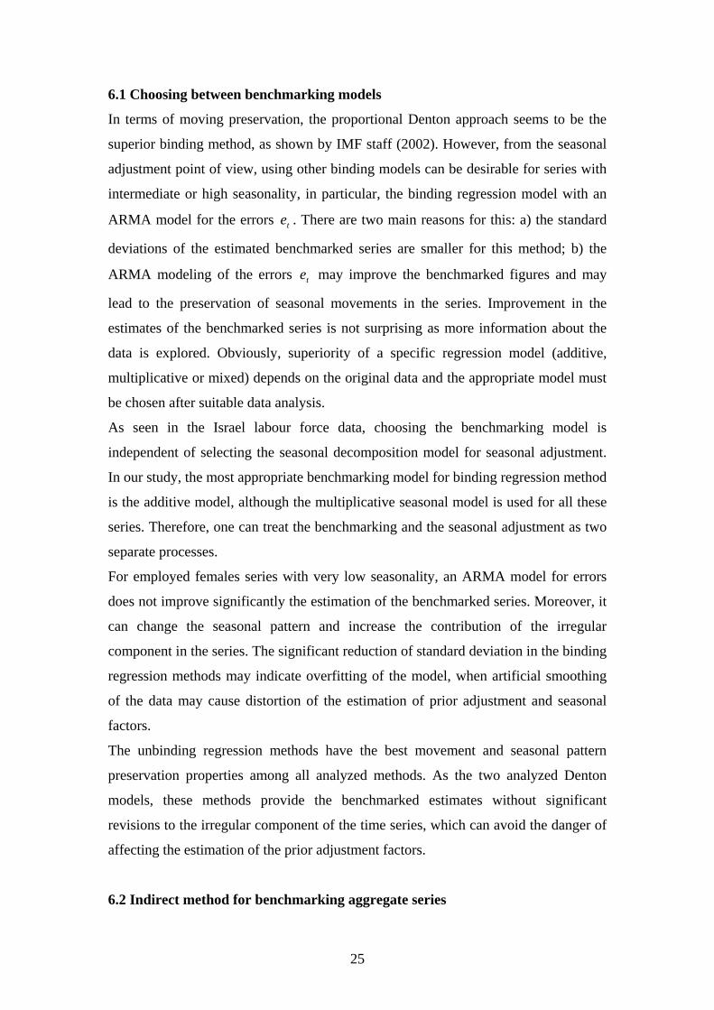
5.3.4. Benchmarking of aggregate series – Total Unemployed Persons

Diagram 7 and Diagram 8 display the total unemployed persons, and its component

series: unemployed males and unemployed females, for 2000-2003. The composite

series is derived from direct and indirect benchmarking techniques. In Diagram 7 all

component series are benchmarked using the Denton proportional method whereas in

Diagram 8 the benchmarking is achieved using the unbinding regression method.

Note that all series are seasonally adjusted by direct and indirect seasonal adjustment

method.

First, let us mention that all benchmarking methods displayed in Diagram 7 and 8

seem to correct the bias in the monthly series. Second, there are no significant

differences between the composite seasonally adjusted series from direct and indirect

seasonal adjustment methods. Also it is shown that the composite seasonally adjusted

series obtained from the Denton proportional benchmarking method and the

unbinding multiplicative regression method are very close to each other. It can be

seen that the seasonally adjusted series is similar in smoothness for the two

benchmarking methods mentioned above, and the amount of revisions in the

seasonally adjusted composite data is small (the movement preservation statistic is

0.5285 for Denton proportional and 0.4359 for unbinding multiplicative regression

23

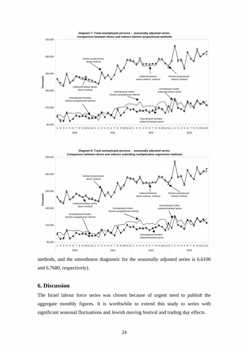
Diagram 7: Total unemployed persons - seasonally adjusted series Comparison between direct and indirect Denton proportional methods

80,000

130,000

180,000

230,000

280,000

330,000

1 2 3 4 5 6 7 8 9 10 11 12 1 2 3 4 5 6 7 8 9 10 11 12 1 2 3 4 5 6 7 8 9 10 11 12 1 2 3 4 5 6 7 8 9 10 11 12

2000 2001 2002 2003

Thou

sand

s

Unbencdir

Denton proportional

oportional method

s es

Unemployed females unbenchmarked series

UnemployDenton propopt

hmarked series ect method

direct method

Unbenchmarked series indirect method

Denton prindirect

Unemployed maleunbenchmarked seriUnemployed males

Denton propoptional methoded females

ional method

Diagram 8: Total unemployed persons - seasonally adjusted series Comparison between direct and indirect unbinding multiplicative regression methods

80,000

130,000

180,000

230,000

280,000

330,000

1 2 3 4 5 6 7 8 9 10 11 12 1 2 3 4 5 6 7 8 9 10 11 12 1 2 3 4 5 6 7 8 9 10 11 12 1 2 3 4 5 6 7 8 9 10 11 12

2000 2001 2002 2003

Thou

sand

s

Unbenchmarked series direct method

Denton proportional direct method

Unbenchmarked series indirect method

Denton proportional indirect method

Unemployed males unbenchmarked seriesUnemployed males

Denton propoptional method

Unemployed females unbenchmarked series

Unemployed females Denton propoptional method

methods, and the smoothness diagnostic for the seasonally adjusted series is 6.6106

and 6.7680, respectively).

6. Discussion The Israel labour force series was chosen because of urgent need to publish the

aggregate monthly figures. It is worthwhile to extend this study to series with

significant seasonal fluctuations and Jewish moving festival and trading day effects.

24

6.1 Choosing between benchmarking models

In terms of moving preservation, the proportional Denton approach seems to be the

superior binding method, as shown by IMF staff (2002). However, from the seasonal

adjustment point of view, using other binding models can be desirable for series with

intermediate or high seasonality, in particular, the binding regression model with an

ARMA model for the errors . There are two main reasons for this: a) the standard

deviations of the estimated benchmarked series are smaller for this method; b) the

ARMA modeling of the errors may improve the benchmarked figures and may

lead to the preservation of seasonal movements in the series. Improvement in the

estimates of the benchmarked series is not surprising as more information about the

data is explored. Obviously, superiority of a specific regression model (additive,

multiplicative or mixed) depends on the original data and the appropriate model must

be chosen after suitable data analysis.

te

te

As seen in the Israel labour force data, choosing the benchmarking model is

independent of selecting the seasonal decomposition model for seasonal adjustment.

In our study, the most appropriate benchmarking model for binding regression method

is the additive model, although the multiplicative seasonal model is used for all these

series. Therefore, one can treat the benchmarking and the seasonal adjustment as two

separate processes.

For employed females series with very low seasonality, an ARMA model for errors

does not improve significantly the estimation of the benchmarked series. Moreover, it

can change the seasonal pattern and increase the contribution of the irregular

component in the series. The significant reduction of standard deviation in the binding

regression methods may indicate overfitting of the model, when artificial smoothing

of the data may cause distortion of the estimation of prior adjustment and seasonal

factors.

The unbinding regression methods have the best movement and seasonal pattern

preservation properties among all analyzed methods. As the two analyzed Denton

models, these methods provide the benchmarked estimates without significant

revisions to the irregular component of the time series, which can avoid the danger of

affecting the estimation of the prior adjustment factors.

6.2 Indirect method for benchmarking aggregate series

25

Diagrams 7 and 8 present the composite series provided by direct and indirect

benchmarking methods and the results are very similar. Naturally , the accounting

links are preserved through the indirect benchmarking, hence this method with good

movement preservation properties may be the preferable one. The advantages of the

indirect benchmarking method exist when the chosen benchmarking model preserves

month-to-month movements and the seasonal pattern in the sub-series. Moreover,

using the indirect benchmarking method matches the concept of indirect seasonal

adjustment, and for the composite series for which indirect seasonal adjustment

method is applied the indirect benchmarking method may be suitable. The motivation

to use the indirect method in benchmarking is the same as in seasonal adjustment; it

allows an easier explanation of the changes in the aggregate data through the changes

in the sub-series. It must be pointed out that the indirect seasonal adjustment approach

is not applied to all composite series. In this case the direct benchmarking methods,

such as Di Fonzo and Marini (2003) technique, or the regression method in section 5

may be more appropriate.

6.3 Quality issues

The quality concepts used in statistical organizations have changed during the last

decades. Nowadays, several statistical agencies have adopted Eurostat quality concept

defined by several criteria Linden (2001) and Haworth and others (2001)). Here we

refer only to the criteria that are relevant for benchmarking.

1. Relevance: a statistical product is relevant if it meets users’ needs.

Benchmarking process meets this criterium because there is a strong demand

by the users (e.g. central banks, economic organizations, universities) for

reliable high-frequency data about socio-economic phenomena that matches

the low-frequency figures. The necessity of seasonally adjusted data forces us

to focus on the benchmarking model with the desired qualities for seasonal

adjustment.

2. Accuracy is defined as the closeness between the estimated value and the

unknown true population value. Applying the benchmarking procedure we

assume that the low-frequency data is more reliable either in terms of standard

deviations, or in terms of closeness to the true figures. This is especially

important for administrative data such as national accounts series.

26

3. Coherence: The coherence between statistics is oriented towards the

comparison of different statistics, which are generally produced in different

ways and for different primary uses. The messages that statistical agencies

convey to users will clearly relate to each other, or at least not contradict each

other. The benchmarking procedure meets this criterium, because by definition

it combines data from two several sources with different frequencies in order

to minimize the existing discrepancies. The indirect benchmarking method

allows adjusting the composite series through the sub-series without violating

accounting constraints in the system of time series. By doing so one can avoid

discrepancies and additional revisions in the original data by applying the

benchmarking procedure n-1 times for the system of n time series.

7. Conclusions

In this paper the properties of the benchmarking procedures are analyzed with a

special emphasis on seasonal adjustment and quality issues. As mentioned in section

7.3, the benchmarking problem meets the statistical quality criteria that were proposed

by the Eurostat and other international statistical organizations: relevance, accuracy

and coherence of the statistical data.

Three benchmarking approaches are considered: the binding regression method with

ARMA model for errors, the Denton method and the unbinding regression method

with ARMA model for errors. The Denton proportional method seems to be the

preferable one among the binding benchmarking methods from the seasonal pattern

preservation point of view. Nevertheless, other benchmarking approaches that

preserve seasonal pattern of the series can be considered. In section 5.3 it was shown

that the binding regression approach may be appropriate for the series with

intermediate and high range of seasonality. For the benchmarking of survey data,

where the survey errors are known, the unbinding regression approach may be useful.

This method provides the best diagnostics for movement and seasonal pattern

preservation.

The benchmarking model for a system of time series, based on the regression

approach, and the indirect benchmarking method for the composite series are

introduced. The direct and the indirect benchmarking methods provide very close

27

composite benchmarked series, for the labour force series. The indirect approach is

preferable especially for series that are seasonally adjusted by indirect method in

order to preserve its advantages. However, for composite series that is seasonally

adjusted by the direct method, the direct benchmarking method using the Denton or

regression approach may be preferable.

28

8. References

1. Chen, Z.G., Cholette, P.A. and Dagum, E.B. (1977), A nonparametric method for benchmarking survey data via signal extraction, Journal of the American Statistical Association, Vol. 92, No. 440, 1563-1571

2. Cholette, P.A., (1979), Adjustment methods of sub-annual series to yearly

benchmarks, Proceeding of the Computer Science 12th Annual Symposium on the Interface, ed. J.F. Gentleman, 358-360

3. Cholette, P.A., (1984), Adjusting sub-annual series to yearly benchmarks,

Survey Methodology, Vol. 10, No. 1, 35-49

4. Cholette, P.A., (1994), Bench program, manual, Working paper TSRA-90-008, Methodology Branch, Statistics Canada.

5. Denton, F.T., (1971), Adjustment of monthly or quarterly series to annual

totals: An approach based on quadratic minimization, Journal of the American Statistical Association, Vol.66, No. 333, 365-377

6. Di Fonzo, T., and Marini, M. (2003), Benchmarking systems of seasonally

adjusted time series according to Denton’s movement preservation principle, Universita di Padova, Working paper 2003.09

7. Durbin, J., and Quenneville, B., (1997), Benchmarking of state-space models,

International Statistical Review, 65, 23-48

8. Fernandez, R.B, (1981), A methodological note on the estimation of time series, Review of Economics and Statistics, 63, 471-476

9. Findley D.F., Monsell, B.C., Bell W.R., Otto, M.C., Chen, B.C., (2000), New

capabilities and methods of the X-12-ARIMA seasonal adjustment program, U.S. Bureau of the Census, USA.

10. Haworth, M., Bergdall, M., Booleman, M., Jones, T., Madaleno, M., (2001),

Quality framework chapter for the European statistical system, Q2001, European Conference on Quality and Methodology in Official Statistics, Stockholm, Sweeden

11. Helfand, S.D., Monsour, N.J., and Trager, M.L., (1977), Historical revision of

current business survey estimates, American Statistical association, Proceedings of the Business and Economic Statistics section, 246-250

12. Hillmer, S.C., and Trabelsi, A., (1987), Benchmarking of economic time

series, Journal of the American Statistical Association, Vol. 82, No. 400, 1064-1071

13. Hillmer, S.C., and Trabelsi, A., (1990), Benchmarking time series with

reliable benchmarks, Applied Statistics, Vol. 39, No. 3, 367-379

29

14. Benchmarking (2002), IMF Textbook, Chapter IV,

www.imf.org/external/pubs/ft/gna/2000/Textbook/ch6.pdf

15. Linden, H., (2001), Data quality - Leadership expert group on quality, Q2001, European Conference on Quality and Methodology in Official Statistics, Stockholm, Sweeden

16. Pfefferman, D., (2002), Small area estimation – new developments and directions, International Statistical review, 70, 125-143

17. Pfefferman, D., and Burck, L., (1990), Robust small area estimation

combining time series and cross-sectional data, Survey Methodology, 16, 217-237

18. Pfefferman, D., and Tiller, R.B., (2003), State-space modeling with correlated measurements with application to small area estimation under benchmarking constraints, Southampton Statistical Sciences Research Institute, Working paper M03/11

30

Documents

Benchmarking of Israeli economic time series and seasonal